2. spectral analysis of discrete signals and systems€¦ · spectral analysis of discrete signals...
TRANSCRIPT

2. Spectral Analysis of Discrete Signals andSystems
in: Signal Processing for Spatial Sound Control
Dr.-Ing. Gerald Enzner
Institut für Kommunikationsakustik (IKA)
Winter Term, 2010/2011
2. Spectral Analysis
2.1 The Fourier Transform (FT)
2.2 The Fourier Transform of Discrete Signals (DSFT)
2.3 Frequency Response of Discrete Systems
2.4 The Discrete Fourier Transform (DFT,FFT)
2.5 Time-Frequency Representation of Audio Signals
Dr.-Ing. Gerald Enzner • Ruhr-Universität Bochum 2/28

2.1 Fourier Transform
The Fourier transform (FT) provides an analysis of signals in terms of itsharmonic components. The FT relates a continuous (time) domain signalxa(t) to its Fourier domain representation Xa(jω)
Xa(jω) =
Z ∞
−∞
xa(t)e−jωtdt
as a function of the angular frequency ω = 2πf . The inverse relationship isgiven by
xa(t) =1
2π
Z ∞
−∞
Xa(jω)ejωtdω .
For signals xa(t) with infinite support, the FT exists if the conditionZ ∞
−∞
|xa(t)|dt < ∞
holds. The inverse FT then reconstructs a signal which is identical to theoriginal signal except for a finite number of discontinuities. Xa(jω) is ingeneral a continuous and non-periodic function of frequency.
Dr.-Ing. Gerald Enzner • Ruhr-Universität Bochum 3/28
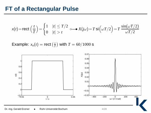
FT of a Rectangular Pulse
x(t)= rect( t
T
)
=
1 |t| ≤ T/2
0 |t| > t−−−−• X(jω)=T si
(
ωT/2)
=Tsin(ωT/2)
ωT/2
Example: xa(t) = rect(
tT
)with T = 60/1000 s
−0.05 0 0.05−0.2
0
0.2
0.4
0.6
0.8
1
t / s
x(t)
−400 −200 0 200 400−0.02
−0.01
0
0.01
0.02
0.03
0.04
0.05
0.06
0.07
ω / (2 π rad)
X(jω
)
Dr.-Ing. Gerald Enzner • Ruhr-Universität Bochum 4/28

Properties of the Fourier Transform
property time domain frequency domain
transform x(t) =1
2π
Z ∞
−∞
X(jω)ejωtdω X(jω) =
Z ∞
−∞
x(t)e−jωtdt
linearity ax1(t) + bx2(t) aX1(jω) + bX2(jω)
conjugation x∗(t) X∗(−jω)
symmetry x(t) is a real valued signal X(−jω) = X∗(jω)
even part xe(t) = 0.5(x(t) + x(−t)) ReX(jω)
odd part xo(t) = 0.5(x(t) − x(−t)) jImX(jω)
convolution x1(t) ∗ x2(t) X1(jω) · X2(jω)
time shift x(t − t0) e−jωt0 X(jω)
modulation x(t)ejωM t X(j(ω − ωM))
scaling x(at), a ∈ R, a 6= 01|a|
X“
jω
a
”
Parseval’s theorem
Z ∞
−∞
|x(t)|2dt =1
2π
Z ∞
−∞
|X(jω)|2dω
Dr.-Ing. Gerald Enzner • Ruhr-Universität Bochum 5/28
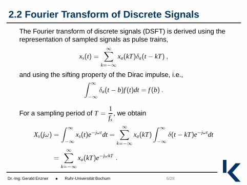
2.2 Fourier Transform of Discrete Signals
The Fourier transform of discrete signals (DSFT) is derived using therepresentation of sampled signals as pulse trains,
xs(t) =
∞∑
k=−∞
xa(kT)δa(t − kT) ,
and using the sifting property of the Dirac impulse, i.e.,∫
∞
−∞
δa(t − b)f (t)dt = f (b) .
For a sampling period of T =1fs
, we obtain
Xs(jω) =
∫∞
−∞
xs(t)e−jωtdt =
∞∑
k=−∞
xa(kT)
∫∞
−∞
δ(t − kT)e−jωtdt
=
∞∑
k=−∞
xa(kT)e−jωkT .
Dr.-Ing. Gerald Enzner • Ruhr-Universität Bochum 6/28

Fourier Transform of Discrete Signals
Xs(jω) is a continuous and periodic function of the angular frequencyω and hence also of frequency f . To see this we note that thecomplex phasor
e−jωkT = e−j2πfkT = cos(2πfkT) − j sin(2πfkT)
is periodic in ω with period ω =2π
T= 2πfs. Therefore,
Xs(j(ω +2πℓ
T)) = Xs(jω) for any ℓ ∈ Z .
In digital signal processing, we treat a sampled signal xs(t) on anabstract level as a sequence of numbers x(k). This allows a generaltreatment of signal processing methods without reference to thephysical aspects (time or frequency scale) of the signal. Occasionally,we remind ourselves that the sequence x(k) was obtained bysampling a continuous-time signal xa(t) with sampling rate fs.
Dr.-Ing. Gerald Enzner • Ruhr-Universität Bochum 7/28

Fourier Transform of Discrete Signals
To facilitate the treatment of sampled signals in the Fourier domain,we normalize the frequency variable f on the sampling rate fs andintroduce the normalized angular frequency Ω = ωT = 2πfT = 2π f
fs.
We then obtain the Fourier Transform of Discrete Signals (DSFT) andits inverse relationship
X(ejΩ) =
∞∑
k=−∞
x(k)e−jΩk x(k) =1
2π
∫ π
−π
X(ejΩ)ejΩkdΩ .
Note, that the inverse transform is evaluated over one period of thespectrum only. X(ejΩ) is a complex quantity:
X(ejΩ) = ReX(ejΩ) + jImX(ejΩ) = |X(ejΩ)|ejφ(Ω)
where |X(ejΩ)| is the amplitude spectrum and φ(Ω) ∈ −π, π is thephase. Frequently, we consider the logarithm of the amplitudespectrum 20 log10(|X(ejΩ)|) = |X(ejΩ)|/dB.
Dr.-Ing. Gerald Enzner • Ruhr-Universität Bochum 8/28

Comparison: FT and DSFT of a Rectangular Pulse
−0.05 0 0.05−0.2
0
0.2
0.4
0.6
0.8
1
t / s
x(t)
−400 −200 0 200 400−0.02
−0.01
0
0.01
0.02
0.03
0.04
0.05
0.06
0.07
ω / (2 π rad)
X(jω
)
−10 −5 0 5 10−0.2
0
0.2
0.4
0.6
0.8
1
k
x(k)
−2 −1 0 1 2−4
−2
0
2
4
6
8
10
12
14
Ω / (2 π)
X(e
jΩ)
∑(N−1)/2ℓ=−(N−1)/2 δ (k − ℓ) −−−−• sin(ΩN/2)
sin(Ω/2)
Dr.-Ing. Gerald Enzner • Ruhr-Universität Bochum 9/28
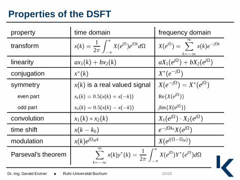
Properties of the DSFT
property time domain frequency domain
transform x(k) =1
2π
Z
π
−π
X(ejΩ)ejΩkdΩ X(ejΩ) =∞
X
k=−∞
x(k)e−jΩk
linearity ax1(k) + bx2(k) aX1(ejΩ) + bX2(ejΩ)
conjugation x∗(k) X∗(e−jΩ)
symmetry x(k) is a real valued signal X(e−jΩ) = X∗(ejΩ)
even part xe(k) = 0.5(x(k) + x(−k)) ReX(ejΩ)
odd part xo(k) = 0.5(x(k) − x(−k)) jImX(ejΩ)
convolution x1(k) ∗ x2(k) X1(ejΩ) · X2(ejΩ)
time shift x(k − k0) e−jΩk0X(ejΩ)
modulation x(k)ejΩM k X(ej(Ω−ΩM))
Parseval’s theorem∞
X
k=−∞
x(k)y∗(k) =1
2π
Z
π
−π
X(ejΩ)Y∗(ejΩ)dΩ
Dr.-Ing. Gerald Enzner • Ruhr-Universität Bochum 10/28

Example: DSFTof Exponential x(k) = aku(k), a = 0.7
−1.5 −1 −0.5 0 0.5 10
0.5
1
1.5
2
2.5
3
3.5
4
Ω / (2 π rad)
Re
X(e
jΩ)
−1.5 −1 −0.5 0 0.5 1−2
−1.5
−1
−0.5
0
0.5
1
1.5
2
Ω / (2 π rad)
ImX
(ejΩ
)
−1.5 −1 −0.5 0 0.5 10
0.5
1
1.5
2
2.5
3
3.5
4
Ω / (2 π rad)
|X(e
jΩ)|
−1.5 −1 −0.5 0 0.5 1−2
−1.5
−1
−0.5
0
0.5
1
1.5
2
Ω / (2 π rad)
φ(Ω
)
Dr.-Ing. Gerald Enzner • Ruhr-Universität Bochum 11/28
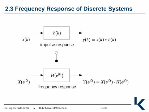
2.3 Frequency Response of Discrete Systems
impulse response
frequency response
x(k) y(k) = x(k) ∗ h(k)
h(k)
X(ejΩ) Y(ejΩ) = X(ejΩ) · H(ejΩ)
H(ejΩ)
Dr.-Ing. Gerald Enzner • Ruhr-Universität Bochum 12/28

Example: Delay System
h(k) = δ(k − k0) −−−−• H(ejΩ) =∞∑
k=−∞δ(k − k0)e−jΩk = e−jΩk0
0 0.2 0.4 0.6 0.8 1−2000
−1500
−1000
−500
0
Normalized Frequency (×π rad/sample)
Pha
se (
degr
ees)
0 0.2 0.4 0.6 0.8 1−1
−0.5
0
0.5
1
Normalized Frequency (×π rad/sample)
Mag
nitu
de (
dB)
k0 = 10
Dr.-Ing. Gerald Enzner • Ruhr-Universität Bochum 13/28
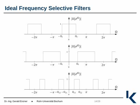
Ideal Frequency Selective Filters
0
0
1
1
0
1
Ω
Ω
Ω
π
π
π
2π
2π
2π
−π
−π
−π
−2π
−2π
−2π
|X(ejΩ)|
|X(ejΩ)|
|X(ejΩ)|
Ωc
Ωc
Ωc1 Ωc2
−Ωc
−Ωc
−Ωc1−Ωc2
Dr.-Ing. Gerald Enzner • Ruhr-Universität Bochum 14/28
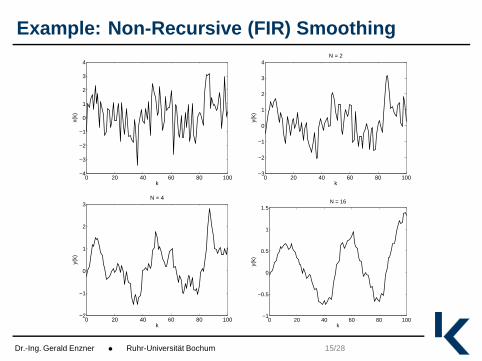
Example: Non-Recursive (FIR) Smoothing
0 20 40 60 80 100−4
−3
−2
−1
0
1
2
3
4
k
x(k)
0 20 40 60 80 100−3
−2
−1
0
1
2
3
4
k
y(k)
N = 2
0 20 40 60 80 100−2
−1
0
1
2
3
k
N = 4
y(k)
0 20 40 60 80 100−1
−0.5
0
0.5
1
1.5
k
y(k)
N = 16
Dr.-Ing. Gerald Enzner • Ruhr-Universität Bochum 15/28
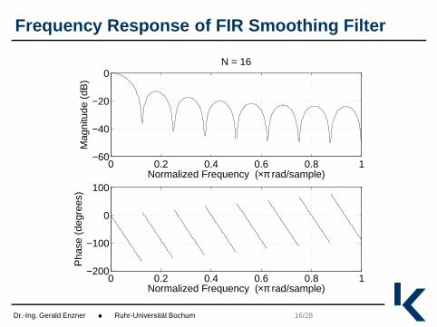
Frequency Response of FIR Smoothing Filter
0 0.2 0.4 0.6 0.8 1−200
−100
0
100
Normalized Frequency (×π rad/sample)
Pha
se (
degr
ees)
0 0.2 0.4 0.6 0.8 1−60
−40
−20
0
Normalized Frequency (×π rad/sample)
Mag
nitu
de (
dB)
N = 16
Dr.-Ing. Gerald Enzner • Ruhr-Universität Bochum 16/28
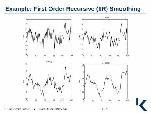
Example: First Order Recursive (IIR) Smoothing
0 20 40 60 80 100−4
−3
−2
−1
0
1
2
3
4
k
x(k)
0 20 40 60 80 100−3
−2
−1
0
1
2
3
4
k
y(k)
α = 0.333
0 20 40 60 80 100−2
−1
0
1
2
3
k
y(k)
α = 0.6
0 20 40 60 80 100−1
−0.5
0
0.5
1
1.5
k
y(k)
α = 0.8824
Dr.-Ing. Gerald Enzner • Ruhr-Universität Bochum 17/28

Frequency Response of IIR Smoothing Filter
0 0.2 0.4 0.6 0.8 1−80
−60
−40
−20
0
Normalized Frequency (×π rad/sample)
Pha
se (
degr
ees)
0 0.2 0.4 0.6 0.8 1−30
−20
−10
0
Normalized Frequency (×π rad/sample)
Mag
nitu
de (
dB)
α = 0.8824
Dr.-Ing. Gerald Enzner • Ruhr-Universität Bochum 18/28

2.4 Definition of the DFT
The Discrete Fourier Transform (DFT) is given by
Xµ =
M−1∑
k=0
x(k)e−j 2πµkM , µ = 0, . . . , M − 1
and the inverse relationship by
x(k) =1M
M−1∑
µ=0
Xµej 2πµkM , µ = 0, . . . , M − 1 .
The coefficients of the DFT are spaced by ∆Ω = 2πM on the
normalized frequency axis Ω. Therefore, we may think of the DFT asan approximation of a continuous spectrum at discrete frequenciesΩµ = 2πµ
M . When the signal samples x(k) are generated by means ofsampling a continuous signal x(t) with sampling period T = 1
fs, the
coefficients of the DFT are spaced as fµ = µfsM , therefore ∆f = fs
M .
Dr.-Ing. Gerald Enzner • Ruhr-Universität Bochum 19/28
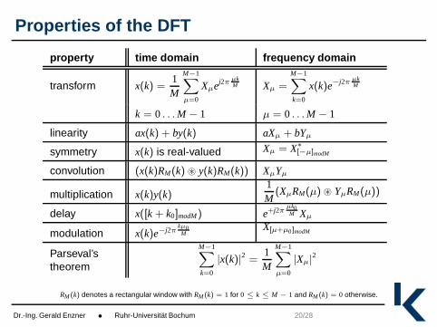
Properties of the DFT
property time domain frequency domain
transform x(k) =1M
M−1X
µ=0
Xµej2πµkM Xµ =
M−1X
k=0
x(k)e−j2πµkM
k = 0 . . . M − 1 µ = 0 . . . M − 1
linearity ax(k) + by(k) aXµ + bYµ
symmetry x(k) is real-valued Xµ = X∗[−µ]modM
convolution (x(k)RM(k) ⊛ y(k)RM(k)) XµYµ
multiplication x(k)y(k)1M
(XµRM(µ) ⊛ YµRM(µ))
delay x([k + k0]modM) e+j2πµk0
M Xµ
modulation x(k)e−j2πkµ0
MX[µ+µ0 ]modM
Parseval’stheorem
M−1X
k=0
|x(k)|2 =1M
M−1X
µ=0
|Xµ|2
RM (k) denotes a rectangular window with RM (k) = 1 for 0 ≤ k ≤ M − 1 and RM (k) = 0 otherwise.
Dr.-Ing. Gerald Enzner • Ruhr-Universität Bochum 20/28

2.5 Zeit-Frequenz Darstellung von Audiosignalen
0 1 2 3 4 5 6 7 8 9−1
−0.5
0
0.5
1
Am
pliu
tude
0 1 2 3 4 5 6 7 8 9−1
−0.5
0
0.5
1
Zeit [Sekunden]
Am
pliu
tude
Sprache
Musik
Dr.-Ing. Gerald Enzner • Ruhr-Universität Bochum 21/28
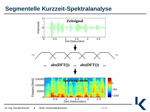
Segmentelle Kurzzeit-Spektralanalyse
......abs(DFT()) abs(DFT())...
... ...
Zeit [Sekunden]
Freq
uenz
[Her
tz]
0.5 1 1.5 2 2.50
5000
10000
15000
−100
−50
0
0 0.5 1 1.5 2 2.5−1
0
1
Zeit [Sekunden]A
mpl
iutu
de
Spectrogramm
Zeitsignal
Dr.-Ing. Gerald Enzner • Ruhr-Universität Bochum 22/28

Audio SpektrogrammeF
requ
enz
[Her
tz]
1 2 3 4 5 6 7 8 90
5000
10000
15000
Zeit [Sekunden]
Fre
quen
z [H
ertz
]
1 2 3 4 5 6 7 8 90
5000
10000
15000
−100
−50
0
−100
−50
0
Sprache
Musik
Dr.-Ing. Gerald Enzner • Ruhr-Universität Bochum 23/28
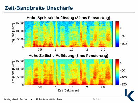
Zeit-Bandbreite UnschärfeF
requ
enz
[Her
tz]
0.5 1 1.5 2 2.50
5000
10000
15000
Zeit [Sekunden]
Fre
quen
z [H
ertz
]
0.5 1 1.5 2 2.50
5000
10000
15000
−100
−50
0
−150
−100
−50
0
Hohe Spektrale Auflösung (32 ms Fensterung)
Hohe Zeitliche Auflösung (8 ms Fensterung)
Dr.-Ing. Gerald Enzner • Ruhr-Universität Bochum 24/28
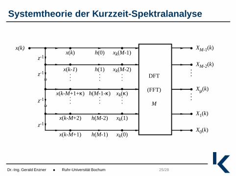
Systemtheorie der Kurzzeit-Spektralanalyse
x(k)
DFT
(FFT)
M
XM-1(k)
XM-2(k)
Xµ(k)
X1(k)
X0(k)
z-1
z-1
z-1
z-1
...
...
xk(M-2)
xk(M-1)
xk(κ)
xk(1)
xk(0)
...
...
h(0)
h(1)
h(M-1-κ)
h(M-2)
h(M-1)
...
...
x(k-M+1+κ)
x(k)
x(k-1)
x(k-M+2)
x(k-M+1)
...
...
Dr.-Ing. Gerald Enzner • Ruhr-Universität Bochum 25/28
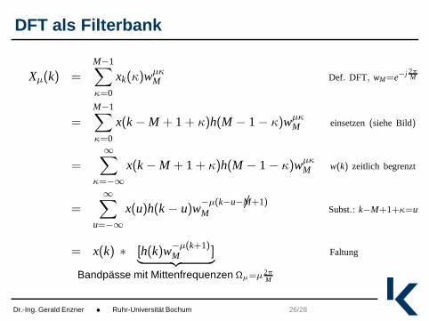
DFT als Filterbank
Xµ(k) =M−1∑
κ=0
xk(κ)wµκM Def. DFT, wM=e−j 2π
M
=
M−1∑
κ=0
x(k − M + 1 + κ)h(M − 1 − κ)wµκM einsetzen (siehe Bild)
=
∞∑
κ=−∞
x(k − M + 1 + κ)h(M − 1 − κ)wµκM w(k) zeitlich begrenzt
=∞∑
u=−∞
x(u)h(k − u)w−µ(k−u−M+1)/M Subst.: k−M+1+κ=u
= x(k) ∗ [h(k)w−µ(k+1)M ]
︸ ︷︷ ︸
Bandpässe mit Mittenfrequenzen Ωµ=µ 2π
M
Faltung
Dr.-Ing. Gerald Enzner • Ruhr-Universität Bochum 26/28
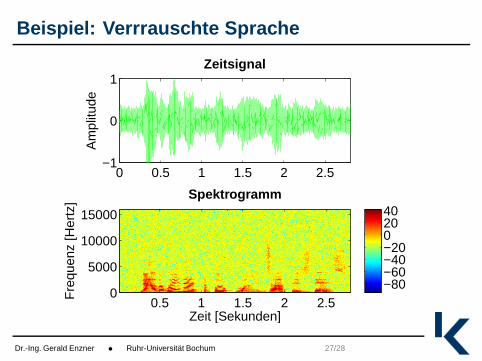
Beispiel: Verrrauschte Sprache
0 0.5 1 1.5 2 2.5−1
0
1A
mpl
itude
Zeit [Sekunden]
Fre
quen
z [H
ertz
]
0.5 1 1.5 2 2.50
5000
10000
15000
−80−60−40−2002040
Zeitsignal
Spektrogramm
Dr.-Ing. Gerald Enzner • Ruhr-Universität Bochum 27/28

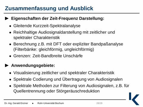
Zusammenfassung und Ausblick
Eigenschaften der Zeit-Frequenz Darstellung:
• Gleitende Kurzzeit-Spektralanalyse
• Reichhaltige Audiosignaldarstellung mit zeitlicher undspektraler Charakteristik
• Berechnung z.B. mit DFT oder expliziter Bandpaßanalyse(Filterbänke: gleichförmig, ungleichförmig)
• Grenzen: Zeit-Bandbreite Unschärfe
Dr.-Ing. Gerald Enzner • Ruhr-Universität Bochum 28/28
Zusammenfassung und Ausblick
Eigenschaften der Zeit-Frequenz Darstellung:
• Gleitende Kurzzeit-Spektralanalyse
• Reichhaltige Audiosignaldarstellung mit zeitlicher undspektraler Charakteristik
• Berechnung z.B. mit DFT oder expliziter Bandpaßanalyse(Filterbänke: gleichförmig, ungleichförmig)
• Grenzen: Zeit-Bandbreite Unschärfe
Anwendungsgebiete:
• Visualisierung zeitlicher und spektraler Charakteristik
• Spektrale Codierung und Übertragung von Audiosignalen
• Spektrale Methoden zur Filterung von Audiosignalen, z.B. fürQuellentrennung oder Störgeräuschreduktion
Dr.-Ing. Gerald Enzner • Ruhr-Universität Bochum 28/28