introduction - princeton universityrcarmona/download/fe/cw1.pdfmoreover, since liquidity providers...

HIGH FREQUENCY MARKET MAKING

RENE CARMONA AND KEVIN WEBSTER

Abstract. Since they were authorized by the U.S. Security and Exchange Commission in 1998,electronic exchanges have boomed, and by 2010 high frequency trading accounted for over 70% of

equity trades in the US. Such markets are thought to increase liquidity because of the presence

of market makers, who are willing to trade as counterparties at any time, in exchange for a fee,the bid-ask spread. In this paper, we propose an equilibrium model showing how such market

makers provide liquidity. The model relies on a codebook for client trades, the implied alpha.After solving the individual clients optimization problems and identifying their implied alphas, we

frame the market maker stochastic optimization problem as a stochastic control problem with an

infinite dimensional control variable. Assuming either identical time horizons for all the clients,or a stochastic partial differential equation model for their beliefs, we solve the market maker

problem and derive tractable formulas for the optimal strategy and the resulting limit-order book

dynamics.

1. Introduction

Electronic exchanges play an increasingly important role in financial markets and market mi-crostructure became the key to understanding them. Here market microstructure is understoodas the study of the trading mechanisms used for financial securities [11]. High frequency tradingstrategies depend very strongly on these mechanisms which in turn, vary from market to market.Three main themes were proposed to unite the common features of most of these markets [11].

(1) The first theme is the limit-order book, where agents can post trading intentions at pricesabove (ask) or below (bid) the mid-price, which is regarded as the current fair price for thesecurity. These posts, called limit-orders, can then lead to executions if they are paired witha matching order. In this case, the initial agent, commonly known as the liquidity provider,gains a small amount of money, having sold at the ask or bought at the bid. It is said inthat case that the liquidity taker has paid a liquidity fee for the right to trade immediately.

(2) The second theme is adverse selection due to asymmetric sources of information. It is basedon the principle that liquidity takers choose which limit-orders are actually executed, andwhen. Moreover, since liquidity providers publicly announce their intentions by postingtheir limit-orders, and these two market rules create an information bias in favor of liquiditytakers that compensates for the liquidity fee.

(3) The last theme is statistical predictions. All agents on electronic markets attempt to predictprices on a short time scale. Such predictions are possible both because of the existenceof private information and the actual market mechanisms that create short-range price cor-relations. While statistical predictions are used by all traders on electronic markets, theobjectives of these agents vary widely. Some make their profits from these predictions, whileothers just reduce their transaction costs by trading smartly.

Date: October 12, 2012.Key words and phrases. Limit-order book, Transaction costs, Stochastic partial differential equations, Pontryagin

maximum principle, Market making.

1

2 RENE CARMONA AND KEVIN WEBSTER

After the liquidity crisis of 2008, liquidity became the central object of interest for market mi-crostructure. Liquidity is rarely defined precisely, although intuitively, it should quantify how diffi-cult it is to engage in a trade. Commonly accepted measures of liquidity are the bid-ask spread1 andthe volume present in a limit-order book. We tie these two quantities together by modeling what wewill call the liquidity cost curve, or simply cost curve. We define this to be the total fee paid by theliquidity taker as a function of the volume asked for. If the liquidity taker only executes limit-ordersat the best ask or bid, the fee will be equal to the bid-ask spread times the volume. Some clients,however, might wish to go beyond the best bid or ask and take more volume from the market. Themarginal fee then becomes a function of the volume.

Trade volumes are difficult to model, in part because they are so dependent on liquidity takers’decisions and their execution strategies. Empirically, trade volumes present very heavy tails and arestrongly autocorrelated ([6]): there are frequent outliers, buys tend to follow buys, and sells tendto follow sells, which is what makes them hard to evaluate statistically. Limit-orders, on the otherhand, are mean-reverting and have been widely studied in the literature (see, for instance, [6, 7, 19]).The interplay between trend-following liquidity takers and mean-reverting liquidity providers is whatmakes the market reach the critical state of diffusion, as seen in [5]. From a modeling stand point, allthese attributes are what makes a direct statistical description of trade volumes so difficult, whichis why the introduction of a codebook is desirable.

1.1. Market making. Market makers are a special class of liquidity providers. They essentiallyact as a scaled down version of the market itself, always providing limit-orders on both sides of themid-price. How these limit-orders are placed in terms of volume, distribution, and distance from themid-price, determines the pricing strategy. We can therefore define the liquidity curve associatedwith a market maker’s pricing strategy. The agents trading with a market maker are considered ashis clients. Market making is a purely passive strategy that essentially corresponds to the service ofproviding liquidity to the market against a fee. This strategy makes money as long as the pricingaccurately anticipates future price variations. The first step towards that objective is to find a modelfor client volumes that is consistent with price dynamics.

There are two schools of thoughts on market making models. The first focuses on inventory risk.There, the market maker has a preferred inventory position and prices according to his risk aversionto diverging inventory levels. Some of the first models of this type are [10, 4], which can be foundin [11]. The second, initiated by [14], focuses on adverse selection, usually distinguishing betweeninformed and noise trades. This paper belongs to the second line of thought.

According to our stylized definition of a market maker, the latter does not possess a view on themarket. Clients, on the other hand, have views on the market and this leads to trading needs. Whenthis view is short term, then the client has a statistical edge on the rest of the market and tries topush that edge to make a short term profit. But even when the view is long term, the client willstill attempt to minimize transaction costs by predicting prices on a short time scale. Long-termstrategies and liquidity constraints can therefore be modeled as noise around optimal short termexecution strategies. The intuition behind this is that long term constraints, while the main motivesbehind most trades, will not necessarily dictate their execution. This is the case because there areincreasingly more layers between the entity that formulates the long term strategy (for exampleinvestment banks or hedge funds) and the one that actually executes it (for example brokers orexecution engines). But only the latter actually has a short term view on the market, which is what

1The bid-ask spread is defined as the price difference between the lowest ask and the highest bid in the limit-orderbook.

HIGH FREQUENCY MARKET MAKING 3

the market maker is interested in. Optimal executions based on short term beliefs and associatedtrade volumes form therefore the cornerstone of the upcoming analysis and will link prices to trades.

1.2. Alpha. Alpha is the term often used to signify that a client has a directional view on themarket. In an adverse selection model the aim of any market maker is to discover this view andhedge against it. Most papers (see for example [2, 5, 18, 11]) introduce a notion of market impactor response function, to study the relationship between trades and prices. Trade size is often –though not always – included, and a lot of work has been done to fit various curves to the responsefunction. A large number of papers on execution strategies ([1, 2, 3, 16]) rely heavily on this notionof market impact. So do most practitioners. Essentially, alpha and market impact are the samequantity, even though the stories told to justify these concepts are quite different. In the marketimpact literature, the premise is that a trade causes a price movement, while alpha is viewed as anattempt at predicting the movement. Response function is a more neutral term that allows for bothinterpretations.

In this paper, we present a simple model for client decisions that proves, under very generalassumptions, a systematic relationship between trade sizes and short term expected price variations.It states that marginal costs should equal expected price variations. This is an intuitive result giventhat price variations are the marginal gains of a risk-neutral client. In this model, each client has ashort term view on the market and trades optimally according to this view: his optimal executionstrategy depends upon his belief. The theoretical notion of implied alpha appears quite naturallyfrom the stochastic optimal control problem that defines the client’s model.

On the market maker side, our model tries to capture the fact that market makers do not act ona personal view of the market. The market maker uses the notion of client implied alpha to infer anapproximate price process from his clients’ behaviors, essentially aggregating the views of his clientsto form a probability distribution on the price. The optimal order book strategy then replicates thisdistribution, with a corrective term that takes into account the profitability of trades, that is, thetrade-off between spread and volume.

1.3. Results. The thrust of this paper is to propose a framework in which a market making strategyappears endogenously. This framework is based on

(1) a result to imply a market view from client trades under a simple yet robust model of clientbehavior;

(2) a procedure for the market maker to infer his own view on the market from that of hisclients;

(3) a profitability function that measures how profitable a posted volume on the order book islikely to be;

(4) a penalizing term taking into account possible feedback effects of the market maker’s decision.

The last part will be motivated by the idea that, just as the market maker implies information fromhis clients’ trades, clients can infer information from his order book. Our hypotheses are chosen, andour results are derived, in order to make the market making problem tractable. Once the theoreticalframework is put in place, the market maker optimal control problem is formulated and solved,leading to an explicit market making strategy.

The story told by the model is closest to that of the informed trade literature [14], althoughone major difference is that there is no clear cut distinction between informed and noise traders.Our conservative market maker assumes that all of his clients’ implied alphas carry information.Moreover, the existence of at least one informed trader underpins the estimation formula used bythe market maker. The paper also relates strongly to both the market impact [2, 5, 18, 11] andoptimal execution [1, 3, 2, 16] literatures. A cost function ct and an order book γ′′t are derived


endogenously from the premises of the model. We hope that the proposed implied alpha codebookwill find applications in other limit-order book models. Finally, while we ignore inventory risk tomake our market maker risk-neutral, our approach still relates to utility function and inventorymodels such as [4, 10].

The results of the paper are organized in four sections. First, the setup for the model is given,which includes a methodology for modeling heterogeneous beliefs and transaction costs. Second, asimple client model is presented and solved, leading to a relationship between trades and alphas whichmotivates the market maker’s choice for a codebook. Third, the market maker model is built step bystep, starting from the client model and working through a series of results and approximations tolead to a reasonable control problem. Last, the market maker’s problem is solved and the dynamicsof the order book are determined analytically, For the sake of definiteness, we focus on a tractableexample for which we compute the two-humped limit order book shape. An appendix is added atthe end of the paper to provide the proofs of two technical results which, had they been included inthe text, could have distracted from the main objective of the modeling challenge.

2. Setup of the model

In this section, all the elements of the model are presented.

2.1. Heterogeneous beliefs on the price. Consider n clients and one market maker who interacton an electronic exchange, with n very large. We will denote by i ∈ 1...n a client index, andk ∈ 0...n a generic index, with k = 0 corresponding to the market maker. We first introduce thefollowing setting for the model:

(1) a filtered probability space (Ω,F , (Ft)t≥0 ,P) representing the “real life” filtration and prob-ability measure. The filtration is generated by a d-dimensional P Wiener process Wt.

(2) a different filtration and measure ((Fkt )t≥0,Pk) for each of the agents. Assume furthermorethat Fkt ⊂ Ft, that Pk|Fkt and P|Fkt are equivalent and that P0|F0

t= P|F0

t.

(3) a dk-dimensional P Wiener process W kt that generates the filtration (Fkt )t≥0.

(4) a price process pt which is an Ito process adapted to all the filtrations((Fkt)t≥0

)k=0...n

.

(5) the drift and volatility of pt grow at most polynomially in t under all probability measures.

where the last hypothesis must be understood in the a.s. and L2 sense.Let

dpt = atdt+ σtdWt (2.1)

be the Ito decomposition of pt under(

(Ft)t≥0 ,P)

. Hypotheses 2 and 3 imply that there exists an(Fkt)t≥0

adapted process rkt such that

W kt = Bkt +

∫ t

0

rksds (2.2)

for some Pk|Fkt Wiener process Bkt and with r0t = 0. Because W k is dk dimensional, so are rkt and

Bkt . Furthermore, by the martingale representation theorem, given that W kt is a P martingale, there

exists an (Ft)t≥0 adapted, dk × d dimensional matrix Σkt such that

dW kt = Σkt dWt (2.3)

Finally, agent k has the following view on the market under((Fkt)t≥0

,Pk)

:

dpt = akt dt+ σkt dBkt (2.4)


with σt = σkt Σkt and akt = at + σkt rkt . In particular, σt needs to live in the intersection of the images

of all the(Σkt)T

for pt to be adapted to all the filtrations. Note that the dk is allowed to differ from

one agent to another, in which case the σkt must be of different dimensions and hence differ.In conclusion, all the agents have views on the price process that potentially conflict with each

other’s probability measure and even filtration, but can be compared coherently within the largerprobability space (Ω,F , (Ft)t≥0 ,P).

Example 2.1. Consider the case where you have three Wiener processes W 1, W 2 and W 3. Let

pt = W 1t +W 2

t +W 3t , F it = σ

((W is

)s≤t , (ps)s≤t

)and rit = f(W i

t ). You then have that:

dpt = dW 1t + dW 2

t + dW 3t under P

= f(W 1t )dt+ dB1,1

t + dB1,2t under P1

= f(W 2t )dt+ dB2,1

t + dB2,2t under P2

where the two last decompositions are not adapted with respect to the other filtration, but the priceprocess is nevertheless adapted to both filtrations.

2.2. Transaction costs. We now allow trades among agents. All clients have a cumulative positionLi in the asset, which starts off at 0 at the beginning of the trading period. For the market maker,we rescale all the quantities according to the number of clients, hence L0

t is his average cumulativeposition per client. Clients control their position through its first derivative, lit but incur transactioncosts. The market maker, on the other hand, has no direct control over his position, but receives theliquidity fee ct. To be precise, the market maker announces to his clients a cost function l 7−→ ct(l),which denotes the price of trading at speed l at moment t. A client then chooses her preferredtrading volume lit, and pays ct(l

it) in total transaction fees. We make the following hypotheses on

these two processes:

(1) The trade volume process lit for each client is adapted to(F it)t≥0

and(F0t

)t≥0

.

(2) The cost function process ct is adapted to all filtrations.(3) Marginal costs are defined: c′t is almost everywhere continuous.(4) Clients may choose not to trade, ct(0) = 0 and the mid-price is well defined at pt, c

′t(0) = 0.

(5) Marginal costs increase with volume: ct is convex.(6) There is a fixed amount of liquidity the market maker offers.

Hypotheses 1 and 2 describe the information the different agents have access to. 3-5 are intuitiveproperties that the cost function must verify to make sense in terms of transaction costs. Finally,the hypothesis 6 is left purposefully vague, because it is best expressed with notation we introducenow.

2.2.1. Duality and link to the order book. This section introduces a change of variable that is bothmathematically convenient and will carry deeper financial meaning when the model is solved. Thenew variable γ is defined as follows:

γt(α) = supl∈supp(ct)

(αl − ct(l)) (2.5)

Under the assumptions ct ∈ C1, convex and ct(0) = 0, this is equivalent to defining γ′t = (c′t)−1 and

γt(0) = 0. In that case, γt is simply the Legendre transform of ct. The following properties can bederived:


(1) The Legendre transform maps the space of convex functions onto itself. It is its own in-verse. In particular, γ′′t , where the second derivative has to be understood in the sense ofdistributions, is a positive, finite measure.

(2) ∀α ∈ R,∀l ∈ R, γt(α) + ct(l) ≥ αl (Fenchel’s inequality), with equality for α∗ = c′t(l) orl∗ = γ′t(α).

(3) γ′′t is a description of the limit-order book of the market maker. Indeed, it representsmarginal volumes as a function of marginal costs. The property γ′′t being a positive, finitemeasure corresponds to the fact that the market maker can only post positive, finite volumeson the order book.

This means we can actually replace ct by the second derivative of its dual γ′′t as the control variableof the market maker. Similarly, αit is the dual to the client’s control variable lit. Call γ′′t the marketmaker’s liquidity offer and αit the client’s implied alpha. The second terminology will be explainedlater. We therefore recast all the hypotheses with these new dual variables:

(1) The implied alpha process αit for each client is adapted only to(F it)t≥0

and(F0t

)t≥0

.

(2) The liquidity process γ′′t for each market maker is adapted to all filtrations.(3) We have lit = γ′t

(αit)

and αit = c′t(lit).

(4) Clients may choose not to trade and the order book is centered around the mid-price:γt(0) = 0 and γ′t(0) = 0.

(5) Only positive, finite volumes are posted on a market maker’s liquidity offer: γ′′t is a positive,finite measure.

(6) The total mass of γ′′t is fixed. For convenience sake we will renormalize it to one, making γ′′ta probability measure.

As a consequence of 3-5, lit is bounded. Furthermore, γ′′t therefore lives on the space of finitemeasures, which is a complete, separable metric space under the Levy-Prokhorov metric and aconvex set.

2.3. Putting it all together. We summarize the model. First a public price process pt is given.Assume it is exogenously given to every one, that is, all the agents consider that they have noimpact on the price under their probability measure, and only try to estimate its future movements.Then, a public liquidity offer, which can both be followed either by the cost function ct or its dual,γ′′t is announced. Clients pick their trade volumes lit, or equivalently, their implied alphas αit. Wefurthermore have the following state variable equations:

dLit = litdt= γ′t

(αit)dt

dL0t = − 1

n

∑i γ′t

(αit)dt

(2.6)

since γ′t is bounded, Lkt has at most linear growth in t.Finally, we write an infinite-horizon objective function for each agent, using distinct time scales

βk for each of them. Cumulative positions appreciate or depreciate at every moment by dpt andclient i pays the liquidity fee ct(l

it) to the market maker when readjusting her portfolio. We also

rescale his objective function according to the number of clients he has.J i = EPi

[∫∞0e−β

it(Litdpt − ct

(lit)dt)]

= EPi[∫∞

0e−β

it(Litdpt − αitγ′t

(αit)dt+ γt

(αit)dt)]

J0 = EP

[∫∞0e−β

0t(L0tdpt + 1

n

∑i

(αitγ′t

(αit)− γt

(αit))dt)] (2.7)


The first term of each objective function is bounded by the linear growth of Lkt and the polynomialgrowth of the drift and volatility of pt under Pk.

3. The Client Control Problem

We first solve the problem from the clients’ perspective, in order to know what drives trades.The results of this simple model will be used in the next section as a codebook for a more powerfulmarket making model. The section concludes with a small robustness analysis on the underlyinghypothesis of the model.

3.1. Solving the control problem. In this section, we solve the control problem for one genericclient. Because her decisions have no impact on either pt or ct, it will not affect any of the otherclients’ decisions. Her control variable is not even adapted to their filtration. Similarly, her owncontrol problem is not affected by the other clients’ decision. This allows us to drop the index i in

this subsection. Let

(P,(Ft

)t≥0

)denote that client’s probability measure and filtration and W

her Wiener process. Remember that the client tries to solve the following control problem:

• An admissible control lt is a stochastic process adapted to(Ft

)t≥0

that lives in the support

of ct. Because of the hypothesis 〈γ′′t , 1〉 = 1, we have that the support of ct is included in[−1, 1], which means that the control set A is bounded.

• The state variable Lt verifies the dynamics:

dLt = ltdt (3.1)

• The objective function is

supl

EP

[∫ ∞0

e−βt (Ltdpt − ct (lt) dt)

](3.2)

We assume β large enough for the problem to be well defined.

Using the notation introduced in the previous section, we have the central result:

Theorem 3.1. (Implied alpha)A client who trades optimally will follow the relationship

αt = EP

[∫ ∞t

e−β(s−t)dps

∣∣∣∣ Ft] (3.3)

where αt is defined by the codebook c′t(lt) = αt.

Proof. The aim now is to apply the Pontryagin maximum principle to the above control problem.The gain function is not in standard form, but a simple integration by parts solves this issue.∫ ∞

0

e−βtLtdpt =[e−βtLtpt

]∞0−∫ ∞

0

e−βtltptdt+

∫ ∞0

e−βtLtβptdt. (3.4)

The first term is equal to 0 because we assume L0 = 0 and limt→∞ e−βtLtpt = 0 by the lineargrowth of Lt and the polynomial growth of pt. The client therefore maximizes:

EP

[∫ ∞0

e−βt ((βLt − lt) pt − ct (lt)) dt

](3.5)

We write out the generalized Hamiltonian of the system:

H(t, ω, L, l, Y ) = lY + e−βt ((βL− l)pt − ct(l)) (3.6)


The generalized Hamiltonian is linear in L and concave in l by convexity of c, and therefore overallconcave in (L, l).pt and ct are exogenously defined Ito process. Then, the backward equation

−dYt = βpte−βtdt− Zt · dWt (3.7)

has a unique solution

Yt = EP

[∫ ∞t

βpse−βsds

∣∣∣∣ Ft] (3.8)

By polynomial growth of the volatility of pt, the Z term of the Backward Stochastic DifferentialEquation (BSDE from now on) satisfies the growth condition (A.6).

Therefore, the candidate optimal control is l∗t verifying eβtYt − pt = c′t(l∗t ).

This determines lt = γ′t(eβtYt − pt

). Therefore the forward equation of Lt has a unique solution.

Finally, the quantity

c′t(l∗t ) = eβtYt − pt = EP

[ ∫ ∞t

βpse−β(s−t)ds− pt

∣∣∣∣ Ft]

(3.9)

= EP

[ ∫ ∞t

e−β(s−t)dps

∣∣∣∣ Ft]

(3.10)

can be seen as the “implied alpha” of the deal, that is, the difference between the projected valueinto the future and the current value of p.

While it makes intuitive sense2, this a non-trivial result. Indeed, ct and hence lt depend on themarket maker’s decision, and yet αt = c′t (lt) becomes a quantity that is “intrinsic” to the client. Itis independent of the market maker’s pricing and only depends on the client’s view on the market. Itintuitively represents the client’s price estimator and summarizes her beliefs on the price dynamics.Note that the discount factor now becomes the time-scale of her prediction. We define the quantitythe client tries to predict as the realized alpha over the time scale 1

β :

αrt =

∫ ∞t

e−β(s−t)dps. (3.11)

This coincides with what practitioners refer to as the ’alpha’ of a client.

3.2. Dynamics of the implied alpha. (3.3) can be rewritten in terms of Ito dynamics:

dαt = βαtdt− dpt + eβtZtdWt (3.12)

= βαtdt− dpt + θtdWt (3.13)

with θt = eβtZt therefore being the volatility of the estimation. All these equations summarize thelink between optimal client volumes and price dynamics under the client’s probability measure andfiltration.

Three things can be noted.

(1) The drift of the implied alpha is the result of two opposing forces. On the one hand, theself-correlation term guarantees a certain coherence in the client’s decisions over the time-scale β−1. On the other hand, the implied alpha, through the −dpt term, automaticallytakes into account the last price variation to recenter the estimation.

2All the formula says is that marginal costs equal expected marginal gains.


(2) θt is a measure of intelligence of a client over the price process pt, given that in the limitwhere θt = 0, a client has a perfect view on the market. Conversely, clients with a big θtwill have a higher variance on their price estimator, and can at the limit be considered as“noise” traders.

(3) We can write the dynamics of αt under P to obtain:

dαt = βαtdt− dpt + θtΣtdWt + θtrtdt (3.14)

which provides the link between trade and price dynamics. Note that, while under P, αt isintrinsic to the client, under P, αt may depend on the market maker’s decisions. In words,this means that while the market maker cannot influence the client’s decision under her ownview of the market, he can affect that view itself.

3.2.1. The cost of information. Given the above result, it is clear that a market maker has a priv-ileged position on the market: he catches a glimpse of everyone’s belief on the price. We can nowgive an interpretation of γ beyond the fact that γ′′ represents the order book:

Under a martingale measure of pt, ct(lt) represents the cost the client pays to the market makerfor the liquidity lt, and this is the conservative interpretation of transaction costs. However, γt(αt)

represents the cost the market maker pays under the client’s view of the market. Under P, it is asif the market maker pays the client for information on the price process.

This gives us a good intuition about the market maker’s strategy: he collects information fromeach client, pricing them according to the current beliefs and how much the new information bringsto him: γ(α) is essentially how much the market maker is willing to pay for a prediction of strengthα, assuming that the client is correct.

3.3. Robustness analysis. In this section we define the notion of a ’cash-insensitive’ agent andgeneralize the implied alpha relationship to the utility function case. This illustrates the robustnessand limits of the proposed codebook.

Define the state variables dLt = ltdtdKt = − (ptlt + ct(lt)) dt

(3.15)

The second variable represents the client’s cash position at time t. If we define her wealth processas Xt = ptLt +Kt then it verifies the standard dynamics

dXt = Ltdpt (3.16)

The proposed decomposition has a clear economic meaning: the agent calculates her wealth byadding her cash Kt and the marked-to-the-mid value of her asset position Lt. This means that a’cash-insensitive’ objective function would be of the standard form

J = E [U(Xτ , pτ )] = E [U(pτLτ +Kτ , pτ )] (3.17)

with τ a stopping time adapted to the client’s filtration and U her utility function. The special formguarantees that the client does not differentiate between wealth in cash and wealth in the asset. Anagent concerned with the liquidity of the asset would not be ’cash-insensitive’.

One could generalize the utility framework to ’cash-sensitive’ agents by considering a utility func-tion of the form U(Lτ ,Kτ , pτ ). In this case, the below result would not hold. The new Hamiltonianbecomes:

H(t, ω, L,K, l, YL, YK) = lYL − (ptl + ct(l))YK (3.18)


where the dual variables satisfy in the ’cash-insensitive’ case the BSDEs

YL,t = E [∂XU(Xτ , pτ )pτ | Ft]YK,t = E [∂XU(Xτ , pτ )| Ft]

The optimal execution strategy therefore verifies:

c′t(l∗t ) = E

[YK,τYK,t

pτ

∣∣∣∣Ft]− pt (3.19)

which can be rewritten in a manner very similar to (3.3):

αt = EQ [pτ | Ft]− pt (3.20)

where dQdP =

YK,τE[YX,τ ] is a legitimate change of measure if ∂XU(Xτ , pτ ) is positive and integrable. In

the case where τ is exponential and independent of the price process, we simply recover (3.3) undera different probability measure. Given that we assume all the clients to have differing probabilitymeasures anyway, we can without loss of generality stick to (3.3).

The above computation is somewhat formal, but can be made rigorous by giving explicit integra-bility assumptions on τ such that the growth condition (A.2) is verified. This is in particular thecase when τ is independent of p and has exponential moments, or if τ is bounded.

4. Reworking the Market Maker’s <odel

In this section, we work under the measure P and often drop the superscrip 0 referring to themarket maker. Our goal is to provide an optimal market making strategy. Because of its complexity,the problem cannot be solved in full generality, and we propose a set of approximations which wejustify on financial grounds.

The next four subsections identify a succession of simplifications guided by intuition based on thebehavior of a typical market maker:

(1) First, he should ’not hold a view on the market’. Mathematically speaking, this means thatin his model for the price, the main explanatory variables are his client’s beliefs. The errorassociated to this first simplification is proved to be small, though a function of the marketmaker’s control.

(2) Second, he should model how his clients’ views might evolve into the future. A straightfor-ward system of correlated Ornstein-Uhlenbeck processes is proposed to serve this purpose.This will be used to define an approximate objective function for the market maker.

(3) The third approximation is made for mathematical convenience: we assume that the marketmaker has an infinite number of clients. This leads to the previous models becoming SPDEs.

(4) Finally, a placeholder function is proposed to model the source of error identified in the firstsubsection.

4.1. Approximate Price Process. As the market maker should not hold a view on the market,we refrain from directly modeling pt under the market maker’s measure and filtration. Instead, themarket maker constructs his model from the client’s implied alphas. This is done in the followingfashion:

Equation (3.14) can be turned around to describe price dynamics using the implied alpha of clienti under P:

dpt = βiαitdt− dαit + θitΣitdWt + θitr

itdt (4.1)

and this equation holds true for all i. Notice that there is no contradiction with the uniqueness ofthe Ito decomposition: these representations correspond to the same Ito process rewritten in terms


of the variable αit. Using a sequence of positive and constant weights λi averaging to 1 (i.e. suchthat (1/n)

∑ni=1 λ

i = 1), we obtain:

dpt =1

n

n∑i=1

λi(βiαitdt− dαit

)+

(1

n

n∑i=1

λiθitΣit

)dWt +

(1

n

n∑i=1

λiθitrit

)dt (4.2)

Again, this equation is just a reformulation of the Ito decomposition of pt. The advantage of thatrparticular epresentation is that the first term is adapted to

(F0t

)t≥0

. Hence, if he also knows (or

rather, chooses) the weights(λi)i=1...n

, then the market maker can follow the first term of this

decomposition in real time. We introduce the special notation pλt for this term and we refer to it ashis price estimator: So:

dpλt =1

n

n∑i=1

λi(βiαitdt− dαit

). (4.3)

The remainder which we denote ελt includes quantities that are unknown to him since

dελ =

(1

n

n∑i=1

λiθitΣit

)dWt +

(1

n

n∑i=1

λiθitrit

)dt (4.4)

If we replace p by pλ in the market maker’s problem, the only difference appears in the objectivefunction, which now contains an extra term. We refer to is as the error term:

err = E

[∫ ∞0

e−βtLt

(1

n

n∑i=1

λiθitrit

)dt

](4.5)

on the market maker’s objective function. Next we define(σi)2

= E[∫ ∞

0

e−βt|θit|2dt]. (4.6)

This quantity is a measure of how ’noisy’ client i is, and can be estimated by fitting the expressionfor the implied alpha to historical data. To be more specific, recall that under the client measureand filtration,

αit = EP i[∫ ∞

t

e−βi(s−t)dps

∣∣∣∣F it] (4.7)

and that θit is the error on this estimation. Hence, the smaller θit, the closer the implied alpha is tothe realized one, which means that he client is particularly well informed. Note that in the financeliterature, clients are often called informed if their market impact function (their average alpha) isunusually large. Our notion of intelligence of the price process does not coincide with this practice,as one can have at the same time a systematically small though correct alpha. In this paper, aninformed trader is a trader for whom the implied and realized alphas nearly coincide, whereas fora noise trader, relationship (3.3) has much higher variance (due, for example, to liquidity concerns,a strongly non-linear utility function, or a poor filtration). The βi and σi can be estimated fromhistorical data by regressing the implied alpha against the realized one, that is for example by solvingthe least squares regression problem

infβ>0

1

N

N∑k=1

(αitk −

∫ ∞tk

e−β(s−tk)dps

)2

(4.8)

where the tk are the times in the past at which client i traded.


A skilled market maker can therefore construct his approximate price process by choosing a λwhich puts most of its weight on such intelligent clients and little weight on noise traders with largeσi’s.

Using Cauchy-Schwartz’s inequality and the particular choice of weights

λi =n(σi)−2∑

j (σj)−2 , (4.9)

and assuming Lt is uniformly bounded by a constant L, we obtain:

|err|2 ≤ β−1(L)2E

∣∣∣∣∣∫ ∞

0

βe−βt1

n

n∑i=1

λiθitritdt

∣∣∣∣∣2

≤ β(L)2 1

n

n∑i=1

∫ ∞0

e−βtE|λiθit|21

n

∫ ∞0

e−βtn∑i=1

E∣∣rit∣∣2 dt

≤ βI−1(L)2

∫ ∞0

e−βt1

n

n∑i=1

E∣∣rit∣∣2 dt

where

I−1 = minλ

1

n

n∑i=1

(λiσi

)2=

(1

n

n∑i=1

(σi)−2

)−1

. (4.10)

I can therefore be seen as a measure of the aggregate intelligence the clients have over the priceprocess. Note that it suffices for one σi to be of order ε for I to be of order ε−1. By Girsanov’stheorem, we then have that

E∣∣rit∣∣2 = −2

d

dtE log

dPi|FitdP|Fit

, (4.11)

and finally,

|err|2 ≤ 2β2I−1(L)2

∫ ∞0

e−βt1

n

n∑i=1

E logdPi|FitdP|Fit

dt (4.12)

Two important remarks are in order at this point. First, as long as at least one agent is well informed,I−1 is small. Second, the dependence of p and αi upon the market maker’s control γ′′ is hidden in the

Radon Nykodym derivativedPi|FitdP|Fit

. To understand why it is (unfortunately) reasonable to assume

that this term may be strongly dependent upon γ′′ is because a client can use the information on theorder book γ′′ publicly available as one of the sources of information he uses to form his probabilitymeasure on the price. This problem will be addressed in the last subsection.

4.2. Approximate Objective Function. In this subsection, we take a crucial methodologicalstep. Instead of maximizing

J = E

[∫ ∞0

e−βt

(Ltdpt +

1

n

∑i

αitγ′t

(αit)dt− 1

n

∑i

γt(αit)dt

)](4.13)

we assume that the market maker maximizes the approximate objective function

Jλ =

∫ ∞0

e−βt1

n

n∑i=1

E

Ltλi(βi − β)αit +

αit − 1

n

n∑j=1

λjαjt

γ′t(αit)− γt(αit)

dt (4.14)


subject to a constraint of the form |err|2 ≤ C for some constant C > 0. The new objective functionwas obtained by replacing dpt by dpλt and integrating by parts. Because of our choice of the form ofthe approximate price (4.3), the market maker’s objective function does not depend upon pt anymore,and he only needs to model the client belief distribution. This is consistent with the intuition thata market maker should not hold a view on the market. Rather, he should model the behavior ofhis clients with respect to each other, and price according to the information they provide. This isexactly the approach used in what follows.

However, we still need to propose a model for the αit. For reasons of tractability we choose themas correlated Ornstein-Uhlenbeck processes:

dαit = −ραitdt+ σdM it + νdWt (4.15)

with ρ > 0 and the M i Wiener processes which are independent of each other and of W .√σ2 + ν2

is the overall volatility level of a client, and ν the volatility that is due to some common informationamongst client s(for example, the movement of the midprice). The next step of our strategy is tointroduce a penalization term to account for the possible feedback effects hidden inside the errorterm introduced when replacing the objective function by its approximation. But first, we take thelimit n → ∞ to identify effective equations providing informative approximation to the propertiesof the original system comprising finitely many clients.

4.3. Infinitely Many Clients. Assume that the number of clients of the market maker is largeenough to justify an approximation in the asymptotic regime n large. This will greatly improve thetractability of the model by allowing us to work in function spaces and rely on stochastic calculustools to solve the model. The mainstay of this subsection is the Stochastic Partial DifferentialEquation (SPDE for short):

dvt =

(1

2(σ2 + ν2)∆vt + ρ∇ (id vt)

)dt− ν∇vtdWt (4.16)

describing the dynamics of an infinite dimensional measure valued Ornstein-Uhlenbeck process. Thefollowing lemma links this macroscopic SPDE to our microscopic Orstein-Uhlenbeck model for theimplied alphas.

Proposition 4.1. If (εi)i≥1 is a sequence of random variables such that (αi0, εi)i≥1 is an iid sequence

independent of W and the sequence (M i)i≥1, and such that the joint distribution, say m, of all thecouples (αi0, ε

i) satisfies: ∫(|α|p + |ε|2)m(dα, dε) <∞, (4.17)

for all p > 0, then for each t ≥ 0, the limit

νt = limn→∞

1

n

n∑i=1

εiδαit (4.18)

exists almost surely in the sense of weak convergence of measures, almost surely for every t ≥ 0 itholds: ∫

|α|p dνt(α) <∞ (4.19)

for every p > 0, and the measure valued process (νt)t≥0 is a weak solution of the SPDE (4.16) inthe sense that for any twice continuously differentiable function f (i.e. f ∈ C2) such as f and itstwo derivatives have at most polynomial growth, we have that

d 〈f, vt〉 =

⟨1

2(σ2 + ν2)∆f − ρid∇f, vt

⟩dt+ ν 〈∇f, vt〉 dWt (4.20)


Furthermore, for each t > 0, the measure vt possesses an L2 density almost surely.

Proof. See appendix.

The papers [13, 12] provide similar results for a more general class of microscopic models, includingexistence and uniqueness of the solution of the SPDE (4.16). However, given the simple form ofthe dynamics chosen in our particular model, we can provide an explicit form for the solution anddetailed properties on the nature of its tails. Note that the correlation between client beliefs iscrucial in having a fully stochastic model, given that for ν = 0, νt only satisfies a deterministicpartial differential equation.

We shall use four measure valued solutions of the above SPDE. In each case, the weights εi

are explicit functions of the parameters σi and βi introduced earlier. Because the values of theseparameters appear as outcomes of statistical estimation procedures in practice, assuming that theyare random and satisfy some form of ergodicity is not restrictive3. To construct these measures weassume that (αi0)i≥1 is an iid sequence of random variables whose common distribution has finitemoments of all orders. The first of our four measures is obtained by choosing εi ≡ 1 for all i ≥ 1.Then:

µt = limn→∞

1

n

n∑i=1

δαit . (4.21)

Next we assume that (σi)−2i≥1 is a sequence of positive random variables of order 1 such that(αi0, (σi)−2)i≥1 is an iid sequence independent of W and the sequence (M i)i≥1, so by choosingεi = (σi)−2 for all i ≥ 1 we can define:

It = limn→∞

1

n

n∑i=1

(σi)−2

δαit . (4.22)

We shall also assume that the number I = E[(σi)−2] is finite and strictly positive, and for each t ≥ 0we define the non-negative measure λt by:

λt = I−10 It. (4.23)

Finally, we assume that (βi)i≥1 is a sequence of bounded random variables such that (αi0, (σi)−2, βi)i≥1

is an iid sequence independent of W and the sequence (M i)i≥1, so by choosing εi = βi(σi)−2 for alli ≥ 1 we can define:

βt = I−1 limn→∞

1

n

n∑i=1

βi(σi)−2

δαit . (4.24)

We now make a few remarks on the properties shared by essentially all the solutions (vt)t≥0 of theSPDE (4.16). For the sake of definiteness, we shall assume that (vt)t≥0 is a non-negative measurevalued process solving this SPDE.

(1) The total mass 〈1, vt〉 of the measure vt is constant over time. Indeed, using the constant testfunction f ≡ 1 in (4.16) we see that

d 〈1, vt〉 = 0 (4.25)

In particular, the intelligence assumption I = 〈1, I0〉 ≥ ε−1 is conserved over time.

(2) If we use the test function f = id in (4.16) where the identity function id is defined by id(α) = α,then we see that the first moment of vt is itself an Ornstein-Uhlenbeck process mean reverting around0 since:

d 〈id, vt〉 = −ρ 〈id, vt〉 dt+ ν 〈1, v0〉 dWt. (4.26)

3The fact that we have to enlarge the Brownian filtration at time t = 0 to randomize the coefficients does not

impact the martingale representation theorem.


(3) Using f = id2 we see that the second moment mean reverts around(σ2 + ν2

)〈1, v0〉 since:

d⟨id2, vt

⟩=(⟨σ2 + ν2, v0

⟩− 2ρ

⟨id2, vt

⟩)dt+ 2ν 〈id, vt〉 dWt. (4.27)

These Stochastic Differential Equations (SDEs for short) guarantee the existence of a constant C1

such that:

E⟨id2, vt

⟩≤ eC1t

E 〈|id|, vt〉 ≤√E 〈id2, vt〉 ≤ e

12C1t.

We shall use these estimates for the measures µt, λt and βt. In fact similar estimates hold formoments of all order as can be proved by induction from (4.16). We do not give the details as theywill not be used in what follows.

Coming back to the optimal control problem of the market maker, since γ′′t belongs to a space ofprobability measures whenever the control (γt)t≥0 is admissible, the following estimates hold:

||γ′t||∞ ≤ 1

|γt(α)| ≤ α|〈γ′t, vt〉| ≤ 〈1, v0〉 = O(1)

E |〈γt, vt〉| ≤ E 〈|id|, vt〉 = o(eβt)

E |〈id γ′t, vt〉| ≤ E 〈|id|, vt〉 = o(eβt)

As an immediate consequence of the above remarks we have:

Corollary 4.2. For any progressively measurable process (γt)t≥0 such that γ′′t is a probability mea-sure, the state dynamic equation of the market maker:

dLt = −〈γ′t, µt〉 dt (4.28)

makes sense, and for sufficiently large β, the approximate objective function

Jλ =

∫ ∞0

e−βtE [Lt 〈id, βt〉+ 〈−Ltβid+ (id− αt) γ′t − γt, µt〉] dt (4.29)

where αt = 〈id, λt〉, is well defined.

4.4. Modeling the Error Term. As argued in the first subsection, the approximation techniquehinges on one hypothesis: the existence of at least one ’ε-intelligent’ client. Furthermore, the clientsprobability measure (by which we mean the distribution of the clients implied alphas) is potentiallya function of the market maker’s control. This causes an undesirable nonlinear feedback effect whichneeds to be reined in to avoid explosion of the approximation error. In this subsection we proposea direct description of the error term, leaving open the question of how to derive it from a specificmodel of the clients probability measures.

Intuitively, the feedback effect corresponds to how much new information the order book shapereveals to the clients. The clients’ beliefs at time t can be summarized by the probability measureµt and the order book by γ′′t . A reasonable model for the error term is given by the expression

E = εE∫ ∞

0

e−βtH(γ′′t |µt)dt (4.30)

where H(ν|µ) denotes the Kullback-Leibler distance (also known as relative entropy) defined by

H(ν|µ) =

∫f(dνdµ

)dµ, whenever ν << µ;

∞ otherwise(4.31)


with f(x) = x log x . Note that H(ν|µ) is minimal for γ′′t = µt by convexity of f . As explainedin the introduction, we choose this particular distance for its intuitive interpretation and the factthat it leads to an explicit expression for the two hump order book shape endogenous to the model.However, the results hold for general strictly convex functions f , in which case the pseudo-distanceH defined in (4.31) is known as the f-divergence between the measures µ and ν. See [8].

5. The Market Maker’s Control Problem

With all the pieces of our model in place, we now solve the market maker’s control problem.

5.1. Model Summary. We consider a sequence(βi, (σi)−2

)i≥1

of random variables such that the

assumptions of Proposition 4.1 are satisfied with εi ≡ 1, εi = (σi)−2 and ε1 = βi(σi)−2 respectively,so that the measure-valued processes (µt)t≥0, (λt)t≥0 and (βt)t≥0 constructed in (4.21), (4.23) and(4.24) are well defined.

As explained earlier, the market maker’s control at time t is the convex function γt, and given ourchoice of penalizing terms, we expect its second derivative γ′′t to be a probability measure absolutelycontinuous with respect to µt in order to avoid infinite penalties. So we refine the definition ofthe set A of admissible controls for the market maker as the set of random fields (gt(x))t≥0,x∈Rsuch that (gt(x))t≥0 is progressively measurable for each x ∈ R fixed, and 〈g, µt〉 = 1 for eacht ≥ 0. Given an admissible control g ∈ A, we define the function γt as the anti-derivative of thefunction γ′(α) =

⟨gt1[0,α], µt

⟩satisfying γt(0) = 0. The objective of the market maker is to choose

an admissible control in order to maximize his modified objective function defined as:∫ ∞0

e−βtE [Lt 〈id, βt〉+ 〈−Ltβid+ (id− αt) γ′t − γt − εf gt, µt〉] dt (5.1)

where the controlled dynamics of the state Lt of the system are given by:

dLt = −〈γ′t, µt〉 dt. (5.2)

We used the functions γt and γ′t for consistency with earlier discussions. See below for forms of thestate dynamics and market maker objective function written exclusively in terms of the density gt).The above quantities are well-defined because of the estimates proven for the measures µt, λt andβt solving the SPDE.

5.2. Solving the Market Maker Control Problem. We denote by Y the adjoint variable of Lso that the generalized (random) Hamiltonian of the problem can be defined as

H(t, L, g, Y ) = −〈γ′t, µt〉Y + e−βt (L 〈id, βt〉+ 〈−βLid+ (id− αt)γ′t − γt − εf g, µt〉) (5.3)

for any deterministic function g as long as we define γ and γ′ by γ′(α) =⟨gt1[0,α], µt

⟩and γ(α) =∫ α

0γ′(α)dα. Note that in the above expression of the Hamiltonian, g is determinist and does not

depend upon t, but γ′t which is the cumulative distribution function of the probability measure γ′′twith density g with respect to µt is random and depends upon t. Clearly, so is γt. This Hamiltoniancan be rewritten as

H(t, L, g, Y ) = e−βtL〈id, βt − βµt〉+ e−βtH(g) (5.4)

where the modified Hamiltonian H is defined by

H(g) = −〈γ′t, µt〉eβtY + 〈(id− αt)γ′t − γt − εf g, µt〉,

and the other terms do not depend upon the control. Since the stochastic maximum principle provenin appendix says that we can look for the optimal control by maximizing the Hamiltonian, we shall


maximize the modified Hamiltonian. For each choice of the admissible control (gt)t≥0, we considerthe corresponding state process (Lt)t≥0 given by (5.2) and the adjoint equation:

−dYt = e−βt 〈id, βt − βµt〉 dt− ZtdWt. (5.5)

Since the derivative of the Hamiltonian with respect to the state variable L does not depend uponthe control or the state L, the adjoint process can be determined independently of the choice of theadmissible control (gt)t≥0 and the associated state (Lt)t≥0 solving (5.2). Given the explicit formulaswe have derived for µt, we obtain:

Lemma 5.1. The solution to the adjoint Backward Stochastic Differential Equation (5.5) is givenby:

Yt =e−βt

β + ρ〈id, βt − βµt〉 , (5.6)

and it verifies the growth condition (A.6).

Proof. The exact form (5.6) of the solution can be guessed by going back to the explicit systemof finitely many Ornstein-Uhlenbeck processes and taking the limit. However, for the proof, weshow that the process (Yt)t≥0 given by (5.6) is the solution by direct inspection, computing the Itodifferential of Yt defined by (5.6) and using the fact that the random measures βt and βµt also solvethe SPDE (4.16). Using (4.26), we get:

dYt = −βYtdt− ρYtdt+ e−βtν

β + ρdWt

= −e−βt 〈id, βt − βµt〉 dt+ e−βtν

β + ρdWt

and by the growth properties of the first moment, limt→∞ Yt = 0. Moreover, Zt = e−βtν/(β + ρ)clearly verifies the growth condition (A.6).

The form of the modified Hamiltonian justifies the introduction of the quantity:

α∗t = αt + eβtYt =

⟨id, λt +

βt − βµtβ + ρ

⟩(5.7)

so that, if we compute the modified Hamiltonian along the path of the adjoint process we get:

H(g) = −〈α∗t γ′t − γt, µt〉 − ε〈f g, µt〉.α∗t can be viewed as the shadow alpha of the market maker.4 The first term in the definition of α∗t isthe average belief for alpha under the weighted client measure λt, while the second term takes intoaccount mismatches in the time-horizons of the clients. For each t ≥ 0, we define the profitabilityfunction mt by:

α → mt(α) = (α− α∗t )[µt([α,∞))− 1(−∞,0](α)]. (5.8)

For each α ∈ R, (mt(α))t≥0 is a progressively measurable stochastic process and for each fixed t ≥ 0,the function α → mt(α) is almost surely continuous in α, except for a possible jump mt(0

+)−mt(0−)

at α = 0. mt is bounded and vanishes at the infinitives because of the integrability property (4.19)of the solutions of the SPDE. The profitability function quantifies the expected profit for an orderplaced at time t at the price level α. Indeed, the absolute value |α − α∗t | is equal to the spreadthe market maker expects to gain per filled order, and up to a possible change of sign, the termµt([α,∞)) − 1(−∞,0](α) is equal to the proportion of clients that will fill the order. If the arrivals

4This terminology is justified by the fact that, when the market maker does have his own view on the market (that

is, his own model for dpt), we would obtain the same optimization problem replacing α∗t by E[ ∫∞t e−β(s−t)dps

∣∣F0t

].


of the agents of our model occurred according to a Poisson process instead of simultaneously, thiswould be the filling probability of the order. The respective contributions of these two terms arecommonly parsed by practitioners. Notice also that, in the degenerate case ε = 0, the profitabilityfunction is the derivative of the Hamiltonian in the direction of the control.

We now identify the modified Hamiltonian in terms of the control g without involving the anti-derivatives γ′t an γt.

Lemma 5.2. For each t ≥ 0, we have the identity

〈(id− α∗t )γ′t − γt, µt〉 = 〈mt, γ′′t 〉 . (5.9)

Proof. Successive integrations by parts and simplifications yield:⟨γ′′t , (id− α∗t )

(µt([ · ,∞))− 1(−∞,0]( · )

)⟩= −

⟨γ′t,(µt([ · ,∞))− 1(−∞,0]( · )

)− (id− α∗)µt − α∗t δ0

⟩= 〈γt, µt − δ0〉+ 〈γ′t(id− α∗), µt〉+ α∗t γ

′(0)

= 〈(id− α∗t )γ′t − γt, µt〉where the first integration by parts is justified by the fact that γ′ is bounded, the Dirac distributionhas compact support and the simple facts:

limα→∞

µt([α,∞)) = 0, and limα→−∞

µt([α,∞))− 1α≤0 = − limα→−∞

µt((−∞, α]) = 0,

and αµ(α) vanishes at the infinities. The linear growth of γ justifies the second integration by parts.The last line uses the initial conditions of γt and γ′t.

We can now state and prove the main result of this section:

Theorem 5.3. The solution to the market maker’s control problem is given by

gt(α) =emt(α)/ε∫

emt(α)εdµt(α)(5.10)

The quantity in the right hand side of can be seen as the change of measure from the distributionof the clients alphas to the order book of the market maker.

Proof. Using Lemma 5.1 and equation (5.9) enables us to rewrite the modified Hamiltonian as:

H(g) = 〈mtg, µt〉 − ε 〈f g, µt〉 (5.11)

which we need to maximize for each fixed t ≥ 0, over g ∈ L1(µt) with 〈g, µt〉 = 1 and g ≥ 0. Again,

for each fixed t and almost surely, by convexity of f , H is concave in g and bounded from above, sothat M = supAt H(g) exists and is finite.

Let (gn)n≥1 be a maximizing sequence in At, i.e. a sequence of admissible gn such that H(gn)→M . By Komlos’s lemma (see for example [9]), there exists a subsequence gφ(n) and an element

g∞ ∈ L1(µt) such that 1n

∑ni=1 gφ(ψ(i)) → g∞ µt-a.e. as n→∞ for any subsequence of the original

subsequence. Clearly, g∞ ≥ 0 µt almost everywhere. To prove 〈g∞, µt〉 = 1 we show uniformintegrability of gnn using De la Vallee-Poussin’s theorem (see [15]). Indeed, by definition of the

maximizing sequence, H(gn) ≥ M − 1 for large enough n. Hence ε 〈f gn, µt〉 ≤ −M + 1 + ||mt||∞.f is non-negative, convex, increasing on [1,∞) and verifies limx→∞

1xf(x) =∞. This concludes the

proof of the admissibility of g∞ as a control. Finally, by concavity of the modified Hamiltonian, thesupremum is attained at g∞.

We now characterize the maximal element we just constructed. We introduce a Lagrange multi-plier η ∈ R to relax the problem to the set of g ∈ L1(µt) such that g ≥ 0, so that the Lagrangianreads:

L(g) = 〈(mt − η)g − εf g, µt〉 (5.12)


Classical variational calculus yields the optimality condition

g = (f ′)−1(ε−1 (mt − η)

), (5.13)

for some η. The existence and uniqueness of a Lagrange multiplier renormalizing g is obvious giventhe explicit formula for (f ′)−1. We conclude that g is the desired optimum.

Figure 1. Graph of a simulated profitability curve m with α∗ ≈ −0.33. Themaximum profitability is only 5% of the volatility used to simulate prices. Theaverage spread being comparable to the volatility (see [18]), this means that themarket maker’s margins are very thin in this simulation.

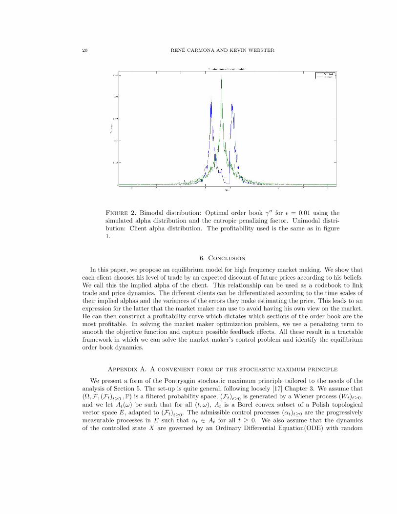
5.3. Interpretation. Figure 1 and Figure 2 illustrate what the market maker does:

(1) He tries to stick to a shape not too far away from µt, his client alpha distribution. This isto avoid feedback effects and associated errors on the price estimation.

(2) He also takes into account the profitability function mt, which leads him “to make a bighole” in the center of the distribution µt.

The combined effects lead to the familiar “double hump” shape of the order book, as seen in [18].Other consequences of the liquidity formula are

(1) In the limit where one client is perfectly intelligent of the price (ε → 0), the market makerplaces a Dirac mass on the order book. In particular, he only trades on profitable sectionsof the book.

(2) In the noise trade limit (ε → ∞), the market maker simply reproduces the client alphadistribution.

(3) If the return distribution of the asset is mean-reverting (which is not the case for optionswith maturities, for example), then so will µt and hence γt and ct. In the case of a Europeanoption, γ′′t converges to a Dirac at the payoff at maturity.


Figure 2. Bimodal distribution: Optimal order book γ′′ for ε = 0.01 using thesimulated alpha distribution and the entropic penalizing factor. Unimodal distri-bution: Client alpha distribution. The profitability used is the same as in figure1.

6. Conclusion

In this paper, we propose an equilibrium model for high frequency market making. We show thateach client chooses his level of trade by an expected discount of future prices according to his beliefs.We call this the implied alpha of the client. This relationship can be used as a codebook to linktrade and price dynamics. The different clients can be differentiated according to the time scales oftheir implied alphas and the variances of the errors they make estimating the price. This leads to anexpression for the latter that the market maker can use to avoid having his own view on the market.He can then construct a profitability curve which dictates which sections of the order book are themost profitable. In solving the market maker optimization problem, we use a penalizing term tosmooth the objective function and capture possible feedback effects. All these result in a tractableframework in which we can solve the market maker’s control problem and identify the equilibriumorder book dynamics.

Appendix A. A convenient form of the stochastic maximum principle

We present a form of the Pontryagin stochastic maximum principle tailored to the needs of theanalysis of Section 5. The set-up is quite general, following loosely [17] Chapter 3. We assume that(Ω,F , (Ft)t≥0 ,P) is a filtered probability space, (Ft)t≥0 is generated by a Wiener process (Wt)t≥0,

and we let At(ω) be such that for all (t, ω), At is a Borel convex subset of a Polish topologicalvector space E, adapted to (Ft)t≥0. The admissible control processes (αt)t≥0 are the progressivelymeasurable processes in E such that αt ∈ At for all t ≥ 0. We also assume that the dynamicsof the controlled state X are governed by an Ordinary Differential Equation(ODE) with random


coefficients valued in Rn:

dXt = ft(Xt, αt)dt (A.1)

where the coefficient f : (ω, t,X, a)→ ft(X, a) is Lipschitz in X uniformly in all the other variables.Assume an estimate of the form

|Xt| ≤ |X0|eCt (A.2)

where C is a constant. We also assume that f is continuously differentiable (i.e. C1) in X. Thecontroller’s objective function is given by

J(α) = E[∫ τ

0

jt(Xt, αt)dt+ gτ (Xτ )

](A.3)

where τ is a stopping time adapted to (Ft)t≥0 and j and g are random real-valued concave func-

tions which are C1 in X. Furthermore, we assume that j, g and τ are such that E [|gτ (Xτ )|] andE[∫ τ

0|jt(Xt, αt)|dt

]are finite and uniformly bounded from above. Next, we define the Hamiltonian

Ht(ω,X, a, Y ) = ft(ω,X, a)Y + jt(ω,X, a) (A.4)

for Y ∈ Rn and for each admissible control (αt)t≥0, the adjoint equation:

−dYt = ∂XHt(Xt, αt, Yt)dt− ZtdWt (A.5)

with Yτ = ∂Xg(Xτ ) and Zt such that E∫ τ

0|Zt|2dt < ∞. Under these conditions we have the

following result.

Theorem A.1 (Pontryagin’s maximum principle). Let α be an admissible control and X be theassociated state variable. Suppose there exists a solution (Y,Z) to the adjoint equation (A.5) suchthat

E[∫ τ

0

eCt|Zt|2dt]<∞, (A.6)

and the Hamitonian verifies for everyt ≥ 0

Ht(Xt, αt, Yt

)= maxa∈AtHt

(Xt, a, Yt

), a.s. (A.7)

and for every t ≥ 0, almost surely, the function

(X,α) → Ht(Xt, αt, Yt

)is concave, then α is an optimal control, that is, J(α) ≤ J(α) for all admissible α = (αt)t≥0.


Proof. If (Xt)t≥0 is the state associated to another admissible control (αt)t≥0, we have the chain ofrelationships:

E[gτ (Xτ )− gτ (Xτ )

]≤ E

[(Xτ − Xτ

)· Yτ]

(A.8)

= E[∫ τ

0

(−(Xt − Xt

)· ∂XHt(Xt, αt, Yt) +

(ft(Xt, αt)− ft(Xt, αt)

)· Yt)dt

](A.9)

≤ E[∫ τ

0

(Ht(Xt, αt, Yt)−Ht(Xt, αt, Yt) +

(ft(Xt, αt)− ft(Xt, αt)

)· Yt)dt

](A.10)

= E[∫ τ

0

(Ht(Xt, αt, Yt)−Ht(Xt, αt, Yt)−Ht(Xt, αt, Yt) +Ht(Xt, αt, Yt)

)dt

]− E

[∫ τ

0

(jt(Xt, αt)− jt(Xt, αt)

)dt

](A.11)

≤ −E[∫ τ

0

jt(Xt, αt)− jt(Xt, αt)

]. (A.12)

(A.8) stems from the concavity of g and terminal condition of Y . (A.9) follows from the dynamicsof Y and the relationship:

E[∫ τ

0

(Xt − Xt

)2

Z2t dt

]≤ 2X0E

[∫ τ

0

eCtZ2t dt

]<∞ (A.13)

which guarantees that the local martingale part is a martingale. (A.10) holds by the concavity ofthe Hamiltonian. (A.11) is just the definition of H. Finally, (A.12) is a consequence of the fact that

αt maximizes Ht(Xt, ·, Yt).

Appendix B. Derivation of the SPDE (4.16)

We give the main steps of the proof of Proposition 4.1. By independence of the common random-ness W and the idiosyncratic randomness (M i, αi0, ε

i)i≥1, we can freeze the randomness of W andwork after conditioning with respect to FW , the σ-algebra generated by W , without affecting theindependence properties of the idiosyncratic random variables. By independence of the M i, the αi0and εi, we have that, conditional on FW , the random variables

αit = αi0e−ρt +

∫ t

0

e−ρ(t−s)(νdWs + σdM i

s

)(B.1)

are iid and Gaussian. So if f ∈ C2 is such that f and its two derivatives have at most polynomialgrowth, given the assumption (4.17) on the joint distribution m of all the couples (αi0, ε

i), we canapply the law of large numbers and get:

limn→∞

1

n

n∑i=1

εif(αit) = E[ε1f(α1

t )∣∣FW ]

=

∫R3

εf

α0e−ρt +

∫ t

0

e−ρ(t−s)νdWs + σx

√∫ t

0

e−2ρ(t−s)ds

1√2πe−

x2

2 m(dα0, dε)dx

The other results can be derived directly from this explicit representation.


References

[1] A. Alfonsi, A. Fruth, and A. Schied. Optimal execution strategies in limit order books with general shapefunctions. Quantitative Finance, 10(2):143–157, 2010.

[2] R. Almgren and N. Chriss. Optimal execution of portfolio transactions. Journal of Risk, 3(2):5–39, 2000.

[3] R. F. Almgren. Optimal execution with nonlinear impact functions and trading-enhanced risk. Applied Mathe-matical Finance, 10(1):1–18, 2003.

[4] Y. Amihud and H. Mendelson. Asset pricing and the bid-ask spread. Journal of Financial Economics, 17(2):223–

249, 1986.[5] J. . Bouchaud, Y. Gefen, M. Potters, and M. Wyart. Fluctuations and response in financial markets: The subtle

nature of ’random’ price changes. Quantitative Finance, 4(2):176–190, 2004.[6] J. . Bouchaud, M. Mzard, and M. Potters. Statistical properties of stock order books: Empirical results and

models. Quant.Finance, 2(4):251–256, 2002.

[7] R. Cont, S. Stoikov, and R. Talreja. A stochastic model for order book dynamics. Operations research, 58(3):549–563, 2010.

[8] I. Csiszar. Information-type measures of difference of probability distributions and indirect observations, volume 2.

1967.[9] F. Delbaen and W. Schachermayer. The Mathematics of Arbitrage. Springer Verlag, 2010.

[10] M. B. Garman. Market microstructure. Journal of Financial Economics, 3(3):257–275, 1976.

[11] J. Hasbrouck. Empirical market microstructure. Oxford University Press, 2007.[12] T. G. Kurtz and J. Xiong. Particle representations for a class of nonlinear spdes. Stochastic Processes and their

Applications, 83(1):103–126, 1999.

[13] T. G. Kurtz and J. Xiong. Numerical solutions for a class of SPDEs with applications to filtering. Stochastics inFinite and Infinite Dimension, pages 233–258, 2000.

[14] A. S. Kyle. Continuous auctions and insider trading. Econometrica, 53(6):1315–1335, 1985.[15] P.A. Meyer. Probabilities and Potential. North-Holland Pub., 1966.

[16] A. Obizhaeva and J. Wang. Optimal trading strategy and supply/demand dynamics. Preprint, 2005.

[17] H. Pham. Continuous-time stochastic control and optimization with financial applications. Springer Verlag, 2008.[18] M. Wyart, J. . Bouchaud, J. Kockelkoren, M. Potters, and M. Vettorazzo. Relation between bid-ask spread,

impact and volatility in order-driven markets. Quantitative Finance, 8(1):41–57, 2008.

[19] I. Zovko and J. D. Farmer. The power of patience: A behavioral regularity in limit order placement. QuantitativeFinance, 2(5):387–392, 2002.

introduction - princeton universityrcarmona/download/fe/cw1.pdfmoreover, since liquidity providers...

Documents