NBER WORKING PAPER SERIES

INTERTEMPORAL PRICE DISCRIMINATION IN STORABLE GOODS MARKETS

Igal HendelAviv Nevo

Working Paper 16988http://www.nber.org/papers/w16988

NATIONAL BUREAU OF ECONOMIC RESEARCH1050 Massachusetts Avenue

Cambridge, MA 02138April 2011

We are grateful to Marciano Siniscalchi, and seminar participants for helpful comments. This researchwas funded by a cooperative agreement between the USDA/ERS and Northwestern University, butthe views expressed herein are those of the authors and do not necessarily reflect the views of the U.S.Department of Agriculture or the National Bureau of Economic Research.

NBER working papers are circulated for discussion and comment purposes. They have not been peer-reviewed or been subject to the review by the NBER Board of Directors that accompanies officialNBER publications.

© 2011 by Igal Hendel and Aviv Nevo. All rights reserved. Short sections of text, not to exceed twoparagraphs, may be quoted without explicit permission provided that full credit, including © notice,is given to the source.

Intertemporal Price Discrimination in Storable Goods MarketsIgal Hendel and Aviv NevoNBER Working Paper No. 16988April 2011JEL No. D43,E3,E30,L1,L13

ABSTRACT

We study intertemporal price discrimination when consumers can store for future consumption needs.To make the problem tractable we offer a simple model of demand dynamics, which we estimate usingmarket level data. Optimal pricing involves temporary price reductions that enable sellers to discriminatebetween price sensitive consumers, who anticipate future needs, and less price-sensitive consumers.We empirically quantify the impact of intertemporal price discrimination on profits and welfare. Wefind that sales: (1) capture 25-30% of the profit gap between non-discriminatory and third degree pricediscrimination profits, and (2) increase total welfare.

Igal HendelDepartment of EconomicsNorthwestern University2001 Sheridan RoadEvanston, IL 60208igal@northwestern.edu

Aviv NevoDepartment of EconomicsNorthwestern University2001 Sheridan RoadEvanston, IL 60208-2600and NBERnevo@northwestern.edu

1 Introduction

Consumers are heterogenous in many ways including preferences, income, transportation cost

and storage costs. Consumer heterogeneity generates incentives for firms to price discrim-

inate. When consumer types are unobservable firms rely on various screening mechanisms

to achieve separation. Empirically, we know little about the potential benefits from price

discrimination in actual settings, or how well various screening mechanisms work. Further-

more, the impact of price discrimination on welfare, especially in an oligopoly setting, is

theoretically unclear.

The goal of this paper is to empirically study the role of intertemporal price discrimina-

tion in storable goods markets. In these markets, temporary price reductions (sales) can be a

way to separate between consumers based on their ability to store. We estimate preferences,

and use the estimates to test whether sales can be driven by price discrimination. Next, we

evaluate the effectiveness of sales as a price discriminating tool relative to third-degree dis-

crimination, where the seller can identify the different consumer types and prevent arbitrage.

Finally, we assess the consequences of discrimination on consumer and total welfare.

In order to address these issues we need a model of pricing that is workable and consistent

with demand dynamics. A key computational and conceptual challenge in modelling the

sellers’ problem is the size of the state space. It is not clear how to reasonably model

the complex problem sellers face. Sellers’ profits, in principle, depend on the inventory

of each potential buyer. In which case, not only modeling the seller problem becomes very

complex, but also it is unreasonable to assume the seller can access and process such detailed

information. One could imagine solving the seller’s problem by assuming some sort of rule

of thumb or approximation to the optimal behavior. We explore an alternative which relies

on a simple dynamic demand model. The simplicity of the model helps in two ways. First,

demand is easy to estimate using market level data and computationally no more costly

than static demand estimation. Second, the proposed demand framework leads to a simple

solution to the sellers’ pricing problem. The model provides a clear delineation of what

sellers must observe to solve their problem, and makes the problem tractable.

The simplicity of the demand model is due to the storage technology: consumers store for

a pre-specified maximium number of periods. Characterizing consumer behavior does not

require solving the value function. The problem remains dynamic, but easy to solve. The

model is flexible enough to accommodate product differentiation, consumer heterogeneity

and endogenous consumption, while allowing for storability.

We estimate the demand model using store level scanner data for soft drinks and find

that consumers who store are more price sensitive than consumers who do not. This sug-

gests that firms would benefit from separating these groups, targeting storers with lower

2

prices. To evaluate profits and consumer surplus under different pricing regimes we use the

estimated demand, and respective first order conditions. Two benchmarks are considered.

One benchmark is non-discriminatory pricing. The other benchmark is third degree price

discrimination under the assumption of no arbitrage, namely, assuming sellers can target

different populations. Profits under third degree discrimination are a non-feasible upper

bound on gains from price discrimination. The target is not feasible because in practice

sellers cannot perfectly separate the different buyer types. We find that third degree price

discrimination would increase profits by 9-14% relative to non-discriminatory prices. Sales,

as a form of partial discrimination, enable sellers to capture around 24-30% of the potential

additional profits generated from discrimination.

The welfare implications of third degree price discrimination by a monopolist were studied

by Robinson (1933), and later formalized by Schmalensee (1981), Varian (1984) and Aguirre

et al. (2010) among others. The impact of discrimination on welfare is ambiguous. In

oligopoly situations there are virtually no (theoretical) welfare results. Therefore examining

the issues empirically is of particular interest. We find that total welfare increases. Sellers

are better off as are consumers who store. Consumers who do not store are worse off, but in

most cases their loss in more than offset by storers’ welfare gains.

Besides quantifying the impact of price discrimination there are other reasons to be

interested in our supply side analysis. There is a long tradition in Industrial Organization

of using demand estimates in conjunction with static first order conditions to infer market

power. Demand dynamics render static first order conditions irrelevant. A supply framework

consistent with demand dynamics is needed to infer market power. In addition, Macro and

Trade economists are interested in studying the pass through of exchange rates and monetary

shocks to consumer prices. To fully understand disaggregate micro level patterns one needs

a supply model that can be used to simulate the pass through.

Our paper is related to several strands in the literature. Numerous papers in Economics

and Marketing document demand dynamics, specifically, demand accumulation (see Blat-

tberg and Neslin (1990) for a survey of the Marketing literature). Boizot et al. (2001) and

Pesendorfer (2002) show that demand increases in the duration from previous sales. Hendel

and Nevo (2006a) document demand accumulation and demand anticipation effects, namely,

duration from previous purchase is shorter during sales, while duration to following purchase

is longer for sale periods. Erdem, Imai and Keane (2003), and Hendel and Nevo (2006b) esti-

mate structural models of consumer inventory behavior. Our demand model is motivated by

this literature but offers substantial computational savings and a tractable supply analysis.

Several explanations have been proposed in the literature to why sellers offer temporary

discounts. Varian (1980) and Salop and Stiglitz (1982) propose search based explanations

which deliver mixed strategy equilibria, interpreted as sales. Sobel (1984), Conlisk Gerstner

3

and Sobel (1984), and Pesendorfer (2002) present models of intertemporal price discrim-

ination in the context of a durable good (more recently used by Chevalier and Kashyap

(2011)), while Narasimhan and Jeuland (1985) and Hong, McAfee and Nayyar (2002) do so

for storable goods.

Our estimates show that sellers have an incentive to intertemporally price discriminate,

suggesting that sales are probably driven by discrimination motives. Incentives for sales are

similar to Narasimhan and Jeuland (1985) and Hong, McAfee and Nayyar (2002) but in a

somewhat different context. Hong et al. model an homogenous good sold in different stores,

under unit demand, and single unit storage. Since the interest in this paper is empirical we

need a framework amenable for demand estimation, that allows for product differentiation

and endogenous consumption and storage levels, depending on prices.

The abovementioned third-degree discrimination theoretical results (e.g., Robinson (1933),

Schmalensee (1981), and Aguirre et al. (2010)) apply to the intertemporal discrimina-

tion in our model, once we reinterpret demand during sale periods —following Robinson’s

terminology— as the weak demand, and demand during non-sale periods as the strong de-

mand.

Finally, our results relate to several papers in the empirical price discrimination litera-

ture. Shepard (1991) finds that, consistent with price discrimination motives, the price gap

between full and self service is higher at gas stations offering both levels of service relative to

the average difference between prices at stations offering only one type of service. Verboven

(1996) considers whether discrimination can explain differences in automobile prices across

European countries. Villas-Boas (2009) uses demand estimates and pricing (in the vertical

chain) to predict that banning wholesale price discrimination in the German coffee market

would increase welfare.

The paper proceeds as follows. In the next subsection we presents some motivating facts.

Section 2 presents a general, but non practical, model of demand and supply followed by our

simple model. Section 3 presents the estimation. Section 4 presents the application to soft

drinks.

1.1 Motivating Facts

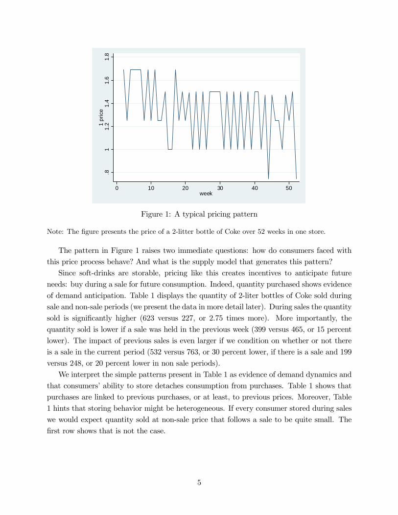
Figure 1 shows the price of a 2-liter bottle of Coke in a store over a year. The pattern is

typical of pricing observed in scanner data: regular prices and occasional sales, with return

to the regular price. With the exceptions of a short transition period, in any given 2-3 week

window there are two relevant prices: a sale price and a non-sale price. We note that while

sales are not perfectly predictable they are quite regular and frequent. Both these facts will

feed into our modeling below.

4

.81

1.2

1.4

1.6

1.8

1 p

rice

0 10 20 30 40 50week

Figure 1: A typical pricing pattern

Note: The figure presents the price of a 2-litter bottle of Coke over 52 weeks in one store.

The pattern in Figure 1 raises two immediate questions: how do consumers faced with

this price process behave? And what is the supply model that generates this pattern?

Since soft-drinks are storable, pricing like this creates incentives to anticipate future

needs: buy during a sale for future consumption. Indeed, quantity purchased shows evidence

of demand anticipation. Table 1 displays the quantity of 2-liter bottles of Coke sold during

sale and non-sale periods (we present the data in more detail later). During sales the quantity

sold is significantly higher (623 versus 227, or 2.75 times more). More importantly, the

quantity sold is lower if a sale was held in the previous week (399 versus 465, or 15 percent

lower). The impact of previous sales is even larger if we condition on whether or not there

is a sale in the current period (532 versus 763, or 30 percent lower, if there is a sale and 199

versus 248, or 20 percent lower in non sale periods).

We interpret the simple patterns present in Table 1 as evidence of demand dynamics and

that consumers’ ability to store detaches consumption from purchases. Table 1 shows that

purchases are linked to previous purchases, or at least, to previous prices. Moreover, Table

1 hints that storing behavior might be heterogeneous. If every consumer stored during sales

we would expect quantity sold at non-sale price that follows a sale to be quite small. The

first row shows that is not the case.

5

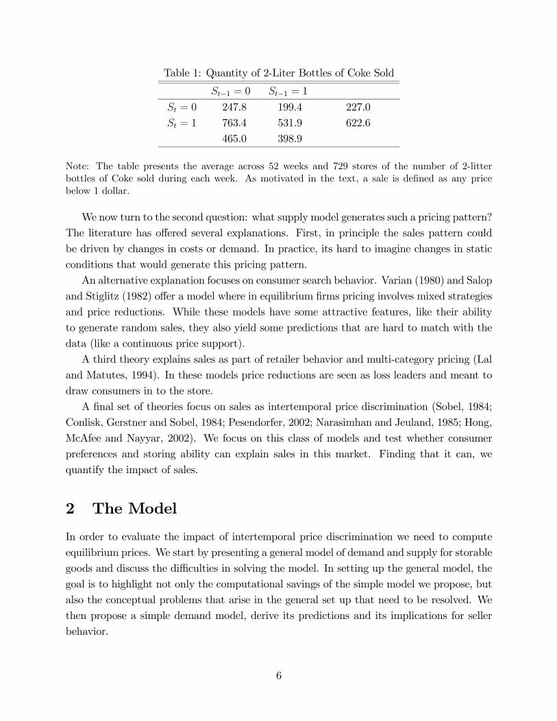
Table 1: Quantity of 2-Liter Bottles of Coke Sold

−1 = 0 −1 = 1

= 0 247.8 199.4 227.0

= 1 763.4 531.9 622.6

465.0 398.9

Note: The table presents the average across 52 weeks and 729 stores of the number of 2-litter

bottles of Coke sold during each week. As motivated in the text, a sale is defined as any price

below 1 dollar.

We now turn to the second question: what supply model generates such a pricing pattern?

The literature has offered several explanations. First, in principle the sales pattern could

be driven by changes in costs or demand. In practice, its hard to imagine changes in static

conditions that would generate this pricing pattern.

An alternative explanation focuses on consumer search behavior. Varian (1980) and Salop

and Stiglitz (1982) offer a model where in equilibrium firms pricing involves mixed strategies

and price reductions. While these models have some attractive features, like their ability

to generate random sales, they also yield some predictions that are hard to match with the

data (like a continuous price support).

A third theory explains sales as part of retailer behavior and multi-category pricing (Lal

and Matutes, 1994). In these models price reductions are seen as loss leaders and meant to

draw consumers in to the store.

A final set of theories focus on sales as intertemporal price discrimination (Sobel, 1984;

Conlisk, Gerstner and Sobel, 1984; Pesendorfer, 2002; Narasimhan and Jeuland, 1985; Hong,

McAfee and Nayyar, 2002). We focus on this class of models and test whether consumer

preferences and storing ability can explain sales in this market. Finding that it can, we

quantify the impact of sales.

2 The Model

In order to evaluate the impact of intertemporal price discrimination we need to compute

equilibrium prices. We start by presenting a general model of demand and supply for storable

goods and discuss the difficulties in solving the model. In setting up the general model, the

goal is to highlight not only the computational savings of the simple model we propose, but

also the conceptual problems that arise in the general set up that need to be resolved. We

then propose a simple demand model, derive its predictions and its implications for seller

behavior.

6

2.1 Demand and Supply with Storable Products

Assume consumer has preferences at time given by a utility function (q; ) where

q = [1 2 ]0 is the vector of quantities consumed of the varieties of the product, ,

is the quantity consumed of a nummeraire, and is a vector of consumer specific time

varying parameters. We denote (q) ≡ (q; ) Consumers can store for future

consumption at costs (i), where i is a vector of dimension of the inventory of all brands.

Consumers know current prices and the distribution of prices at period +1 (p|) where

p is a vector of dimension of prices and is the history up to

The consumer’s problem in each period is to choose purchases, x and consumption,

q of each brand to

∞X=0

E [+(q+ + )− (i+)|] (1)

s.t. p0+x+ ++ ≤ + and i+ = i+−1 + x+ − q+

where is the discount factor, and is the consumer’s income at period . The expectation

is taken with respect to future prices as well as uncertain future needs. Consumers trade off

purchasing today, if prices are low, and paying a storage cost. Market demand, X(p)

is given by aggregation across consumers who solve the problem in equation (1).

The seller’s problem is to choose a series of prices to maximize the discounted flow of

expected profits, () For simplicity, we assume the seller is a monopolist who can commit

to future prices, and produces all varieties at a constant marginal cost, . Then the seller’s

problem is to choose prices, p, to maximize

∞X=0

E [(p+)|] =∞X=0

E [(p+ − c+)0X+ (p+ +)|] (2)

The expectation is taken with respect to future demand shocks that impact both the

functional form of X+ and the history in future periods, + Note, that if demand is

static, X(p) = X(p), then the pricing problem is static.

2.1.1 Equilibrium and the Information Structure

The equilibrium prices are determined by the interaction between the problems outlined in

equations (1) and (2). Regardless of what is computationally feasible we would like to discuss

what information can be reasonably assumed to be available and likely to be used. What do

players’ strategies depend on in these markets?

7

Pricing, in principle, may depend on the inventory held by each of the buyers in the

population as well as their preference shocks. Given pricing, consumers purchasing decisions

would depend on such information as well, should it be available to them. Howvere, in-

ventories, which depend on previous consumption, are private information. Past purchases

could be used to infer individual preference, and perhaps to estimate the current inventory

holdings of each buyer. While some individual information might be available for customers

that use loyalty cards, the informational and computational burden of processing such in-

formation seems enormous. Therefore, its umreasonable to assume that frims condition on

this information. Unable to track individual purchases over time, sellers might still find it

useful to condition pricing on the distribution of past quantities sold or, as a proxy, on total

quantity sold. However, it raises the issue of whether buyers and competitors have access to

such information.

A more realistic assumption is that strategies depend on public information, namely,

prices. Hong, McAfee and Nayyar (2002) provide a model in which (observable) past prices

suffice to infer past purchases. In their model preferences are deterministic and identical, the

distribution of holdings can be inferred from purchases. Thus, the starting inventory and

the identity of those holding inventory is known at any point in time. With the empirical

goal in mind of estimating preferences, we would like a more general model, than Hong et

al., that allows for: 1) differentiated products, 2) consumption and the quantity stored to

depend on price and 3) non-deterministic demand.

2.2 A Simple Demand Model

In this section we propose a model that accommodates the empirical requirements, yet prices

are a sufficient statistic for the state. Although simple, it delivers an empirical framework for

estimation. We first present the main assumptions, and then discuss the implied purchasing

patterns.

2.2.1 The Setup

First, we assume that there is heterogeneity in the willingness or ability to store.

Assumption A1: a proportion of consumers do not store.

In the setup of Section 2.1 this would arise endogenously if a fraction of the consumers

have storage costs that make it unprofitable to store. Therefore, one can view A1 as an

assumption on the distribution of storage costs.

We allow storers and non-storers to have different preferences. Let (q) and

(q)

be the preferences of the representative storing and non-storing consumer, respectively. For

8

simplicity we assume preferences are quasi-linear, i.e.,

(q) = (q) + and

(q) = (q) + (3)

We index preferences by to allow for changing demand; we assume that consumers know

needs at least periods in advance. Preferences could reflect an aggregate consumer, assum-

ing the household level preferences are of Gorman form and yield an aggregate consumer.

Alternatively, preferences could represent explicit aggregation over individual households (for

example, as in Berry, Levinsohn and Pakes, 1995).

Preference heterogeneity will be an important determinant of seller behavior. It is an

empirical matter if, and how, preferences of the types differ. We can, in principle, find that

the proportion of either type is zero or that preferences are identical.

Absent storage, purchases equal consumption, thus, consumers’ aggregate demand by

type is

q = (p) and q

= (p) (4)

where (·) is the demand function implied by maximizing the utility in (3).With storage, purchases and consumption need not coincide. In order to predict storers’

purchases we make the following assumptions:

A2 (storage technology): storage is free, but inventory lasts for only periods (fully

depreciates afterwards).

Taken literally the assumption implies perishability. For example, = 1 fits products

that would not last more than two weeks (the period of purchase and the following). For

products with longer life a higher would fit. An alternative interpretation of the assumption

is contemplation; while the product may last longer, at the store the buyers only considers

purchasing for periods ahead. The assumption implies simple dynamics. In the inventory

problem defined in Section 2.1, the consumer and the researcher need to keep track of how

much is left in storage in different states. As shown in the next section this is not the case

here. In addition, the assumption detaches the storage decision of different products. In

the problem in Section 2.1 the storage cost is a function of the inventory of all varieties.

Under A2 effective prices, of the other products, are a sufficient statistic for quantity in

storage. Effective prices, defined later, are the opportunity cost of period consumption.

Moreover, effective prices are public information. Thus, the assumption not only eases

demand estimation but also helps formulate the sellers’ problem.

Finally, we assume the following about prices expectations.

A3 (perfect foresight): consumers have perfect foresight regarding prices periods

ahead.

9

As we will see below with perfect foresight the consumer problem becomes particularly

simple. One may worry that perfect foresight is restrictive, thus, invalidating demand es-

timates and perhaps an inadequate assumption to study sellers behavior. It turns out the

perfect foresight assumption fits the supply model under seller commitment. However, we

will also consider an alternative assumption:

A3’ (rational expectations): consumers hold rational expectations about future prices

We can solve the model under either perfect foresight (A3) or rational expectations (A3’)

for low . We present estimates under both assumptions. For low the results are similar.1

It is much easier to allow for 1 under A3.

2.2.2 Purchasing Patterns

We now derive the purchasing patterns implied by A1-A3. For ease of exposition we ignore

discounting. The application involves weekly data, and therefore discounting does not play

a big role. In order to insure a solution to the dynamic problem we focus on a finite horizon,

up to period .

Aggregate purchases are the sum of the purchases of the two types of consumers:

(p− p+ ) = (p) +

(p− p+ ) (5)

where (p) are purchases by storers. Non-storers behave according to (4).

Storers’ purchasing patterns are determined as follows. Their objective function is to

maximize the sum of utility in the periods subject to a budget constraint and the storing

constraints. Formally, they solve

X=0

E( (q) +) subject to

X=0

(p0x +) ≤X=0

and q ≤ x −−1X=0

(x − q − e)

where x is the vector of purchases, and e is the vector of unused units that expire in period

. We have in mind items on which expenses are small relative to wealth so that 0

1We believe the reason estimates are similar is that there are well defined sales and non-sale prices. If

consumers do not know future prices, but there are two clear price ranges then they purchase for storage on

sale, and never store at non-sale prices. In other words, under the two price range assumption knowledge

of future prices is not needed to generate the same storing behavior that arises under perfect foresight.

Although in the application there are more than two prices, in Figure 1 one can see a clear distinction

between sale and non-sale prices.

10

for all , therefore income effects or liquidity constraints in any particular period do not play

a role.

Assumptions A2 and A3 imply that storers’ solve for consumption periods in advance.

Storage allows them to buy each product consumed at at the lowest of the preceding

prices. To write down the problem, we define the effective price of product in period as

= min{ −} (6)

where = min{ } is the number of periods back in which period consumption could

have been purchased. The constraint ≤ (in the definition of ) takes care of the initial

periods, namely, purchases before period 0 are not feasible.

Using p which denotes the vector of period effective prices, the problem of the storing

consumer becomes

X=0

E( (q) +) subject to (peft0q +) ≤

The optimization of the storer is a sequence of static optimization problems solved periods

in advance, and replacing prices by effective prices. Optimal consumption in period is

q = (p

eft ). The dynamics are taken care simply by replacing prices by effective prices.

The storage of a product affects the purchases and consumption of all other products

exclusively through its effective price. To see that suppose product was purchased during

a sale for consumption in subsequent periods. Demand for all other products is naturally

affected by the fact that product is in the pantry waiting to be consumed. How do

inventoried units of affect demand for −? Since was known at the time of purchasingall varieties to be consumed at period the impact is fully captured by plugging the effective

price of consuming in those later periods.

Having solved the optimal consumption path we need to predict purchases. In period

the consumer might purchase for as well as for some or all of the following periods. For

= 0 purchases at time for consumption at time + equal either 0, if +,

or (absent ties in effective prices) +(p

eft+r), if =

+

However, since prices may repeat themselves between periods − and consumers are

indifferent when to purchase. We break the tie by assuming that buyers purchase immedi-

ately when the price is below a threshold, and wait otherwise. Namely, for

consumers buy right away, while for ≥ consumers buy in the last opportunity in which

prices equal . Threshold triggers action. A possible rationale for this —arbitrary— tie-

breaking rule is a little uncertainty about either going to the store or about future prices.

As a practical matter we can use median price as the threshold.

11

The tie breaking rule requires a little more notation. Define = min{argmin≤{p p−}}and = max{argmin≤{p p−}} These are the first and last time is charged inthe − to period, respectively.

Period purchases are:

(p− p+ ) =

X=0

+(p

−+)1{(( = )∩( ))∪(( = )∩( ≥ ))}

(7)

where +(·) is static demand defined by (4). The indicator function takes care of two

requirements. First, we only want to purchase at time for consumption in period + if

= +, that is, if price is as good as any other price between + − and +

Second, the indicator takes care of breaking ties. Purchases take place at only if is the

first event in which a price below the threshold is offered, or the last, if the price is above

the threshold.

2.2.3 Predicted Behavior for T=1

We now spell out what equation (7) implies in the case of = 1. Focusing on = 1, while

just a private case, serves two purposes. First, it will help clarify our estimating equations,

highlighting how the model is identified from the data. Second, it prepares the ground to

show how the model works under rational expectations.

Equation (7) dictates when consumers buy for future consumption, in this case for +1.

We will denote a period as either a non-sale period, , or a sale period, . Sale periods are

periods in which the storing consumer buys for future consumption, that is for product

period , when +1. A non-sale period, , is one which +1. If = +1

then the period is classified as a sale if and non sale otherwise.

Consumers who store, purchase for storage at , and never store at When they store,

they do so for one period, and their purchases are dictated by (4). Thus, to predict consumer

behavior we only need to define 4 events (or types of periods): a sale preceded by a sale

(), a sale preceded by a non-sale (), a non-sale preceded by a sale (), and two

non-sale periods ().

Assume for a second that only product can be stored. Given assumptions A1-A3 storers’

purchases at time are given by

(p−1pp+1) =

⎧⎪⎪⎪⎨⎪⎪⎪⎩( −)

0

( −)

0

+

0

0

+1( −+1)

+1( −+1)

in

(8)

12

where () is the static demand of storers (defined in (4)).

At high prices there are no incentives to store, in which case purchases equal either:

consumption, given by (), or zero, if there was a sale in the previous period (i.e., in

consumption is out of storage). During sales preceded by a non-sale period purchases are

for current consumption as well as for inventory. During periods of sale preceded by a sale,

current consumption comes from stored units, so purchases are for future consumption only,

and the purchases equal +1( −+1) Notice the difference in the second argument of

the anticipated purchases relative to purchases for current consumption (e.g., vs )

Purchases for future consumption take into account the expected consumption of products

−When all products are storable accounting for storability is immediate. The way to

incorporate the dynamics dictated by storage is to consider the effective cost (or price) of

consumption, which does not necessarily coincide with current price. In other words, if −is purchased on sale for future consumption, its effective future price,

−+1 is its current

(sale) price since the product will be stored today for consumption tomorrow. For example,

consider the event (product is not on sale at nor at − 1) and assume that product− was on sale at − 1 (but is not on sale at ). The demand from consumers who stored

is (

−) instead of

( −). A similar adjustment is needed in every state, to

account for consumption out of storage.

There are two important implications of equation (8) for estimation. First, when we

estimate the model we will use the states to scale demand up or down, but as equation (8)

suggests we will use the actual prices for estimation. The definition of the and is used

to define the state not to modify prices: prices are not restricted to take on two values and

can take on any value

Second, we can see from equation (8) that contemporaneous prices of other products

are the wrong control in the estimation. Controlling for current price generates a bias in

the estimated cross price effect. In an inventory model, the effective or shadow price is a

complicated creature that requires solving the value function. In our framework, for = 1

effective prices are just the minimum of current and previous prices.

Allowing for larger in the estimation is immediate. Equation (8) requires adjustment

to reflect that consumers can anticipate for longer periods ahead, as reflected in (7), basi-

cally rescaling up in case of anticipated purchases, and rescaling demand down, in case of

consumption out of storage. Moreover, effective prices are the minimum of the previous

periods. Basically, period consumption is the static demand based on peft while purchases

take place at the time the effective price is charged.

13

2.2.4 Rational Expectations

We now explore demand under A3’, of rational expectations, while continuing to assume A1

and A2. We will also focus on the = 1 case. Under these assumptions equation (5) is still

valid in the single product case (i.e., if other products are either not present or are sold at

a constant price) but we need an appropriate classification of and periods

Naturally, we cannot define a sale based on + 1 prices, which are not yet known (ab-

sent perfect foresight). Given the distribution of future prices, as shown in Hong et al.

(2002) and Perrone (2010), there is a threshold below which the good is purchased for future

consumption. We thus define sale and non-sale periods based on the price thresholds.

We will classify the periods of high prices as non-sale and low prices as sales. At high

prices buyers do not have an incentive to store, denote them as periods. During a sale

period, consumers have an incentive to store, even if some sales are deeper than others.

Thus, rational expectations and unrestricted price support work fine in the single product

case.2

When more than one product is storable the analysis involves the following issue. At

the time of purchasing product the (effective) prices of other products may not be known.

They would be known, for example, if the other products are on sale, in which case the

effective price is the current sale price. In general, when some other products are not on

sale, the consumer has to purchase product under uncertain − prices. Thus in period

storers chose +1 to maximize

{+1(+1q∗−+1(p−+1 +1))− +1 − q∗−+1(p−+1 +1)0p−+1}

where expectation is taken with respect to the distribution of − prices. q∗−+1(p−+1 +1)represents optimal − consumption in +1 given price realizations and pre-stored quantitiesBasically, at the consumer chooses product purchases knowing − consumption is con-tingent on the eventual − price.With a general price support the problem is solvable but it can be tedious since it requires

solving for q∗ for each point in the support of prices. The computation is much easier(especially for a small number of products) if we assume a two price support: and

For

example, suppose Coke is on sale and Pepsi is not, the consumer has to decide how much

Coke to purchase for +1 knowing Pepsi’s price at +1 may end up at one of two different

levels. The demand for Coke involves the solution of three first order conditions for: ,

2The only minor subtlety is whether consumers that stockpiled buy additional units should the realized

price be lower than the preceding price. It is possible that consumers purchase additional units given the

low price, or that they pay no attention to products in categories for which they already stored (they do not

even go through that aisle). Equation (5), as written, assumes the latter, but both options can be handled.

14

Coke purchase at for consumption at + 1 , Pepsi consumption at + 1 if Pepsi ends

up being on sale, and Pepsi consumption absent a sale.

While the two price support may come handy in the estimation of the rational expecta-

tions model, as we now explain, the model can still be estimated with an unrestricted price

distribution. Notice that only in some states predicted behavior requires knowledge of future

prices. For example, if both products are in demand does not depend on future prices.

In those states where predicted demand does not depend on future prices the predicted

behavior as explained in the previous section is still valid, and can be used in the estimation

under rational expectations. It turns out that in the 2 goods case, 10 of the 16 states

(composed of the cross product of the 4 states of each good) predicted purchases of each

product are the same under both expectations assumptions. In total only 2 out of the 16

states involve behavior that differs for both products. Thus, a way to estimate the model

under rational expectation, without incurring additional computation costs and without

the two price assumption, is to restrict the sample to periods where demand under both

expectations assumptions coincide. We elaborate on this below.

2.3 Seller Behavior

We start by considering a monopolist facing a population of non-storers and storers with

static demands given by () and (). We drop the time subscript, but it is immediate

to allow for changing demand. Marginal cost is . Let ∗ and ∗ be the prices that

maximize —static— profits from separately selling to the populations of storers and non-

storers, and ∗ the monopoly price of a non-discriminating monopolist facing the whole

population, composed of non-storers and storers. ∗ maximizes (() +())(− )

Denote ∗ = ((∗) +(∗))(

∗ − )

2.3.1 Two-period problem

We initially consider optimal prices in a two period set-up. Storability may enable price

discrimination if the seller would like to target storers with a lower price. Once storers

purchase for future consumption the seller can target non-storers with higher prices.

In some cases a constant price might be optimal. It is, for example, if ∗ ≤ ∗ On theother hand, suppose the seller charges in the first period and ∗ in the second period, for

some ∗ ∗ Denote profits from { ∗} as:

() = (() + 2())(− ) +(∗)(

∗ − )

15

The first term represents variable profits during sales, targeting storers who purchase for two

periods, and non-storers for one period. The last term represents profits from non-storers,

during non-sale periods. If

() 2∗ (9)

for some ∗ ∗ then the pair { ∗} does better than constant prices. Since the

best constant price is ∗, the above inequality guarantees all other constant prices do worse

than the proposed price pair. It is an empirical matter whether constant or increasing prices

are profitable. It depends on whether — using Robinson (1933)’s terminology — non-storers

are the strong market while storers the weak market.

We assume throughout the concavity of objective functions. Thus assuming condition (9)

holds then an increasing price sequence is optimal and the prices and ∗ are determined

by the solution to the following first order conditions:

∗ = − (∗)()

|=∗

(10)

= − () + 2()(()+2())

|=

2.3.2 Multiple-period problem

In a longer horizon we need to show that the price sequence proposed in the previous section

is feasible, and that no other price sequence does better. Consider horizons of length 2.

It is immediate to see that for any ≤ +1 the analysis of the previous section is still valid,

with optimal prices being for one period -to supply storers- followed by ∗ afterwards.

As long as the horizon is no longer than the storing period the seller clears storers out of the

market and then targets non-storers.

In longer horizons, +1 —if discrimination is profitable- cyclical prices are optimal.

The simplest case to consider is = 1; the analysis is similar for larger . We still assume

the monopolist can commit to future prices; we later argue that the same predictions arise

absent commitment, and under duopoly with commitment.

The monopolist maximizes profits

X=1

(|−1) =X=1

( −1 +1)( − )

where ( −1 +1) is given by 5. As before, we assume a finite horizon to avoid aninfinite sum due to the lack of discounting. The maximization boils down to picking a

sequence of prices, such that if −1 ≤ storers stockpile for future use.

16

Proposition 1 Under condition (9) optimal pricing involves cycles of followed by with

∗ = ∗

Proof. First consider the last two periods in isolation. Under condition 9 optimal prices

are followed by

Now look at a 4-period problem. The proposed cycle is feasible and attains twice the

profits of the two period problem. To see it is feasible notice that the candidate prices do not

generate storage between periods 2 and 3. Absent a link between period 2 and 3, consumers

behave as prescribed in each independent cycle (the first cycle is periods 1 and 2, the second

is periods 3 and 4).

It remains to be shown that no other price sequence is more profitable. First notice that

for any price sequence with 2 3 to be optimal it has to be our candidate [, , ].

Since 2 3 implies no storage in period 2, thus the two cycles are detached. The solution

to the detached problems involves followed by in each part.

It remains to rule out price sequences that involve storing in period 2, i.e., sequences

with 2 ≤ 3 If 2 ≤ 3 consumers store in period 2. Having purchased for period three

consumption in period two, in period three storers would only purchase for period four

consumption, and they would do so only if 3 ≤ 4 Suppose that indeed storers purchase in

period three for period four consumption. Since storers are absent in period four, the optimal

4 is while the best third period price is ∗ In the alternative case, in which storers do

not purchase in period three the optimal price on period three is followed by ∗ in period

four, since in the last period all customers are present (and there are no further purchases

for storage). Lets go back to the first two periods. There are two cases to consider, either

storers store in period one or they do not. If they store the only candidate for first period

price is , moreover, in period two they store for period three, thus the optimal price is ∗.

If they do not store in period one the optimal first period price is ∗ while the second

period optimal price is Thus, the optimal prices in the first two periods (given storage

between periods two and three) are: {∗ } or { ∗} followed by { ∗} or {∗ }in periods three and four. Either way profits amount to 2∗+() which by condition

9 is lower than 2(). Thus, the cycling prices do better than any other price sequence

in the four period problem.

It is interesting to notice that the cycle delivers discrimination twice, while the best

alternative pricing that links periods achieves once the discriminating profit level and for

two periods the non-discriminating profit level. Cycling prices maximize the times the seller

discriminates across buyers.

We can keep adding two-periods at a time and apply the same reasoning. The cycle is

feasible, and optimal assuming no storage between cycles. On the other hand, a sequence

that induces storage between cycles, as above, fails to exploit discrimination at least once.

17

Finally, we need to consider odd . It is easy to see that as we go from two to three

periods the best the seller can get is ∗ + () namely, one event of discrimination

plus a non-discriminating profit flow. The same is true for any -long horizon.

The proposed sale cycle leads to a flow profit (per two-period cycle) of () The

prediction is similar to Narasimhan and Jeuland (1985), which shows that cyclical pricing

(sales) help sellers intertemporally price discriminate when buyers with more intense needs

have more limited storage.

It is not difficult to show that the non-commitment solution coincides with the commit-

ment solution. The proof is a little tedious as it involves many cases, but roughly consider

what the possible deviation are. Lowering prices on a non-sale period is of no benefit, while

raising during a sale period does not help either (since it eliminates a discrimination event).

2.3.3 Duopoly

In the context of our application there is more than one manufacturer. We show that in the

commitment equilibrium both sellers charge cycling prices.

Consider firm taking as given firm ’s cycling prices. Since storers always purchase

good at the sale price, their demand is ( ) namely, it is the same in every period

regardless of the current price of product . In contrast, the non-storer’s demand ( )

depends on the contemporaneous price of product

Define non-discriminating profits by firm for each of the two prices charged by as:

∗(). We can now modify 9 for the duopoly case. The following is a sufficient condition

for discrimination to be profitable in a two-period set up:

( (

) + 2

( ))( − ) + ( )( − ) ∗() + ∗() (11)

Condition (11) says that in a two-period problem firm taking as given ’s low-high

price sequence, gains from intertemporal price discrimination. Namely, best responds

using cycling prices.

The same reasoning used to show that cycles are optimal for the monopolist in a longer

horizon, applies to the duopolist problem as well.3

3There is an additional issue, the timing of the sales. It is possible that non-coincidental cycles are more

profitable than coincidental sales. The issue does not arise in a two-period set up since there is no point of

having a sale in the second period. We abstract for the moment from the timing issue, that could arise in a

longer horizon, a condition like 11 would determine optimal timing.

18

3 Data and Estimation

3.1 Data

The data set we use was collected by Nielsen and it includes store-level weekly observations

of prices and quantity sold at 729 stores that belong to 8 different chains throughout the

Northeast US, for the 52 weeks of 2004. We focus on 2-liter bottles of Coke, Pepsi and store

brands, which have a combined market share of over 95 percent of the market.

There is substantial variation in prices over time and across chains. A full set of week

dummy variables explains approximately 20 percent of the variation in the price in either

Coke or Pepsi, while a full set of chain dummy variables explains less than 12 percent of

the variation.4 On the other hand, a set of chain-week dummy variables explains roughly 80

percent of the variation in price. Suggesting similarity in pricing across stores of the same

chain (in a given week), but prices across chains are different. It seems that all chains charge

a single price each week. However, three of the chains appear to define the week differently

than Nielsen. This results in a change in price mid week, which implies that in many weeks

we do not observe the actual price charged just a quantity weighted average. In principle we

could try to impute the missing prices. Since this is orthogonal to our main point we drop

these chains.

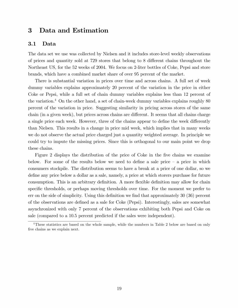
Figure 2 displays the distribution of the price of Coke in the five chains we examine

below. For some of the results below we need to define a sale price — a price in which

consumers stockpile. The distribution seems to have a break at a price of one dollar, so we

define any price below a dollar as a sale, namely, a price at which storers purchase for future

consumption. This is an arbitrary definition. A more flexible definition may allow for chain

specific thresholds, or perhaps moving thresholds over time. For the moment we prefer to

err on the side of simplicity. Using this definition we find that approximately 30 (36) percent

of the observations are defined as a sale for Coke (Pepsi). Interestingly, sales are somewhat

asynchronized with only 7 percent of the observations exhibiting both Pepsi and Coke on

sale (compared to a 10.5 percent predicted if the sales were independent).

4These statistics are based on the whole sample, while the numbers in Table 2 below are based on only

five chains as we explain next.

19

01

02

03

0P

erc

ent

.5 1 1.5 2Price of Coke

Distribution of the Price of Coke

Figure 2: The Distribution of the Price of Coke

Note: The figure presents a histogram of the distribution of the price of Coke over 52 weeks in 729

stores in our data.

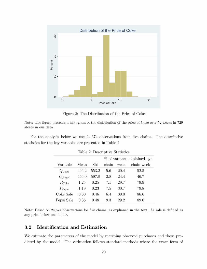
For the analysis below we use 24,674 observations from five chains. The descriptive

statistics for the key variables are presented in Table 2.

Table 2: Descriptive Statistics

% of variance explained by:

Variable Mean Std chain week chain-week

446.2 553.2 5.6 20.4 52.5

446.0 597.8 2.8 24.4 46.7

1.25 0.25 7.1 29.7 79.9

1.19 0.23 7.5 30.7 79.8

Coke Sale 0.30 0.46 6.4 30.0 86.6

Pepsi Sale 0.36 0.48 9.3 29.2 89.0

Note: Based on 24,674 observations for five chains, as explianed in the text. As sale is defined as

any price below one dollar.

3.2 Identification and Estimation

We estimate the parameters of the model by matching observed purchases and those pre-

dicted by the model. The estimation follows standard methods where the exact form of

20

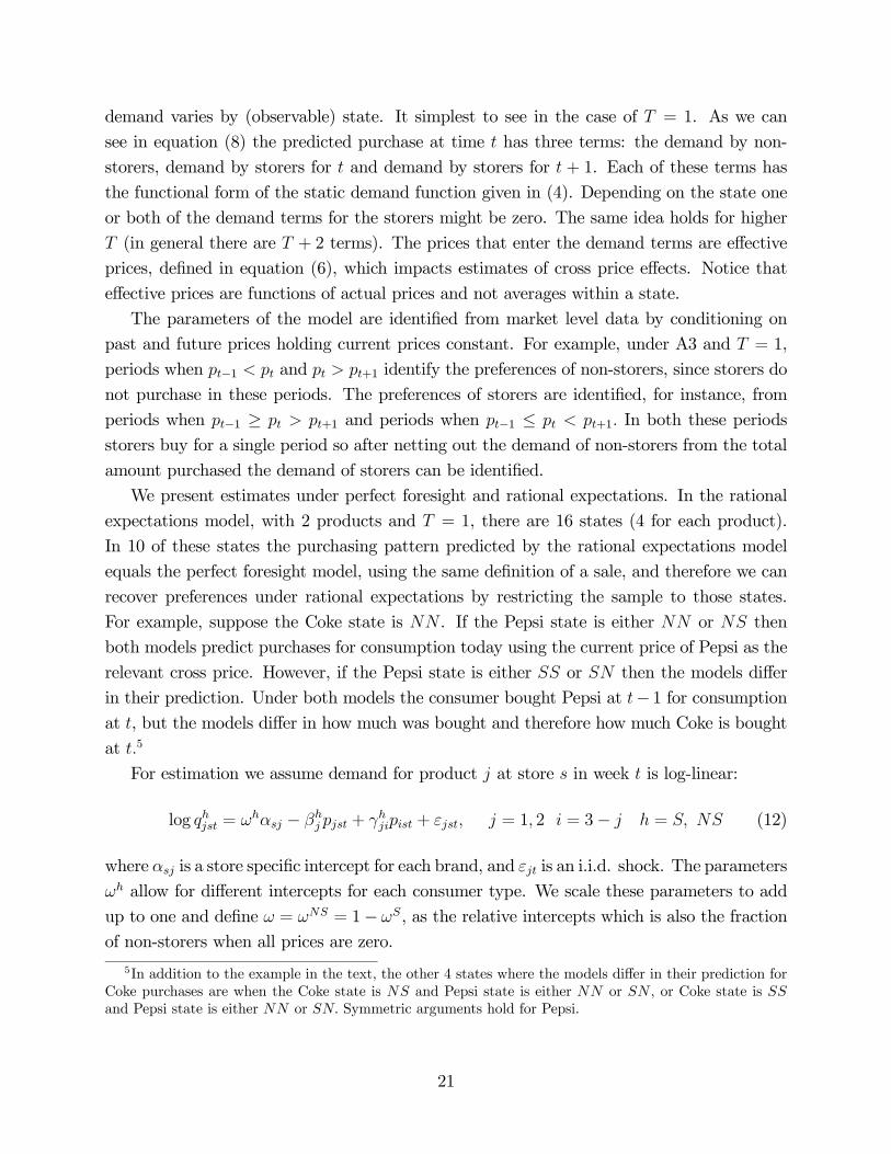
demand varies by (observable) state. It simplest to see in the case of = 1. As we can

see in equation (8) the predicted purchase at time has three terms: the demand by non-

storers, demand by storers for and demand by storers for + 1. Each of these terms has

the functional form of the static demand function given in (4). Depending on the state one

or both of the demand terms for the storers might be zero. The same idea holds for higher

(in general there are + 2 terms). The prices that enter the demand terms are effective

prices, defined in equation (6), which impacts estimates of cross price effects. Notice that

effective prices are functions of actual prices and not averages within a state.

The parameters of the model are identified from market level data by conditioning on

past and future prices holding current prices constant. For example, under A3 and = 1,

periods when −1 and +1 identify the preferences of non-storers, since storers do

not purchase in these periods. The preferences of storers are identified, for instance, from

periods when −1 ≥ +1 and periods when −1 ≤ +1 In both these periods

storers buy for a single period so after netting out the demand of non-storers from the total

amount purchased the demand of storers can be identified.

We present estimates under perfect foresight and rational expectations. In the rational

expectations model, with 2 products and = 1, there are 16 states (4 for each product).

In 10 of these states the purchasing pattern predicted by the rational expectations model

equals the perfect foresight model, using the same definition of a sale, and therefore we can

recover preferences under rational expectations by restricting the sample to those states.

For example, suppose the Coke state is . If the Pepsi state is either or then

both models predict purchases for consumption today using the current price of Pepsi as the

relevant cross price. However, if the Pepsi state is either or then the models differ

in their prediction. Under both models the consumer bought Pepsi at − 1 for consumptionat , but the models differ in how much was bought and therefore how much Coke is bought

at 5

For estimation we assume demand for product at store in week is log-linear:

log = − + + = 1 2 = 3− = (12)

where is a store specific intercept for each brand, and is an i.i.d. shock. The parameters

allow for different intercepts for each consumer type. We scale these parameters to add

up to one and define = = 1− , as the relative intercepts which is also the fraction

of non-storers when all prices are zero.

5In addition to the example in the text, the other 4 states where the models differ in their prediction for

Coke purchases are when the Coke state is and Pepsi state is either or , or Coke state is

and Pepsi state is either or Symmetric arguments hold for Pepsi.

21

We also experimented with a linear demand specification. In general, the demand results,

such as the difference between the static and dynamic model and the differences between

storers and non-storer, are similar. However, in the linear model predicted demand can be

negative (specially storers’ demand at a high price). The log-linear specification avoids the

negativity problem by imposing an asymptote to zero consumption as price increases.

We estimate all the parameters by non-linear least squares. We minimize the sum of

squares of the difference between the observed purchases and purchases predicted by the

model. We present the exact estimating equations in the Appendix. We should stress that

in all cases we use actual prices: the definition of sales is used to define the states but in

no way do we modify or average prices within state. In principle, we could use instrumental

variables to allow for correlation between prices and the econometric error term. However,

we do not think correlation between prices and the error term is a major concern in the

example below. To obtain the exact estimating equations we combine equations (5) and

(12), and allow for store fixed effects. To account for the store level fixed effects we de-

mean the data, which makes all the parameters enter the equations non-linearily. Still the

estimation is quite straightforward. We show in the Appendix how to modify the estimating

equation to account for the fixed effects.

4 Results

4.1 Demand Estimates

The estimation results are presented in Tables 3 and 4. The different columns present

estimates under alternative assumptions. In all cases the dependent variable is the (log of

the) number of 2-liter bottles of Coke or Pepsi sold in a week in a particular store. All

regressions include store fixed effects as well as the price of the store brand.

4.1.1 Main Results

The first two columns in Table 3 display estimates from a static model. The rest of the

columns present estimates from the dynamic model under different assumptions. In all cases

we assume = 1 and allow for different price sensitivity for storers and non-storers. We also

impose two restrictions. First, we impose the same for Coke and Pepsi. We could allow

for two parameters, but consistent with the idea of a population of storers who decide what

product to purchase we impose the same parameter. Second, the cross price effect between

Coke and Pepsi is imposed to be symmetric.

Columns 3 and 4 present estimates from the model with perfect foresight (assumption

A3) and defining sales based on actual prices: consumers stockpile if prices at are lower

22

than + 1 prices. The next set of columns continue to assume perfect foresight but uses a

different definition of a sale. Now a sale is defined as any price below 1 dollar: whenever a

buyer observes a price below a dollar they purchase for future consumption.6 In both cases,

the definition of a sale is just used to define the state. We do not average prices within a

state: actual prices are used.

The final set of columns continue to define a sale as any price below 1 dollar but assume

rational expectations instead of perfect foresight. As we discussed in Section 2.2.4, the

rational expectations model requires us to solve a system of equations. Alternatively, we

can estimate the model by restricting the sample to periods in which predicted demand does

not depend on future prices. This is the approach we follow in the last columns. Hence the

perfect foresight and rational expectations models deliver the same predictions and therefore

the only difference with the estimation in columns 5 and 6 is in the periods used. Indeed,

because of the conditioning, to such states, the number of observations goes down from

45,434 to 30,725.7

Overall, the results from all three models are similar. For the purpose of computing

the benefits from price discrimination the key is the heterogeneity in the price sensitivity.

The three models suggest almost identical numbers: non-storers are significantly less price

sensitive than storers. This is consistent with price discrimination being a motivation for the

existence of sales. The main difference across the three sets of results is in the cross-price

elasticity of storers. The lower cross price effects under perfect foresight perhaps suggests

A3 introduces measurement error. For of the calculations below the difference between the

models is not of great importance.

The parameter measures the relative intercepts of the demand for the two consumer

types. This is not a measure of the relative importance of the two groups. Since storers are

more price sensitive they will be a smaller fraction of demand at actual prices. Indeed, as we

will see below for most observed prices demand from non-storers will constitute the majority

of quantity sold.

6Predictions differ, for example, when = 099 and +1 = 095 In the second model, at consumerspurchase for future consumption while in the former they wait for the better price at + 1.

7The main reason to present the model in columns 5 and 6 is to separately show the effect of the change

in the definition of a sale from the effect of the change in the sample.

23

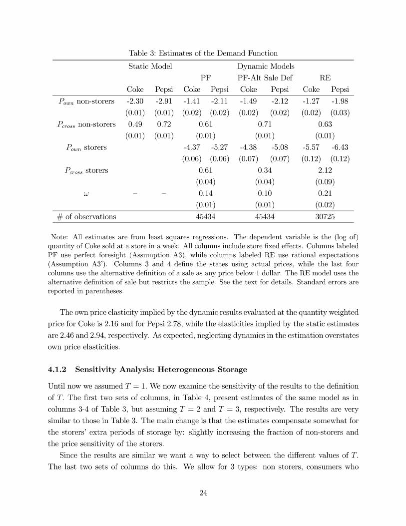
Table 3: Estimates of the Demand Function

Static Model Dynamic Models

PF PF-Alt Sale Def RE

Coke Pepsi Coke Pepsi Coke Pepsi Coke Pepsi

non-storers -2.30 -2.91 -1.41 -2.11 -1.49 -2.12 -1.27 -1.98

(0.01) (0.01) (0.02) (0.02) (0.02) (0.02) (0.02) (0.03)

non-storers 0.49 0.72 0.61 0.71 0.63

(0.01) (0.01) (0.01) (0.01) (0.01)

storers -4.37 -5.27 -4.38 -5.08 -5.57 -6.43

(0.06) (0.06) (0.07) (0.07) (0.12) (0.12)

storers 0.61 0.34 2.12

(0.04) (0.04) (0.09)

— — 0.14 0.10 0.21

(0.01) (0.01) (0.02)

# of observations 45434 45434 30725

Note: All estimates are from least squares regressions. The dependent variable is the (log of)

quantity of Coke sold at a store in a week. All columns include store fixed effects. Columns labeled

PF use perfect foresight (Assumption A3), while columns labeled RE use rational expectations

(Assumption A3’). Columns 3 and 4 define the states using actual prices, while the last four

columns use the alternative definition of a sale as any price below 1 dollar. The RE model uses the

alternative definition of sale but restricts the sample. See the text for details. Standard errors are

reported in parentheses.

The own price elasticity implied by the dynamic results evaluated at the quantity weighted

price for Coke is 2.16 and for Pepsi 2.78, while the elasticities implied by the static estimates

are 2.46 and 2.94, respectively. As expected, neglecting dynamics in the estimation overstates

own price elasticities.

4.1.2 Sensitivity Analysis: Heterogeneous Storage

Until now we assumed = 1We now examine the sensitivity of the results to the definition

of The first two sets of columns, in Table 4, present estimates of the same model as in

columns 3-4 of Table 3, but assuming = 2 and = 3, respectively. The results are very

similar to those in Table 3. The main change is that the estimates compensate somewhat for

the storers’ extra periods of storage by: slightly increasing the fraction of non-storers and

the price sensitivity of the storers.

Since the results are similar we want a way to select between the different values of

The last two sets of columns do this. We allow for 3 types: non storers, consumers who

24

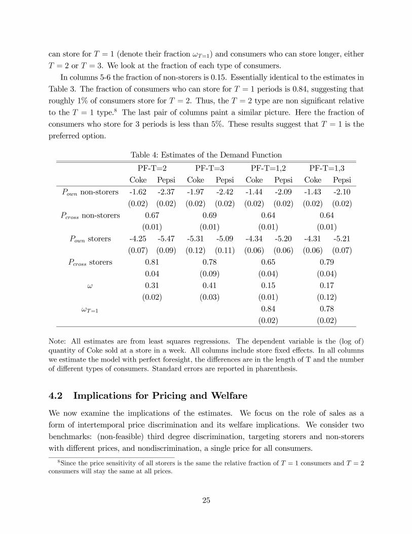
can store for = 1 (denote their fraction =1) and consumers who can store longer, either

= 2 or = 3. We look at the fraction of each type of consumers.

In columns 5-6 the fraction of non-storers is 0.15. Essentially identical to the estimates in

Table 3. The fraction of consumers who can store for = 1 periods is 0.84, suggesting that

roughly 1% of consumers store for = 2. Thus, the = 2 type are non significant relative

to the = 1 type.8 The last pair of columns paint a similar picture. Here the fraction of

consumers who store for 3 periods is less than 5%. These results suggest that = 1 is the

preferred option.

Table 4: Estimates of the Demand Function

PF-T=2 PF-T=3 PF-T=1,2 PF-T=1,3

Coke Pepsi Coke Pepsi Coke Pepsi Coke Pepsi

non-storers -1.62 -2.37 -1.97 -2.42 -1.44 -2.09 -1.43 -2.10

(0.02) (0.02) (0.02) (0.02) (0.02) (0.02) (0.02) (0.02)

non-storers 0.67 0.69 0.64 0.64

(0.01) (0.01) (0.01) (0.01)

storers -4.25 -5.47 -5.31 -5.09 -4.34 -5.20 -4.31 -5.21

(0.07) (0.09) (0.12) (0.11) (0.06) (0.06) (0.06) (0.07)

storers 0.81 0.78 0.65 0.79

0.04 (0.09) (0.04) (0.04)

0.31 0.41 0.15 0.17

(0.02) (0.03) (0.01) (0.12)

=1 0.84 0.78

(0.02) (0.02)

Note: All estimates are from least squares regressions. The dependent variable is the (log of)

quantity of Coke sold at a store in a week. All columns include store fixed effects. In all columns

we estimate the model with perfect foresight, the differences are in the length of T and the number

of different types of consumers. Standard errors are reported in pharenthesis.

4.2 Implications for Pricing and Welfare

We now examine the implications of the estimates. We focus on the role of sales as a

form of intertemporal price discrimination and its welfare implications. We consider two

benchmarks: (non-feasible) third degree discrimination, targeting storers and non-storers

with different prices, and nondiscrimination, a single price for all consumers.

8Since the price sensitivity of all storers is the same the relative fraction of = 1 consumers and = 2consumers will stay the same at all prices.

25

The analysis neglects the vertical relation between manufacturer and retailer, which could

generate double marginalization. The relation between retailers and manufacturers is quite

interesting and subtle, but beyond the scope of this paper. The first order conditions in

equation (10) represent either a manufacturer selling to a competitive retailing industry or

integrated pricing with transfers (which avoids double marginalization).

4.2.1 Markups and Profits

A standard exercise is to use demand estimates and a first order condition from a static

profit maximization to infer markups and marginal costs. Following this approach and using

the first two columns of Table 3 we get an implied markup for Coke of 43 cents, and 34 cents

for Pepsi. Subtracted from a quantity weighted average transaction price of 1.07 and 1.01,

respectively, leads to marginal costs of 66 and 67 cents respectively.

Repeating this calculation using the dynamic demand estimates reported in Table 3, but

still relying on a static first order condition, the implied margin for Coke is 50 cents and a

marginal costs of 57, while 37 and 64 cents for Pepsi. The lower dynamic elasticities translate

into higher implied mark-ups.

Naturally, demand dynamics render the static first order conditions inadequate as a de-

scription of seller behavior. So we now turn to the dynamic pricing model. We compute

prices and profits under non-discrimination, third degree discrimination and sales. We as-

sume the marginal cost during sale and non-sale periods is the same. Since each first order

condition delivers a different marginal cost, we use the average across the regimes to compute

prices and profits.

Table 5 displays the optimal regular, non-sale, prices and sale prices for Coke and Pepsi

under the different pricing assumptions. We also show profits relative to discrimination. By

discrimination we mean the case where the firms can identify the storers and non-storers,

set different prices for each group and prevent arbitrage. This is of course non-feasible but

serves as a benchmark to measure the maximum attainable gains from third degree price

discrimination.

By comparing the discriminatory and non-discriminatory prices we see the potential role

of sales in targeting price sensitive buyers with a lower price. The optimal non-discriminatory

price is 1.11 for Coke and 1.04 for Pepsi. These prices are in between the discriminatory

prices for both products: 1.31 and 0.83 for Coke and 1.14 and 0.86 for Pepsi. Non-storers,

being less price sensitive, are targeted with higher prices than storers. The discriminating

prices target non-storers with 58% higher Coke prices than storers’ prices. The gap is 33%

for Pepsi.

Rows labeled 3 and 4 present prices and profits under two different models of sales. The

numbers in row 3 use the demand estimates from columns 3-4 of Table 3 ( = 1 and perfect

26

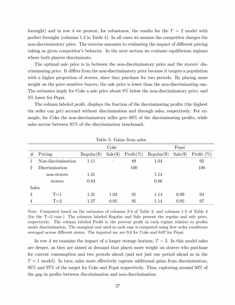
foresight) and in row 4 we present, for robustness, the results for the = 2 model with

perfect foresight (columns 1-2 in Table 4). In all cases we assume the competitor charges the

non-discriminatory price. The exercise amounts to evaluating the impact of different pricing

taking as given competitor’s behavior. In the next section we evaluate equilibrium regimes

where both players discriminate.

The optimal sale price is in between the non-discriminatory price and the storers’ dis-

criminating price. It differs from the non-discriminatory price because it targets a population

with a higher proportion of storers, since they purchase for two periods. By placing more

weight on the price sensitive buyers, the sale price is lower than the non-discriminating one.

The estimates imply for Coke a sale price about 8% below the non-discriminatory price, and

5% lower for Pepsi.

The column labeled profit, displays the fraction of the discriminating profits (the highest

the seller can get) accrued without discrimination and through sales, respectively. For ex-

ample, for Coke the non-discriminatory seller gets 88% of the discriminating profits, while

sales accrue between 91% of the discrimination benchmark.

Table 5: Gains from sales

Coke Pepsi

# Pricing Regular($) Sale($) Profit(%) Regular($) Sale($) Profit (%)

1 Non-discrimination 1.11 — 88 1.04 92

2 Discrimination 100 100

non-storers 1.31 1.14

storers 0.83 0.86

Sales

3 T=1 1.31 1.02 91 1.14 0.99 94

4 T=2 1.27 0.95 95 1.14 0.95 97

Note: Computed based on the estimates of columns 3-4 of Table 3, and columns 1-2 of Table 4

(for the T=2 case.) The columns labeled Regular and Sale present the regular and sale price,

respectively. The column labeled Profit is the percent profit in each regime relative to profits

under discrimination. The marginal cost used in each case is computed using first order conditions

averaged across different states. The imputed mc are 0.6 for Coke and 0.67 for Pepsi.

In row 4 we examine the impact of a longer storage horizon, = 2. In this model sales

are deeper, as they are aimed at demand that places more weight on storers who purchase

for current consumption and two periods ahead (and not just one period ahead as in the

= 1 model). In turn, sales more effectively capture additional gains from discrimination,

95% and 97% of the target for Coke and Pepsi respectively. Thus, capturing around 50% of

the gap in profits between discrimination and non-discrimination.

27

4.2.2 Welfare

The welfare consequences of third degree price discrimination had been studied since Robin-

son (1933). The standard intuition is that in a monopoly situation price discrimination

will yield lower prices in the weak market, where the demand is more price sensitive, and

higher prices in the strong market, relative to the non-discriminatory price.9 So while sell-

ers are better off, some consumers are better off and others worse off. The overall impact

of discrimination is an open question subsequently studied by Schmalensee (1981), Varian

(1984), Aguirre, Cowan and Vickers (2010) among others. A necessary condition for welfare

to improve is that quantity sold increases. Since the allocation of goods across markets is

distorted, a constant —or lower— output would necessarily lead to lower total surplus (for a

formal proof see Schmalensee (1981)).

In the context of a duopoly the picture is slightly more complex, as it is not even clear

sellers are better off under discrimination. Few papers provide theoretical results. Boren-

stein (1985) and Holmes (1989) offer conditions for output to increase under duopoly, and

simulations showing profits may decline. Corts (1998) shows that even with well behaved

profit functions all prices can decrease when the weak market of one firm is the strong market

of the other.

In this section we evaluate the impact of intertemporal discrimination on quantity and

welfare. We first consider the implication of our estimates for a monopolist (i.e., a duopolist

that unilaterally best responds to given competitor behavior), and compare the findings to

the theoretical literature. We then consider the duopoly case where there is little theoretical

guidance.

Best Responses As a first step we compute quantity changes holding fixed the behavior

of competitors and assuming these competitors do not price discriminate. This allows us to

isolate the impact of different pricing strategies. An additional advantage of this exercise is

that it is linked to the theoretical results in Schmalensee (1981) and Aguirre et. al. (2010),

since the seller is basically a monopolist.

It is worth mentioning that the third-degree discrimination theoretical results apply to

the intertemporal price discrimination as well. We just need to reinterpret demand during

sale periods, () + 2(), as the weak demand, and demand during non-sale periods,

() as the strong demand.

Before looking at the numbers in Table 6 we turn to the theoretical literature for pre-

dictions and to make sure the functional forms we use are not responsible for our findings.

9The direction of price changes indeed follows this pattern if the monopolist’s profit function is strictly

concave in price within each segment. When this is not the case the direction of price changes is ambiguous

(see Nahata, et al. (1990))

28

Proposition 3 in Aguirre et al. (2010) encompasses our demand framework. They show that

welfare depends on the relative concavity of the demand functions in the two markets. Our

estimates deliver a more convex demand in the weak market, which is one of the conditions

singled out in Robinson (1933) for quantity to increase under discrimination. In addition,

what Aguirre et al. call the IRC condition10 holds for exponential demands, thus Proposition

3 therein applies. Proposition 3 is a comparative static with respect to the degree of price

discrimination.11 Proposition 3 shows that, for our estimated demand, welfare increases in

the extent of discrimination and then declines. A little discrimination is welfare improving,

full discrimination could deliver higher or lower welfare. In sum, even in the monopoly case

the impact on welfare is indeterminate. It is an empirical matter that we will evaluate with

the estimates.

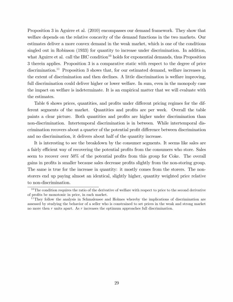
Table 6 shows prices, quantities, and profits under different pricing regimes for the dif-

ferent segments of the market. Quantities and profits are per week. Overall the table

paints a clear picture. Both quantities and profits are higher under discrimination than

non-discrimination. Intertemporal discrimination is in between. While intertemporal dis-

crimination recovers about a quarter of the potential profit difference between discrimination

and no discrimination, it delivers about half of the quantity increase.

It is interesting to see the breakdown by the consumer segments. It seems like sales are

a fairly efficient way of recovering the potential profits from the consumers who store. Sales

seem to recover over 50% of the potential profits from this group for Coke. The overall

gains in profits is smaller because sales decrease profits slightly from the non-storing group.

The same is true for the increase in quantity: it mostly comes from the storers. The non-

storers end up paying almost an identical, slightly higher, quantity weighted price relative

to non-discrimination.

10The condition requires the ratio of the derivative of welfare with respect to price to the second derivative

of profits be monotonic in price, in each market.11They follow the analysis in Schmalensee and Holmes whereby the implications of discrimination are

assessed by studying the behavior of a seller who is constrained to set prices in the weak and strong market

no more then units apart. As increases the optimum approaches full discrimination.

29

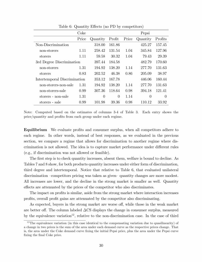
Table 6: Quantity Effects (no PD by competitors)

Coke Pepsi

Price Quantity Profit Price Quantity Profits

Non-Discrimination 318.00 161.86 425.27 157.45

non-storers 1.11 258.42 131.54 1.04 345.84 127.96

storers 1.11 59.58 30.32 1.04 79.43 29.39

3rd Degree Discrimination 397.44 184.58 482.79 170.60

non-storers 1.31 194.92 138.20 1.14 277.70 131.63

storers 0.83 202.52 46.38 0.86 205.09 38.97

Intertemporal Discrimination 353.12 167.78 446.06 160.44

non-storers-non-sale 1.31 194.92 138.20 1.14 277.70 131.63

non-storers-sale 0.99 307.36 118.64 0.98 394.18 121.41

storers - non-sale 1.31 0 0 1.14 0 0

storers - sale 0.99 101.98 39.36 0.98 110.12 33.92

Note: Computed based on the estimates of columns 3-4 of Table 3. Each entry shows the

price/quantity and profits from each group under each regime.

Equilibrium We evaluate profits and consumer surplus, when all competitors adhere to

each regime. In other words, instead of best responses, as we evaluated in the previous

section, we compare a regime that allows for discrimination to another regime where dis-

crimination is not allowed. The idea is to capture market performance under different rules

(e.g., if discrimination was not allowed or feasible).

The first step is to check quantity increases, absent them, welfare is bound to decline. As

Tables 7 and 8 show, for both products quantity increases under either form of discrimination,

third degree and intertemporal. Notice that relative to Table 6, that evaluated unilateral

discrimination —competitors pricing was taken as given— quantity changes are more modest.

All increases are lower, and the decline in the strong market is smaller as well. Quantity

effects are attenuated by the prices of the competitor who also discriminates.

The impact on profits is similar, aside from the strong market where interaction increases

profits, overall profit gains are attenuated by the competitor also discriminating.

As expected, buyers in the strong market are worse off, while those in the weak market

are better off. The column labeled ∆CS displays the change in consumer surplus, measured

by the equivalence variation12, relative to the non-discrimination case. In the case of third

12The equivalence variation (in this case identical to the compensating variation due to quasilinearity) of

a change in two prices is the sum of the area under each demand curve as the respective prices change. That

is, the area under the Coke demand curve fixing the initial Pepsi price, plus the area under the Pepsi curve

fixing the final Coke price.

30

degree discrimination non-stores are worse off but storers are better off because they are

offered lower prices. In the case of intertemporal discrimination, non-storers can partly

benefit from the sales but are charged higher prices during non-sale periods; overall they are

worse off. Storers are better off in both cases, but less so under intertemporal discrimination

because the prices they are charged are not as low as under third degree discrimination.

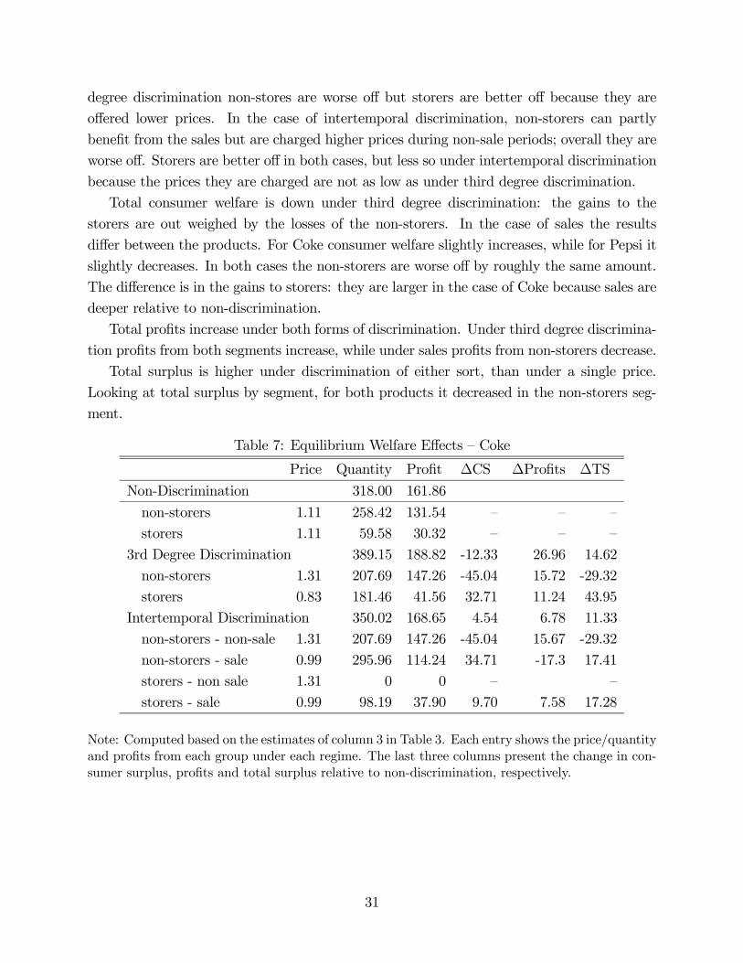
Total consumer welfare is down under third degree discrimination: the gains to the

storers are out weighed by the losses of the non-storers. In the case of sales the results

differ between the products. For Coke consumer welfare slightly increases, while for Pepsi it

slightly decreases. In both cases the non-storers are worse off by roughly the same amount.

The difference is in the gains to storers: they are larger in the case of Coke because sales are

deeper relative to non-discrimination.

Total profits increase under both forms of discrimination. Under third degree discrimina-

tion profits from both segments increase, while under sales profits from non-storers decrease.

Total surplus is higher under discrimination of either sort, than under a single price.

Looking at total surplus by segment, for both products it decreased in the non-storers seg-

ment.

Table 7: Equilibrium Welfare Effects — Coke

Price Quantity Profit ∆CS ∆Profits ∆TS

Non-Discrimination 318.00 161.86

non-storers 1.11 258.42 131.54 — — —

storers 1.11 59.58 30.32 — — —

3rd Degree Discrimination 389.15 188.82 -12.33 26.96 14.62

non-storers 1.31 207.69 147.26 -45.04 15.72 -29.32

storers 0.83 181.46 41.56 32.71 11.24 43.95

Intertemporal Discrimination 350.02 168.65 4.54 6.78 11.33

non-storers - non-sale 1.31 207.69 147.26 -45.04 15.67 -29.32

non-storers - sale 0.99 295.96 114.24 34.71 -17.3 17.41

storers - non sale 1.31 0 0 — —

storers - sale 0.99 98.19 37.90 9.70 7.58 17.28

Note: Computed based on the estimates of column 3 in Table 3. Each entry shows the price/quantity

and profits from each group under each regime. The last three columns present the change in con-

sumer surplus, profits and total surplus relative to non-discrimination, respectively.

31

Table 8: Equilibrium Welfare Effects — Pepsi

Price Quantity Profit ∆CS ∆Profits ∆TS

Non-Discrimination 425.27 157.35

non-storers 1.04 345.84 127.96 — — —

storers 1.04 79.43 29.39 — — —

3rd Degree Discrimination 486.62 181.56 -16.38 24.21 7.83

non-storers 1.14 313.73 148.71 -36.49 20.75 -15.74

storers 0.86 172.89 32.85 20.10 3.46 23.56

Intertemporal Discrimination 441.87 162.14 -2.22 4.79 2.57

non-storers - non-sale 1.14 313.73 148.71 -36.49 20.75 -15.74

non-storers - sale 0.98 365.68 112.63 21.25 -15.33 5.92

storers - non sale 1.14 0 0 — — —

storers - sale 0.98 102.16 31.47 5.40 2.08 7.48

Note: Computed based on the estimates of column 4 in Table 3. Each entry shows the price/quantity

and profits from each group under each regime. The last three columns present the change in con-

sumer surplus, profits and total surplus relative to non-discrimination, respectively.

5 Concluding Comments

We study the impact of price discrimination when consumers can anticipate demand and

store for future consumption. To make the problem tractable we offer a simple model to

account for demand dynamics due to consumer inventory behavior. We estimate the model

using store level scanner data and find that consumers who store are more price sensitive.

This suggests that intertemporal price discrimination can potentially increase profits, which

we then quantify. We find that sales can recover 24-30% of the potential gains from (non-

feasible) third degree price discrimination. The estimates also suggest that total welfare

increases when sales are offered.

A key to making our model tractable is the simplicity, some might say over-simplicity, of

the demand model. Its important to note that in order to take the general demand model in

Section 2.1 to the data one needs to also make some strong (mostly untestable) assumptions

regarding, for example, the functional form of inventory cost and consumer expectations

on how prices evolve (see, for example, Erdem, Imai and Keane, 2003, or Hendel and Nevo,

2006b). It depends on the application whether it is more reasonable to make the assumptions

of this paper or those of the previous literature. If one is willing to make the assumptions

herein the analysis is significantly simpler and in many issues, like the supply side, becomes

tractable.

32

6 References

Aguirre, Inaki, Simon Cowan and John Vickers (2010) "Monopoly Price Discrimination and

Demand Curvature" American Economic Review, Volume 100, Number 4, September,

pp. 1601-1615(15)

Berry, Steven, James Levinsohn, and A. Pakes (1995), “Automobile Prices in Market Equi-

librium,” Econometrica, 63, 841-890.

Blattberg, R. and S. Neslin (1990), Sales Promotions, Prentice Hall.

Boizot, C., J.-M. Robin, M. Visser (2001), “The Demand for Food Products. An Analysis of

Interpurchase Times and Purchased Quantities,” Economic Journal, 111(470), April,

391-419.

Borenstein, Severin (1985). "Price Discrimination in Free-Entry Markets" The RAND

Journal of Economics, Vol. 16, No. 3 (Autumn, 1985), pp. 380-397.

Chevalier, Judith and Anil Kashyap. (2010) "Best Prices" mimeo University of Chicago.

Conlisk J., E. Gerstner, and J. Sobel “Cyclic Pricing by a Durable Goods Monopolist,”

Quarterly Journal of Economics, 1984.

Corts, Kenneth. (1998) "Third-Degree Price Discrimination in Oligopoly: All-Out Com-

petition and Strategic Commitment", The RAND Journal of Economics, Vol. 29, No.

2, pp. 306-323.

Erdem, T., M. Keane and S. Imai (2003), “Consumer Price and Promotion Expectations:

Capturing Consumer Brand and Quantity Choice Dynamics under Price Uncertainty,”

Quantitative Marketing and Economics, 1, 5-64.

Hendel, Igal and Aviv Nevo “Sales and Consumer Inventory,” Manuscript, Rand Journal

of Economics, 2006a.

Hendel, Igal and Aviv Nevo “Measuring the Implications of Sales and Consumer Inventory

Behavior,” Econometrica, 2006b.

Holmes, Thomas (1989) "The Effect of Third Degree Price Discrimination in Oligopoly"

American Economic Review, Vol. 79, No. 1, March, pp. 244-250

Hong P., P. McAfee, and A. Nayyar “Equilibrium Price Dispersion with Consumer Inven-

tories”, Journal of Economic Theory, Vol 105, Issue 2, Pages 503-517.

33

Jeuland, Abel P. and Chakravarthi Narasimhan. “Dealing-Temporary Price Cuts-By Seller

as a Buyer Discrimination Mechanism” Journal of Business, Vol. 58, No. 3. (Jul.,

1985), pp. 295-308.

Nahata, B., Ostaszewski, K. and Sahoo, P.K. “Direction of Price Changes in Third-Degree

Price Discrimination.” American Economic Review, Vol. 80 (1990), pp. 1254-1258.

Perrone, Helena (2010). "Inventories, Unobservable Heterogeneity, and Long-Run Elastici-

ties" mimeo Pompeu Fabra.

Pesendorfer, Martin (2002), “Retail Sales. A Study of Pricing Behavior in Supermar-

kets,”Journal of Business, 75(1), 33-66.

Robinson, Joan (1933), "The Economics of Imperfect Competition" McMillan and Co.

Salop S. and J. E. Stiglitz. (1982) “The Theory of Sales: A Simple Model of Equilibrium

Price Dispersion with Identical Agents” The American Economic Review, Vol. 72, No.

5, Dec., pp. 1121-1130.

Schmalensee, Richard (1981) "Output and Welfare Implications of Monopolistic Third-

Degree Price Discrimination" American Economic Review, Vol. 71, No. 1 (March),

pp. 242-247.

Shepard, Andrea. (1991) "Price Discrimination and Retail Configuration," The Journal of

Political Economy, Vol. 99, No. 1, Feb., pp. 30-53

Sobel, Joel. “The Timing of Sales,” Review of Economic Studies, 1984.

Varian, Hal “A Model of Sales” The American Economic Review, Vol. 70, No. 4. (Sep.,

1980), pp. 651-659.

Varian, Hal (1985) "Price Discrimination and Social Welfare" American Economic Review,

Vol. 75, No. 4 September, pp. 870-875.

Verboven, Frank.(1996) "International Price Discrimination in the European Car Market,"

The RAND Journal of Economics, Vol. 27, pp. 240-268

Villas Boas, S. (2009) "An empirical investigation of the welfare effects of banning wholesale

price discrimination," The Rand Journal of Economics, Vol. 40, pp 20-46.

34

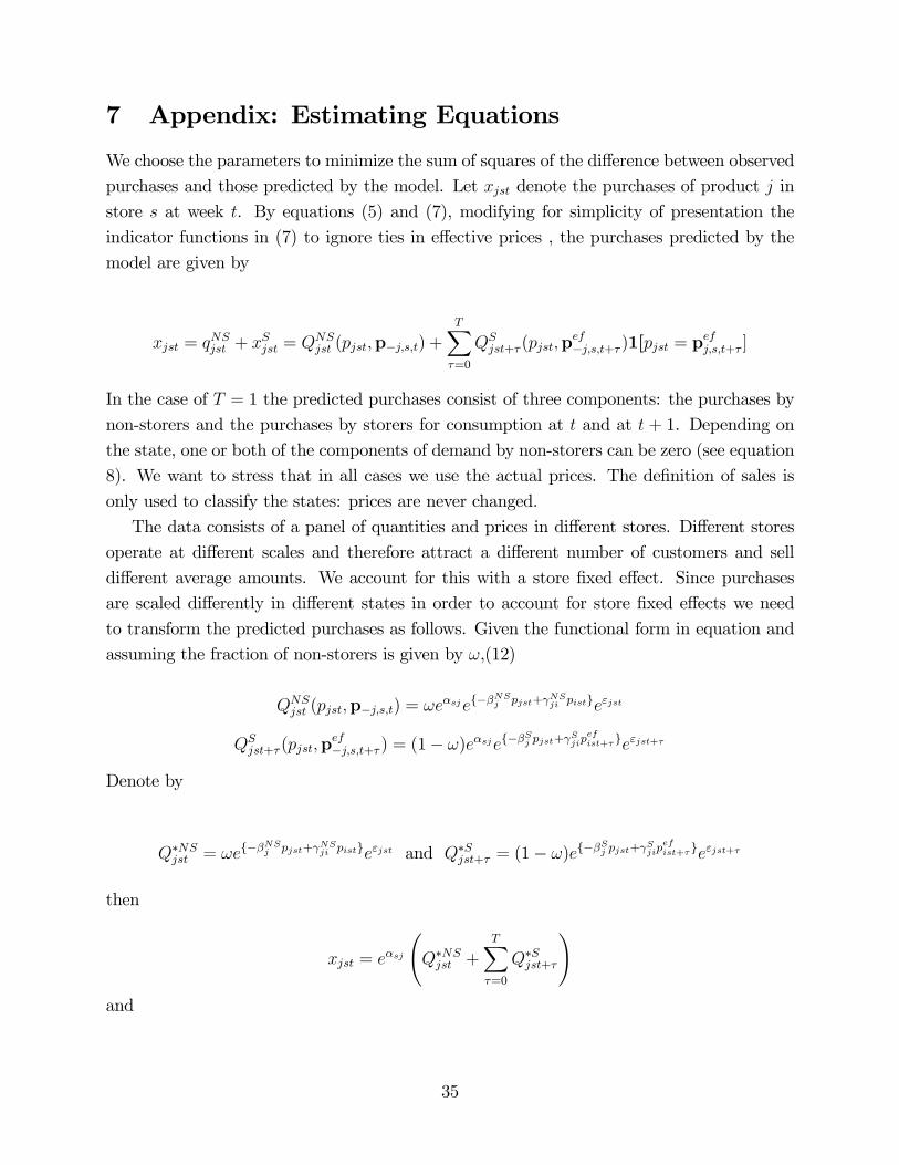
7 Appendix: Estimating Equations

We choose the parameters to minimize the sum of squares of the difference between observed

purchases and those predicted by the model. Let denote the purchases of product in

store at week . By equations (5) and (7), modifying for simplicity of presentation the

indicator functions in (7) to ignore ties in effective prices , the purchases predicted by the

model are given by

= + =

(p−) +X

=0

+(p

−+)1[ = p

+ ]

In the case of = 1 the predicted purchases consist of three components: the purchases by

non-storers and the purchases by storers for consumption at and at + 1. Depending on

the state, one or both of the components of demand by non-storers can be zero (see equation

8). We want to stress that in all cases we use the actual prices. The definition of sales is

only used to classify the states: prices are never changed.

The data consists of a panel of quantities and prices in different stores. Different stores

operate at different scales and therefore attract a different number of customers and sell

different average amounts. We account for this with a store fixed effect. Since purchases

are scaled differently in different states in order to account for store fixed effects we need

to transform the predicted purchases as follows. Given the functional form in equation and

assuming the fraction of non-storers is given by ,(12)

(p−) = {−

+

}

+ (p

−+) = (1− ){−

+

+}+

Denote by

∗ = {−

+

} and ∗+ = (1− ){−

+

+}+

then

=

Ã∗

+X

=0

∗+

!and

35

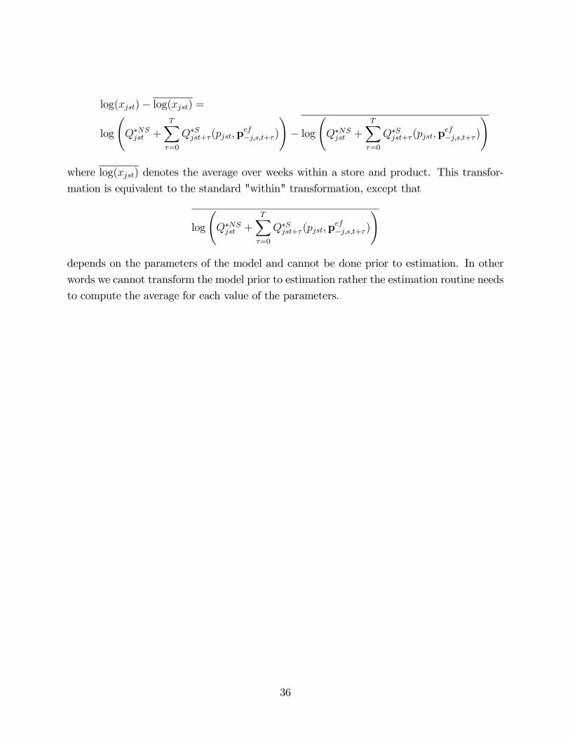
log()− log() =

log

Ã∗ +

X=0

∗+(p−+ )

!− log

Ã∗ +

X=0

∗+(p−+)

!

where log() denotes the average over weeks within a store and product. This transfor-

mation is equivalent to the standard "within" transformation, except that

log

Ã∗ +

X=0

∗+(p−+ )

!

depends on the parameters of the model and cannot be done prior to estimation. In other

words we cannot transform the model prior to estimation rather the estimation routine needs

to compute the average for each value of the parameters.

36