Intertemporal Price Discrimination and Investment in Brand Equity

Sudha KrishnaswamiDepartment of Finance

College of Business AdministrationUniversity of New OrleansNew Orleans, LA 70148

(504) 280-6488email: skrishn1@uno.edu

Sri B. RaghavanSenior Consultant

i2 Technologies, Inc.909 E. Los Colinas Blvd.

Irving, TX 75039(973) 495-6304

Venkat Subramaniam*

A. B. Freeman School of BusinessTulane University

New Orleans, LA 70118(504) 865-5493

email: vencat@tulane.edu

______________________________

* Corresponding author. We thank Victor Cook, J. Ronnie Davis, Mark Johnson, Srini Krishnamurthy, HaimMano, Bill Mead, Tom Noe, Bill Ross, Paul Speck, and the seminar participants at the University of Missouri–St.Louis, University of New Orleans, and the INFORMS Marketing Science conference at Berkeley for their valuablecomments and suggestions.

Intertemporal Price Discrimination and Investment in Brand Equity

Abstract

We consider a firm that produces a specialty or a branded image good, where consumersderive part of their utility from the eliteness of the brand’s image and exclusivity of the product.Once high valuation consumers have purchased the product, it is optimal for the firm to reduce theprice and capture lower valuation consumers. However, this dilutes the exclusivity of the brand,and results in a perceived loss to the high valuation consumers. In a two-period model, we showthat if a firm is unable to credibly commit to not lowering the price in the second period, the firstperiod price is adversely affected. We demonstrate that through a positive investment in brandequity that promotes the eliteness of the brand’s image, the firm can enhance the first periodconsumers’ utility from owning the product and thus offset their perceived loss in the secondperiod. This higher utility encourages more consumers to buy the product in the first period, andmitigates the firm’s losses when the firm is unable to commit to a price path. More importantly,we show that an investment in brand equity is unlike an investment that enhances a tangible aspectof a product, in that, it substitutes for a firm’s ability to commit to a non-discriminatory price path.We establish this result by demonstrating that although a positive level of investment in brandequity is optimal irrespective of a firm’s ability to commit to a price path, the benefits from theinvestment are higher when the firm is unable to commit than when it is able to commit to a pricepath.

JEL Classification: D91, D92, L11

1

“I went into the Versace Store on Madison Avenue and tried on a raspberry suit. It was $1400. Idecided to think about it. I then went into a (factory direct) store and saw it on sale for $299. Mysnobbery is not worth the $1,101 difference. This may not be loyal to the antiquated standards ofbusiness, but it’s very local to a customer’s intelligence.”

- Peter Glen, Author, Speaker, and Sales Promotion Consultant.1

In the summer of 1995, BMW started offering a new $20,000 version of its popular 3-

Series cars, the 318ti. This car was priced significantly below BMW’s previous entry-level

models. While the intent of the automaker was to expand its reach to younger, less affluent

buyers, critics felt that BMW ran the risk of turning off prestige conscious buyers.2 Similar

moves to downscale the market using the original brand name is also true of other big brand names

such as Giorgio Armani that introduced the Giorgio Armani General store and the Armani

Exchange. Further evidence of the above phenomenon may be seen in the recent growth in outlet

malls that provide discounted merchandise of brand names such as Gucci, Calvin Klein, Liz

Claiborne and Polo by Ralph Lauren.

From the consumers’ point of view, an important problem arises when a firm attempts to

lower its price and appeal to a downscale market. When an upscale brand name is sold at a

premium in one period and is then discounted during the second period, more consumers purchase

the product. That is, more consumers enter into an elite group to which the first period consumers

belong. Thus, there is a perceived loss of value to the first period consumers that stems from the

dilution in the degree of uniqueness or exclusivity of the brand name. Of course, consumers’

anticipation of this loss may result either in a lower demand or in a lower price for the firm’s

products in the first period.3 It should be noted that even though the move downscale may on

1 See the “Two Magic Words for Retailing Success,” Direct Marketing, October 1991, p. 46 - 47.2 See “BMW’s $20,000 318ti,” Ward’s Auto World, August 1995, p. 50.3 Indirect evidence of the above problem may be seen from the fact that manufacturers of prestige brand names (suchas the shoe maker G.H.Bass & Co., Gant sportswear, and Van Heusen) and retailers (such as Nordstrom, and SaksFifth Avenue) who have a presence in outlet malls do not allow their names to be used in print, television, or radioads for the outlet malls. Most are reluctant to even discuss these operations publicly. Thus, when upscalemanufacturers price discriminate, they primarily depend on word of mouth, and when broader promotions are required,they restrict themselves to billboards and publications that target only factory outlet shoppers. (See Barron’s, March21, 1994, p. 52-53, and Business Week, February 3, 1986, p. 92-93).

2

some occasions involve products with fewer features, as long as it is under the same brand name,

the perceived loss due to the dilution of brand exclusivity still exists for the first period consumers.

In this paper, we consider a firm that produces an image good where the firm decides to

lower its price after one period to attract a downscale market. The exclusivity of the brand is

diluted as more consumers purchase the product in the second period. In a two-period framework,

we model the consumers’ rational anticipation of the firm’s incentive to price discriminate and the

impact of such anticipation on the price of the product in the first period. We show that when a

firm is unable to commit to not lowering the price in the second period, the price in the first period

is adversely affected.

We argue that a part of the value derived by consumers from an image good may be viewed

as a function of both the number of other consumers who own the product (exclusivity of the

brand) and the level of investment in brand equity made by the firm to promote the eliteness of the

brand’s image. In this context, we define brand equity as the incremental value endowed by the

brand to the product (Furquhar, 1989). Thus, investment in brand equity includes expenditure on

advertisements that target an upscale clientele, investment incurred in positioning the product in

prestigious retail outlets, and investments in other promotions that enhance the image and

distinction associated with owning the product. In this scenario, an investment in brand equity

coupled with the exclusivity of the product in the first period enhances consumers’ utility from

owning the product in the first period. We argue that this higher utility encourages more

consumers to buy the product in the first period than wait for the lower second period price. Thus,

an investment in brand equity in the first period helps the firm mitigate the adverse effect on a

product’s first period price when the firm is unable to commit to a non-discriminatory price path.

An investment in brand equity is unlike an investment that enhances a tangible aspect of a

product, in that, it substitutes for a firm’s ability to commit to a non-discriminatory price path. We

establish this result by demonstrating that although a positive level of investment in brand equity is

optimal in the first period irrespective of a firm’s ability to commit to a price path, the benefit from

the investment is higher when the firm is unable to commit than when it is able to commit to a non-

3

discriminatory price path. Finally, we show that indiscriminate investment in brand equity is sub-

optimal. The optimal investment is dictated by the rate at which consumers’ utility from the image

and eliteness of owning the product in the first period increases with additional investment in brand

equity.

Our paper is closely related to the literature on intertemporal price discrimination. In a

seminal paper, Coase (1972) argues that in a multi-period model, durability fully eliminates a

monopolist’s market power if the length of time between price adjustments tends to zero. The

intuition behind his argument is that if consumers anticipate that the price will be lowered in the

next instant, their cost to waiting to buy is negligible and hence, they cannot be induced to pay a

price above the competitive price. This conjecture is formally established by Stokey (1981) and

Bulow (1982) for specific demand functions.4 Besanko and Winston (1990) study the

intertemporal pricing policy of a firm in a discrete-time, finite horizon model, where consumers are

rational and their valuations of the product are distributed uniformly. They derive the subgame

perfect pricing policy and show that when the discount factor is less than one, the optimal price

path involves intertemporal price discrimination. In a similar vein, Moorthy and Png (1992)

consider the problem of product cannibalization when a monopolist introduces two differentiated

products simultaneously. They show that in this context, a sequential introduction of the high

quality product followed by the lower quality product is optimal when consumers are more

impatient than the monopolist, i.e., when their discount factor is lower than that of the

monopolist.5

In this paper, we show that through an investment in brand equity that promotes the

eliteness of the brand’s image, a firm will be able to price discriminate more efficiently. An

implication of our paper is that even when discount factors are identical across investors (i.e.,

4 Stokey (1979) shows that for some class of consumer utility functions, the Coase conjecture obtains even whentime between price adjustments is not small.5 Levinthal and Purohit (1989) also consider the problem of a firm’s old product cannibalizing the firm’s newproduct, and show that when modest levels of product improvements are made, phasing out the old product issuperior to a policy of either buying back the old product or announcing the introduction of the new product.

4

capital markets are perfect), or when the discount factors of the consumers and the firm are

exogenous, higher valuation consumers may be made more “impatient” through higher investment

in brand equity. Further, there is an important difference between investment in brand equity and

the standard discount factor, in that, in the former, investment is not only a choice variable but it is

also a mechanism where the cost is incurred only by the firm and not by the consumer. Therefore,

by establishing the optimality of a positive investment in brand equity we demonstrate that price

discrimination is beneficial to the firm even if it can only be achieved at a cost.

Our paper is also related to the work of Bulow (1986) and Waldman (1996) who show that

firms may not be able to price discriminate efficiently when there is a perfect second-hand market.

This is because the firm’s first period products act as substitutes for the firm’s products in the

second period. In this scenario, Bulow shows that it is optimal for the firm to produce goods that

have uneconomically short useful lives. This planned obsolescence is optimal because competition

in the subsequent periods will be between related, but not identical, substitute products. Waldman

interprets durability as the rate at which the product’s quality deteriorates, and shows that the firm

selects a durability choice that is below the first best level. Since the price of the new units are

limited by the price of the old units in the secondhand market, reducing durability enables the firm

to set a higher price for the new units. The results of our model imply that even if durability is

fixed and cannot be shortened, the firm can still price discriminate since its investment in brand

equity induces more of the high valuation consumers to buy the product in the first period.

The rest of the paper is organized as follows. In Section II we describe the model and the

underlying assumptions. We also illustrate the effect of the consumers’ perceived loss problem on

the first period price of the product, and on the firm’s profits. In Section III we consider a firm

that is unable to credibly commit to a future price path, and show that a positive investment in

brand equity is optimal to the firm. In Section IV we show that even for a firm that is able to

commit to a non-discriminatory price path, investment in brand equity is optimal. However, this

optimal level of investment is lower than that of a firm which is unable to commit to abstaining

from price discrimination. Thus, investment in brand equity provides additional value for a firm

5

that is unable to commit to a non-discriminatory price path compared to a firm that is able to

commit. Section V presents concluding comments.

II. Model and Assumptions

Consider a monopolist firm that faces a downward sloping demand function for its

product. Let the consumption demand for the product be p = 1 - q, where p is the market clearing

price of the product and q is the total output produced by the firm. Also, let the consumers’

valuation of the product be uniformly distributed on the closed interval [0,1]. Consider a 3-date 2-

period model, in which the firm first decides on its level of investment in brand equity on date 0,

and then initiates production subsequent to this investment stage. Production is completed and the

output is revealed to the market on date 1.

In this paper, we define the date 0 investment in brand equity as one that is made by the

firm to promote the eliteness of the brand’s image. As in Furquhar (1989) we view the brand

equity of a firm as the incremental value endowed by the brand to the product. The incremental

value typically stems from investments made by the firm on date 0 to enhance the brand’s

perceived quality and other positive brand associations besides quality. This characterization of

brand equity captures the value received by consumers that is in addition to the pure service value

of the product. An example of such non-service value is in Aaker (1991) who notes that “knowing

that a piece of jewelry came from Tiffany can affect the experience of wearing it; the user can

actually feel differently because of Tiffany’s perceived quality and associations.” Thus, investment

in brand equity includes expenditure on advertisements that target an upscale clientele. It also

includes investment in positioning the product in prestigious retail outlets and in other promotions

that enhance the image and distinction associated with owning the product. In the empirical

taxonomy of the impact of advertising expenditure on quality as specified in Moorthy and Zhao

(1996), this investment should be viewed as one that enhances the intangible attributes such as

perceived quality, as opposed to the one that increases the objective quality of the product.

The firm also has the option of producing more output over the second period and selling

this output on date 2. We assume that over the two periods consumers buy the product at most

6

once. For simplicity, we also assume that date 1 consumers do not resell their products on date 2.

This formulation allows us to focus on the effect of brand equity on pricing policy without the

confounding effects of second hand markets, and is also in the tradition of the existing literature

(Besanko and Winston, 1990; and Moorthy and Png, 1992). Thus, the date 2 consumption

demand for the product is p = 1 - q1 - q, where q1 is the output sold on date 1. Also, irrespective

of whether the product was purchased on date 1 or date 2, once a consumer buys and initiates the

use of the product it lasts for a finite period of time, say, N (≥ 2) periods. Therefore, when we

consider only the direct service offered by the product, the service value derived by the consumers

who purchase the product on date 1 is identical to that derived by the consumers who purchase the

product on date 2. We refer to the consumers who buy the product first (i.e., on date 1) as high

valuation consumers and those that buy the product on date 2 as low valuation consumers.

We assume perfect capital markets where the interest rate is determined by exogenous,

economy-wide factors. We also assume that all agents maximize expected discounted present

value. In this context, since the interest rate is just a scaling factor, we assume it to be zero. We

denote the firm’s date 1 and date 2 operating profits (revenues minus production costs) by Π1 and

Π2 respectively. For simplicity, we also assume that the marginal cost of production is constant,

and without loss of generality set it to zero. We assume that the product is a specialty or branded

image good. In other words, in our model, consumers receive two types of value from the product

-- (i) the pure service value of the product, and (ii) the value from the eliteness of the brand’s image

and the exclusivity of owning the product. This latter brand value is not only a function of the

brand equity investment made by the firm to promote the eliteness of the brand, but also implicitly

an inverse function of the number of other consumers who own the product. Therefore, this

component of value disappears in the second period when the exclusivity of the brand is diluted.6

This implicitly assumes that investment in brand equity towards promoting non-exclusive goods

6 Alternatively, we may assume that the value from the brand image diminishes (instead of disappears) withadditional consumers. Following proposition 2 we discuss the implications of such a formulation and argue that it

7

(generic products) would not add any value to the consumers. This assumption characterizes the

nature of the products discussed as examples in the previous section, in that, when a firm that

produces an image good lowers the price on date 2, consumers who bought the product on date 1

would perceive a value loss. This loss is a consequence of the firm downscaling its market

(expanding to low valuation consumers), thereby diluting the exclusivity of the product that was

sold to the first period consumers.

Below, we first establish formally that once the high valuation consumers have purchased

the product on date 1, the firm has the incentive to cut the price of the product on date 2. This

results in the perceived loss to the first period consumer. Since the pure service value derived from

the product bought on date 1 is identical to that from the new product bought on date 2, the

difference between the product’s price in the two periods represents the first period consumers’

loss from dilution of the brand’s image and exclusivity.

Lemma 1: If the firm sets the standard monopoly output on date 1, and if the consumers whose

valuation exceed the corresponding monopoly price buy the product on date 1, then these

consumers lose a value of L = 1/4, when the firm sells more output on date 2.

Proof: The optimal monopoly output q1* on date 1 is:

argmaxq 1

q1 (1-q1) where, q1 is the date 1 output of the firm.

This implies that q1* = 1/2 and the corresponding date 1 price of the product is p1

* = 1/2.

Once consumers whose valuations exceed 1/2 buy the product on date 1, consider the firm’s

incentives on date 2. On date 2, the firm faces a residual demand function of p = (1 - q1* ) - q, i.e.,

p = 1/2 - q. The optimal strategy for the firm on date 2 is to therefore set an output q2* , where

q2* is argmax

q 2

q2 (1/2-q 2 ).

So, q2* = 1/4 and p2

* = 1/4.

Hence the perceived loss to the consumers who bought the product on date 1 is

does not alter our main results.

8

p1* - p2

* = 1/ 4 . ♦

The result that the first period consumers lose when the firm price discriminates in the

second period assumes that the consumers are myopic, that is, they do not rationally anticipate the

firm’s incentive to lower the price in the second period. However, if we assume rational agents,

then the second period incentives of all participants are correctly anticipated by all the other

participants. In this scenario, since the date 1 consumers anticipate the lowering of the price on

date 2 they do not pay the standard consumption demand price for the product on date 1. Instead,

the equilibrium market price would be the lower of either the consumption demand price or the

expected second period price. For a given first period output of q1 , the corresponding

consumption demand price is (1-q1 ), and the firm then faces a residual demand of p = (1-q1 )-q in

the second period. Therefore, the optimal second period output is (1-q1 )/2, the corresponding

price is (1-q1 )/2, and so the first period consumers will perceive a loss of [(1-q1 ) - (1- q1 )/2].

This loss is zero only when q1 = 1, that is, only when the first period price is equal to zero.

Hence, when the consumers are rational and the firm is unable to commit not to price discriminate,

the market fails to clear at any price p > 0.7 In our two-period model though, the firm has another

option. It could set a zero output on date 1 and confine all production and sale of output to only

date 2. Here the firm is able to avoid the adverse consequence of its inability to commit not to price

discriminate, since by assumption, there is no production subsequent to date 2. This scenario is

equivalent to a one period model, and the firm then sets an output q* = 1/2 (and the corresponding

price p* = 1/2), and receives a profit of 1/4.

Our result that no output is sold in the first period differs from the one in Tirole (1990, p.

81-82). This is because of a fundamental difference between our two models. In a two period

framework, Tirole assumes that the second period consumers use the product for one period less

7 Had we assumed an interest rate greater than zero (i.e., discount factor < 1), consumers with very high valuationwill buy the product on date 1 due to the increased time value of utility from a date 1 purchase. In the next section,we show that even if the discount factor is equal to 1, high valuation consumers may be made impatient (i.e., will

9

than the first period consumers. On the other hand, in our model production takes place again in

the second period, and a new product lasts the same length of time irrespective of whether it was

produced in the first or the second period. In other words, the product offers the same service

value to both first and second period consumers. Therefore, the difference between the prices in

the first and second period is not driven by a difference in the operating-life of the product.

The above analysis about the perceived loss to the consumers ignores a potentially

mitigating factor. Although the higher valuation consumers correctly anticipate the lower second

period price, on date 1 they may still be willing to pay a price higher than the expected second

period price since over the first period they hold an exclusive product. This premium, which we

denote by h(I), is determined by the additional value derived from exclusivity by the first period

consumers, and is a function of the image of the product as determined by the firm’s date 0

investment I in promoting the eliteness of the brand’s image. Therefore, in equilibrium, for each

level of investment I in brand equity, given the demand function p = 1 – q, and rational consumer

anticipation of the firm’s pricing incentives, the market clearing price on date 1 is

p1 = min{(1-q1), h(I)E(p2)} (1)

where h(I) ≥ 1, ′ h (I) > 0 ∀ I, and E( p2 ) is the expected second period price. That is, the date

1 price is the lower of the consumption demand price of date 1 and the expected date 2 price

inflated by h(I) in order to incorporate the increased value from holding an exclusive product with

an elite brand image in the first period.

We may view h(I), the premium over the second period price, as an index of brand equity.

In other words, the date 0 investment may be viewed as contributing to the brand image of the

product. The higher is the investment made by the firm, the larger is h(I), and the more upscale is

the market that can be catered to by the firm. The intuition is that the consumers’ value from

holding the product in the first period and hence their willingness to pay is increased by the

eliteness of the product as dictated by the firm’s investment in brand equity. Observe that for h(I)

buy the product on date 1) if we allow for investment in brand equity.

10

to be a premium over the second period price, it must be that h(I) ≥ 1. Also, since the value from

holding an exclusive product in the first period can never be negative, h(0) = 1.

In summary, the equilibrium condition (1) implies that unless the value derived from the

exclusivity of holding the product in the first period compensates for the difference between the

first period price and the expected second period price, the consumers will not pay the higher first

period price. Notice also that (1) is continuous with respect to the second period output q2 . For

instance, if the firm somehow credibly commits to zero second period output, then in the second

period there is no dilution of brand exclusivity, and so both first and second period consumers will

pay the same price for the product. For any h(I) ≥ 1, this may be formally seen by observing that

when q2 is arbitrarily small,

E(p2) = Ltq2 → 0

1- q1 -q 2 = 1-q1 and so is

p1 = Ltq 2 →0

min{1− q1, h(I)(1-q 1 -q 2)} = 1-q1 .

Implicit in the above analysis is that a firm’s incentive to price discriminate and dilute its

brand image hurts the firm’s profits since the consumers rationally anticipate the correct price path.

As we show below, a firm would ideally like to commit to not lowering the price in the second

period, but due to the standard moral hazard, this commitment is not credible unless it is ex-post

costly for the firm to break the commitment. In the following section, we show that some

investment in brand equity is optimal since it offsets a part of the firm’s losses when it is unable to

commit to a non-discriminatory price path.

III. Firm Unable to Commit to a Price Path

On date 1 the firm selects q1 (or equivalently p1 ) and on date 2 it selects its second period

output q2 . We use backward induction to solve for the equilibrium price path ( p1 , p2 ) and the

optimal level of profits of the firm. For a given choice of first period output q1 , the firm’s date 2

choice variable is q2 and the maximization problem is

maxq 2

q2[(1-q1) -q 2 ]

11

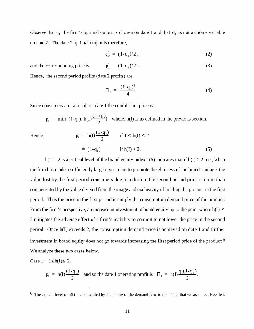
Observe that q1 the firm’s optimal output is chosen on date 1 and that q1 is not a choice variable

on date 2. The date 2 optimal output is therefore,

q2* = (1-q1)/2 , (2)

and the corresponding price is p2* = (1-q1)/2 . (3)

Hence, the second period profits (date 2 profits) are

Π2 = (1-q1)2

4. (4)

Since consumers are rational, on date 1 the equilibrium price is

p1 = min{(1-q1), h(I)(1-q1)

2} where, h(I) is as defined in the previous section.

Hence, p1 = h(I)(1-q 1)

2if 1 ≤ h(I) ≤ 2

= (1-q1) if h(I) > 2. (5)

h(I) = 2 is a critical level of the brand equity index. (5) indicates that if h(I) > 2, i.e., when

the firm has made a sufficiently large investment to promote the eliteness of the brand’s image, the

value lost by the first period consumers due to a drop in the second period price is more than

compensated by the value derived from the image and exclusivity of holding the product in the first

period. Thus the price in the first period is simply the consumption demand price of the product.

From the firm’s perspective, an increase in investment in brand equity up to the point where h(I) ≤

2 mitigates the adverse effect of a firm’s inability to commit to not lower the price in the second

period. Once h(I) exceeds 2, the consumption demand price is achieved on date 1 and further

investment in brand equity does not go towards increasing the first period price of the product.8

We analyze these two cases below.

Case 1 : 1≤h(I)≤ 2.

p1 = h(I)(1-q 1)

2 and so the date 1 operating profit is Π1 = h(I)

q1(1-q1 )

2.

8 The critical level of h(I) = 2 is dictated by the nature of the demand function p = 1- q, that we assumed. Needless

12

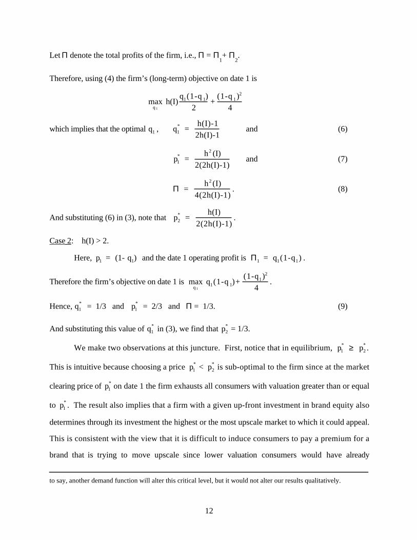
Let Π denote the total profits of the firm, i.e., Π = Π1+ Π

2.

Therefore, using (4) the firm’s (long-term) objective on date 1 is

maxq 1

h(I)q1(1-q 1)

2+

(1-q 1)2

4

which implies that the optimal q1 , q1* =

h(I)-1

2h(I)-1and (6)

p1* =

h2 (I)

2(2h(I)-1)and (7)

Π = h2 (I)

4(2h(I)-1). (8)

And substituting (6) in (3), note that p2* =

h(I)

2(2h(I)-1).

Case 2 : h(I) > 2.

Here, p1 = (1- q1) and the date 1 operating profit is Π1 = q1(1-q1) .

Therefore the firm’s objective on date 1 is maxq 1

q1(1-q 1)+(1-q1)2

4.

Hence, q1* = 1/3 and p1

* = 2/3 and Π = 1/3. (9)

And substituting this value of q1* in (3), we find that p2

* = 1/3.

We make two observations at this juncture. First, notice that in equilibrium, p1* ≥ p2

* .

This is intuitive because choosing a price p1*

< p2

*

is sub-optimal to the firm since at the market

clearing price of p1*

on date 1 the firm exhausts all consumers with valuation greater than or equal

to p1* . The result also implies that a firm with a given up-front investment in brand equity also

determines through its investment the highest or the most upscale market to which it could appeal.

This is consistent with the view that it is difficult to induce consumers to pay a premium for a

brand that is trying to move upscale since lower valuation consumers would have already

to say, another demand function will alter this critical level, but it would not alter our results qualitatively.

13

purchased the product at the earlier price thereby reducing the brand’s image appeal and eliteness.

Thus, we invariably see firms move upscale only under a completely new brand identity.9

Second, observe that the optimal price and the firm’s profits are both independent of h(I)

when h(I) > 2, but are increasing functions of h(I) otherwise. Investment in brand equity enables

the firm to achieve a higher first period price for a firm that is unable to commit to not lower the

second period price. However, this role of brand equity is redundant once h(I) is greater than 2, a

point beyond which the first period price for the product is dictated by the consumption demand for

the product. Therefore, a very large investment in brand equity, such that h(I) > 2, is not useful to

the firm as it does not contribute to increasing the firm’s operating profits.

Proposition 1: When the firm is unable to commit to a price path, its operating profits are

increasing with investment in brand equity for small levels of I, and is independent of brand equity

at sufficiently high levels of I.

Proof: Case 1 : I such that 1 ≤ h(I) ≤ 2.

From (8) the profits from operations Π = h2 (I)

4(2h(I)-1)

and ∂Π∂I

= 1

4{2h(I) ′ h (I)[2h(I)-1]-2h 2 (I) ′ h (I)

[2h(I)-1]2}

or equivalently,∂Π∂I

= h(I) ′ h (I)[h(I)-1]

2[2h(I)-1]2

≥ 0 since 1 ≤ h(I), and ′ h (I) > 0.

Case 2 : I such that h(I) > 2.

From (9) the firms total operating profit is 1/3, and is independent of the firm’s level of investment

in brand equity. ♦

Although, in the above proposition, we only consider the firm’s operating profits, which

ignores the up-front investment in brand equity (the cost), Proposition 1 does establish the

9 A case in point is the line of luxury cars introduced by Honda, Toyota, and Nissan, who chose to create

14

necessary condition for the viability of any investment in brand equity. Below we show that for

each dollar of investment in brand equity, as long as the marginal increase in the brand equity index

h(I) is sufficiently high, a positive level of investment in brand equity that improves the brand’s

image is optimal to the firm.

Proposition 2: When the firm is unable to commit to a price path, a sufficient condition for a

positive investment in brand equity to be optimal is that h(I) satisfies the inequality (10) at some I

such that 1 < h(I) ≤ 2.

(h(I)-1)2

4(2h(I)-1) > I (10)

Proof: In what follows, we sometimes use h in the place of h(I) to reduce notational clutter.

From (8) and (9) Π = h2

4(2h -1)when 1 ≤ h(I) ≤ 2.

Π = 1/3 when h(I) > 2.

The firm’s objective on date 0 is to select I such that

maxI

Π - I

Since Π = 1/3 when h(I) = 2, and is a constant ∀ I such that h(I) > 2, (Π - I) is decreasing ∀ I

where h(I) > 2. Therefore, the optimal value of I that maximizes (Π - I) lies in the range where 1

≤ h(I) ≤ 2.

Therefore, the date 0 objective is maxI

h2

4(2h-1) - I

Since h(0) = 1, the net profits for the firm is 1/4 when the investment in brand equity is zero. For

a positive level of investment to be optimal it must be the case that

h2

4(2h -1) - I > 1/ 4 for some I > 0.

That is, h2 − 2h +1

4(2h -1) - I > 0

completely new identities viz., Acura, Lexus, and Infiniti, when they decided to target a more upscale market.

15

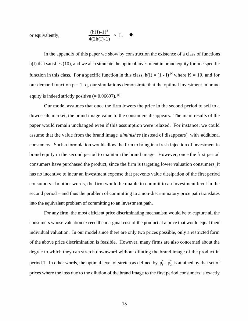
or equivalently, (h(I)-1)2

4(2h(I)-1) > I . ♦

In the appendix of this paper we show by construction the existence of a class of functions

h(I) that satisfies (10), and we also simulate the optimal investment in brand equity for one specific

function in this class. For a specific function in this class, h(I) = (1 - I)-K where K = 10, and for

our demand function p = 1- q, our simulations demonstrate that the optimal investment in brand

equity is indeed strictly positive (= 0.06697).10

Our model assumes that once the firm lowers the price in the second period to sell to a

downscale market, the brand image value to the consumers disappears. The main results of the

paper would remain unchanged even if this assumption were relaxed. For instance, we could

assume that the value from the brand image diminishes (instead of disappears) with additional

consumers. Such a formulation would allow the firm to bring in a fresh injection of investment in

brand equity in the second period to maintain the brand image. However, once the first period

consumers have purchased the product, since the firm is targeting lower valuation consumers, it

has no incentive to incur an investment expense that prevents value dissipation of the first period

consumers. In other words, the firm would be unable to commit to an investment level in the

second period – and thus the problem of committing to a non-discriminatory price path translates

into the equivalent problem of committing to an investment path.

For any firm, the most efficient price discriminating mechanism would be to capture all the

consumers whose valuation exceed the marginal cost of the product at a price that would equal their

individual valuation. In our model since there are only two prices possible, only a restricted form

of the above price discrimination is feasible. However, many firms are also concerned about the

degree to which they can stretch downward without diluting the brand image of the product in

period 1. In other words, the optimal level of stretch as defined by p1* - p2

* is attained by that set of

prices where the loss due to the dilution of the brand image to the first period consumers is exactly

16

offset by the higher utility from the exclusivity of holding the product in the first period. The

higher is the difference between the two prices, the greater is the market coverage as more lower

valuation consumers buy the product. Firms are thus interested in being able to stretch as far down

as they can without adversely affecting their brand image and their first period prices. Below we

demonstrate that for firms that are concerned about the dilution of brand image but also have a

desire to stretch downwards as a means of achieving a second order objective such as market

coverage, higher levels of investment in brand equity enables them to stretch deeper.

Proposition 3: The ability of a profit maximizing firm to stretch downward is increasing in its

investment in brand equity if and only if the investment I is such that h(I) ≤ 2.

Proof: We prove the proposition by establishing that ∂(p1

* -p 2* )

∂I > 0 if and only if h(I)≤ 2.

Using (3) and (6), p2* =

h(I)

2(2h(I)-1) when h(I) ≤ 2.

Therefore, from (7) p1* - p2

* = h(h(I)-1)

2(2h(I)-1)if h(I) ≤ 2

and using (3) and (9)

p1* - p2

* = 1

3if h(I) > 2.

Observe that when h(I) ≤ 2, ∂(p1

* -p 2* )

∂I > 0 since h(I) is increasing in I.

Also when h(I) > 2, ∂(p1

* -p 2* )

∂I = 0. This establishes the proposition. ♦

In the next section, we consider the case where the firm has the ability to credibly commit to a non-

discriminatory price path. We demonstrate that investment in brand equity is unlike an investment

in a tangible aspect of the product, in that, it mitigates the losses that arise from a firm’s inability to

commit to a price path, and to some extent substitutes for the firm’s commitment ability. We show

10 The optimal investment in brand equity is positive even for h(I) with other values of K. The results of thosesimulations are not included in the appendix, but are available from the authors upon request

17

this by comparing the case where the firm is unable to commit to a price path to the case where the

firm is able to commit to a non-discriminatory price path – and then establishing that the benefit

from an investment in brand equity is greater when the firm is unable to commit than when it is

able to commit to a price path.

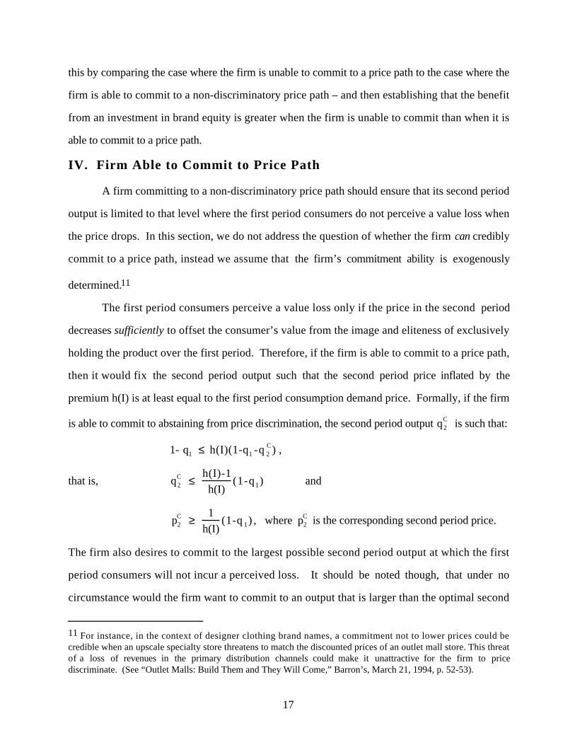
IV. Firm Able to Commit to Price Path

A firm committing to a non-discriminatory price path should ensure that its second period

output is limited to that level where the first period consumers do not perceive a value loss when

the price drops. In this section, we do not address the question of whether the firm can credibly

commit to a price path, instead we assume that the firm’s commitment ability is exogenously

determined.11

The first period consumers perceive a value loss only if the price in the second period

decreases sufficiently to offset the consumer’s value from the image and eliteness of exclusively

holding the product over the first period. Therefore, if the firm is able to commit to a price path,

then it would fix the second period output such that the second period price inflated by the

premium h(I) is at least equal to the first period consumption demand price. Formally, if the firm

is able to commit to abstaining from price discrimination, the second period output q2C

is such that:

1- q1 ≤ h(I)(1-q1 -q 2C) ,

that is, q2C ≤

h(I)-1

h(I)(1-q1) and

p2C ≥

1

h(I)(1-q 1) , where p2

C is the corresponding second period price.

The firm also desires to commit to the largest possible second period output at which the first

period consumers will not incur a perceived loss. It should be noted though, that under no

circumstance would the firm want to commit to an output that is larger than the optimal second

11 For instance, in the context of designer clothing brand names, a commitment not to lower prices could becredible when an upscale specialty store threatens to match the discounted prices of an outlet mall store. This threatof a loss of revenues in the primary distribution channels could make it unattractive for the firm to pricediscriminate. (See “Outlet Malls: Build Them and They Will Come,” Barron’s, March 21, 1994, p. 52-53).

18

period output under the no-commitment case (i.e., the unconstrained case), even if at that larger

output the first period consumers still perceive no loss. Comparing the commitment equilibrium

second period output q2C with (2), the output q2

* when the firm is unable to commit, we see that

q2C ≤ q2

* when 1≤ h(I)≤ 2

This implies that for any value 1≤ h(I)≤ 2, the brand equity index is not high enough to offset the

perceived loss to the first period consumers if the firm produces the unconstrained optimum output

in the second period. Thus, in this case, the firm has to commit to a quantity that is strictly lower

than the unconstrained optimal quantity. Since q2* is the unconstrained optimum output for the

firm on date 2, the commitment that the firm would make is:

q2C = min {

(h(I)-1)

h(I)(1-q1), q2

*}

i.e., the firm would not raise its second period output beyond q2* , even when it is able to commit to

a larger output without being penalized (in the date 1 price) by the first period consumers.

Hence from (2), q2C = min {

(h(I)-1)

h(I)(1-q1),

(1-q 1)

2} and equivalently,

p2C = max {

(1-q1)

h(I),

(1-q1 )

2}

This implies Π2 = h(I)-1

h2(I)(1-q1)2 if h(I) ≤ 2

= (1-q 1)2

4if h(I) > 2. (11)

and from (1) p1 = min {(1-q1), h(I) Max {(1- q1)

h(I),

(1-q1)

2}}

which implies that p1 = min {(1-q1), (1-q1)} if h(I) ≤ 2

= min {(1-q 1), h(I)(1-q 1)

2} if h(I) > 2.

Thus, p1 = (1- q1) ∀ h(I).

19

The intuition behind the last equation is straightforward. When the firm is able to credibly commit

to protecting its first period consumers from any value loss, the first period price is no longer a

function of the expected second period price. In other words, the first period price is simply the

consumption demand price of date 1.

Therefore, Π1 = q1(1-q1) (12)

and from (11) and (12) Π = q 1(1-q1) + h(I)-1

h2 (I)(1-q1 )2 if h(I) ≤ 2

= q1(1 -q1) + (1-q1)2

4if h(I) > 2.

Hence when h(I) ≤ 2, the date 1 maximization problem for the firm is:

maxq 1

q1(1-q 1) + h(I)-1

h2(I)(1-q 1)2

which implies the optimal q1C =

(h2 -2h +2)

2(h2 -h +1),

p1C =

h2

2(h2 -h+1)and

hence, Π = h2

4(h 2 - h+1). (13)

And when h(I) > 2, the optimal q1C = 1/3, p1

C

= 2/3, and therefore, Π = 1/3. (14)

Proposition 4: The profits of a firm that is able to commit to preserving the first period

consumers’ value is at least as high as that of a firm which is unable to commit to a price path.

Proof: When 1 < h(I) < 2, from (8) the profits under the no commitment case is

Π = h2

4(2h -1);

comparing this with (13), the profits when the firm is able to commit, we see that the difference is

h2

4(h 2 -h+1) -

h2

4(2h-1)

20

= h2 (2h-1)-h 2(h 2 - h+1)

4(h2 - h+1)(2h -1)

= - h2 (h-2)(h -1)

4(h2 - h+1)(2h -1)

> 0 since, 1 < h < 2.

Finally, the result is established by making two observations. When h(I) = 1 comparing

(8) and (13) shows that commitment profits are equal to the no-commitment profits; and when h(I)

> 2 comparing (9) and (14) shows that the maximization problems, and hence, the optimal

solutions are the same under the commitment and no-commitment cases. ♦

The intuition behind proposition 4 is straightforward. The profits to a firm from price

discriminating across time is determined by the size of the premium h(I) that the brand can demand.

For any given level of the expected second period price, the first period consumers are willing to

pay a higher price as h(I) increases. Proposition 4 confirms our intuition that the profits when the

firm is able to commit to protecting the first period consumers’ value is always at least as high as

that when the firm is unable to commit. The ability to commit fails to have incremental value only

when the investment in brand equity is high enough such that h(I) > 2. This is because even for a

firm that is unable to commit, if investment in brand equity is sufficiently high, the value derived

(from exclusively owning an elite brand) by the first period consumers is greater than the perceived

loss when the firm selects its optimal second period price. Thus there are no adverse consequences

from a firm’s inability to commit and therefore, the ability to commit offers no special benefit when

h(I) > 2. In other words, if a firm’s ability to commit can only be obtained at a further cost then it

is sub-optimal for the firm to pay for this ability, if it has invested a sufficiently large amount in

enhancing the eliteness of its brand image.

Finally, the case when h(I) = 1 requires some explanation. h(I) = 1 when I = 0. This

pertains to the scenario where the firm makes no investment in brand equity. In this case the first

period consumers associate no premium with owning the product exclusively over the first period.

21

Therefore, the equilibrium price in the first period is simply the minimum of the consumption

demand price or the expected second period price. As we demonstrate in section 2, the optimal

strategy for the firm in this case is to sell all its output only on date 2, since no price p > 0 would

be accepted on date 1. By producing and selling its output only on date 2, the firm renders the

need for committing to a price path irrelevant, and therefore the ability to commit has no

incremental value. However, as we show below in proposition 5, I = 0 is overall a sub-optimal

investment decision for the firm as long as the brand equity index h(I) is sufficiently rapidly

increasing in I.

Proposition 5: When the firm is able to commit to a price path, a sufficient condition for a

positive investment in brand equity to be optimal is that h(I) satisfies the inequality (15) at some I

such that 1 < h(I) ≤ 2.

h(I)-1

4(h 2 -h+1) > I . (15)

Proof: From (13) and (14)

Π = h2

4(h 2 - h+1)when 1 ≤ h(I) ≤ 2.

Π = 1/3 when h(I) > 2.

The firm’s objective on date 0 is to select I such that

maxI

Π - I

Since Π = 1/3 when h(I) = 2, and is a constant ∀ I such that h(I) > 2, (Π - I) is decreasing ∀ I

such that h(I) > 2. Therefore, the optimal value of I that maximizes (Π - I) lies in the range where

1 ≤ h(I) ≤ 2.

Therefore the date 0 objective is maxI

h2

4(h2 -h +1) - I

Since h(0) = 1, the net profits for the firm is 1/4 when the investment in brand equity is zero. For

a positive level of investment to be optimal it must be the case that

22

h2

4(h 2 -h+1) - I > 1/ 4 for some I > 0.

i.e., h -1

4(h 2 -h+1) - I > 0 for some I such that 1 < h(I) ≤ 2. ♦

As before, in the appendix of this paper we show by construction the existence of a class of

functions h(I) that satisfies (15). Using a specific function in this class, we also simulate the

optimal investment in brand equity for a firm that is able to commit to a price path. Our simulations

demonstrate that when h(I) = (1 - I)-K where K = 10, and for our demand function p = 1- q, the

optimal investment in brand equity is strictly positive (= 0.03974) even when the firm is able to

commit to a price path.

The marginal benefit from investment in brand equity is higher for a firm whose first period

price is adversely affected by the anticipated drop in the second period price, that is, for a firm that

is unable to commit to a price path. Therefore, the optimal investment in brand equity should be

higher when the firm is unable to commit not to price discriminate than when it is able to commit.

In fact, as can be seen from the example simulated in the appendix, the optimal investment in brand

equity when the firm is unable to commit is about 68% higher than in the case where the firm is

able to commit to a price path. This shows that investment is brand equity is unlike other

investments that affect the objective quality of the product, in that it affects a firm’s value

differently when the firm is able to commit to a price path than when it is unable to commit. We

demonstrate the result formally in proposition 6 below.

Proposition 6: The optimal investment in brand equity is greater when the firm is unable to

commit not to price discriminate than when it is able to commit to a non-discriminatory price path.

Proof: Let I* be the optimal investment when the firm is unable to commit. From (8) and (9), I*

maximizes the following:

maxI

h2

4(2h-1) - I where I is such that 1 ≤ h(I) ≤ 2.

23

From the first order condition for the above objective, I* satisfies the condition that

h ′ h (h -1)

2(2h -1)2 − 1 = 0 (16)

Let I** be the optimal investment when the firm is able to commit. From (13) and (14), I**

maximizes the following

maxI

h2

4(h2 -h +1) - I where I is such that 1 ≤ h(I) ≤ 2.

From the first order condition for the above objective, I** satisfies the condition that

h ′ h (2-h)

4(h 2 -h+1)2 − 1 = 0 (17)

We prove that I* ≥ I** by showing that the left hand side of (16) is strictly greater than zero when

evaluated at I**. In other words, we demonstrate that to attain I*, the optimal investment in brand

equity when the firm is unable to commit, the firm has to increase its investment to a point beyond

I**. From (17)

h ′ h (2-h)

4(h 2 -h+1)2 = 1 at I = I**.

Therefore, the left hand side of (16) becomes

h ′ h (h -1)

2(2h -1)2 −

h ′ h (2- h)

4(h2 -h +1)2 (18)

when I = I**. Expression (18) is greater than or equal to 0 if

4(h 2 − h +1)2(h ′ h )(h −1) − 2(2h −1)2 (h ′ h )(2 − h) ≥ 0 .

This is equivalent to showing that

2h ′ h [2(h 2 − h +1)2(h −1) − (2h −1)2(2 − h)] ≥ 0 ,

which is indeed the case since, 1 ≤ h(I) ≤ 2, and ′ h (I) > 0. ♦

24

The intuition behind the above proposition is fundamental to the focus of this paper. We

show that investment in brand equity provides additional value for a firm that is unable to commit

not to price discriminate compared to a firm that is able to commit to a non-discriminatory price

path. In other words, an investment in brand equity does not just increase a firm’s revenues in

ways similar to investments in tangible aspects of the product, such as an investment in quality

improvements or R&D. It serves as a mechanism by which a firm that does not have an

exogenous ability to commit can offset the loss to the first period (high valuation) consumers when

the price decreases in the second period. Thus, it serves as bonding mechanism between the firm

and the high valuation consumers.

V. Conclusions

We model the incentives of a firm to sell an image or prestige good in the first period at a

high price to an upscale market, and in the subsequent period lower the price and target a more

downscale market. We argue that this strategy results in a perceived loss to the first period

consumers due to the decline in exclusivity of the product when it is later sold at a lower price to a

larger and less affluent market. We assume that consumers rationally anticipate such price

discrimination behavior by the firm, and hence, pay less for the firm’s product in the first period.

In particular, the equilibrium price that consumers pay in the first period is the lower of the first

period consumption demand price or the expected second period price inflated to reflect the added

value from the exclusivity of owning the product in the first period. This latter adjustment may be

viewed as the premium consumers are willing to pay over the expected second period price in order

to hold an exclusive product in the first period, and is a function of the investment made by the

firm towards promoting the eliteness of its brand’s image. In other words, the adjustment is an

increasing function of the degree of eliteness that is indicated by the firm’s investment in brand

equity. We show that investment in brand equity helps mitigate the effect of the perceived loss in

value faced by the first period consumers when a firm is unable to credibly commit to a non-

discriminatory price path.

The key insights of the analysis using our model are as follows:

25

Higher is the up-front investment in brand equity higher is the value from the exclusivity of

owning the product in the first period, and higher is the premium over the expected second period

price that first period consumers are willing to pay. The firm’s operating profits as well as the

profits net of the investment in brand equity are an increasing function of the investment up to a

certain threshold of the brand equity index. Also, a firm’s ability to price discriminate increases

with investment in brand equity. That is, the difference between the first and the second period

price is an increasing function of the firm’s up-front investment in brand equity.

More importantly, we show that investment in brand equity is unlike an investment in a

tangible aspect of the product, in that, it mitigates the losses that arise from a firm’s inability to

commit to a price path. We establish this result by demonstrating that although a positive level of

investment in brand equity is optimal irrespective of a firm’s ability to commit to a price path, the

benefit from the investment is higher when the firm is unable to commit than when it is able to

commit to a non-discriminatory price path.

We also show that the profits when the firm is able to commit to a price path (i.e., commit

to protecting the first period consumers from any perceived loss) is always at least as high as that

when the firm is unable to commit. The ability to commit to a price path offers no special benefits

only when investment in brand equity is sufficiently large. This is because when investment in

brand equity is large, the value derived from the exclusivity of holding the product in the first

period offsets the perceived loss arising from the lower second period price.

26

Appendix

In this appendix we provide an example of a class of functions that satisfies the inequalities

(10) and (15). It may be easily verified that h(I) = (1 - I)-K where K > 4, satisfies (15) and the

same class of functions satisfies (10) when K > 8. Below we present the values of h(I) and the net

profits of the firm for different levels of I, the investment in brand equity. In each case the level of

investment that maximizes net profits is highlighted in boldface.

Investment (I) K h(I)Net Profits (Π - I) Net Profits (Π - I)

Firm unable to commit Firm able to commit

0.00000 10 1.000000 0.250000 0.250000

0.00500 10 1.051403 0.245599 0.257192

0.01000 10 1.105727 0.242307 0.263665

0.01500 10 1.163155 0.240018 0.269283

0.02000 10 1.223881 0.238655 0.273933

0.02500 10 1.288113 0.238166 0.277532

0.03000 10 1.356072 0.238513 0.280031

0.03500 10 1.427996 0.239674 0.281410

0.03974 10 1.500000 0.241515 0.281693

0.04500 10 1.584770 0.244404 0.280876

0.05000 10 1.670183 0.247978 0.279056

0.05500 10 1.760686 0.252374 0.276293

0.06000 10 1.856613 0.257612 0.272672

0.06500 10 1.958321 0.263719 0.268283

0.06690 10 1.998564 0.266274 0.266433

0.06697 10 2.000000 0.266366 0.266366

0.06700 10 2.000707 0.266333 0.266333

0.07000 10 2.066191 0.263333 0.263333

0.08000 10 2.302087 0.253333 0.253333

0.09000 10 2.567947 0.243333 0.243333

0.10000 10 2.867972 0.233333 0.233333

0.15000 10 5.079380 0.183333 0.183333

0.20000 10 9.313226 0.133333 0.133333

27

References

Aaker, David, “The Value of Brand Equity,” Journal of Business Strategy, (1991), 27-32.

Besanko, David and Wayne L. Winston, “Optimal Price Skimming by a Monopolist FacingRational Customers,” Management Science, 36 (May 1990), 555-567.

Bulow, Jeremy I., “Durable-Goods Monopolists,” Journal of Political Economy, 90 (1982), 314-332.

Bulow, Jeremy I., “An Economic Theory of Planned Obsolescence,” Quarterly Journal ofEconomics, 51 (1986), 729-750.

Coase, Ronald, “Durability and Monopoly,” Journal of Law and Economics, 15 (1972), 143-149.

Furquhar, Peter, H., “Managing Brand Equity,” Marketing Research, 1 (September 1989), 24-33.

Levinthal, Daniel A., and Devavrat Purohit, “Durable Goods and Product Obsolescence,”Marketing Science, 8 (Winter 1989), 35-56.

Moorthy, K. Sridhar, and I.P.L. Png, “Market Segmentation, Cannibalization and the Timing ofProduct Introductions,” Management Science, 38 (March 1992), 345-359.

Moorthy, K. Sridhar, and H. Zhao, “Advertising and Quality: An Empirical Analysis,” WorkingPaper, 1996, University of Rochester, Rochester, NY.

Stokey, Nancy, “Intertemporal Price Discrimination,” Quarterly Journal of Economics, 93 (August1979), 355-371.

Stokey, Nancy, “Rational Expectations and Durable Goods Pricing,” Bell Journal of Economics,12 (1981), 112-128.

Tirole, Jean, The Theory of Industrial Organization, The MIT Press, Cambridge, MA, 1990.

Waldman, Michael, Durable Goods Pricing When Quality Matters,” Journal of Business , 69(1996), 489-510.