international school for advanced studies trieste u. bruzzo
TRANSCRIPT
INTERNATIONAL SCHOOL
FOR ADVANCED STUDIES
Trieste
U. Bruzzo
INTRODUCTION TO
ALGEBRAIC TOPOLOGY AND
ALGEBRAIC GEOMETRY
Notes of a course delivered during the academic year 2002/2003
La filosofia e scritta in questo grandissimo libro che continuamenteci sta aperto innanzi a gli occhi (io dico l’universo), ma non si puointendere se prima non si impara a intender la lingua, e conoscer icaratteri, ne’ quali e scritto. Egli e scritto in lingua matematica, ei caratteri son triangoli, cerchi, ed altre figure geometriche, senzai quali mezi e impossibile a intenderne umanamente parola; senzaquesti e un aggirarsi vanamente per un oscuro laberinto.
Galileo Galilei (from “Il Saggiatore”)
i
Preface
These notes assemble the contents of the introductory courses I have been giving atSISSA since 1995/96. Originally the course was intended as introduction to (complex)algebraic geometry for students with an education in theoretical physics, to help them tomaster the basic algebraic geometric tools necessary for doing research in algebraicallyintegrable systems and in the geometry of quantum field theory and string theory. Thismotivation still transpires from the chapters in the second part of these notes.
The first part on the contrary is a brief but rather systematic introduction to twotopics, singular homology (Chapter 2) and sheaf theory, including their cohomology(Chapter 3). Chapter 1 assembles some basics fact in homological algebra and developsthe first rudiments of de Rham cohomology, with the aim of providing an example tothe various abstract constructions.
Chapter 5 is an introduction to spectral sequences, a rather intricate but very pow-erful computation tool. The examples provided here are from sheaf theory but thiscomputational techniques is also very useful in algebraic topology.
I thank all my colleagues and students, in Trieste and Genova and other locations,who have helped me to clarify some issues related to these notes, or have pointed outmistakes. In this connection special thanks are due to Fabio Pioli. Most of Chapter 3 isan adaptation of material taken from [2]. I thank my friends and collaborators ClaudioBartocci and Daniel Hernandez Ruiperez for granting permission to use that material.I thank Lothar Gottsche for useful suggestions and for pointing out an error and thestudents of the 2002/2003 course for their interest and constant feedback.
Genova, 4 December 2004

Contents
Part 1. Algebraic Topology 1
Chapter 1. Introductory material 31. Elements of homological algebra 32. De Rham cohomology 73. Mayer-Vietoris sequence in de Rham cohomology 104. Elementary homotopy theory 11
Chapter 2. Singular homology theory 171. Singular homology 172. Relative homology 253. The Mayer-Vietoris sequence 284. Excision 32
Chapter 3. Introduction to sheaves and their cohomology 371. Presheaves and sheaves 372. Cohomology of sheaves 433. Sheaf cohomology 52
Chapter 4. More homological algebra 57
Chapter 5. Spectral sequences 591. Filtered complexes 592. The spectral sequence of a filtered complex 603. The bidegree and the five-term sequence 644. The spectral sequences associated with a double complex 655. Some applications 68
Part 2. Introduction to algebraic geometry 73
Chapter 6. Complex manifolds and vector bundles 751. Basic definitions and examples 752. Some properties of complex manifolds 783. Dolbeault cohomology 794. Holomorphic vector bundles 795. Chern class of line bundles 83
iii
iv CONTENTS
6. Chern classes of vector bundles 857. Kodaira-Serre duality 878. Connections 88
Chapter 7. Divisors 931. Divisors on Riemann surfaces 932. Divisors on higher-dimensional manifolds 1003. Linear systems 1014. The adjunction formula 103
Chapter 8. Algebraic curves I 1071. The Kodaira embedding 1072. Riemann-Roch theorem 1103. Some general results about algebraic curves 111
Chapter 9. Algebraic curves II 1171. The Jacobian variety 1172. Elliptic curves 1223. Nodal curves 126
Bibliography 131
Part 1
Algebraic Topology

CHAPTER 1
Introductory material
The aim of the first part of these notes is to introduce the student to the basics ofalgebraic topology, especially the singular homology of topological spaces. The futuredevelopments we have in mind are the applications to algebraic geometry, but alsostudents interested in modern theoretical physics may find here useful material (e.g.,the theory of spectral sequences).
As its name suggests, the basic idea in algebraic topology is to translate problemsin topology into algebraic ones, hopefully easier to deal with.
In this chapter we give some very basic notions in homological algebra and thenintroduce the fundamental group of a topological space. De Rham cohomology is in-troduced as a first example of a cohomology theory, and is homotopic invariance isproved.
1. Elements of homological algebra
1.1. Exact sequences of modules. Let R be a ring, and let M , M ′, M ′′ beR-modules. We say that two R-module morphisms i : M ′ → M , p : M → M ′′ form anexact sequence of R-modules, and write
0→M ′i−−→M
p−−→M ′′ → 0 ,
if i is injective, p is surjective, and ker p = Im i.
Example 1.1. Set R = Z, the ring of integers (recall that Z-modules are just abeliangroups), and consider the sequence
(1.1) 0→ Z i−−→C exp−−→C∗ → 1
where i is the inclusion of the integers into the complex numbers C, while C∗ = C−0is the multiplicative group of nonzero complex numbers. The morphism exp is definedas exp(z) = e2πiz. The reader may check that this sequence is exact.
A morphism of exact sequences is a commutative diagram
0 −−−−→ M ′ −−−−→ M −−−−→ M ′′ −−−−→ 0y y y0 −−−−→ N ′ −−−−→ N −−−−→ N ′′ −−−−→ 0
of R-module morphisms whose rows are exact.
3
4 1. INTRODUCTORY MATERIAL
1.2. Differential complexes. Let R be a ring, and M an R-module.
Definition 1.2. A differential on M is a morphism d : M →M of R-modules suchthat d2 ≡ d d = 0. The pair (M,d) is called a differential module.
The elements of the spaces M , Z(M,d) ≡ ker d and B(M,d) ≡ Im d are calledcochains, cocycles and coboundaries of (M,d), respectively. The condition d2 = 0 impliesthat B(M,d) ⊂ Z(M,d), and the R-module
H(M,d) = Z(M,d)/B(M,d)
is called the cohomology group of the differential module (M,d). We shall often writeZ(M), B(M) and H(M), omitting the differential d when there is no risk of confusion.
Let (M,d) and (M ′, d′) be differential R-modules.
Definition 1.3. A morphism of differential modules is a morphism f : M →M ′ ofR-modules which commutes with the differentials, f d′ = d f .
A morphism of differential modules maps cocycles to cocycles and coboundaries tocoboundaries, thus inducing a morphism H(f) : H(M)→ H(M ′).
Proposition 1.4. Let 0 → M ′i−−→M
p−−→M ′′ → 0 be an exact sequence of dif-ferential R-modules. There exists a morphism δ : H(M ′′) → H(M ′) (called connectingmorphism) and an exact triangle of cohomology
H(M)H(p)
// H(M ′′)
δyyttttttttt
H(M ′)
H(i)
OO
Proof. The construction of δ is as follows: let ξ′′ ∈ H(M ′′) and let m′′ be acocycle whose class is ξ′′. If m is an element of M such that p(m) = m′′, we havep(d(m)) = d(m′′) = 0 and then d(m) = i(m′) for some m′ ∈ M ′ which is a cocycle.Now, the cocycle m′ defines a cohomology class δ(ξ′′) in H(M ′), which is independent ofthe choices we have made, thus defining a morphism δ : H(M ′′)→ H(M ′). One provesby direct computation that the triangle is exact.
The above results can be translated to the setting of complexes of R-modules.
Definition 1.5. A complex of R-modules is a differential R-module (M•, d) whichis Z-graded, M• =
⊕n∈ZM
n, and whose differential fulfills d(Mn) ⊂ Mn+1 for everyn ∈ Z.
We shall usually write a complex of R-modules in the more pictorial form
. . .dn−2−−→Mn−1 dn−1−−→Mn dn−−→Mn+1 dn+1−−→ . . .
1. HOMOLOGICAL ALGEBRA 5
For a complex M• the cocycle and coboundary modules and the cohomology groupsplit as direct sums of terms Zn(M•) = ker dn, Bn(M•) = Im dn−1 and Hn(M•) =Zn(M•)/Bn(M•) respectively. The groups Hn(M•) are called the cohomology groupsof the complex M•.
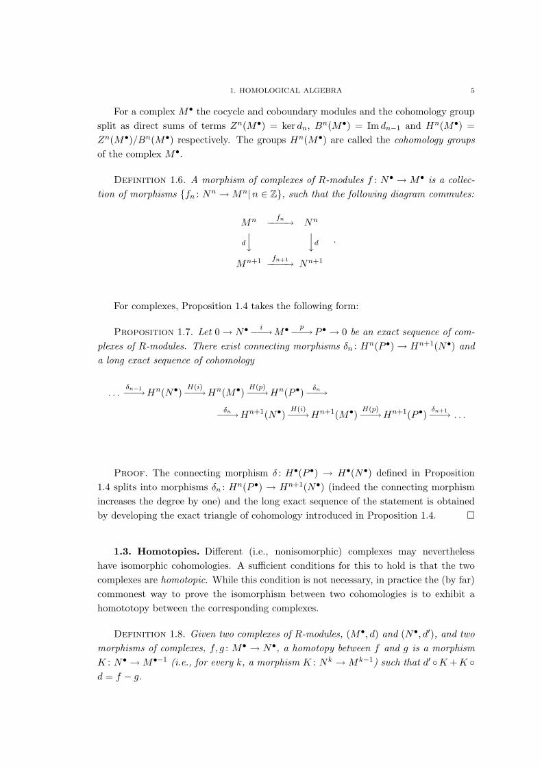
Definition 1.6. A morphism of complexes of R-modules f : N• → M• is a collec-tion of morphisms fn : Nn →Mn|n ∈ Z, such that the following diagram commutes:
Mn fn−−−−→ Nn
d
y ydMn+1 fn+1−−−−→ Nn+1
.
For complexes, Proposition 1.4 takes the following form:
Proposition 1.7. Let 0→ N•i−−→M•
p−−→P • → 0 be an exact sequence of com-plexes of R-modules. There exist connecting morphisms δn : Hn(P •)→ Hn+1(N•) anda long exact sequence of cohomology
. . .δn−1−−→Hn(N•)
H(i)−−→Hn(M•)H(p)−−→Hn(P •) δn−−→
δn−−→Hn+1(N•)H(i)−−→Hn+1(M•)
H(p)−−→Hn+1(P •)δn+1−−→ . . .
Proof. The connecting morphism δ : H•(P •) → H•(N•) defined in Proposition1.4 splits into morphisms δn : Hn(P •) → Hn+1(N•) (indeed the connecting morphismincreases the degree by one) and the long exact sequence of the statement is obtainedby developing the exact triangle of cohomology introduced in Proposition 1.4.
1.3. Homotopies. Different (i.e., nonisomorphic) complexes may neverthelesshave isomorphic cohomologies. A sufficient conditions for this to hold is that the twocomplexes are homotopic. While this condition is not necessary, in practice the (by far)commonest way to prove the isomorphism between two cohomologies is to exhibit ahomototopy between the corresponding complexes.
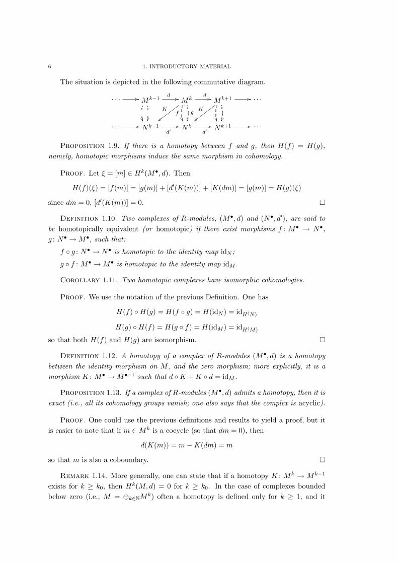
Definition 1.8. Given two complexes of R-modules, (M•, d) and (N•, d′), and twomorphisms of complexes, f, g : M• → N•, a homotopy between f and g is a morphismK : N• →M•−1 (i.e., for every k, a morphism K : Nk →Mk−1) such that d′ K+K d = f − g.
6 1. INTRODUCTORY MATERIAL
The situation is depicted in the following commutative diagram.
. . . // Mk−1
d // Mk
f
g
d //
K
wwwwwwwwMk+1
//
K
wwwwwwww. . .
. . . // Nk−1d′// Nk
d′// Nk+1 // . . .
Proposition 1.9. If there is a homotopy between f and g, then H(f) = H(g),namely, homotopic morphisms induce the same morphism in cohomology.
Proof. Let ξ = [m] ∈ Hk(M•, d). Then
H(f)(ξ) = [f(m)] = [g(m)] + [d′(K(m))] + [K(dm)] = [g(m)] = H(g)(ξ)
since dm = 0, [d′(K(m))] = 0.
Definition 1.10. Two complexes of R-modules, (M•, d) and (N•, d′), are said tobe homotopically equivalent (or homotopic) if there exist morphisms f : M• → N•,g : N• →M•, such that:
f g : N• → N• is homotopic to the identity map idN ;
g f : M• →M• is homotopic to the identity map idM .
Corollary 1.11. Two homotopic complexes have isomorphic cohomologies.
Proof. We use the notation of the previous Definition. One has
H(f) H(g) = H(f g) = H(idN ) = idH(N)
H(g) H(f) = H(g f) = H(idM ) = idH(M)
so that both H(f) and H(g) are isomorphism.
Definition 1.12. A homotopy of a complex of R-modules (M•, d) is a homotopybetween the identity morphism on M , and the zero morphism; more explicitly, it is amorphism K : M• →M•−1 such that d K +K d = idM .
Proposition 1.13. If a complex of R-modules (M•, d) admits a homotopy, then it isexact (i.e., all its cohomology groups vanish; one also says that the complex is acyclic).
Proof. One could use the previous definitions and results to yield a proof, but itis easier to note that if m ∈Mk is a cocycle (so that dm = 0), then
d(K(m)) = m−K(dm) = m
so that m is also a coboundary.
Remark 1.14. More generally, one can state that if a homotopy K : Mk → Mk−1
exists for k ≥ k0, then Hk(M,d) = 0 for k ≥ k0. In the case of complexes boundedbelow zero (i.e., M = ⊕k∈NM
k) often a homotopy is defined only for k ≥ 1, and it
2. DE RHAM COHOMOLOGY 7
may happen that H0(M,d) 6= 0. Examples of such situations will be given later in thischapter.
Remark 1.15. One might as well define a homotopy by requiring d′K−Kd = . . . ;the reader may easily check that this change of sign is immaterial.
2. De Rham cohomology
As an example of a cohomology theory we may consider the de Rham cohomologyof a differentiable manifold X. Let Ωk(X) be the vector space of differential k-formson X, and let d : Ωk(X) → Ωk+1(X) be the exterior differential. Then (Ω•(X), d) isa differential complex of R-vector spaces (the de Rham complex), whose cohomologygroups are denoted Hk
dR(X) and are called the de Rham cohomology groups of X. SinceΩk(X) = 0 for k > n and k < 0, the groups Hk
dR(X) vanish for k > n and k < 0.Moreover, since ker[d : Ω0(X)→ Ω1(X)] is formed by the locally constant functions onX, we have H0
dR(X) = RC , where C is the number of connected components of X.
If f : X → Y is a smooth morphism of differentiable manifolds, the pullback mor-phism f∗ : Ωk(Y ) → Ωk(X) commutes with the exterior differential, thus giving riseto a morphism of differential complexes (Ω•(Y ), d) → (Ω•(X), d)); the correspondingmorphism H(f) : H•dR(Y ) → H•dR(X) is usually denoted f ].
We may easily compute the cohomology of the Euclidean spaces Rn. Of course onehas H0
dR(Rn) = ker[d : C∞(Rn)→ Ω1(Rn)] = R.
Proposition 1.1. (Poincare lemma) HkdR(Rn) = 0 for k > 0.
Proof. We define a linear operator K : Ωk(Rn) → Ωk−1(Rn) by letting, for anyk-form ω ∈ Ωk(Rn), k ≥ 1, and all x ∈ Rn,
(Kω)(x) = k
[∫ 1
0tk−1ωi1i2...ik(tx) dt
]xi1 dxi2 ∧ · · · ∧ dxik .
One easily shows that dK+Kd = Id; this means that K is a homotopy of the de Rhamcomplex of Rn defined for k ≥ 1, so that, according to Proposition 1.13 and Remark1.14, all cohomology groups vanish in positive degree. Explicitly, if ω is closed, we haveω = dKω, so that ω is exact.
Exercise 1.2. Realize the circle S1 as the unit circle in R2. Show that the in-tegration of 1-forms on S1 yields an isomorphism H1
dR(S1) ' R. This argument canbe quite easily generalized to show that, if X is a connected, compact and orientablen-dimensional manifold, then Hn
dR(X) ' R.
If a manifold is a cartesian product, X = X1 ×X2, there is a way to compute thede Rham cohomology of X out of the de Rham cohomology of X1 and X2 (Kunneththeorem, cf. [3]). For later use, we prove here a very particular case. This will servealso as an example of the notion of homotopy between complexes.
8 1. INTRODUCTORY MATERIAL
Proposition 1.3. If X is a differentiable manifold, then HkdR(X × R)
' HkdR(X) for all k ≥ 0.
Proof. Let t a coordinate on R. Denoting by p1, p2 the projections of X ×R ontoits two factors, every k-form ω on X × R can be written as
(1.2) ω = f p∗1ω1 + g p∗1ω2 ∧ p∗2dt
where ω1 ∈ Ωk(X), ω2 ∈ Ωk−1(X), and f , g are functions on X×R.1 Let s : X → X×Rbe the section s(x) = (x, 0). One has p1s = idX (i.e., s is indeed a section of p1), hences∗ p∗1 : Ω•(X)→ Ω•(X) is the identity. We also have a morphism p∗1 s∗ : Ω•(X×R)→Ω•(X×R). This is not the identity (as a matter of fact one, has p∗1s∗(ω) = f(x, 0) p∗1ω1).However, this morphism is homotopic to idΩ•(X×R), while idΩ•(X) is definitely homotopicto itself, so that the complexes Ω•(X) and Ω•(X ×R) are homotopic, thus proving ourclaim as a consequence of Corollary 1.11. So we only need to exhibit a homotopybetween p∗1 s∗ and idΩ•(X×R).
This homotopy K : Ω•(X × R) → Ω•−1(X × R) is defined as (with reference toequation (1.2))
K(ω) = (−1)k[∫ t
0g(x, s) ds
]p∗2 ω2.
The proof that K is a homotopy is an elementary direct computation,2 after which onegets
d K +K d = idΩ•(X×R) − p∗1 s∗.
In particular we obtain that the morphisms
p]1 : H•dR(X)→ H•dR(X × R), s] : H•dR(X × R)→ H•dR(X×)
are isomorphisms.
Remark 1.4. If we take X = Rn and make induction on n we get another proof ofPoincare lemma.
Exercise 1.5. By a similar argument one proves that for all k > 0
HkdR(X × S1) ' Hk
dR(X)⊕Hk−1dR (X).
Now we give an example of a long cohomology exact sequence within de Rham’s the-ory. Let X be a differentiable manifold, and Y a closed submanifold. Let rk : Ωk(X)→
1In intrinsic notation this means that
Ωk(X × R) ' C∞(X × R)⊗C∞(X) [Ωk(X)⊕ Ωk−1(X)].
2The reader may consult e.g. [3], §I.4.
2. DE RHAM COHOMOLOGY 9
Ωk(Y ) be the restriction morphism; this is surjective. Since the exterior differential com-mutes with the restriction, after letting Ωk(X,Y ) = ker rk a differential d′ : Ωk(X,Y )→Ωk+1(X,Y ) is defined. We have therefore an exact sequence of differential modules, ina such a way that the diagram
0 // Ωk−1(X,Y ) //
d′
Ωk−1(X)
d
rk−1 // Ωk−1(Y ) //
d
0
0 // Ωk(X,Y ) // Ωk(X)rk // Ωk(Y ) // 0
commutes. The complex (Ω•(X,Y ), d′) is called the relative de Rham complex, 3 and itscohomology groups by Hk
dR(X,Y ) are called the relative de Rham cohomology groups.One has a long cohomology exact sequence
0 → H0dR(X,Y )→ H0
dR(X)→ H0dR(Y ) δ→ H1
dR(X,Y )
→ H1dR(X)→ H1
dR(Y ) δ→ H2dR(X,Y )→ . . .
Exercise 1.6. 1. Prove that the space ker d′ : Ωk(X,Y ) → Ωk+1(X,Y ) is for allk ≥ 0 the kernel of rk restricted to Zk(X), i.e., is the space of closed k-forms on X
which vanish on Y . As a consequence H0dR(X,Y ) = 0 whenever X and Y are connected.
2. Let n = dimX and dimY ≤ n − 1. Prove that HndR(X,Y ) → Hn
dR(X) surjects,and that Hk
dR(X,Y ) = 0 for k ≥ n + 1. Make an example where dimX = dimY andcheck if the previous facts still hold true.
Example 1.7. Given the standard embedding of S1 into R2, we compute the relativecohomology H•dR(R2, S1). We have the long exact sequence
0 → H0dR(R2, S1)→ H0
dR(R2)→ H0dR(S1) δ→ H1
dR(R2, S1)
→ H1dR(R2)→ H1
dR(S1) δ→ H2dR(R2, S1)→ H2
dR(R2)→ 0 .
As in the previous exercise, we have HkdR(R2, S1) = 0 for k ≥ 3. Since H0
dR(R2) ' R,H1dR(R2) = H2
dR(R2) = 0, H0dR(S1) ' H1
dR(S1) ' R, we obtain the exact sequences
0→ H0dR(R2, S1)→ R r→ R→ H1
dR(R2, S1)→ 0
0→ R→ H2dR(R2, S1)→ 0
where the morphism r is an isomorphism. Therefore from the first sequence we getH0dR(R2, S1) = 0 (as we already noticed) and H1
dR(R2, S1) = 0. From the second weobtain H2
dR(R2, S1) ' R.
From this example we may abstract the fact that whenever X and Y are connected,then H0
dR(X,Y ) = 0.
3Sometimes this term is used for another cohomology complex, cf. [3].
10 1. INTRODUCTORY MATERIAL
Exercise 1.8. Consider a submanifold Y of R2 formed by two disjoint embeddedcopies of S1. Compute H•dR(R2, Y ).
3. Mayer-Vietoris sequence in de Rham cohomology
The Mayer-Vietoris sequence is another example of long cohomology exact sequenceassociated with de Rham cohomology, and is very useful for making computations.Assume that a differentiable manifold X is the union of two open subset U , V . Forevery k, 0 ≤ k ≤ n = dimX we have the sequence of morphisms
(1.3) 0→ Ωk(X) i→ Ωk(U)⊕ Ωk(V )p→ Ωk(U ∩ V )→ 0
wherei(ω) = (ω|U , ω|V ), p((ω1, ω2)) = ω1|U∩V − ω2|U∩V .
One easily checks that i is injective and that ker p = Im i. The surjectivity of p issomehow less trivial, and to prove it we need a partition of unity argument. Fromelementary differential geometry we recall that a partition of unity subordinated to thecover U, V of X is a pair of smooth functions f1, f2 : X → R such that
supp(f1) ⊂ U, supp(f2) ⊂ V, f1 + f2 = 1.
Given τ ∈ Ωk(U ∩ V ), letω1 = f2 τ, ω2 = −f1 τ.
These k-form are defined on U and V , respectively. Then p((ω1, ω2)) = τ . Thus thesequence (1.3) is exact. Since the exterior differential d commutes with restrictions, weobtain a long cohomology exact sequence
(1.4) 0→ H0dR(X)→ H0
dR(U)⊕H0dR(V )→ H0
dR(U ∩ V ) δ→ H1dR(X)→
→ H1dR(U)⊕H1
dR(V )→ H1dR(U ∩ V ) δ→ H2
dR(X)→ . . .
This is the Mayer-Vietoris sequence. The argument may be generalized to a unionof several open sets.4
Exercise 1.1. Use the Mayer-Vietoris sequence (1.4) to compute the de Rhamcohomology of the circle S1.
Example 1.2. We use the Mayer-Vietoris sequence (1.4) to compute the de Rhamcohomology of the sphere S2 (as a matter of fact we already know the 0th and 2ndgroup, but not the first). Using suitable stereographic projections, we can assume thatU and V are diffeomorphic to R2, while U ∩ V ' S1 ×R. Since S1 ×R is homotopic toS1, it has the same de Rham cohomology. Hence the sequence (1.4) becomes
0→ H0dR(S2)→ R⊕ R→ R→ H1
dR(S2)→ 0
0→ R→ H2dR(S2)→ 0.
4The Mayer-Vietoris sequence foreshadows the Cech cohomology we shall study in Chapter 3.
4. HOMOTOPY THEORY 11
From the first sequence, since H0dR(S2) ' R, the map H0
dR(S2) → R ⊕ R is injective,and then we get H1
dR(S2) = 0; from the second sequence, H2dR(S2) ' R.
Exercise 1.3. Use induction to show that if n ≥ 3, then HkdR(Sn) ' R for k = 0, n,
HkdR(Sn) = 0 otherwise.
Exercise 1.4. Consider X = S2 and Y = S1, embedded as an equator in S2.Compute the relative de Rham cohomology H•dR(S2, S1).
4. Elementary homotopy theory
4.1. Homotopy of paths. Let X be a topological space. We denote by I theclosed interval [0, 1]. A path in X is a continuous map γ : I → X. We say that Xis pathwise connected if given any two points x1, x2 ∈ X there is a path γ such thatγ(0) = x1, γ(1) = x2.
A homotopy Γ between two paths γ1, γ2 is a continuous map Γ: I × I → X suchthat
Γ(t, 0) = γ1(t), Γ(t, 1) = γ2(t).
If the two paths have the same end points (i.e. γ1(0) = γ2(0) = x1, γ1(1) = γ2(1) = x2),we may introduce the stronger notion of homotopy with fixed end points by requiringadditionally that Γ(0, s) = x1, Γ(1, s) = x2 for all s ∈ I.
Let us fix a base point x0 ∈ X. A loop based at x0 is a path such that γ(0) = γ(1) =x0. Let us denote L(x0) th set of loops based at x0. One can define a compositionbetween elements of L(x0) by letting
(γ2 · γ1)(t) =
γ1(2t), 0 ≤ t ≤ 1
2
γ2(2t− 1), 12 ≤ t ≤ 1.
This does not make L(x0) into a group, since the composition is not associative (com-posing in a different order yields different parametrizations).
Proposition 1.1. If x1, x2 ∈ X and there is a path connecting x1 with x2, thenL(x1) ' L(x2).
Proof. Let c be such a path, and let γ1 ∈ L(x1). We define γ2 ∈ L(x2) by letting
γ2(t) =
c(1− 3t), 0 ≤ t ≤ 1
3
γ1(3t− 1), 13 ≤ t ≤
23
c(3t− 2), 23 ≤ t ≤ 1.
This establishes the isomorphism.
12 1. INTRODUCTORY MATERIAL
4.2. The fundamental group. Again with reference with a base point x0, weconsider in L(x0) an equivalence relation by decreeing that γ1 ∼ γ2 if there is a homotopywith fixed end points between γ1 and γ2. The composition law in Lx0 descends to agroup structure in the quotient
π1(X,x0) = L(x0)/ ∼ .
π1(X,x0) is the fundamental group of X with base point x0; in general it is nonabelian,as we shall see in examples. As a consequence of Proposition 1.1, if x1, x2 ∈ X andthere is a path connecting x1 with x2, then π1(X,x1) ' π1(X,x2). In particular, ifX is pathwise connected the fundamental group π1(X,x0) is independent of x0 up toisomorphism; in this situation, one uses the notation π1(X).
Definition 1.2. X is said to be simply connected if it is pathwise connected andπ1(X) = e.
The simplest example of a simply connected space is the one-point space ∗.Since the definition of the fundamental group involves the choice of a base point, to
describe the behaviour of the fundamental group we need to introduce a notion of mapwhich takes the base point into account. Thus, we say that a pointed space (X,x0) is apair formed by a topological space X with a chosen point x0. A map of pointed spacesf : (X,x0) → (Y, y0) is a continuous map f : X → Y such that f(x0) = y0. It is easyto show that a map of pointed spaces induces a group homomorphism f∗ : π(X,x0) →π1(Y, y0).
4.3. Homotopy of maps. Given two topological spaces X, Y , a homotopy betwe-en two continuous maps f, g : X → Y is a map F : X×I → Y such that F (x, 0) = f(x),F (x, 1) = g(x) for all x ∈ X. One then says that f and g are homotopic.
Definition 1.3. One says that two topological spaces X, Y are homotopically equiv-alent if there are continuous maps f : X → Y , g : Y → X such that g f is homotopicto idX , and f g is homotopic to idY . The map f , g are said to be homotopical equiv-alences,.
Of course, homeomorphic spaces are homotopically equivalent.
Example 1.4. For any manifold X, take Y = X×R, f(x) = (x, 0), g the projectiononto X. Then F : X × I → X, F (x, t) = x is a homotopy between g f and idX , whileG : X ×R× I → X ×R, G(x, s, t) = (x, st) is a homotopy between f g and idY . So Xand X × R are homotopically equivalent. The reader should be able to concoct manysimilar examples.
Given two pointed spaces (X,x0), (Y, y0), we say they are homotopically equivalentif there exist maps of pointed spaces f : (X,x0) → (Y, y0), g : (Y, y0) → (X,x0) thatmake the topological spaces X, Y homotopically equivalent.
4. HOMOTOPY THEORY 13
Proposition 1.5. Let f : (X,x0) → (Y, y0) be a homotopical equivalence. Thenf∗ : π∗(X,x0)→ (Y, y0) is an isomorphism.
Proof. Let g : (Y, y0) → (X,x0) be a map that realizes the homotopical equiva-lence, and denote by F a homotopy between g f and idX . Let γ be a loop based atx0. Then g f γ is again a loop based at x0, and the map
Γ: I × I → X, Γ(s, t) = F (γ(s), t)
is a homotopy between γ and g f γ, so that γ = g f γ in π1(X,x0). Hence,g∗ f∗ = idπ1(X,x0). In the same way one proves that f∗ g∗ = idπ1(Y,y0), so that theclaim follows.
Corollary 1.6. If two pathwise connected spaces X and Y are homotopic, thentheir fundamental groups are isomorphic.
Definition 1.7. A topological space is said to be contractible if it is homotopicallyequivalent to the one-point space ∗.
A contractible space is simply connected.
Exercise 1.8. 1. Show that Rn is contractible, hence simply connected. 2. Com-pute the fundamental groups of the following spaces: the punctured plane (R2 minus apoint); R3 minus a line; Rn minus a (n− 2)-plane (for n ≥ 3).
4.4. Homotopic invariance of de Rham cohomology. We may now prove theinvariance of de Rham cohomology under homotopy.
Lemma 1.9. Let X, Y be differentiable manifolds, and let f, g : X → Y be twohomotopic smooth maps. Then the morphisms they induce in cohomology coincide,f ] = g].
Proof. We choose a homotopy between f and g in the form of a smooth5 mapF : X × R→ Y such that
F (x, t) = f(x) if t ≤ 0, F (x, t) = g(x) if t ≥ 1 .
We define sections s0, s1 : X → X × R by letting s0(x) = (x, 0), s1(x) = (x, 1). Thenf = F s0, g = F s1, so f ] = s]0 F ] and g] = s]1 F ]. Let p1 : X × R → X,p2 : X × R→ R be the projections. Then s]0 p
]1 = s]1 p
]1 = Id. By Proposition 1.3 p]1
is an isomorphism. Then s]0 = s]1, and f ] = F ] = g].
Proposition 1.10. Let X and Y be homotopic differentiable manifolds. ThenHkdR(X) ' Hk
dR(Y ) for all k ≥ 0.
Proof. If f , g are two smooth maps realizing the homotopy, then f ]g] = g]f ] =Id, so that both f ] and g] are isomorphisms.
5For the fact that F can be taken smooth cf. [3].
14 1. INTRODUCTORY MATERIAL
4.5. The van Kampen theorem. The computation of the fundamental groupof a topological space is often unsuspectedly complicated. An important tool for suchcomputations is the van Kampen theorem, which we state without proof. This theoremallows one, under some conditions, to compute the fundamental group of an union U∪Vif one knows the fundamental groups of U , V and U ∩ V . As a prerequisite we needthe notion of amalgamated product of two groups. Let G, G1, G2 be groups, with fixedmorphisms f1 : G→ G1, f2 : G→ G2. Let F the free group generated by G1 qG2 anddenote by · the product in this group.6 Let R be the normal subgroup generated byelements of the form7
(xy) · y−1 · x−1 with x, y both in G1 or G2
f1(g) · f2(g)−1 for g ∈ G.
Then one defines the amalgamated product G1 ∗G G2 as F/R. There are natural mapsg1 : G1 → G1 ∗G G2, g2 : G2 → G1 ∗G G2 obtained by composing the inclusions withthe projection F → F/R, and one has g1 f1 = g2 f2. Intuitively, one could say thatG1 ∗G G2 is the smallest subgroup generated by G1 and G2 with the identification off1(g) and f2(g) for all g ∈ G.
Exercise 1.11. (1) Prove that if G1 = G2 = e, and G is any group, thenG1 ∗G G2 = e.
(2) LetG be the group with three generators a, b, c, satisfying the relation ab = cba.Let Z → G be the homomorphism induced by 1 7→ c. Prove that G ∗Z G isisomorphic to a group with four generators m, n, p, q, satisfying the relationmnm−1 n−1 p q p−1 q−1 = e.
Suppose now that a pathwise connected space X is the union of two pathwise con-nected open subsets U , V , and that U ∩V is pathwise connected. There are morphismsπ1(U ∩ V )→ π1(U), π1(U ∩ V )→ π1(V ) induced by the inclusions.
Proposition 1.12. π1(X) ' π1(U) ∗π1(U∩V ) π1(V ).
This is a simplified form of van Kampen’s theorem, for a full statement see [7].
Example 1.13. We compute the fundamental group of a figure 8. Think of the figure8 as the union of two circles X in R2 which touch in one pount. Let p1, p2 be pointsin the two respective circles, different from the common point, and take U = X −p1,V = X − p2. Then π1(U) ' π1(V ) ' Z, while U ∩ V is simply connected. It followsthat π1(X) is a free group with two generators. The two generators do not commute;this can also be checked “experimentally” if you think of winding a string along the
6F is the group whose elements are words xε11 x2 . . . xεn or the empty word, where the letters xi are
either in G1 or G2, εi = ±1, and the product is given by juxtaposition.7The first relation tells that the product of letters in the words of F are the product either in G1
or G2, when this makes sense. The second relation kind of “glues” G1 and G2 along the images of G.
4. HOMOTOPY THEORY 15
figure 8 in a proper way... More generally, the fundamental group of the corolla with npetals (n copies of S1 all touching in a single point) is a free group with n generators.
Exercise 1.14. Prove that for any n ≥ 2 the sphere Sn is simply connected. Deducethat for n ≥ 3, Rn minus a point is simply connected.
Exercise 1.15. Compute the fundamental group of R2 with n punctures.
4.6. Other ways to compute fundamental groups. Again, we state some re-sults without proof.
Proposition 1.16. If G is a simply connected topological group, and H is a normaldiscrete subgroup, then π1(G/H) ' H.
Since S1 ' R/Z, we have thus proved that
π1(S1) ' Z.
In the same way we compute the fundamental group of the n-dimensional torus
Tn = S1 × · · · × S1 (n times) ' Rn/Zn,
obtaining π1(Tn) ' Zn.
Exercise 1.17. Compute the fundamental group of a 2-dimensional punctured torus(a torus minus a point). Use van Kampen’s theorem to compute the fundamentalgroup of a Riemann surface of genus 2 (a compact, orientable, connected 2-dimensionaldifferentiable manifold of genus 2, i.e., “with two handles”). Generalize your result toany genus.
Exercise 1.18. Prove that, given two pointed topological spaces (X,x0), (Y, y0),then
π1(X × Y, (x0, y0)) ' π1(X,x0)× π1(Y, y0).
This gives us another way to compute the fundamental group of the n-dimensionaltorus Tn (once we know π1(S1)).
Exercise 1.19. Prove that the manifolds S3 and S2 × S1 are not homeomorphic.
Exercise 1.20. Let X be the space obtained by removing a line from R2, and acircle linking the line. Prove that π1(X) ' Z ⊕ Z. Prove the stronger result that X ishomotopic to the 2-torus.

CHAPTER 2
Singular homology theory
1. Singular homology
In this Chapter we develop some elements of the homology theory of topologicalspaces. There are many different homology theories (simplicial, cellular, singular, Cech-Alexander, ...) even though these theories coincide when the topological space theyare applied to is reasonably well-behaved. Singular homology has the disadvantage ofappearing quite abstract at a first contact, but in exchange of this we have the fact thatit applies to any topological space, its functorial properties are evident, it requires verylittle combinatorial arguments, it relates to homotopy in a clear way, and once the basicproperties of the theory have been proved, the computation of the homology groups isnot difficult.
1.1. Definitions. The basic blocks of singular homology are the continuous mapsfrom standard subspaces of Euclidean spaces to the topological space one considers. Weshall denote by P0, P1, . . . , Pn the points in Rn
P0 = 0, Pi = (0, 0, . . . , 0, 1, 0, . . . , 0) (with just one 1 in the ith position).
The convex hull of these points is denoted by ∆n and is called the standard n-simplex.Alternatively, one can describe ∆k as the set of points in Rn such that
xi ≥ 0, i = 1, . . . , n,n∑i=1
xi ≤ 1.
The boundary of ∆n is formed by n + 1 faces F in (i = 0, 1, . . . , n) which are images ofthe standard (n − 1)-simplex by affine maps Rn−1 → Rn. These faces may be labelledby the vertex of the simplex which is opposite to them: so, F in is the face opposite toPi.
Given a topological space X, a singular n-simplex in X is a continuous map σ : ∆n →X. The restriction of σ to any of the faces of ∆n defines a singular (n − 1)-simplexσi = σ|F in (or σ F in if we regard F in as a singular (n− 1)-simplex).
If Q0, . . . , Qk are k+ 1 points in Rn, there is a unique affine map Rk → Rn mappingP0, . . . , Pk to the Q’s. This affine map yields a singular k-simplex in Rn that we denote< Q0, . . . , Qk >. If Qi = Pi for 0 ≤ i ≤ k, then the affine map is the identity on Rk, andwe denote the resulting singular k-simplex by δk. The standard n-simplex ∆n may so
17
18 2. HOMOLOGY THEORY
also be denoted < P0, . . . , Pn >, and the face F in of ∆n is the singular (n − 1)-simplex< P0, . . . , Pi, . . . , Pn >, where the hat denotes omission.
Choose now a commutative unital ring R. We denote by Sk(X,R) the free groupgenerated over R by the singular k-simplexes in X. So an element in Sk(X,R) is a“formal” finite linear combination (called a singular chain)
σ =∑j
aj σj
with aj ∈ R, and the σj are singular k-simplexes. Thus, Sk(X,R) is an R-module, and,via the inclusion Z → R given by the identity in R, an abelian group. For k ≥ 1 wedefine a morphism ∂ : Sk(X,R)→ Sk−1(X,R) by letting
∂σ =k∑i=0
(−1)i σ F ik
for a singular k-simplex σ and exteding by R-linearity. For k = 0 we define ∂σ = 0.
Example 2.1. If Q0, . . . , Qk are k + 1 points in Rn, one has
∂ < Q0, . . . , Qk >=k∑i=0
(−1)i < Q0, . . . , Qi, . . . , Qk > .
Proposition 2.2. ∂2 = 0.
Proof. Let σ be a singular k-simplex.
∂2σ =k∑i=0
(−1)i ∂(σ F ik) =k∑i=0
(−1)ik−1∑j=0
(−1)j σ F ik Fjk−1
=k∑
j<i=1
(−1)i+j σ F jk Fi−1k−1 +
k−1∑0=i≤j
(−1)i+j σ F ik Fjk−1
Resumming the first sum by letting i = j, j = i− 1 the last two terms cancel.
So (S•(X,R), ∂) is a (homology) graded differential module. Its homology groupsHk(X,R) are the singular homology groups of X with coefficients in R. We shall usethe following notation and terminology:
Zk(X,R) = ker ∂ : Sk(X,R)→ Sk−1(X,R) (the module of k-cycles);
Bk(X,R) = Im ∂ : Sk+1(X,R)→ Sk(X,R) (the module of k-boundaries);
therefore, Hk(X,R) = Zk(X,R)/Bk(X,R). Notice that Z0(X,R) ≡ S0(X,R).
1.2. Basic properties.
Proposition 2.3. If X is the union of pathwise connected components Xj, thenHk(X,R) ' ⊕jHk(Xj , R) for all k ≥ 0.
1. SINGULAR HOMOLOGY 19
Proof. Any singular k-simplex must map ∆k inside a pathwise connected com-ponents (if two points of ∆k would map to points lying in different components, thatwould yield path connecting the two points).
Proposition 2.4. If X is pathwise connected, then H0(X,R) ' R.
Proof. This follows from the fact that a 0-cycle c =∑
j aj xj is a boundary if andonly if
∑j aj = 0. Indeed, if c is a boundary, then c = ∂(
∑j bjγj) for some paths γj , so
that c =∑
j bj(γj(1)− γj(0)), and the coefficients sum up to zero. On the other hand,if∑
j aj = 0, choose a base point x0 ∈ X. Then one can write
c =∑j
aj xj =∑j
aj xj − (∑j
aj)x0 =∑j
aj(xj − x0) = ∂∑j
ajγj
if γj is a path joining x0 to xj .
This means thatB0(X,R) is the kernel of the surjective map Z0(X,R) = S0(X,R)→R given by
∑j aj xj 7→
∑j aj , so that H0(X,R) = Z0(X,R)/B0(X,R) ' R.
Let f : X → Y be a continuous map of topological spaces. If σ is a singular k-simplexin X, then f σ is a singular k-simplex in Y . This yields a morphism Sk(f) : Sk(X,R)→Sk(Y,R) for every k ≥ 0. It is immediate to prove that Sk(f) ∂ = ∂ Sk+1(f):
Sk(f)(∂σ) = f k+1∑i=0
(−1)iσ F ik+1 = ∂(f σ) = ∂(Sk(f)(σ)) .
This implies that f induces a morphism Hk(X,R) → Hk(Y,R), that we denote f[. Itis also easy to check that, if g : Y → W is another continous map, then Sk(g f) =Sk(g) Sk(f), and (g f)[ = g[ f[.
1.3. Homotopic invariance.
Proposition 2.5. If f, g : X → Y are homotopic map, the induced maps in homol-ogy coincide.
It should be by now clear that this yields as an immediate consequence the homotopicinvariance of the singular homology.
Corollary 2.6. If two topological spaces are homotopically equivalent, their singu-lar homologies are isomorphic.
To prove Proposition 2.5 we build, for every k ≥ 0 and any topological space X, amorphism (called the prism operator) P : Sk(X)→ Sk+1(X × I) (here I denotes againthe unit closed interval in R). We define the morphism P in two steps.
Step 1. The first step consists in definining a singular (k + 1)-chain πk+1 in thetopological space ∆k × I by subdiving the polyhedron ∆k × I ⊂ Rk+1 (a “prysm”
20 2. HOMOLOGY THEORY
A0 A1
B0 B1
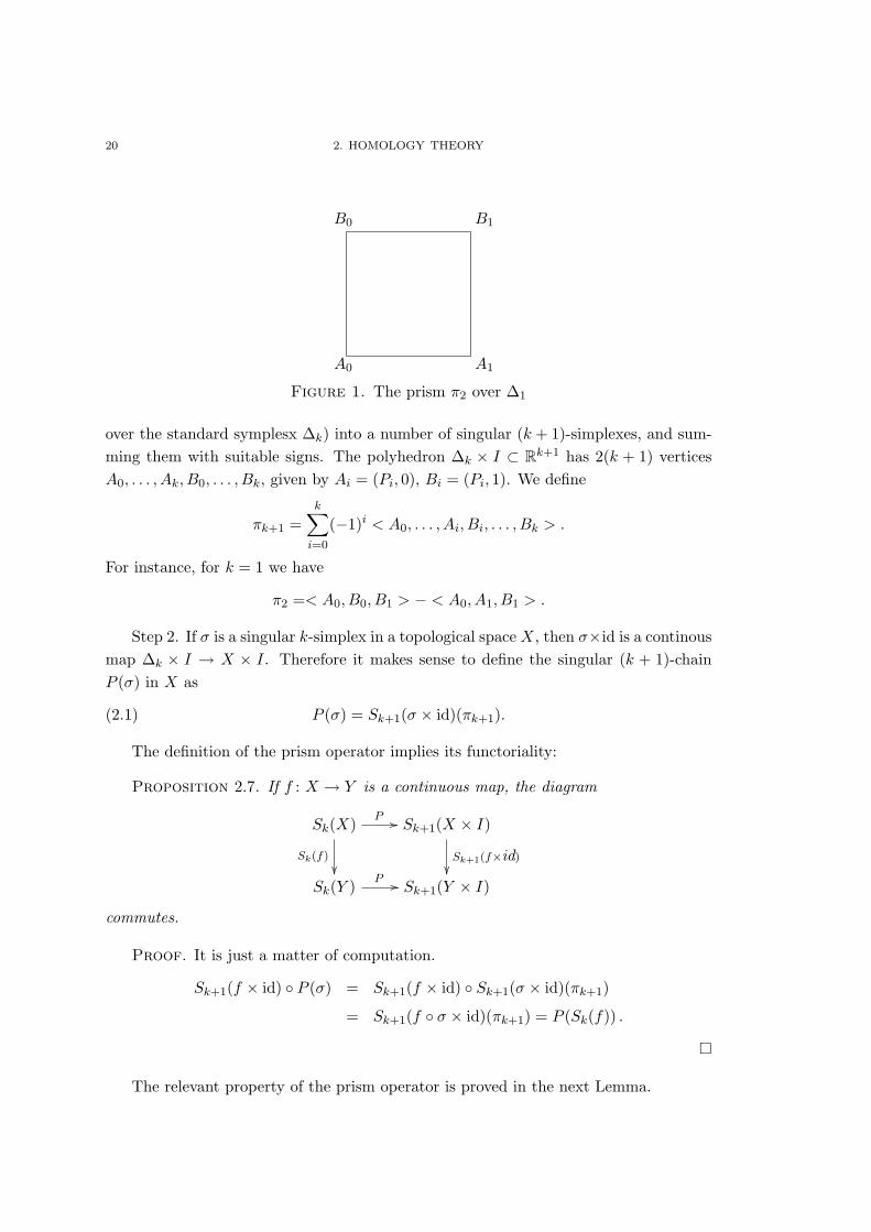
Figure 1. The prism π2 over ∆1
over the standard symplesx ∆k) into a number of singular (k + 1)-simplexes, and sum-ming them with suitable signs. The polyhedron ∆k × I ⊂ Rk+1 has 2(k + 1) verticesA0, . . . , Ak, B0, . . . , Bk, given by Ai = (Pi, 0), Bi = (Pi, 1). We define
πk+1 =k∑i=0
(−1)i < A0, . . . , Ai, Bi, . . . , Bk > .
For instance, for k = 1 we have
π2 =< A0, B0, B1 > − < A0, A1, B1 > .
Step 2. If σ is a singular k-simplex in a topological space X, then σ×id is a continousmap ∆k × I → X × I. Therefore it makes sense to define the singular (k + 1)-chainP (σ) in X as
(2.1) P (σ) = Sk+1(σ × id)(πk+1).
The definition of the prism operator implies its functoriality:
Proposition 2.7. If f : X → Y is a continuous map, the diagram
Sk(X) P //
Sk(f)
Sk+1(X × I)
Sk+1(f×id)
Sk(Y ) P // Sk+1(Y × I)
commutes.
Proof. It is just a matter of computation.
Sk+1(f × id) P (σ) = Sk+1(f × id) Sk+1(σ × id)(πk+1)
= Sk+1(f σ × id)(πk+1) = P (Sk(f)) .
The relevant property of the prism operator is proved in the next Lemma.
1. SINGULAR HOMOLOGY 21
Lemma 2.8. Let λ0, λi : X → X × I be the maps λ0(x) = (x, 0), λ1(x) = (x, 1).Then
(2.2) ∂ P + P ∂ = Sk(λ1)− Sk(λ0)
as maps Sk(X)→ Sk(X × I).
Proof. Let δk : ∆k → ∆k be the identity map regarded as singular k-simplex in∆k. Notice that P (δk) = πk+1.
We first check the identity (2.2) for X = ∆k, applying both sides of (2.2) to δk. Theright side yields
< B0, . . . , Bk > − < A0, . . . Ak > .
We compute now the action of the left side of (2.2) on δk.
∂P (δk) =k∑i=0
(−1)i∂ < A0, . . . , Ai, Bi, . . . , Bk >
=k∑
j≤i=0
(−1)i+j < A0, . . . , Aj , . . . Ai, Bi, . . . , Bk >
+k∑
i≤j=0
(−1)i+j+1 < A0, . . . Ai, Bi, . . . , Bj , . . . Bk > .
All terms with i = j cancel with the exception of < B0, . . . , Bk > − < A0, . . . Ak >. Sowe have
∂P (δk) = < B0, . . . , Bk > − < A0, . . . Ak >
+k∑
j<i=1
(−1)i+j < A0, . . . , Aj , . . . Ai, Bi, . . . , Bk >
−k∑
i<j=1
(−1)i+j < A0, . . . Ai, Bi, . . . , Bj , . . . Bk > .
On the other hand, one has
∂δk =k∑j=0
(−1)j < P0, . . . , Pj , . . . , Pk > .
Since
P (< P0, . . . , Pj , . . . , Pk >) =∑i<j
(−1)i < A0, . . . , Ai, Bi, . . . , Bj , . . . , Bk >
−∑i>j
(−1)i < A0, . . . , Aj , . . . , Ai, Bi, . . . , Bk >
we obtain the equation (2.2) (note that exchanging the indices i, j changes the sign).
22 2. HOMOLOGY THEORY
We must now prove that if equation (2.2) holds when both sides are applied to δk,then it holds in general. One has indeed
∂P (σ) = ∂Sk+1(σ × id)(P (δk)) = Sk(σ × id)(∂P (δk))
P (∂σ) = P∂(Sk(σ)(δk))
= P (Sk−1(σ)(∂δk)) = Sk(σ × id)(P (∂δk))
so that
∂P (σ) + P (∂σ) = Sk+1(σ × id)(∂P (δk)) + P (∂δk))
= Sk+1(σ × id)(Sk(λ1)− Sk(λ0)) = Sk(λ1)− Sk(λ0)
where λ0, λ1 are the obvious maps ∆k → ∆k × I.
Equation (2.2) states that P is a hotomopy (in the sense of homological algebra)between the maps λ0 and λ1, so that one has (λ1)[ = (λ2)[ in homology.
Proof of Proposition 2.5. Let F be a hotomopy between the maps f and g. Then,f = F λ0, g = F λ1, so that
f[ = (F λ0)[ = F[ (λ0)[ = F[ (λ1)[ = (F λ1)[ = g[.
Corollary 2.9. If X is a contractible space then
H0(X,R) ' R, Hk(X,R) = 0 for k > 0.
1.4. Relation between the first fundamental group and homology. A loopγ in X may be regarded as a closed singular 1-simplex. If we fix a point x0 ∈ X, wehave a set-theoretic map χ : L(x0) → S1(X,Z). The following result tells us that χdescends to a group homomorphism χ : π1(X,x0) → H1(X,Z).
Proposition 2.10. If two loops γ1, γ2 are homotopic, then they are homologousas singular 1-simplexes. Moreover, given two loops at x0, γ1, γ2, then χ(γ2 γ1) =χ(γ1) + χ(γ2) in H1(X,Z).
Proof. Choose a homotopy with fixed endpoints between γ1 and γ2, i.e., a mapΓ: I × I → X such that
Γ(t, 0) = γ1(t), Γ(t, 1) = γ2(t), Γ(0, s) = Γ(1, s) = x0 for all s ∈ I.
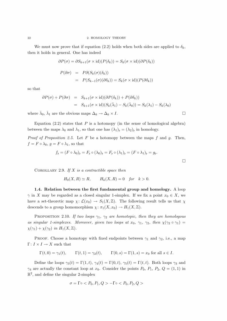
Define the loops γ3(t) = Γ(1, t), γ4(t) = Γ(0, t), γ5(t) = Γ(t, t). Both loops γ3 andγ4 are actually the constant loop at x0. Consider the points P0, P1, P2, Q = (1, 1) inR2, and define the singular 2-simplex
σ = Γ < P0, P1, Q > −Γ < P0, P2, Q >
1. SINGULAR HOMOLOGY 23
∧γ4 ∧ γ3
>γ2
>γ1
γ5
P0 P1
QP2
Figure 2
(cf. Figure 2). We then have
∂σ = Γ < P1, Q > −Γ < P0, Q > +Γ < P0, P1 >
− Γ < P2, Q > +Γ < P0, Q > −Γ < P0, P2 >
= γ3 − γ5 + γ1 − γ2 + γ5 + γ4 = γ1 − γ2.
This proves that χ(γ1) and χ(γ2) are homologous. To prove the second claim we needto define a singular 2-simplex σ such that
∂σ = γ1 + γ2 − γ2 · γ1.
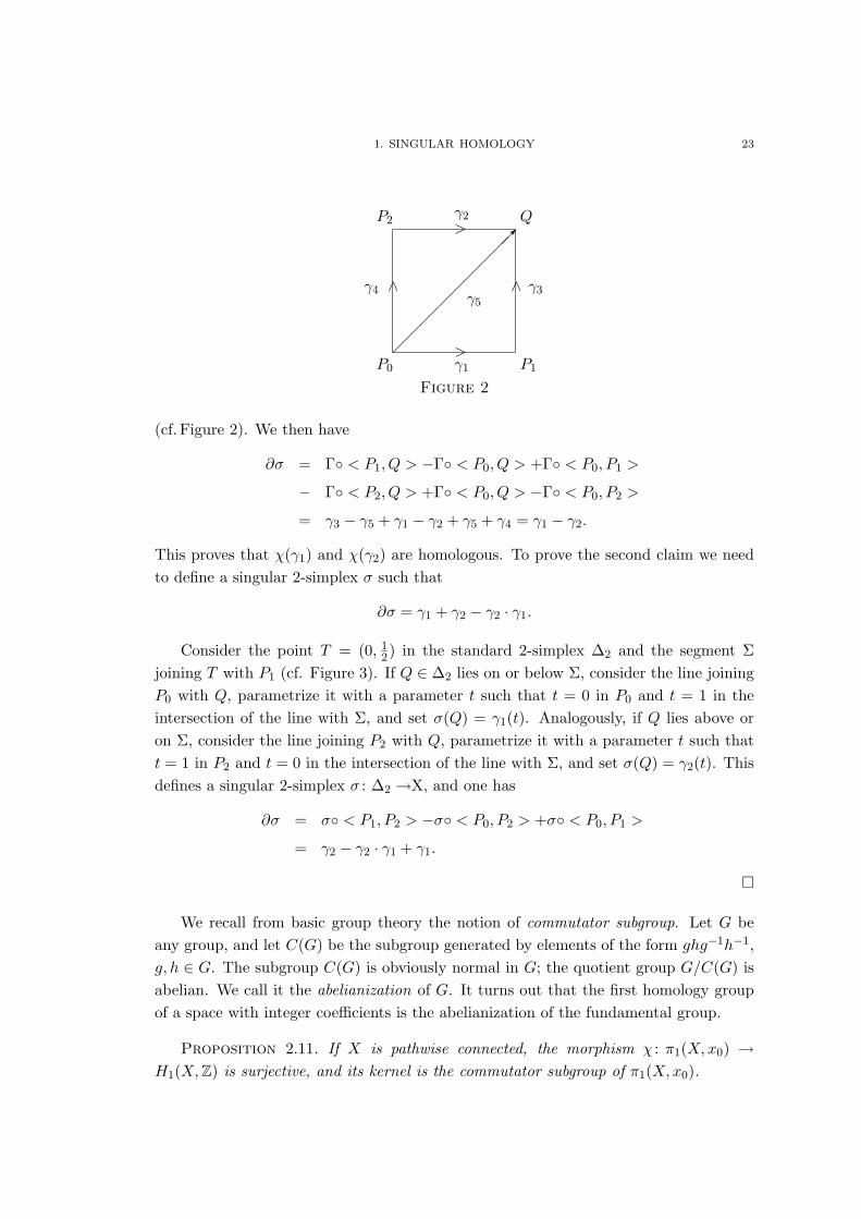
Consider the point T = (0, 12) in the standard 2-simplex ∆2 and the segment Σ
joining T with P1 (cf. Figure 3). If Q ∈ ∆2 lies on or below Σ, consider the line joiningP0 with Q, parametrize it with a parameter t such that t = 0 in P0 and t = 1 in theintersection of the line with Σ, and set σ(Q) = γ1(t). Analogously, if Q lies above oron Σ, consider the line joining P2 with Q, parametrize it with a parameter t such thatt = 1 in P2 and t = 0 in the intersection of the line with Σ, and set σ(Q) = γ2(t). Thisdefines a singular 2-simplex σ : ∆2 →X, and one has
∂σ = σ < P1, P2 > −σ < P0, P2 > +σ < P0, P1 >
= γ2 − γ2 · γ1 + γ1.
We recall from basic group theory the notion of commutator subgroup. Let G beany group, and let C(G) be the subgroup generated by elements of the form ghg−1h−1,g, h ∈ G. The subgroup C(G) is obviously normal in G; the quotient group G/C(G) isabelian. We call it the abelianization of G. It turns out that the first homology groupof a space with integer coefficients is the abelianization of the fundamental group.
Proposition 2.11. If X is pathwise connected, the morphism χ : π1(X,x0) →H1(X,Z) is surjective, and its kernel is the commutator subgroup of π1(X,x0).
24 2. HOMOLOGY THEORY
>
∧
∧
γ1
γ2
γ1
γ2
@@@@@@@@@@@@
HHHHHH
HHHHHH
AAAAAAAA
•Q
•Q
P0
P2
P1
T
Σ
Figure 3
Proof. Let c =∑
j ajσj be a 1-cycle. So we have
0 = ∂c =∑j
ai(σj(1)− σj(0)).
In this linear combination of points with coefficients in Z some of the points may coin-cide; the sum of the coefficients corresponding to the same point must vanish. Choose abase point x0 ∈ X and for every j choose a path αj from x0 to σj(0) and a path βj fromx0 to σj(1), in such a way that they depend on the endpoints and not on the indexing(e.g, if σj(0) = σk(0), choose αj = αk). Then we have∑
j
aj(βj − αj) = 0.
Now if we set σj = αj + σj − βj we have c =∑
j aj σj . Let γj be the loop β−1 · σj · α;then,
χ([Πjγ
ajj
]) = [c]
so that χ is surjective.
To prove the second claim we need to show that the commutator subgroup ofπ1(X,x0) coincides with kerχ. We first notice that since H1(X,Z) is abelian, thecommutator subgroup is necessarily contained in kerχ. To prove the opposite inclusion,let γ be a loop that in homology is a 1-boundary, i.e., γ = ∂
∑j ajσj . So we may write
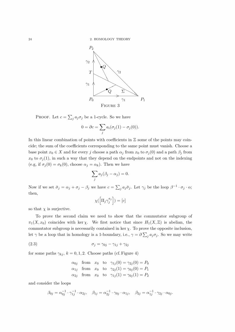
(2.3) σj = γ0j − γ1j + γ2j
for some paths γkj , k = 0, 1, 2. Choose paths (cf. Figure 4)
α0j from x0 to γ1j(0) = γ2j(0) = P0
α1j from x0 to γ2j(1) = γ0j(0) = P1
α2j from x0 to γ1j(1) = γ0j(1) = P2
and consider the loops
β0j = α−10j · γ
−11j · α2j , β1j = α−1
2j · γ0j · α1j , β2j = α−11j · γ2j · α0j .
2. RELATIVE HOMOLOGY 25
α1j
α0j
α2j
γ2j
γ0j γ1j
P1P0
P2
x0
Figure 4
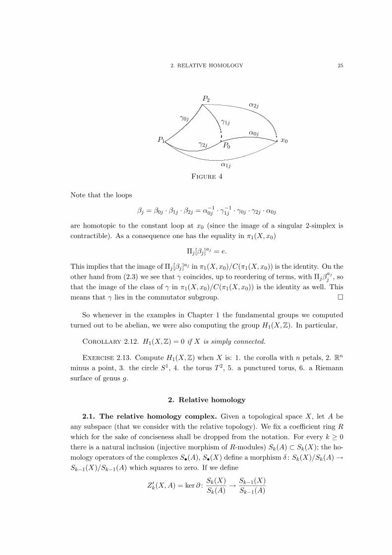
Note that the loops
βj = β0j · β1j · β2j = α−10j · γ
−11j · γ0j · γ2j · α0j
are homotopic to the constant loop at x0 (since the image of a singular 2-simplex iscontractible). As a consequence one has the equality in π1(X,x0)
Πj [βj ]aj = e.
This implies that the image of Πj [βj ]aj in π1(X,x0)/C(π1(X,x0)) is the identity. On theother hand from (2.3) we see that γ coincides, up to reordering of terms, with Πjβ
ajj , so
that the image of the class of γ in π1(X,x0)/C(π1(X,x0)) is the identity as well. Thismeans that γ lies in the commutator subgroup.
So whenever in the examples in Chapter 1 the fundamental groups we computedturned out to be abelian, we were also computing the group H1(X,Z). In particular,
Corollary 2.12. H1(X,Z) = 0 if X is simply connected.
Exercise 2.13. Compute H1(X,Z) when X is: 1. the corolla with n petals, 2. Rn
minus a point, 3. the circle S1, 4. the torus T 2, 5. a punctured torus, 6. a Riemannsurface of genus g.
2. Relative homology
2.1. The relative homology complex. Given a topological space X, let A beany subspace (that we consider with the relative topology). We fix a coefficient ring Rwhich for the sake of conciseness shall be dropped from the notation. For every k ≥ 0there is a natural inclusion (injective morphism of R-modules) Sk(A) ⊂ Sk(X); the ho-mology operators of the complexes S•(A), S•(X) define a morphism δ : Sk(X)/Sk(A)→Sk−1(X)/Sk−1(A) which squares to zero. If we define
Z ′k(X,A) = ker ∂ :Sk(X)Sk(A)
→ Sk−1(X)Sk−1(A)
26 2. HOMOLOGY THEORY
B′k(X,A) = Im ∂ :Sk+1(X)Sk+1(A)
→ Sk(X)Sk(A)
we have B′k(X,A) ⊂ Z ′k(X,A).
Definition 2.1. The homology groups of X relative to A are the R-modulesHk(X,A) = Z ′k(X,A)/B′k(X,A). When we want to emphasize the choice of the ring Rwe write Sk(X,A;R).
The relative homology is more conveniently defined in a slightly different way, whichmakes clearer its geometrical meaning. It will be useful to consider the following diagram
0
Zk(X)
qk //
Z ′k(X,A)
Sk(A) //
∂
Sk(X)qk //
∂
Sk(X)/Sk(A)
∂
// 0
0 // Bk−1(A) // Bk−1(X)qk−1
// B′k−1(X,A) // 0
Let
Zk(X,A) = c ∈ Sk(X) | ∂c ∈ Sk−1(A)
Bk(X,A) = c ∈ Sk(X) | c = ∂b+ c′ with b ∈ Sk+1(X), c′ ∈ Sk(A) .
Thus, Zk(X,A) is formed by the chains whose boundary is in A, and Bk(A) by thechains that are boundaries up to chains in A.
Lemma 2.2. Zk(X,A) is the pre-image of Z ′k(X,A) under the quotient homomor-phism qk; that is, an element c ∈ Sk(X) is in Zk(X,A) if and only if qk(c) ∈ Z ′k(X,A).
Proof. If qk(c) ∈ Z ′k(X,A) then 0 = ∂ qk(c) = qk−1 ∂(c) so that c ∈ Zk(X,A).If c ∈ Zk(X,A) then qk−1 ∂(c) = 0 so that qk(c) ∈ Z ′k(X,A).
Lemma 2.3. c ∈ Sk(X) is in Bk(X,A) if and only if qk(c) ∈ B′k(X,A).
Proof. If c = ∂b + c′ with b ∈ Sk+1(X) and c′ ∈ Sk(A) then qk(c) = qk ∂b =∂ qk+1(b) ∈ B′k(X,A). Conversely, if qk(c) ∈ B′k(X,A) then qk(c) = ∂ qk+1(b) forsome b ∈ Sk+1(X), then c− ∂b ∈ ker qk−1 so that c = ∂b+ c′ with c′ ∈ Sk(A).
Proposition 2.4. For all k ≥ 0, Hk(X,A) ' Zk(X,A)/Bk(X,A).
2. RELATIVE HOMOLOGY 27
Proof. What we should do is to prove the commutativity and the exactness of therows of the diagram
0 // Sk(A)
∼
// Bk(X,A)qk //
B′k(X,A)
// 0
0 // Sk(A) // Zk(X,A)qk // Z ′k(X,A) // 0
Commutativity is obvious. For the exactness of the first row, it is obvious that Sk(A) ⊂Bk(X,A) and that qk(c) = 0 if c ∈ Sk(A). On the other hand if c ∈ Bk(X,A) we havec = ∂b + c′ with b ∈ Sk+1(X) and c′ ∈ Sk(A), so that qk(c) = 0 implies 0 = qk ∂b =∂ qk+1(b), which in turn implies c ∈ Sk(A). To prove the surjectivity of qk, just noticethat by definition an element in B′k(X,A) may be represented as ∂b with b ∈ Sk+1(X).
As for the second row, we have Sk(A) ⊂ Zk(X,A) from the definition of Zk(X,A).If c ∈ Sk(A) then qk(c) = 0. If c ∈ Zk(X,A) and qk(c) = 0 then c ∈ Sk(A) by thedefinition of Z ′k(X,A). Moreover qk is surjective by Lemma 2.2.
2.2. Main properties of relative homology. We list here the main propertiesof the cohomology groups Hk(X,A). If a proof is not given the reader should provideone by her/himself.
• If A is empty, Hk(X,A) ' Hk(X).
• The relative cohomology groups are functorial in the following sense. Given topo-logical spaces X, Y with subsets A ⊂ X, B ⊂ Y , a continous map of pairs is a con-tinuous map f : X → Y such that f(A) ⊂ B. Such a map induces in natural way amorphisms of R-modules f[ : H•(X,A)→ H•(Y,B). If we consider the inclusion of pairs(X, ∅) → (X,A) we obtain a morphism H•(X)→• H(X,A).
• The inclusion map i : A → X induces a morphism H•(A) → H•(X) and thecomposition H•(A)→ H•(X)→ H•(X,A) vanishes (since Zk(A) ⊂ Bk(X,A)).
• If X = ∪jXj is a union of pathwise connected components, then Hk(X,A) '⊕jHk(Xj , Aj) where Aj = A ∩Xj .
Proposition 2.5. If X is pathwise connected and A is nonempty, then H0(X,A)= 0.
Proof. If c =∑
j ajxj ∈ S0(X) and γj is a path from x0 ∈ A to xj , then∂(∑
j ajxj) = c− (∑
j aj)x0 so that c ∈ B0(X,A).
Corollary 2.6. H0(X,A) is a free R-module generated by the components of Xthat do not meet A.
Indeed Hj(Xj , Aj) = 0 if Aj is empty.
Proposition 2.7. If A = x0 is a point, Hk(X,A) ' Hk(X) for k > 0.
28 2. HOMOLOGY THEORY
Proof.
Zk(X,A) = c ∈ Sk(X) | ∂c ∈ Sk−1(A) = Zk(X) when k > 0
Bk(X,A) = c ∈ Sk(X) | c = ∂b+ c′ with b ∈ Sk+1(X), c′ ∈ Sk(A)= Bk(X) when k > 0.
2.3. The long exact sequence of relative homology. By definition the relativehomology of X with respect to A is the homology of the quotient complex S•(X)/S•(A).By Proposition 1.7, adapted to homology by reversing the arrows, one obtains a longexact cohomology sequence
· · · → H2(A)→ H2(X)→ H2(X,A)
→ H1(A)→ H1(X)→ H1(X,A)
→ H0(A)→ H0(X)→ H0(X,A)→ 0
Exercise 2.8. Assume to know that H1(S1, R) ' R and Hk(S1, R) = 0 for k >1. Use the long relative homology sequence to compute the relative homology groupsH•(R2, S1;R).
3. The Mayer-Vietoris sequence
The Mayer-Vietoris sequence (in its simplest form, that we are going to considerhere) allows one to compute the homology of a union X = U ∪ V from the knowledgeof the homology of U , V and U ∩ V . This is quite similar to what happens in de Rhamcohomology, but in the case of homology there is a subtlety. Let us denote A = U ∩ V .One would think that there is an exact sequence
0→ Sk(A) i→ Sk(U)⊕ Sk(V )p→ Sk(X)→ 0
where i is the morphism induced by the inclusions A → U , A → V , and p is given byp(σ1, σ2) = σ1 − σ2 (again using the inclusions U → X, V → X). However, it is notpossible to prove that p is surjective (if σ is a singular k-simplex whose image is notcontained in U or V , it is not in general possible to write it as a difference of standardk-simplexes in U , V ). The trick to circumvent this difficulty consists in replacing S•(X)with a different complex that however has the same homology.
Let U = Uα be an open cover of X.
Definition 2.1. A singular k-chain σ =∑
j ajσj is U-small if every singular k-simplex σj maps into an open set Uα ∈ U for some α. Moreover we define SU
• (X) asthe subcomplex of S•(X) formed by U-small chains.1
The homology differential ∂ restricts to SU• (X), so that one has a homology HU
• (X).
1Again, we understand the choice of a coefficient ring R.
3. THE MAYER-VIETORIS SEQUENCE 29
HHHHHH
B
E0
E1
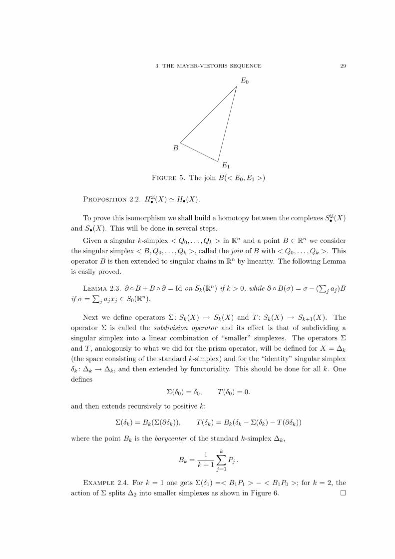
Figure 5. The join B(< E0, E1 >)
Proposition 2.2. HU• (X) ' H•(X).
To prove this isomorphism we shall build a homotopy between the complexes SU• (X)
and S•(X). This will be done in several steps.
Given a singular k-simplex < Q0, . . . , Qk > in Rn and a point B ∈ Rn we considerthe singular simplex < B,Q0, . . . , Qk >, called the join of B with < Q0, . . . , Qk >. Thisoperator B is then extended to singular chains in Rn by linearity. The following Lemmais easily proved.
Lemma 2.3. ∂ B +B ∂ = Id on Sk(Rn) if k > 0, while ∂ B(σ) = σ− (∑
j aj)Bif σ =
∑j ajxj ∈ S0(Rn).
Next we define operators Σ: Sk(X) → Sk(X) and T : Sk(X) → Sk+1(X). Theoperator Σ is called the subdivision operator and its effect is that of subdividing asingular simplex into a linear combination of “smaller” simplexes. The operators Σand T , analogously to what we did for the prism operator, will be defined for X = ∆k
(the space consisting of the standard k-simplex) and for the “identity” singular simplexδk : ∆k → ∆k, and then extended by functoriality. This should be done for all k. Onedefines
Σ(δ0) = δ0, T (δ0) = 0.
and then extends recursively to positive k:
Σ(δk) = Bk(Σ(∂δk)), T (δk) = Bk(δk − Σ(δk)− T (∂δk))
where the point Bk is the barycenter of the standard k-simplex ∆k,
Bk =1
k + 1
k∑j=0
Pj .
Example 2.4. For k = 1 one gets Σ(δ1) =< B1P1 > − < B1P0 >; for k = 2, theaction of Σ splits ∆2 into smaller simplexes as shown in Figure 6.
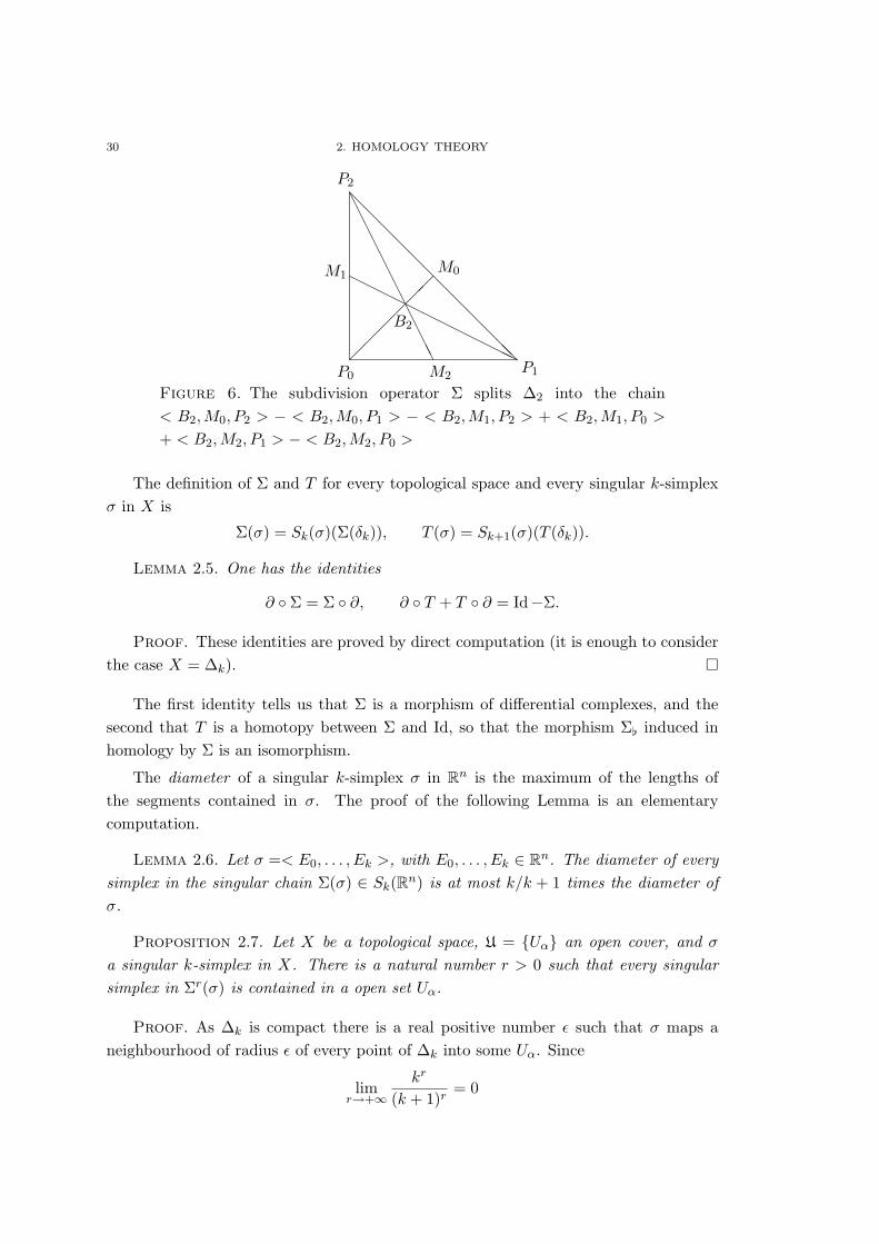
30 2. HOMOLOGY THEORY
@@@@@@@@@@@@
HHHHHH
HHHHHH
AAAAAAAAAAAA
B2
P0P1
P2
M1
M2
M0
Figure 6. The subdivision operator Σ splits ∆2 into the chain< B2,M0, P2 > − < B2,M0, P1 > − < B2,M1, P2 > + < B2,M1, P0 >
+ < B2,M2, P1 > − < B2,M2, P0 >
The definition of Σ and T for every topological space and every singular k-simplexσ in X is
Σ(σ) = Sk(σ)(Σ(δk)), T (σ) = Sk+1(σ)(T (δk)).
Lemma 2.5. One has the identities
∂ Σ = Σ ∂, ∂ T + T ∂ = Id−Σ.
Proof. These identities are proved by direct computation (it is enough to considerthe case X = ∆k).
The first identity tells us that Σ is a morphism of differential complexes, and thesecond that T is a homotopy between Σ and Id, so that the morphism Σ[ induced inhomology by Σ is an isomorphism.
The diameter of a singular k-simplex σ in Rn is the maximum of the lengths ofthe segments contained in σ. The proof of the following Lemma is an elementarycomputation.
Lemma 2.6. Let σ =< E0, . . . , Ek >, with E0, . . . , Ek ∈ Rn. The diameter of everysimplex in the singular chain Σ(σ) ∈ Sk(Rn) is at most k/k + 1 times the diameter ofσ.
Proposition 2.7. Let X be a topological space, U = Uα an open cover, and σ
a singular k-simplex in X. There is a natural number r > 0 such that every singularsimplex in Σr(σ) is contained in a open set Uα.
Proof. As ∆k is compact there is a real positive number ε such that σ maps aneighbourhood of radius ε of every point of ∆k into some Uα. Since
limr→+∞
kr
(k + 1)r= 0
3. THE MAYER-VIETORIS SEQUENCE 31
there is an r > 0 such that Σr(δk) is a linear combination of simplexes whose diameteris less than ε. But as Σr(σ) = Sk(σ)(Σr(δk)) we are done.
This completes the proof of Proposition 2.2. We may now prove the exactness ofthe Mayer-Vietoris sequence in the following sense. If X = U ∪ V (union of two opensubsets), let U = U, V and A = U ∩ V .
Proposition 2.8. For every k there is an exact sequence of R-modules
0→ Sk(A) i→ Sk(U)⊕ Sk(V )p→ SU
k (X)→ 0 .
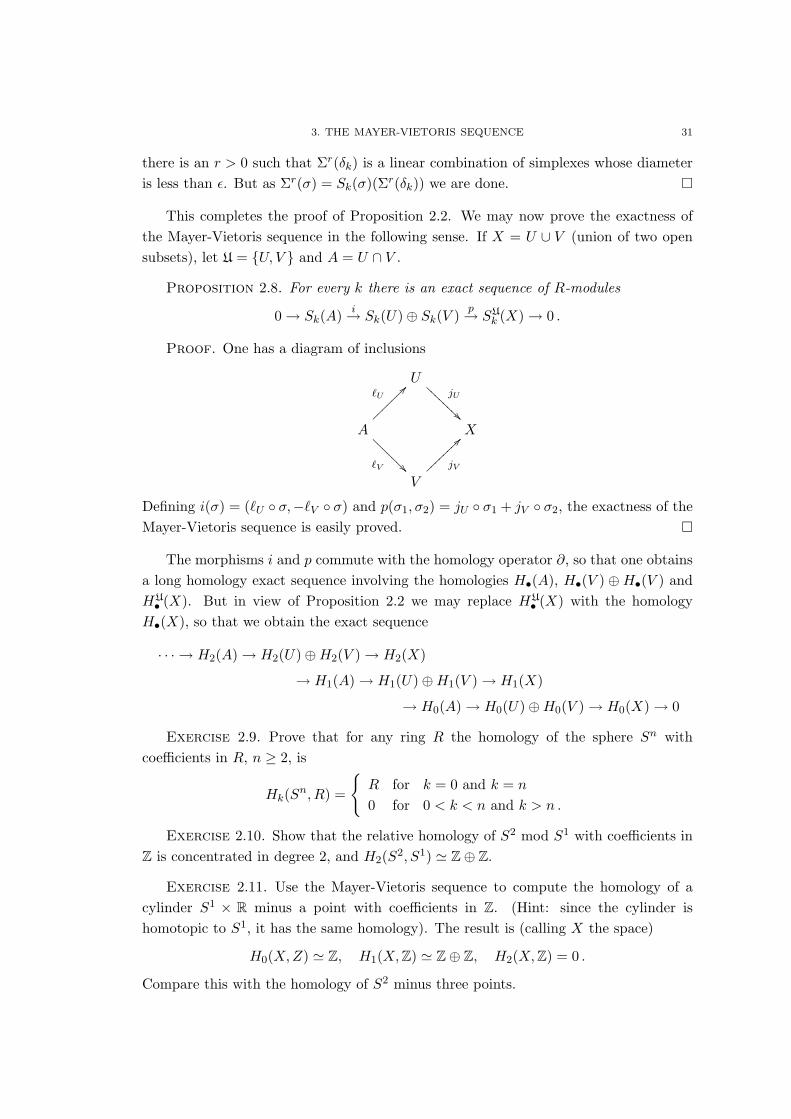
Proof. One has a diagram of inclusions
UjU
@@@
@@@@
@
A
`U??~~~~~~~
`V @@@
@@@@
X
V
jV
>>~~~~~~~~
Defining i(σ) = (`U σ,−`V σ) and p(σ1, σ2) = jU σ1 + jV σ2, the exactness of theMayer-Vietoris sequence is easily proved.
The morphisms i and p commute with the homology operator ∂, so that one obtainsa long homology exact sequence involving the homologies H•(A), H•(V ) ⊕H•(V ) andHU• (X). But in view of Proposition 2.2 we may replace HU
• (X) with the homologyH•(X), so that we obtain the exact sequence
· · · → H2(A)→ H2(U)⊕H2(V )→ H2(X)
→ H1(A)→ H1(U)⊕H1(V )→ H1(X)
→ H0(A)→ H0(U)⊕H0(V )→ H0(X)→ 0
Exercise 2.9. Prove that for any ring R the homology of the sphere Sn withcoefficients in R, n ≥ 2, is
Hk(Sn, R) =
R for k = 0 and k = n
0 for 0 < k < n and k > n .
Exercise 2.10. Show that the relative homology of S2 mod S1 with coefficients inZ is concentrated in degree 2, and H2(S2, S1) ' Z⊕ Z.
Exercise 2.11. Use the Mayer-Vietoris sequence to compute the homology of acylinder S1 × R minus a point with coefficients in Z. (Hint: since the cylinder ishomotopic to S1, it has the same homology). The result is (calling X the space)
H0(X,Z) ' Z, H1(X,Z) ' Z⊕ Z, H2(X,Z) = 0 .
Compare this with the homology of S2 minus three points.
32 2. HOMOLOGY THEORY
4. Excision
If a space X is the union of subspaces, the Mayer-Vietoris suquence allows one tocompute the homology of X from the homology of the subspaces and of their intersec-tions. The operation of excision in some sense gives us information about the reverseoperation, i.e., it tells us what happen to the homology of a space if we “excise” a sub-pace out of it. Let us recall that given a map f : (X,A)→ (Y,B) (i.e., a map f : X → Y
such that f(A) ⊂ B) there is natural morphism f[ : H•(X,A)→ H•(Y,B).
Definition 2.1. Given nested subspaces U ⊂ A ⊂ X, the inclusion map (X−U,A−U) → (X,A) is said to be an excision if the induced morphism Hk(X − U,A − U) →Hk(X,A) is an isomorphism for all k.
If (X − U,A− U)→ (X,A) is an excision, we say that U “can be excised.”
To state the main theorem about excision we need some definitions from topology.
Definition 2.2. 1. Let i : A → X be an inclusion of topological spaces. A mapr : X → A is a retraction of i if r i = IdA.
2. A subspace A ⊂ X is a deformation retract of X if IdX is homotopically equivalentto i r, where r : X → A is a retraction.
If r : X → A is a retraction of i : A→ X, then r[ i[ = IdH•(A), so that i[ : H•(A)→H•(X) is injective. Moreover, if A is a deformation retract of X, then H•(A) ' H•(X).The same notion can be given for inclusions of pairs, (A,B) → (X,Y ); if such a map isa deformation retract, then H•(A,B) ' H•(X,Y ).
Exercise 2.3. Show that no retraction Sn → Sn−1 can exist.
Theorem 2.4. If the closure U of U lies in the interior int(A) of A, then U can beexcised.
Proof. We consider the cover U = X − U, int(A) of X. Let c =∑
j ajσj ∈Zk(X,A), so that ∂c ∈ Sk−1(A). In view of Proposition 2.2 we may assume that c is U-small. If we cancel from σ those singular simplexes σj taking values in int(A), the class[c] ∈ Hk(X,A) is unchanged. Therefore, after the removal, we can regard c as a relativecycle in X−U mod A−U ; this implies that the morphism Hk(X−U,A−U)→ Hk(X,A)is surjective.
To prove that it is injective, let [c] ∈ Hk(X −U,A−U) be such that, regarding c asa cycle in X mod A, it is a boundary, i.e., c ∈ Bk(X,A). This means that
c = ∂b+ c′ with b ∈ Sk+1(X), c′ ∈ Sk(A) .
We apply the operator Σr to both sides of this inequality, and split Σr(b) into b1 + b2,where b1 maps into X − U and b2 into int(A). We have
Σr(c)− ∂b1 = Σr(c′) + ∂b2 .
4. EXCISION 33
The chain in the left side is in X−U while the chain in the right side is in A; therefore,both chains are in (X − U) ∩A = A− U . Now we have
Σr(c) = Σr(c′) + ∂b2 + ∂b1
with Σr(c′)+∂b2 ∈ Sk(A−U) and ∂b1 ∈ Sk+1(X−U) so that Σr(c) ∈ Bk(X−U,A−U),which implies [c] = 0 (in Hk(X − U,A− U)).
Exercise 2.5. Let B an open band around the equator of S2, and x0 ∈ B. Computethe relative homology H•(S2 − x0, B − x0; Z).
To describe some more applications of excision we need the notion of augmentedhomology modules. Given a topological space X and a ring R, let us define
∂] : S0(X,R) → R∑j
ajσj 7→∑j
aj .
We define the augmented homology modules
H]0(X,R) = ker ∂]/B0(X,R) , H]
k(X,R) = Hk(X,R) for k > 0 .
If A ⊂ X, one defines the augmented relative homology modules H]k(X,A;R) in a
similar way, i.e.,
H]k(X,A;R) = Hk(X,A;R) if A 6= ∅, H]
k(X,A;R) = Hk(X,R) if A = ∅ .
Exercise 2.6. Prove that there is a long exact sequence for the augmented relativehomology modules.
Exercise 2.7. Let Bn be the closed unit ball in Rn+1, Sn its boundary, and let E±nbe the two closed (northern, southern) emispheres in Sn.
1. Use the long exact sequence for the augmented relative homology modules toprove that H]
k(Sn) ' H]
k(Sn, E−n ) and H]
k−1(Sn−1) ' H]k(B
n, Sn−1). So we haveH]k(B
n, Sn−1) = 0 for k < n, H]n(Bn, Sn−1) ' R
2. Use excision to show that H]k(S
n, E−n ) ' H]k(B
n, Sn−1).
3. Deduce that H]k(S
n) ' H]k−1(Sn−1).
Exercise 2.8. Let Sn be the sphere realized as the unit sphere in Rn+1, and letr : Sn → Sn → Sn be the reflection
r(x0, x1, . . . , xn) = (−x0, x1, . . . , xn).
34 2. HOMOLOGY THEORY
Prove that r[ : Hn(Sn)→ Hn(Sn) is the multiplication by −1. (Hint: this is trivial forn = 0, and can be extended by induction using the commutativity of the diagram
Hn(Sn) ∼ //
r[
H]n−1(Sn−1)
r[
Hn(Sn) ∼ // H]n−1(Sn−1)
which follows from Exercise 2.7.
Exercise 2.9. 1. The rotation group O(n + 1) acts on Sn. Show that for anyM ∈ O(n + 1) the induced morphism M[ : Hn(Sn) → Hn(Sn) is the multiplication bydetM = ±1.
2. Let a : Sn → Sn be the antipodal map, a(x) = −x. Show that a[ : Hn(Sn) →Hn(Sn) is the multiplication by (−1)n+1.
Example 2.10. We show that the inclusion map (E+n , S
n−1) → (Sn, E−n ) is anexcision. (Here we are excising the open southern emisphere, i.e., with reference to thegeneral theory, X = Sn, U = the open southern emisphere, A = E−n .)
The hypotheses of Theorem 2.4 are not satisfied. However it is enough to considerthe subspace
V =x ∈ Sn |x0 > −1
2
.
V can be excised from (Sn, E−n ). But (E+n , S
n−1) is a deformation retract of (Sn −V,E−n − V ) so that we are done.
We end with a standard application of algebraic topology. Let us define a vectorfield on Sn as a continous map v : Sn → Rn+1 such that v(x) · x = 0 for all x ∈ Sn (theproduct is the standard scalar product in Rn+1).
Proposition 2.11. A nowhere vanishing vector field v on Sn exists if and only ifn is odd.
Proof. If n = 2m+ 1 a nowhere vanishing vector field is given by
v(x0, . . . , x2m+1) = (−x1, x0,−x3, x2, . . . ,−x2m+1, x2m) .
Conversely, assume that such a vector field exists. Define
w(x) =v(x)‖v(x)‖
;
this is a map Sn → Sn, with w(x) · x = 0 for all x ∈ Sn. Define
F : Sn × I → Sn
F (x, t) = x cos tπ + w(x) sin tπ.
SinceF (x, 0) = x, F (x, 1
2) = w(x), F (x, 1) = −x
4. EXCISION 35
the three maps Id, w, a are homotopic. But as a consequence of Exercise 2.9, n mustbe odd.

CHAPTER 3
Introduction to sheaves and their cohomology
1. Presheaves and sheaves
Let X be a topological space.
Definition 3.1. A presheaf of Abelian groups on X is a rule1 P which assigns anAbelian group P(U) to each open subset U of X and a morphism (called restriction map)ϕU,V : P(U) → P(V ) to each pair V ⊂ U of open subsets, so as to verify the followingrequirements:
(1) P(∅) = 0;(2) ϕU,U is the identity map;
(3) if W ⊂ V ⊂ U are open sets, then ϕU,W = ϕV,W ϕU,V .
The elements s ∈ P(U) are called sections of the presheaf P on U . If s ∈ P(U) isa section of P on U and V ⊂ U , we shall write s|V instead of ϕU,V (s). The restrictionP|U of P to an open subset U is defined in the obvious way.
Presheaves of rings are defined in the same way, by requiring that the restrictionmaps are ring morphisms. If R is a presheaf of rings on X, a presheaf M of Abeliangroups on X is called a presheaf of modules over R (or an R-module) if, for each opensubset U , M(U) is an R(U)-module and for each pair V ⊂ U the restriction mapϕU,V : M(U) → M(V ) is a morphism of R(U)-modules (where M(V ) is regarded asan R(U)-module via the restriction morphism R(U) → R(V )). The definitions in thisSection are stated for the case of presheaves of Abelian groups, but analogous definitionsand properties hold for presheaves of rings and modules.
Definition 3.2. A morphism f : P → Q of presheaves over X is a family of mor-phisms of Abelian groups fU : P(U)→ Q(U) for each open U ⊂ X, commuting with the
1This rather naive terminology can be made more precise by saying that a presheaf on X is a
contravariant functor from the category OX of open subsets of X to the category of Abelian groups.
OX is defined as the category whose objects are the open subsets of X while the morphisms are the
inclusions of open sets.
37
38 3. SHEAVES AND THEIR COHOMOLOGY
restriction morphisms; i.e., the following diagram commutes:
P(U)fU−−−−→ Q(U)
ϕU,V
y yϕU,VP(V )
fV−−−−→ Q(V )
Definition 3.3. The stalk of a presheaf P at a point x ∈ X is the Abelian group
Px = lim−→U
P(U)
where U ranges over all open neighbourhoods of x, directed by inclusion.
Remark 3.4. We recall here the notion of direct limit. A directed set I is a partiallyordered set such that for each pair of elements i, j ∈ I there is a third element k suchthat i < k and j < k. If I is a directed set, a directed system of Abelian groups isa family Gii∈I of Abelian groups, such that for all i < j there is a group morphismfij : Gi → Gj , with fii = id and fij fjk = fik. On the set G =
∐i∈I Gi, where
∐denotes disjoint union, we put the following equivalence relation: g ∼ h, with g ∈ Giand h ∈ Gj , if there exists a k ∈ I such that fik(g) = fjk(h). The direct limit l of thesystem Gii∈I , denoted l = lim−→i∈I Gi, is the quotient G/ ∼. Heuristically, two elementsin G represent the same element in the direct limit if they are ‘eventually equal.’ Fromthis definition one naturally obtains the existence of canonical morphisms Gi → l. Thefollowing discussion should make this notion clearer; for more detail, the reader mayconsult [13].
If x ∈ U and s ∈ P(U), the image sx of s in Px via the canonical projectionP(U)→ Px (see footnote) is called the germ of s at x. From the very definition of directlimit we see that two elements s ∈ P(U), s′ ∈ P(V ), U , V being open neighbourhoodsof x, define the same germ at x, i.e. sx = s′x, if and only if there exists an openneighbourhood W ⊂ U ∩ V of x such that s and s′ coincide on W , s|W = s′|W .
Definition 3.5. A sheaf on a topological space X is a presheaf F on X which fulfillsthe following axioms for any open subset U of X and any cover Ui of U .
S1) If two sections s ∈ F(U), s ∈ F(U) coincide when restricted to any Ui, s|Ui =s|Ui, they are equal, s = s.
S2) Given sections si ∈ F(Ui) which coincide on the intersections, si|Ui∩Uj =sj |Ui∩Uj for every i, j, there exists a section s ∈ F(U) whose restriction toeach Ui equals si, i.e. s|Ui = si.
Thus, roughly speaking, sheaves are presheaves defined by local conditions. Thestalk of a sheaf is defined as in the case of a presheaf.
1. PRESHEAVES AND SHEAVES 39
Example 3.6. If F is a sheaf, and Fx = 0 for all x ∈ X, then F is the zero sheaf,F(U) = 0 for all open sets U ⊂ X. Indeed, if s ∈ F(U), since sx = 0 for all x ∈ U ,there is for each x ∈ U an open neighbourhood Ux such that s|Ux = 0. The first sheafaxiom then implies s = 0. This is not true for a presheaf, cf. Example 3.15 below.
A morphism of sheaves is just a morphism of presheaves. If f : F → G is a morphismof sheaves onX, for every x ∈ X the morphism f induces a morphism between the stalks,fx : Fx → Gx, in the following way: since the stalk Fx is the direct limit of the groupsF(U) over all open U containing x, any g ∈ Fx is of the form g = sx for some openU 3 x and some s ∈ F(U); then set fx(g) = (fU (s))x.
A sequence of morphisms of sheaves 0 → F ′ → F → F ′′ → 0 is exact if for everypoint x ∈ X, the sequence of morphisms between the stalks 0 → F ′x → Fx → F ′′x → 0is exact. If 0 → F ′ → F → F ′′ → 0 is an exact sequence of sheaves, for every opensubset U ⊂ X the sequence of groups 0 → F ′(U) → F(U) → F ′′(U) is exact, but thelast arrow may fail to be surjective. Instances of this situation are shown in Examples3.11 and 3.12 below.
Exercise 3.7. Let 0→ F ′ → F → F ′′ → 0 be an exact sequence of sheaves. Showthat 0→ F ′ → F → F ′′ is an exact sequence of presheaves.
Example 3.8. Let G be an Abelian group. Defining P(U) ≡ G for every opensubset U and taking the identity maps as restriction morphisms, we obtain a presheaf,called the constant presheaf GX . All stalks (GX)x of GX are isomorphic to the groupG. The presheaf GX is not a sheaf: if V1 and V2 are disjoint open subsets of X, andU = V1 ∪V2, the sections g1 ∈ GX(V1) = G, g2 ∈ GX(V2) = G, with g1 6= g2, satisfy thehypothesis of the second sheaf axiom S2) (since V1 ∩V2 = ∅ there is nothing to satisfy),but there is no section g ∈ GX(U) = G which restricts to g1 on V1 and to g2 on V2.
Example 3.9. Let CX(U) be the ring of real-valued continuous functions on an openset U of X. Then CX is a sheaf (with the obvious restriction morphisms), the sheaf ofcontinuous functions on X. The stalk Cx ≡ (CX)x at x is the ring of germs of continuousfunctions at x.
Example 3.10. In the same way one can define the following sheaves:
The sheaf C∞X of differentiable functions on a differentiable manifold X.
The sheaves ΩpX of differential p-forms, and all the sheaves of tensor fields on a
differentiable manifold X.
The sheaf of holomorphic functions on a complex manifold and the sheaves of holo-morphic p-forms on it.
The sheaves of forms of type (p, q) on a complex manifold X.
Example 3.11. Let X be a differentiable manifold, and let d : Ω•X → Ω•X be theexterior differential. We can define the presheaves ZpX of closed differential p-forms, and
40 3. SHEAVES AND THEIR COHOMOLOGY
BpX of exact p-differential forms,
ZpX(U) = ω ∈ ΩpX(U) | dω = 0,
BpX(U) = ω ∈ ΩpX(U) |ω = dτ for some τ ∈ Ωp−1
X (U).ZpX is a sheaf, since the condition of being closed is local: a differential form is closed ifand only if it is closed in a neighbourhood of each point of X. On the contrary, BpX isnot a sheaf. In fact, if X = R2, the presheaf B1
X of exact differential 1-forms does notfulfill the second sheaf axiom: consider the form
ω =xdy − ydxx2 + y2
defined on the open subset U = X − (0, 0). Since ω is closed on U , there is anopen cover Ui of U by open subsets where ω is an exact form, ω|Ui ∈ B1
X(Ui) (this isPoincare’s lemma). But ω is not an exact form on U because its integral along the unitcircle is different from 0.
This means that, while the sequence of sheaf morphisms 0→ R→ C∞Xd−−→Z1
X → 0
is exact (Poincare lemma), the morphism C∞X (U) d−−→Z1X(U) may fail to be surjective.
Example 3.12. Let X be a complex manifold, Z the constant sheaf with stalk theintegers, O the sheaf of holomorphic functions on X, and O∗ the sheaf of nowherevanishing holomorphic functions. In analogy with the exact sequence (1.1) we mayconsider the sequence
(3.1) 0→ Z→ O exp−−→O∗ → 1
This is an exact sequence of sheaves, in particular exp: C → C∗ is surjective as a mapof sheaves, since in a neighbourhood of every point, an inverse my be found by applyingthe logarithm function. However, since the latter is multi-valued, surjectivity fails onnon-simply connected open sets. See Example 3.11.
1.1. Etale space. We wish now to describe how, given a presheaf, one can natu-rally associate with it a sheaf having the same stalks. As a first step we consider the caseof a constant presheaf GX on a topological space X, where G is an Abelian group. Wecan define another presheaf GX on X by putting GX(U) = locally constant functionsf : U → G, 2 where GX(U) = G is included as the constant functions. It is clear that(GX)x = Gx = G at each point x ∈ X and that GX is a sheaf, called the constant sheafwith stalk G. Notice that the functions f : U → G are the sections of the projectionπ :∐x∈X Gx → X and the locally constant functions correspond to those sections which
locally coincide with the sections produced by the elements of G.
Now, let P be an arbitrary presheaf on X. Consider the disjoint union of the stalksP =
∐x∈X Px and the natural projection π : P → X. The sections s ∈ P(U) of the
2A function is locally constant on U if it is constant on any connected component of U .
1. PRESHEAVES AND SHEAVES 41
presheaf P on an open subset U produce sections s : U → P of π, defined by s(x) = sx,and we can define a new presheaf P\ by taking P\(U) as the group of those sectionsσ : U → P of π such that for every point x ∈ U there is an open neighbourhood V ⊂ Uof x which satisfies σ|V = s for some s ∈ P(V ).
That is, P\ is the presheaf of all sections that locally coincide with sections of P. Itcan be described in another way by the following construction.
Definition 3.13. The set P, endowed with the topology whose base of open subsetsconsists of the sets s(U) for U open in X and s ∈ P(U), is called the etale space of thepresheaf P.
Exercise 3.14. (1) Show that π : P → X is a local homeomorphism, i.e., everypoint u ∈ P has an open neighbourhood U such that π : U → π(U) is ahomeomorphism.
(2) Show that for every open set U ⊂ X and every s ∈ P(U), the section s : U → Pis continuous.
(3) Prove that P\ is the sheaf of continuous sections of π : P → X.(4) Prove that for all x ∈ X the stalks of P and P\ at x are isomorphic.(5) Show that there is a presheaf morphism φ : P → P\.(6) Show that φ is an isomorphism if and only if P is a sheaf.
P\ is called the sheaf associated with the presheaf P. In general, the morphismφ : P → P\ is neither injective nor surjective: for instance, the morphism between theconstant presheaf GX and its associated sheaf GX is injective but nor surjective.
Example 3.15. As a second example we study the sheaf associated with the presheafBkX of exact k-forms on a differentiable manifold X. For any open set U we have anexact sequence of Abelian groups (actually of R-vector spaces)
0→ BkX(U)→ ZkX(U)→ HkX(U)→ 0
where HkX is the presheaf that with any open set U associates its k-th de Rham coho-mology group, HkX(U) = Hk
DR(U). Now, the open neighbourhoods of any point x ∈ Xwhich are diffeomorphic to Rn (where n = dimX) are cofinal3 in the family of all openneighbourhoods of x, so that (HkX)x = 0 by the Poincare lemma. In accordance withExample 3.6 this means that (HkX)\ = 0, which is tantamount to (BkX)\ ' ZkX .
In this case the natural morhism HkX → (HkX)\ is of course surjective but notinjective. On the other hand, BkX → (BkX)\ = ZkX is injective but not surjective.
3Let I be a directed set. A subset J of I is said to be cofinal if for any i ∈ I there is a j ∈ J
such that i < j. By the definition of direct limit we see that, given a directed family of Abelian groups
Gii∈I , if Gjj∈J is the subfamily indexed by J , then
lim−→i∈I
Gi ' lim−→j∈J
Gj ;
that is, direct limits can be taken over cofinal subsets of the index set.
42 3. SHEAVES AND THEIR COHOMOLOGY
Definition 3.16. Given a sheaf F on a topological space X and a subset (notnecessarily open) S ⊂ X, the sections of the sheaf F on S are the continuous sectionsσ : S → F of π : F → X. The group of such sections is denoted by Γ(S, F).
Definition 3.17. Let P, Q be presheaves on a topological space X. 4
(1) The direct sum of P and Q is the presheaf P ⊕ Q given, for every open subsetU ⊂ X, by (P ⊕Q)(U) = P(U)⊕Q(U) with the obvious restriction morphisms.
(2) For any open set U ⊂ X, let us denote by Hom(P|U , Q|U ) the space of mor-phisms between the restricted presheaves P|U and Q|U ; this is an Abelian group in anatural manner. The presheaf of homomorphisms is the presheaf Hom(P, Q) given byHom(P, Q)(U) = Hom(P|U , Q|U ) with the natural restriction morphisms.
(3) The tensor product of P and Q is the presheaf (P ⊗Q)(U) = P(U)⊗Q(U).
If F and G are sheaves, then the presheaves F ⊕ G and Hom(F , G) are sheaves.On the contrary, the tensor product of F and G previously defined may not be a sheaf.Indeed one defines the tensor product of the sheaves F and G as the sheaf associatedwith the presheaf U → F(U)⊗ G(U).
It should be noticed that in general Hom(F , G)(U) 6' Hom(F(U), G(U)) andHom(F , G)x 6' Hom(Fx, Gx).
1.2. Direct and inverse images of presheaves and sheaves. Here we studythe behaviour of presheaves and sheaves under change of base space. Let f : X → Y bea continuous map.
Definition 3.18. The direct image by f of a presheaf P on X is the presheaf f∗Pon Y defined by (f∗P)(V ) = P(f−1(V )) for every open subset V ⊂ Y . If F is a sheafon X, then f∗F turns out to be a sheaf.
Let P be a presheaf on Y .
Definition 3.19. The inverse image of P by f is the presheaf on X defined by
U → lim−→U⊂f−1(V )
P(V ).
The inverse image sheaf of a sheaf F on Y is the sheaf f−1F associated with the inverseimage presheaf of F .
The stalk of the inverse image presheaf at a point x ∈ X is isomorphic to Pf(x).It follows that if 0 → F ′ → F → F ′′ → 0 is an exact sequence of sheaves on Y , theinduced sequence
0→ f−1F ′ → f−1F → f−1F ′′ → 0
4Since we are dealing with Abelian groups, i.e. with Z-modules, the Hom modules and tensor
products are taken over Z.
2. COHOMOLOGY OF SHEAVES 43
of sheaves on X, is also exact (that is, the inverse image functor for sheaves of Abeliangroups is exact).
The etale space f−1F of the inverse image sheaf is the fibred product 5 Y ×X F . Itfollows easily that the inverse image of the constant sheaf GX on X with stalk G is theconstant sheaf GY with stalk G, f−1GX = GY .
2. Cohomology of sheaves
We wish now to describe a cohomology theory which associates cohomology groupsto a sheaf on a topological space X.
2.1. Cech cohomology. We start by considering a presheaf P on X and an opencover U of X. We assume that U is labelled by a totally ordered set I, and define
Ui0...ip = Ui0 ∩ · · · ∩ Uip .
We define the Cech complex of U with coefficients in P as the complex whose p-th termis the Abelian group
Cp(U,P) =∏
i0<···<ip
P(Ui0...ip) .
Thus a p-cochain α is a collection αi0...ip of sections of P, each one belonging to thespace of sections over the intersection of p+ 1 open sets in U. Since the indexes of theopen sets are taken in strictly increasing order, each intersection is counted only once.
The Cech differential δ : Cp(U,P)→ Cp+1(U,P) is defined as follows: if α = αi0...ip∈ Cp(U,P), then
(δα)i0...ip+1 =p+1∑k=0
(−1)kαi0...bık...ip+1|Ui0...ip+1.
Here a caret denotes omission of the index. For instance, if p = 0 we have α = αi and
(3.2) (δα)ik = αk|Ui∩Uk − αi|Ui∩Uk .
It is an easy exercise to check that δ2 = 0. Thus we obtain a cohomology theory. Wedenote the corresponding cohomology groups by Hk(U,P).
Lemma 3.1. If F is a sheaf, one has an isomorphism H0(U,F) ' F(X)
Proof. We have H0(U,F) = ker δ : C0(U,P) → C1(U,P). So if α ∈ H0(U,F) by(3.2) we see that
αk|Ui∩Uk = αi|Ui∩Uk .
By the second sheaf axiom this implies that there is a global section α ∈ F(X) suchthat α|Ui = αi. This yields a morphism H0(U,F)→ F(X), which is evidently surjectiveand is injective because of the first sheaf axiom.
5For a definition of fibred product see e.g. [16].
44 3. SHEAVES AND THEIR COHOMOLOGY
Example 3.2. We consider an open cover U of the circle S1 formed by three setswhich intersect only pairwise. We compute the Cech cohomology of U with coefficientsin the constant sheaf R. We have C0(U,R) = C1(U,R) = R ⊕ R ⊕ R, Ck(U,R) =0 for k > 1 because there are no triple intersections. The only nonzero differentiald0 : C0(U,R)→ C1(U,R) is given by
d0(x0, x1, x2) = (x1 − x2, x2 − x0, x0 − x1).
Hence
H0(U,R) = ker d0 ' R
H1(U,R) = C1(U,R)/ Im d0 ' R.
It is possible to define Cech cohomology groups depending only on the pair (X,F),and not on a cover, by letting
Hk(X, F) = lim−→U
ˇHk(U,F).
The direct limit is taken over a cofinal subset of the directed set of all covers of X (theorder is of course the refinement of covers: a cover V = Vjj∈J is a refinement of U ifthere is a map f : I → J such that Vf(i) ⊂ Ui for every i ∈ I). The order must be fixedat the outset, since a cover may be regarded as a refinement of another in many ways.As different cofinal families give rise to the same inductive limit, the groups Hk(X, F)are well defined.
2.2. Fine sheaves. Cech cohomology is well-behaved when the base space X isparacompact. (It is indeed the bad behaviour of Cech cohomology on non-paracompactspaces which motivated the introduction of another cohomology theory for sheaves,usually called sheaf cohomology; cf. [6].) In this and in the following sections we considersome properties of Cech cohomology that hold in that case.
Definition 3.3. A sheaf of rings R on a topological space X is fine if, for anylocally finite oper cover U = Uii∈I of X,6 there is a family sii∈I of global sectionsof R such that:
(1)∑
i∈I si = 1;
(2) for every i ∈ I there is a closed subset Si ⊂ Ui such that (si)x = 0 wheneverx /∈ Si.
6We recall that an oper cover U is locally finite if every point in X has an open neighbourhood which
intersects only a finite number of elements of U. It is possible to show that whenever X is paracompact,
any open cover has a locally finite refinement [17].
2. COHOMOLOGY OF SHEAVES 45
The family si is called a partition of unity subordinated to the cover U. Forinstance, the sheaf of continuous functions on a paracompact topological space as wellas the sheaf of smooth functions on a differentiable manifold are fine, while sheaves ofcomplex or real analytic functions are not.
Definition 3.4. A sheaf F of Abelian groups on a topological space X is said to beacyclic if Hk(X,F) = 0 for k > 0.
Proposition 3.5. Let R be a fine sheaf of rings on a paracompact space X. Everysheaf M of R-modules is acyclic.
Proof. Let U = Uii∈I be a locally finite open cover of X, and let ρi be apartition of unity of R subordinated to U. For any α ∈ Cq(U,M) with q > 0 we set
(Kα)i0...iq−1 =∑j∈Ij<i0
ρj aji0...iq−1 −∑j∈I
i0<j<i1
ρj ai0ji1...iq−1 + . . .
=q∑
k=0
(−1)k∑j∈I
ik−1<j<ik
ρj ai0...ik−1jik...iq−1 .
This defines a morphism K : Ck(U,M) → Ck−1(U,M) such that δK + Kδ = id (i.e.,K is a homotopy operator); then α = δKα if δα = 0, so that Hk(U,M) = 0 for k > 0.Since on a paracompact space the locally finite open covers are cofinal in the familyof all covers, we can take direct limit on such covers, thus getting Hk(X,M) = 0 fork > 0.
Example 3.6. Using this result we may recast the proof of the exactness of theMayer-Vietoris sequence for de Rham cohomology in a slightly different form. Given adifferentiable manifold X, let U be the open cover formed by two sets U and V . SinceC2(U,Ωk) = 0 (there are no triple intersections) we have an exact sequence
0→ H0(U,Ωk)→ C0(U,Ωk) δ→ C1(U,Ωk)→ 0 .
which in principle is exact everywhere but at C1(U,Ωk). However since the sheaves Ωk
are acyclic by Proposition 3.5, one has H1(U,Ωk) = 0, which means that δ is surjective,and the sequence is exact at that place as well. We have the identifications
H0(U,Ωk) = Ωk(X), C0(U,Ωk) = Ωk(U)⊕ Ωk(V ), C1(U,Ωk) = Ωk(U ∩ V )
so that we obtain the exactness of the Mayer-Vietoris sequence.
2.3. Long exact sequences in Cech cohomology. We wish to show that whenX is paracompact, any exact sequence of sheaves induces a corresponding long exactsequence in Cech cohomology.
46 3. SHEAVES AND THEIR COHOMOLOGY
Lemma 3.7. Let X be any topological space, and let
(3.3) 0→ P ′ → P → P ′′ → 0
be an exact sequence of presheaves on X. Then one has a long exact sequence
0→ H0(X,P ′)→ H0(X,P)→ H0(X,P ′′)→ H1(X,P ′)→ . . .
→ Hk(X,P ′)→ Hk(X,P)→ Hk(X,P ′′)→ Hk+1(X,P ′)→ . . .
Proof. For any open cover U the exact sequence (3.3) induces an exact sequenceof differential complexes
0→ C•(U,P ′)→ C•(U,P)→ C•(U,P ′′)→ 0
which induces the long cohomology sequence
0→ H0(U,P ′)→ H0(U,P)→ H0(U,P ′′)→ H1(U,P ′)→ . . .
→ Hk(U,P ′)→ Hk(U,P)→ Hk(U,P ′′)→ Hk+1(U,P ′)→ . . .
Since the direct limit of a family of exact sequences yields an exact sequence, by takingthe direct limit over the open covers of X one obtains the required exact sequence.
Lemma 3.8. Let X be a paracompact topological space, P a presheaf on X whoseassociated sheaf is the zero sheaf, let U be an open cover of X, and let α ∈ Ck(U,P).There is a refinement W of U such that τ(α) = 0, where τ : Ck(U,P) → Ck(W,P) isthe morphism induced by restriction.
Proof. We shall need to use the following fact [5, ?]: given an open cover U =Uii∈I of a paracompact space X,7 there is an open cover V = Vii∈I having the samecardinality of U, such that Vi ⊂ Ui.
Proposition 3.9. Let P be a presheaf on a paracompact space X, and let P\ be theassociated sheaf. For all k ≥ 0, the natural morphism Hk(X,P) → Hk(X,P\) is anisomorphism.
Proof. One has an exact sequence of presheaves
0→ Q1 → P → P\ → Q2 → 0
with
(3.4) Q\1 = Q\2 = 0 .
This gives rise to
(3.5) 0→ Q1 → P → T → 0 , 0→ T → P\ → Q2 → 0
7It is enough that X is normal, however, any paracompact space is normal [17].
2. COHOMOLOGY OF SHEAVES 47
where T is the quotient presheaf P/Q1, i.e. the presheaf U → P(U)/Q1(U). By Lemma3.8 the isomorphisms (3.4) yield Hk(X,Q1) = Hk(X,Q2) = 0. Then by taking the longexact sequences of cohomology from the exact sequences (3.5) we obtain the desiredisomorphism.
Using these results we may eventually prove that on paracompact spaces one haslong exact sequences in Cech cohomology.
Theorem 3.10. Let0→ F ′ → F → F ′′ → 0
be an exact sequence of sheaves on a paracompact space X. There is a long exactsequence of Cech cohomology groups
0→ H0(X,F ′)→ H0(X,F)→ H0(X,F ′′)→ H1(X,F ′)→ . . .
→ Hk(X,F ′)→ Hk(X,F)→ Hk(X,F ′′)→ Hk+1(X,F ′)→ . . .
Proof. Let P be the quotient presheaf F/F ′; then P\ ' F ′′. One has an exactsequence of presheaves
0→ F ′ → F → P → 0 .
By taking the associated long exact sequence in cohomology (cf. Lemma 3.7) and usingthe isomorphism Hk(X,P) = Hk(X,F ′′) one obtains the required exact sequence.
Example 3.11. The long exact sequence in cohomology associated with the exactsequence (3.1) starts with
0→ H0(U,Z)→ H0(U,O)→ H0(U,O∗)→ H1(U,Z)→ . . .
This shows that the obstruction to the sequence (3.1) to be exact as a sequence ofpresheaves is the first cohomology group with coefficients in Z. Since X, being a mani-fold, is paracompact and locally Euclidean , the Cech cohomology of Z coincides with thesingular cohomology (see Proposition 3.29); therefore the above mentioned obstructionis the non-simply connectedness of U .
2.4. Abstract de Rham theorem. We describe now a very useful way of com-puting cohomology groups; this result is sometimes called “abstract de Rham theorem.”As a particular case it yields one form of the so-called de Rham theorem, which statesthat the de Rham cohomology of a differentiable manifold and the Cech cohomology ofthe constant sheaf R are isomorphic.
Definition 3.12. Let F be a sheaf of abelian groups on X. A resolution of F is acollection of sheaves of abelian groups Lkk∈N with morphisms i : F → L0, dk : Lk →Lk+1 such that the sequence
0→ F i→ L0 d0→ L1 d1→ . . .
is exact. If the sheaves L• are acyclic (fine) the resolution is said to be acyclic (fine).

48 3. SHEAVES AND THEIR COHOMOLOGY
Lemma 3.13. If 0→ F → L• is a resolution, the morphism iX : F(X)→ L0(X) isinjective.
Proof. Let Q be the quotient L0/F . Then the sequence of sheaves
0→ F → L0 → Q→ 0
is exact. By Exercise 3.7, the sequence of abelian groups
0→ F(X)→ L0(X)→ Q(X)
is exact. This implies the claim.
However the sequence of abelian groups
0→ L0(X) d0−−→L1(X) d1−−→ . . .
is not exact. We shall consider its cohomology H•(L•(X), d). By the previous Lemmawe have H0(L•(X), d) ' H0(X,F).
Theorem 3.14. If 0 → F → L• is an acyclic resolution there is an isomorphismHk(X,F) ' Hk(L•(X), d) for all k ≥ 0.
Proof. Define Qk = ker dk : Lk → Lk+1. The resolution may be split into
0→ F → L0X → Q1 → 0 , 0→ Qk → Lk → Qk+1 → 0 . k ≥ 1
Since the sheaves Lk are acyclic by taking the long exact sequences of cohomology weobtain a chain of isomorphisms
Hk(X,F) ' Hk−1(X,Q1) ' · · · ' H1(X,Qk−1) ' H0(X,Qk)Im H0(X,Lk−1)
By Exercise 3.7 H0(X,Qk) = Qk(X) is the kernel of dk : Lk(X) → Lk+1 so that theclaim is proved.
Corollary 3.15. (de Rham theorem.) Let X be a differentiable manifold. For allk ≥ 0 the cohomology groups Hk
DR(X) and Hk(X,R) are isomorphic.
Proof. Let n = dimX. The sequence
(3.6) 0→ R→ Ω0X
d−−→Ω1X
d−−→ · · · → ΩnX → 0
(where Ω0X ≡ C∞X ) is exact (this is Poincare’s lemma). Moreover the sheaves Ω•X are
modules over the fine sheaf of rings C∞X , hence are acyclic. The claim then follows forthe previous theorem.
Corollary 3.16. Let U be a subset of a differentiable manifold X which is diffeo-morphic to Rn. Then Hk(U,R) = 0 for k > 0.
2. COHOMOLOGY OF SHEAVES 49
2.5. Soft sheaves. For later use we also introduce and study the notion of softsheaf. However, we do not give the proofs of most claims, for which the reader is referredto [2, 6, 25]. The contents of this subsection will only be used in Section 5.5.
Definition 3.17. Let F be a sheaf a on a topological space X, and let U ⊂ X bea closed subset of X. The space F(U) (called “the space of sections of F over U”) isdefined as
F(U) = lim−→V⊃UF(V )
where the direct limit is taken over all open neighbourhoods V of U .
A consequence of this definition is the existence of a natural restriction morphismF(X)→ F(U).
Definition 3.18. A sheaf F is said to be soft if for every closed subset U ⊂ X therestriction morphism F(X)→ F(U) is surjective.
Proposition 3.19. If 0→ F ′ → F → F ′′ → 0 is an exact sequence of soft sheaveson a paracompact space X, for every closed subset V ⊂ X the sequence of groups
0→ F ′(V )→ F(V )→ F ′′(V )→ 0
is exact.
Proof. The proof of Proposition 3.2 can be easily adapted to this situation.
Corollary 3.20. The quotient of two soft sheaves on a paracompact space is soft.
Proof. If F ′′ = F/F ′ is the quotient of two soft sheaves, by Proposition 3.19 therestriction morphism F(X)→ F(V ) is surjective (where V is any closed subset of X),so that F ′′(X)→ F ′′(V ) is surjective as well.
Proposition 3.21. Any soft sheaf of rings R on a paracompact space is fine.
Proof. Cf. Lemma II.3.4 in [2].
Proposition 3.22. Every sheaf F on a paracompact space admits soft resolutions.
Proof. Let S0(F) be the sheaf of discontinuous sections of F (i.e., the sheaf ofall sections of the sheaf space F). The sheaf S0(F) is obviously soft. Now we have anexact sequence 0→ F → S0(F) → F1 → 0. The sheaf F1 is not soft in general, but itmay embedded into the soft sheaf S0(F1), and we have an exact sequence 0 → F1 →S0(F1)→ F2 → 0. Upon iteration we have exact sequences
0→ Fkik−−→Sk(F)
pk−−→Fk+1 → 0
where Sk(F) = S0(Fk). One can check that the sequence of sheaves
0→ F → S0(F)f0−−→S1(F)
f1−−→ . . .
(where fk = ik+1 pk) is exact.
50 3. SHEAVES AND THEIR COHOMOLOGY
Proposition 3.23. If F is a sheaf on a paracompact space, the sheaf S0(F) isacyclic.
Proof. The endomorphism sheaf End(S0(F)) is soft, hence fine by Proposition3.21. Since S0(F) is an End(S0(F))-module, it is acyclic.8
Proposition 3.24. On a paracompact space soft sheaves are acyclic.
Proof. If F is a soft sheaf, the sequence 0 → F(X) → S0F(X) → F1(X) → 0obtained from 0 → F → S0F → F1 → 0 is exact (Proposition 3.19). Since F andS0F are soft, so is F1 by Corollary 3.20, and the sequence 0 → F1(X) → S1F(X) →F2(X)→ 0 is also exact. With this procedure we can show that the complex S•(F)(X)is exact. But since all sheaves S•(F) are acyclic by the previous Proposition, by theabstract de Rham theorem the claim is proved.
Note that in this way we have shown that for any sheaf F on a paracompact spacethere is a canonical soft resolution.
2.6. Leray’s theorem for Cech cohomology. If an open cover U of a topolog-ical space X is suitably chosen, the Cech cohomologies H•(U,F) and H•(X,F) areisomorphic. Leray’s theorem establishes a sufficient condition for such an isomorphismto hold. Since the cohomology H•(U,F) is in generally much easier to compute, thisturns out to be a very useful tool in the computation of Cech cohomology groups.
We say that an open cover U = Uii∈I of a topological space X is acyclic for a sheafF if Hk(Ui0...ip ,F) = 0 for all k > 0 and all nonvoid intersections Ui0...ip = Ui0∩· · ·∩Uip ,i0 . . . ip ∈ I.
Theorem 3.25. (Leray’s theorem) Let F be a sheaf on a paracompact space X, andlet U be an open cover of X which is acyclic for F and is indexed by an ordered set.Then, for all k ≥ 0, the cohomology groups Hk(U,F) and Hk(X,F) are isomorphic.
To prove this theorem we need to construct the so-called Cech sheaf complex. Forevery nonvoid intersection Ui0...ip let ji0...ip : Ui0...ip → X be the inclusion. For every p
define the sheaf
(3.7) Cp(U,F) =∏
i0<···<ip
(ji0...ip)∗F|Ui0...ip
(every factor (ji0...ip)∗F|Ui0...ip is the sheaf F first restricted to Ui0...ip and the extended byzero to the whole of X). The Cech differential induces sheaf morphisms δ : Cp(U,F)→Cp+1(U,F). From the definition, we get isomorphisms
(3.8) Cp(U,F)(X) ' Cp(U,F) ,
8We are cheating a little bit, since the sheaf of rings End(S0(F)) is not commutative. However a
closer inspection of the proof would show that it works anyways.
2. COHOMOLOGY OF SHEAVES 51
i.e., by taking global sections of the Cech sheaf complex we get the Cech cochain groupcomplex. Moreover we have:
Lemma 3.26. For all p and k,
Hk(X, Cp(U,F)) '∏
i0<···<ip
Hk(Ui0...ip ,F) .
Proof. By the definition of the Cech cohomology groups we have
Hk(X, Cp(U,F)) = lim−→V
Hk(V, Cp(U,F))
where V runs over all open covers of X. The groups Hk(V, Cp(U,F)) are the cohomologyof the complex C•(V, Cp(U,F)), which may be written as
Ck(V, Cp(U,F)) =∏
`0<···<`k
Cp(U,F)(V`0...`k))
'∏
`0<···<`k
∏i0<···<ip
F(V`0...`k ∩ Ui0...ip)
' Ck(Vi0...ik ,F|Ui0...ip )
where Vi0...ip is the restriction of the cover V to Ui0...ip . This implies the claim.
We may now prove Leray’s theorem. As an immediate consequence of the factthat F fulfils the sheaf axioms, the complex C•(U,F) is a resolution of F . Under thehypothesis of Leray’s theorem, by Lemma 3.26 this resolution is acyclic. By the abstractde Rham theorem, the cohomology of the global sections of the resolution is isomorphicto the cohomology of F . But, due to the isomorphisms (3.8), the cohomology of theglobal sections of the resolution is the cohomology H•(U,F).
2.7. Good covers. By means of Leray’s theorem we may reduce the problem ofcomputing the Cech cohomology of a differentiable manifold with coefficients in theconstant sheaf R (which, via de Rham theorem, amounts to computing its de Rhamcohomology) to the computation of the cohomology of a cover with coefficients in R;thus a problem which in principle would need the solution of differential equations ontopologically nontrivial manifolds is reduced to a simpler problem which only involvesthe intersection pattern of the open sets of a cover.
Definition 3.27. A locally finite open cover U of a differentiable manifold is goodif all nonempty intersections of its members are diffeomorphic to Rn.
Good covers exist on any differentiable manifold (cf. [19]). Due to Corollary 3.16,good covers are acyclic for the constant sheaf R. We have therefore
52 3. SHEAVES AND THEIR COHOMOLOGY
Proposition 3.28. For any good cover U of a differentiable manifold X one hasisomorphisms
Hk(U,R) ' Hk(X,R) , k ≥ 0 .
The cover of Example 3.2 was good, so we computed there the de Rham cohomologyof the circle S1.
2.8. Comparison with other cohomologies. In algebraic topology one attachesto a topological space X several cohomologies with coefficients in an abelian groupG. Loosely speaking, whenever X is paracompact and locally Euclidean, all thesecohomologies coincide with the Cech cohomology of X with coefficients in the constantsheaf G. In particular, we have the following result:
Proposition 3.29. Let X be a paracompact locally Euclidean topological space, andlet G be an abelian group. The singular cohomology of X with coefficients in G isisomorphic to the Cech cohomology of X with coefficients in the constant sheaf G.
3. Sheaf cohomology
Another kind of sheaves which can be introduced is that of flabby sheaves (also called“flasque”). A sheaf F on a topological space X is said to be flabby if for every opensubset U ⊂ X the restriction morphism F(X)→ F(U) is surjective. It is easy to provethat flabby sheaves are soft: if U ⊂ X is a closed subset, by definition of direct limit,for every s ∈ F(U) there is an open neighbourhood V of U and a section s′ ∈ F(V )which restricts to s. Since F is flabby, s′ can be extended to the whole of X. So on aparacompact space, flabby sheaves are acyclic, and by the abstract de Rham theoremflabby resolution can be used to compute cohomology. We should also notice that thecanonical soft resolution S•(F) we constructed in Section 2.5 is flabby, as one can easilycheck by the definition itself. We shall then call S•(F) the canonical flabby resolutionof the sheaf F (this is also called the Godement resolution of F).
One can further pursue this line and use flabby resolutions (for instance, the canon-ical flabby resolution) to define cohomology. That is, for every sheaf F , its cohomologyis by definition the cohomology of the global sections of its canonical flabby resolution(it then turns out that cohomology can be computed with any acyclic resolution). Thishas the advantage of producing a cohomology theory (called sheaf cohomology) whichis bell-behaved (e.g., it has long exact sequences in cohomology) on every topologicalspace, not just on paracompact ones. In this section we briefly outline the basics ofthis theory; for a more comprehensive treatment the reader may refer to [6, 4, 2], or to[23] where a different and more general approach to sheaf cohomology (using injectiveresolutions) is pursued; also the original paper by Grothendieck [9] can be fruitfullyread. It follows from our treatment that on a paracompact topological space the sheaf
3. SHEAF COHOMOLOGY 53
and Cech cohomology coincide, but in general they do not. In the next chapter we shallestablish the relation between the two cohomologies in terms of a spectral sequence(cf. also [12], especially the exercise section, for a discussion of the comparison betweenthe two cohomologies).
Definition 3.1. If F is a sheaf on a topological space X, its sheaf cohomologygroups are defined as
H i(X,F) = H i(S•(F)(X))
for i ≥ 0.
The following two results are basic for this construction. Here X is any topologicalspace.
Proposition 3.2. If 0→ F ′ → F → F ′′ → 0 is an exact sequence of sheaves, withF ′ flabby, for any open set U ⊂ X the sequence of abelian groups
0→ F ′(U)→ F(U)→ F ′′(U)→ 0
is exact (namely, the sequence is exact as a sequence of presheaves).
Proof. Let U ⊂ X and s′′ ∈ F ′′(U). We need to show the existence of s ∈ F(U)such that p(s) = s′′ under the map p : F → F ′′. Let I be the set of all pairs (W, s),where W ⊂ U is open, and s ∈ F(W ) represents s′′ on W (i.e., p(s) = s′′|W ). The set I isnonempty since the morphism p is surjective in the sense of sheaves. The set I may begiven a partial ordering “by extension”, i.e., (W, s) < (W ′, t) if W ⊂ W ′ and s = t|W .The set has an upper bound (the union of all its elements) and then by Zorn’s lemmait has a maximal element (W, s). If x ∈ U \W there is a neighbourhood V of x anda section t ∈ F(V ) which represents s′′ in V . Over the intersection V ∩W the sections − t lies in F ′ and since F ′ is flabby it may be extended to V . We can then modify tso that s = t in V ∩W , which contradicts the fact that (W, s) is maximal. Then sucha x cannot exist, and W = U .
Corollary 3.3. The quotient of two flabby sheaves is flabby.
Proof. If we have the sequence 0 → F ′ → F → F ′′ → 0, with F ′ and F flabby,we may apply the previous Lemma. If s′′ ∈ F ′′(U) there exists s ∈ F(U) such thatp(s) = s′′. Since F is flabby, s extends to a section t of F on X, and then p(t) extendss′′.
Corollary 3.4. If0→ L0 → L1 → . . .
is an exact sequence of flabby sheaves, for every open set U ⊂ X the sequence of abeliangroups
0→ L0(U)→ L1(U)→ . . .
is exact.
54 3. SHEAVES AND THEIR COHOMOLOGY
Corollary 3.5. Flabby sheaves are acyclic with respect to sheaf cohomology, i.e.,Hp(X,F) = 0 for all p > 0 if F is a flabby sheaf.
Proof. Apply the previous corollary to the canonical flabby resolution of F .
Corollary 3.6. Flabby sheaves are acyclic with respect to Cech cohomology, i.e.,Hp(U,F) = 0 for every open cover U of X and for all p > 0 if F is a flabby sheaf.
Proof. Since F is flabby, the sheaves Cp(U,F) defined in Eq. (3.7) are flabby aswell. By Corollary 3.4 the sequence
C0(U,F)(X) δ−→ C1(U,F)(X) δ−→ . . .
is exact. Since Cp(U,F)(X) = Cp(U,F), this implies that the Cech complex C•(U,F)is exact.
As a further consequence, we have the isomorphism between Cech and sheaf coho-mology on a paracompact space.
Corollary 3.7. For any sheaf F on a paracompact space X, the Cech cohomologyH•(X,F) and the sheaf cohomology H•(X,F) are isomorphic.
Proof. By the previous Corollary, the canonical flabby resolution of F is acyclicfor the Cech cohomology, so that the abstract de Rham theorem implies the claim.
We want to show that sheaf cohomology is well behaved with respect to exactsequences of sheaves on any topological space. Let us denote by Sh/X , K(Sh/X) andK(Ab) the categories of sheaves (of abelian groups) on X, of complexes of sheaves onX, and of complexes of abelian groups, respectively. The canonical flabby resolutionallows one to define two functors:
F1 : Sh/X → K(Sh/X)
F 7→ S•(F)
F2 : Sh/X → K(Ab)
F 7→ S•(F)(X)
Proposition 3.8. The two functors F1, F2 are exact (i.e., they map exact sequencesto exact sequences).
Proof. If
(3.9) 0→ F ′ → F → F ′′ → 0
is an exact sequence of sheaves we have for every x ∈ X an exact sequence
0→∏x∈XF ′x →
∏x∈XFx →
∏x∈XF ′′x → 0
3. SHEAF COHOMOLOGY 55
so that the sequence of complexes of sheaves
0→ S•(F ′)→ S•(F)→ S•(F ′′)→ 0
induced by (3.9) is exact. This proves that F1 is exact. Moreover, by Proposition 3.2the sequence
(3.10) 0→ S•(F ′)(X)→ S•(F)(X)→ S•(F ′′)(X)→ 0
is exact as well, so that F2 is exact.
Corollary 3.9. If 0 → F ′ → F → F ′′ → 0 is an exact sequence of sheaves, thereis a long exact sequence of cohomology
(3.11)0→ H0(X,F ′)→ H0(X,F)→ H0(X,F ′′)→ H1(X,F ′)→ . . .
→ Hk(X,F ′)→ Hk(X,F)→ Hk(X,F ′′)→ Hk+1(X,F ′)→ . . .
Proof. The long exact sequence of cohomology associated with the exact sequenceof complexes of abelian groups (3.10) is just the sequence (3.11).
An immediate consequence of this result is that the proof of the abstract de Rhamtheorem for the Cech cohomology on a paracompact space may be applied to provide aproof of the same theorem for sheaf cohomology on any space; thus, on any topologicalspace, the sheaf cohomology of a sheaf F is isomorphic to the cohomology of the complexof global sections of a resolution of F which is acyclic for the sheaf cohomology.

CHAPTER 4
More homological algebra
57

CHAPTER 5
Spectral sequences
Spectral sequences are a powerful tool for computing homology, cohomology andhomotopy groups. Often they allow one to trade a difficult computation for an easierone. Examples that we shall consider are another proof of the Cech-de Rham theorem,the Leray spectral sequence, and the Kunneth theorem.
Spectral sequences are a difficult topic, basically because the theory is quite intrin-cate and the notation is correspondingly cumbersome. Therefore we have chosen whatseems to us to be the simplest approach, due to Massey [20]. Our treatment basicallyfollows [3].
1. Filtered complexes
Let (K, d) be a graded differential module, i.e.,
K =⊕n∈Z
Kn , d : Kn → Kn+1 , d2 = 0 .
A graded submodule of (K, d) is a graded subgroup K ′ ⊂ K such that dK ′ ⊂ K ′, i.e.,
K ′ =⊕n∈Z
K ′n, K ′
n ⊂ Kn , d : K ′n → K ′n+1
.
A sequence of nested graded submodules
K = K0 ⊃ K1 ⊃ K2 ⊃ . . .
is a filtration of (K, d). We then say that (K, d) is filtered, and associate with it thegraded complex1
Gr(K) =⊕p∈Z
Kp/Kp+1, Kp = K if p ≤ 0 .
Note that by assumption (since every Kp+1 is a graded subgroup of Kp) the filtrationis compatible with the grading, i.e., if we define Ki
p = Ki ∩Kp, then
(5.1) Kn = Kn0 ⊃ Kn
1 ⊃ Kn2 ⊃ . . .
is a filtration of Ki, and moreover dKnp ⊂ Kn+1
p .
1The choice of having Kp = K for p ≤ 0 is due to notational convenience.
59
60 5. SPECTRAL SEQUENCES
Example 5.1. A double complex is a collection of abelian groups Kp,q, with p, q ≥0,2 and morphisms δ1 : Kp,q → Kp+1,q, δ2 : Kp,q → Kp,q+1 such that
δ12 = δ2
2 = 0 , δ1δ2 + δ2δ1 = 0 .
Let (T, d) be the associated total complex :
T i =⊕p+q=i
Kp,q , d : T i → T i+1 defined by d = δ1 + δ2
(note that the definition of d implies d2 = 0). Then letting
Tp =⊕
i≥p, q≥0
Ki,q
we obtain a filtration of (T, d). This satifies Tp ' T for p ≤ 0. The successive quotientsof the filtration are
Tp/Tp+1 =⊕q∈N
Kp,q .
Definition 5.2. A filtration K• of (K, d) is said to be regular if for every i ≥ 0the filtration (5.1) is finite; in other words, for every i there is a number `(i) such thatKip = 0 for p > `(i).
For instance, the filtration in Example 5.1 is regular since T ip = 0 for p > i, andindeed
T ip = T i ∩ Tp =i−p⊕j=0
Ki−j,j .
2. The spectral sequence of a filtered complex
At first we shall not consider the grading. Let K• be a filtration of a differentialmodule (K, d), and let
G =⊕p∈Z
Kp .
The inclusions Kp+1 → Kp induce a morphism i : G → G (“the shift by the filteringdegree”), and one has an exact sequence
(5.2) 0→ Gi−−→G
j−−→E → 0
2This assumption is made here for simplicity but one could let p, q range over the integers; however
some of the results we are going to give would be no longer valid.
2. THE SPECTRAL SEQUENCE OF A FILTERED COMPLEX 61
with E ' Gr(K). The differential d induces differentials in G and E, so that from (5.2)one gets an exact triangle in cohomology (cf. Section 1.1)
(5.3) H(G) i // H(G)
jvvvvv
vvvv
H(E)k
ccHHHHHHHHH
where k is the connecting morphism.
Let us now assume that the filtration K• has finite length, i.e., Kp = 0 for p greaterthan some ` (called the length of the filtration).
Since dKp ⊂ Kp for every p, we may consider the cohomology groups H(Kp). Themorphism i induces morphisms i : H(Kp+1)→ H(Kp). Define G1 to be the direct sumof the terms on the sequence (which is not exact)
0→ H(K`)i−−→H(K`−1) i−−→ . . .
i−−→H(K1) i−−→H(K) ∼−−→H(K−1) ∼−−→ . . . ,
i.e., G1 =⊕
p∈ZH(Kp) ' H(G). Next we define G2 as the sum of the terms of thesequence
0→ i(H(K`)))→ i(H(K`−1))→ . . .
→ i(H(K1))→ H(K) ∼−−→H(K−1) ∼−−→ . . .
Note that the morphism i(H(K1)) → H(K) is injective, since it is the inclusion of theimage of i : H(K1)→ H(K) into H(K). This procedure is then iterated: G3 is the sumof the terms in the sequence
0→ i(i(H(K`))))→ i(i(H(K`−1)))→ i(i(H(K2))
→ i(H(K1))→ H(K) ∼−−→H(K−1) ∼−−→ . . .
and now the morphisms i(i(H(K2))→ i(H(K1)) and i(H(K1))→ H(K) are injective.When we reach the step `, all the morphisms in the sequence
0→ i`(H(K`)))→ i`−1(H(K`−1))→ . . .
→ i(H(K1))→ H(K) ∼−−→H(K−1) ∼−−→ . . .
are injective, so that G`+2 ' G`+1, and the procedure stabilizes: Gr ' Gr+1 for r ≥ `+1.We define G∞ = G`+1; we have
G∞ '⊕p∈Z
Fp
where Fp = ip(H(Kp)), i.e., Fp is the image of H(Kp) into H(K). The groups Fpprovide a filtration of H(K),
(5.4) H(K) = F0 ⊃ F1 ⊃ · · · ⊃ F` ⊃ F`+1 = 0 .
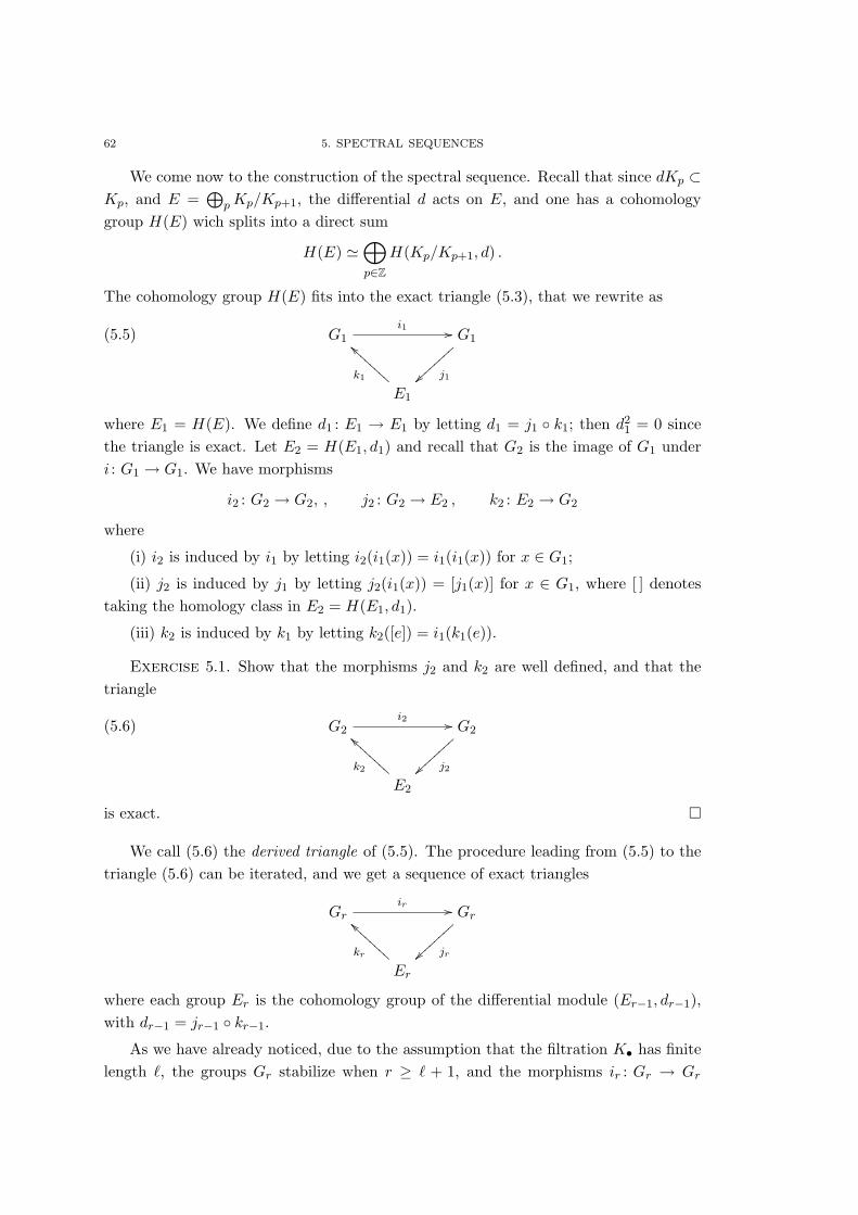
62 5. SPECTRAL SEQUENCES
We come now to the construction of the spectral sequence. Recall that since dKp ⊂Kp, and E =
⊕pKp/Kp+1, the differential d acts on E, and one has a cohomology
group H(E) wich splits into a direct sum
H(E) '⊕p∈Z
H(Kp/Kp+1, d) .
The cohomology group H(E) fits into the exact triangle (5.3), that we rewrite as
(5.5) G1i1 // G1
j1~~||||
||||
E1
k1
``BBBBBBBB
where E1 = H(E). We define d1 : E1 → E1 by letting d1 = j1 k1; then d21 = 0 since
the triangle is exact. Let E2 = H(E1, d1) and recall that G2 is the image of G1 underi : G1 → G1. We have morphisms
i2 : G2 → G2, , j2 : G2 → E2 , k2 : E2 → G2
where
(i) i2 is induced by i1 by letting i2(i1(x)) = i1(i1(x)) for x ∈ G1;
(ii) j2 is induced by j1 by letting j2(i1(x)) = [j1(x)] for x ∈ G1, where [ ] denotestaking the homology class in E2 = H(E1, d1).
(iii) k2 is induced by k1 by letting k2([e]) = i1(k1(e)).
Exercise 5.1. Show that the morphisms j2 and k2 are well defined, and that thetriangle
(5.6) G2i2 // G2
j2~~||||
||||
E2
k2
``BBBBBBBB
is exact.
We call (5.6) the derived triangle of (5.5). The procedure leading from (5.5) to thetriangle (5.6) can be iterated, and we get a sequence of exact triangles
Grir // Gr
jr~~||||
||||
Er
kr
``BBBBBBBB
where each group Er is the cohomology group of the differential module (Er−1, dr−1),with dr−1 = jr−1 kr−1.
As we have already noticed, due to the assumption that the filtration K• has finitelength `, the groups Gr stabilize when r ≥ ` + 1, and the morphisms ir : Gr → Gr
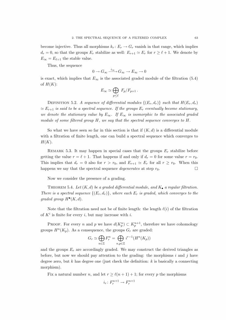
2. THE SPECTRAL SEQUENCE OF A FILTERED COMPLEX 63
become injective. Thus all morphisms kr : Er → Gr vanish in that range, which impliesdr = 0, so that the groups Er stabilize as well: Er+1 ' Er for r ≥ `+ 1. We denote byE∞ = E`+1 the stable value.
Thus, the sequence0→ G∞
i∞−−→G∞ → E∞ → 0
is exact, which implies that E∞ is the associated graded module of the filtration (5.4)of H(K):
E∞ '⊕p≤`
Fp/Fp+1 .
Definition 5.2. A sequence of differential modules (Er, dr) such that H(Er, dr)' Er+1 is said to be a spectral sequence. If the groups Er eventually become stationary,we denote the stationary value by E∞. If E∞ is isomorphic to the associated gradedmodule of some filtered group H, we say that the spectral sequence converges to H.
So what we have seen so far in this section is that if (K, d) is a differential modulewith a filtration of finite length, one can build a spectral sequence which converges toH(K).
Remark 5.3. It may happen in special cases that the groups Er stabilize beforegetting the value r = ` + 1. That happens if and only if dr = 0 for some value r = r0.This implies that dr = 0 also for r > r0, and Er+1 ' Er for all r ≥ r0. When thishappens we say that the spectral sequence degenerates at step r0.
Now we consider the presence of a grading.
Theorem 5.4. Let (K, d) be a graded differential module, and K• a regular filtration.There is a spectral sequence (Er, dr), where each Er is graded, which converges to thegraded group H•(K, d).
Note that the filtration need not be of finite length: the length `(i) of the filtrationof Ki is finite for every i, but may increase with i.
Proof. For every n and p we have d(Knp ) ⊂ Kn+1
p , therefore we have cohomologygroups Hn(Kp). As a consequence, the groups Gr are graded:
Gr '⊕n∈Z
Fnr =⊕n,p∈Z
ir−1(Hn(Kp))
and the groups Er are accordingly graded. We may construct the derived triangles asbefore, but now we should pay attention to the grading: the morphisms i and j havedegree zero, but k has degree one (just check the definition: k is basically a connectingmorphism).
Fix a natural number n, and let r ≥ `(n+ 1) + 1; for every p the morphisms
ir : Fn+1r → Fn+1
r
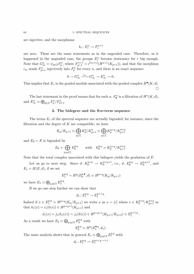
64 5. SPECTRAL SEQUENCES
are injective, and the morphisms
kr : Enr → Fn+1r
are zero. These are the same statements as in the ungraded case. Therefore, as ithappened in the ungraded case, the groups Enr become stationary for r big enough.Note that Gn∞ = ⊕p∈ZF
np , where Fn+1
p+1 = i`(n+1)(Hn+1(Kp+1)), and that the morphismi∞ sends Fnp+1 injectively into Fnp for every n, and there is an exact sequence
0→ Gn∞i∞−−→Gn∞ → En∞ → 0 .
This implies that Er is the graded module associated with the graded complex H•(K, d).
The last statement in the proof means that for each n, Fn• is a filtration of Hn(K, d),and En∞ '
⊕p∈Z F
np /F
np+1.
3. The bidegree and the five-term sequence
The terms Er of the spectral sequence are actually bigraded; for instance, since thefiltration and the degree of K are compatible, we have
Kp/Kp+1 '⊕q∈Z
Kqp/K
qp+1 '
⊕q∈Z
Kp+qp /Kp+q
p+1
and E0 = E is bigraded by
E0 =⊕p,q∈Z
Ep,q0 with Ep,q0 = Kp+qp /Kp+q
p+1 .
Note that the total complex associated with this bidegree yields the gradation of E.
Let us go to next step. Since d : Kp+qp → Kp+q+1
p , i.e., d : Ep,q0 → Ep,q+10 , and
E1 = H(E, d), if we set
Ep,q1 = Hq(Ep,•0 , d) ' Hp+q(Kp/Kp+1)
we have E1 '⊕
p,q∈ZEp,q1 .
If we go one step further we can show that
d1 : Ep,q1 → Ep+1,q1 .
Indeed if x ∈ Ep,q1 ' Hp+q(Kp/Kp+1) we write x as x = [e] where e ∈ Kp+qp /Kp+q
p+1 sothat k1(x) = i1(k(e)) ∈ Hp+q+1(Kp+1) and
d1(x) = j1(k1(x)) = j1(k(e)) ∈ Hp+q+1(Kp+1/Kp+2) ' Ep+1,q1 .
As a result we have E2 '⊕
p,q∈ZEp,q2 with
Ep,q2 ' Hp(E•,q1 , d1) .
The same analysis shows that in general Er '⊕
p,q∈ZEp,qr with
dr : Ep,qr → Ep+r,q−r+1r
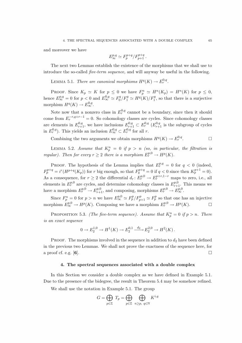
4. THE SPECTRAL SEQUENCES ASSOCIATED WITH A DOUBLE COMPLEX 65
and moreover we haveEp,q∞ ' F p+qp /F p+qp+1 .
The next two Lemmas establish the existence of the morphisms that we shall use tointroduce the so-called five-term sequence, and will anyway be useful in the following.
Lemma 5.1. There are canonical morphisms Hq(K)→ E0,qr .
Proof. Since Kp ' K for p ≤ 0 we have Fnp ' Hn(Kp) = Hn(K) for p ≤ 0,hence Ep,q∞ = 0 for p < 0 and E0,q
∞ ' F q0 /Fq1 ' Hq(K)/F q1 , so that there is a surjective
morphism Hq(K)→ E0,q∞ .
Note now that a nonzero class in E0,qr cannot be a boundary, since then it should
come from E−r,q+r−1r = 0. So cohomology classes are cycles. Since cohomology classes
are elements in E0,qr+1, we have inclusions E0,q
r+1 ⊂ E0,qr (E0,q
r+1 is the subgroup of cyclesin E0,q
r ). This yields an inclusion E0,q∞ ⊂ E0,q
r for all r.
Combining the two arguments we obtain morphisms Hq(K)→ E0,qr .
Lemma 5.2. Assume that Knp = 0 if p > n (so, in particular, the filtration is
regular). Then for every r ≥ 2 there is a morphism Ep,0r → Hp(K).
Proof. The hypothesis of the Lemma implies that Ep,qr = 0 for q < 0 (indeed,F p+qp = ir(Hp+q(Kp)) for r big enough, so that F p+qq = 0 if q < 0 since then Kp+1
p = 0).As a consequence, for r ≥ 2 the differential dr : Ep,0r → Ep+r,1−rr maps to zero, i.e., allelements in Ep,0r are cycles, and determine cohomology classes in Ep,0r+1. This means wehave a morphism Ep,0r → Ep,0r+1, and composing, morphisms Ep,0r → Ep,0∞ .
Since Fnp = 0 for p > n we have Ep,0∞ ' F pp /Fpp+1 ' F pp so that one has an injective
morphism Ep,0∞ → Hp(K). Composing we have a morphism Ep,0r → Hp(K).
Proposition 5.3. (The five-term sequence). Assume that Knp = 0 if p > n. There
is an exact sequence
0→ E1,02 → H1(K)→ E0,1
2d2−−→E2,0
2 → H2(K) .
Proof. The morphisms involved in the sequence in addition to d2 have been definedin the previous two Lemmas. We shall not prove the exactness of the sequence here, fora proof cf. e.g. [6].
4. The spectral sequences associated with a double complex
In this Section we consider a double complex as we have defined in Example 5.1.Due to the presence of the bidegree, the result in Theorem 5.4 may be somehow refined.
We shall use the notation in Example 5.1. The group
G =⊕p∈Z
Tp =⊕p∈Z
⊕n≥p, q∈N
Ki,q
66 5. SPECTRAL SEQUENCES
has natural gradation G = ⊕n∈ZGn given by
(5.7) Gn =⊕p∈Z
Tnp '⊕p∈Z
n−p⊕j=0
Kn−j,j
but it also bigraded, with bidegree
Gp,q = T p+qq .
Notice that if we form the total complex⊕
p+q=nGp,q we obtain the complex (5.7) back:
⊕p+q=n
Gp,q '⊕p+q=n
q⊕j=0
Kp+q−j,j =n−p⊕j=0
Kn−j,j = Gn .
The operators δ1, δ2 and d = δ1 + δ2 act on G:
δ1 : Gn,q → Gn+1,q , δ2 = Gn,q → Gn,q+1 , d : Gk → Gk+1 .
We analyze the spectral sequence associated with these data. The first three termsare easily described. One has
Ep,q0 ' T p+qp /T p+qp+1 ' Kp,q
so that the differential d0 : Ep,q0 → Ep,q+10 coincides with δ2 : Kp,q → Kp,q+1, and one
has
(5.8) Ep,q1 ' Hq(Kp,•, δ2) .
At next step we have d1 : Ep,q1 → Ep+1,q1 with Ep,q1 ' Hp+q(Tp/Tp+1) and Tp/Tp+1 '⊕
q∈Z Kp,q. Hence the differential
d1 : Hp+q(⊕n∈Z
Kp,n)→ Hp+q+1(⊕n∈Z
Kp+1,n)
is identified with δ1, and
(5.9) Ep,q2 ' Hp(E•,q1 , δ1) .
One should notice that by exchanging the two degrees in K (i.e., considering anotherdouble complex ′K such that ′Kp,q = Kq,p), we obtain another spectral sequence, thatwe denote by ′Er, ′dr. Both sequences converge to the same graded group, i.e., thecohomology of the total complex (but the corresponding filtrations are in general differ-ent), and this often provides interesting information. For the second spectral sequencewe get
′Eq,p1 ' Hp(K•,q, δ1)(5.10)′Eq,p2 ' Hq(′Ep,•1 , δ2) .(5.11)
4. THE SPECTRAL SEQUENCES ASSOCIATED WITH A DOUBLE COMPLEX 67
Example 5.1. A simple application of the two spectral sequences associated with adouble complex provides another proof of the Cech-de Rham theorem, i.e., the isomor-phism H•(X,R) ' H•DR(X) for a differentiable manifold X. Let U = Ui be a goodcover of X, and define the double complex
Kp,q = Cp(U,Ωq) ,
i.e., K•,q is the complex of Cech cochains of U with coefficients in the sheaf of differentialq-forms. The first differential δ1 is basically the Cech differential δ, while δ2 is theexterior differential d.3 Actually δ and d commute rather than anticommute, but thisis easily settled by defining the action of δ1 on Kp,q as δ1 = (−1)qδ (this of courseleaves the spaces of boundaries and cycles unchanged). We start analyzing the spectralsequences from the terms E1. For the first, we have
Ep,q1 ' Hq(Kp,•, d) '∏
i0<···<ip
HqDR(Ui0...ip) .
Since all Ui0...ip are contractible we have
Ep,01 ' Cp(U,R)
Ep,q1 = 0 for q 6= 0 .
As a consequence we have Ep,q2 = 0 for q 6= 0, while
Ep,02 ' Hp(C•(U,R), δ) = Hp(U,R) .
This implies that d2 = 0, so that the spectral sequence degenerates at the second step,and Ep,q∞ = 0 for q 6= 0 and Ep,0∞ ' Hp(U,R). The resulting filtration of Hp(T,D) hasonly one nonzero quotient, so that Hp(T,D) ' Hp(U,R).
Let us now consider the second spectral sequence. We have
′Ep,q1 ' Hq(K•,p, δ) = Hq(C•(U,Ωp), δ) = Hq(U,Ωp) .
Since the sheaves Ωp are acyclic, we have
Ep,01 ' H0(U,Ωp) ' Ωp(X)
Ep,q1 = 0 for q 6= 0 .
At next step we have therefore ′Ep,q2 = 0 for q 6= 0, and
′Ep,02 ' Hp(Ω•(X), d)) ' HpDR(X) .
Again the spectral sequence degenerates at the second step, and we have Hp(T,D) 'HpDR(X). Comparing with what we got from the first sequence, we obtain Hp
DR(X) 'Hp(U,R). Taking a direct limit on good covers, we obtain Hp(X,R) ' Hp
DR(X).
3Here a notational conflict arises, so that we shall denote by D the differential of the total complex
T .
68 5. SPECTRAL SEQUENCES
Remark 5.2. From this example we may get the general result that if at step r,with r ≥ 1, we have Ep,qr = 0 for q 6= 0 (or for p 6= 0) then the sequence degenerates atstep r, and Ep,0r ' Hp(T, d) (or E0,q
r ' Hq(T, d)).
5. Some applications
5.1. The spectral sequence of a resolution. In this section we extend Example5.1 to a much general situation. Let (L•, f) be a complex of sheaves on a paracompacttopological space X, and let U be an open cover of X. We introduce the double complexKp,q = Cp(U,Lq). We shall denote by Hq(L•) the cohomology sheaves of the complexL•. These are the sheaves associated with the quotient presheaves
Hq(U) =ker f : Lq(U)→ Lq+1(U)Im f : Lq−1(U)→ Lq(U)
.
The E1 term of the first spectral sequence is
Ep,q1 ' Hq(Kp,•, δ2) = Hq(Cp(U,L•), f)) ' Cp(U, Hq(L•)) .
The second term of the sequence is
Ep,q2 ' Hp(E•,q1 , δ1) ' Hp(C•(U, Hq(L•)), δ) ' Hp(U,Hq(L•))
where, since X is paracompact, we have replaced the presheaves H• with the corre-sponding sheaves H• (possibly replacing the cover U by a suitable refinement).
For the second spectral sequence we have
′Ep,q1 ' Hq(K•,p, δ1) ' Hq(C•(U,Lp), δ1) ' Hp(U,Lq)
′Eq,p2 ' Hp(′Eq,•1 , δ2) ' Hp(Hq(U,L•), f) .
Let assume now that L• is a resolution of a sheaf F ; then Hq(L•) = 0 for q 6= 0,and H0(L•) ' F . The first spectral sequence degenerates at the second step, and wehave Ep,q2 = 0 for q 6= 0 and Ep,02 ' Hp(U,F). The second spectral sequence does notdegenerate, but we may say that it converges to the graded group H•(U,F) (since thesame does the first sequence). By taking direct limit over the cover U, we have:
Proposition 5.1. Given a resolution L• of a sheaf F on a paracompact space X,there is a spectral sequence E• whose second term is E
p,q2 = Hq(Hp(X,L•), f), which
converges to the graded group H•(X,F).
The canonical filtrations of a double complex always satisfy the hypothesis of Lemma5.2. So, considering the first spectral sequence, we obtain morphisms (again taking adirect limit)
Hq(L•(X), f)→ Hq(X,F) .
5. SOME APPLICATIONS 69
In general these are not isomorphisms. The same morphisms could be obtained bybreaking the exact sequence 0 → F → L• into short exact sequences, taking the asso-ciated long exact cohomology sequences and suitably composing the morphisms, as inthe proof of the abstract de Rham theorem 3.14.
A further specialization is obtained if the resolution L• is acyclic; then the secondspectral sequence degenerates at the second step as well, and we get isomorphismsHp(X,F) ' Hp(L•(X), f), i.e., we have another proof of the abstract de Rham theorem3.14.
5.2. The spectral sequence of a fibred space. Let F be a sheaf on a para-compact space X and π : X → Y a continuous map, where Y is a second paracompactspace. We shall use the fact that every sheaf of abelian groups on space admits flabbyresolutions (cf. Sections 3.2.5 and 3.3). We shall associate a spectral sequence to thesedata. We consider the complex
(5.12) 0→ π∗F → π∗L0f−−→π∗L1
f−−→ . . .
where (L•, f) is a flabby resolution of F . The morphism π∗F → π∗L0 is injective, butotherwise the complex (5.12) is no longer exact. However, the sheaves π∗L• are flabby.We denote by Rkπ∗F the cohomology sheaves Hk(π∗L•).These sheaves are called thehigher direct images of F . Note that R0π∗F ' π∗F .
Proposition 5.2. The sheaf Rkπ∗F is isomorphic to the sheaf associated with thepresheaf Pk on Y defined by Pk(U) = Hk(π−1(U),F).
This implies that the sheaves Rkπ∗F do not depend, up to isomorphism, on thechoice of the resolution.
Proof. Rkπ∗F is by definition the sheaf associated with the presheaf
U ker f : Lk(π−1(U))→ Lk+1(π−1(U))Im f : Lk−1(π−1(U))→ Lk(π−1(U))
= Hk(L•(π−1(U), f) .
Since the restriction of a flabby sheaf to an open subset is flabby, by the abstract deRham theorem we have isomorphisms
Hk(L•(π−1(U), f) ' Hk(π−1(U),F) ,
whence the claim follows.
Let us consider the double complex Cp(U, π∗Lq), where U is a locally finite opencover of Y . The two spectral sequences we have previously studied yield at the secondterm
Ep,q2 ' Hp(U, Rqπ∗F)
′Ep,q2 ' Hq(Hp(U, π∗L•), f)

70 5. SPECTRAL SEQUENCES
Since the sheaves π∗L• are soft (hence acyclic) the second spectral sequence degenerates,and one has ′Ep,q∞ = 0 for p 6= 0, and
′E0,q∞ ' ′E0,q
2 ' Hq(H0(Y, π∗L•), f)
' Hq(L•(X), f) ' Hq(X,F) .
Again after taking a direct limit, we have:
Proposition 5.3. Given a continuous map of paracompact spaces π : X → Y and asheaf F on X, there is a spectral sequence E• whose second term is E
p,q2 = Hp(Y,Rqπ∗F),
which converges to the graded group H•(X,F).
We describe without proof the relation between the stalks of the sheaf Rkπ∗Fat points y ∈ Y and the cohomology groups Hk(π−1(y),F); here F is to be consid-ered as restricted to π−1, i.e., more precisely we should write Hk(π−1(y), i−1
y F) whereiy : π−1(y)→ X is the inclusion. Since
(Rkπ∗F )y = lim−→y∈U
(Rkπ∗F)(U) ' lim−→y∈U
Hk(π−1(U),F) ,
while Hk(π−1(y),F) is the direct limit of the groups Hk(V,F) where V ranges over allopen neighbourhoods of π−1(y), there is a natural map
(5.13) (Rkπ∗F)y → Hk(π−1(y),F) .
This is an isomorphism under some conditions, e.g., if Y is locally compact and π isproper (cf. [6]). This happens for instance when both X and Y are compact.
As a simple Corollary to Proposition 5.3 one obtains Leray’s theorem:
Corollary 5.4. If every point y ∈ Y has a system of neighbourhoods whose pre-images are acyclic for F , then Hk(X,F) ' Hk(Y, π∗F) for all k ≥ 0.
Proof. The hypothesis of the Corollary means that every y ∈ Y has a system ofneighbourhoods U such that Hk(π−1(U),F) = 0 for all k > 0. This implies thatRkπ∗F = 0 for k > 0, so that the only nonzero terms in the spectral sequence E2 areEp,02 ' Hp(Y, π∗F). The sequence degenerates and the claim follows.
5.3. The Kunneth theorem. Let X, Y be topological spaces, and G an abeliangroup. We shall denote by the same symbol G the corresponding constant sheaves onthe spaces X, Y and X × Y . The Kunneth theorem computes the cohomology groupsH•(X × Y,G) in terms of the groups H•(X,Z) and H•(Y,G).
We shall need the following version of the universal coefficient theorem.
Proposition 5.5. If X is a paracompact topological space and G a torsion-freegroup, then Hk(X,G) ' Hk(X,Z)⊗Z G for all k ≥ 0.
Proof. Cf. [21].
5. SOME APPLICATIONS 71
Proposition 5.6. Assume that the groups H•(Y,G) have no torsion over Z, andthat X and Y are compact Hausdorff and locally Euclidean. Then,
Hk(X × Y,G) '⊕p+q=k
Hp(X,Z)⊗Hq(Y,G) .
Proof. Let π : X × Y → X be the projection onto the first factor. If U is acontractible open set in U , then by the homotopic invariance of the cohomology withcoefficients in a constant sheaf (which follows e.g. from its isomorphism with singularcohomology) we have H•(U × Y,G) ' H•(Y,G). If V ⊂ U , the morphism H•(U ×Y,G) → H•(V × Y,G) corresponds to the identity of H•(Y,G). Under the presenthypotheses the morphism (5.13) is an isomorphism. These facts imply that Rpπ∗G is theconstant sheaf on X with stalk Hp(Y,G). The second term of the spectral sequence ofProposition 5.3 becomes E
p,q2 ' Hp(X,Hq(Y,G)). By the universal coefficient theorem,
since the groups Hq(Y,G) have no torsion over Z, we have Ep,q2 ' Hp(X,Z)⊗ZH
q(Y,G).

Part 2
Introduction to algebraic geometry

CHAPTER 6
Complex manifolds and vector bundles
In this chapter we give a sketchy introduction to complex manifolds. The reader isassumed to be acquainted with the rudiments of the theory of differentiable manifolds.
1. Basic definitions and examples
1.1. Holomorphic functions. Let U ⊂ C be an open subset. We say that afunction f : U → C is holomorphic if it is C1 and for all x ∈ U its differential Dfx : C→C is not only R-linear but also C-linear. If elements in C are written z = x + iy, andwe set f(x, y) = α(x, y) + iβ(x, y), then this condition can be written as
(6.1) αx = βy, αy = −βx
(these are the Cauchy-Riemann conditions). If we use z, z as variables, the Cauchy-Riemann conditions read fz = 0, i.e. the holomorphic functions are the C1 function ofthe variable z. Moreover, one can show that holomorphic functions are analytic.
The same definition can be given for holomorphic functions of several variables.
Definition 6.1. Two open subsets U , V of Cn are said to biholomorphic if thereexists a bijective holomorphic map f : U → V whose inverse is holomorphic. The mapf itself is then said to be biholomorphic.
1.2. Complex manifolds. Complex manifolds are defined as differentiable mani-folds, but requiring that the local model is Cn, and that the transition functions arebiholomorphic.
Definition 6.2. An n-dimensional complex manifold is a second countable Haus-dorff topological space X together with an open cover Ui and maps ψi : Ui → Cn whichare homeomorphisms onto their images, and are such that all transition functions
ψi ψ−1j : ψj(Ui ∩ Uj)→ ψi(Ui ∩ Uj)
are biholomorphisms.
Example 6.3. (The Riemann sphere) Consider the sphere in R3 centered at theorigin and having radius 1
2 , and identify the tangent planes at (0, 0, 12) and (0, 0,−1
2) withC. The stereographic projections give local complex coordinates z1, z2; the transitionfunction z2 = 1/z1 is defined in C? = C− 0 and is biholomorphic.
75
76 6. COMPLEX MANIFOLDS AND VECTOR BUNDLES
1-dimensional complex manifolds are called Riemann surfaces. Compact Riemannsurfaces play a distinguished role in algebraic geometry; they are all algebraic (i.e. theyare sets of zeroes of systems of homogeneous polynomials), as we shall see in Chapter8.
Example 6.4. (Projective spaces) We define the n-dimensional complex projectivespace as the space of complex lines through the origin of Cn+1, i.e.
Pn =Cn+1 − 0
C∗.
By standard topological arguments Pn with the quotient topology is a Hausdorff second-countable space.
Let π : Cn+1 − 0 → Pn be the projection, If w = (w0, . . . , wn) ∈ Cn+1 we shalldenote π(w) = [w0, . . . , wn]. The numbers (w0, . . . , wn) are said to be the homogeneouscoordinates of the point π(w). If (u0, . . . , un) is another set of homogeneous coordinatesfor π(w), then ui = λwi, with λ ∈ C∗ (i = 0, . . . , n).
Denote by Ui ⊂ Cn+1 the open set where wi 6= 0, let Ui = π(Ui), and define a map
ψi : Ui → Cn, ψ([w0, . . . , wn]) =(w0
wi, . . . ,
wi−1
wi,wi+1
wi, . . . ,
wn
wi
).
The sets Ui cover Pn, the maps ψi are homeomorphisms, and their transition functions
ψi ψ−1j : ψj(Uj)→ ψi(Ui),
ψi ψ−1j (z1, . . . , zn) =
(z1
zi, . . . ,
zi−1
zi,zi+1
zi, . . . ,
1zi, . . .
zn
zi
),
↑j-th argument
are biholomorphic, so that Pn is a complex manifold (we have assumed that i < j). Themap π restricted to the unit sphere in Cn+1 is surjective, so that Pn is compact. Theprevious formula for n = 1 shows that P1 is biholomorphic to the Riemann sphere.
The coordinates defined by the maps ψi, usually denoted (z1, . . . , zn), are calledaffine or Euclidean coordinates.
Example 6.5. (The general linear complex group). Let
Mk,n = k × n matrices with complex entries, k ≤ n
Mk,n = matrices in Mk,n of rank k, i.e.
Mk,n =⋃i=1
A ∈Mk,n such that detAi 6= 0
where Ai, . . . , A` are the k × k minors of A. Mk,n is a complex manifold of dimensionkn; Mk,n is an open subset in Mk,n, as its second description shows, so it is a complexmanifold of dimension kn as well. In particular, the general linear group Gl(n,C) =Mn,n is a complex manifold of dimension n2. Here are some of its relevant subgroups:
1. BASIC DEFINITIONS AND EXAMPLES 77
(i) U(n) = A ∈ Gl(n,C) such that AA† = I;(ii) SU(n) = A ∈ U(n) such that detA = 1;
these two groups are real (not complex!) manifolds, and dimR U(n) = n2, dimR SU(n) =n2 − 1.
(iii) the group Gl(k, n; C) formed by invertible complex matrices having a blockform
(6.2) M =
(A 0B C
)where the matrices A, B, C are k × k, (n− k)× k, and (n− k)× (n− k), respectively.Gl(k, n; C) is a complex manifold of dimension k2 +n2−nk. Since a matrix of the form(6.2) is invertible if and only if A and C are, while B can be any matrix, Gl(k, n; C) isbiholomorphic to the product manifold Gl(k,C)×Gl(n− k,C)×Mk,n.
1.3. Submanifolds. Given a complex manifold X, a submanifold of X is a pair(Y, ι), where Y is a complex manifold, and ι : Y → X is an injective holomorphic mapwhose jacobian matrix has rank equal to the dimension of Y at any point of Y (of courseY can be thought of as a subset of X).
Example 6.6. Gl(k, n; C) is a submanifold of Gl(n,C).
Example 6.7. For any k < n the inclusion of Ck+1 into Cn+1 obtained by settingto zero the last n− k coordinates in Cn+1 yields a map Pk → Pn; the reader may checkthat this realizes Pk as a submanifold of Pn.
Example 6.8. (Grassmann varieties) Let
Gk,n = space of k-dimensional planes in Cn
(so G1,n ≡ Pn − 1). This is the Grassmann variety of k-planes in Cn. Given a k-plane,the action of Gl(n,C) on it yields another plane (possibly coinciding with the previousone). The subgroup of Gl(n,C) which leaves the given k-plane fixed is isomorphic toGl(k, n; C), so that
Gk,n 'Gl(n,C)Gl(k, n; C)
.
As the reader may check, this representation gives Gk,n the structure of a complexmanifold of dimension k(n−k). Since in the previous reasoning Gl(n,C) can be replacedby U(n), and since Gl(k, n; C)∩U(n) = U(k)×U(n−k), we also have the representation
Gk,n 'U(n)
U(k)× U(n− k)
showing that Gk,n is compact.
An element in Gk,n singles out (up to a complex factor) a decomposable element inΛkCn,
λ = v1 ∧ · · · ∧ vk
78 6. COMPLEX MANIFOLDS AND VECTOR BUNDLES
where the vi are a basis of tangent vectors to the given k-plane. So Gk,n imbeds intoP(ΛkCn) = PN , where N =
((nk
))− 1 (this is called the Plucker embedding. If a basis
v1, . . . , vn is fixed in Cn, one has a representation
λ =n∑
i1,...,ik=1
Pi1...ik vi1 ∧ · · · ∧ vik ;
the numbers Pi1...ik are the Plucker coordinates on the Grassmann variety.
2. Some properties of complex manifolds
2.1. Orientation. All complex manifolds are oriented. Consider for simplicity the1-dimensional case; the jacobian matrix of a transition function z′ = f(z) = α(x, y) +iβ(x, y) is (by the Cauchy-Riemann conditions)
J =
(αx αy
βx βy
)=
(αx αy
−αy αx
)so that detJ = α2
x + α2y > 0, and the manifold is oriented.
Notice that we may always conjugate the complex structure, considering (e.g. in the
1-dimensional case) the coordinate change z 7→ z; in this case we have J =
(1 00 −1
),
so that the orientation gets reversed.
2.2. Forms of type (p, q). Let X be an n-dimensional complex manifold; by theidentification Cn ' R2n, and since a biholomorphic map is a C∞ diffeomorphism, Xhas an underlying structure of 2n-dimensional real manifold. Let TX be the smoothtangent bundle (i.e. the collection of all ordinary tangent spaces to X). If (z1, . . . , zn) isa set of local complex coordinates around a point x ∈ X, then the complexified tangentspace TxX ⊗R C admits the basis((
∂
∂z1
)x
, . . . ,
(∂
∂zn
)x
,
(∂
∂z1
)x
, . . . ,
(∂
∂zn
)x
).
This yields a decomposition
TX ⊗ C = T ′X ⊕ T ′′X
which is intrinsic because X has a complex structure, so that the transition functionsare holomorphic and do not mix the vectors ∂
∂ziwith the ∂
∂zi. As a consequence one has
a decomposition
ΛiT ∗X ⊗ C =⊕p+q=i
Ωp,qX where Ωp,qX = Λp(T ′X)∗ ⊗ Λq(T ′′X)∗ .
The elements in Ωp,qX are called differential forms of type (p, q), and can locally bewritten as
η = ηi1...ip,j1...jq(z, z) dzi1 ∧ · · · ∧ dzip ∧ dzj1 ∧ · · · ∧ dzjq .
4. HOLOMORPHIC VECTOR BUNDLES 79
The compositions
Ωp+1,qX
Ωp,qXd // Λp+q+1T ∗X
∂77ooooooooooo
∂ ''OOOOOOOOOOO
Ωp,q+1X
define differential operators ∂, ∂ such that
∂2 = ∂2 = ∂∂ + ∂∂ = 0
(notice that the Cauchy-Riemann condition can be written as ∂f = 0).
3. Dolbeault cohomology
Another interesting cohomology theory one can consider is the Dolbeault cohomologyassociated with a complex manifold X. Let Ωp,q denote the sheaf of forms of type (p, q)on X. The Dolbeault (or Cauchy-Riemann) operator ∂ : Ωp,q → Ωp,q+1 squares to zero.Therefore, the pair (Ωp,•(X), ∂) is for any p ≥ 0 a cohomology complex. Its cohomologygroups are denoted by Hp,q
∂(X), and are called the Dolbeault cohomology groups of X.
We have for this theory an analogue of the Poincare Lemma, which is sometimescalled the ∂-Poincare Lemma (or Dolbeault or Grothendieck Lemma).
Proposition 6.1. Let ∆ be a polycylinder in Cn (that is, the cartesian product ofdisks in C). Then Hp,q
∂(∆) = 0 for q ≥ 1.
Proof. Cf. [10].
Moreover, the kernel of the morphism ∂ : Ωp,0 → Ωp,1 is the sheaf of holomorphicp-forms Ωp. Therefore, the Dolbeault complex of sheaves Ωp,• is a resolution of Ωp,i.e. for all p = 0, . . . , n (where n = dimCX) the sheaf sequence
0→ Ωp → Ωp,0 ∂−−→Ωp,1 ∂−−→ . . .∂−−→Ωp,1 → 0
is exact. Moreover, the sheaves Ωp,q are fine (they are C∞X -modules). Then, exactly asone proves the de Rham theorem (Theorem 3.3.15), one obtains the Dolbeault theorem:
Proposition 6.2. Let X be a complex manifold. For all p, q ≥ 0, the cohomologygroups Hp,q
∂(X) and Hq(X,Ωp) are isomorphic.
4. Holomorphic vector bundles
4.1. Basic definitions. Holomorphic vector bundles on a complex manifold X aredefined in the same way than smooth complex vector bundles, but requiring that all themaps involved are holomorphic.
80 6. COMPLEX MANIFOLDS AND VECTOR BUNDLES
Definition 6.1. A complex manifold E is a rank n holomorphic vector bundle onX if there are
(i) an open cover Uα of X
(ii) a holomorphic map π : E → X
(iii) holomorphic maps ψα : π−1(Uα)→ Uα × Cn
such that
(i) π = pr1 ψα, where = pr1 is the projection onto the first factor of Uα × Cn;
(ii) for all p ∈ Uα ∩ Uβ, the map
pr2 ψβ ψ−1α (p, •) : Cn → Cn
is a linear isomorphism.
Vector bundles of rank 1 are called line bundles.
With the data that define a holomorphic vector bundle we may construct holomor-phic maps
gαβ : Uα ∩ Uβ → Gl(n,C)
given bygαβ(p) · x = pr2 ψα ψ−1
β (ψ, x) .
These maps satisfy the cocycle condition
gαβ gβγ gγα = Id on Uα ∩ Uβ ∩ Uγ .
The collection Uα, ψα is a trivialization of E.
For every x ∈ X, the subset Ex = π−1(x) ⊂ E is called the fibre of E over x. Bymeans of a trivialization around x, Ex is given the structure of a vector space, which isactually independent of the trivialization.
A morphism between two vector bundles E, F over X is a holomorphic map f : E →F such that for every x ∈ X one has f(Ex) ⊂ Fx, and such that the resulting mapfx : Ex → Fx is linear. If f is a biholomorphism, it is said to be an isomorphism ofvector bundles, and E and F are said to be isomorphic.
A holomorphic section of E over an open subset U ⊂ X is a holomorphic maps : U → E such that π s = Id. With reference to the notation previously introduced,the maps
s(α)i : Uα → E, s(α)i(x) = ψ−1α (x, ei), i = 1, . . . , n
where ei is the canonical basis of Cn, are sections of E over Uα. Let E(Uα) denotethe set of sections of E over Uα; it is a free module over the ring O(Uα) of holomorphicfunctions on Uα, and its subset s(α)ii=1,...,n is a basis. On an intersection Uα ∩Uβ onehas the relation
s(α)i =n∑k=1
(gαβ)ik s(β)k.
4. HOLOMORPHIC VECTOR BUNDLES 81
Exercise 6.2. Show that two trivializations are equivalent (i.e. describe isomorphicbundles) if there exist holomorphic maps λα : Uα → Gl(n,C) such that
(6.3) g′αβ = λα gαβ λ−1β
Exercise 6.3. Show that the rule that to any open subset U ⊂ X assigns theO∞X (U)-module of sections of a holomorphic vector bundle E defines a sheaf E (whichactually is a sheaf of OX -modules).
If E is a holomorphic (or smooth complex) vector bundle, with transition functionsgαβ, then the maps
(6.4) g′αβ = (gTαβ)−1
(where T denotes transposition) define another vector bundle, called the dual vectorbundle to E, and denoted by E∗. Sections of E∗ can be paired with (or act on) sectionsof E, yielding holomorphic (smooth complex-valued) functions on (open sets of) X.
Example 6.4. The space E = X × Cn, with the projection onto the first factor, isobviously a holomorphic vector bundle, called the trivial vector bundle of rank n. Weshall denote such a bundle by Cn (in particular, C denotes the trivial line bundle). Aholomorphic vector bundle is said to be trivial when it is isomorphic to Cn.
Every holomorphic vector bundle has an obvious structure of smooth complex vectorbundle. A holomorphic vector bundle may be trivial as a smooth bundle while not beingtrivial as a holomorphic bundle. (In the next sections we shall learn some homologicaltechniques that can be used to handle such situations).
Example 6.5. (The tangent and cotangent bundles) If X is a complex manifold,the “holomorphic part” T ′X of the complexified tangent bundle is a holomorphic vectorbundle, whose rank equals the complex dimension of X. Given a holomorphic atlasfor X, the locally defined holomorphic vector fields ∂
∂z1. . . , ∂
∂zn provide a holomorphictrivialization of X, such that the transition functions of T ′X are the jacobian matricesof the transition functions of X. The dual of T ′X is the holomorphic cotangent bundleof X.
Example 6.6. (The tautological bundle) Let (w1, . . . , wn+1) be homogeneous coor-dinates in Pn. If to any p ∈ Pn (which is a line in Cn+1) we associate that line we obtaina line bundle, the tautological line bundle L of Pn. To be more concrete, let us exhibita trivialization for L and the related transition functions. If Ui is the standard coverof Pn, and p ∈ Ui, then wi can be used to parametrize the points in the line p. So ifp has homogeneous coordinates (w0, . . . , wn), we may define ψi : π−1(Ui) → Ui × C asψi(u) = (p, wi) if p = π(u). The transition function is then gik = wi/wk. The dualbundle H = L∗ acts on L, so that its fibre at p = π(u), u ∈ Cn+1 can be regarded as
82 6. COMPLEX MANIFOLDS AND VECTOR BUNDLES
the space of linear functionals on the line Cu ≡ Lp, i.e. as hyperplanes in Cn+1. HenceH is called the hyperplane bundle. Often L is denoted O(−1), and H is denoted O(1)— the reason of this notation will be clear in Chapter 7.
In the same way one defines a tautological bundle on the Grassmann variety Gk,n;it has rank k.
Exercise 6.7. Show that that the elements of a basis of the vector space of globalsections of L can be identified homogeneous coordinates, so that dimH0(Pn, L) = n +1. Show that the global sections of H can be identified with the linear polynomialsin the homogeneous coordinates. Hence, the global sections of Hr are homogeneouspolynomials of order r in the homogeneous coordinates.
4.2. More constructions. Additional operations that one can perform on vectorbundles are again easily described in terms of transition functions.
(1) Given two vector bundles E1 and E2, of rank r1 and r2, their direct sum E1⊕E2
is the vector bundle of rank r1 + r2 whose transition functions have the block matrixform (
g(1)αβ 0
0 g(2)αβ
)(2) We may also define the tensor product E1 ⊗ E2, which has rank r1r2 and has
transition functions g(1)αβ g
(2)αβ . This means the following: assume that E1 and E2 trivialize
over the same cover Uα, a condition we may always meet, and that in the giventrivializations, E1 and E2 have local bases of sections s(α)i and t(α)k. Then E1⊗E2
has local bases of sections s(α)i⊗ t(α)k and the corresponding transition functions aregiven by
s(α)i ⊗ t(α)k =r1∑m=1
r2∑n=1
(g(1)αβ )im(g(2)
αβ )kn s(β)m ⊗ t(β)n .
In particular the tensor product of line bundles is a line bundle. If L is a linebundle, one writes Ln for L ⊗ · · · ⊗ L (n factors). If L is the tautological line bundleon a projective space, one often writes Ln = O(−n), and similarly Hn = O(n) (noticethat O(−n)∗ = O(n)).
(3) If E is a vector bundle with transition functions gαβ, we define its determinantdetE as the line bundle whose transition functions are the functions det gαβ. Thedeterminant bundle of the holomorphic tangent bundle to a complex manifold is calledthe canonical bundle K.
Exercise 6.8. Show that the canonical bundle of the projective space Pn is isomor-phic to O(−n− 1).
Example 6.9. Let π : Cn+1 − 0 → Pn be the usual projection, and let (w1, . . . ,
wn+1) be homogeneous coordinates in Pn. The tangent spaces to Pn are generated by
5. CHERN CLASSES 83
the vectors π∗ ∂∂wi
, and these are subject to the relation
n+1∑i=1
wi π∗∂
∂wi= 0 .
If ` is a linear functional on Cn+1 the vector field
v(w) = `(w)∂
∂wi
(i is fixed) satisfies v(λw) = λ v(w) and therefore descends to Pn. One can then definea map
E : H⊕(n+1) → TPn
(σ1, . . . , σn+1) 7→n+1∑i=1
σi(w)∂
∂wi
(recall that the sections of H can be regarded as linear functionals on the homogeneouscoordinates). The map E is apparently surjective. Its kernel is generated by the sectionσi(w) = wi, i = 1, . . . , n+ 1; notice that this is the image of the map
C→ H⊕(n+1), 1 7→ (w1, . . . , wn+1) .
The morphism H⊕(n+1) → TPn may be regarded as a sheaf morphism OPn(1)⊕(n+1)
→ TPn, the second sheaf being the tangent sheaf of Pn, i.e., the sheaf of germs ofholomorphic vector fields on Pn, and one has an exact sequence
0→ OPn → OPn(1)⊕(n+1) → TPn → 0
called the Euler sequence.
5. Chern class of line bundles
5.1. Chern classes of holomorphic line bundles. Let X a complex manifold.We define Pic(X) (the Picard group of X) as the set of holomorphic line bundles on Xmodulo isomorphism. The group structure of Pic(X) is induced by the tensor productof line bundles L⊗L′; in particular one has L⊗L∗ ' C (think of it in terms of transitionfunctions — here C denotes the trivial line bundle, whose class [C] is the identity inPic(X)), so that the class [L∗] is the inverse in Pic(X) of the class [L].
Let O denote the sheaf of holomorphic functions on X, and O∗ the subsheaf ofnowhere vanishing holomorphic funtions. If L ' L′ then the transition functions gαβ,g′αβ of the two bundles with respect to a cover Uα of X are 2-cocycles O∗, and satisfy
g′αβ = gαβλαλβ
with λα ∈ O∗(Uα),
so that one has an identification Pic(X) ' H1(X,O∗). The long cohomology sequenceassociated with the exact sequence
0→ Z→ O exp−−→O∗ → 0
84 6. COMPLEX MANIFOLDS AND VECTOR BUNDLES
(where exp f = e2πif ) contains the segment
H1(X,Z)→ H1(X,O)→ H1(X,O∗) δ−−→H2(X,Z)→ H2(X,O)
where δ is the connecting morphism. Given a line bundle L, the element
c1(L) = δ([L]) ∈ H2(X,Z)
is the first Chern class1 of L. The fact that δ is a group morphism means that
c1(L⊗ L′) = c1(L) + c1(L′) .
In general, the morphism δ is neither injective nor surjective, so that
(i) the first Chern class does not classify the holomorphic line bundles on X; thegroup
Pic0(X) = ker δ ' H1(X,O)/ ImH1(X,Z)
classifies the line bundles having the same first Chern class.
(ii) not every element in H2(X,Z) is the first Chern class of a holomorphic linebundle.
The image of c1 is a subgroup NS(X) of H2(X,Z), called the Neron-Severi group of X.
Exercise 6.1. Show that all line bundles on Cn are trivial.
Exercise 6.2. Show that there exist nontrivial holomorphic line bundles which aretrivial as smooth complex line bundles.
Notice that when X is compact the sequence
0→ H0(X,Z)→ H0(X,O)→ H0(X,O∗)→ 0
is exact, so that Pic0(X) = H1(X,O)/H1(X,Z). If in addition dimX = 1 we haveH2(X,O) = 0, so that every element inH2(X,Z) is the first Chern class of a holomorphicline bundle.2
From the definition of connecting morphism we can deduce an explicit formula fora Cech cocycle representing c1(L) with respect to the cover Uα:
c1(L)αβγ = 12πi (log gαβ + log gβγ + log gγα) .
From this one can easily prove that, if f : X → Y is a holomorphic map, and L is a linebundle on Y , then
c1(f∗L) = f ](c1(L)) .
1This allows us also to define the first Chern class of a vector bundle E of any rank by letting
c1(E) = c1(detE).2Here we use the fact that if X is a complex manifold of dimension n, then Hk(X,O) = 0 for all
k > n.
6. CHERN CLASSES 85
5.2. Smooth line bundles. The first Chern class can equally well be definedfor smooth complex line bundles. In this case we consider the sheaf C of complex-valued smooth functions on a differentiable manifold X, and the subsheaf C∗ of nowherevanishing functions of such type. The set of isomorphism classes of smooth complex linebundles is identified with the cohomology group H1(X, C∗). However now the sheaf Cis acyclic, so that the obstruction morphism δ establishes an isomorphism H1(X, C∗) 'H2(X,Z). The first Chern class of a line bundle L is again defined as c1(L) = δ([L]),but now c1(L) classifies the bundle (i.e. L ' L′ if and only if c1(L) = c1(L′)).
Exercise 6.3. (A rather pedantic one, to be honest...) Show that if X is a complexmanifold, and L is a holomorphic line bundle on it, the first Chern classes of L regardedas a holomorphic or smooth complex line bundle coincide. (Hint: start from the inclusionO → C, write from it a diagram of exact sequences, and take it to cohomology ...)
6. Chern classes of vector bundles
In this section we define higher Chern classes for complex vector bundles of any rank.Since the Chern classes of a vector bundle will depend only on its smooth structure, wemay consider a smooth complex vector bundle E on a differentiable manifold X. Weare already able to define the first Chern class c1(L) of a line bundle L, and we knowthat c1(L) ∈ H2(X,Z). We proceed in two steps:
(1) we first define Chern classes of vector bundles that are direct sums of line bundles;
(2) and then show that by means of an operation called cohomology base change wecan always reduce the computation of Chern classes to the previous situation.
Step 1. Let σi, i = 1 . . . k, denote the symmetric function of order i in k arguments.3.Since these functions are polynomials with integer coefficients, they can be regarded asfunctions on the cohomology ring H•(X,Z). In particular, if α1, . . . , αk are classes inH2(X,Z), we have σi(α1, . . . , αk) ∈ H2i(X,Z).
If E = L1⊕ · · · ⊕Lk, where the Li’s are line bundles, for i = 1...k we define the i-thChern class of E as
ci(E) = σi(c1(L1), . . . , c1(Lk)) ∈ H2i(X,Z) .
3The symmetric functions are defined as
σi(x1, . . . , xk) =X
1≤j1<···<ji≤n
xj1 · · · · · xji .
Thus, for instance,
σ1(x1, . . . , xk) = x1 + · · ·+ xk
σ2(x1, . . . , xk) = x1x2 + x1x3 + · · ·+ xk−1xk
. . .
σk(x1, . . . , xk) = x1 · · · · · xk.
As a first reference for symmetric functions see e.g. [24].
86 6. COMPLEX MANIFOLDS AND VECTOR BUNDLES
We also set c0(E) = 1; identifying H0(X,Z) with Z (assuming that X is connected) wemay think that c0(E) ∈ H0(X,Z).
Step 2 relies on the following result (sometimes called the splitting principle), whichwe do not prove here.
Proposition 6.1. Let E be a complex vector bundle on a differentiable manifoldX. There exists a differentiable map f : Y → X, where Y is a differentiable manifold,such that
(1) the pullback bundle f∗E is a direct sum of line bundles;
(2) the morphism f ] : H•(X,Z)→ H•(Y,Z) is injective;
(3) the Chern classes ci(f∗E) lie in the image of the morphism f ].
Definition 6.2. The i-th Chern class ci(E) of E is the unique class in H2i(X,Z)such that f ](ci(E)) = ci(f∗E).
We also define the total Chern class of E as
c(E) =k∑i=0
ci(E) ∈ H•(X,Z) .
The main property of the Chern classes are the following.
(1) If two vector bundles on X are isomorphic, their Chern classes coincide.
(2) Functoriality: if f : Y → X is a differentiable map of differentiable manifolds,and E is a complex vector bundle on X, then
f ](ci(E)) = ci(f∗E) .
(3) Whitney product formula: if E, F are complex vector bundles on X, then
c(E ⊕ F ) = c(E) ∪ c(F ) .
(4) Normalization: identify the cohomology group H2(Pn,Z) with Z by identifyingthe class of the hyperplane H with 1 ∈ Z. Then c1(H) = 1.
These properties characterize uniquely the Chern classes (cf. e.g. [14]). Notice that,in view of the splitting principle, it is enough to prove the properties (1), (2), (3) whenE and F are line bundles. Then (1) and (2) are already known, and (3) follows fromelementary properties of the symmetric functions.
The reader can easily check that all Chern classes (but for c0, obviously) of a trivialvector bundle vanish. Thus, Chern classes in some sense measure the twisting of abundle. It should be noted that, even in smooth case, Chern classes do not in generalclassify vector bundles, even as smooth bundles (i.e., generally speaking, c(E) = c(F )does not imply E ' F ). However, in some specific instances this may happen.
Exercise 6.3. Prove that for any vector bundle E one has c1(E) = c1(detE).
7. KODAIRA-SERRE DUALITY 87
7. Kodaira-Serre duality
In this section we introduce Kodaira-Serre duality, which will be one of the maintools in our study of algebraic curves. To start with a simple situation, let us studythe analogous result in de Rham theory. Let X be a differentiable manifold. Since theexterior product of two closed forms is a closed form, one can define a bilinear map
H iDR(X)⊗Hj
DR(X)→ H i+jDR(X), [τ ]⊗ [ω]→ [τ ∧ ω].
As we already know, via the Cech-de Rham isomorphism this product can be identifiedwith the cup product. If X is compact and oriented, by composition with the map4
∫X
: HnDR(X)→ R, ∫
X[ω] =
∫Xω
where n = dimX, we obtain a pairing
H iDR(X)⊗Hn−i
DR (X)→ R, [τ ]⊗ [ω]→ ∫X
[τ ∧ ω]
which is quite easily seen to be nondegenerate. Thus one has an isomorphism
H iDR(X)∗ ' Hn−i
DR (X)
(this is a form of Poincare duality).
If X is an n-dimensional compact complex manifold, in the same way we obtain anondegenerate pairing between Dolbeault cohomology groups
(6.5) Hp,q
∂(X)⊗Hn−p,n−q
∂(X)→ C,
and a duality
Hp,q
∂(X)∗ ' Hn−p,n−q
∂(X).
Exercise 6.1. (1) Let E be a holomorphic vector bundle on a complex manifoldX, denote by E the sheaf of its holomorphic sections, and by E∞ the sheaf of its smoothsections. Show (using a local trivialization and proving that the result is independentof the trivialization) that one can define a C-linear sheaf morphism
(6.6) ∂E : E∞ → Ω0,1 ⊗ E∞
which obeys a Leibniz rule
∂E(fs) = f∂Es+ ∂f ⊗ s
for s ∈ E∞(U), f ∈ C∞(U).
(2) Show that ∂E defines an exact sequence of sheaves
(6.7) 0→ Ωp ⊗ E → Ωp,0 ⊗ E∞ ∂E−−→Ωp,1 ⊗ E∞ ∂E−−→ . . .∂E−−→Ωp,n ⊗ E∞ → 0.
4This map is well defined because different representatives of [ω] differ by an exact form, whose
integral over X vanishes.
88 6. COMPLEX MANIFOLDS AND VECTOR BUNDLES
Here Ωp is the sheaf of holomorphic p-forms. In particular, E = ker(∂E : E∞ → Ω0,1 ⊗E∞).
(3) By taking global sections in (6.7), and taking coholomology from the resulting (ingeneral) non-exact sequence, one defines Dolbeault cohomology groups with coefficientsin E, denoted Hp,q
∂(X,E). Use the same argument as in the proof of de Rham’s theorem
to prove an isomorphism
(6.8) Hp,q
∂(X,E) ' Hq(X,Ωp ⊗ E).
By combining the pairing (6.5) with the action of the sections of E∗ on the sectionsof E we obtain a nondegenerate pairing
Hp,q
∂(X,E)⊗Hn−p,n−q
∂(X,E∗)→ C
and therefore a duality
Hp,q
∂(X,E)∗ ' Hn−p,n−q
∂(X,E∗).
Using the isomorphism (6.8) we can express this duality in the form
Hp(X,Ωq ⊗ E)∗ ' Hn−p(X,Ωn−q ⊗ E∗).
This is the Kodaira-Serre duality. In particular for q = 0 we get (denoting K = Ωn =detT ∗X, the canonical bundle of X)
Hp(X, E)∗ ' Hn−p(X,K ⊗ E∗).
This is usually called Serre duality.
8. Connections
In this section we give the basic definitions and sketch the main properties of con-nections. The concept of connection provides the correct notion of differential operatorto differentiate the sections of a vector bundle.
8.1. Basic definitions. Let E a complex, in general smooth, vector bundle on adifferentiable manifold X. We shall denote by E the sheaf of sections of E, and by Ω1
X
the sheaf of differential 1-forms on X. A connection is a sheaf morphism
∇ : E → Ω1X ⊗ E
satisfying a Leibniz rule∇(fs) = f∇(s) + df ⊗ s
for every section s of E and every function f on X (or on an open subset). The Leibnizrule also shows that ∇ is C-linear. The connection ∇ can be made to act on all sheavesΩkX ⊗ E , thus getting a morphism
∇ : ΩkX ⊗ E → Ωk+1
X ⊗ E ,
8. CONNECTIONS 89
by letting∇(ω ⊗ s) = dω ⊗ s+ (−1)kω ⊗∇(s).
If Uα is a cover of X over which E trivializes, we may choose on any Uα a setsα of basis sections of E(Uα) (notice that this is a set of r sections, with r = rkE).Over these bases the connection ∇ is locally represented by matrix-valued differential1-forms ωα:
∇(sα) = ωα ⊗ sα .
Every ωα is as an r × r matrix of 1-forms. The ωα’s are called connection 1-forms.
Exercise 6.1. Prove that if gαβ denotes the transition functions of E with respectto the chosen local basis sections (i.e., sα = gαβ sβ), the transformation formula for theconnection 1-forms is
(6.9) ωα = gαβ ωβ g−1αβ + dgαβ g
−1αβ .
The connection is not a tensorial morphism, but rather satifies a Leibniz rule; as aconsequence, the transformation properties of the connection 1-forms are inhomogeneousand contain an affine term.
Exercise 6.2. Prove that if E and F are vector bundles, with connections ∇1 and∇2, then the rule
∇(s⊗ t) = ∇1(s)⊗ t+ s⊗∇2(t)
(minimal coupling) defines a connection on the bundle E⊗F (here s and t are sectionsof E and F , respectively).
Exercise 6.3. Prove that is E is a vector bundle with a connection ∇, the rule
< ∇∗(τ), s >= d < τ, s > − < τ,∇(s) >
defines a connection on the dual bundle E∗ (here τ , s are sections of E∗ and E, respec-tively, and < , > denotes the pairing between sections of E∗ and E).
It is an easy exercise, which we leave to the reader, to check that the square of theconnection
∇2 : ΩkX ⊗ E → Ωk+2
X ⊗ E
is f -linear, i.e., it satisfies the property
∇2(fs) = f∇2(s)
for every function f on X. In other terms, ∇2 is an endomorphism of the bundle Ewith coefficients in 2-forms, namely, a global section of the bundle Ω2
X ⊗ End(E). It iscalled the curvature of the connection ∇, and we shall denote it by Θ. On local basissections sα it is represented by the curvature 2-forms Θα defined by
Θ(sα) = Θα ⊗ sα.
90 6. COMPLEX MANIFOLDS AND VECTOR BUNDLES
Exercise 6.4. Prove that the curvature 2-forms may be expressed in terms of theconnection 1-forms by the equation (Cartan’s structure equation)
(6.10) Θα = dωα − ωα ∧ ωα .
Exercise 6.5. Prove that the transformation formula for the curvature 2-forms is
Θα = gαβ Θβ g−1αβ .
Due to the tensorial nature of the curvature morphism, the curvature 2-forms obey ahomogeneous transformation rule, without affine term.
Since we are able to induce connections on tensor products of vector bundles (andalso on direct sums, in the obvious way), and on the dual of a bundle, we can induceconnections on a variety of bundles associated to given vector bundles with connec-tions, and thus differentiate their sections. The result of such a differentiation is calledthe covariant differential of the section. In particular, given a vector bundle E withconnection ∇, we may differentiate its curvature as a section of Ω2
X ⊗ End(E).
Proposition 6.6. (Bianchi identity) The covariant differential of the curvature ofa connection is zero, ∇Θ = 0.
Proof. A simple computation shows that locally ∇Θ is represented by the matrix-valued 3-forms
dΘα + ωα ∧Θα −Θα ∧ ωα .
By plugging in the structure equation (6.10) we obtain ∇Θ = 0.
8.2. Connections and holomorphic structures. If X is a complex manifold,and E a C∞ complex vector bundle on it with a connection ∇, we may split the latterinto its (1,0) and (0,1) parts, ∇′ and ∇′′, according to the splitting Ω1
X⊗C = Ω1,0X ⊕Ω0,1
X .
Analogously, the curvature splits into its (2,0), (1,1) and (0,2) parts,
Θ = Θ2,0 + Θ1,1 + Θ0,2 .
Obviously we have
Θ2,0 = (∇′)2, Θ1,1 = ∇′ ∇′′ +∇′′ ∇′, Θ0,2 = (∇′′)2.
In particular ∇′′ is a morphism Ωp,qX ⊗ E → Ωp,q+1
X ⊗ E . If Θ0,2 = 0, then ∇′′ is adifferential for the complex Ωp,•
X ⊗E . The same condition implies that the kernel of themap
(6.11) ∇′′ : E → Ω0,1X ⊗ E
has enough sections to be the sheaf of sections of a holomorphic vector bundle.
8. CONNECTIONS 91
Proposition 6.7. If Θ0,2 = 0, then the C∞ vector bundle E admits a uniqueholomorphic structure, such that the corresponding sheaf of holomorphic sections is iso-morphic to the kernel of the operator (6.11). Moreover, under this isomorphism theoperator (6.11) concides with the operator δE defined in Exercise 6.1.
Proof. Cf. [18], p. 9.
Conversely, if E is a holomophic vector bundle, a connection ∇ on E is said to becompatible with the holomorphic structure of E if ∇′′ = ∂E .
8.3. Hermitian bundles. A Hermitian metric h of a complex vector bundle E isa global section of E ⊗ E∗ which when restricted to the fibres yields a Hermitian formon them (more informally, it is a smoothly varying assignation of Hermitian structureson the fibres of E). On a local basis of sections sα, of E, h is represented by matriceshα of functions on Uα which, when evaluated at any point of Uα, are Hermitian andpositive definite. The local basis is said to be unitary if the corresponding matrix h isthe identity matrix.
A pair (E, h) formed by a holomorphic vector bundle with a hermitian metric iscalled a hermitian bundle. A connection ∇ on E is said to be metric with respect to hif for every pair s, t of sections of E one has
dh(s, t) = h(∇s, t) + h(s,∇t) .
In terms of connection forms and matrices representing h this condition reads
(6.12) dhα = ωα hα + hα ωα
where˜denotes transposition and¯denotes complex conjugation (but no transposition,i.e., it is not the hermitian conjugation). This equation implies right away that on aunitary frame, the connection forms are skew-hermitian matrices.
Proposition 6.8. Given a hermitian bundle (E, h), there is a unique connection ∇on E which is metric with respect to h and is compatible with the holomorphic structureof E.
Proof. If we use holomophic local bases of sections, the connection forms are oftype (1,0). Then equation (6.12) yields
(6.13) ωα = ∂hα h−1α
and this equations shows the uniqueness. As for the existence, one can easily checkthat the connection forms as defined by equation (6.13) satisfy the condition (6.9) andtherefore define a connection on E. This is metric w.r.t. h and compatible with theholomorphic structure of E by construction.
92 6. COMPLEX MANIFOLDS AND VECTOR BUNDLES
Example 6.9. (Chern classes and Maxwell theory) The Chern classes of a complexvector bundle E can be calculated in terms of a connection on E via the so-called Chern-Weil representation theorem. Let us discuss a simple situation. Let L be a complex linebundle on a smooth 2-dimensional manifold X, endowed with a connection, and let Fbe the curvature of the connection. F can be regarded as a 2-form on X. In this casethe Chern-Weil theorem states that
(6.14) c1(L) =i
2π
∫XF
where we regard c1(L) as an integer number via the isomorphism H2(X,Z) ' Z givenby integration over X. Notice that the Chern class of F is independent of the connectionwe have chosen, as it must be. Alternatively, we notice that the complex-valued form F
is closed (Bianchi identity) and therefore singles out a class [F ] in the complexified deRham group H2
DR(X) ⊗R C ' H2(X,C); the class i2π [F ] is actually real, and one has
the equality
c1(L) =i
2π[F ]
in H2DR(X). If we consider a static spherically symmetric magnetic field in R3, by
solving the Maxwell equations we find a solution which is singular at the origin. If wedo not consider the dependence from the radius the vector potential defines a connectionon a bundle L defined on an S2 which is spanned by the angular spherical coordinates.The fact that the Chern class of L as given by (6.14) can take only integer values isknown in physics as the quantization of the Dirac monopole.
CHAPTER 7
Divisors
Divisors are a powerful tool to study complex manifolds. We shall start with the one-dimensional case. The notion will be later generalized to higher dimensional manifolds.
1. Divisors on Riemann surfaces
Let S be a Riemann surface (a complex manifold of dimension 1). A divisor D onS is a locally finite formal linear combinations of points of S with integer coefficients,
D =∑
aipi, ai ∈ Z, pi ∈ S,
where “locally finite” means that every point p in S has a neighbourhood which containsonly a finite number of pi’s. If S is compact, this means that the number of points isfinite. We say that the divisor D is effective if ai ≥ 0 for all i. We shall then writeD ≥ 0.
The set of all divisors of S forms an abelian group, denoted by Div(S).
Let f a holomorphic function defined in a neighbourhood of p, and let z be a localcoordinate around p. There exists a unique nonnegative integer a and a holomorphicfunction h such that
f(z) = (z − z(p))a h(z)
and h(p) 6= 0. We defineordp f = a.
Notice that
(7.1) ordp fg = ordp f + ordp g.
If f is a meromorphic function which in a neighbourhood of p can be written as f = g/h,with g and h holomorphic, we define
ordp f = ordp g − ordp h.
We say that f has a zero of order a at p if ordp f = a > 0 (then f is holomorphic in aneighbourhood of p), and that it has a pole of order a if ordp f = −a < 0.
With each meromorphic function f we may associate the divisor
(f) =∑p∈S
ordp f · p;
if f = g/h with g and h relatively prime, then (f) = (g)− (h).
93
94 7. DIVISORS
1.1. Sheaf-theoretic description of divisors. The group of divisors Div canbe described in sheaf-theoretic terms as follows. Let M∗ be the sheaf of meromorphicfunctions that are not identically zero. We have an exact sequence
0→ O∗ →M∗ →M∗/O∗ → 0
of sheaves of abelian groups (notice that the group structure is multiplicative).
Proposition 7.1. There is a group isomorphism Div(S) ' H0(S,M∗/O∗).
Proof. Given a cover U = Uα of X, one has a commutative diagram of exactsequences
0yH0(S,M∗/O∗)y
C0(U,M∗) −−−−→ C0(U,M∗/O∗) −−−−→∏αH
1(Uα,O∗) = 0
δ
y δ
yC1(U,O∗) −−−−→ C1(U,M∗) −−−−→ C1(U,M∗/O∗)
where H1(Uα,O∗) = 0 because Uα ' C holomorphically (here δ denotes the Cechcohomology operator). This diagram shows that a global section s ∈ H0(S,M∗/O∗)can be represented by a 0-cochain fα ∈M∗(Uα) ∈ C0(U,M∗) subject to the conditionfα/fβ ∈ O∗(Uα ∩Uβ), so that ordp fα does not depend on α, and the quantity ordp s iswell defined. We set D =
∑p ordp s · p.
Conversely, given D =∑aipi, we may choose an open cover Uα such that each
Uα contains at most one pi, and functions giα ∈ O(Uα) such that that giα has a zero oforder one at pi if pi ∈ Uα. We set
fα =∏i
gaiiα.
Then fα/fβ ∈ O∗(Uα ∩ Uβ), so that fα determines a global section of M∗/O∗.The two constructions are one the inverse of the other, so that they establish an
isomorphism of sets. The fact that this is also a group homomorphism follows from theformula (7.1), which holds also for meromorphic functions.
1.2. Correspondence between divisors and line bundles. Let D ∈ Div(S),and let Uα be an open cover of S with meromorphic functions fα which define thedivisor, according to Proposition 7.1. Then the functions
gαβ =fαfβ∈ O∗(Uα ∩ Uβ)

1. DIVISORS ON RIEMANN SURFACES 95
obviously satisfy the cocycle condition, and define a line bundle, which we denote by [D].The line bundle [D] in independent, up to isomorphism, of the set of functions definingD; if f ′α is another set, then ordpi fα = ordpi f
′α, so that the functions hα = fα/f
′α are
holomorphic and nowhere vanishing, and
g′αβ =f ′αf ′β
=fαfβ
hβhα
= gαβhβhα,
so that the transition functions g′αβ define an isomorphic line bundle.
If D = D(1) +D(2) then fα = f(1)α f
(2)α by eq. (7.1), so that [D(1) +D(2)] = [D(1)]⊗
[D(2)], and one has a homomorphism Div(S)→ Pic(S).
We offer now a sheaf-theoretic description of this homomorphism. Let f = fα ∈H0(S,M∗); let us set fα = gα/hα, with gα,hα ∈ O(Uα) relatively prime. We have(f) = (g)− (h), with (g) and (h) effective divisors. The line bundle [(f)] has transitionfunctions
gαβ =gαgβ
hβhα
=fαfβ
= 1
(since f is a Cech cocycle) so that [(f)] = C, i.e. [(f)] is the trivial line bundle.
Conversely, let D be a divisor such that [D] = C; then the transition functions of[D] have the form
gαβ =hαhβ
with hα ∈ O∗(Uα).
Let fα be meromorphic functions which define D, so that one also has gαβ = fαfβ
, and
fαhα
= gαβfβhα
=fβhβ
;
the quotients fαhα
therefore determine a global nonzero meromorphic function, namely:
Proposition 7.2. The line bundle associated with a divisor D is trivial if and onlyif D is the divisor of a global meromorphic function.
In view of the identifications Div(S) ' H0(S,M∗/O∗) and Pic(S) ' H1(S,O∗) thisstatement is equivalent to the exactness of the sequence
H0(S,M∗)→ H0(S,M∗/O∗)→ H1(S,O∗).
Definition 7.3. Two divisors D, D′ ∈ Div(S) are linearly equivalent if D′ = D+(f)for some f ∈ H0(S,M).
Quite evidently, D and D′ are linearly equivalent if and only if [D] ' [D′], so thatthere is an injective group homomorphism
Div(S)/linear equivalence → Pic(S).
96 7. DIVISORS
1.3. Holomorphic and meromorphic sections of line bundles. If L is a linebundle on S, we denote by O(L) the sheaf of its holomorphic sections, and byM(L) thesheaf of its meromorphic sections, the latter being defined asM(L) = O(L)⊗OM. If Lhas transition functions gαβ with respect to a cover Uα of S, then a global holomorphicsection s ∈ H0(S,O(L)) of L corresponds to a collection of functions sα ∈ O(Uα)such that sα = gαβsβ on Uα ∩ Uβ. The same holds for meromorphic sections. A firstconsequence of this is that, if s, s′ ∈ H0(S,M(L)), we have
sαs′α
=gαβsβgαβs
′β
=sβs′β
on Uα ∩ Uβ,
so that the quotient of s and s′ is a well-defined global meromorphic function on S.
Let s ∈ H0(S,M(L)); we havesαsβ
= gαβ ∈ O∗(Uα ∩ Uβ)
so that
ordp sα = ordp sβ for all p ∈ Uα ∩ Uβ;
the quantity ordp s is well defined, and we may associate with s the divisor
(s) =∑p∈S
ordp s · p.
By construction we have [(s)] ' L. Obviously, s is holomorphic if and only if (s) iseffective.
So we have
Proposition 7.4. A line bundle L is associated with a divisor D (i.e. L = [D] forsome D ∈ Div(S)) if and only if it has a global nontrivial meromorphic section. L is theline bundle associated with an effective divisor if and only if it has a global nontrivialholomorphic section.
Proof. The “if” part has already been proven. For the “only if” part, let L = [D]with D a divisor with local equations fα = 0. Then fα = gαβ fβ, where the functionsgαβ are transition functions for L; the functions fα glue to yield a global meromorphicsection s of L. If D is effective the functions fα are holomorphic so that s is holomorphicas well.
Corollary 7.5. The line bundle [p] trivializes over the cover U1, U2, where U1 =S − p and U2 is a neighbourhood of p, biholomorphic to a disc in C.
Proof. Since [p] is effective it has a global holomorphic section which vanishes onlyat p, so that [p] is trivial on U1. Of course it is trivial on U2 as well.
So the same happens for the line bundles [kp], k ∈ Z.
1. DIVISORS ON RIEMANN SURFACES 97
For the remainder of this section we assume that S is compact. Let us define thedegree of a divisor D =
∑aipi as the integer
degD =∑
ai .
For simplicity we shall write O(D) for O([D]).
Corollary 7.6. If degD < 0, then H0(S,O(D)) = 0.
If L is a line bundle we denote by∫S c1(L) the number obtained by integrating over S
a differential 2-form which via de Rham isomorphism represents1 the Cech cohomologyclass c1(L) regarded as an element in H2(S,R).
Proposition 7.7. For any D ∈ Div(S) one has∫Sc1(D) = degD.
Before proving this result we need some preliminaries. We define a hermitian metricon a line bundle L as an assignment of a hermitian scalar product in each Lp which isC∞ in p; thus a hermitian metric is a C∞ section h of the line bundle L∗⊗L∗ such thateach h(p) is a hermitian scalar product in Lp. In terms of a local trivialization over anopen cover Uα a hermitian metric is represented by nonvanishing real functions hα onUα. On Uα∩Uβ one has hα = |gαβ|2hβ, so that the 2-form i
2π ∂∂ log hα does not dependon α, and defines a global closed 2-form on S, which we denote by Θ.
Lemma 7.8. The class of Θ is the image in H2DR(S) of c1(L).
Proof. We need the explicit form of the de Rham correspondence. One has exactsequences
(7.2) 0→ R→ C∞ → Z1 → 0, 0→ Z1 → Ω1 → Z2 → 0 .
(Here Ω1 is the sheaf of smooth real-valued 1-forms.) From the long exact cohomologysequences of the second sequence we get
H0(S,Ω1)→ H0(S,Z2)→ H1(S,Z1)→ 0
so that the connecting morphism H0(S,Z2) → H1(S,Z1) induces an isomorphismH2DR(S) → H1(S,Z1). Since we may write Θ = i
2πd∂ log hα a cocycle representingthe image of [Θ] in H1(S,Z1) is θα − θβ, with
θα = i2π∂ log hα.
Notice thatθα − θβ = i
2π∂ (log hα − log hβ) = i2π d log gαβ
so that d(θα − θβ) = 0.
1The reader should check that the integral does not depend on the choice of the representative.
98 7. DIVISORS
If we consider now the first of the sequences (7.2) we obtain from its long cohomologyexact sequence a segment
0→ H1(S,Z1)→ H2(S,R)→ 0
so that the connecting morphism is now an isomorphism. If we apply it to the 1-cocycleθα − θβ we get the 2-cocycle of R
12πi log gαβ + 1
2πi log gβγ + 12πi log gγα = (c1(L))αβγ .
Proof of Proposition 7.7: Since c1 and deg are both group homomorphisms, it isenough to consider the case D = [p]. Consider the open cover U1, U2, where U1 =S − p, and U2 is a small patch around p. Then∫
Sc1(D) =
∫S
Θ = i2π lim
ε→0
∫S−B(ε)
d∂ log h1
where B(ε) is the disc |z| < ε, with z a local coordinate around p, and z(p) = 0. Since∂∂ = 1
2d(∂− ∂), and assuming that h1|U2−B(ε) = |z|2, which can always be arranged, wehave ∫
Sc1(D) = 1
2πi limε→0
∫∂B(ε)
∂ log zz = 12πi
∫∂B(ε)
dz
z= 1
having used Stokes’ theorem and the residue theorem (note a change of sign due to areversal of the orientation of ∂B(ε)).
This result suggests to set
degL =∫Sc1(L)
for all line bundles on S.
Corollary 7.9. If degL < 0, then H0(S,O(L)) = 0.
Proof. If there is a nonzero s ∈ H0(S,O(L)), then L = [D] with D = (s). SincedegD < 0 by the previous Proposition, this contradicts Corollary 7.6.
Corollary 7.10. A global meromorphic function on a compact Riemann surfacehas the same number of zeroes and poles (both counted with their multiplicities).
Proof. If f global meromorphic function, we must show that deg(f) = 0. But fis a global meromorphic section of the trivial line bundle C, whence
deg(f) =∫Sc1(C) = 0 .
1. DIVISORS ON RIEMANN SURFACES 99
1.4. The fundamental exact sequence of an effective divisor. Let us firstdefine for all p ∈ S the sheaf kp as the 1-dimensional skyscraper sheaf concentrated atp, namely, the sheaf
kp(U) = C if p ∈ U, kp(U) = 0 if p /∈ U.
kp has stalk C at p and stalk 0 elsewhere.
Let D =∑aipi be an effective divisor. Then the line bundle L = [D] has at least
one section s; this allows one to define a morphism O → O(D) by letting f 7→ f s|U forevery f ∈ O(U). We also define the skyscraper sheaf kD =
∑i(kpi)
ai concentrated onD.
Proposition 7.11. The sequence
(7.3) 0→ O → O(D)→ kD → 0
is exact.
Proof. We shall actually prove the exactness of the sequence
(7.4) 0→ O(−D)→ O → kD → 0
from which the previous sequence is obtained by tensoring by O(D).2 Notice also thatkD ⊗O O(D) ' kD because in a neighbourhood of every point pi the sheaf O(D) isisomorphic to O.
The exactness of the sequence (7.4) follows from the fact the any local holomorphicfunction can be represented around pi in the form (Taylor polynomial)
f(z) = f(z0) +ai−1∑k=1
1k!f (k)(z0) (z − z0)k + (z − z0)ai g(z)
where z0 = z(p), and g is a holomorphic function. The term (z − z0)ai g(z) is a sectionof O(−D), while the first two terms on the right single out a section of kD.
The sheaf O(−D) can be regarded as the sheaf of holomorphic functions which atpi have a zero of order at least ai. Since O(D) ' O(−D)∗, the O(D) may be identifiedwith the sheaf of meromorphic functions which at pi have a pole of order at most ai.
In particular one may write
0→ O(−2p)→ O → kp ⊕ T ∗pS → 0
where T ∗pS is considered as a skyscraper sheaf concentrated at p (indeed the quantityf ′(z0) determines an element in T ∗pS).
If E is a holomorphic vector bundle on S, let us denote E(D) = E ⊗ [D]. Then bytensoring the exact sequence (7.4) by O(E) we get
2Here we use the fact that tensoring all elements of an exact sequence by the sheaf of sections of a
vector bundle preserves exactness. This is quite obvious because by the local triviality of E the stalk of
O(E) at p is Okp , with k the rank of E.
100 7. DIVISORS
0→ O(E(−D))→ O(E)→ ED → 0
where ED = ⊕iE⊕aipi is a skyscraper sheaf concentrated on D.
2. Divisors on higher-dimensional manifolds
We start with some preparatory material.
Definition 7.1. An analytic subvariety V of a complex manifold X is a subset ofX which is locally defined as the zero set of a finite collection of holomorphic functions.
An analytic subvariety V is said to be reducible if V = V1 ∪ V2 with V1 and V2
properly contained in V . V is said to be irreducible if it is not reducible.
A point p ∈ V is a smooth point of V if around p the subvariety V is a submanifold,namely, it can be written as f1(z1, . . . , zn) = . . . fk(z1, . . . , zn) = 0 with rank J = k,where z1, . . . , zn is a local coordinate system for X around p, and J is the jacobianmatrix of the functions f1, . . . fk. The set of smooth points of V is denoted by V ∗; theset Vs = V − V ∗ is the singular locus of V . The dimension of V is by definition thedimension of V ∗.
If dimV = dimX − 1, V will be called an analytic hypersurface.
Proposition 7.2. Any analytic subvariety V can be expressed around a point p ∈ Vas the union of a finite number of analytic subvarieties Vi which are irreducible aroundp, and are such that Vi 6⊂ Vj.
Proof. This follows from the fact that the stalk Op is a unique factorization domain([10] page 12).3 Let us sketch the proof for hypersurfaces. In a neighbourhood of p thehypersurface V is given by f = 0. Denoting by the same letter the germ of f in p,since Op (where O is the sheaf of holomorphic functions on X) is a unique factorizationdomain we have
f = f1 · · · · · fm,
where the fi’s are irreducible in Op, and are defined up to multiplication by invertibleelements in Op; if Vi is the locus of zeroes of fi, then V = ∪iVi. Since fi irreducible, Viis irreducible as well; since it is not true that fj = gfi for some g ∈ Op which vanishesat p, we also have Vi 6⊂ Vj .
We may now give the general definition of divisor:
3Let us recall this notion: one says that a ring R is an integral domain if uv = 0 implies that either
u = 0 or v = 0. An element u ∈ R in an integral domain is said to be irreducible if u = vw implies
that v or w is a unit; R is a unique factorization domain if any element u can be written as a product
u = u1 · · · . . . um, where the ui are irreducible and unique up to multiplication by units.
3. LINEAR SYSTEMS 101
Definition 7.3. A divisor D on a complex manifold X is a locally finite formallinear combination with integer coefficients D =
∑aiVi, where the Vi’s are irreducible
analytic hypersurfaces in X.
If V ⊂ X is an analytic irreducible hypersurface, and p ∈ V , we may choose aroundp a coordinate system w, z2, . . . , zn such that V is given around p by w = 0. Given afunction f defined in a neighbourhood of p, let a be the greatest integer such that
f(w, z2, . . . , zn) = wa h(w, z2, . . . , zn)
with h(p) 6= 0. The function f has the same representation in all nearby points of V ,so that a is constant on the connected components of V , namely, it is constant on V ,so that we may define
ordV f = a.
With this proviso all the theory previously developed applies to this situation; theonly definition which no longer applies is that of degree of a line bundle, in that c1(L)is still represented by a 2-form, while the quantities that can be integrated on X arethe 2n-forms if dimCX = n. Proposition 7.7 must now be reformulated as follows. LetD =
∑aiVi be a divisor, and let V ∗i be the smooth locus of Vi. We then have:
Proposition 7.4. For any divisor D ∈ Div(X) and any (2n− 2)-form φ on X,∫Xc1(D) ∧ φ =
∑i
ai
∫V ∗i
φ.
Proof. The proof is basically the same as in Proposition 7.7 (cf. [10] page 141).
3. Linear systems
In this section we consider a compact complex manifold X of arbitrary dimension.Let D =
∑aiVi ∈ Div(X), and define |D| as the set of all effective divisors linearly
equivalent to D. We start by showing that there is an isomorphism
λ : PH0(X,O(D))→ |D| .
We fix a global meromorphic section s0 of [D], and set
(7.5) s ∈ H0(X,O(D)) 7→(s
s0
)+D ∈ |D| ;
one should notice that ordpi(ss0
)≥ −ai if pi ∈ Vi so that
(ss0
)+D is indeed effective.
If s′ = α s with α ∈ C∗ then(ss0
)=(s′
s0
)so that equation (7.5) does define a map
PH0(X,O(D))→ |D|. This map is
(i) injective because if λ(s1) = λ(s2) then s1/s2 is a global nonvanishing holomorphicfunction, i.e. s1 = α s2 with α ∈ C∗.
102 7. DIVISORS
(ii) Surjective because if D1 ∈ |D| then D1 = D + (f) for a global meromorphicfunction f with ordpi(f) ≥ −ai if pi ∈ Vi. So fs0 is a global holomorphic section of [D].
Definition 7.1. A linear system is the set of divisors corresponding to a linearsubspace of PH0(X,O(D)). A linear system is said to be complete if it corresponds tothe whole of PH0(X,O(D)).
So a linear system is of the form E = Dλλ∈Pm for some m. The number m iscalled the dimension of E. A one-dimensional linear system is called a pencil, a two-dimensional one a net, and a three-dimensional one a web. Since all divisors in a linearsystem have the same degree, one can associate a degree to a linear system.
Remark 7.2. If the elements λ0, . . . , λm are independent in Pm (which means thatthey are images of linearly independent elements in Cm+1), and E = Dλλ∈Pm is alinear system, then
Dλ0 ∩ · · · ∩Dλm =⋂λ∈Pm
Dλ.
For instance, if m = 1, and Dλ0 and Dλ1 have local equations f = 0 and g = 0, then Dλ
has local equation c0f + c1g = 0 if λ = c0λ0 + c1λ1. So Dλ0 ∩Dλ1 ⊂ ∩λ∈P1Dλ, whichimplies Dλ0 ∩Dλ1 = ∩λ∈P1Dλ.
Definition 7.3. If E = Dλλ∈Pm is a linear system, we define its base locus asB(E) = ∩λ∈PmDλ.
Example 7.4. If E = Dλλ∈P1 is a pencil, every p ∈ X − B(E) lies on a uniqueDλ, so that there is a well-defined map X −B(E)→ P1. This map is holomorphic. Wemay indeed write a local equation for Dλ in the form
(7.6) f(z1, . . . , zn) + λg(z1, . . . , zn) = 0
where f and f are local defining functions for D0 and D∞ (holomorphic because thedivisors in E are effective). f and g do not vanish simultaneously on X − B(E),so that they do not vanish separately either. Then the above map is given by λ =−f(z1, . . . , zn)/g(z1, . . . , zn).
Example 7.5. Since H1(Pn,O) = H2(Pn,O) = 0, the line bundles on Pn areclassified by H2(Pn,Z) ' Z. Moreover, since c1(H) = 1 under this identification(i.e. degH = 1), all divisors are linearly equivalent to multiples of H; in other terms,on Pn the only complete linear system of degree d is |dH|.
Notice that |H| is base-point free, i.e. B(|H|) = ∅.
A fundamental result in the theory of linear systems is the following.
Proposition 7.6. (Bertini’s theorem) The generic element of a linear system issmooth away from the base locus.
4. THE ADJUNCTION FORMULA 103
By this we mean that the set of divisors in a linear system E which have singularpoints outside the base locus form a subvariety of E of dimension strictly smaller thanthat of E.
Proof. If E is linear system, and D ∈ E has singularities outside B(E), Bertini’stheorem would be violated by all pencils containing D. It is therefore sufficient toprove the theorem for pencils; in this case genericity means that the divisors havingsingularities out of the base locus are finite in number.
So let E = Dλλ∈P1 be a pencil, locally described by eq. (7.6), where the coordinatesz1, . . . , zn can be defined on an open subset ∆ ⊂ X whose image in Cn is a polydisc.Let pλ be a singular point of Dλ which is not contained in the base locus. We have theconditions
(7.7) f(pλ) + λg(pλ) = 0
(7.8)∂f
∂zi(pλ) + λ
∂f
∂zi(pλ) = 0, i = 1, . . . , n
f(pλ), g(pλ) 6= 0.
We then have λ = −f(pλ)/g(pλ), so that
∂f
∂zi− f
g
∂g
∂zi= 0 in pλ,
and
(7.9)∂
∂zi
(f
g
)= 0 in pλ.
Let Y be the locus in ∆×P1 cut out by the conditions (7.7) and (7.8); Y is an analyticvariety, so the same holds true for its image V in ∆. Actually V is nothing but the locusof all singular points of the divisors Dλ. Equation (7.9) shows that f/g is constant onthe connected components of V −B, that is, every connected component of V −B meetsonly one divisor of the pencil. Since the connected components of V − B are finitelymany by Proposition 7.2, the divisors which have singularities outside B(E) are finitein number.
4. The adjunction formula
If V is a smooth analytic hypersurface in a complex manifold X, we may relatethe canonical bundles KV and KX . We shall denote by ιV : V → X the inclusion; onehas an injective morphism TV → ι∗V TX of bundles on V . If we choose around p ∈ Va coordinate system (z1, . . . , zn) for X such that z1 = 0 locally describes V , then the
vector field∂
∂z1restricted to V locally generates the quotient sheaf NV = ι∗V TX/TV ,
so that NV is the sheaf of sections of a line bundle, which is called the normal bundleto V .
104 7. DIVISORS
The dual N∗V , the conormal bundle to V , is the subbundle of ι∗V T∗X whose sections
are holomorphic 1-forms which are zero on vectors tangent to V .
We first prove the isomorphism
(7.10) N∗V ' ι∗V [−V ].
We consider the exact sequence of vector bundles on V
0→ N∗V → ι∗V T∗X → T ∗V → 0
whence we get4
(7.11) ι∗VKX ' KV ⊗N∗V .
If, relative to an open cover Uα of X, the divisor V is locally given by functionsfα ∈ O(Uα), the line bundle [V ] has transition functions gαβ = fα/fβ. The 1-formdfα|V ∩Uα is a section of N∗V |V ∩Uα , which never vanishes because V is smooth. OnUα ∩ Uβ we have
dfα = d(gαβfβ) = dgαβ fβ + gαβ dfβ = gαβ dfβ
the last equality holding on V ∩ Uα ∩ Uβ. This equation shows that the 1-forms dfαdo not glue to a global section of N∗V , but rather to a global section of the line bundleN∗V ⊗ ι∗V [V ], so that this bundle is trivial, and the isomorphism (7.10) holds.
By combining the formula (7.10) with the isomorphism (7.11) we obtain the adjunc-tion formula:
(7.12) KV ' ι∗V (KX ⊗ [V ]).
Sometimes an additive notation is used, and then the adjunction formula reads
KV = KX |V + [V ]|V .
Example 7.1. Let V be the divisor cut out from P3 by the quartic equation
(7.13) w40 + w4
1 + w42 + w4
3 = 0
where the wi’s are homogeneous coordinates in P3. It is easily shown the V is smooth,and it is of course compact: so it is a 2-dimensional compact complex manifold, calledthe Fermat surface. By a nontrivial result, known as Lefschetz hyperplane theorem([10] p. 156) one has H1(V,R) = 0, so that H1(V,OV ) = 0. Then the group Pic0(V ),which classifies the line bundles whose first Chern classes vanishes, is trivial: if a linebundle L on V is such that c1(L) = 0, then it is trivial, and every line bundle is fullyclassified by its first Chern class. (The same happens on P3, since H1(P3,OP3) = 0).
4We use the fact that whenever
0→ E → F → G→ 0
is an exact sequence of vector bundles, then detF ' detE⊗detG, as one can prove by using transition
functions.
4. THE ADJUNCTION FORMULA 105
We also know that KP3 = OP3(−4H), where H is any hyperplane in P3. Thereforeι∗VKX ' OV (−4HV ), where HV = H ∩ V is a divisor in V .
Let us compute c1([V ]|V ) = ι∗V c1([V ]). We use the following fact: if D1, D2, D3 areirreducible divisors in P3, then we can move the divisors inside their linear equivalenceclasses in such a way that they intersects at a finite number of points. This number iscomputed by the integral ∫
P3
c1([D1]) ∧ c1([D2]) ∧ c1([D3])
where one considers the Chern classes c1([Di]) as de Rham cohomology classes. If wetake D1 = V , D2 = D3 = H the number of intersection points is 4, because such is thedegree of the algebraic system formed by the equation (7.13) and by the equations oftwo (different) hyperplanes. Since the class h, where h = c1([H]), generates H2(P3,Z),we have c1([V ]) = 4h, that is, V ∼ 4H. Then [V ]|V ' OV (4HV ).
From the adjunction formula we get KV ' C: the canonical bundle of V is trivial.Since we also have H1
DR(V ) = 0, V is an example of a K3 surface.

CHAPTER 8
Algebraic curves I
The main purpose of this chapter is to show that compact Riemann surfaces can beimbedded into projective space (i.e. they are algebraic curves), and to study some oftheir basic properties.
1. The Kodaira embedding
We start by showing that any compact Riemann surface can be embedded as asmooth subvariety in a projective space PN ; this is special instance of the so-calledKodaira’s embedding theorem. Together with Chow’s Lemma this implies that everycompact Riemann surface is algebraic.
We recall that, given two complex manifolds X and Y , we say that (Y, ι) is asubmanifold of X is ι is an injective holomorphic map Y → X whose differential ι∗p :TpY → Tι(p)X is of maximal rank (given by the dimension of Y ) at all p ∈ Y . In otherterms, ι maps isomorphically Y onto a smooth subvariety of X.
Proposition 8.1. Any compact Riemann surface can be realized as a submanifoldof PN for some N .
Proof. Pick up a line bundle L on S such that degL > degK + 2 (choose aneffective divisor D with enough points, and let L = [D]). By Serre duality we have
(8.1) H1(S,O(L− 2p)) ' H0(S,O(L− 2p)−1 ⊗K)∗ = 0
for any p ∈ S, since deg(K −L+ 2p) < 0 (here L− 2p = L⊗ [−2p]). Consider now theexact sequence
0→ O(L− 2p)→ O(L)dp⊕evp−−→ T ∗pS ⊕ Lp → 0
(the morphism dp is Cartan’s differential followed by evaluation at p, while evp is theevaluation of sections at p). Due to (8.1) we get
0→ H0(S,O(L− 2p))→ H0(S,O(L))dp⊕evp−−→ T ∗pS ⊕ Lp → 0
so that dim |D| ≥ 1. Let N = dim |D|, and let s0, . . . , sN be a basis of |D|. If U is anopen neighbourhood of p, and φ : L|U → U×C is a local trivialization of L, the quantity
(8.2) [φ s0, . . . , φ sN ] ∈ PN107
108 8. ALGEBRAIC CURVES I
does not depend on the trivialization φ; we have therefore established a (holomorphic)map ιL : S → PN .1 We must prove that (1) ιL is injective, and (2) the differential (ιL)∗never vanishes. (1) It is enough to prove that, given any two points p, q ∈ S, there is a
section s ∈ H0(S,O(L)) such that s(p) 6= λs(q) for all λ ∈ C∗; this in turn implied bythe surjectivity of the map
H0(S,O(L))rp,q−−→Lp ⊕ Lq, s 7→ s(p) + s(q).
To show this we start from the exact sequence
0→ O(L− p− q)→ O(L)rp,q−−→Lp ⊕ Lq → 0
and note that in coholomology we have
H0(S,O(L− p− q)) rp,q−−→Lp ⊕ Lq → H1(S,O(L− p− q)) = 0
sinceH1(S,O(L− p− q)) ' H0(S,O(L− p− q)−1 ⊗K)∗ = 0
because deg(L− p− q)−1 ⊗K = degK − degL+ 2 < 0.
(2) We shall actually show that the adjoint map (ιL)∗ : T ∗ιL(p)PN → T ∗pS is surjec-tive. The cotangent space T ∗pS can be realized as the space of equivalence classes ofholomorphic functions which have the same value at p (e.g, the zero value) and havea first-order contact (i.e. they have the same differential at p). Let φ be a trivializingmap for L around p; we must find a section s ∈ H0(S,O(L)) such that φ s(p) = 0(i.e. s(p) = 0) and (φ s)∗ is surjective at p. This is equivalent to showing that the
map H0(S,O(L− p)) dp−−→T ∗pS is surjective, since O(L− p) is the sheaf of holomorphicsections of L vanishing at p. We consider the exact sheaf sequence
0→ O(L− 2p)→ O(L− p) dp−−→T ∗pS → 0;
by Serre duality,
H1(S,O(L− 2p))∗ ' H0(S,O(−L+ 2p+K)) = 0
so that H0(S,O(L− p)) dp−−→T ∗pS is surjective.
Given any complex manifold X, one says that a line bundle L on X is very ampleif the construction (8.2) defines an imbedding of X into PH0(X,O(L)). A line bundleL is said to be ample if Ln is very ample for some natural n. A sufficient condition fora line bundle to be ample may be stated as follows (cf. [10]).
Definition 8.2. A (1,1) form ω on a complex manifold is said to be positive if itcan be locally written in the form
ω = i ωij dzi ∧ dzj
1This map actually depends on the choice of a basis of |D|; however, different choices correspond
to an action of the group PGl(N + 1,C) on PN and therefore produce isomorphic subvarieties of PN .
1. THE KODAIRA EMBEDDING 109
with ωij a positive definite hermitian matrix.
Proposition 8.3. If the first Chern class of a line bundle L on a complex manifoldcan be represented by a positive 2-form, then L is ample.
While we have seen that any compact Riemann surface carries plenty of very ampleline bundles, this in general is not the case: there are indeed complex manifolds whichcannot be imbedded into any projective space.
A first consequence of the imbedding theorem expressed by Proposition 8.1 is thatany line bundle on a compact Riemann surface comes from a divisor, i.e. Div(S)/linearequivalence ' Pic(S).
Proposition 8.4. If M is a smooth 1-dimensional 2 analytic submanifold of projec-tive space Pn (i.e. M is the imbedding of a compact Riemann surface into Pn), and L
is a line bundle on M , there is a divisor D on M such that L = [D].
Proof. We must find a global meromorphic section of L. Let HM be the restrictionto M of the hyperplane bundle H of Pn, and let V be the intersection of M with ahyperplane in Pn (so [V ] ' HM , and since V is effective, HM has global holomorphicsections). We shall show that for a big enough integer m the line bundle L + mHM
(= L ⊗ HmM ) has a global holomorphic section s; if t is a holomorphic section of HM ,
the required meromorphic section of L is s/tm.
We have an exact sequence
0→ OM (−HM ) s−−→OM → kV → 0
so that after tensoring by L+mHM ,
(8.3) 0→ OM (L+ (m− 1)HM ) s−−→OM (L+mHM )→ kV → 0.
(Here s−−→ denotes the morphism given by multiplication by s). The associated longcohomology exact sequence contains the segment
H0(M,OM (L+mHM )) r−−→CN → H1(M,OM (L+ (m− 1)HM ))
where N = deg V . But
H1(M,OM (L+ (m− 1)HM )) ' H0(M,KM ⊗O(−L− (m− 1)HM ))∗ = 0
by Serre duality and the vanishing theorem (if m is big enough, degKM ⊗ O(−L −(m− 1)HM ) < 0). Therefore the morphism r in (8.3) is surjective, and H0(M,OM (L+mHM )) 6= 0.
We shall now proceed to identify compact Riemann surfaces with (smooth) algebraiccurves. Given a homogeneous polynomial F on Cn+1 the zero locus of F in Pn is bydefinition the projection to Pn of the zero locus of F in Cn+1.
2This result is actually true whatever is the dimension of M , cf. [10].
110 8. ALGEBRAIC CURVES I
Definition 8.5. A (projective) algebraic variety is a subvariety of Pn which is thezero locus of a finite collection of homogeneous polynomials. We shall say that analgebraic variety is smooth if it is so as an analytic subvariety of Pn.
The dimension of an algebraic variety is its dimension as an analytic subvariety ofPn. A one-dimensional algebraic variety is called an algebraic curve.
The following fundamental result, called Chow’s lemma, it is not hard to prove; weshall anyway omit its proof for the sake of brevity (cf. [10] page 167).
Proposition 8.6. (Chow’s lemma) Any analytic subvariety of Pn is algebraic.
Exercise 8.7. Use Chow’s lemma to show that H0(Pn, Hd) — where H is thehyperplane line bundle — can be identified with the space of homogeneous polynomialsof degree d on Cn+1.
Using Chow’s lemma together with the imbedding theorem (Proposition 8.1) weobtain
Corollary 8.8. Any compact Riemann surface is a smooth algebraic curve.
We switch from the terminology “compact Riemann surface” to “algebraic curve”,understanding that we shall only consider smooth algebraic curves.3
We shall usually denote an algebraic curve by the letter C.
2. Riemann-Roch theorem
A fundamental result in the study of algebraic curves in the Riemann-Roch theorem.Let C be an algebraic curve, and denote by K its canonical bundle.4 We denote g =h0(K), and call it the arithmetic genus of C (this number will be shortly identified withthe topological genus of C).
Proposition 8.1. (Riemann-Roch theorem) For any line bundle L on C one has
h0(L)− h1(L) = degL− g + 1.
Proof. If L = C is the trivial line bundle, the result holds obviously (notice thatH1(C,O)∗ ' H0(C,K) by Serre duality). Exploiting the fact that L = [D] for somedivisor D, it is enough to prove that if the results hold for L = [D], then it also holdsfor L′ = [D + p] and L′′ = [D − p].
In the first case we start from the exact sequence
0→ O(D)→ O(D + p)→ kp → 0
3Strictly speaking an algebraic curve consists of more data than a compact Riemann surface S,
since the former requires an imbedding of S into a projective space, i.e. the choice of an ample line
bundle.4We introduce the following notation: if E is a sheaf of OC-modules, then hi(E) = dimHi(C, E).
3. GENERAL RESULTS 111
which gives (since H1(C, kp) = 0)
0→ H0(S,O(D))→ H0(S,O(D + p))→ C→ H1(S,O(D))→ H1(S,O(D + p))→ 0
whence
h0(L′)− h1(L′) = h0(L)− h1(L) + 1 = degL− g + 2 = degL′ − g + 1.
Analogously for L′′.
By using the Riemann-Roch theorem and Serre duality we may compute the degreeof K, obtaining
degK = 2g − 2.
This is called the Riemann-Hurwitz formula. It allows us to identify g with the topolog-ical genus gtop of C regarded as a compact oriented 2-dimensional real manifold S. Tothis end we may use the Gauss-Bonnet theorem, which states that the integral of the Eu-ler class of the real tangent bundle to S is the Euler characteristic of S, χ(S) = 2−2gtop.On the other hand the complex structure of C makes the real tangent bundle into acomplex holomorphic line bundle, isomorphic to the holomorphic tangent bundle TC,and under this identification the Euler class corresponds to the first Chern class of TC.Therefore we get degK = 2gtop − 2, namely,5
g = gtop.
3. Some general results about algebraic curves
Let us fix some notations and give some definitions.
3.1. The degree of a map. Let C be an algebraic curve, and ω a smooth 2-form on C, such that
∫C ω = 1; the de Rham cohomology class [ω] may be regarded
as an element in H2(C,Z), and actually provides a basis of that space, allowing anidentification H2(C,Z) ' Z. If f : C ′ → C is a nonconstant holomorphic map betweentwo algebraic curves, then f ][ω] is a nonzero element in H2(C ′,Z), and there is a welldefined integer n such that
f ][ω] = n[ω′],
where ω′ is a smooth 2-form on C ′ such that∫C′ ω
′ = 1. If p ∈ C we have
deg f∗(p) =∫C′c1(f∗[p]) =
∫C′f ]c1([p]) = n
∫Cc1([p]) = n,
so that the map f takes the value p exactly n times, including multiplicities in the senseof divisors; we may say that f covers C n times.6 The integer n is called the degree if f .
5This need not be true if the algebraic curve C is singular. However the Riemann-Roch theorem is
still true (provided we know what a line bundle on a singular curve is!) with g the arithmetic genus.6Since two holomorphic functions of one variable which agree on a nondiscrete set are identical,
and since C′ is compact, the number of points in f−1(p) is always finite.
112 8. ALGEBRAIC CURVES I
3.2. Branch points. Given again a nonconstant holomorphic map f : C ′ → C, wemay find a coordinate z around any q ∈ C ′ and a coordinate w around f(q) such thatlocally f is described as
(8.4) w = zr.
The number r−1 is called the ramification index of f at q (or at p = f(q)), and p = f(q)is said to be a branch point if r(p) > 1. The branch locus of f is the divisor in C ′
B′ =∑q∈C′
(r(q)− 1) · q
or its image in C
B =∑q∈C′
(r(q)− 1) · f(q).
For any p ∈ C we have
f∗(p) =∑
q∈f−1(p)
r(q) · q
deg f∗(p) =∑
q∈f−1(p)
r(q) = n.
From these formulae we may draw the following picture. If p ∈ C ′ does not lie inthe branch locus, then exactly n distinct points of C ′ are mapped to f(p), which meansthat f : C ′−B′ → C−B is a covering map.7 It p ∈ C ′ is a branch point of ramificationindex r − 1, at p exactly r sheets of the covering join together.
There is a relation between the canonical divisors of C ′ and C and the branch locus.Let η be a meromorphic 1-form on C, which can locally be written as
η =g(w)h(w)
dw.
From (8.4) we get
f∗η =g(zr)h(zr)
dzr = rzr−1 g(zr)h(zr)
dz
so that
ordp f∗η = ordf(p) η + r − 1.
This implies the relation between divisors
(f∗η) = f∗(η) +∑p∈C′
(r(p)− 1) · p.
On the other hand the divisor (η) is just the canonical divisor of C, so that
KC′ = f∗KC +B′.
7A (holomorphic) covering map f : X → Y , with X connected, is a map such that each p ∈ Y has a
connected neighbourhood U such that f−1(U) = ∪αUα is the disjoint union of open subsets of X which
are biholomorphic to U via f .
3. GENERAL RESULTS 113
From this formula we may draw an interesting result. By taking degree we get
degKC′ = n degKC +∑p∈C′
(r(p)− 1);
by using the Riemann-Hurwitz formula we obtain
(8.5) g(C ′) = n(g(C)− 1) + 1 + 12
∑p∈C′
(r(p)− 1) .
Exercise 8.1. Prove that if f : C ′ → C is nonconstant, then f ] : H0(C,KC) →H0(C ′,KC′) is injective. (Hint: a nonzero element ω ∈ H0(C,KC) is a global holomor-phic 1-form on C which is different from zero at all points in an open dense subset ofC. Write an explicit formula for f∗ω....)
Both equation (8.5) and the previous Exercise imply
g(C ′) ≥ g(C).
3.3. The genus formula for plane curves. An algebraic curve C is said to beplane if it can be imbedded into P2. Its image in P2 is the zero locus of a homogeneouspolynomial; the degree d of this polynomial is by definition the degree of C. As adivisor, C is linearly equivalent to dH (indeed, since Pic(P2) ' Z, any divisor D on P2
is linearly equivalent to mH for some m; if D is effective, m is the number of intersectionpoints between D and a generic hyperplane in P2, and this is given by the degree of thepolynomial cutting D). 8
We want to show that for smooth plane curves the following relation between genusand degree holds:
(8.6) g(C) = 12(d− 1)(d− 2).
(For singular plane curves this formula must be modified.) We may prove this equa-tion by using the adjunction formula: C is imbedded into P2 as a smooth analytichypersurface, so that
KC = ι∗(KP2 + C),
where ι : C → P2. Recalling that KP2 = −3H we then have KC = (d− 3)ι∗H.
8We are actually using here a piece of intersection theory. The fact is that any k-dimensional
analytic subvariety V of an n-dimensional complex manifold X determines a homology class [V ] in the
homology group H2k(X,Z). Assume that X is compact, and let W be an (n− k)-dimensional analytic
subvariety of X; the homology cap product H2k(X,Z) ∩ H2n−2k(X,Z) → Z, which is dual to the cup
product in cohomology, associates the integer number [V ] ∩ [W ] with the two subvarieties. One may
pick up different representatives V ′ and W ′ of [V ] and [W ] such that V ′ and W ′ meet transversally,
i.e. they meet at a finite number of points; then the the number [V ]∩ [W ] counts the intersection points
(cf. [10] page 49).
In our case the number of intersection points is given by the number of solutions to an algebraic
system, given by the equation of C in P2 (which has degree d) and the linear equation of a hyperplane.
For a generic choice of the hyperplane, the number of solutions is d.
114 8. ALGEBRAIC CURVES I
To carry on the computation, we notice that, as a divisor on C, ι∗H = C ∩H, sothat
deg ι∗H = d,
and
degKC = d(d− 3) = 2g − 2
whence the formula (8.6).
Example 8.2. Consider the affine curve in C2 having equation
y2 = x6 − 1 .
By writing this equation in homogeneous coordinates one obtain a curve in P2 whichis a double covering of P1 branched at 6 points. By the Riemann-Hurwitz formula wemay compute the genus, obtaining g = 2. Thus the formula (8.6), which would yieldg = 10, fails in this case. This happens because the curve is singular at the point atinfinity.
3.4. The residue formula. A meromorphic 1-form on an algebraic curve C is ameromorphic section of the canonical bundle K. Given a point p ∈ C, and a localholomorphic coordinate z such that z(p) = 0, a meromorphic 1-form ϕ is locally writtenaround p in the form ϕ = f dz, where f is a meromorphic function. Let a be coefficientof the z−1 term in the Laurent expansion of f around p, and let B a small disc aroundp; by the Cauchy formula we have
a =∫∂Bϕ
so that the number a does not depend on the representation of ϕ. We call it the residueof ϕ at p, and denote it by Resp(ϕ).
Given a meromorphic 1-form ϕ its polar divisor is D =∑
i pi, where the pi’s are thepoints where the local representatives of ϕ have poles of order 1.
Proposition 8.3. Let D =∑
i pi be the polar divisor of a meromorphic 1-form ϕ.Then
∑i Respi(ϕ) = 0.
Proof. Choose a small disc Bi around each point pi. Then∑i
Respi(ϕ) =∫∂∪iBi
ϕ = −∫C−∪iBi
dϕ = 0 .
3. GENERAL RESULTS 115
3.5. The g = 0 case. We shall now show that all algebraic curves of genus zeroare isomorphic to the Riemann sphere P1. Pick a point p ∈ C; the line bundle [p] istrivial on C − p, and has a holomorphic section s0 which is nonzero on C − p andhas a simple zero at p (this means of course that (s0) = p). On the other hand, since bySerre duality h1(O) = h0(K) = 0, by taking the cohomology exact sequence associatedwith the sequence
0→ O → O(p)→ kp → 0
we obtain the existence of a global section s of [p] which does not vanish at p. Of courses vanishes at some other point s0. Then the quotient f = s/s0 is a global meromorphicfunction, with a simple pole at p and a zero at p0.9 By considering ∞ as the value of fat p, we may think of f as a holomorphic nonconstant map f : C → P1; this map takesthe value ∞ only once. Suppose that f takes the same value α at two distinct pointsof C; then then function f − α has two zeroes and only one simple pole, which is notpossible. Thus f is injective. The following Lemma implies that f is surjective as well,so that it is an isomorphism.
Lemma 8.4. Any holomorphic map between compact complex manifolds of the samedimension whose Jacobian determinant is not everywhere zero is surjective.
Proof. Let f : X → Y be such a map, and let n = dimX = dimY . Let ωbe a volume form on Y ; since the Jacobian determinant of f is not everywhere zero,and where it is not zero is positive, we have
∫X f∗ω > 0. Assume q 6= Im f . Since
H2n(Y − q,R) = 0 (prove it by using a Mayer-Vietoris argument), we have ω = dη
on Y − q. But then ∫Xf∗ω =
∫∂X
f∗η = 0,
a contradiction.
9Otherwise one can directly identify the sections of L with meromorphic functions having (only) a
single pole at p, since such functions can be developed around p in the form
f(z) =a
z+ g(z) ,
where g is a holomorphic function. a ∈ C should be indentified with the projection of f onto kp. (Here
z is a local complex coordinate such that z(p) = 0.)

CHAPTER 9
Algebraic curves II
In this chapter we further study the geometry of algebraic curves. Topics coveredinclude the Jacobian variety of an algebraic curve, some theory of elliptic curves, andthe desingularization of nodal plane singular curves (this will involve the introductionof the notion of blowup of a complex surface at a point).
1. The Jacobian variety
A fundamental tool for the study of an algebraic curve C is its Jacobian varietyJ(C), which we proceed now to define. Let V be an m-dimensional complex vectorspace, and think of it as an abelian group. A lattice Λ in V is a subgroup of V of theform
(9.1) Λ =
2m∑i=1
ni vi, ni ∈ Z
where vii=1,...,2m is a basis of V as a real vector space. The quotient space T = V/Λhas a natural structure of complex manifold, and one of abelian group, and the twostructures are compatible, i.e. T is a compact abelian complex Lie group. We shallcall T a complex torus. Notice that by varying the lattice Λ one gets another complextorus which may not be isomorphic to the previous one (the complex structure may bedifferent), even though the two tori are obviously diffeomorphic as real manifolds.
Example 9.1. If C is an algebraic curve of genus g, the group Pic0(C), classifyingthe line bundles on C with vanishing first Chern class, has a structure of complex torusof dimension g, since it can be represented as H1(C,O)/H1(C,Z), and H1(C,Z) is alattice in H1(C,O). This is the Jacobian variety of C. In what follows we shall constructthis variety in a more explicit way.
Consider now a smooth algebraic curve C of genus g ≥ 1. We shall call abeliandifferentials the global sections of K (i.e. the global holomorphic 1-forms). If ω inabelian differential, we have dω = 0 and ω ∧ ω = 0; this means that ω singles out acohomology class [ω] in H1(C,C), and that
(9.2)∫Cω ∧ ω = 0.
117
118 9. ALGEBRAIC CURVES II
Moreover, since locally ω = f(z) dz, we have
(9.3) i
∫Cω ∧ ω > 0 if ω 6= 0.
If γ is a smooth loop in C, and ω ∈ H0(C,K), the number∫γ ω depends only on
the homology class of γ and the cohomology class of ω, and expresses the pairing < , >between the Poincare dual spaces H1(C,C) = H1(C,Z)⊗Z C and H1(C,C).
Pick up a basis [γ1], . . . , [γ2g] of the 2g-dimensional free Z-module H1(C,Z), wherethe γi’s are smooth loops in C, and a basis ω1, . . . , ωg of H0(C,K). We associate withthese data the g × 2g matrix Ω whose entries are the numbers
Ωij =∫γj
ωi.
This is called the period matrix. Its columns Ωj are linearly independent over R: if forall i = 1, . . . g
0 =2g∑j=1
λjΩij =2g∑j=1
λj
∫γj
ωi
then also∑2g
j=1 λj∫γjωi = 0. Since ωi, ωi is a basis for H1(C,C), this implies∑2g
j=1 λj [γj ] = 0, that is, λj = 0. So the columns of the period matrix generate alattice Λ in Cg. The quotient complex torus J(C) = Cg/Λ is the Jacobian variety of C.
Define now the intersection matrix Q by letting Q−1ij = [γj ] ∩ [γi] (this is the Z-
valued “cap” or “intersection” product in homology). Notice that Q is antisymmetric.Intrinsically, Q is an element in HomZ(H1(C,Z), H1(C,Z)). Since the cup product incohomology is Poincare dual to the cap product in homology, for any abelian differentialsω, τ we have
[ω] ∪ [τ ] =< Q[ω], [τ ] > .
The relations (9.2), (9.3) can then be written in the form
ΩQ Ω = 0, iΩQΩ† > 0
(here ˜ denotes transposition, and † hermitian conjugation). In this form they are calledRiemann bilinear relations.
A way to check that the construction of the Jacobi variety does not depend on thechoices we have made is to restate it invariantly. Integration over cycles defines a map
i : H1(C,Z)→ H0(C,K)∗, i([γ])(ω) =∫γω.
This map is injective: if i([γ])(ω) = 0 for a given γ and all ω then γ is homologous tothe constant loop. Then we have the representation J(C) = H0(C,K)∗/H1(C,Z).
Exercise 9.2. By regarding J(C) as H0(C,K)∗/H1(C,Z), show that Serre andPoincare dualities establish an isomorphism J(C) ' Pic0(C).
1. THE JACOBIAN VARIETY 119
1.1. The Abel map. After fixing a point p0 in C and a basis ω1, . . . , ωg inH0(C,K) we define a map
(9.4) µ : C → J(C)
by letting
µ(p) =(∫ p
p0
ω1, . . . ,
∫ p
p0
ωg
).
Actually the value of µ(p) in Cg will depend on the choice of the path from p0 to p;however, if δ1 and δ2 are two paths, the oriented sum δ1 − δ2 will define a cycle inhomology, the two values will differ by an element in the lattice, and µ(p) is a well-defined point in J(C).
From (9.4) we may get a group homomorphism
(9.5) µ : Div(C)→ J(C)
by letting
µ(D) =∑i
µ(pi)−∑j
µ(qj) if D =∑i
pi −∑j
qj .
All of this depends on the choice of the base point p0, note however that if degD = 0then the choice of p0 is immaterial.
Proposition 9.3. (Abel’s theorem) Two divisors D,D′ ∈ Div(C) are linearly equiv-alent if and only if µ(D) = µ(D′).
Proof. For a proof see [10] page 232.
Corollary 9.4. The Abel map µ : C → J(C) is injective.
Proof. If µ(p) = µ(q) by the previous Proposition p ∼ q as divisors, but sinceg(C) ≥ 1 this implies p = q (this follows from considerations analogous to those insubsection 8.3.5).
Abel’s theorem may be stated in a fancier language as follows. Let Divd(C) bethe subset of Div(C) formed by the divisors of degree d, and let Picd(C) be the set ofline bundles of degree d.1 One has a surjective map ` : = Divd(C) → Picd(C) whosekernel is isomorphic to H0(C,M∗)/H0(C,O∗). Then µ filters through a morphismν : Picd(C)→ J(C), and one has a commutative diagram
Divd(C) ` //
µ %%KKKKKKKKKKPicd(C)
ν
J(C)
;
1Notice that Picd(C) ' Picd′(C) as sets for all values of d and d′.
120 9. ALGEBRAIC CURVES II
moreover, the morphism ν is injective (if ν(L) = 0, set L = `(D) (i.e. L = [D]); thenµ(L) = 0, that is, L is trivial).
We can actually say more about the morphism ν, namely, that it is a bijection. Itis enough to prove that ν is surjective for a fixed value of d (cf. previous footnote).
Let Cd be the d-fold cartesian product of C with itself. The symmetric group Sd oforder d acts on Cd; we call the quotient Symd(C) = Cd/Sd the d-fold symmetric productof C. Symd(C) can be identified with the set of effective divisors of C of degree d. Themap µ defines a map µd : Symd(C)→ J(C).
Any local coordinate z on C yields a local coordinate system z1, . . . , zd on Cd,
zi(p1, . . . , pd) = z(pi),
and the elementary symmetric functions of the coordinates zi yield a local coordinatesystem for Symd(C). Therefore the latter is a d-dimensional complex manifold. More-over, the holomorphic map
Cd → J(C), (p1, . . . , pd) 7→ µ(p1) + · · ·+ µ(pd)
is Sd-invariant, hence it descends to a map Symd(C)→ J(C), which coincides with µd.So the latter is holomorphic.
Exercise 9.5. Prove that Symd(P1) ' Pd. (Hint: write explicitly a morphism inhomogeneous coordinates.)
The surjectivity of ν follows from the following fact, usually called Jacobi inversiontheorem.
Proposition 9.6. The map µg : Symg(C)→ J(C) is surjective.
Proof. Let D =∑pi ∈ Symg(C), with all the pi’s distinct, and let zi be a local
coordinate centred in pi; then z1, . . . , zg is a local coordinate system around D. If D′
is near D we have
(9.6)∂
∂zi(µg(D′))j =
∂
∂zi
∫ p′i
p0
ωj = hji
where hji is the component of ωj on dzi.
Consider now the matrix
(9.7)
ω1(p1) . . . ω1(pg). . . . . . . . .
ωg(p1) . . . ωg(pg)
We may choose p1 so that ω1(p1) 6= 0, and then subtracting a suitable multiple of ω1
from ω2, . . . , ωg we may arrange that ω2(p1) = · · · = ωg(p1) = 0. We next choose p2 sothat ω2(p2) 6= 0, and arrange that ω3(p2) = · · · = ωg(p3) = 0, and so on. In this way thematrix (9.7) is upper triangular. With these choices of the abelian differentials ωi and of
1. THE JACOBIAN VARIETY 121
the points pi the Jacobian matrix hji is upper triangular as well, and since ωi(pi) 6= 0,its diagonal elements hii are nonzero at D, so that at the point D corresponding to ourchoices the Jacobian determinant is nonzero. This means that the determinant is noteverywhere zero, and by Lemma 8.4 one concludes.
Proposition 9.7. The map µg is generically one-to-one.
Proof. Let u ∈ J(C), and choose a divisor D ∈ µ−1g (u). By Abel’s theorem the
fibre µ−1g (u) is formed by all effective divisors linearly equivalent to D, hence it is a
projective space. But since dim J(C) = dim Symd(C) the fibre of µg is generically0-dimensional, so that generically it is a point.
This means that µg establishes a biholomorphic correspondence between a densesubset of Symd(C) and a dense subset of J(C); such maps are called birational.
Corollary 9.8. Every divisor of degree ≥ g on an algebraic curve of genus g islinearly equivalent to an effective divisor.
Proof. Let D ∈ Divd(C) with d ≥ g. We may write D = D′+D′′ with degD′ = g
and D′′ ≥ 0. By mapping D′ to J(C) by Abel’s map and taking a counterimage inSymg(C) we obtain an effective divisor E linearly equivalent to D′. Then E + D′′ iseffective and linearly equivalent to D.
Corollary 9.9. Every elliptic smooth algebraic curve (i.e. every smooth algebraiccurve of genus 1) is of the form C/Λ for some lattice Λ ⊂ C.
Proof. We have J(C) = C/Λ, and the map µ1 concides with µ,
µ(p) =∫ p
p0
ω.
By Abel’s theorem, µ(p) = µ(q) if and only if there is on C a meromorphic functionf such that (f) = p − q; but on C there are no meromorphic functions with a singlepole, so that µ is injective. µ is also surjective by Lemma 8.4 (this is a particular caseof Jacobi inversion theorem), hence it is bijective.
Corollary 9.10. The canonical bundle of any elliptic curve is trivial.
Proof. We represent an elliptic curve C as a quotient C/Λ. The (trivial) tangentbundle to C is invariant under the action of Λ, therefore the tangent bundle to C istrivial as well.
Another consequence is that if C is an elliptic algebraic curve and one chooses apoint p ∈ C, the curve has a structure of abelian group, with p playing the role of theidentity element.
122 9. ALGEBRAIC CURVES II
1.2. Jacobian varieties are algebraic. According to our previous discussion, any1-dimensional complex torus is algebraic. This is no longer true for higher dimensionaltori. However, the Jacobian variety of an algebraic curve is always algebraic.
Let Λ be a lattice in Cn. Any point in the lattice singles out univoquely a cell in thelattice, and two opposite sides of the cell determine after identification a closed smoothloop in the quotient torus T = Cn/Λ. This provides an identification Λ ' H1(T,Z).
Let now ξ be a skew-symmetric Z-bilinear form on H1(T,Z). Since HomZ(Λ2H1(T,Z),Z) ' H2(T,Z) canonically (check this isomorphism as an exercise), ξ may be re-garded as a smooth complex-valued differential 2-form on T .
Proposition 9.11. The 2-form ξ which on the basis ej is represented by theintersection matrix Q−1 is a positive (1,1) form.
Proof. If ej , j = 1 . . . 2n are the real basis vectors in Cn generating the lattice,they can be regarded as basis in H1(T,Z). They also generate 2n real vector fields onT (after identifying Cn with its tangent space at 0 the ej yield tangent vectors to T atthe point corresponding to 0; by transporting them in all points of T by left transportone gets 2n vector fields, which we still denote by ej). Let z1, . . . , zn be the naturallocal complex coordinates in T ; the period matrix may be described as
Ωij =∫ej
dzi.
After writing ξ on the basis dzi, dzj one can check that the stated properties of ξ areequivalent to the Riemann bilinear relations.2
There exists on J(C) a (in principle smooth) line bundle L whose first Chern classis the cohomology class of ξ. This line bundle has a connection whose curvature is(cohomologous to) 2π
i ξ; since this form is of type (1,1), L may be given a holomorphicstructure. With this structure, it is ample by Proposition 8.3.3 This defines a projectiveimbedding of J(C), so that the latter is algebraic.
2. Elliptic curves
Consider the curve C ′ in C2 given by an equation
(9.8) y2 = P (x),
2So we are not only proving that the Jacobian variety of an algebraic curve is algebraic, but, more
generally, that any complex torus satisfying the Riemann bilinear relations is algebraic.3We are using the fact that if a smooth complex vector bundle E on a complex manifold X has a
connection whose curvature has no (0,2) part, then the complex structure of X can be “lifted” to E.
Cf. [19]. Otherwise, we may use the fact that the image of the map c1 in H2(J(C),Z) (the Neron-Severi
group of J(C), cf. subsection 6.5.1) may be represented as H2(J(C),Z) ∩ H1,1(J(C),Z), i.e., as the
group of integral 2-classes that are of Hodge type (1,1). The class of ξ is clearly of this type.
2. ELLIPTIC CURVES 123
where x, y are the standard coordinates in C2, and P (x) is a polynomial of degree 3.By writing the equation (9.8) in homogeneous coordinates, C ′ may be completed to analgebraic curve C imbedded in P2 — a cubic curve in P2. Let us assume that C issmooth. By the genus formula we see that C is an elliptic curve.
Exercise 9.1. Show that ω = dx/y is a nowhere vanishing abelian differential onC. After proving that all elliptic curves may be written in the form (9.8), this providesanother proof of the triviality of the canonical bundle of an elliptic curve. (Hint: aroundeach branch point, z =
√P (x) is a good local coordinate...)
The equation (9.8) moreover exhibits C as a cover of P1, which is branched of order2 at the points where y = 0 and at the point at infinity. One also checks that the pointat infinity is a smooth point. We want to show that every smooth elliptic curve can berealized in this way.
So let C be a smooth elliptic curve. If we fix a point p in C and consider the exactsequence of sheaves on C
0→ O(p)→ O(2p)→ kp → 0 ,
proceeding as usual (Serre duality and vanishing theorem) one shows that H0(C,O(2p))is nonzero. A nontrivial section f can be regarded as a global meromorphic functionholomorphic in C−p, having a double pole at p. Moreover we fix a nowhere vanishingholomorphic 1-form ω (which exists because K is trivial). We have
Resp(fω) = 0 .
We realize C as C/Λ; these singles out a complex coordinate z on the open subset of Ccorresponding to the fundamental cell of the lattice Λ. Then we may choose ω = dz,and f may be chosen in such a way that
f(z) =1z2
+O(z) .
On the other hand, the meromorphic function df/ω is holomorphic outside p, and hasa triple pole at p. We may choose constants a, b, c such that
f = adf
ω+ bf + c =
1z3
+O(z) .
The line bundle O(3p) is very ample, i.e., its complete linear system realizes the Kodairaimbedding of C into projective space. By Riemann-Roch and the vanishing theorem wehave h0(3p) = 3, so that C is imbedded into P2. To realize explicitly the imbedding wemay choose three global sections corresponding to the meromorphic functions 1, f , f .We shall see that these are related by a polynomial identity, which then expresses theequation cutting out C in P2.
We indeed have, for suitable constants α, β, γ,
f2 =1z6
+α
z2+O(
1z
), f3 =1z6
+β
z3+γ
z2+O(
1z
) ,
124 9. ALGEBRAIC CURVES II
so that, setting δ = α− β,
f2 + βf − f3 + δf = O(1z
) .
So the meromorphic function in the left-hand side is holomorphic away from p, and hasat p a simple pole. Such a function must be constant, otherwise it would provide anisomorphism of C with the Riemann sphere.
Thus C may be described as a locus in P2 whose equation in affine coordinates is
(9.9) y2 + βy = x3 − δx+ ε
for a suitable constant ε. By a linear transformation on y we may set β = 0, and thenby a linear transformation of x we may set the two roots of the polynomial in the right-hand side of (9.9) to 0 and 1. So we express the elliptic curve C in the standard form(Weierstraß representation)4
(9.10) y2 = x(x− 1)(x− λ) .
Exercise 9.2. Determine for what values of the parameter λ the curve (9.10) issmooth.
We want to elaborate on this construction. Having fixed the complex coordinatez, the function f is basically fixed as well. We call it the Weierstraß P-function. Itsderivative is P ′ = −2f . Notice that P cannot contain terms of odd degree in its Laurentexpansion, otherwise P(z) − P(−z) would be a nonconstant holomorphic function onC. So
P(z) =1z2
+ az2 + bz4 +O(z6)
P ′(z) = − 2z3
+ 2az + 4bz3 +O(z5)
(P(z))3 =1z6
+3az2
+ 3b+O(z2)
(P ′(z))2 =4z6− 8az2− 16b+O(z)
for suitable constants a, b. From this we see that P satisfies the condition
(P ′)2 − 4P3 + 20 a = constant′
one usually writes g2 for 20 a and g3 for the constant in the right-hand side.
In terms of this representation we may introduce a map j : M1 → C, where M1 isthe set of isomorphism classes of smooth elliptic curves (the moduli space of genus one
4Even though the Weierstraß representation only provides the equation of the affine part of an
elliptic curve, the latter is nevertheless completely characterized. It is indeed true that any affine plane
curve can be uniquely extended to a compact curve by adding points at infinity, as one can check by
elementary considerations.
2. ELLIPTIC CURVES 125
curves) 5
j(C) =1728 g3
2
g32 − 27 g2
3
.
One shows that this map is bijective; in particular M1 gets a structure of complexmanifold. The number j(C) is called the j-invariant of the curve C. We may thereforesay that the moduli space M1 is isomorphic to C. 6
Exercise 9.3. Write the j-invariant as a function of the parameter λ in equation(9.10). Do you think that λ is a good coordinate on the moduli space M1?
The holomorphic map
ψ : C → P2, z 7→ [1,P(z),P ′(z)]
imbeds C into P2 as the cubic curve cut out by the polynomial
F = y2 − 4x3 + g2x+ g3
(we use the same affine coordinates as in the previous representation). Since f = df/ω
we have
ω =dx
y
and the inverse of ψ is the Abel map,7
ψ−1(p) =∫ p
p0
dx
ymod Λ
having chosen p0 at the point at infinity, p0 = ψ(0) = [0, 0, 1].
In terms of this construction we may give an elementary geometric visualization ofthe group law in an elliptic curve. Let us choose p0 as the identity element in C. Weshall denote by p the element p ∈ C regarded as a group element (so p0 = 0). By Abel’stheorem, Proposition 9.3, we have that
p1 + p2 + p3 = 0 if and and only if p1 + p2 + p3 ∼ 3 p0
(indeed one may think that p = µ(p), and one has µ(p1 + p2 + p3 − 3 p0) = 0).
Let M(x, y) = mx + ny + q be the equation of the line in P2 through the pointsp1, p2, and let p4 be the further intersection of this line with C ⊂ P2. The functionM(z) = M(P(z),P ′(z)) on C vanishes (of order one) only at the points p1, p2, p4, andhas a pole at p0. This pole must be of order three, so that the divisor of M(z) isp1 + p2 + p4 − 3 p0, i.e, p1 + p2 + p4 − 3 p0 ∼ 0.
5The fancy coefficient 1728 comes from arithmetic geometry, where the theory is tailored to work
also for fields of characteristic 2 and 3.6By uniformization theory one can also realize this moduli space as a quotient H/Sl(2,Z), where H is
the upper half complex plane. This is not contradictory in that the quotient H/Sl(2,Z) is biholomorphic
to C! (Notice that on the contrary, H and C are not biholomorphic). Cf. [11].7One should bear in mind that we have identified C with a quotient C/Λ.
126 9. ALGEBRAIC CURVES II
If p1 + p2 + p3 ∼ 3 p0, then p3 ∼ p4, so that p3 = p4, and p1, p2, p3 are collinear.Vice versa, if p1, p2, p3 are collinear, p1 +p2 +p3−3 p0 is the divisor of the meromorphicfunction M , so that p1+p2+p3−3 p0 ∼ 0. We have therefore shown that p1+p2+p3 = 0if and only if p1, p2, p3 are collinear points in P2.
Example 9.4. Let C be an elliptic curve having a Weierstraß representation y2 =x3 − 1. C is a double cover of P1, branched at the three points
p1 = (1, 0), p2 = (α, 0), p3 = (α2, 0)
(where α = e2πi/3) and at the point at infinity p0. The points p1, p2, p3 are collinear, sothat p1 + p2 + p3 = 0.
The two points q1 = (0, i), q2 = (0,−i) lie on C. The line through q1, q2 intersectsC at the point at infinity, as one may check in homogeneous coordinates. So in this casethe elements q1, q2 are one the inverse of the other, and q1 + q2 ∼ 2 p0. More generally,if q ∈ C is such that q = −p, then p + q ∼ 2 p0, and q is the further intersection of Cwith the line going through p, p0; if p = (a, b), then q = (a,−b). So the branch pointspi are 2-torsion elements in the group, 2 pi = 0.
3. Nodal curves
In this section we show how (plane) curve singularities may be resolved by a proce-dure called blowup.
3.1. Blowup. Blowing up a point in a variety8 means replacing the point with allpossible directions along which one can approach it while moving in the variety. Weshall at first consider the blowup of C2 at the origin; since this space is 2-dimensional,the set of all possible directions is a copy of P1. Let x, y be the standard coordinates inC2, and w0, w1 homogeneous coordinates in P1. The blowup of C2 at the origin is thesubvariety Γ of C2 × P1 defined by the equation
xw1 − y w0 = 0 .
To show that Γ is a complex manifold we cover C2 × P1 with two coordinate charts,V0 = C2 × U0 and V1 = C2 × U1, where U0, U1 are the standard affine charts in P1,with coordinates (x, y, t0 = w1/w0) and (x, y, t1 = w0/w1). Γ is a smooth hypersurfacein C2 × P1, hence it is a complex surface. On the other hand if we put homogeneouscoordinates (v0, v1, v2) in C2, then Γ can be regarded as a open subset of the quadric inP2 × P1 having equation v1w1 − v2w0 = 0, so that Γ is actually algebraic.
8Our treatment of the blowup of an algebraic variety is basically taken from [1].
3. NODAL CURVES 127
Since Γ is a subset of C2 × P1 there are two projections
(9.11) Γπ //
σ
P1
C2
which are holomorphic. If p ∈ C2−0 then σ−1(p) is a point (which means that thereis a unique line through p and 0), so that
σ : Γ− σ−1(0)→ C2 − 0
is a biholomorphism.9 On the contrary σ−1(0) ' P1 is the set of lines through the originin C2.
The fibre of π over a point (w0, w1) ∈ P1 is the line xw1−y w0 = 0, so that π makesΓ into the total space of a line bundle over P1. This bundle trivializes over the coverU0, U1, and the transition function g : U0 ∩ U1 → C∗ is g(w0, w1) = w0/w1, so thatthe line bundle is actually the tautological bundle OP1(−1).
This construction is local in nature and therefore can be applied to any complexsurface X (two-dimensional complex manifold) at any point p. Let U be a chart aroundp, with complex coordinates (x, y). By repeating the same construction we get a complexmanifold U ′ with projections
U ′π−−−−→ P1
σ
yU
andσ : U ′ − σ−1(p)→ U − p
is a biholomorphism, so that one can replace U by U ′ inside X, and get a complexmanifold X ′ with a projection σ : X ′ → X which is a biholomorphism outside σ−1(p).The manifold X ′ is the blowup of X at p. The inverse image E = σ−1(p) is a divisorin X ′, called the exceptional divisor, and is isomorphic to P1. The construction of theblowup Γ shows that X ′ is algebraic if X is.
Example 9.1. The blowup of P2 at a point is an algebraic surface X1 (an exampleof a Del Pezzo surface); the manifold Γ, obtained by blowing up C2 at the origin, isbiholomorphic to X1 minus a projective line (so X1 is a compactification of Γ).
3.2. Transforms of a curve. Let C be a curve in C2 containing the origin. Wedenote as before Γ the blowup of C2 at the origin and make reference to the diagram(9.11). Notice that the inverse image σ−1(C) ⊂ Γ contains the exceptional divisor E,and that σ−1(C) \ E is isomorphic to C − 0.
9So, according to a terminology we have introduce in a previous chapter, the map σ is a birational
morphism.
128 9. ALGEBRAIC CURVES II
Definition 9.2. The curve σ−1(C) ⊂ Γ is the total transform of C. The curveobtained by taking the topological closure of σ−1(C) \ E in Γ is the strict transform ofC.
We want to check what points are added to σ−1(C) \E when taking the topologicalclosure. To this end we must understand what are the sequences in C2 which converge to0 that are lifted by σ to convergent sequences. Let pk = (xk, yk)k∈N be a sequence ofpoints in C2 converging to 0; then σ−1(xk, yk) is the point (xk, yk, w0, w1) with xk w1 −yk w0 = 0. Assume that for k big enough one has w0 6= 0 (otherwise we would assumew1 6= 0 and would make a similar argument). Then w1/w0 = yk/xk, and σ−1(pk)converges if and only if yk/xk has a limit, say h; in that case σ−1(pk) converges tothe point (0, 0, 1, h) of E. This means that the lines rk joining 0 to pk approach thelimit line r having equation y = hk. So a sequence pk = (xk, yk) convergent to 0 liftsto a convergent sequence in Γ if and only if the lines rk admit a limit line r; in thatcase, the lifted sequence converges to the point of E representing the line r.
The strict transform C ′ of C meets the exceptional divisor in as many points asare the directions along which one can approach 0 on C, namely, as are the tangentsat C at 0. So, if C is smooth at 0, its strict transform meets E at one point. Everyintersection point must be counted with its multiplicity: if at the point 0 the curve Chas m coinciding tangents, then the strict transform meets the exceptional divisor at apoint of multiplicity m.
Definition 9.3. Let the (affine plane) curve C be given by the equation f(x, y) = 0.We say that C has multiplicity m at 0 if the Taylor expansion of f at 0 starts at degreem.
This means that the curve has m tangents at the point 0 (but some of them mightcoincide). By choosing suitable coordinates one can apply this notion to any point of aplane curve.
Example 9.4. A curve is smooth at 0 if and only if its multiplicity at 0 is 1. Thecurves xy = 0, y2 = x2 and y2 = x3 have multiplicity 2 at 0. The first two have twodistinct tangents at 0, the third has a double tangent.
If the curve C has multiplicity m at 0 than it has m tangents at 0, and its stricttransform meets the exceptional divisor of Γ at m points (notice however that thesepoints are all distinct only if the m tangents are distincts).
Definition 9.5. A singular point of a plane curve C is said to be nodal if at thatpoint C has multiplicity 2, and the two tangents to the curve at that point are distinct.
Exercise 9.6. With reference to equation (9.10), determine for what values of λthe curve has a nodal singularity.
3. NODAL CURVES 129
Exercise 9.7. Show that around a nodal singularity a curve is isomorphic to anopen neighbourhood of the origin of the curve xy = 0 in C2.
Example 9.8. (Blowing up a nodal singularity.) We consider the curve C ⊂ C2
having equation x3 + x2 − y2 = 0. This curve has multiplicity 2 at the origin, and itstwo tangents at the origin have equations y = ±x. So C has a nodal singularity at theorigin. We recall that Γ is described as the locus
(u, v, w0, w1) ∈ C2 × P1 | uw0 = v w1 .
The projection σ is described as
(9.12)
x = u
y = uw0/w1
x = v w1/w0
y = v
in Γ∩V1 and Γ∩V0, respectively. By substituting the first of the representations (9.12)into the equation of C we obtain the equation of the restriction of the total transformto Γ ∩ U1:
u2(u+ 1− t2) = 0
where t = w0/w1. u2 = 0 is the equation of the exceptional divisor, so that theequation of the strict transform is u + 1 − t2 = 0. By letting u = 0 we obtain thepoints (0, 0, 1, 1) and (0, 0, 1,−1) as intersection points of the strict transform with theexceptional divisor. By substituting the second representation in eq. (9.12) we obtainthe equation of the total transform in Γ ∩ U0; the strict transform now has equationt3 v + t2 − 1, yielding the same intersection points.
The total transform is a reducible curve, with two irreducible components whichmeet at two points.
Exercise 9.9. Repeat the previous calculations for the nodal curve xy = 0. Inparticular show that the total transform is a reducible curve, consisting of the excep-tional divisor and two more genus zero components, each of which meets the exceptionaldivisor at a point.
Example 9.10. (The cusp) Let C be curve with equation y2 = x3. This curvehas multiplicity 2 at the origin where it has a double tangent.10 Proceeding as in theprevious example we get the equation v t3 = 1 for C ′ in Γ∩V0, so that C ′ does not meetE in this chart. In the other chart the equation of C ′ is t2 = u, so that C ′ meets E atthe point (0, 0, 0, 1); we have one intersection point because the two tangents to C atthe origin coincide.
The strict transform is an irreducible curve, and the total transform is a reduciblecurve with two components meeting at a (double) point.
10Indeed this curve can be regarded as the limit for α→ 0 of the family of nodal curves x3 +α2 x2−y2 = 0, which at the origin are tangent to the two lines y = ±αx.
130 9. ALGEBRAIC CURVES II
3.3. Normalization of a nodal plane curve. It is clear from the previous ex-amples that the strict transform of a plane nodal curve C (i.e., a plane curve with onlynodal singularities) is again a nodal curve, with one less singular point. Therefore aftera finite number of blowups we obtain a smooth curve N , together with a birationalmorphism π : N → C. N is called the normalization of C.
Example 9.11. Let us consider the smooth curve C0 in C2 having equation y2 =x4 − 1. Projection onto the x-axis makes C0 into a double cover of C, branched at thepoints (±1, 0) and (±i, 0). The curve C0 can be completed to a projective curve simplyby writing its equation in homogeneous coordinates (w0, w1, w2) and considering it asa curve C in P2; we are thus compactifying C0 by adding a point at infinity, which inthis case is not a branch point. The equation of C is
w20 w
22 − w4
1 + w40 = 0 .
This curve has genus 1 and is singular at infinity (as one could have alredy guessed sincethe genus formula for smooth plane curves does not work); indeed, after introducingaffine coordinates ξ = w0/w2, η = w1/w2 (in this coordinates the point at infinity onthe x-axis is η = ξ = 0) we have the equation
ξ2 = η4 − ξ4
showing that C is indeed singular at infinity. One can redefine the coordinates ξ, η sothat C has equation
(ξ − η2)(ξ + η2) = 0
showing that C is a nodal curve. Then it can be desingularized as in Example 9.8.
A genus formula. We give here, without proof, a formula which can be used tocompute the genus of the normalization N of a nodal curve C. Assume that N has tirreducible components N1, . . . , Nt, and that C has δ singular points. Then:
g(C) =t∑1
g(Ni) + 1− t+ δ.
For instance, by applying this formula to Example 9.8, we obtain that the normalizationis a projective line.
Bibliography
[1] F. Acquistapace, F. Broglia & F. Lazzeri, Topologia delle superficie algebriche inP3(C), Quaderni dell’Unione Matematica Italiana 13, Pitagora, Bologna 1979.
[2] C. Bartocci, U. Bruzzo & D. Hernandez Ruiperez, The Geometry of Supermani-folds, Kluwer Acad. Publishers, Dordrecht 1991.
[3] R. Bott & L. Tu, Differential Forms in Algebraic Topology, Springer-Verlag, NewYork 1982.
[4] G.E. Bredon, Sheaf theory, McGraw-Hill, New York 1967.
[5] J. Dieudonne, Une generalisation des espaces compacts, J. Math. Pures Appl. 23(1944) 65–76.
[6] R. Godement, Theorie des Faisceaux, Hermann, Paris 1964.
[7] B. Gray, Homotopy theory, Academic Press, New York 1975.
[8] M.J. Greenberg, Lectures on Algebraic Topology, Benjamin, New York 1967.
[9] A. Grothendieck, Sur quelques points d’algebre homologique, Tohoku Math. J. 9(1957) 119-221.
[10] P. A. Griffiths & J. Harris, Principles of Algebraic Geometry, Wiley, New York1994.
[11] R. Hain, Moduli of Riemann surfaces, transcendental aspects. ICTP Lectures Notes,School on Algebraic Geometry, L. Gottsche ed., ICTP, Trieste 2000 (available fromhttp://www.ictp.trieste.it/ pub off/lectures/).
[12] R. Hartshorne, Algebraic geometry, Springer-Verlag, New York 1977.
[13] P. J. Hilton & U. Stammbach, A Course in Homological Algebra, Springer-Verlag,New York 1971.
[14] F. Hirzebruch, Topological Methods in Algebraic Geometry, Springer-Verlag, Berlin1966.
[15] S.-T. Hu, Homotopy theory, Academic Press, New York 1959.
[16] D. Husemoller, Fibre Bundles, McGraw-Hill, New York 1966.
[17] J. Kelley, General Topology, Springer-Verlag, Berlin Heidelberg New York xxxx.
[18] S. Kobayashi, Differential Geometry of Complex Vector Bundles, Princeton Uni-versity Press, Princeton 1987.
131
132 BIBLIOGRAPHY
[19] S. Kobayashi & K. Nomizu, Foundations of Differential Geometry, Vol. I, Inter-science Publ., New York 1963.
[20] W.S. Massey, Exact couples in algebraic topology, I, II, Ann. Math. 56 (1952),3363-396; 57 (1953), 248-286.
[21] E.H. Spanier,Algebraic topology, Corrected reprint, Springer-Verlag, New York-Berlin 1981.
[22] S. Sternberg, Lectures on differential geometry, Chelsea, New York 1983.
[23] B.R. Tennison, Sheaf theory, London Math. Soc. Lect. Notes Ser. 20, CambridgeUniv. Press, Cambridge 1975.
[24] B.L. Van der Waerden, Algebra, Frederick Ungar Publ. Co., New York 1970.
[25] R.O. Wells Jr., Differential analysis on complex manifolds, Springer-Verlag, NewYork-Berlin 1980.