Hands-on: Data analysis and advanced scripting

Mario Orsi m.orsi@qmul.ac.uk www.orsi.sems.qmul.ac.uk

LAMMPS workshop, ICTP Trieste, 25 March 2014

Learning objectives

• “On-the-fly” analysis: use LAMMPS to compute/accumulate/average properties of interest while the simulation is running – Use “variable” commands to perform simple calculations – Use “compute” and “fix” commands for more elaborate

calculations

• Post-processing: use external tools (Python scripts) to perform additional analysis at the end of the simulation

This hands-on activity was derived from actual research work (see paper in reference folder)

Bulk water – basic simulation

• Enter directory simulation-bulk/1

• Inspect input files: in.bulk, forcefield.TIP3P, data.singleTIP3P

• Run: $ lammps < in.bulk

• Inspect output

• Visualize: – Directly (.jpg, .mpg)

– With VMD (.lammpstrj)

Pregenerated visuals available in viz subdirectory

Bulk water – potential energy

• Work in directory 1/ • Task: modify input script to compute and output

the potential energy per molecule in units of kcal/mol

• Hints: – Check out “compute pe” command – Remember to normalize by the number of molecules

• Result should be ~ -9.9 kcal/mol • When finished, compare your script and results

with content of directory 2/

Bulk water – mass density

• Work in directory 2/ • Task: modify input script to compute and output

the system density in units of g/cm3

• Hints: – Use variable commands:

• To define useful constants (molecular mass, Avogadro’s number, conversion factors, etc.)

• To perform the actual calculation

• Result should be ~ 1 g/cm3 • When finished, compare your script and results

with content of directory 3/

Bulk water – radial distribution function (RDF)

• Work in directory 3/

• Task: modify input script to compute and output the oxygen-oxygen RDF

• Hints: – Use compute rdf

– Obtain oxygen type from data file

– Use fix ave/time to generate output file

• When finished, compare your script and results with content of directory 4/

Bulk water – radial distribution function (RDF) post-processing

• Work in directory 4/ • Output gOO.rdf contains comments, extra data, cannot be

plot directly • File gOO.rdf needs to be post-processed • Check out analysis-tools/rdf2data.py (open with text editor

and see comments for usage instructions) • Example: $ python ../../analysis-tools/rdf2data.py gOO.rdf > gOO.dat

• gOO.dat is now 2-column matrix (r|gOO) which can be

plotted together with reference experimental data: $ xmgrace gOO.dat ../../reference/gOO-exp.dat

• Compare results with 4-post

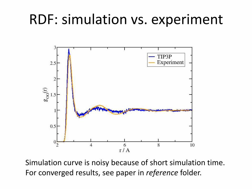
RDF: simulation vs. experiment

Simulation curve is noisy because of short simulation time. For converged results, see paper in reference folder.

Bulk water – mean squared displacement (MSD)

• Work in directory 4

• Task: compute and output the MSD

• Hints:

– Use compute msd

– Assume oxygen MSD = water MSD

– Use fix ave/time to generate output file

• When finished, compare your script and results with content of directory 5

Bulk water – Diffusion

• Work in directory 5 • Diffusion coefficient defined as: D = MSD(t) / 6t with t sufficiently large to get convergence

• MSD data can be post-processed to obtain D: • Check out analysis-tools/msd2diff.py (open with text

editor and see comments for usage instructions) • Example: $ python ../../analysis-tools/msd2diff.py wat.msd 2 3 > wat.diff

• Compare with 5-post

MSD and diffusion

Converged results from paper in reference folder

Water/vapor interface – basic simulation

• Enter directory simulation-interface/1 • Inspect input script • Notice how the change_box command is used to

increase z dimension and create water layers separated by vacuum layers

• Run: $ lammps < in.liquid-vapor • Inspect output • Visualize:

– Directly (.jpg, .mpg) – With VMD (.lammpstrj) Pregenerated visuals available in viz subdirectory

Water surface tension

• Work in directory 1/ • Task: modify input script to compute and output the

surface tension of the water-vacuum system in units of mN/m (milliNewton/meter)

• Surface tension = Lz * [ Pz - ( Px + Py ) / 2 ] / 2 • Hints:

– Use equal-style variables – Average with fix ave/time – Define conversion factors between LAMMPS units and

required output units

• When finished, compare your script and results with content of directory 2/

Water number density profile

• Work in directory 2/

• Task: modify input script to compute and output the number density profile across the water-vacuum interface

• Hints: – Use fix ave/spatial with appropriate keywords

– Compute individual profiles for H and O

• When finished, compare your script and results with content of directory 3/

Water mass density profile

• Work in directory 3/ • Task: post-process H and O number density

profiles to obtain total H2O mass density profile • Hints:

– Use ../../analysis-tools/numDens2massDens.py (open file with text editor and see comments about usage)

– Compute individual profiles for H and O – To get total profile, see ../../analysis-

tools/sumProfile.py

• When finished, compare your results with content of directory 3-post/

Mass density profile across water-vapor interface for various models

Converged results (see paper in reference folder)