interferometric electromagnetic green’s functions ... faculteit... · the wavefield response of...
TRANSCRIPT

Geophys. J. Int. (2007) 169, 60–80 doi: 10.1111/j.1365-246X.2006.03296.xG
JIG
eom
agne
tism
,ro
ckm
agne
tism
and
pala
eom
agne
tism
Interferometric electromagnetic Green’s functions representationsusing propagation invariants
Evert Slob, Deyan Draganov and Kees WapenaarDepartment of Geotechnology, Mijnbouwstraat 120, 2628 RX, Delft, the Netherlands. E-mail: [email protected]
Accepted 2006 November 13. Received 2006 August 17; in original form 2006 March 11
S U M M A R YCreating new responses from cross-correlations of responses measured at different locations isknown as interferometry. Each newly created response represents the field measured at one ofthe receiver locations as if there were a source at the other. Here, we formulate electromagneticinterferometric Green’s functions representations in open configurations. There are in principleno restrictions on the heterogeneity and anisotropy of the medium inside or outside the domain.Time-correlation type formulations rely on conservation of total wave energy and they cannotbe used for media showing relaxation of some form in a straightforward way. Time-convolutiontype propagation invariants are independent of the medium relaxation mechanisms and theycan be used for interferometry by cross-correlating a measured response with the time-reverseof another response. This type of interferometry can only be formulated in the configurationwith one receiver outside the domain. For time-convolution interferometry no restrictions onthe medium heterogeneity, anisotropy or relaxation mechanisms are made. For these interfero-metric formulations to be of practical use, the main simplification is to make a high-frequencyapproximation for the normal derivative in the source coordinate. These approximations of theexact result lead to two different types of errors. We discuss the causes and consequences ofthese errors and illustrate them with numerical examples.
Key words: electromagnetism, interferometry, Green’s function retrieval.
1 I N T RO D U C T I O N
Claerbout (1968) showed that the autocorrelation of an acoustic transmission response recorded in a 1-D configuration at the pressure-free
surface yields the reflection response. Weaver & Lobkis (2001) showed that the autocorrelation function of an acoustic wavefield response is
the wavefield response of a direct pulse-echo experiment in a 3-D configuration. The condition is that the wavefield is diffuse, which in their
case was generated by thermal noise. Based on the diffusivity of the wavefield, many authors showed similar results also for cross-correlations
in open and closed configurations (Lobkis & Weaver 2001; Campillo & Paul 2003; van Tiggelen 2003; Snieder 2004; Roux et al. 2005; Shapiro
et al. 2005). Essentially, Claerbout and Weaver and Lobkis showed the same result, but Claerbout showed it for a 1-D configuration and did
not need a diffuse wavefield. Later it was shown (Wapenaar et al. 2002; Derode et al. 2003) that Claerbout’s principle could be extended to
arbitrary 3-D media.
Wave propagation invariants have been used in acoustic, elastic and electromagnetic wave propagation problems as point of departure
for direct and inverse modelling as well as for imaging (Haines 1988; Kennett et al. 1990; Koketsu et al. 1991; Takenaka et al. 1993). Time-
convolution and time-correlation type reciprocity theorems form two important formulations of propagation invariants (Gangi 1970; Fokkema
& van den Berg 1993; de Hoop 1995; Achenbach 2003). Recently, a novel interpretation of the reciprocity theorem of the time-correlation
type allowed to show that the elastic Green’s function of an arbitrary heterogeneous and anisotropic medium with a pressure-free surface can
be recovered from cross-correlations of particle velocity recordings at two different locations at the pressure-free surface (Wapenaar 2004).
Exact and approximate representations were obtained in terms of correlations of point source responses at these two different locations, where
the sources lie on a semi-closed boundary surface. In this semi-open configuration, the resulting Green’s function represents the total elastic
earth reflection response of a source located at one of the two recording stations, while the receiver is located at the other recording station.
Similar acoustic results were obtained in open systems (Weaver & Lobkis 2004).
Here, we derive interferometric representations of electromagnetic Green’s functions in open configurations for both non-conductive and
conductive media. For exploration geophysics the Earth is probed, hence we restrict ourselves to electromagnetic open configurations. With
the sources located on a closed boundary, interferometric techniques rely on conservation of total wave energy. Then cross-correlation type
techniques have limited use for recordings of wave phenomena where a substantial part of the wave energy is converted into heat and cannot
be used for recordings of electromagnetic diffusive fields or electric potential fields due to stationary currents. For GPR applied to shallow
60 C© 2007 The Authors
Journal compilation C© 2007 RAS
Representations for EM interferometry 61
subsurface investigations, some energy is always converted into heat. We show that if the energy loss factor is not high the kinematics of the
Green’s function are recovered correctly. When the loss factor increases near the boundary sources some artefacts can occur in the form of
spurious time-symmetric events, although the kinematics of all desired arrivals are correct. For electromagnetic waves in conductive media or
media with relaxation, wave energy is dissipated, while for diffusive electromagnetic fields and stationary currents the wave energy is zero.
We show here that for these types of applications exact Green’s function representations can be obtained by convolving two recordings at
two different locations using the reciprocity theorem of the time-convolution type. Hence we extend the notion of interferometry introduced
by Schuster (2001) to include generating new responses from correlation of a signal with a time-reversed signal, which is represented by a
time-convolution. For both types of electromagnetic interferometry we make simplifications to modify the representations such that they can
be used for interferometry. We discuss the effects due to the simplifying assumptions and due to the presence of absorption and illustrate these
discussions with numerical examples at the end of the paper.
2 F O R M U L AT I O N O F L O C A L R E C I P RO C I T Y
For electromagnetic problems we use the electric field vector E(x, t) in (V m−1), the magnetic field vector H (x, t) in (A m−1), the external
source volume densities of electric and magnetic currents, {Je(x, t), Jm(x, t)} in (A m−2) and (V m−2), respectively. The medium parameters
are electric permittivity εkr(x) in [s(�m)−1], electric conductivity σ ekr(x, t) in [(�m)−1], magnetic permeability μ j p(x) in (�sm−1) and the
magnetic conductivity σ mjp(x, t) in (�m−1). Note that we have defined the electric permittivity and the magnetic permeability as functions of
position only. This is no restriction because the time dependence of these medium parameters can be incorporated in the electric and magnetic
conductivities, respectively. That is what we assume here.
We define the time-Fourier transform of a space-time dependent quantity as
E(x, ω) =∫ ∞
t=0
exp(− jωt)E(x, t) dt, (1)
where j is the imaginary unit and ω denotes angular frequency.
In the space-frequency domain Maxwell’s equations in matter are given by
−εkmj∂m H j + [σ e
kr + jωεkr
]Er = − J e
k, (2)
ε jmr∂m Er + [σ m
jp + jωμ j p
]H p = − J m
j , (3)
where ∂m denotes partial differentiation with respect to the coordinate x m and ε kmj is the antisymmetric tensor of rank three, ε kmj = 1 when
kmj = {123, 231, 312}, ε kmj = −1 when kmj = {132, 213, 321}, while ε kmj = 0 otherwise. We use Einstein’s summation convention for
repeated lower case Latin subscripts in the range from 1 to 3. To arrive at the time-convolution type reciprocity theorem, also known as
Lorentz’ reciprocity theorem (Harrington 1961), we consider the interaction quantity
∂mεmkj (Ek,A H j,B − Ek,B H j,A), (4)
where the subscripts A and B are used to distinguish two independent electromagnetic experiments (states). The local electromagnetic
reciprocity theorem of the time-convolution type is obtained by substituting both Maxwell’s equations, eqs (2) and (3), for the two states Aand B into the interaction quantity of eq. (4). For reciprocal media, which implies that the medium parameters in the two states are the same,
εkr,A(x) = εrk,B(x), σ ekr,A(x, ω) = σ e
rk,B(x, ω), (5)
μ j p,A(x) = μpj,B(x), σ mjp,A(x, ω) = σ m
pj,B(x, ω), (6)
this results in
∂mεmkj (Ek,A H j,B − Ek,B H j,A) = J er,A Er,B − J e
r,B Er,A − J mp,A H p,B + J m
p,B H p,A. (7)
In following sections we apply this local reciprocity theorem to a bounded domain.
For the time-correlation type reciprocity theorem we need the complex conjugate of Maxwell’s equations
−εkmj∂m H ∗j + [
σ e∗kr − jωεkr
]E∗
r = − J e∗k , (8)
ε jmr∂m E∗r + [
σ m∗j p − jωμ j p
]H ∗
p = − J m∗j , (9)
where the asterisk denotes complex conjugation. The corresponding interaction quantity is given by
∂mεmkj
(E∗
k,A H j,B + Ek,B H ∗j,A
), (10)
upon taking state A as the time-reversed state (Bojarski 1983). The local electromagnetic reciprocity theorem of the time-correlation type is
obtained by substituting both Maxwell’s equations, eqs (2) and (3), for state B and the time reversed Maxwell’s equations, eqs (8) and (9), for
state A into the interaction quantity of eq. (10). For reciprocal media this results in
−∂mεmkj
(E∗
k,A H j,B + Ek,B H ∗j,A
) = 2H ∗j,A�{
σ mjp
}H p,B + 2E∗
k,A�{σ e
kr
}Er,B
+ J e∗r,A Er,B + J e
r,B E∗r,A + J m∗
p,A H p,B + J mp,B H ∗
p,A, (11)
where �{F} denotes real part of F . In following sections, we apply this local reciprocity theorem to a bounded domain.
C© 2007 The Authors, GJI, 169, 60–80
Journal compilation C© 2007 RAS
62 E. Slob, D. Draganov and K. Wapenaar
3 C O R R E L AT I O N - T Y P E E L E C T RO M A G N E T I C G R E E N ’ S F U N C T I O N
R E P R E S E N TAT I O N S
We start with the global form of the reciprocity theorem of the time-correlation type for the situation applied to the domain ID with closed
boundary ∂ID, which has a unique outward pointing unit normal nm . Without loss of generality in the relaxation mechanisms, we have assumed
that they are all contained in the electric and magnetic conductivity functions. We have assumed reciprocal media and the heterogeneities are
not restricted to occur only inside the domain ID, but may extend over the whole space. Hence, we find an integral reciprocity theorem by
integrating eq. (11) over the domain ID and applying Gauss’ divergence theorem to the integral containing the interaction quantity. This leads
to∮x∈∂ID
nmεmkj
(E∗
k,A H j,B + Ek,B H ∗j,A
)d2x = −2
∫x∈ID
[H ∗
j,A�{σ m
jp
}H p,B + E∗
k,A�{σ e
kr
}Er,B
]d3x
−∫
x∈ID
[( J e
r,A)∗ Er,B + J ek,B E∗
k,A + J mj,B H ∗
j,A + (J m
p,A
)∗H p,B
]d3x. (12)
Eq. (12) is the global reciprocity theorem of the time-correlation type as only products of quantities and complex conjugate quantities occur,
which leads to correlations of these quantities in the time domain. For a more detailed discussion on reciprocity relations, see de Hoop (1995).
One observation worth mentioning is that loss factors inside ID occur only in the first integral on the right-hand side of eq. (12). Various
choices of the sources in the two states lead to exact expressions for the Green’s function in terms of cross-correlations of observed electric
wavefields at the observation points x A and x B due to sources on the closed boundary surface ∂ID.
Let us now focus on the situation where there are no relaxation phenomena and no conductivities inside ID. Then, the first integral in the
right-hand side of eq. (12) vanishes. To localize the electric field receiver at locations x A and x B we specify the artificial point sources for the
source volume densities of the electric current type in both states as
J ek,A = δkrδ(x − xA), (13)
J ek,B = δkpδ(x − xB), (14)
while the magnetic current sources are taken zero everywhere. Using spatial and temporal point sources, we can express the electric field
strengths due to electric current sources in terms of the corresponding Green’s function for heterogeneous anisotropic media. We specify the
electric and magnetic fields due to a point source of electric current at position x = x′, in terms of the Green’s functions as
Ek(x, ω) = G E J e
kr (x, x′, ω) = G E J e
rk (x′, x, ω), (15)
H j (x, ω) = G H J e
jr (x, x′, ω) = −G E J m
r j (x′, x, ω), (16)
which express the source–receiver reciprocity relations for Green’s functions (de Hoop 1995). The terms G E J e, G E J m
represent the electric
field impulse response due to a source of the electric and magnetic current type, respectively, while the term G H J erepresents the magnetic
field impulse response due to a source of the electric current type. Substitution of eqs (13), (15) and (16) in eqs (2) and (3), and eliminating
the magnetic field Green’s function shows that G E J e
rs (x, xA, ω) obeys the following wave equation
εkmp∂mμ−1pj ε jnr∂n G E J e
rs − ω2εkr G E J e
rs = −jωδ(x − xA)δks, (17)
while the magnetic field Green’s function due to an electric current source can be directly obtained from the second Maxwell equation as
G H J e
rs (x, xA, ω) = −(jωμrk)−1εkmp∂m G E J e
ps (x, xA, ω). (18)
Depending on the choices for the receiver locations, x A and x B , being inside or outside ID, electric field Green’s function representations
are obtained. The first choice is to take both points inside the domain ID. Substitution of the electric and magnetic field expressions in terms
of the Green’s functions of eqs (15) and (16) into eq. (12) with zero conductivities leads to
2�{G E J e
kr (xA, xB, ω)} =
∮x∈∂ID
(εmpj nm
{G E J e
kp (xA, x, ω)}∗{
G E J m
r j (xB, x, ω)} + εmpj nm
{G E J m
k j (xA, x, ω)}∗{
G E J e
r p (xB, x, ω)})
d2x, (19)
where we have used the source–receiver reciprocity relations for the Green’s functions. Hence, by taking both observation points inside the
domain ID we obtain a representation for the real part of the Green’s function. This is sufficient because it represents the Fourier transform
of the superposition of the time domain Green’s function plus its time-reversed version, which do not overlap except at t = 0. The choice of
the domain ID is arbitrary as long as both observation points x A and x B lie inside the domain. The representation shows that the electric field
at location x A due to an electric current source at x B is obtained by cross-correlating electric field observations at x A and x B due to electric
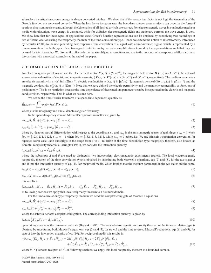
and magnetic current sources at the surface, and integrating over all points x on the boundary ∂ID as depicted in Fig. 1. From this equation it
follows that, in theory, it is possible to construct the exact electric field Green’s function due to an electric current source for any heterogeneous
anisotropic medium from vector product cross-correlations of point source electric field observations at two locations inside the domain ID.
This is the electromagnetic equivalent of the acoustic and elastic Green’s function representations for open configurations given in Wapenaar
& Fokkema (2006). Eq. (19) forms the basis for radar wave interferometry as is discussed in a later section.
C© 2007 The Authors, GJI, 169, 60–80
Journal compilation C© 2007 RAS
Representations for EM interferometry 63
Figure 1. The real part of the frequency domain Green’s function G E J e
kr (xA, xB , ω) can be obtained from cross-correlations of particular combinations of
observations at the locations x A and x B both located inside the domain ID, and summing over all source locations x along the boundary ∂ID. The ray paths
depicted here merely serve for illustration, while they do represent the full electromagnetic wave response of any inhomogeneous and anisotropic medium
inside and outside the domain ID.
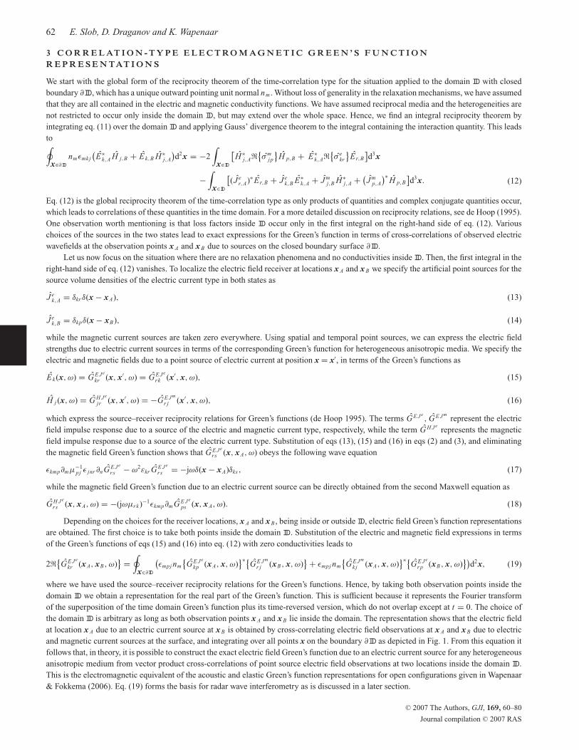
Figure 2. The Green’s function G E J e
kr (xA, xB , ω) can be obtained from cross-correlations of particular combinations of observations at the locations x A located
inside the domain ID and x B located outside the domain ID, and summing over all source locations x along the boundary ∂ID. The ray paths depicted here
merely serve for illustration, while they do represent the full electromagnetic wave response of any inhomogeneous and anisotropic medium inside and outside
the domain ID.
The second choice is to take xA ∈ ID while xB �∈ {ID ∪ ∂ID}, then eq. (12) reduces to
G E J e
kr (xA, xB, ω) =∮
x∈∂ID
(εmpj nm
{G E J e
kp (xA, x, ω)}∗{
G E J m
r j (xB, x, ω)} + εmpj nm
{G E J m
k j (xA, x, ω)}∗{
G E J e
r p (xB, x, ω)})
d2x. (20)
This expression is new and is an exact representation for the electric field received at x A inside the domain ID due to an electric current source
located at x B outside the domain ID in terms of cross-correlations of observed electric wavefields at the observation points x A and x B due to
electric and magnetic current sources on the surface, and integrated over all source positions on the closed boundary ∂ID; see Fig. 2. From
this equation it follows that in theory it is possible to construct the exact electric field Green’s function due to an electric current source from
vector product cross-correlations of electric field observations at a location inside and a location outside the domain ID. Obviously, the same
positions can be localized for magnetic field receivers by choosing artificial non-zero magnetic current sources in both states and zero electric
current sources at the points x A and x B , respectively. This will then result in equivalent exact expressions for the real part of, or the total,
magnetic field Green’s function due to a source of the magnetic current type, G H J m
jp . The cross-coupled Green’s functions can be obtained
directly from Maxwell’s equations and one of the two Green’s functions mentioned above. A third choice would be to take both observation
points outside the domain ID ∪ ∂ID but that would lead to a vanishing contribution of the surface integral.
For both representations for the electric field Green’s functions no assumptions have been made on the heterogeneity and anisotropy
inside and outside the domain ID except that there are no loss and relaxation mechanisms inside ID. As such these equations are sufficient and
suitable to compute the Green’s functions from point sources in x B to point receivers in x A by correlating pre-computed Green’s functions
from source points on the closed surface to the points x A and x B . An example how this can lead to efficient modelling schemes can be found
C© 2007 The Authors, GJI, 169, 60–80
Journal compilation C© 2007 RAS
64 E. Slob, D. Draganov and K. Wapenaar
in van Manen et al. (2005) who used the acoustic equivalent of eq. (19) for computing acoustic Green’s functions of arbitrarily heterogeneous
media.
Since correlation type representations rely on the absence of wave energy dissipation, which is not realistic for most electromagnetic
geophysical methods, we also investigate the possibilities of starting from the convolution type reciprocity relation.
4 C O N V O L U T I O N - T Y P E E L E C T RO M A G N E T I C G R E E N ’ S F U N C T I O N
R E P R E S E N TAT I O N S
To allow for relaxation phenomena and non-zero electric and magnetic conduction currents we now consider the reciprocity theorem of the
time-convolution type. Considering reciprocal media again in the two states, we apply eq. (7) to a domain ID and use Gauss’divergence theorem
in the integral containing the interaction quantity∮x∈∂ID
nmεmkj (Ek,A H j,B − Ek,B H j,A)d2x =∫
x∈ID
(J e
r,A Er,B − J ek,B Ek,A + J m
j,B H j,A − J mp,A H p,B
)d3x. (21)
Note that in the convolution type representations the relaxation and loss mechanisms do not occur in the expression for reciprocal media
and hence we do not have to assume that the media are lossless. This is a strong advantage of the convolution type representations over the
correlation type. All representations that we derive here based on the convolution type reciprocity theorem are in principle valid for wavefields,
diffusion fields, potential fields and flow fields, all fields considered linear. In our analysis we restrict ourselves to the electromagnetic and
stationary electric fields, which apply to ground penetrating radar (GPR), transient and frequency domain electromagnetic methods, including
magneto-telluric methods and seabed logging, as well as geo-electric methods and encompass, therefore, the full electromagnetic spectrum
used in geophysical exploration.
In case both source locations are outside ID ∪ ∂ID or inside ID the boundary integral vanishes (Bojarski 1983). When one of the source
locations is outside ID ∪ ∂ID and the other is inside ID, then we can again derive an expression for the electromagnetic Green’s function for
the electric field. To localize the recording positions we specify artificial point sources for the source volume densities of the electric current
type in both states as J ek,{A,B} = δkrδ(x − xA,B), while the magnetic current sources are taken zero everywhere. The choice for the location of
the recording positions is to take xA ∈ ID while xB �∈ {ID ∪ ∂ID}, then for arbitrary source directions eq. (21) reduces to
G E J e
kr (xA, xB, ω) = −∮
x∈∂ID
εmpj nm
[G E J e
kp (xA, x, ω)G E J m
r j (xB, x, ω) − G E J m
k j (xA, x, ω)G E J e
r p (xB, x, ω)]d2x. (22)
This is an exact and new representation for the electric field Green’s function for a point receiver in x A due to an electric current point source
in x B in terms of vector product cross-convolutions of impulsive electric field responses observed at the observation points x A and x B due to
tangential electric and magnetic point sources on the boundary ∂ID and integrating over all source locations on the closed boundary surface
∂ID. Possible applications of eq. (22) for electromagnetic interferometry will be investigated in the next section.
5 M O D I F I C AT I O N S F O R E M I N T E R F E RO M E T RY
To turn eqs (19), (20) and (22) into a form that can be used in laboratory and field applications the representations should be modified to
include non impulsive sources. Secondly, in their present forms both electric and magnetic current sources occur, which implies they should
be available for all source positions on the boundary. A possible complication is that the representations contain sums of correlations or
convolutions, which implies that the responses at receiver locations x A and x B of each source location on the boundary surface should be
measured separately. This is not a complication under laboratory conditions where we have full control over the source actions and locations.
In a field measurement situation each field can only be recorded separately and then the two fields can be correlated or convolved. Then
the formulation is only useful when the sources are transients and well separated in time. First we modify the representations such that only
electric current sources are required on the boundary. Then further simplifications are introduced for practical sources, transient and noise
sources where possible.
5.1 Radar wave interferometry
We assume again lossless media for radar wave interferometry that can be used for GPR applications and deal first with the presence of
both electric and magnetic current sources and modify the representations such that they can be used in controlled measurement situations
with only electric current sources. We return to the reciprocity relation of eq. (12) and assume that in the neighbourhood of the boundary
surface the medium is isotropic and homogeneous. In our present situation of a relaxation free medium with frequency independent medium
parameters and zero conductivity, we do not yet specify the receiver locations and rewrite eq. (12) in terms of electric fields only, by substituting
H j = −(jωμ)−1ε jmr∂m Er , as
1
jωμ
∮x∈∂ID
nmεmkj
[E∗
k,A(ε jnr∂n Er,B) − Ek,B(ε jnr∂n E∗r,A)
]d2x =
∫x∈ID
[(J e
r,A
)∗Er,B + J e
k,B E∗k,A
]d3x. (23)
The electric current source terms in the right-hand side of eq. (23) are used to localize the receivers at x A and x B . We first concentrate on the
left-hand side of the equation and assume that the receiver locations will be specified either inside ID or outside the domain ID ∪ ∂ID. Then
C© 2007 The Authors, GJI, 169, 60–80
Journal compilation C© 2007 RAS

Representations for EM interferometry 65
under the assumption of local isotropy and homogeneity in the neighbourhood of the closed boundary surface, ∂ID, using Stokes’ curl theorem
and the fact that the electric field is divergence free in a homogeneous isotropic medium it is shown in the Appendix that the left-hand side
can be rewritten in terms of time correlations of the electric field and normal derivatives of the electric field. This results in
1
jωμ
∮x∈∂ID
(E∗
k,Anm∂m Ek,B − Er,Bnm∂m E∗r,A
)d2x =
∫x∈ID
[(J e
r,A
)∗Er,B + J e
k,B E∗k,A
]d3x.
(24)
Making our two choices for the localization of the receivers we find
2�{G E J e
kr (xA, xB, ω)} = 1
jωμ
∮x∈∂ID
({G E J e
k j (xA, x, ω)}∗
nm∂m
{G E J e
r j (xB, x, ω)} − {
nm∂m G E J e
kp (xA, x, ω)}∗{
G E J e
r p (xB, x, ω)})
d2x, (25)
when both xA ∈ ID and xB ∈ ID, while
G E J e
kr (xA, xB, ω) = 1
jωμ
∮x∈∂ID
({G E J e
k j (xA, x, ω)}∗
nm∂m
{G E J e
r j (xB, x, ω)} − {
nm∂m G E J e
kp (xA, x, ω)}∗{
G E J e
r p (xB, x, ω)})
d2x, (26)
when xA ∈ ID and xB �∈ {ID ∪ ∂ID}. In eq. (25) contributions from source points located on the surface for which the total travel time to x A
is larger than to x B will produce events for negative times and lead to the time-reversed part of the Green’s function when summed over all
these sources. On the other hand, contributions from source points located on the surface for which the total travel time to x A is smaller than
to x B will produce events for positive times and lead to the causal part of the Green’s function when summed over all these sources. In eq. (26)
contributions that produce events for negative times lead to zero when summed over all these source locations, while those for positive times
lead to the causal Green’s function when summed over all the sources. In both situations specific events occur for a particular source position
on the boundary that is cancelled by a contribution of another source position or several source positions. We use this property in the next
section where we simplify the integrand further for practical applications. Eqs (25) and (26) are simpler than eqs (19) and (20) for modelling
in the sense that now only a single Green’s function needs to be computed for all source points on the closed boundary surface, but at the cost
of adding a derivative. In the next section, we find suitable approximations for the derivative.
5.2 General electromagnetic interferometry
For more general media with electromagnetic relaxation and non-zero conductivities we cannot use cross-correlation type techniques but need
the cross-convolution type approach. Applying the same analysis, as used for the derivation of eqs (25) and (26), eq. (22) leads to
G E J e
kr (xA, xB, ω) = − 1
jωμ
∮x∈∂ID
({G E J e
k j (xA, x, ω)}nm∂m
{G E J e
r j (xB, x, ω)} − {
nm∂m G E J e
kp (xA, x, ω)}{
G E J e
r p (xB, x, ω)})
d2x, (27)
when xA ∈ ID and xB �∈ {ID ∪ ∂ID}. To arrive at this representation we have made the same assumption of homogeneity and isotropy in
the neighbourhood of the sources on the boundary surface. Again we have reduced the need for electric and magnetic current sources to
only electric current sources at the expense of adding a normal derivative acting on the source coordinate. In eq. (27) the causal part of the
Green’s function is obtained in terms of cross-convolutions. Irrespective of the difference in travel times from the boundary to either x A or
x B , contributions from all source points located on the boundary surface will produce events for positive times and lead to the causal Green’s
function when summed over all these source locations. For a particular source position all events that are not part of the Green’s function are
cancelled by contributions from other source locations.
In the next section, we investigate further simplifications of all three representations by making suitable approximations for the nor-
mal derivative to allow practical applications using transient and mutually uncorrelated noise sources, but first we illustrate the derived
representations of eqs (25), (26) and (27) with a simple example for mutual comparison and to elucidate their differences.
5.3 Numerical example
Here, we give a graphical illustration of eqs (25), (26) and (27) by taking a 2D example with sources lying on a circle with a radius of 1.20 m
and two receivers. For eq. (25) we put receivers at x A = [0, 0.6] m and x B = [0, −0.6] m, see Fig. 3. Fig. 4(a) shows the time domain
equivalent of the integrand of eq. (25) for each source location in a correlation gather. In a correlation gather we show the contribution of each
source position, x, on the boundary as a separate trace. In this example the source position is given in polar coordinates (φ, r = 1.2 m). It is
observed that sources in the neighbourhood of the stationary point at 90o, for which x A is in between the source point and x B , contribute to
the causal result, while the source points in the neighbourhood of the opposite stationary point at 270o contribute to the time-reversed result,
see Snieder et al. (2006) for a detailed stationary phase analysis. The sum of all traces multiplied with rdφ is shown in Fig. 4(b) and represents
the left-hand side of eq. (25).
For the situation that x B is outside the domain ID we leave the receiver location x A unchanged and put x B = [0, 1.8] m such that the
distance between the two receivers is the same as in the first situation, see Fig. 5. The stationary points, are therefore, unchanged at 90◦ and
270◦ but now the sum of integrands should produce the full Green’s function in the frequency domain, which is equivalent to the causal part
only of the time domain Green’s function. From Fig. 6(a) we observe that this is indeed the case. For the correlation result the stationary
point at 270◦ determines the Green’s function, while the stationary point at 90◦ has a vanishing contribution as is clearly observed in the
final causal response shown in Fig. 6(b). This can be understood from the generalized ray paths in the neighbourhood of the stationary points
and the associated travel times to both receiver locations x A and x B . We conclude that only inward travelling waves contribute to the result.
C© 2007 The Authors, GJI, 169, 60–80
Journal compilation C© 2007 RAS

66 E. Slob, D. Draganov and K. Wapenaar
φ
xB
xA
+
+
Figure 3. Two receivers in a homogeneous medium with a number of sources on a circle enclosing both receiver locations. The Green’s function is reconstructed
using eq. (25).
0 45 90 135 180 225 270 315 360–5
–4
–3
–2
–1
0
1
2
3
4
5
φ
time
[ns]
–5
–4
–3
–2
–1
0
1
2
3
4
5
tim
e [ns]
(a) (b)
Figure 4. Correlation gather (a) as a time domain illustration of the integrand of eq. (25). The causal contribution comes from the stationary point at 90◦,
while the anticausal contribution comes from the stationary point at 270◦. The sum over all sources is depicted in (b).
In this particular example the total traveltime in the correlation gather for rays coming from the stationary point at 90◦ is zero because the
distances from the boundary surface to x A and x B are the same. Similarly, for the convolution method the integrand of eq. (27) shows the
Green’s function is obtained from the contribution at the stationary point at 90◦ since then the total traveltime corresponds to the travel time
from x A to x B , for all other points on the boundary the total traveltime of the integrand is larger, as can be seen in Fig. 6(c), and lead to a
vanishing result when the integrand is summed over all source locations as shown in Fig. 6(d). We conclude that the inward travelling waves
recorded at the point inside ID interact with the outward travelling waves recorded at the point outside ID. It can be seen that the amplitude of
the cross-convolution result from source locations away from the stationary point for the convolution method falls off much faster than the
cross-correlation amplitudes for similar source locations in the correlation method. Note that the time scales are different in the final results
shown in Fig. 6(b) and 6(d) due to the different time windows of the correlation and convolution gathers.
From this simple example we can also understand why the non-zero conductivities would affect the correlation type results and not
the convolution type results. In both situations there is a stationary point from which the major contributions come. In the correlation type
representation the travel paths from points in the neighbourhood of the stationary point to x A is traversed by waves that are recorded in both
points. The result is a multiplication of two functions that both suffer from energy loss and lead to squared attenuation in the result, while the
C© 2007 The Authors, GJI, 169, 60–80
Journal compilation C© 2007 RAS

Representations for EM interferometry 67
φ
xB
xA
+
+
Figure 5. Two receivers in a homogeneous medium with a number of sources on a circle enclosing only one receiver location. The Green’s function is
reconstructed using eq. (26).
travel times are subtracted. In the end result the arrival time is correct but the amplitude is not. In the convolution representation the major
contributions come from points near the stationary point that is located such that the travel path to x A goes through the medium inside ID,
while the path to x B is only outside the medium and hence does not suffer from loss terms. In the end result all energy losses are handled
correctly and the travel times are added, leading to the correct travel time.
6 S I M P L I F I C AT I O N S F O R P R A C T I C A L A P P L I C AT I O N S
The presence of the normal derivative in the representations complicates the use of physical sources. To change the representations such that
they can be used in physical measurements we need to simplify the integrands and find approximations for the derivatives. To facilitate this
analysis we simplify the configuration to a domain with horizontal boundaries at x 3 = x 3;1 in the upper half-space and at x 3 = x 3;2 in the lower
half-space; at both boundaries sources are located, see Fig. 7. The unit normal of the top boundary points in the negative x3-direction, while
the unit normal of the bottom boundary points in the positive x3-direction. Note that the positive x3-direction is called the downward direction.
Hence, waves travelling in the positive x3-direction are called downgoing waves and the half-space x 3 > x 3;2 is called the lower half-space.
Both flat surfaces are of infinite extent and the closing cylindrical boundary at infinity has no contribution to the result (Wapenaar et al. 1989).
The domain sandwiched between these two planes can have medium parameters that are arbitrary functions of position and frequency. The
numbers given in the figure are used for illustrative purposes and used in the next section. Both half-spaces are assumed homogeneous and
isotropic, they are allowed to have different constant values for the electric permittivity and magnetic permeability for eqs (25), (26) and (27) to
be valid. Additionally, eq. (27) is still valid when the electric and magnetic conductivities are non-zero and possibly frequency dependent. The
conductivity of all medium parameters is neglected when we use correlation type interferometric representations. This configuration works
for controlled experiments and also applies to practical geophysical electromagnetic exploration methods where measurements are taken in
the air at or above the surface.
6.1 Correlation type interferometry with both receivers inside ID
Using the configuration of Fig. 7 in eq. (25) we start with
2�{G E J e
kr (xA, xB, ω)} = − 1
jωμ1
∫xT ∈IR2
x3=x3;1
({G E J e
k j (xA, x, ω)}∗
∂3
{G E J e
r j (xB, x, ω)} − {
∂3G E J e
kp (xA, x, ω)}∗{
G E J e
r p (xB, x, ω)})
d2xT
+ 1
jωμ2
∫xT ∈IR2
x3=x3;2
({G E J e
k j (xA, x, ω)}∗
∂3
{G E J e
r j (xB, x, ω)} − {
∂3G E J e
kp (xA, x, ω)}∗{
G E J e
r p (xB, x, ω)})
d2xT , (28)
when both xA ∈ ID and xB ∈ ID, while xT = {x 1, x 2} and x = {xT , x 3;1,2}. Waves travelling from the boundary in the direction of the unit
normal, hence away from the domain ID do not return to ID and are not recorded. Waves travelling in the opposite direction of the unit normal
do contribute to the final result. Using Parseval’s relation in eq. (28) we directly see that for propagating waves the first term under the first
C© 2007 The Authors, GJI, 169, 60–80
Journal compilation C© 2007 RAS

68 E. Slob, D. Draganov and K. Wapenaar
0 45 90 135 180 225 270 315 360–0.5
0
0.5
1
1.5
2
2.5
3
3.5
4
4.5
5
φ
time
[ns]
–0.5
0
0.5
1
1.5
2
2.5
3
3.5
4
4.5
5
tim
e [ns]
(a) (b)
0 45 90 135 180 225 270 315 360
4
6
8
10
12
14
16
φ
time
[ns]
4
6
8
10
12
14
16
tim
e [ns]
(c) (d)
Figure 6. Correlation gather (a) and convolution gather (c) as a time domain illustration of the integrand of eqs (26) and (27), respectively. The configuration
is depicted in Fig. 5. The sum over all sources are given for correlation (b) and convolution (d) types of interferometry. For correlation the causal contribution
comes from the stationary point at 270◦, while the stationary point at 90◦ gives a vanishing contribution. For convolution the causal contribution comes from
the stationary point at 90◦, while the stationary point at 270◦ gives a vanishing contribution.
integral on the right-hand side of eq. (28) is the same as the second term but with opposite sign. This is true for both boundaries, see Wapenaar
& Haime (1990) for a more detailed analysis of a similar surface integral for elastic wavefields. We therefore, simplify eq. (28) to
�{G E J e
kr (xA, xB, ω)} ≈ 1
jωμ1
∫xT ∈IR2
x3=x3;1
{∂3G E J e
k j (xA, x, ω)}∗{
G E J e
r j (xB, x, ω)}d2xT
− 1
jωμ2
∫xT ∈IR2
x3=x3;2
{∂3G E J e
k j (xA, x, ω)}∗{
G E J e
r j (xB, x, ω)}d2xT , (29)
when both xA ∈ ID and xB ∈ ID. We have used the approximate sign because we have neglected the contributions from evanescent waves.
We now simplify this result further by assuming that generalized rays that leave the surface perpendicular to the boundary give the major
contribution to the final result, hence we approximate the derivative on boundary source coordinate by
∂3G E Jk j (xA, x, ω)
∣∣x3=x3;1,2
≈ ±jω
c1
G E Jk j (xA, x, ω)
∣∣∣∣x3=x3;1,2
, (30)
C© 2007 The Authors, GJI, 169, 60–80
Journal compilation C© 2007 RAS

Representations for EM interferometry 69
Figure 7. Configuration for the 2D examples, with a three layer medium and with zero and non-zero values for the electric conductivity to investigate the
effects of conductivity in cross-correlation interferometry methods.
where the plus-sign is used for the top boundary and the minus-sign for the bottom boundary (Wapenaar et al. 2005). The wave velocities in
the upper and lower half-space are c1 = (ε1μ1)−1/2, c2 = (ε2μ2)−1/2, respectively. Substituting eq. (30) in eq. (29) leads to
�{G E J e
kr (xA, xB, ω)} ≈ − 1
μ1c1
∫xT ∈IR2
x3=x3;1
{G E J e
k j (xA, x, ω)}∗{
G E J e
r j (xB, x, ω)}d2xT
− 1
μ2c2
∫xT ∈IR2
x3=x3;2
{G E J e
k j (xA, x, ω)}∗{
G E J e
r j (xB, x, ω)}d2xT , (31)
when both xA ∈ ID and xB ∈ ID. Using the approximation of eq. (30) in eq. (29) is rather accurate for the bottom boundary in the situation
where there is a decreasing velocity structure with increasing depth, which is usually the case. For contributions from the top boudary sources,
which lead to waves that travel almost horizontally from x B to x A the largest errors are expected. In general, the approximation can lead to
severe amplitude errors and possibly phase errors. Amplitudes of events in the correlation gather are differently affected depending on the
boundary source location. As discussed above, events in the correlation gather that are not part of the Green’s function are cancelled in the
exact representation when summed over all sources. Hence, events in the approximate correlation gather that should cancel due to destructive
interference when summing over all traces in the gather, can end up in the final trace due to incomplete interference. Still, all desired events
are recovered at correct times, for which reason eq. (31) is considered acceptable for electromagnetic interferometry.
6.2 Transient sources
In situations where we have control over the sources, such as in the laboratory, we can modify eq. (31) to incorporate the time signatures of
the sources. To this end we define electric wavefield recordings at the receiver locations x A and x B as
Eobsk j (xA,B, x, ω) = G E J e
k j (xA,B, x, ω)s( j)(x, ω), (32)
where s( j)(x, ω) denotes the source frequency spectrum in the x j -direction at position x, which can be different for each direction and for
each source position. The power spectrum of the sources is defined as
S( j)(x, ω) = s( j)∗(x, ω)s( j)(x, ω). (33)
Using these definitions in eq. (31) we find
�{G E J e
kr (xA, xB, ω)}
S0(ω) ≈ −∫
xT ∈IR2
x3=x3;1
F ( j)1 (x, ω)
{Eobs
k j (xA, x, ω)}∗{
Eobsr j (xB, x, ω)
}d2xT
−∫
xT ∈IR2
x3=x3;2
F ( j)2 (x, ω)
{Eobs
k j (xA, x, ω)}∗{
Eobsr j (xB, x, ω)
}d2xT , (34)
when both xA ∈ ID and xB ∈ ID. Here S0 is some arbitrarily chosen desired power spectrum, while the shaping filters F ( j) are defined as
F ( j)1,2(x, ω) = Y1,2 S0(ω)
S( j)(x, ω), (35)
C© 2007 The Authors, GJI, 169, 60–80
Journal compilation C© 2007 RAS
70 E. Slob, D. Draganov and K. Wapenaar
where Y 1 = 1/(μ1c1) and Y 2 = 1/(μ2c2) are the plane wave admittances. This choice allows a different source signature for each source
direction and for each source position along the boundaries. This expression can be used in practical applications when all sources are excited
separated in time such that for each source position a full recording can be made. The presence of the shaping filter implies that the source
signature is known. These can be natural sources as long as the above requirement of independent measurements is fulfilled. In this way
we obtain independent measurements for which a correlation gather can be constructed, which, under favourable conditions, also allows
for the identification of spurious events in case of conductive media or due to the high-frequency approximation. It is noted that for GPR
measurements present technology uses low-speed samplers and the time trace is built up by digitizing a single time sample for each excitation
of the transmitter antenna, known as subsampling. Real time sampling is required if we have no control over the sources. In principle, present
technology allows the use of real time sampling in GPR systems with a highest frequency content of 1 GHz as Analogue-to-Digital Converters
(ADC) in the GHz range exist and are used in instrumentation, but not in present commercially available GPR systems. Higher frequency
ADC’s exist (above 20 GHz), which would open up the whole GPR bandwidth, but the number of bits is insufficient and problems with phase
distortions in the higher frequencies prevent these ADC’s to be used in present instrumentation. In controlled source experiments, where we
can use low-frequency samplers, these problems do not exist.
6.3 Uncorrelated noise sources
For laboratory applications independent measurements are achievable, but in natural environments it will be difficult to satisfy the requirement
of independent measurements at each source location and for each source direction. Here, we show that this requirement is dropped when we
have mutually uncorrelated noise sources. We assume noise sources N j (x, ω) that are mutually uncorrelated in the different directions and in
position. When at each surface we have a constant power spectrum S such that 〈N ∗j (x, ω), N p(x′, ω)〉 = Y δ j pδ(x − x′)S(ω), where Y is the
plane wave admittance Y = 1/(μ1c1) for the top interface and Y = 1/(μ2c2) for the bottom interface, we find
�{G E J e
kr (xA, xB, ω)}
S(ω) ≈ −⟨{Eobs
k (xA, ω)}∗
Eobsr (xB, ω)
⟩, (36)
where the observed electric wavefields are given by
Eobsk (xA,B, ω) =
∫xT ∈IR2
x3={x3;1∪x3;2}G E J e
k j (xA,B, x, ω)N j (x, ω) d2xT . (37)
The spatial average in eq. (36) is taken over several realizations of the source distributions, indicated by 〈·〉 in the right-hand side of eq. (36).
The presence of the power spectrum S indicates that the retrieved Green’s function is weighted with the square of the amplitude spectrum of
the noise source and a band limited amplitude bandwidth will result in a smaller bandwidth in the final result. The time domain equivalent is
given by∫ ∞
t ′=−∞
{G E J e
kr (xA, xB, −t ′) + G E J e
kr (xA, xB, t ′)}
S(t − t ′) dt ′ ≈ −2
⟨∫ ∞
t ′=−∞Eobs
k (xA, t ′)Eobsr (xB, t + t ′) dt ′
⟩, (38)
for xA ∈ ID, xB ∈ ID, and expresses that the cross-correlation of electric field measurements at two locations yields the electric field Green’s
function and its time-reversed counterpart between those two locations convolved with the autocorrelation of the noise sources. This result
in eq. (34) is the electromagnetic equivalent of the elastic result in Wapenaar (2004). The advantage here compared to eq. (34) is that all
sources act simultaneously, avoiding the need for separate measurements. Its success depends on the adequacy of the constant power spectrum
assumption, because no shaping filter correction can be applied. Also here the problem for field applications is the limited frequency bandwidth
that can be sampled in real time, essential for noise source applications.
Similar expressions can be found for the cross-correlation and cross-convolution representations in the configuration where one receiver
is outside, ID.
7 E X A M P L E S
Applications of the representations derived here for geophysical electric and electromagnetic exploration methods can be found in forward
modelling, imaging using passive recordings (coherent radiometry) and in inverse modelling. Here, we work out a 2-D example for GPR.
In the usual GPR acquisition configuration we use two parallel broad-side antennas which reduce to a TE-mode acquisition set up in a 2D
setting. We assume that there are several TE-mode line sources of electromagnetic fields in the air and below the bottom interface, and that
these sources lie on a straight line, see Fig. 7. The two observation points are located just above the ground surface as a model for acquisition
with ground coupled antennas. Below the surface a two-layered half plane is considered, each layer being homogeneous. The examples we
show come from this three layered model, upper half-space is air and modelled as free space, the second layer has a thickness of 1 m and
the relative electric permittivity is εr = 9, while the relative electric permittivity of the lower half-space is εr = 16. The upper source level,
x 3;1 is 2 m above the surface where the antennas are placed, while the lower source level, x 3;2, is 2 m below the bottom surface in the lower
half-space. The sources are separated by 10 cm in the horizontal direction and we have used 151 sources spanning a horizontal offset of 7.5 m
in both directions. The source time signature of each boundary source is a second derivative of a Gaussian with a 250 MHz centre frequency.
C© 2007 The Authors, GJI, 169, 60–80
Journal compilation C© 2007 RAS

Representations for EM interferometry 71
xB
Transmitter
xA
Receiver
1
2
3
5
4
Figure 8. The five expected events for antennas at the ground surface. Direct waves through the air (1) and the ground (2), a primary reflection (3) and the
first order multiple (4) and a refracted event (5) when the upgoing wave is incident on the surface at the critical angle.
7.1 Correlation type interferometry with both receivers inside ID
We define the observation points as indicated in Fig. 7 with both points at the ground surface. We first sketch the events we expect to see in
the result. After cross-correlating and integrating over all sources the resulting response is as if the transmitter was at location x B and the
receiver at location x A. Since both antennas are located at the ground surface, we expect direct waves through the air and through the ground
as depicted in Fig. 8. These are known as the direct air wave, event number 1, and the direct ground wave, event number 2. They are not surface
waves but part of the spherical waves that travel upward in the air and downward into the subsurface. Event number 3 represents the reflection
at the subsurface interface and its first order multiple against the ground surface is labelled event number 4. In this sketch we have depicted
a refracted event, event number 5, that is generated because the upgoing multiple event is incident at the critical angle on the ground surface
and travels horizontally in the air along the surface. We use the same numbering of events in the figures that follow for this configuration.
7.1.1 Effects of neglecting the evanescent waves
Fig. 9 shows the separate results from the integral contributions of the top boundary (left), bottom boundary (middle), and their sum (right)
from which the exact result is subtracted. In this example the horizontal distance between the two receivers is 1.5 m. It can be seen that the
major contribution to the final result comes from sources in the lower half-space. The velocity structure used is commonly encountered in
GPR surveys and is responsible for the separation in the contribution from the upper and lower half-space sources. The airwave amplitude
obtained from the bottom boundary is too large and corrected by the result from the top boundary. The effect of neglecting the evanescent
waves is minimal as can be seen in Fig. 9. In the figure the right plot shows the total sum from which the causal directly modelled response is
subtracted. Only for the ground wave some difference is visible. This difference amounts to an error of 5 per cent while the errors for the three
other events are less than 1 per cent. This is understandable from the fact that a horizontally travelling wave just below the ground surface
is only made from the horizontal offsets in the neighbourhood of the stationary point at “infinity”. Fig. 10 shows a CMP gather constructed
from different antennas such that the resulting CMP step size is 10 cm for transmitter and receiver, which is in this case equivalent to a 20 cm
–1 0 1–50
–40
–30
–20
–10
0
10
20
30
40
50
top + bottom
1
2
3
4
–1 0 1–50
–40
–30
–20
–10
0
10
20
30
40
50
top sources
time
[ns]
1
2
3
4
–1 0 1–50
–40
–30
–20
–10
0
10
20
30
40
50
bottom sources
1
2
3
4
Figure 9. Integral contributions from the sources at the top (left plot) and bottom (middle plot) boundaries to the cross-correlation results when evanescent
waves are neglected, while the causal directly modelled response is subtracted from their sum (right plot) for an antenna offset of 1.5 m. The numbered events
are as indicated in Fig. 8.
C© 2007 The Authors, GJI, 169, 60–80
Journal compilation C© 2007 RAS
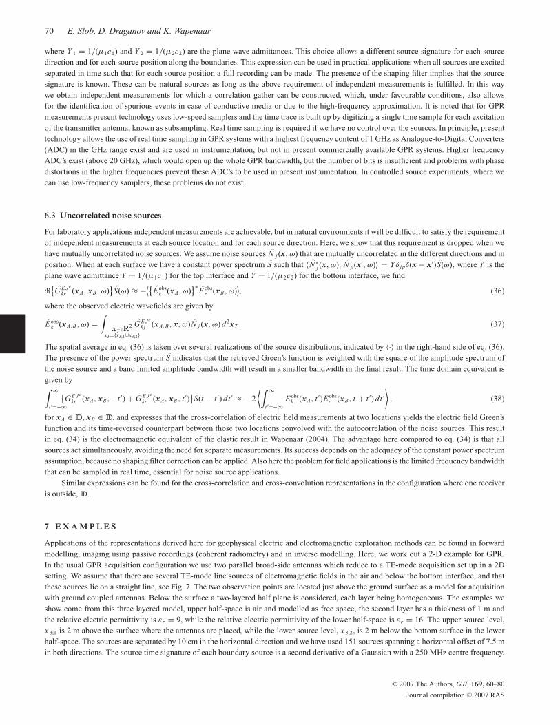
72 E. Slob, D. Draganov and K. Wapenaar
1.5 2 2.5 3 3.5 4 4.5 5 5.5 6 6.5
–80
–60
–40
–20
0
20
40
60
80
offset [m]
time
[ns]
1
2
3
45
Figure 10. CMP constructed from cross-correlation of several antennas, initial offset is 1.5 m and with 20 cm stepsize.
receiver spacing in a shotgather. The full CMP gather is reconstructed including the air and ground waves, the refracted wave (event number
5) at the earth surface as well as the multiple reflections. The unnumbered second order multiple is also visible for larger offsets.
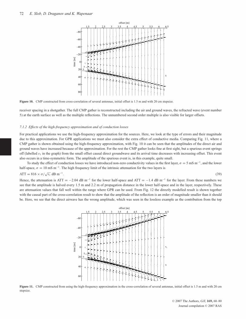
7.1.2 Effects of the high-frequency approximation and of conduction losses
For practical applications we use the high-frequency approximation for the sources. Here, we look at the type of errors and their magnitude
due to this approximation. For GPR applications we must also consider the extra effect of conductive media. Comparing Fig. 11, where a
CMP gather is shown obtained using the high-frequency approximation, with Fig. 10 it can be seen that the amplitudes of the direct air and
ground waves have increased because of the approximation. For the rest the CMP gather looks fine at first sight, but a spurious event springs
off (labelled s1 in the graph) from the small offset causal direct groundwave and its arrival time decreases with increasing offset. This event
also occurs in a time-symmetric form. The amplitude of the spurious event is, in this example, quite small.
To study the effect of conduction losses we have introduced non-zero conductivity values in the first layer, σ = 5 mS m−1, and the lower
half-space, σ = 10 mS m−1. The high frequency limit of the intrinsic attenuation for the two layers is
ATT = 816 × σ/√
εr dB m−1. (39)
Hence, the attenuation is ATT = −2.04 dB m−1 for the lower half-space and ATT = −1.4 dB m−1 for the layer. From these numbers we
see that the amplitude is halved every 1.5 m and 2.2 m of propagation distance in the lower half-space and in the layer, respectively. These
are attenuation values that fall well within the range where GPR can be used. From Fig. 12 the directly modelled result is shown together
with the causal part of the cross-correlation result to show that the amplitude of the reflection is an order of magnitude smaller than it should
be. Here, we see that the direct airwave has the wrong amplitude, which was seen in the lossless example as the contribution from the top
1.5 2 2.5 3 3.5 4 4.5 5 5.5 6 6.5
–60
–40
–20
0
20
40
60
offset [m]
time
[ns]
1
2
s1
3
45
Figure 11. CMP constructed from using the high-frequency approximation in the cross-correlation of several antennas, initial offset is 1.5 m and with 20 cm
stepsize.
C© 2007 The Authors, GJI, 169, 60–80
Journal compilation C© 2007 RAS

Representations for EM interferometry 73
0 5 10 15 20 25 30 35 40 45 50–0.8
–0.6
–0.4
–0.2
0
0.2
0.4
0.6
time [ns]
ampl
itude
exactcross–correlation
Figure 12. Comparison of cross-correlation result in a conductive medium with the directly modelled result of the conductive model at an antenna offset of
1.5 m.
18 20 22 24 26 28 30 32 34–0.8
–0.6
–0.4
–0.2
0
0.2
0.4
0.6
time [ns]
ampl
itude
exactcross–correlation
Figure 13. Close up of the reflection event of Fig. 12 with the amplitude of the cross-correlation result blown up by a factor 13.
boundary. The amplitude loss of the reflections can be understood from the attenuation values. In Fig. 13, we show a close up of the first
order reflection where the cross-correlation result has been multiplied with a factor of 13 to emphasize the phase difference compared to the
exact arrival. The onset of the reflection in the cross-correlation result is clearly advanced while it is correct toward the end of the reflection
event. The event has become more distorted due to the construction from events that have travelled over a larger distance in the layer than
required for the reflection event itself and for contributions from sources in the lower half-space more dispersion is introduced because waves
contributing to the final reflection event have also travelled in the lower half-space. Fig. 14 shows a CMP for the conduction loss situation and
the high-frequency approximation with the same CMP parameters as used in the lossless case, where the difference in recovered amplitude
compared to the result in Fig. 10 is expected. All air related events have a relatively large amplitude, while the near-offset primary and multiple
reflections stand out more in the situation with conduction losses. The spurious event that clearly springs off (event s1 in the figure) from
the direct ground wave arises because the amplitudes of those arrivals, coming from the two parts of the integrands of both source levels, are
different and cause incomplete destructive interference due to the relatively high conductivity in the lower half-space. They always occur in
time-symmetric fashion as we construct the causal part together with its time-reversed equivalent. In the case of small loss factors, which is
the case where wave methods are effective, the spurious events have very small amplitudes and that is favourable for interferometry purposes.
The event is the same as the small amplitude spurious event that was seen in Fig. 11 under the high-frequency approximation, hence, no new
extra spurious events are generated by the presence of conduction losses in this example. Four of the five expected events are visible, be it
with some errors in arrival time and in amplitude, and only the direct ground wave is missing and replaced by a single spurious event (s1)
that is easily identifiable because its arrival time decreases with increasing offsets. From this we conclude that amplitude errors that depend
on source location on the boundary surface lead to slight phase and amplitude errors in desired reflection events and possibly to spurious
C© 2007 The Authors, GJI, 169, 60–80
Journal compilation C© 2007 RAS
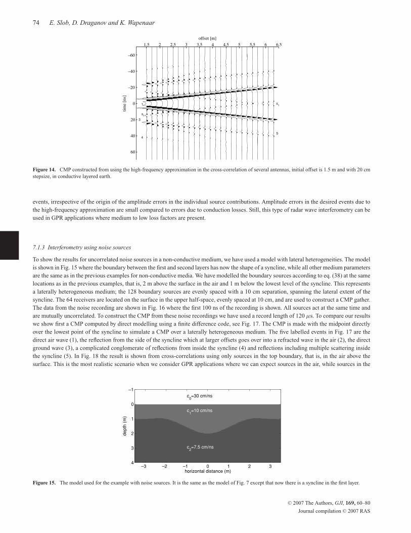
74 E. Slob, D. Draganov and K. Wapenaar
1.5 2 2.5 3 3.5 4 4.5 5 5.5 6 6.5
–60
–40
–20
0
20
40
60
offset [m]
time
[ns]
1
s1
1s
3
45
Figure 14. CMP constructed from using the high-frequency approximation in the cross-correlation of several antennas, initial offset is 1.5 m and with 20 cm
stepsize, in conductive layered earth.
events, irrespective of the origin of the amplitude errors in the individual source contributions. Amplitude errors in the desired events due to
the high-frequency approximation are small compared to errors due to conduction losses. Still, this type of radar wave interferometry can be
used in GPR applications where medium to low loss factors are present.
7.1.3 Interferometry using noise sources
To show the results for uncorrelated noise sources in a non-conductive medium, we have used a model with lateral heterogeneities. The model
is shown in Fig. 15 where the boundary between the first and second layers has now the shape of a syncline, while all other medium parameters
are the same as in the previous examples for non-conductive media. We have modelled the boundary sources according to eq. (38) at the same
locations as in the previous examples, that is, 2 m above the surface in the air and 1 m below the lowest level of the syncline. This represents
a laterally heterogeneous medium; the 128 boundary sources are evenly spaced with a 10 cm separation, spanning the lateral extent of the
syncline. The 64 receivers are located on the surface in the upper half-space, evenly spaced at 10 cm, and are used to construct a CMP gather.
The data from the noise recording are shown in Fig. 16 where the first 100 ns of the recording is shown. All sources act at the same time and
are mutually uncorrelated. To construct the CMP from these noise recordings we have used a record length of 120 μs. To compare our results
we show first a CMP computed by direct modelling using a finite difference code, see Fig. 17. The CMP is made with the midpoint directly
over the lowest point of the syncline to simulate a CMP over a laterally heterogeneous medium. The five labelled events in Fig. 17 are the
direct air wave (1), the reflection from the side of the syncline which at larger offsets goes over into a refracted wave in the air (2), the direct
ground wave (3), a complicated conglomerate of reflections from inside the syncline (4) and reflections including multiple scattering inside
the syncline (5). In Fig. 18 the result is shown from cross-correlations using only sources in the top boundary, that is, in the air above the
surface. This is the most realistic scenario when we consider GPR applications where we can expect sources in the air, while sources in the
horizontal distance (m)
de
pth
(m
)
c0=30 cm/ns
c1=10 cm/ns
c2=7.5 cm/ns
–3 –2 –1 0 1 2 3
–1
0
1
2
3
4
Figure 15. The model used for the example with noise sources. It is the same as the model of Fig. 7 except that now there is a syncline in the first layer.
C© 2007 The Authors, GJI, 169, 60–80
Journal compilation C© 2007 RAS

Representations for EM interferometry 75
–3 –2 –1 0 1 2 30
10
20
30
40
50
60
70
80
90
100
offset [m]
time
[ns]
Figure 16. The first 100 ns of a noise recording from sources in the upper half-space only, with 10 cm distance between the recorders. A two-sided CMP, with
x = 0 as midpoint, can be constructed by autocorrelating the recording at x = 0 and subsequent cross-correlating a recording at negative distance with the
recording at the same positive distance.
–6 –4 –2 0 2 4 60
10
20
30
40
50
60
70
80
90
100
offset [m]
time
[ns]
1
2
3
4
5
Figure 17. A two-sided CMP directly modelled with the midpoint directly over the syncline, with 20 cm stepsize.
–6 –4 –2 0 2 4 60
10
20
30
40
50
60
70
80
90
100
offset [m]
time
[ns]
Figure 18. A two-sided CMP constructed using only noise sources in the upper half-space with the midpoint directly over the syncline, with 20 cm stepsize.
C© 2007 The Authors, GJI, 169, 60–80
Journal compilation C© 2007 RAS

76 E. Slob, D. Draganov and K. Wapenaar
–6 –4 –2 0 2 4 60
10
20
30
40
50
60
70
80
90
100
offset [m]
time
[ns]
Figure 19. A two-sided CMP constructed using noise sources in the upper and lower half-spaces with the midpoint directly over the syncline, with 20 cm
stepsize.
subsurface are far less likely to be present at GPR frequencies. We observe that the CMP contains all important events, (1), (2) and (4), while
the direct ground wave and the multiple scattering effects are almost invisible as they are at the noise level. Some of the complexity of event
(4) is recovered but not completely and certainly not with the correct amplitude. From our analysis using the transient boundary sources this
was expected. Including the contributions from the bottom boundary sources, increases the amplitude of the direct ground wave, while the
accuracy of event (4) has greatly improved within the offset range from −3 to 3 m as can be seen in Fig. 19. This is understandable from the
limited size of the boundary containing the noise sources. Events (2) and (5) are clearly at the noise level and almost invisible.
7.2 Interferometry with one receiver inside and one receiver outside ID
We choose the point x B in the air above the source surface as indicated in Fig. 7, while keeping the rest the same. We first sketch the events
we expect to see in the result in Fig. 20. After cross-correlating and integrating over all sources, the resulting response is as if the transmitter
was at location x B and the receiver at location x A. Since the transmitter antenna is located above the ground surface in the air it gives rise to
the direct wave, event number 1. Event number 2 represents the reflection at the subsurface interface and its first order multiple against the
ground surface is labelled event number 3. We use the same numbering of events in figures that follow for this configuration.
We first look at the the errors made from giving the wrong sign to contributions from waves that leave the top source boundary directly
in the negative x3-direction. The effects can be seen in Fig. 21, where we show the contributions from the top (left plot) and bottom (middle
plot) boundaries, while the exact response is subtracted from their sum in the right plot. We see that five spurious events, labelled s1 to s5,
four occur at negative times and one at positive times (s3). This results from neglecting evanescent waves, leading to slight amplitude errors,
xB
Transmitter
xA
Receiver
1
32
Figure 20. The three expected events for the transmitter antenna above and the receiver antenna at the ground surface.
C© 2007 The Authors, GJI, 169, 60–80
Journal compilation C© 2007 RAS

Representations for EM interferometry 77
–1 0 1–60
–40
–20
0
20
40
60
top + bottom
1
2
3
s1
s2
s3
s4
s5
–1 0 1–60
–40
–20
0
20
40
60
top sources
time
[ns]
1
2
3
s1
s2
s3
s4
s5
–1 0 1–60
–40
–20
0
20
40
60
bottom sources
1
2
3
s1
s2
Figure 21. Contributions from the sources at the top (left) and bottom (middle) boundaries to the cross-correlation results using the correct sign for inward
travelling waves, while in the right plot the causal directly modelled response is subtracted from their sum, at a horizontal antenna offset of 1.5 m and vertical
offset of 4 m.
and from the error we made for the top source level by reducing the integrands to single term. This second error produces events by giving
waves that have travelled upward directly from the sources at the top boundary the wrong sign. These waves are now added to the same waves
from which they should have been subtracted. Spurious events s1 and s2 are present in the contributions from both source surfaces and should
cancel each other, but are now added. The three events s 3, s 4 and s5 are introduced in the contribution from the top boundary alone. Since the
right plot of Fig. 21 has no visible expected events when the exact response is subtracted from the approximate response, we conclude that
neglecting the evanescent waves leads to negligible errors and that the errors introduced by assigning the wrong sign to waves that directly
travel upward from the top source boundary lead to spurious events that all occur before the first desired arrival, which is known. These
properties make this configuration very suitable for interferomtric purposes.
In Fig. 22, we show the result from the same configuration, but now using cross-convolutions of the two recordings. Two spurious events
are present, labelled s1 and s2, because of the sign error that was introduced with the approximation for the waves travelling directly down
from the top boundary before they are recorded at x B . This is problematic since in principle there is no way to tell whether an event in the time
window of interest is physical or unphysical. A way around this problem is to combine correlation- and convolution-type interferometry for
this configuration and from comparing Figs 21 and 22 we see that all unphysical events are easily recognized because they arrive at different
times in the two results, while the physical events arrive of course at the correct times. Secondly, all spurious events vanish due to destructive
interference when the source surface has an irregular shape, which has been demonstrated first by Draganov et al. (2004).
The high-frequency approximations do not lead to new events in either cross-correlation or cross-convolution results. Conductive media
lead in this configuration for cross-correlations results to similar effects that have been discussed in the paragraph with both receivers inside
the domain. Therefore, those results are not presented here.
0 10 20 30 40 50 60 70 80 90 100
–0.6
–0.4
–0.2
0
0.2
0.4
0.6
0.8
time [ns]
am
plit
ud
e
1 s1 2
3 s2
Figure 22. Contributions from the sources at the top boundary to the cross-convolution result using the high-frequency approximation at a horizontal antenna
offset of 1.5 m and vertical offset of 4 m.
C© 2007 The Authors, GJI, 169, 60–80
Journal compilation C© 2007 RAS
78 E. Slob, D. Draganov and K. Wapenaar
8 C O N C L U S I O N S
We have extended known exact interferometric Green’s function representations for acoustic and elastic wavefields to their electromagnetic
equivalents. These representations give the Green’s function terms of cross-correlations of observations made at two locations enclosed by a
boundary containing sources. Similar modifications are presented that are necessary for applications in GPR interferometry. This was possible
in a configuration where the medium outside the domain ID is homogeneous and hence only ingoing waves that leave the source boundary
contribute to the final result and proper approximations can be made for the derivative.
We have derived new exact electromagnetic integral Green’s function representations for a configuration where one observation point
is inside the domain bounded by the surface sources, while the other observation point is outside this domain. For this new configuration,
interferometric Green’s function representations are obtained in terms of cross-correlations and in terms of cross-convolutions of the observed
fields. The cross-convolution representation has the advantage that it remains valid for fields where wave energy is converted into heat or
where wave energy is absent. This occurs for GPR, transient and frequency domain EM and geo-electric applications of electromagnetic
exploration. The disadvantage is that no formulation was found that can be easily used in field exploration because artefacts arrive in the time
window of interest, but combined interpretation with cross-correlation results can be used to identify spurious events in the cross-convolution
results. We have shown that for cross-correlation type interferometry we can find a formulation for the new configuration that can be used
in laboratory and field applications using transient or uncorrelated noise sources. In this new configuration, one receiver is located inside
the domain bounded by the boundary sources, while the other receiver location is outside. For this outside located receiver, both ingoing
and outgoing waves contribute to the final result. In the simplified configuration with flat boundaries in homogeneous half-spaces, this
problem only occurs for the boundary that lies between the two receivers. It is then possible to find a suitable formulation for electromagnetic
interferometry. This is because we can always use a configuration where spurious events, due to the necessary approximations for practical
applicability, can be moved to negative times or at least to times before the first arrival, which is known. The absence of spurious events in
the causal part of the cross-correlation interferometry data can be used to identify spurious events in the cross-convolution interferometry
data. Apart from the occurrence of these identifiable erroneous events, we have shown that there are two other causes of errors in the form
of spurious events. These other two causes of errors occur in the configuration where both observation points are inside the domain and in
the configuration where one observation point is outside the domain. In the high-frequency approximation amplitude errors are made that
change for different source locations on the boundary and consequently can lead to incomplete cancellation of events in the correlation gather
that are not part of the final result. Depending on the configuration, the amplitudes of these spurious events can be negligibly small to large
compared to desired events. The second source of errors is due to the actual presence of wave energy loss mechanisms in cross-correlation
methods. This also leads to amplitude errors that change with the position of the boundary sources and hence can lead to spurious events.
We have shown that if wave energy dominates, which is the case where wave methods work best, these spurious events are quite small. In
case where loss factors are large combined use of cross-correlation and cross-convolution interferometry helps to identify spurious events in
the cross-convolution result and we find the desired events with almost the correct amplitude. These two new interferometry formulations
in the new configuration with one receiver located inside and one outside the domain ID can be used for acoustic and elastic wavefields as
well.
R E F E R E N C E S
Achenbach, J., 2003. Reciprocity in Elastodynamics, Cambridge University
Press, Cambridge, UK.
Bojarski, N., 1983. Generalized reaction principles and reciprocity theorems
for the wave equations, and the relationships between time-advanced and
time-retarded fields., J. Acous. Soc. Am., 74, 281–285.
Campillo, M. & Paul, A., 2003. Longe-range correlations in the diffuse
seismic coda waves, Science, 299, 547–549.
Claerbout, J., 1968. Synthesis of a layered medium from its acoustic trans-
mission response, Geophysics, 33, 264–269.
de Hoop, A., 1995. Handbook of Radiation and Scattering of Waves, Aca-
demic Press, Amsterdam.
Derode, A., Larose, E., Tanter, M., de Rosny, J., Tourin, A., Campilo, M.
& Fink, M., 2003. Recovering the Green’s function from field-field cor-
relations in an open scattering medium(L), JASA, 113, no. 6, 2973–2976,
doi:10.1121/1.1570436.
Draganov, D., Wapenaar, K. & Thorbecke, J., 2004. Passive seismic imag-
ing in the presence of white noise sources, Leading Edge, 23, 889–
892.
Fokkema, J. & van den Berg, P., 1993. Seismic Applications of AcousticReciprocity, Elsevier, Amsterdam.
Gangi, A., 1970. A derivation of the seismic representation theorem using
seismic reciprocity, J. Geophys. Res., 75, 2088–2095.
Haines, A., 1988. Multi-source, multi-receiver synthetic seismograms for
laterally heterogeneous media using f-k domain propagators, Geophys. J.Int., 95, 237–260.
Harrington, R., 1961. Time-Harmonic Electromagnetic Field, McGraw-Hill,
New York.
Kennett, B., Koketsu, K. & Haines, A., 1990. Propagation invariants, re-
flection and transmission in anisotropic, laterally heterogeneous media,
Geophys. J. Int., 103, 95–101.
Koketsu, K., Kennett, B. & Takenaka, H., 1991. 2-D reflectivity method and
symmetric seismograms for irregularly layered structures - II. invariant
embedding approach, Geophys. J. Int., 105, 119–130.
Lobkis, O. & Weaver, R., 2001. On the emergence of the {G}reen’s function
in the correlations of a diffuse field, JASA, 110, 3011–3017.
Roux, P., Sabra, K., Kuperman, W. & Roux, A., 2005. Ambient noise cross
correlation in free space: theoretical approach, JASA, 117, no. 1, 79–84.
Schuster, G., 2001. Theory of daylight/interferometric imaging: tutorial, in
Extended Abstracts of the 63rd Mtg., Eur. Assoc. Geosc. & Eng., p. Paper:
A32.
Shapiro, N., Campillo, M., Stehly, L. & Ritzwoller, M., 2005. High-
resolution surface-wave tomography from ambient seismic noise, Science,307, 1615–1618.
Snieder, R., 2004. Extracting the Green’s function from the correlation of
coda waves: A derivation based on stationary phase, Phys. Rev. E, 69,046 610–1–8, doi:10.1103/PhysRevE.69.046610.
Snieder, R., Wapenaar, K. & Larner, K., 2006. Spurious multiples in seismic
interferometry of primaries, Geophysics, 71, SI 111–SI 124.
C© 2007 The Authors, GJI, 169, 60–80
Journal compilation C© 2007 RAS
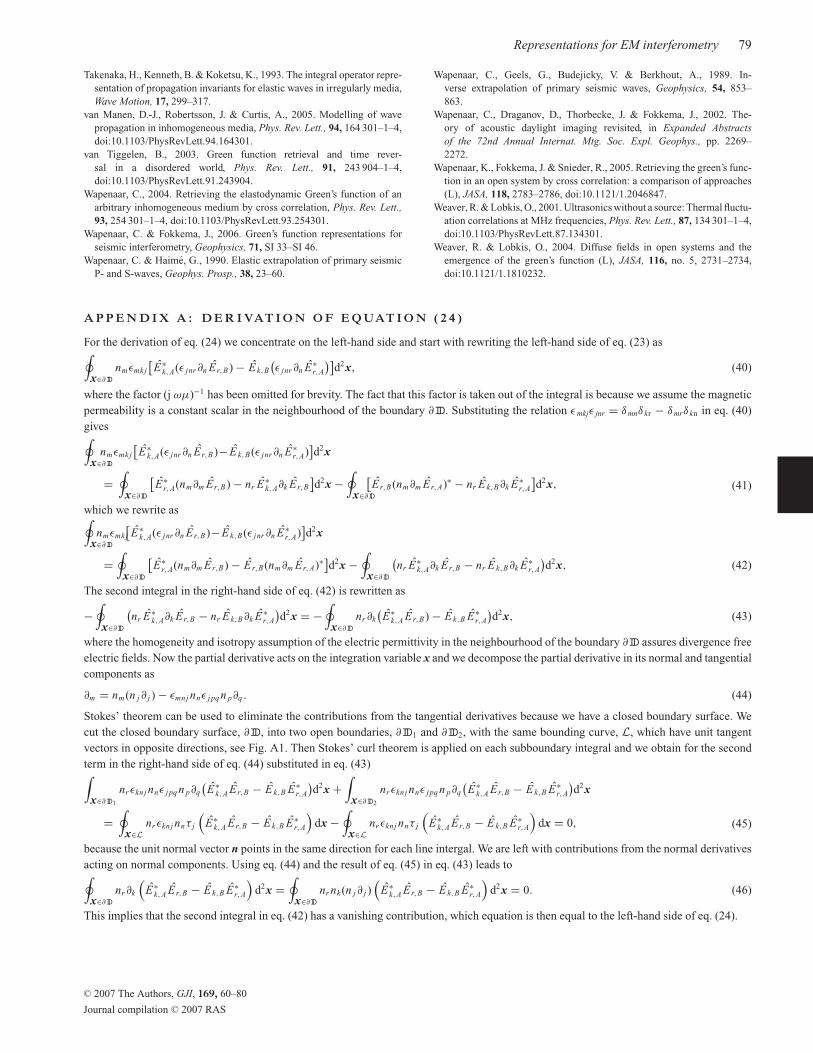
Representations for EM interferometry 79
Takenaka, H., Kenneth, B. & Koketsu, K., 1993. The integral operator repre-
sentation of propagation invariants for elastic waves in irregularly media,
Wave Motion, 17, 299–317.
van Manen, D.-J., Robertsson, J. & Curtis, A., 2005. Modelling of wave
propagation in inhomogeneous media, Phys. Rev. Lett., 94, 164 301–1–4,
doi:10.1103/PhysRevLett.94.164301.
van Tiggelen, B., 2003. Green function retrieval and time rever-
sal in a disordered world, Phys. Rev. Lett., 91, 243 904–1–4,
doi:10.1103/PhysRevLett.91.243904.
Wapenaar, C., 2004. Retrieving the elastodynamic Green’s function of an
arbitrary inhomogeneous medium by cross correlation, Phys. Rev. Lett.,93, 254 301–1–4, doi:10.1103/PhysRevLett.93.254301.
Wapenaar, C. & Fokkema, J., 2006. Green’s function representations for
seismic interferometry, Geophysics, 71, SI 33–SI 46.
Wapenaar, C. & Haime, G., 1990. Elastic extrapolation of primary seismic
P- and S-waves, Geophys. Prosp., 38, 23–60.
Wapenaar, C., Geels, G., Budejicky, V. & Berkhout, A., 1989. In-
verse extrapolation of primary seismic waves, Geophysics, 54, 853–
863.
Wapenaar, C., Draganov, D., Thorbecke, J. & Fokkema, J., 2002. The-
ory of acoustic daylight imaging revisited, in Expanded Abstractsof the 72nd Annual Internat. Mtg. Soc. Expl. Geophys., pp. 2269–
2272.
Wapenaar, K., Fokkema, J. & Snieder, R., 2005. Retrieving the green’s func-
tion in an open system by cross correlation: a comparison of approaches
(L), JASA, 118, 2783–2786, doi:10.1121/1.2046847.
Weaver, R. & Lobkis, O., 2001. Ultrasonics without a source: Thermal fluctu-
ation correlations at MHz frequencies, Phys. Rev. Lett., 87, 134 301–1–4,
doi:10.1103/PhysRevLett.87.134301.
Weaver, R. & Lobkis, O., 2004. Diffuse fields in open systems and the
emergence of the green’s function (L), JASA, 116, no. 5, 2731–2734,
doi:10.1121/1.1810232.
A P P E N D I X A : D E R I VAT I O N O F E Q UAT I O N ( 2 4 )
For the derivation of eq. (24) we concentrate on the left-hand side and start with rewriting the left-hand side of eq. (23) as∮x∈∂ID
nmεmkj
[E∗
k,A(ε jnr∂n Er,B) − Ek,B
(ε jnr∂n E∗
r,A
)]d2x, (40)
where the factor (j ωμ)−1 has been omitted for brevity. The fact that this factor is taken out of the integral is because we assume the magnetic
permeability is a constant scalar in the neighbourhood of the boundary ∂ID. Substituting the relation εmkjε jnr = δmnδkr − δmrδkn in eq. (40)
gives∮x∈∂ID
nmεmkj
[E∗
k,A(ε jnr∂n Er,B)− Ek,B(ε jnr∂n E∗r,A)
]d2x
=∮
x∈∂ID
[E∗
r,A(nm∂m Er,B) − nr E∗k,A∂k Er,B
]d2x −
∮x∈∂ID
[Er,B(nm∂m Er,A)∗ − nr Ek,B∂k E∗
r,A
]d2x, (41)
which we rewrite as∮x∈∂ID
nmεmkj
[E∗
k,A(ε jnr∂n Er,B)− Ek,B(ε jnr∂n E∗r,A)
]d2x
=∮
x∈∂ID
[E∗
r,A(nm∂m Er,B) − Er,B(nm∂m Er,A)∗]d2x −
∮x∈∂ID
(nr E∗
k,A∂k Er,B − nr Ek,B∂k E∗r,A
)d2x, (42)
The second integral in the right-hand side of eq. (42) is rewritten as
−∮
x∈∂ID
(nr E∗
k,A∂k Er,B − nr Ek,B∂k E∗r,A
)d2x = −
∮x∈∂ID
nr∂k
(E∗
k,A Er,B) − Ek,B E∗r,A
)d2x, (43)
where the homogeneity and isotropy assumption of the electric permittivity in the neighbourhood of the boundary ∂ID assures divergence free
electric fields. Now the partial derivative acts on the integration variable x and we decompose the partial derivative in its normal and tangential
components as
∂m = nm(n j∂ j ) − εmnj nnε j pq n p∂q . (44)
Stokes’ theorem can be used to eliminate the contributions from the tangential derivatives because we have a closed boundary surface. We
cut the closed boundary surface, ∂ID, into two open boundaries, ∂ID1 and ∂ID2, with the same bounding curve, L, which have unit tangent
vectors in opposite directions, see Fig. A1. Then Stokes’ curl theorem is applied on each subboundary integral and we obtain for the second
term in the right-hand side of eq. (44) substituted in eq. (43)∫x∈∂ID1
nrεknj nnε j pq n p∂q
(E∗
k,A Er,B − Ek,B E∗r,A
)d2x +
∫x∈∂ID2
nrεknj nnε j pq n p∂q
(E∗
k,A Er,B − Ek,B E∗r,A
)d2x
=∮
x∈Lnrεknj nnτ j
(E∗
k,A Er,B − Ek,B E∗r,A
)dx −
∮x∈L
nrεknj nnτ j
(E∗
k,A Er,B − Ek,B E∗r,A
)dx = 0, (45)
because the unit normal vector n points in the same direction for each line intergal. We are left with contributions from the normal derivatives
acting on normal components. Using eq. (44) and the result of eq. (45) in eq. (43) leads to∮x∈∂ID
nr∂k
(E∗
k,A Er,B − Ek,B E∗r,A
)d2x =
∮x∈∂ID
nr nk(n j∂ j )(
E∗k,A Er,B − Ek,B E∗
r,A
)d2x = 0. (46)
This implies that the second integral in eq. (42) has a vanishing contribution, which equation is then equal to the left-hand side of eq. (24).
C© 2007 The Authors, GJI, 169, 60–80
Journal compilation C© 2007 RAS
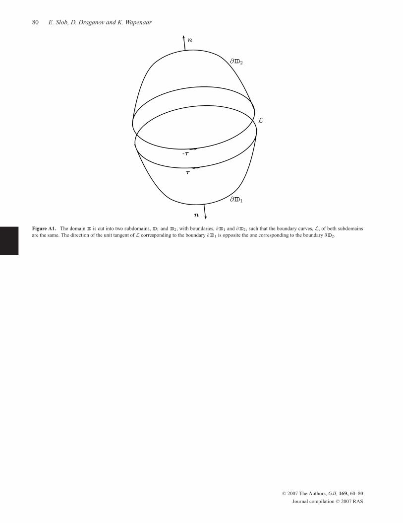
80 E. Slob, D. Draganov and K. Wapenaar
τ
n
∂ID1
L
∂ID2
-τ
n
Figure A1. The domain ID is cut into two subdomains, ID1 and ID2, with boundaries, ∂ID1 and ∂ID2, such that the boundary curves, L, of both subdomains
are the same. The direction of the unit tangent of L corresponding to the boundary ∂ID1 is opposite the one corresponding to the boundary ∂ID2.
C© 2007 The Authors, GJI, 169, 60–80
Journal compilation C© 2007 RAS