intelligent network selection and energy reduction...
TRANSCRIPT

Intelligent Network Selection and EnergyReduction for Mobile Devices
by
Shuo Deng
B.S., Automation, Tsinghua University (2009)
S.M., Computer Science, Massachusetts Institute of Technology (2012)
Submitted to the Department of Electrical Engineering and Computer Science
in partial fulfillment of the requirements for the degree of
Doctor of Philosophy in Computer Science
at the
Massachusetts Institute of Technology
June 2015
c○Massachusetts Institute of Technology 2015. All rights reserved.
Author . . . . . . . . . . . . . . . . . . . . . . . . . . . . . . . . . . . . . . . . . . . . . . . . . . . . . . . . . . . . . . . . . . . . . . . . . . .
Department of Electrical Engineering and Computer Science
May 20, 2015
Certified by . . . . . . . . . . . . . . . . . . . . . . . . . . . . . . . . . . . . . . . . . . . . . . . . . . . . . . . . . . . . . . . . . . . . . . .
Hari Balakrishnan
Professor
Thesis Supervisor
Accepted by . . . . . . . . . . . . . . . . . . . . . . . . . . . . . . . . . . . . . . . . . . . . . . . . . . . . . . . . . . . . . . . . . . . . . .
Leslie A. Kolodziejski
Chair, Department Committee on Graduate Theses


Intelligent Network Selection and EnergyReduction for Mobile Devices
by
Shuo Deng
Submitted to the Department of Electrical Engineering and Computer Science on
May 20, 2015, in partial fulfillment of the requirements for the degree of
Doctor of Philosophy in Computer Science
ABSTRACT
The popularity of mobile devices has stimulated rapid progress in both Wi-Fi and cellular
technologies. Before LTE was widely deployed, Wi-Fi speeds dominated cellular network
speeds. But that is no longer true today. In a study we conducted with a crowd-sourced
measurement tool used by over 1,000 users in 16 countries, we found that 40% of the
time LTE outperforms Wi-Fi, and 75% of the time the difference between LTE and Wi-Fi
throughput is higher than 1 Mbits/s.
Thus, instead of the currently popular “always prefer Wi-Fi” policy, we argue that mo-
bile devices should use the best available combination of networks: Wi-Fi, LTE, or both.
Selecting the best network combination, however, is a challenging problem because: 1)
network conditions vary with both location and time; 2) many network transfers are short,
which means that the decision must be made with low overhead; and, 3) the best choice is
determined not only by best network performance, but also constrained by practical factors
such as monetary cost and battery life.
In this dissertation, we present Delphi, a software controller for network selection on
mobile devices. Delphi makes intelligent network selection decisions according to cur-
rent network conditions and monetary cost concerns, as well as battery-life considerations.
Our experiments show that Delphi reduces application network transfer time by 46% for
web browsing and by 49% for video streaming, compared with Android’s default policy
of always using Wi-Fi when it is available. Delphi can also be configured to achieve high
3

throughput while being energy efficient; in this configuration, it achieves 1.9× the through-
put of Android’s default policy while only consuming 6% more energy.
Delphi improves performance but uses the cellular network more extensively than the
status quo, consuming more energy than before. To address this problem, we develop a
general method to reduce the energy consumption of cellular interfaces on mobile devices.
The key idea is to use the statistics of data transfers to determine the best times at which to
put the radio in different power states. These techniques not only make Delphi more useful
in practice but can be deployed independently without Delphi to improve energy efficiency
for any cellular-network-enabled devices. Experiments show that our techniques reduce
energy consumption by 15% to 60% across various traffic patterns.
Dissertation Supervisor: Hari Balakrishnan
Title: Professor
4

To Xinming and my parents

6

Contents
List of Figures 11
List of Tables 17
Previously Published Material 19
Acknowledgments 21
1 Introduction 23
1.1 Measuring Wi-Fi and Cellular Networks . . . . . . . . . . . . . . . . . . . 25
1.2 Network Selection for Multi-homed Mobile Devices . . . . . . . . . . . . 25
1.3 Reducing the Energy Consumed by the Cellular Interface . . . . . . . . . . 27
1.4 Contributions . . . . . . . . . . . . . . . . . . . . . . . . . . . . . . . . . 28
1.5 Outline . . . . . . . . . . . . . . . . . . . . . . . . . . . . . . . . . . . . 29
2 Measurement Study 31
2.1 Cell vs. Wi-Fi Measurement . . . . . . . . . . . . . . . . . . . . . . . . . 32
2.1.1 Cell vs. Wi-Fi App . . . . . . . . . . . . . . . . . . . . . . . . . . 32
2.1.2 Results . . . . . . . . . . . . . . . . . . . . . . . . . . . . . . . . 34
2.2 MPTCP Measurements . . . . . . . . . . . . . . . . . . . . . . . . . . . . 37
2.2.1 MPTCP Overview . . . . . . . . . . . . . . . . . . . . . . . . . . 37
2.2.2 Measurement Setup . . . . . . . . . . . . . . . . . . . . . . . . . . 38
2.2.3 TCP vs. MPTCP . . . . . . . . . . . . . . . . . . . . . . . . . . . 41
2.2.4 Primary Flow Measurement . . . . . . . . . . . . . . . . . . . . . 44
7

2.2.4.1 MPTCP Throughput Evolution Over Time . . . . . . . . 45
2.2.4.2 MPTCP Throughput as a Function of Flow Size . . . . . 47
2.2.5 Coupled and Decoupled Congestion Control . . . . . . . . . . . . 48
2.2.6 Full-MPTCP and Backup Modes . . . . . . . . . . . . . . . . . . . 51
2.2.6.1 Packet-Level Behavior of Full-MPTCP and Backup Modes 51
2.2.6.2 Energy Efficiency in Backup Mode . . . . . . . . . . . . 53
2.3 Mobile App Traffic Patterns . . . . . . . . . . . . . . . . . . . . . . . . . 55
2.3.1 Record-Replay Tool . . . . . . . . . . . . . . . . . . . . . . . . . 55
2.3.2 Traffic Patterns of Mobile Apps . . . . . . . . . . . . . . . . . . . 56
2.4 Mobile App Replay . . . . . . . . . . . . . . . . . . . . . . . . . . . . . . 56
2.4.1 Short-Flow Dominated App Replay . . . . . . . . . . . . . . . . . 58
2.4.2 Long-flow Dominated App Replay . . . . . . . . . . . . . . . . . . 61
2.5 Related Work . . . . . . . . . . . . . . . . . . . . . . . . . . . . . . . . . 63
2.5.1 Wi-Fi/Cellular Comparison . . . . . . . . . . . . . . . . . . . . . . 63
2.5.2 Multi-Path TCP . . . . . . . . . . . . . . . . . . . . . . . . . . . . 63
2.6 Chapter Summary . . . . . . . . . . . . . . . . . . . . . . . . . . . . . . . 64
3 Delphi: A Controller for Mobile Network Selection 67
3.1 Overview . . . . . . . . . . . . . . . . . . . . . . . . . . . . . . . . . . . 68
3.2 Traffic Profiler . . . . . . . . . . . . . . . . . . . . . . . . . . . . . . . . . 69
3.3 Network Monitor . . . . . . . . . . . . . . . . . . . . . . . . . . . . . . . 70
3.3.1 Network Indicators . . . . . . . . . . . . . . . . . . . . . . . . . . 71
3.3.2 Adaptive Probing . . . . . . . . . . . . . . . . . . . . . . . . . . . 72
3.4 Predictor . . . . . . . . . . . . . . . . . . . . . . . . . . . . . . . . . . . . 75
3.4.1 Regression Tree Prediction Accuracy . . . . . . . . . . . . . . . . 76
3.4.2 Input Error Analysis . . . . . . . . . . . . . . . . . . . . . . . . . 77
3.4.2.1 Traffic Profiler Error . . . . . . . . . . . . . . . . . . . . 78
3.4.2.2 Network Monitor Error . . . . . . . . . . . . . . . . . . 78
3.5 Network Selector . . . . . . . . . . . . . . . . . . . . . . . . . . . . . . . 79
3.5.1 Objective Functions . . . . . . . . . . . . . . . . . . . . . . . . . 79
8

3.5.2 Energy Model . . . . . . . . . . . . . . . . . . . . . . . . . . . . . 80
3.5.3 Selector Performance . . . . . . . . . . . . . . . . . . . . . . . . . 81
3.5.4 System Generalization . . . . . . . . . . . . . . . . . . . . . . . . 85
3.6 Implementation . . . . . . . . . . . . . . . . . . . . . . . . . . . . . . . . 86
3.7 Evaluation . . . . . . . . . . . . . . . . . . . . . . . . . . . . . . . . . . . 88
3.7.1 Delphi Over Emulated Networks . . . . . . . . . . . . . . . . . . . 88
3.7.2 Experiments . . . . . . . . . . . . . . . . . . . . . . . . . . . . . 90
3.7.3 Handling User Mobility . . . . . . . . . . . . . . . . . . . . . . . 91
3.8 Discussion . . . . . . . . . . . . . . . . . . . . . . . . . . . . . . . . . . . 92
3.8.1 Purely Location-Based Algorithm . . . . . . . . . . . . . . . . . . 92
3.8.2 Picking the Recent-Best Choice . . . . . . . . . . . . . . . . . . . 94
3.9 Related Work . . . . . . . . . . . . . . . . . . . . . . . . . . . . . . . . . 95
3.9.1 Mobile Network Selection . . . . . . . . . . . . . . . . . . . . . . 95
3.9.2 Multi-Path TCP . . . . . . . . . . . . . . . . . . . . . . . . . . . . 96
3.9.3 Processor Sharing for Multiple Interfaces . . . . . . . . . . . . . . 96
3.9.4 Roaming Mechanisms . . . . . . . . . . . . . . . . . . . . . . . . 97
3.9.5 Systems and APIs to Exploit Multiple Interfaces . . . . . . . . . . 97
3.10 Chapter Summary . . . . . . . . . . . . . . . . . . . . . . . . . . . . . . . 98
4 Energy Consumption for LTE and 3G 99
4.1 Introduction . . . . . . . . . . . . . . . . . . . . . . . . . . . . . . . . . . 99
4.2 Background . . . . . . . . . . . . . . . . . . . . . . . . . . . . . . . . . . 102
4.2.1 3G/LTE State Machine . . . . . . . . . . . . . . . . . . . . . . . . 102
4.2.2 Energy Consumption . . . . . . . . . . . . . . . . . . . . . . . . . 103
4.3 Design . . . . . . . . . . . . . . . . . . . . . . . . . . . . . . . . . . . . . 105
4.4 MakeIdle Algorithm . . . . . . . . . . . . . . . . . . . . . . . . . . . . . 106
4.4.1 Optimal Decision From Offline Trace Analysis . . . . . . . . . . . 107
4.4.2 Online Prediction . . . . . . . . . . . . . . . . . . . . . . . . . . . 108
4.5 MakeActive Algorithm . . . . . . . . . . . . . . . . . . . . . . . . . . . . 110
4.5.1 Fixed Delay Bound . . . . . . . . . . . . . . . . . . . . . . . . . . 112
9

4.5.2 Learning Algorithm . . . . . . . . . . . . . . . . . . . . . . . . . 112
4.6 Evaluation . . . . . . . . . . . . . . . . . . . . . . . . . . . . . . . . . . . 113
4.6.1 Simulation Setup . . . . . . . . . . . . . . . . . . . . . . . . . . . 113
4.6.2 Comparison of Energy Savings . . . . . . . . . . . . . . . . . . . . 116
4.6.3 MakeIdle Evaluation . . . . . . . . . . . . . . . . . . . . . . . . . 120
4.6.4 MakeActive Evaluation . . . . . . . . . . . . . . . . . . . . . . . . 123
4.6.5 Different Carriers . . . . . . . . . . . . . . . . . . . . . . . . . . . 123
4.6.6 Energy Overhead of Running Algorithms . . . . . . . . . . . . . . 127
4.6.7 Implementation Results . . . . . . . . . . . . . . . . . . . . . . . 128
4.7 Related Work . . . . . . . . . . . . . . . . . . . . . . . . . . . . . . . . . 129
4.7.1 3G Energy Mitigation Strategies . . . . . . . . . . . . . . . . . . . 129
4.7.2 3G Resource Usage Profiling . . . . . . . . . . . . . . . . . . . . . 130
4.7.3 Wi-Fi Power-Saving Algorithms . . . . . . . . . . . . . . . . . . . 130
4.7.4 Power-Saving for Processors . . . . . . . . . . . . . . . . . . . . . 131
4.8 Chapter Summary . . . . . . . . . . . . . . . . . . . . . . . . . . . . . . . 131
5 Conclusion 133
5.1 Contributions . . . . . . . . . . . . . . . . . . . . . . . . . . . . . . . . . 133
5.2 Future Work . . . . . . . . . . . . . . . . . . . . . . . . . . . . . . . . . . 134
A Bank of Experts 135
10

List of Figures
1-1 Energy consumed by the 3G interface. “Data” corresponds to a data trans-
mission; “DCH Timer” and “FACH Timer” are each the energy consumed
with the radio in the idle states specified by the two timers, and “State
Switch” is the energy consumed in switching states. These timers and state
switches are described in §4.2. . . . . . . . . . . . . . . . . . . . . . . . . 27
2-1 Cell vs. Wi-Fi User Interface. . . . . . . . . . . . . . . . . . . . . . . . . . 32
2-2 Cell vs. Wi-Fi: single measurement collection run. . . . . . . . . . . . . . . 33
2-3 CDF of difference between Wi-Fi and LTE throughput. The gray region
shows 42% (uplink) and 35% (downlink) of the data samples whose LTE
throughput is higher than Wi-Fi throughput. . . . . . . . . . . . . . . . . . 36
2-4 CDF of the difference between average Ping RTT with Wi-Fi and LTE. The
gray region shows 20% of the data samples whose LTE RTT is lower than
Wi-Fi RTT. . . . . . . . . . . . . . . . . . . . . . . . . . . . . . . . . . . 36
2-5 Setup of MPTCP measurement. . . . . . . . . . . . . . . . . . . . . . . . 39
2-6 CDF for Wi-Fi and LTE throughput measured using regular TCP at 20
locations (shown as “20-Location”) compared with the CDF in Figure 2-3
(shown as “App Data”). . . . . . . . . . . . . . . . . . . . . . . . . . . . 40
2-7 MPTCP throughput vs single-path TCP throughput at 2 representative loca-
tions. Figure 2-7a shows a case in which MPTCP throughput is lower than
the best throughput of single-path TCP. Figure 2-7b shows a case where
MPTCP throughput (in this case, MPTCP (Wi-Fi, decoupled)) is higher
than that of single-path TCP for large flow sizes. . . . . . . . . . . . . . . . 41
11

2-8 Acknowledged data vs. time for TCP and MPTCP. . . . . . . . . . . . . . 42
2-9 MPTCP sent and acknowledged data sequence number vs. time on sender
and receiver side. . . . . . . . . . . . . . . . . . . . . . . . . . . . . . . . 42
2-10 Acknowledged data vs. time for TCP and MPTCP when initial congestion
control window is 1 MSS. . . . . . . . . . . . . . . . . . . . . . . . . . . . 44
2-11 MPTCP sent and acknowledged data sequence number vs. time on sender
and receiver side, when initial congestion control window is 1 MSS. . . . . 44
2-12 CDF of relative difference between MPTCPLT E and MPTCPWi−Fi, for dif-
ferent flow sizes. The median relative difference for each flow size is: 60%
for 10 KBytes, 49% for 100 KBytes and 28% for 1MByte. Thus, through-
put for smaller flow sizes is more affected by the choice of the network for
the primary subflow. . . . . . . . . . . . . . . . . . . . . . . . . . . . . . 45
2-13 MPTCP throughput over time, measured at a location where LTE had higher
throughput than Wi-Fi had. MPTCP throughput grows faster over time
when using LTE for the primary subflow. . . . . . . . . . . . . . . . . . . 46
2-14 MPTCP throughput over time, measured at a location where Wi-Fi had
higher throughput than LTE had. MPTCP throughput grows faster over
time when using Wi-Fi for the primary subflow. . . . . . . . . . . . . . . . 46
2-15 Absolute throughput difference and relative throughput ratio as a function
of flow size when LTE has higher throughput than Wi-Fi has. . . . . . . . . 47
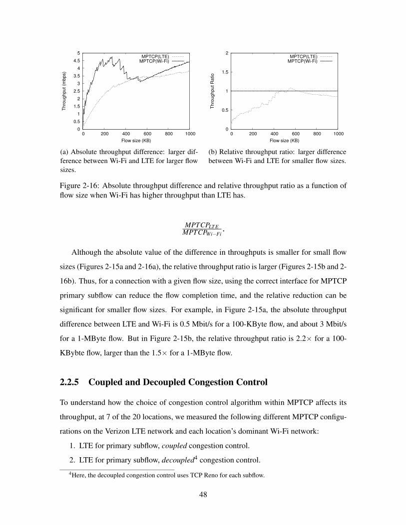
2-16 Absolute throughput difference and relative throughput ratio as a function
of flow size when Wi-Fi has higher throughput than LTE has. . . . . . . . . 48
2-17 CDF of relative difference between MPTCPcoupled and MPTCPdecoupled ,
for different flow sizes. The median relative difference for each flow size:
16% for 10 KBytes, 16% for 100 KBytes and 34% for 1 MByte. Thus,
throughput for larger flow sizes is most affected by the choice of congestion
control. . . . . . . . . . . . . . . . . . . . . . . . . . . . . . . . . . . . . 49
12

2-18 CDF of relative difference using different networks for primary subflow
(labeled as “Network”) vs. using different congestion control algorithms
(labeled as “CC”), across 3 flow sizes. Median values for CC curves are:
16% for “10 KB”, 16% for “100 KB”, and 34% for “1 MB”. Thus, using
different congestion control algorithms has more impact on larger flows.
Median values for Network curves are: 60% for “ 10 KB”, 43% for “100
KB” , and 25% for “1 MB”. Thus, using a different network for the primary
subflow has greater impact on smaller flows. . . . . . . . . . . . . . . . . 50
2-19 Full-MPTCP and Backup modes. . . . . . . . . . . . . . . . . . . . . . . . 52
2-20 Power level for LTE and Wi-Fi when used as non-backup subflow. LTE
has a much higher power level than Wi-Fi in non-backup mode. LTE also
consumes an excessive amount of energy even in backup mode. . . . . . . . 54
2-21 Traffic patterns for app launching and user interacting. Figures 2-21d and 2-
21f show the “long-flow dominated” traffic pattern; the other figures show
the “short-flow dominated” pattern. . . . . . . . . . . . . . . . . . . . . . . 57
2-22 CNN app response time under different network conditions. . . . . . . . . 59
2-23 CNN normalized app response reduction by different oracle schemes. . . . 59
2-24 Dropbox app-response time under different network conditions. . . . . . . 61
2-25 Dropbox normalized app-response reduction by different oracle schemes. . 62
3-1 Delphi design. . . . . . . . . . . . . . . . . . . . . . . . . . . . . . . . . . 68
3-2 Correlation between Wi-Fi/LTE single path TCP throughput and each indi-
cator. . . . . . . . . . . . . . . . . . . . . . . . . . . . . . . . . . . . . . . 72
3-3 As the adaptive probing threshold (x-axis) increases, the number of probing
decreases and the probing error increases. Here the left y-axis shows the
probing frequency, which is the average number of probing in every five
minutes. . . . . . . . . . . . . . . . . . . . . . . . . . . . . . . . . . . . . 74
13

3-4 Relative error when using the regression tree and support vector regression
to learn the flow completion time. The line marked with “Tree” shows the
relative error of the regression tree model. The line with “SVR” shows the
relative error of the support vector regression model. . . . . . . . . . . . . 76
3-5 Relative error when using an empirical flow size number (3 KBytes) to
predict flow completion time. The legends are the actual flow sizes. . . . . 77
3-6 Relative error when using adaptive probing to predict flow completion time. 78
3-7 Megabits per joule and throughput values for different schemes. The black
line shows a frontier of the best median values that can be achieved when
setting α = 1, γ = 0 and changing β from 0 to 5. For each scheme, the
black dot shows the median value and the ellipse shows the 30th and 70th
percentiles. . . . . . . . . . . . . . . . . . . . . . . . . . . . . . . . . . . 82
3-8 Percentage of each network(s) is selected when using different objective
functions. . . . . . . . . . . . . . . . . . . . . . . . . . . . . . . . . . . . 83
3-9 Success rate for different schemes. . . . . . . . . . . . . . . . . . . . . . . 84
3-10 Objective function value normalized by oracle. The histogram shows the
median value; the error bar shows 20th and 80th percentiles. . . . . . . . . 88
3-11 Objective function value normalized by oracle. The histogram shows the
median value; the error bar shows one standard deviation. . . . . . . . . . . 89
3-12 When the mobile device is moving away from an access point, Delphi pre-
dicts that Wi-Fi can be worse than LTE, then it switches to LTE at time
10.5 seconds. MPTCP handover mode switches to LTE when it sees Wi-Fi
loses the IP, which happens at time 41 seconds. . . . . . . . . . . . . . . . 91
3-13 Wi-Fi and LTE download throughput at the same location over 2.5 hours. . 92
3-14 Wi-Fi and LTE download throughput measured indoors and outdoors. The
bar shows the average throughput over 10 measurements; the error bar
shows the standard deviation. . . . . . . . . . . . . . . . . . . . . . . . . . 93
3-15 Throughput normalized by oracle. The histogram shows the median value;
the error bar shows the 20th and 80th percentiles. The bars labeled “Recent-
best” show the results for picking-the-recent-best. . . . . . . . . . . . . . . 94
14

4-1 Energy consumed by the 3G interface. “Data” corresponds to a data trans-
mission; “DCH Timer” and “FACH Timer” are each the energy consumed
with the radio in the idle states specified by the two timers, and “State
Switch” is the energy consumed in switching states. These timers and state
switches are described in §4.2. . . . . . . . . . . . . . . . . . . . . . . . . 101
4-2 Radio Resource Control (RRC) State Machine. . . . . . . . . . . . . . . . 102
4-3 The measured power consumption of the different RRC states. Exact values
can be found in Table 4.2. In these figures the power level for IDLE/RRC_IDLE
is non-zero because of the CPU and LED screen power consumption. . . . 104
4-4 System design. . . . . . . . . . . . . . . . . . . . . . . . . . . . . . . . . 106
4-5 Simplified power model for 3G energy consumption (for an LTE model, t2
equals to zero). . . . . . . . . . . . . . . . . . . . . . . . . . . . . . . . . 107
4-6 If the energy consumed by the picture on the right is less than the one on
the left, then turning the radio to Idle soon after the first transmission will
consume less energy than leaving it on. The energy is easily calculated by
integrating the power profiles over time. . . . . . . . . . . . . . . . . . . . 108
4-7 “Shift” traffic to reduce number of state switches. . . . . . . . . . . . . . . 111
4-8 Simulation energy error for Verizon 3G and LTE networks. . . . . . . . . . 114
4-9 Energy savings for different applications.“4.5-second” sets the inactivity
timer to 4.5 seconds. “95% IAT” uses the 95th percentile of packet inter-
arrival time observed over the entire trace as the inactivity timer. “MakeI-
dle” shows the energy saved by our MakeIdle algorithm. “MakeIdle +Make-
Active Learn” and “MakeIdle +MakeActive Fix” show the energy sav-
ings when running MakeIdle together with two different MakeActive algo-
rithms: learning algorithm and fixed delay bound algorithm. Oracle shows
the maximum achievable energy savings without delaying any traffic. . . . 116
4-10 Energy savings and signaling overhead (number of state switches) across
users in the Verizon 3G network. . . . . . . . . . . . . . . . . . . . . . . . 117
4-11 Energy savings and signaling overhead (number of state switches) across
users in the Verizon LTE network. . . . . . . . . . . . . . . . . . . . . . . 118
15

4-12 False (“FP” short for false positive) and missed switches (“FN” short for
false negative). . . . . . . . . . . . . . . . . . . . . . . . . . . . . . . . . 121
4-13 False (“FP”) and missed switches (“FN”) changes as the number of packets
used to construct distribution ( defined in § 4.4.2) changes. . . . . . . . . . 122
4-14 Waiting time changes in MakeIdle. . . . . . . . . . . . . . . . . . . . . . . 122
4-15 Mean and median delays for traffic bursts using learning algorithm and
fixed delay bound scheme. . . . . . . . . . . . . . . . . . . . . . . . . . . 124
4-16 Delay value changes as the learning proceeds. . . . . . . . . . . . . . . . . 125
4-17 Energy saved for different carrier parameters using different methods. For
MakeIdle, the maximum gain is 67% in the Verizon LTE network. For
MakeIdle+MakeActive, the maximum gain is 75% achieved in Verizon 3G. 126
4-18 Number of state switches (signaling overhead) for different methods di-
vided by number of state switches using the current inactivity timers. . . . 126
4-19 Average power level measured when a Sony Xperia phone was transferring
data with and without MakeIdle enabled. . . . . . . . . . . . . . . . . . . . 128
16

List of Tables
2.1 Geographical coverage and diversity of the crowd-sourced data collected
from 16 countries using Cell vs. Wi-Fi, ordered by number of runs col-
lected. The last column shows the percentage of runs in which LTE’s
throughput is higher than Wi-Fi’s throughput. . . . . . . . . . . . . . . . . 35
2.2 Locations where MPTCP measurements were conducted. . . . . . . . . . . 40
3.1 HTTP transaction data lengths for the Alexa top 500 sites. 84% of the
transfer lengths are predictable by the Traffic Profiler. . . . . . . . . . . . . 69
3.2 Network indicators monitored by Delphi. . . . . . . . . . . . . . . . . . . 71
3.3 Overhead for one occurrence of active probing. The delay values are the
median value across all measurement data collected at 22 locations. The
energy values are measured in an indoor setting. The cellular energy values
do not contain tail-energy [26]. . . . . . . . . . . . . . . . . . . . . . . . . 73
3.4 Power level measurement for Wi-Fi and LTE in a indoor setting. The Wi-
Fi power is measured when the mobile device is associated with an AP
deployed inside the building. The LTE power is measured when the mobile
device is connected to Verizon LTE network. . . . . . . . . . . . . . . . . 81
3.5 Median values for Max(S), Max(S/E) and Wi-Fi as shown in Figure 3-7. . . 83
3.6 Median values for throughput and energy efficiency when testing different
models at new locations. . . . . . . . . . . . . . . . . . . . . . . . . . . . 85
17

3.7 Switching delay, averaged across 10 measurements. The switching delay is
defined as the time between an iptable rule-changing command being
issued and a packet transfer occurring on the newly brought-up interface.
The send delay is the delay for the first out-going packet showing up, and
the receive delay is for the first ACK packet coming from the server. . . . . 86
4.1 Average power in mW measured on Galaxy Nexus in Verizon network. The
energy consumed by CPU and screen is subtracted. . . . . . . . . . . . . . 114
4.2 Power and inactivity timer values for different networks. Power values are
in mW; times are in seconds (measured in September 2011). . . . . . . . . 125
4.3 The mean and median session delays brought by MakeIdle for different
carriers (in seconds). . . . . . . . . . . . . . . . . . . . . . . . . . . . . . 125
18

Previously Published Material
This dissertation includes material from the following publications:
1. Shuo Deng, Ravi Netravali, Anirudh Sivaraman, Hari Balakrishnan. “WiFi, LTE, or
Both? Measuring Multi-Homed Wireless Internet Performance”, ACM IMC 2014.
(Chapter 2)
2. Shuo Deng, Anirudh Sivaraman, Hari Balakrishnan. “All Your Network Are Belong
to Us: A Transport Framework for Mobile Network Selection”, HotMobile 2014.
(Chapter 3)
3. Shuo Deng, Alvin Cheung, Sam Madden, Hari Balakrishnan.“Multi-Network Con-
trol Framework for Mobile Applications”, ACM S3 2013. (Chapter 3)
4. Shuo Deng, Anirudh Sivaraman, Hari Balakrishnan. “Delphi: A Software Controller
for Mobile Network Selection”, Submitted for publication. (Chapter 3)
5. Shuo Deng, Hari Balakrishnan. “Traffic-Aware Techniques to Reduce 3G/LTE Wire-
less Energy Consumption”, ACM CoNEXT 2012. (Chapter 4)
The dataset used in Chapters 2 and 3 is available at http://web.mit.edu/
cell-vs-wifi.
19

20

Acknowledgments
I would like to thank my advisor, Hari Balakrishnan, for his guidance and advice in the past
six years, and also for being open-minded and supportive about my career choice. During
these years, I learned much from Hari, including how to tackle new research problems,
pitch ideas, and give presentations. I believe these skills will be valuable not only for my
research but also for my future life, no matter what career path I choose.
I would also like to thank my thesis committee members, Sam Madden and Dina Katabi.
As my academic advisor, Sam has given me guidance not only on graduate courses but
also on research. Dina offered me the opportunity to give practice talks during her group
meeting, and provided valuable feedback.
I would also like to thank my labmates and colleagues. Katrina LaCurts’s dedication
to research has really inspired me. I feel fortunate to have worked with her on her cloud
computing project, from which I learned a great deal about how to conduct research. I
have also worked closely with Alvin Cheung, Anirudh Sivaraman, Ravi Netravali, and
Tiffany Chen. They brought fun, motivation, and relief to my research. I also want to thank
Lenin Ravindranath, Raluca Ada Popa, Keith Winstein, Jonathan Perry, Amy Ousterhout
for giving me valuable feedback and detailed comments on writing papers.
My research has benefited from our collaboration with Foxconn. I feel fortunate to have
worked with Foxconn engineers: Leon Lee, Ethan Kuo, Edward Lu, and Sigma Huang.
Without their hard work and expertise in network engineering, it was hard to imagine how
I could deploy my algorithms on commercial devices.
My parents have supported me unconditionally throughout my life. Their life stories
taught me to always be focused and determined and keep inner peace. I thank my grand-
father and grandmother for being supportive of my study abroad. Special thanks goes to
21

my husband, Xinming Chen, who has been my 24/7 technical and emotional support all
through graduate school, and who gave up a cozy life in China to end our long-distance
relationship and start a new page of life together in the United States.
22

Chapter 1
Introduction
By the end of 2014, the number of mobile-connected devices had exceeded the world’s
population [74]. The popularity of these devices has stimulated further rapid progress in
both Wi-Fi and cellular technology. Now the 802.11 standard provides a Wi-Fi link rate as
high as 1 Gbps [1]. Cellular networks have advanced from EDGE to 3G to LTE, or 4G,
with peak downlink speed also in the order of 1 Gbps [2].
Despite all these high-speed wireless technologies being widely deployed, the lack of an
intelligent network selection mechanism prevents mobile device users from fully exploiting
available network resources. Today’s mobile operating systems typically hard-code the
decision of which network to use when confronted with multiple choices. If the user has
previously associated with an available Wi-Fi network, the mobile device uses that over a
cellular option. This choice often leads to frustrating results. For example, when walking
outdoors, users often find their device connecting to a Wi-Fi access point inside a building
and experience poor performance when the right answer is to use the cellular network.
Even inside homes and buildings, a static choice is not always the best: there are rooms
where the Wi-Fi network might be much slower than the cellular network, depending on
other users, time of day, and other factors. Thus, network selection for mobile devices
needs to be done dynamically since Wi-Fi and cellular networks are not evenly distributed,
either spatially or temporally.
Moreover, in practice, users care not just about performance but also about the monetary
cost of using wireless networks as well as battery life. These factors increase the difficulty
23

of the network-selection problem. Indeed, one reason many current mobile devices always
prefer Wi-Fi over cellular is because Wi-Fi is generally free, whereas cellular is generally
not. However, for some users with a monthly cellular data plan, the downside of being too
conservative with using cellular networks is that they may end up paying a subscription
fee every month while using little of their data plan budget. Meanwhile, the economics
of cellular data plans are changing. After being offered beginning in 2007, “unlimited”
plans were halted in 2011 by several carriers (although pre-existing users could hold on to
them). Since 2013, however, unlimited plans have made a resurgence, especially in Tier-2
operators, where 45% of the users have such plans today [74]. In addition, an increasing
number of major app providers like Facebook, Google, and WhatsApp, have proposed and
are deploying “zero rating” plans so that mobile device users will not be charged when
these apps generate cellular traffic [83]. Thus, an intelligent network selection mechanism
should be able to cope with different monetary cost models.
Another major concern is energy consumption. It is well known that the cellular ra-
dio consumes significant amounts of energy; on the iPhone 6 Plus, for example, the stated
internet-use time is “up to 12 hours on 3G or LTE” (i.e., when the 3G radio is on and in
“typical” use) and the talk-time is “up to 24 hours”.1 On the Nexus 5, the equivalent num-
bers are “up to 7 hours on LTE for internet-use” and “up to 17 hours for talk time”2. Thus,
to improve overall user experience, an intelligent network selection mechanism should not
merely aim for increasing the network speed.
This dissertation begins with a measurement study analyzing the network performance
of mobile devices in the real world. This measurement study also shows that significant
improvements may be achieved if network selection is done properly. Then, we present
Delphi, a software controller for network selection on mobile devices. Delphi makes intel-
ligent network selection decisions according to current network conditions, monetary cost
concerns, as well as battery level. Delphi’s design is based on data collected during the
measurement study. We also implement Delphi and show that it can improve network per-
formance in real-world experiments. Finally, we take a deeper look into the causes of high
1http://www.apple.com/iphone-6/specs/2https://support.google.com/nexus/answer/3467463?hl=en&ref_topic=
3415523
24

energy consumption when a mobile device uses the cellular network, and develop software
solutions to improve the energy-efficiency of cellular interfaces.
1.1 Measuring Wi-Fi and Cellular Networks
We conducted a set of measurements using a crowd-sourced network measurement tool as
well as with controlled experiments (§2). The conclusions from this measurement study
are as follows:
1. Over 73% of the time, the throughput of one of the networks was higher than the
other by at least 1 Mbit/s. When the throughput difference was at least 1 Mbit/s,
LTE/4G had higher throughput 56% of the time, and Wi-Fi 44% of the time; that is,
it was roughly split down the middle. The throughput differentials depended on the
transfer size, due to the dynamics of TCP congestion control.
2. Over 83% of the time, the round-trip latency of one of the networks was higher than
the other by at least 100 ms.
3. Multipath TCP (MPTCP) [77], which uses multiple interfaces whenever possible,
did not always out-perform single-path TCP connections. A key factor in MPTCP’s
performance was the choice of primary subflow, that is, the network on which the
initial connection and data transfer is done. This choice has a strong effect on the
throughput, particularly for short and medium-sized transfers.
These conclusions left a key question open: How do we design a practical software
module for mobile devices to select the best network for applications? This question is
important for both single-path and multi-path TCP transfers.
1.2 Network Selection for Multi-homed Mobile Devices
To answer this question, we designed Delphi (§3), a mobile software controller that helps
mobile applications select the best network among available choices for their data transfers.
Our starting point is from the perspective of users and applications rather than the trans-
port layer or the network. Depending on the objectives of interest, Delphi makes different
25

decisions about which network to use and in what order.
We consider three objectives (though the framework handles other objectives as well):
1. minimize the time to complete an application-level transfer (the ratio of transfer size
to transfer throughput);
2. minimize the energy per byte of the transfer, which usually (but not always) entails
picking only one network; and
3. minimize the monetary cost per byte of the transfer.
Delphi provides a framework to optimize these and similar objectives. This problem
is challenging because the answer changes with time, and depends on location and user
movement.
Delphi has four components:
1. Network Performance Predictor estimates the latency and throughput of different
networks by running a machine-learning predictor using features obtained from the
Network Monitor.
2. The Network Monitor uses passive observations of wireless network properties such
as the Received Signal Strength Indicator (RSSI) and channel quality, lightweight
active probes, and an adaptive method that uses active probes only when passive
indicators suggest a significant change in conditions.
3. Traffic Profiler provides an estimate of the length of transfers; this component is
required because throughput depends on the size of the transfer.
4. Network Selector uses network performance predictions, transfer lengths, and the
specified objectives for application transfers to determine which network to use for
each transfer.
Our evaluation shows that:
1. In our simulations over traces collected from 22 locations, Delphi improved the me-
dian throughput by 2.1× compared with always using Wi-Fi, the default policy on
Android devices today. Delphi can also be configured to achieve high throughput
while being energy-efficient; in this mode, it achieves 1.9× throughput while con-
suming only 6% more energy compared with Android’s default policy.
2. When running with unmodified applications, Delphi reduces applications’ network
26

transfer time by 46% for web browsing and by 49% for video streaming, compared
with Android’s default policy.
3. Delphi is also proactive in switching networks when the device is moving. It can de-
tect that the network that is currently in use is performing worse than the alternatives
and can switch before the connection breaks. In our experiment, Delphi switched
networks 30 seconds earlier than the MPTCP handover mode proposed in [57] did.
1.3 Reducing the Energy Consumed by the Cellular Inter-
face
Figure 1-1: Energy consumed by the 3G interface. “Data” corresponds to a data transmis-sion; “DCH Timer” and “FACH Timer” are each the energy consumed with the radio inthe idle states specified by the two timers, and “State Switch” is the energy consumed inswitching states. These timers and state switches are described in §4.2.
The results in our measurement study indicate that cellular networks should be used
27
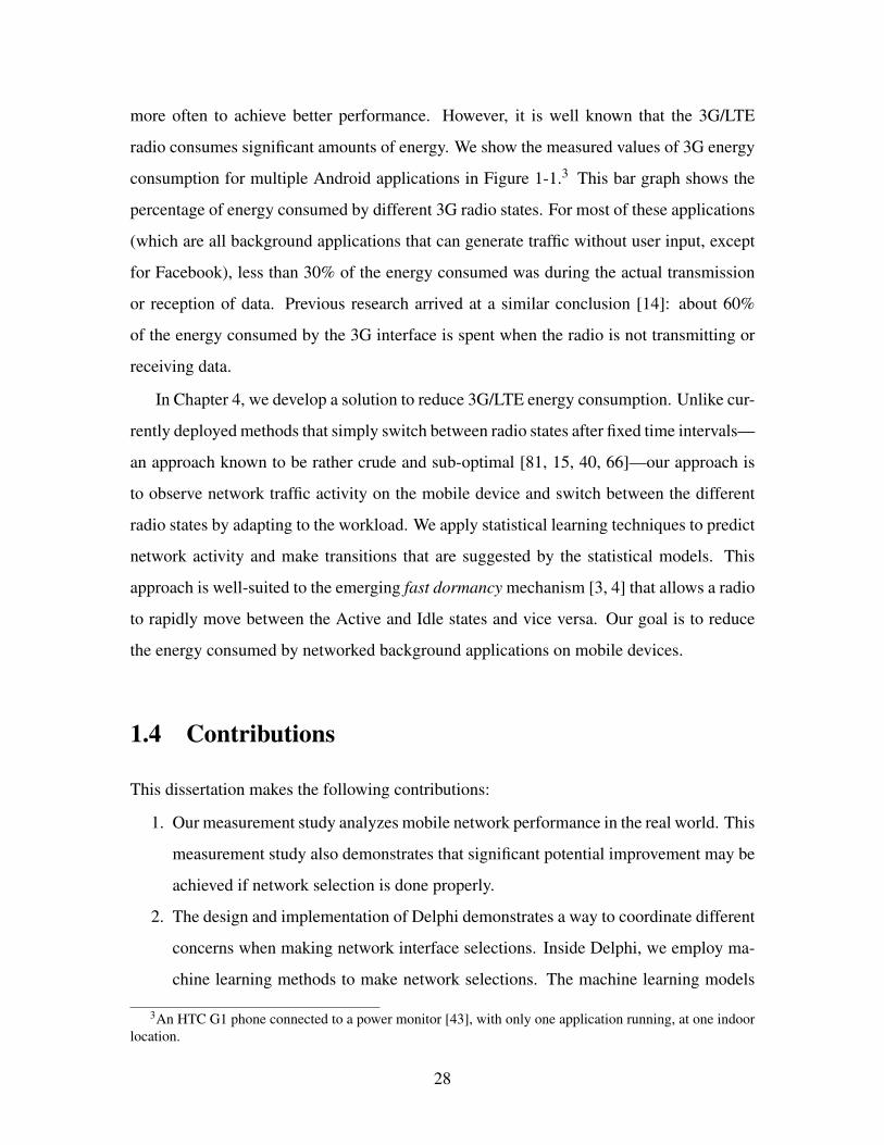
more often to achieve better performance. However, it is well known that the 3G/LTE
radio consumes significant amounts of energy. We show the measured values of 3G energy
consumption for multiple Android applications in Figure 1-1.3 This bar graph shows the
percentage of energy consumed by different 3G radio states. For most of these applications
(which are all background applications that can generate traffic without user input, except
for Facebook), less than 30% of the energy consumed was during the actual transmission
or reception of data. Previous research arrived at a similar conclusion [14]: about 60%
of the energy consumed by the 3G interface is spent when the radio is not transmitting or
receiving data.
In Chapter 4, we develop a solution to reduce 3G/LTE energy consumption. Unlike cur-
rently deployed methods that simply switch between radio states after fixed time intervals—
an approach known to be rather crude and sub-optimal [81, 15, 40, 66]—our approach is
to observe network traffic activity on the mobile device and switch between the different
radio states by adapting to the workload. We apply statistical learning techniques to predict
network activity and make transitions that are suggested by the statistical models. This
approach is well-suited to the emerging fast dormancy mechanism [3, 4] that allows a radio
to rapidly move between the Active and Idle states and vice versa. Our goal is to reduce
the energy consumed by networked background applications on mobile devices.
1.4 Contributions
This dissertation makes the following contributions:
1. Our measurement study analyzes mobile network performance in the real world. This
measurement study also demonstrates that significant potential improvement may be
achieved if network selection is done properly.
2. The design and implementation of Delphi demonstrates a way to coordinate different
concerns when making network interface selections. Inside Delphi, we employ ma-
chine learning methods to make network selections. The machine learning models
3An HTC G1 phone connected to a power monitor [43], with only one application running, at one indoorlocation.
28

are trained using network performance data we collected during the measurement
study. In the future, as wireless networks advance, the specific parameters we trained
for the current solution or even the machine learning algorithm may not be applica-
ble to make good network selections; however, our modular design makes sure that
the algorithms can be easily replaced. Thus, as long as there are co-existing net-
works whose performances are not evenly distributed spatially or temporally, Del-
phi’s framework can always be applicable.
3. Both our network selection and energy-efficient solutions require no modification to
the application running on the mobile devices. Thus, they can be easily deployed and
improve the performance and user experience of millions of apps already deployed.
1.5 Outline
The rest of this dissertation is organized as follows. Chapter 2 describes our measurement
study on the performance of Wi-Fi and cellular networks as well as transferring data on
both networks. Chapter 3 presents the design, implementation and evaluation for Delphi.
Chapter 4 analyzes the energy-efficiency issue of cellular networks in detail and presents
our solution to reduce energy consumption. Chapter 5 concludes the dissertation and dis-
cusses directions for future work.
29

30
Chapter 2
Measurement Study
Access to Wi-Fi and cellular wireless networks is de rigueur on mobile devices today.
With the emergence of LTE, cellular performance is starting to rival the performance of
Wi-Fi. Moreover, when Wi-Fi signal quality is low or in crowded settings, the anecdotal
experience of many users is that cellular performance may in fact be considerably better
than Wi-Fi performance. But just how good are LTE and Wi-Fi networks in practice, and
how do they compare with each other? Should applications and transport protocols strive to
select the best network, or should they simply always use Multi-Path TCP (MPTCP) [77]?
To answer these questions, we implemented a crowd-sourced network measurement
tool (§ 2.1) to understand the flow-level performance of TCP over Wi-Fi and LTE in the
wild from 16 different countries over a nine-month period, encompassing 3,632 distinct
1-Mbyte TCP flows. We used this data to measure transfer times for different amounts of
data transferred.
MPTCP is not widely deployed yet on most phones.1 As a result, we manually mea-
sured flow-level MPTCP performance and compared it with the performance of TCP run-
ning exclusively over Wi-Fi or LTE in 20 different locations, in 7 cities in the United
States (§ 2.2). Finally, to complement our empirical flow-level analysis, we used an ex-
isting record-and-replay tool to analyze (§ 2.3) and run (§ 2.4) mobile apps on emulated
cellular and Wi-Fi links, using it to study the impact of network selection on application
1The Apple iOS is an exception [49]. MPTCP is observed to be used for Siri. MPTCP on iOS operatesin master-backup mode using Wi-Fi as the primary path, falling back to a cellular path only if Wi-Fi isunavailable.
31

Figure 2-1: Cell vs. Wi-Fi User Interface.
performance.
2.1 Cell vs. Wi-Fi Measurement
In September 2013, we published an Android app on Google Play, called Cell vs. Wi-Fi
(http://web.mit.edu/cell-vs-wifi). Cell vs. Wi-Fi measures end-to-end Wi-
Fi and cellular network performance and uses these measurements to tell smartphone users
if they should be using the cellular network or Wi-Fi at the current time and location. The
app also serves as a crowd-sourced measurement tool by uploading detailed measurement
data to our server, including packet-level traces. Over a nine-month period after the app
was published, it attracted over 750 downloads. We collected over 10 GB of measurement
data from 3,632 distinct TCP connections over this duration from these users.
2.1.1 Cell vs. Wi-Fi App
Figure 2-1 shows the user interface of Cell vs. Wi-Fi. Users can choose to measure network
performance periodically or once per click. Users can also set an upper bound on the
32

① Start Measurement
Wi-Fi on? No
Turn Wi-Fi on
Wi-Fi Associated?
No Scan and Associate
Success?
Yes
② Measure Wi-Fi
Yes Yes
Turn Wi-Fi off
Cellular Available?
No
③ Measure Cellular Networks
Yes
Wi-Fi Available?
Turn Wi-Fi on
Yes
No
④ Upload Data
No
Figure 2-2: Cell vs. Wi-Fi: single measurement collection run.
amount of cellular data that the app can consume, especially for devices on a limited cellular
data plan.
33

The flow chart in Figure 2-2 shows a single measurement collection run. When the user
clicks the Start button, or the pre-set periodic measurement timer expires, one run of
measurement collection starts, shown as Step 1 in the figure. If Wi-Fi is available, and the
phone successfully associates with an Access Point (AP), Cell vs. Wi-Fi collects packet-
level tcpdump traces for a 1-Mbyte TCP upload and a 1-Mbyte TCP download between
the mobile device and our server at MIT.
After measuring Wi-Fi, Cell vs. Wi-Fi turns off the Wi-Fi interface on the phone and
attempts to connect to the cellular network. If the user has turned off the cellular data
network, Cell vs. Wi-Fi aborts the cellular measurement. If Cell vs. Wi-Fi successfully
connects to the cellular network, then in Step 3 it collects a similar set of packet-level
tcpdump traces for both an upload and a download. Once both Wi-Fi and cellular network
measurements are finished, in Step 4 Cell vs. Wi-Fi uploads the data collected during this
measurement run, together with the user ID (randomly generated when a smartphone user
uses the app for the first time) and the phone’s geographic location, to our server at MIT.
More information about Cell vs. Wi-Fi can be found at http://web.mit.edu/
cell-vs-wifi.
2.1.2 Results
Cell vs. Wi-Fi collected network-performance data from locations in five continents: North
America, South America, Europe, Africa, and Asia. We observed that some users use this
app to measure only Wi-Fi or LTE performance, but not both. We do not consider these
measurement runs because our goal is to compare LTE and Wi-Fi performance at nearly the
same place and time. To ensure that we measured only performance of LTE or an equivalent
high-speed cellular network, such as HSPA+, we used the Android network-type API [12]
and picked only those measurement runs that used LTE or HSPA+. When using the term
LTE in this dissertation, we mean either LTE or HSPA+. After these filtering steps, our
dataset contains over 1,606 complete runs of measurement, that is, both LTE and Wi-Fi
transfers in both directions.
In Table 2.1, we group nearby runs together using a k-means clustering algorithm, with
34

Location Name (Lat, Long) # of Runs LTE %US (Boston, MA) (42.4, -71.1) 884 10%
Israel (31.8, 35.0) 276 55%US (Portland) (45.6, -122.7) 164 45%
Estonia (59.4, 27.4) 124 71%South Korea (37.5, 126.9) 108 66%US (Orlando) (28.4, -81.4) 92 35%US (Miami) (26.0, -80.2) 84 52%
Malaysia (4.24, 103.4) 76 68%Brazil (-23.6, -46.8) 56 4%
Germany (52.5, 13.3) 40 20%Spain (28.0, -16.7) 40 80%
Thailand (Phichit) (16.1, 100.2) 40 80%US (New York) (40.9, -73.8) 24 33%
Japan (36.4, 139.3) 16 25%Sweden (59.6, 18.6) 16 0%
Thailand (Chiang Mai) (18.8, 99.0) 16 75%US (Chicago) (42.0, -88.2) 16 25%
Hungary (47.4, 16.8) 8 0%Italy (44.2, 8.3) 8 0%
US (Salt Lake City) (40.8, -111.9) 8 0%Colombia (7.1, -70.7) 4 0%
US (Santa Fe) (35.9, -106.3) 4 0%
Table 2.1: Geographical coverage and diversity of the crowd-sourced data collected from16 countries using Cell vs. Wi-Fi, ordered by number of runs collected. The last columnshows the percentage of runs in which LTE’s throughput is higher than Wi-Fi’s throughput.
a cluster radius of r = 100 kilometers (i.e., all runs in each group are within 200 kilometers
of each other). For each location group, we also list the percentage of measurement runs
where LTE has higher throughput than Wi-Fi does.
Figure 2-3 shows the CDF of difference in throughput between Wi-Fi and LTE on the
uplink and the downlink. We can see that the throughput difference can be larger than 10
Mbit/s in either direction. The gray region shows 42% (uplink) and 35% (downlink) of
the data samples whose LTE throughput is higher than Wi-Fi throughput. If we combine
uplink and downlink together, 40% of the time LTE outperforms Wi-Fi. Figure 2-4 shows
the CDF of ping RTT difference between LTE and Wi-Fi. During our measurement, we
sent 10 pings and took the average RTT value. The shaded area shows that in 20% of
35

0
0.2
0.4
0.6
0.8
1.0
-15 -10 -5 0 5 10 15 20 25
CD
F
Tput(Wi-Fi) - Tput(LTE) (mbps)
(a) Uplink
0
0.2
0.4
0.6
0.8
1.0
-15 -10 -5 0 5 10 15 20 25
CD
F
Tput(Wi-Fi) - Tput(LTE) (mbps)
(b) Downlink
Figure 2-3: CDF of difference between Wi-Fi and LTE throughput. The gray region shows42% (uplink) and 35% (downlink) of the data samples whose LTE throughput is higherthan Wi-Fi throughput.
0
0.2
0.4
0.6
0.8
1
-400 -200 0 200 400
CD
F
RTT(Wi-Fi) - RTT(LTE) (ms)
Figure 2-4: CDF of the difference between average Ping RTT with Wi-Fi and LTE. Thegray region shows 20% of the data samples whose LTE RTT is lower than Wi-Fi RTT.
our measurement runs, LTE has a lower ping RTT than Wi-Fi does, although the cellular
network is commonly assumed to have higher delays.
The simple network selection policy used by mobile devices today forces applications
to use Wi-Fi whenever available. However, our measurement results indicate that a more
flexible network selection policy will improve the network performance of mobile applica-
tions.
36
2.2 MPTCP Measurements
When Wi-Fi and cellular networks offer comparable performance, or when each varies sig-
nificantly with time, it is natural to use both simultaneously. Several schemes transmitting
data on multiple network interfaces have been proposed in the past [84, 62, 54, 77]. Among
these, the most widespread is MPTCP [77]. MPTCP can be used in two modes [57]: Full-
MPTCP mode, which transmits data on all available network interfaces at any time, and
Backup mode, which transmits data on only one network interface at a time, falling back
to the other interface only if the first interface is down. Unless stated otherwise, all experi-
ments in this chapter used MPTCP in Full-MPTCP mode. For completeness, we compare
the two modes in § 2.2.6. We used a modified version of Cell vs. Wi-Fi to carry out MPTCP
measurements. We observed the following:
1. We found that MPTCP throughput for short flows depends significantly on the net-
work selected for the primary subflow2 in MPTCP; for example, changing the net-
work (LTE or Wi-Fi) for the primary subflow changes the average throughput of a 10
KByte flow by 60% in the median (Figure 2-12 in § 2.2.4).
2. For long flows, selecting the proper congestion control algorithm is also important.
For example, using different congestion control algorithms (coupled or decoupled)
changes the average throughput of a 1 MByte flow by 34% in the median (Figure 2-
17 in § 2.2.5).
3. MPTCP’s Backup mode is typically used for energy efficiency: keeping fewer in-
terfaces active reduces energy consumption overall. However, we found that for
MPTCP in Backup mode, if LTE is set to the backup interface, very little energy can
be saved for flows that last shorter than 15 seconds (§ 2.2.6).
2.2.1 MPTCP Overview
MPTCP initiates a connection in a manner similar to regular TCP: it picks one of the
available interfaces and establishes a TCP connection using a SYN-ACK exchange with
the server over that interface. Every TCP connection that belongs to a MPTCP connection
2We define subflows in § 2.2.1.
37

is called an MPTCP subflow. The first established subflow is called the primary subflow.
We used the Linux MPTCP implementation for our measurements [52] (Ubuntu Linux
13.10 with Kernel version 3.11.0, with the MPTCP Kernel implementation version v0.88).
In this implementation, MPTCP initiates the primary subflow on the interface used as the
default route on the machine. Once the primary subflow is established, if there are other
interfaces available, MPTCP creates an additional subflow using each new interface and
combines the new subflow with the existing subflows on the same MPTCP connection.3
For example, a mobile device can establish an MPTCP primary subflow through Wi-Fi to
the server and then add an LTE subflow to the server. To terminate the connection, each
subflow is terminated using four-way FIN-ACKs, similar to TCP. In § 2.2.4 we study the
effect of choosing different interfaces for the primary subflow on MPTCP performance.
There are two kinds of congestion-control algorithms used by MPTCP: decoupled and
coupled. In decoupled congestion control, each subflow increases and decreases its conges-
tion window independently, as if they were independent TCP flows [19]. In coupled con-
gestion control, each subflow in an MPTCP connection increases its congestion window
based on ACKs both from itself and from other subflows [77, 37] in the same MPTCP con-
nection. In § 2.2.5 we compare the coupled and decoupled algorithms and find that using
different congestion control algorithms has less impact on throughput compared with se-
lecting the correct interface for primary subflows for short flows. However, for long flows,
changing congestion control algorithms results in a substantial throughput difference.
2.2.2 Measurement Setup
Figure 2-5 shows the MPTCP measurement setup. The MPTCP client is a laptop running
Ubuntu 13.10 with MPTCP installed. We tethered two smartphones to the laptop, one in
“airplane” mode with Wi-Fi enabled, and the other with Wi-Fi disabled but connected to
LTE (either the Verizon or the Sprint LTE network). The MPTCP server is located at MIT,
with a single Ethernet interface, also running Ubuntu 13.10 with MPTCP installed.
We installed a modified version of Cell vs. Wi-Fi on both phones. The phone with Wi-Fi
3For simplicity, here we explain only how MPTCP works when the server is single-homed (like the serverin our experiments), and the client alone is multi-homed.
38

Figure 2-5: Setup of MPTCP measurement.
enabled measures only Wi-Fi performance (Step 2 in Figure 2-2). The phone connected
to LTE measures only cellular network performance (Step 3 in Figure 2-2).
The experimental setup also allows us to measure the energy consumption separately
for each interface, which we present in § 2.2.6.
Each measurement run comprises the following:
1. Single-path TCP upload and download using modified Cell vs. Wi-Fi through LTE.
2. Single-path TCP upload and download using modified Cell vs. Wi-Fi through Wi-Fi.
3. MPTCP upload and download in Full-MPTCP mode with LTE as the primary sub-
flow.
4. MPTCP upload and download in Full-MPTCP mode with Wi-Fi as the primary sub-
flow.
We conducted the measurements at 20 different locations on the east and west coasts
of the United States, shown in Table 2.2. At each city, we conducted our measurement
at places where people would often use mobile devices: cafes, shopping malls, university
campuses, hotel lobbies, airports, and apartments. At 7 of the 20 locations, we measured
both Verizon and Sprint LTE networks using both MPTCP congestion-control algorithms:
decoupled and coupled. At the other 13 locations, we were able to measure only the Verizon
LTE network with coupled congestion control.
In Figure 2-6, we compare the Wi-Fi and LTE throughput distributions for the data we
39

ID City Description1 Amherst, MA University Campus, Indoor2 Amherst, MA University Campus, Outdoor3 Amherst, MA Cafe, Indoor4 Amherst, MA Downtown, Outdoor5 Amherst, MA Apartment, Indoor6 Boston, MA Cafe, Indoor7 Boston, MA Shopping Mall, Indoor8 Boston, MA Subway, Outdoor9 Boston, MA Airport, Indoor
10 Boston, MA Apartment, Indoor11 Boston, MA Cafe, Indoor12 Boston, MA Downtown, Outdoor13 Boston, MA Store, Indoor14 Santa Babara, CA Hotel Lobby, Indoor15 Santa Babara, CA Hotel Room, Indoor16 Santa Babara, CA Conference Room, Indoor17 Los Angeles, CA Airport, Indoor18 Washington, D.C. Hotel Room, Indoor19 Princeton, NJ Hotel Room, Indoor20 Philadelphia, PA Hotel Room, Indoor
Table 2.2: Locations where MPTCP measurements were conducted.
0
0.2
0.4
0.6
0.8
1.0
-15 -10 -5 0 5 10 15 20 25
CD
F
Tput(Wi-Fi) - Tput(LTE) (mbps)
App Data20-Location
(a) Uplink
0
0.2
0.4
0.6
0.8
1.0
-15 -10 -5 0 5 10 15 20 25
CD
F
Tput(Wi-Fi) - Tput(LTE) (mbps)
App Data20-Location
(b) Downlink
Figure 2-6: CDF for Wi-Fi and LTE throughput measured using regular TCP at 20 locations(shown as “20-Location”) compared with the CDF in Figure 2-3 (shown as “App Data”).
collected at these 20 locations and the data collected from Cell vs. Wi-Fi in § 2.1. We can
see that for both upload and download, the “20-Location” CDF curves are close to the CDF
40

curves from § 2.1, implying that the 20 locations that were selected have similar variability
in network conditions as the Cell vs. Wi-Fi dataset. For simplicity, in the rest of § 2.2, we
show only results of downlink flows from the server to the client.
2.2.3 TCP vs. MPTCP
0
1
2
3
4
5
6
7
8
9
10
1 10 100 1000
Th
rou
gh
pu
t (m
bp
s)
Flow Size (KB)
LTEWi-Fi
MPTCP(LTE, Decoupled)MPTCP(Wi-Fi, Decoupled)
MPTCP(LTE, Coupled)MPTCP(Wi-Fi, Coupled)
(a) MPTCP performs worse than single TCP.
0
1
2
3
4
5
6
7
8
9
10
1 10 100 1000
Th
rou
gh
pu
t (m
bp
s)
Flow Size (KB)
LTEWi-Fi
MPTCP(LTE, Decoupled)MPTCP(Wi-Fi, Decoupled)
MPTCP(LTE, Coupled)MPTCP(Wi-Fi, Coupled)
(b) MPTCP performs better than single TCP.
Figure 2-7: MPTCP throughput vs single-path TCP throughput at 2 representative loca-tions. Figure 2-7a shows a case in which MPTCP throughput is lower than the best through-put of single-path TCP. Figure 2-7b shows a case where MPTCP throughput (in this case,MPTCP (Wi-Fi, decoupled)) is higher than that of single-path TCP for large flow sizes.
A natural question pertaining to MPTCP is how the performance of MPTCP compares
with the best single-path TCP performance achievable by an appropriate choice of networks
alone. To answer this, we looked at all four MPTCP variants (two congestion control
algorithms times two choices for the network used by the primary subflow) and both single-
path TCP variants (Wi-Fi and LTE) as a function of flow size. Figure 2-7 illustrates two
qualitatively different behaviors.
Figure 2-7a shows a case in which the performance of MPTCP is always worse than
the best single-path TCP regardless of flow size. This occurs in a particularly extreme
scenario in which a large disparity in link speeds between the two networks (LTE and Wi-
Fi) leads to degraded MPTCP performance irrespective of flow size. On the other hand,
Figure 2-7b shows an alternative scenario where MPTCP is better than the best single-path
TCP at larger flow sizes. In both cases, however, picking the right network for single-path
41

0
500
1000
1500
2000
2500
3000
0 1 2 3 4 5
Acke
d S
eq
Nu
mb
er
(KB
yte
s)
Time (sec)
TCP MPTCP
Figure 2-8: Acknowledged data vs. time for TCP and MPTCP.
400
450
500
550
600
650
700
750
800
0.8 0.9 1 1.1 1.2 1.3 1.4 1.5
Se
q N
um
be
r (K
Byte
s)
Time (sec)
Wi-Fi SeqWi-Fi AckLTE SeqLTE Ack
(a) Sender Side
400
450
500
550
600
650
700
0.8 0.9 1 1.1 1.2 1.3 1.4 1.5
Se
q N
um
be
r (K
Byte
s)
Time (sec)
Wi-Fi SeqWi-Fi AckLTE SeqLTE Ack
(b) Receiver Side
Figure 2-9: MPTCP sent and acknowledged data sequence number vs. time on sender andreceiver side.
TCP is preferable to using MPTCP for smaller flows. These results suggest that it may not
always be advisable to use both networks, and an adaptive policy that automatically picks
the networks to transmit on and the transport protocol to use would improve performance
relative to any static policy.
To investigate why MPTCP do not give higher throughput in certain cases, we con-
42

ducted experiments in a lab environment where Wi-Fi has a much higher link speed than
LTE has. Figure 2-8 shows the ACK packet seen on the sender side when using Wi-Fi for
single-path TCP and using Wi-Fi and LTE for MPTCP. We can see that between time 1.0
second and 1.5 seconds, the MPTCP sender sees fewer ACKs; thus, the average throughput
decreases. To explain why MPTCP slows down at time 1.0 second, Figure 2-9 shows the
MPTCP data sequence numbers sent out and ACK sequence numbers received on its Wi-Fi
subflow and LTE subflow. We can see that in Figure 2-9a MPTCP starts sending data on
the LTE subflow at time 0.82 seconds. It sends out 10 back-to-back packets (with sequence
numbers from 514008 bytes to 519720 bytes) because the initial congestion control win-
dow is set to 10 by default. The LTE subflow receives the first ACK at time 1.02 seconds,
that is, the RTT for LTE subflow is 0.2 seconds, much longer than Wi-Fi subflow’s RTT
(which is 0.03 seconds on average during this transfer). However, as shown in Figure 2-9b,
due to long delays on the LTE subflow, it receives the first three data packets on the LTE
subflow at 1.0, 1.02, and 1.16 seconds, respectively. Since MPTCP sends ACKs with the
highest in-order received sequence number, it keeps sending ACKs with sequence number
515436 to the sender although the Wi-Fi subflow has sent out packets with higher sequence
numbers. This causes the Wi-Fi subflow to stop sending higher sequence number packets
and to start retransmitting packets with sequence number 515436 at time 1.18 seconds. The
retransmission phase ends at time 1.45 seconds because there are 10 packets scheduled to
be sent on the LTE subflow at the beginning, and the sender needs to make sure all 10
packets are received before it can transmit further packets. In this case, seven packets are
retransmitted on the Wi-Fi subflow. This effect is mentioned as “head-of-line blocking” in
previous work [58].
One possible approach to reduce throughput degradation caused by head-of-line block-
ing is to reduce the initial congestion control window; thus, the Wi-Fi subflow will retrans-
mit fewer packets. To verify this assumption, we configured the initial congestion control
window for MPTCP to be 1 and ran the same experiment. The results are shown in Fig-
ures 2-10 and 2-11. We can see that in Figure 2-11a because only one packet is sent on
the LTE subflow at time 0.31 seconds, and is ACKed at time 0.47 seconds, there is no more
retransmission on the Wi-Fi path due to head-of-line blocking.
43

0
500
1000
1500
2000
2500
3000
0 1 2 3 4 5
Acke
d S
eq
Nu
mb
er
(KB
yte
s)
Time (sec)
TCP MPTCP
Figure 2-10: Acknowledged data vs. time for TCP and MPTCP when initial congestioncontrol window is 1 MSS.
0
50
100
150
200
250
300
350
400
0 0.1 0.2 0.3 0.4 0.5 0.6
Se
q N
um
be
r (K
Byte
s)
Time (sec)
Wi-Fi SeqWi-Fi AckLTE SeqLTE Ack
(a) Sender Side
0
50
100
150
200
250
300
0 0.1 0.2 0.3 0.4 0.5 0.6
Se
q N
um
be
r (K
Byte
s)
Time (sec)
Wi-Fi SeqWi-Fi AckLTE SeqLTE Ack
(b) Receiver Side
Figure 2-11: MPTCP sent and acknowledged data sequence number vs. time on sender andreceiver side, when initial congestion control window is 1 MSS.
2.2.4 Primary Flow Measurement
We then studied how the choice of the network for the primary subflow can affect MPTCP
throughput for different flow sizes. To show this quantitatively, we calculate the relative
throughput difference as:
44

0
0.1
0.2
0.3
0.4
0.5
0.6
0.7
0.8
0.9
1
0 50 100 150 200
CD
F
Relative Difference(%)
10 KB100 KB
1 MB
Figure 2-12: CDF of relative difference between MPTCPLT E and MPTCPWi−Fi, for differ-ent flow sizes. The median relative difference for each flow size is: 60% for 10 KBytes,49% for 100 KBytes and 28% for 1MByte. Thus, throughput for smaller flow sizes is moreaffected by the choice of the network for the primary subflow.
|MPTCPLT E−MPTCPWi−Fi|MPTCPWi−Fi
.
Here, MPTCPLT E is the throughput achieved by MPTCP using LTE for the primary
subflow, and MPTCPWi−Fi is the throughput achieved by MPTCP using Wi-Fi for the pri-
mary subflow (in this subsection, we ran MPTCP using only decoupled congestion control).
Figure 2-12 shows the CDF of the relative throughput difference for three flow sizes: 10
KBytes, 100 KBytes, and 1 MByte. We see that using different networks for the primary
subflow has the greatest effect on smaller flow sizes.
2.2.4.1 MPTCP Throughput Evolution Over Time
To understand how using different networks for the primary subflow affects MPTCP through-
put evolution over time, we collected tcpdump traces at the MPTCP client during the
measurement. From the traces, we calculated the average throughput from the time the
MPTCP session was established, to the current time t. In Figures 2-13 and 2-14, we plot
45

0
0.5
1
1.5
2
2.5
3
0 0.5 1 1.5 2
Tp
ut
(mb
ps)
Time (second)
LTEWi-Fi
MPTCP
(a) Using Wi-Fi for the primary subflow
0
1
2
3
4
5
6
7
0 0.5 1 1.5 2
Tp
ut
(mb
ps)
Time (second)
LTEWi-Fi
MPTCP
(b) Using LTE for the primary subflow
Figure 2-13: MPTCP throughput over time, measured at a location where LTE had higherthroughput than Wi-Fi had. MPTCP throughput grows faster over time when using LTEfor the primary subflow.
0
1
2
3
4
5
6
0 0.5 1 1.5 2
Tp
ut
(mb
ps)
Time (second)
LTEWi-Fi
MPTCP
(a) Using Wi-Fi for the primary subflow
0
0.5
1
1.5
2
2.5
3
3.5
4
4.5
0 0.5 1 1.5 2
Tp
ut
(mb
ps)
Time (second)
LTEWi-Fi
MPTCP
(b) Using LTE for the primary subflow
Figure 2-14: MPTCP throughput over time, measured at a location where Wi-Fi had higherthroughput than LTE had. MPTCP throughput grows faster over time when using Wi-Fifor the primary subflow.
the average throughput as a function of time. Each sub-figure shows the throughput of the
entire MPTCP session (shown as MPTCP) and the throughput of the individual Wi-Fi and
LTE subflows.
Figure 2-13 shows traces collected at a location where LTE had much higher throughput
than Wi-Fi had. At time 0, the client sent the SYN packet to the server. In Figure 2-13a,
it took the client 1 second to receive the SYN-ACK packet from the server over Wi-Fi.
MPTCP throughput was the same as the throughput of the Wi-Fi subflow until the LTE
46

subflow was established. Because LTE had much higher throughput at this location and
time, once the subflow was established on LTE, it quickly increased its throughput (and
therefore MPTCP’s throughput). By contrast, in Figure 2-13b, the client received the SYN-
ACK faster, and MPTCP throughput increased more quickly because the first subflow was
on the higher-throughput LTE network. Because of the smaller SYN-ACK RTT and higher
throughput on the first primary subflow, the MPTCP connection using LTE for the primary
subflow (Figure 2-13b) had a higher average throughput than the MPTCP connection using
Wi-Fi for the primary subflow (Figure 2-13a).
Similarly, Figure 2-14 shows traces collected at a location where Wi-Fi had higher
throughput than LTE had. Here, using Wi-Fi as the primary subflow for MPTCP results in
higher throughput.
2.2.4.2 MPTCP Throughput as a Function of Flow Size
0
1
2
3
4
5
6
0 200 400 600 800 1000
Th
rou
gh
pu
t (m
bp
s)
Flow size (KB)
MPTCP(LTE)MPTCP(Wi-Fi)
(a) Absolute throughput difference: larger dif-ference between Wi-Fi and LTE for larger flowsizes.
0
0.5
1
1.5
2
2.5
3
0 200 400 600 800 1000
Th
rou
gh
pu
t R
atio
Flow size (KB)
MPTCP(LTE)MPTCP(Wi-Fi)
(b) Relative throughput ratio: larger differencebetween Wi-Fi and LTE for smaller flow sizes.
Figure 2-15: Absolute throughput difference and relative throughput ratio as a function offlow size when LTE has higher throughput than Wi-Fi has.
Figures 2-15a and 2-16a show how MPTCP throughput changes as the flow size in-
creases. The flow size is measured using the cumulative number of bytes acknowledged in
each ACK packet received at the MPTCP client. Figures 2-15b and 2-16b show the relative
throughput ratio change as flow size increases. The relative throughput ratio is defined as:
47
0
0.5
1
1.5
2
2.5
3
3.5
4
4.5
5
0 200 400 600 800 1000
Th
rou
gh
pu
t (m
bp
s)
Flow size (KB)
MPTCP(LTE)MPTCP(Wi-Fi)
(a) Absolute throughput difference: larger dif-ference between Wi-Fi and LTE for larger flowsizes.
0
0.5
1
1.5
2
0 200 400 600 800 1000
Th
rou
gh
pu
t R
atio
Flow size (KB)
MPTCP(LTE)MPTCP(Wi-Fi)
(b) Relative throughput ratio: larger differencebetween Wi-Fi and LTE for smaller flow sizes.
Figure 2-16: Absolute throughput difference and relative throughput ratio as a function offlow size when Wi-Fi has higher throughput than LTE has.
MPTCPLT EMPTCPWi−Fi
.
Although the absolute value of the difference in throughputs is smaller for small flow
sizes (Figures 2-15a and 2-16a), the relative throughput ratio is larger (Figures 2-15b and 2-
16b). Thus, for a connection with a given flow size, using the correct interface for MPTCP
primary subflow can reduce the flow completion time, and the relative reduction can be
significant for smaller flow sizes. For example, in Figure 2-15a, the absolute throughput
difference between LTE and Wi-Fi is 0.5 Mbit/s for a 100-KByte flow, and about 3 Mbit/s
for a 1-MByte flow. But in Figure 2-15b, the relative throughput ratio is 2.2× for a 100-
KBybte flow, larger than the 1.5× for a 1-MByte flow.
2.2.5 Coupled and Decoupled Congestion Control
To understand how the choice of congestion control algorithm within MPTCP affects its
throughput, at 7 of the 20 locations, we measured the following different MPTCP configu-
rations on the Verizon LTE network and each location’s dominant Wi-Fi network:
1. LTE for primary subflow, coupled congestion control.
2. LTE for primary subflow, decoupled4 congestion control.
4Here, the decoupled congestion control uses TCP Reno for each subflow.
48

3. Wi-Fi for primary subflow, coupled congestion control.
4. Wi-Fi for primary subflow, decoupled congestion control.
At each location, we measured 10 runs for each of the 4 configurations, along both
the uplink and the downlink. Thus, each of the four configurations has 140 data points
((10+10)×7).
0
0.1
0.2
0.3
0.4
0.5
0.6
0.7
0.8
0.9
1
0 50 100 150 200
CD
F
Relative Difference(%)
10 KB100 KB
1 MB
Figure 2-17: CDF of relative difference between MPTCPcoupled and MPTCPdecoupled , fordifferent flow sizes. The median relative difference for each flow size: 16% for 10 KBytes,16% for 100 KBytes and 34% for 1 MByte. Thus, throughput for larger flow sizes is mostaffected by the choice of congestion control.
To quantify the throughput difference between configurations, we compute:
rnetwork =|MPTCPLT E,coupled−MPTCPWi−Fi,coupled |
MPTCPWi−Fi,coupled, or
rnetwork =|MPTCPLT E,decoupled−MPTCPWi−Fi,decoupled |
MPTCPWi−Fi,decoupled.
Here, rnetwork is the relative throughput difference when using different networks for
primary subflow. MPTCPn,c is the throughput measured when using network n for primary
subflow and using congestion control algorithm c. We also compute:
rcwnd =|MPTCPLT E,decoupled−MPTCPLT E,coupled |
MPTCPLT E,coupled, or
49

rcwnd =|MPTCPWi−Fi,decoupled−MPTCPWi−Fi,coupled |
MPTCPWi−Fi,coupled.
Here, rcwnd is the relative throughput difference when using different congestion control
algorithms.
0
0.1
0.2
0.3
0.4
0.5
0.6
0.7
0.8
0.9
1
0 50 100 150 200
CD
F
Relative Difference(%)
CCNetwork
(a) 10 KB
0
0.1
0.2
0.3
0.4
0.5
0.6
0.7
0.8
0.9
1
0 50 100 150 200
CD
F
Relative Difference(%)
CCNetwork
(b) 100 KB
0
0.1
0.2
0.3
0.4
0.5
0.6
0.7
0.8
0.9
1
0 50 100 150 200
CD
F
Relative Difference(%)
CCNetwork
(c) 1 MB
Figure 2-18: CDF of relative difference using different networks for primary subflow (la-beled as “Network”) vs. using different congestion control algorithms (labeled as “CC”),across 3 flow sizes. Median values for CC curves are: 16% for “10 KB”, 16% for “100KB”, and 34% for “1 MB”. Thus, using different congestion control algorithms has moreimpact on larger flows. Median values for Network curves are: 60% for “ 10 KB”, 43% for“100 KB” , and 25% for “1 MB”. Thus, using a different network for the primary subflowhas greater impact on smaller flows.
Figure 2-17 shows the CDF of the relative throughput difference between using coupled
and decoupled congestion control for three flow sizes: 10 KBytes, 100 KBytes, and 1
MByte. The rightmost CDF curve corresponds to the relative difference for 1 MByte, while
the left-most one is for 10 KBytes. Thus, using different congestion control algorithms has
a greater impact on larger flow sizes. In Figure 2-18, a pair-wise comparison between
using different networks (labeled with“Network”) and using different congestion control
algorithms (labeled with “CC”) for each flow size shows the following:
1. For small flow sizes, throughput is more affected by the choice of network for the
primary subflow. For example, in Figures 2-18a and 2-18b, “Network” is to the right
of “CC”.
2. For large flow sizes, throughput is more affected by the choice of congestion control
(decoupled or coupled) algorithms. For example: in Figure 2-18c, “CC” is to the
right of “Network”. However, the choice of network for the primary subflow is also
important.
50

In practice, selecting the best network for the primary subflow is more feasible than
changing congestion control algorithms for each MPTCP connection, since the primary
flow can be defined solely by the MPTCP endpoint initiating the connection, while the
congestion control algorithm requires support at both endpoints.
2.2.6 Full-MPTCP and Backup Modes
In § 2.2.4 and § 2.2.5, all measurements were done using Full-MPTCP mode, since our
focus was on how MPTCP’s throughput changes under different configurations, when all
paths are fully utilized. Backup mode is an MPTCP mode where only a subset of paths are
used to save energy, especially on power-constrained mobile devices. In this section, we
first show how Backup mode differs from Full-MPTCP at the per-packet level. Then we
discuss the energy efficiency of both Full-MPTCP and Backup modes.
2.2.6.1 Packet-Level Behavior of Full-MPTCP and Backup Modes
Figure 2-19 shows the packet-transmission pattern over time for a long flow employing
MPTCP, using Full-MPTCP and Backup modes. We use tcpdump at the MPTCP client to
log packet transmission and ACK reception times. In Figure 2-19, we plot a vertical line at
time t if there is a packet sent or ACK received at time t in the tcpdump trace. t = 0 is the
time when the first SYN packet is sent. Each sub-figure contains the packet-transmission
patterns on both the Wi-Fi and LTE interfaces for one MPTCP flow. Sub-figures on the left
column are packet transmission (sending and receiving) patterns captured when using LTE
for the primary subflow, while sub-figures on the right are for using Wi-Fi for the primary
subflow.
Figures 2-20a and 2-20b show that in Full-MPTCP mode, packets are transferred through
both Wi-Fi and LTE during the entire MPTCP connection.
Figures 2-19c and 2-19d illustrate the Backup mode where one network is set to be
the backup interface. For example, in Figure 2-19c, when Wi-Fi is set to backup, we see
only the SYN and SYN ACK packets transferred during the 3-way handshake procedure
at t = 1, when the connection establishes a Wi-Fi subflow, as well as FIN and FIN-ACK
51

LTE
0 5 10 15 20
Time (sec)
Wi-Fi
(a) Full-MPTCP, using LTE forprimary subflow.
LTE
0 5 10 15 20
Time (sec)
Wi-Fi
(b) Full-MPTCP, using Wi-Fi forprimary subflow.
LTE
0 5 10 15 20
Time (sec)
Wi-Fi
(c) Backup mode, using LTEfor primary subflow, Wi-Fi forbackup.
LTE
0 10 20 30 40 50
Time (sec)
Wi-Fi
(d) Backup mode, using Wi-Fi forprimary subflow, LTE for backup.
LTE
0 5 10 15 20 25 30 35 40 45
Time (sec)
Wi-Fi
(e) Backup mode, using LTEfor primary subflow, Wi-Fi forbackup. Then, set LTE to “multi-path off” at t = 9 sec.
LTE
0 5 10 15 20 25 30 35
Time (sec)
Wi-Fi
(f) Backup mode, using Wi-Fi forprimary subflow, LTE for backup.Then, set Wi-Fi to “multipath off”at t = 11 sec.
LTE
0 10 20 30 40 50 60 70 80 90
Time (sec)
Wi-Fi
(g) Backup mode, using LTEfor primary subflow, Wi-Fi forbackup. Unplug LTE at t = 3 sec,but Wi-Fi does not continue trans-ferring the rest of the data. PlugLTE back in at t = 68 sec.
LTE
0 5 10 15 20
Time (sec)
Wi-Fi
(h) Backup mode, using Wi-Fi forprimary subflow, LTE for backup.Unplug Wi-Fi at t = 6 sec.
Figure 2-19: Full-MPTCP and Backup modes.52

packets at t = 19, when the connection ends. A similar pattern is shown in Figure 2-19d,
when LTE is set to be the backup interface.
Figures 2-19e and 2-19f show packet transmissions in Backup mode when the primary
network is disabled mid-flow. We disable the interface by setting the interface to “multipath
off” in iproute. In Figure 2-19e, Wi-Fi is set to backup. When the connection starts,
it transfers data through LTE. At t = 7, we disable LTE so no data can be transferred over
that interface. We see that the subflow over Wi-Fi is brought up and transfers data until the
flow ends. A similar behavior is seen in Figure 2-19f.
In Figures 2-19g and 2-19h, we disable one network by unplugging the USB cable
connecting the phone to the laptop instead of disabling it using iproute. Interestingly,
we observe different behaviors in this experiment. Figure 2-19h shows that when LTE is
set to backup, and we unplug Wi-Fi in the middle of the transfer (at t = 6), the LTE path is
brought up immediately to finish transferring the rest of the data. This behavior is similar to
when Wi-Fi was disabled by changing iproute. However, in Figure 2-19g, when Wi-Fi
is set to backup and we unplug the LTE network in the middle of the transfer (at t = 3), the
client transfers only one TCP Window Update packet to the server through the Wi-Fi
subflow and then halts. At t = 68, we re-connect the phone with the laptop. Then, the
connection resumes, transfers the rest of the data through the LTE subflow, and ends the
session by sending FIN packets on both path.
The reason disabling paths by physically disconnecting them can cause different be-
haviors from disabling them in software is still under investigation.
2.2.6.2 Energy Efficiency in Backup Mode
As shown in Figures 2-19c and 2-19d, if MPTCP is set to Backup mode, the backup inter-
face still transfers SYN and FIN packets when a connection starts and ends. In Figure 2-
20, we show that in certain configurations, these SYN/FIN packets can consume excessive
amounts of energy on a mobile device. Here, we measure the power level of the tethered
phones using a power monitor [43] when each phone serves as the backup or non-backup
interface. In all sub-figures of Figure 2-20, the base power consumed is 1 watt. This is the
power consumed when the network interfaces are not active. It is the total power consumed
53

Time (Sec)0 10 20 30 40 50
Power (w
)
4
3
2
1
0
FINSYN
(a) LTE power level when used for non-backup subflow.
Time (Sec)0 10 20 30 40 50
Power (w
)
4
3
2
1
0
FINSYN
(b) Wi-Fi power level when used for non-backup subflow.
Time (Sec)0 10 20 30 40 50
Power (w
)
4
3
2
1
0
FINSYN
(c) LTE power level when used for backupsubflow.
Time (Sec)0 10 20 30 40 50
Power (w
)
4
3
2
1
0
FINSYN
(d) Wi-Fi power level when used for backupsubflow.
Figure 2-20: Power level for LTE and Wi-Fi when used as non-backup subflow. LTE has amuch higher power level than Wi-Fi in non-backup mode. LTE also consumes an excessiveamount of energy even in backup mode.
by the other parts of the phone, such as the screen and the CPU.
Figure 2-20a shows the power level of LTE when it is actively transmitting data, that is,
Wi-Fi is set as a backup interface. Similarly, Figure 2-20b shows the power level of Wi-Fi
when it is active. We can see that the Wi-Fi power level is much lower than that of LTE.
Also, in Figure 2-20a, after the FIN packet is sent, there is a 15-second period in which
the LTE power level stays at 2 watts, instead of the 1-watt base power level. The energy
consumed in this 15-second period is called the tail energy [16, 26].
Figures 2-20c and 2-20d show the power level when Wi-Fi or LTE is set to be the
backup interface. In Figure 2-20d, the energy consumed by Wi-Fi is negligible. However,
in Figure 2-20c, when a SYN or a FIN packet is transmitted through LTE, the power level
stays high for about 15 seconds due to the tail energy effect. Thus, even if only SYN and
FIN packets are transferred through LTE, the LTE interface still consumes an excessive
amount of energy. For flows shorter than 15 seconds, little energy can be saved if the
LTE interface is set to be the backup interface. To actually reduce energy consumption in
54

this case, fast dormancy [31] should be used to quickly put the LTE interface in the low-
power mode after a SYN and FIN. Alternatively, the Backup mode should be implemented
in a break-before-make manner. Prior work [57] has proposed Single-Path mode, which
establishes a new MPTCP subflow only after the current subflow is inactive, at the expense
of two more round-trip times compared with the current Backup mode.
2.3 Mobile App Traffic Patterns
So far, our measurements have looked at the flow-level performance of TCP over Wi-Fi or
LTE, and of MPTCP over both Wi-Fi and LTE. We next turn to how the choice of networks
for a multi-homed mobile device affects application-level performance as perceived by a
mobile app that uses one or more of these networks. To measure performance at the level of
a mobile app, we first record (§2.3.1) and analyze traffic (§2.3.2) originating from a mobile
app, and then replay it under emulated link conditions (§2.4).
2.3.1 Record-Replay Tool
Mahimahi [53] is a record-and-replay tool that can record and replay client-server interac-
tions over HTTP. Mahimahi’s RecordShell is a UNIX shell that records HTTP traffic and
stores it as a set of request-response pairs. Later, during replay, Mahimahi’s ReplayShell—
another modified UNIX shell—matches incoming requests to stored requests, ignoring
time-sensitive fields in the request header (e.g., If-Modified-Since) that have likely changed
since recording.
Mahimahi also includes shells to emulate network delays and fixed-rate and variable-
rate network links using packet-delivery traces. We extend these capabilities and develop a
new shell, MpShell, to emulate multiple links along with their associated link delays. This
allows us to mimic a multi-homed mobile phone that can use both cellular and Wi-Fi links.
We use a trace-driven approach, as Mahimahi does, to emulate both the cellular and Wi-Fi
links.
Because Mahimahi is agnostic to the specific client or server that generates the HTTP
traffic, we use it to record all HTTP traffic to and from a mobile app running inside an An-
55

droid emulator. Later, using ReplayShell and MpShell, we run the same mobile app within
the Android emulator under appropriately emulated network conditions. This enables us
to evaluate how MPTCP—or any other multipath-capable transport—affects application
performance of a real mobile app.
2.3.2 Traffic Patterns of Mobile Apps
Figure 2-21 shows typical traffic patterns we observed across different mobile apps run
inside RecordShell. We observed that apps tend to initiate multiple TCP connections when
launched or in response to a user interaction. Most of these connections transfer only a
small amount of data (e.g., connection ID 2 in Figure 2-21c). Some connections, such as
connection ID 2 in Figure 2-21a, persist after small data transfers.
A few connections, such as connection ID 30 in Figure 2-21d and connection ID 8
in Figure 2-21f, transfer significant amounts of data, lasting several seconds. The first
example (ID 30) occurred when the user clicked a link to play a movie trailer. The app
downloaded the entire trailer in one HTTP request. The second example (ID 8) occurred
when the user clicked a PDF file in the user’s Dropbox folder and the app downloaded the
whole file.
In summary, we can categorize app traffic patterns as short-flow dominated and long-
flow dominated. Short-flow dominated apps have only short connections or long-lived
connections with little data transferred. Long-flow dominated apps have one or multiple
long-lasting flows transferring large amounts of data.
2.4 Mobile App Replay
We feed the app traffic patterns described in §2.3 into Mahimahi’s ReplayShell for sub-
sequent replay. To accurately emulate different network conditions, we use the recorded
single-path TCP packet traces on both Wi-Fi and LTE as a proxy for the true packet-delivery
trace for Wi-Fi and LTE5. We use these TCP traces to emulate the Wi-Fi and LTE links5This approach does underestimate the true packet-delivery trace of the underlying network because TCP
takes a finite duration to reach the link capacity due to slow start.
56

0
5
10
15
20
0 5 10 15 20 25 30 35 40 45
Flo
w I
D
Time (sec)
0-10 kbps10-100 kbps
100-500 kbps500-1000 kbps
> 1000 kbps
(a) CNN launch.
0
5
10
15
20
25
0 5 10 15 20 25 30 35 40 45
Flo
w I
D
Time (sec)
0-10 kbps10-100 kbps
100-500 kbps500-1000 kbps
> 1000 kbps
(b) CNN click.
0
2
4
6
8
10
12
14
0 5 10 15 20 25 30 35 40 45
Flo
w I
D
Time (sec)
0-10 kbps10-100 kbps
100-500 kbps500-1000 kbps
> 1000 kbps
(c) IMDB launch.
0
5
10
15
20
25
30
35
0 5 10 15 20 25 30 35 40 45
Flo
w I
D
Time (sec)
0-10 kbps10-100 kbps
100-500 kbps500-1000 kbps
> 1000 kbps
(d) IMDB click.
0
1
2
3
4
5
6
0 5 10 15 20 25 30 35 40 45
Flo
w I
D
Time (sec)
0-10 kbps10-100 kbps
100-500 kbps500-1000 kbps
> 1000 kbps
(e) Dropbox launch.
0
2
4
6
8
10
12
0 5 10 15 20 25 30 35 40 45
Flo
w I
D
Time (sec)
0-10 kbps10-100 kbps
100-500 kbps500-1000 kbps
> 1000 kbps
(f) Dropbox click.
Figure 2-21: Traffic patterns for app launching and user interacting. Figures 2-21d and 2-21f show the “long-flow dominated” traffic pattern; the other figures show the “short-flowdominated” pattern.
within MpShell. We emulate 20 distinct network conditions using the Wi-Fi and LTE TCP
data previously collected at 20 locations (§4.6.1).
We present results from replaying two traffic patterns. We refer to the first as the short-
57
flow dominated app in which, as shown in Figure 2-21a (CNN launch), an app initiates
several connections but transfers only a small amount of data on each connection. We refer
to the second as the long-flow dominated app in which, as shown in Figure 2-21f (Dropbox
user click), an app initiates several connections and transfers a large amount of data for
a few seconds over a small subset of the connections. We run each app pattern over the
20 different network conditions (we show only the results from 4 representative conditions
due to space limitations). For each network condition, we emulate 6 configurations:
1. Wi-Fi-TCP: Single-path TCP running on Wi-Fi.
2. LTE-TCP: Single-path TCP running on LTE.
3. MPTCP-Coupled-Wi-Fi: MPTCP with coupled congestion control using Wi-Fi for
the primary subflow.
4. MPTCP-Coupled-LTE: MPTCP with coupled congestion control using LTE for the
primary subflow.
5. MPTCP-Decoupled-Wi-Fi: MPTCP with decoupled congestion control using Wi-Fi
for the primary subflow.
6. MPTCP-Decoupled-LTE: MPTCP with decoupled congestion control using LTE for
the primary subflow.
Using tcpdump during the emulation, we collect the timestamp at the start and end of
each HTTP connection. Then, we calculate the app response time: the time between the
start of the first HTTP connection and the end of the last HTTP connection6.
2.4.1 Short-Flow Dominated App Replay
Figure 2-22 shows the app response time for the CNN app launching in different configura-
tions under different network conditions. For clarity, we show only the emulation results for
4 representative network conditions out of the 20 we emulated; results for other conditions
are similar.
Network Condition IDs 1 and 2 emulate locations where Wi-Fi has a much higher bulk
6This metric does not account for computation time that might be spent in the app itself after the last HTTPconnection ends, but this is impossible to measure without instrumenting or rewriting existing applications toreport these numbers.
58

0
2
4
6
8
10
1 2 3 4
Ap
p R
esp
on
se
Tim
e (
se
c)
Network Condition ID
Wi-Fi-TCPLTE-TCPMPTCP-Coupled-Wi-FiMPTCP-Coupled-LTEMPTCP-Decoupled-Wi-FiMPTCP-Decoupled-LTE
Figure 2-22: CNN app response time under different network conditions.
0
0.2
0.4
0.6
0.8
1
No
rma
lize
d A
pp
Re
sp
on
se
Tim
e
Wi-Fi-TCPSingle-Path-TCP OracleDecoupled-MPTCP OracleCoupled-MPTCP OracleMPTCP-Wi-Fi-Primary OracleMPTCP-LTE-Primary Oracle
Figure 2-23: CNN normalized app response reduction by different oracle schemes.
TCP throughput than LTE has, and in Network Condition IDs 3 and 4, LTE outperforms
Wi-Fi. In Figure 2-22, we observe that:
1. Selecting the proper network to transmit for single-path TCP significantly affects
59

app response time. For example, in Network Condition 1, the app response time
for Wi-Fi-TCP is 2.7 seconds, while LTE-TCP has an app response time of 5.5 sec-
onds, implying that using the proper network for single-path TCP can reduce the
app response time by about 2.0×. For a network condition in which LTE has bet-
ter performance, such as Network Condition ID 4, the app response times for TCP
over Wi-Fi (shown as “TCP-Wi-Fi” in Figure 2-22) and TCP over LTE (shown as
“TCP-LTE” in Figure 2-22) are 7.2 seconds and 2.8 seconds, respectively. In this
case, using LTE can reduce the app response time by 2.6×.
2. Using MPTCP does not provide much improvement for the short-flow dominated app
pattern. For instance, in Network Condition 1, MPTCP-Coupled-LTE and MPTCP-
Decoupled-LTE have app response times of 5.3 and 4.0, respectively. Compared to
TCP over LTE, these MPTCP schemes reduce the app response time by only 4% and
15%, much smaller improvements than the 2× improvement seen when using TCP
over Wi-Fi compared to TCP over LTE.
In summary, Figure 2-22 shows that the choice of network for the primary subflow has a
strong impact on app response time. This result is consistent with the results we show in
§2.2.5.
We also study the extent to which app response times can be reduced if we have ac-
cess to an optimal network selection algorithm: an oracle that knows the right network
to use, given a particular congestion control strategy (coupled vs decoupled) and another
oracle that knows the right congestion control strategy to use given a particular choice for
the network used by the primary subflow. Figure 2-23 shows the app response time with
different oracle schemes, averaged across all 20 network conditions and normalized by the
app response time with single-path TCP over Wi-Fi (the default on Android today). The
oracle schemes are:
1. Single-Path-TCP Oracle: Uses single-path TCP and knows which network mini-
mizes app response time.
2. Decoupled-MPTCP Oracle: Uses MPTCP decoupled congestion control and knows
which network to use for the primary subflow to minimize app response time.
3. Coupled-MPTCP Oracle: Uses MPTCP coupled congestion control and knows which
60

network to use for the primary subflow to minimize app response time.
4. MPTCP-Wi-Fi-Primary Oracle: Uses MPTCP with Wi-Fi for primary subflow and
knows which congestion control algorithm to use to minimize app response time.
5. MPTCP-LTE-Primary Oracle: Uses MPTCP with LTE for primary subflow and
knows which congestion control algorithm to use to minimize app response time.
We can see in Figure 2-23 that the 50% reduction in app response time with Single-
Path-TCP Oracle is the most substantial, while the reductions with the MPTCP Oracles
range from 15% to 35%. This suggests that MPTCP does not reduce app response time as
significantly as selecting the right network for single-path TCP does.
2.4.2 Long-flow Dominated App Replay
0
10
20
30
40
1 2 3 4
Ap
p R
esp
on
se
Tim
e (
se
c)
Network Condition ID
Wi-Fi-TCPLTE-TCPMPTCP-Coupled-Wi-FiMPTCP-Coupled-LTEMPTCP-Decoupled-Wi-FiMPTCP-Decoupled-LTE
Figure 2-24: Dropbox app-response time under different network conditions.
Figures 2-24 and 2-25 show emulation results for the long-flow dominated traffic pat-
tern, using the same data analysis methods and oracles as used in the previous subsection.
In Figure 2-24, Network Condition IDs 1 and 2 emulate places where Wi-Fi has a much
higher TCP throughput than LTE has, and Network Condition IDs 3 and 4 represent places
where LTE outperforms Wi-Fi. We observe that:
61

0
0.2
0.4
0.6
0.8
1
No
rma
lize
d A
pp
Re
sp
on
se
Tim
e
Wi-Fi-TCPSingle-Path-TCP OracleDecoupled-MPTCP OracleCoupled-MPTCP OracleMPTCP-Wi-Fi-Primary OracleMPTCP-LTE-Primary Oracle
Figure 2-25: Dropbox normalized app-response reduction by different oracle schemes.
1. Using MPTCP helps to reduce app response-time. For example, at Network Condi-
tion 1, when using single-path TCP, the app response time is 10 seconds for Wi-Fi
and 15 seconds for LTE. When using MPTCP, the app response time is 5 seconds.
2. Selecting the proper network is important; for example, at Network Condition ID 2,
the app response time for MPTCP-Coupled-Wi-Fi is 8 seconds, but if LTE is used
for the primary flow, response time increases to 14 seconds.
3. Selecting the proper congestion control algorithm also affects app response time. For
example, at Network Condition ID 1, when using LTE for the primary subflow, the
app response time for coupled congestion control is 4 seconds, while the response
time with decoupled congestion control is 13 seconds.
In Figure 2-25, we can see that:
1. MPTCP Oracles reduce the app response time by up to 50%, while the Single-Path-
TCP Oracle reduces app response time by only 42%. So, using MPTCP can help
improve performance for long-flow dominated apps.
2. For MPTCP Oracles, both selecting the proper network for the primary flow and
selecting the appropriate congestion control can reduce the normalized app response
62
time by about 50%, implying that both mechanisms are almost equally beneficial to
long-flow dominated apps.
2.5 Related Work
We discuss related work under two headings: prior work comparing Wi-Fi with cellular
network performance and Multi-Path TCP.
2.5.1 Wi-Fi/Cellular Comparison
Several prior papers compare cellular network performance with Wi-Fi. Sommers et al. [71]
analyzed crowd-sourced data from SpeedTest.net. Each data sample represents one
run of a TCP upload/download test triggered by a mobile phone user when the phone is
connected to the Internet through either Wi-Fi or a cellular network. We also collected
our data in a crowd-sourced manner. However, our mobile app, Cell vs. Wi-Fi, measures
both Wi-Fi and cellular network performance on the same device at (almost) the same
time. Thus, our dataset reflects the performance difference observed from a single device
at almost the same time. Deshpande et al. [28] measured both 3G and Wi-Fi performance
simultaneously using a single device, but their measurement was focused on a vehicular
setting, and they measured only 3G, not LTE. Our dataset focuses on LTE measurements
instead. In our app, we used an activity-recognition API provided by Google [6], which
shows that most of our measurements happen when users are still. Moreover, our data was
collected in a crowd-sourced manner, allowing it to capture a wide diversity of conditions.
2.5.2 Multi-Path TCP
Multipath TCP (MPTCP) [77] and its recent implementation in iOS 7 [49] allow a sin-
gle TCP connection to use multiple paths. MPTCP provides TCP’s reliable, in-order
bytestream abstraction while taking advantage of multiple paths for increased throughput
and fault tolerance. Previous work has looked at MPTCP in a mobile context. Raiciu et
al. studied mobility with MPTCP [67]. Pluntke et al. designed a scheduler that picks radio
63

interfaces with a view to reduce mobile energy consumption [63]. Paasch et al. proposed
different MPTCP modes to be used by mobile devices for mobile/Wi-Fi handover [57].
Barlow-Bignell et al. [18] studied MPTCP performance in the presence of Wi-Fi interfer-
ence where multiple devices connected to the same AP could interfere with each other if
they transmitted packets simultaneously. Closest to our work is the work of Chen et al.,
who measured MPTCP performance over cellular networks and Wi-Fi [24]. Their mea-
surement focuses on using different numbers of subflows and fine-grained statistics, such
as out-of-order delivery and round-trip times. Instead, our focus is on studying the choice
of networks for the primary subflow, the choice of congestion-control modes, MPTCP’s
energy consumption, and MPTCP’s effect on higher-level metrics such as flow completion
times and app response times.
2.6 Chapter Summary
This chapter describes the measurement study of single-path TCP and MPTCP over LTE
and Wi-Fi networks. For single-path TCP, we found that LTE outperforms Wi-Fi 40% of the
time—a higher percentage than one might expect at first sight. We also found that MPTCP
offers no appreciable benefit over TCP for shorter flows, but it does improve performance
for longer flows. For MPTCP, we found that, especially for short flows, it is crucial to select
the correct network for the primary subflow. For long flows, it is equally important to select
the proper congestion control algorithm. To understand how TCP and MPTCP over LTE
and Wi-Fi can affect mobile app performance, we analyzed mobile apps’ traffic patterns,
and categorized apps as either short-flow dominated or long-flow dominated. For each
category, we emulated app traffic patterns and the results we observed match our MPTCP
measurement findings.
Our findings also bring up new research questions: How can we automatically decide
when to use single-path TCP and when to use MPTCP? How should we decide which
network to use for TCP or which network to use for a subflow with MPTCP? We think
these are non-trivial questions due to the high mobility of devices and rapidly changing
network conditions. Also, with energy consumption being a major concern for mobile
64

devices, how can we make the decisions when trying to minimize energy consumption?
We will address these problems in the following chapters.
65

66
Chapter 3
Delphi: A Controller for Mobile
Network Selection
In the previous chapter, our measurement study shows that there is a need for mobile de-
vices to select the best network for applications, adapting to current network conditions as
well as traffic shape. In this chapter, we present the design, implementation, and evaluation
of Delphi, a software module that achieves this goal. Our starting point is from the per-
spective of users and applications rather than the transport layer or the network. Depending
on the objectives of interest, Delphi makes different decisions about which network to use
and in what order.
We consider three objectives (though the framework handles other objectives as well):
1. minimize the time to complete an application-level transfer (the ratio of transfer size
to transfer throughput);
2. minimize the energy per byte of the transfer, which usually (but not always) entails
picking one network; and
3. minimize the monetary cost per byte of the transfer.
Delphi provides a framework to optimize these and similar objectives. This problem
is challenging because the answer changes with time and depends on location and user
movement.
67

Mobile Device
App 1
Delphi
Wi‐Fi LTE …
Traffic Profiler
NetworkMonitor
Predictor
Network Selector
App 1 App …
Network Interfaces
Figure 3-1: Delphi design.
3.1 Overview
Delphi uses three pieces of information to select the network(s) to use for a data transfer:
1. App traffic profile regarding how much data a transfer sends or receives, for example,
as part of a HTTP transaction.
2. Network conditions for the wireless interfaces, for example, channel quality, current
load in the network, end-to-end delay, etc. This information allows us to estimate
higher-layer network performance metrics, such as flow completion time, average
burst throughput, etc.
3. The objective function to be optimized, such as the flow completion time, energy per
byte, or monetary cost for the transfer.
Figure 3-1 shows the four components in Delphi, which is implemented as a software
controller between the application and transport layers. The Traffic Profiler (§3.2) esti-
68
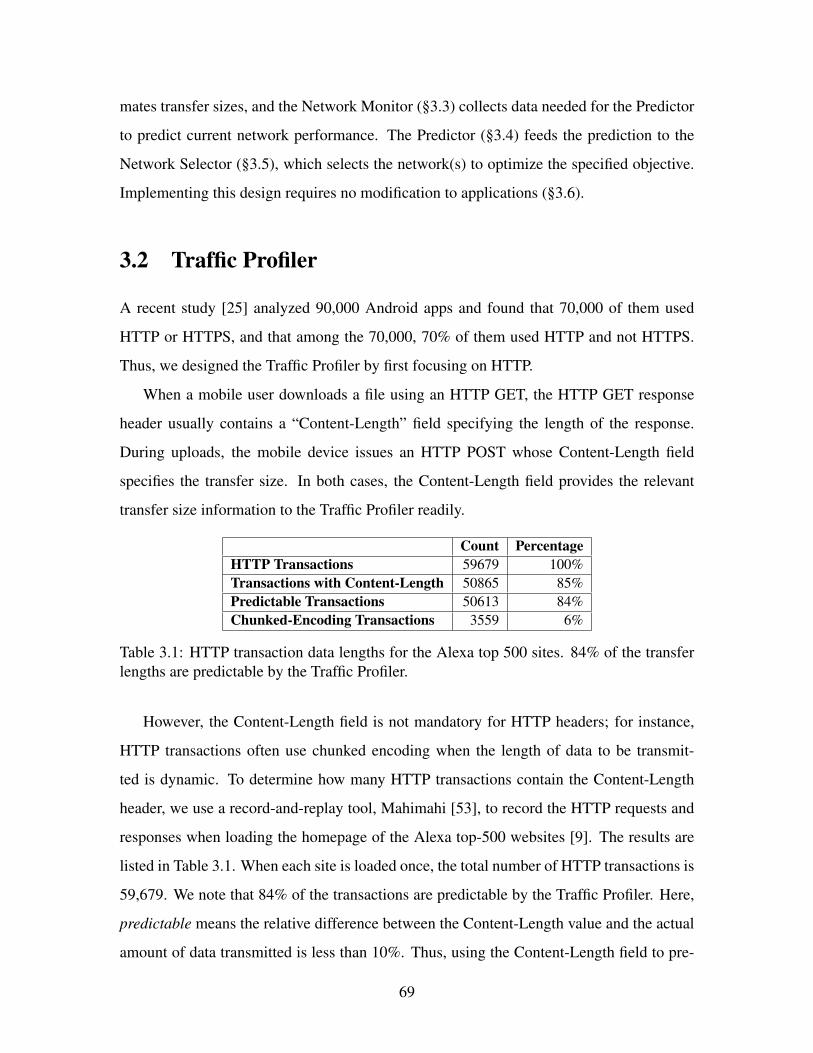
mates transfer sizes, and the Network Monitor (§3.3) collects data needed for the Predictor
to predict current network performance. The Predictor (§3.4) feeds the prediction to the
Network Selector (§3.5), which selects the network(s) to optimize the specified objective.
Implementing this design requires no modification to applications (§3.6).
3.2 Traffic Profiler
A recent study [25] analyzed 90,000 Android apps and found that 70,000 of them used
HTTP or HTTPS, and that among the 70,000, 70% of them used HTTP and not HTTPS.
Thus, we designed the Traffic Profiler by first focusing on HTTP.
When a mobile user downloads a file using an HTTP GET, the HTTP GET response
header usually contains a “Content-Length” field specifying the length of the response.
During uploads, the mobile device issues an HTTP POST whose Content-Length field
specifies the transfer size. In both cases, the Content-Length field provides the relevant
transfer size information to the Traffic Profiler readily.
Count PercentageHTTP Transactions 59679 100%Transactions with Content-Length 50865 85%Predictable Transactions 50613 84%Chunked-Encoding Transactions 3559 6%
Table 3.1: HTTP transaction data lengths for the Alexa top 500 sites. 84% of the transferlengths are predictable by the Traffic Profiler.
However, the Content-Length field is not mandatory for HTTP headers; for instance,
HTTP transactions often use chunked encoding when the length of data to be transmit-
ted is dynamic. To determine how many HTTP transactions contain the Content-Length
header, we use a record-and-replay tool, Mahimahi [53], to record the HTTP requests and
responses when loading the homepage of the Alexa top-500 websites [9]. The results are
listed in Table 3.1. When each site is loaded once, the total number of HTTP transactions is
59,679. We note that 84% of the transactions are predictable by the Traffic Profiler. Here,
predictable means the relative difference between the Content-Length value and the actual
amount of data transmitted is less than 10%. Thus, using the Content-Length field to pre-
69
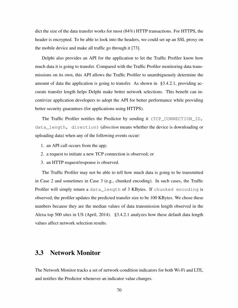
dict the size of the data transfer works for most (84%) HTTP transactions. For HTTPS, the
header is encrypted. To be able to look into the headers, we could set up an SSL proxy on
the mobile device and make all traffic go through it [73].
Delphi also provides an API for the application to let the Traffic Profiler know how
much data it is going to transfer. Compared with the Traffic Profiler monitoring data trans-
missions on its own, this API allows the Traffic Profiler to unambiguously determine the
amount of data the application is going to transfer. As shown in §3.4.2.1, providing ac-
curate transfer length helps Delphi make better network selections. This benefit can in-
centivize application developers to adopt the API for better performance while providing
better security guarantees (for applications using HTTPS).
The Traffic Profiler notifies the Predictor by sending it (TCP_CONNECTION_ID,
data_length, direction) (direction means whether the device is downloading or
uploading data) when any of the following events occur:
1. an API call occurs from the app;
2. a request to initiate a new TCP connection is observed; or
3. an HTTP request/response is observed.
The Traffic Profiler may not be able to tell how much data is going to be transmitted
in Case 2 and sometimes in Case 3 (e.g., chunked encoding). In such cases, the Traffic
Profiler will simply return a data_length of 3 KBytes. If chunked encoding is
observed, the profiler updates the predicted transfer size to be 100 KBytes. We chose these
numbers because they are the median values of data transmission length observed in the
Alexa top 500 sites in US (April, 2014). §3.4.2.1 analyzes how these default data length
values affect network selection results.
3.3 Network Monitor
The Network Monitor tracks a set of network-condition indicators for both Wi-Fi and LTE,
and notifies the Predictor whenever an indicator value changes.
70

Category Wi-Fi Indicators LTE IndicatorsPassive indi-cators
RSSI, Link Speed,Wi-FiAP Count
Signal Strength, DBM, RSSNR, CQI,RSRP,RSRQ, Wi-Fi AP Count
Active prob-ing
Max/Min/Mdev Ping RTT, DNS Lookup Time, UDP throughput, UDP loss-rate, UDP packet inter-arrival-time mean/median/90th percentile
Table 3.2: Network indicators monitored by Delphi.
3.3.1 Network Indicators
Table 3.2 lists the indicators used by Delphi. These indicators are categorized into 2 sub-
groups: passive measurement and active probing. The passive measurements capture chan-
nel quality and contention for the last-hop wireless link, which is often the bottleneck along
both the forward and reverse paths between the mobile device and the Internet. However,
this last-hop information does not always reflect network conditions along the whole path.
For example, for LTE networks, the delay introduced by packet buffering at the cell tower
side can be significant [35], but it is not captured by last-hop passive measurements. Wi-Fi
access in public areas such as shopping malls, airports, etc. may be subject to bandwidth
limits introduced at the gateway to the Internet, and these are not captured by last-hop
measurements. To capture these non-last-hop, or end-to-end network performance factors,
Delphi also runs active probes between the mobile device and an Internet server (see §3.6).
To quantify how each indicator affects TCP throughput, we analyze data collected from
22 locations. Those locations included shopping malls, Wi-Fi-covered downtown areas,
and university campuses, where both Wi-Fi and LTE were available. At each location,
the total measurement time is at least 1 hour. We compute the Pearson Correlation [75]
between the throughput and each indicator. The correlation is a number between −1 and
+1, inclusive. A value close to +1 or −1 signifies a strong positive or negative correlation.
A value close to 0 signifies weak correlation.
Figure 3-2 shows the absolute value for correlation between throughput and each indi-
cator. The bars in each sub-figure are sorted from strongest to weakest correlation. Fig-
ures 3-2a and 3-2b show the correlation over the entire dataset. For both Wi-Fi and LTE,
among the most correlated indicators, we see both active probing indicators (such as Wi-Fi
UDP throughput and LTE Average Ping RTT) and passive indicators. Figures 3-2c and 3-2d
71

0
0.2
0.4
0.6
0.8
1.0
Wi-F
i-udp
-tput
Wi-F
i-rss
i
Wi-F
i-links
peed
Wi-F
i-max
-ping-
rtt
Wi-F
i-mde
v-ping
-rtt
file-
size
Wi-F
i-avg
-ping-
rtt
Wi-F
i-dns
-look
-up-
time
Wi-F
i-udp
-IAT-9
0-pe
rcen
tile
Wi-F
i-min-p
ing-
rtt
Wi-F
i-ava
ilable-
coun
t
Wi-F
i-udp
-loss
rate
Wi-F
i-udp
-IAT-m
ean
Wi-F
i-udp
-IAT-m
edian
ab
s(C
orr
ela
tio
n)
Indicator Name
(a) Wi-Fi: All Data
0
0.2
0.4
0.6
0.8
1.0
LTE-a
vg-p
ing-
rtt
LTE-m
in-p
ing-
rtt
LTE-u
dp-tp
ut
file-
size
LTE-d
ns-lo
ok-u
p-tim
e
LTE-m
ax-p
ing-
rtt
LTE-s
s
LTE-m
dev-
ping
-rtt
LTE-u
dp-IA
T-90-
perc
entile
LTE-rs
snr
LTE-c
qi
LTE-u
dp-IA
T-med
ian
Wi-F
i-ava
ilable-
coun
t
LTE-u
dp-lo
ssra
te
LTE-rs
rq
LTE-u
dp-IA
T-mea
n
LTE-d
bm
ab
s(C
orr
ela
tio
n)
Indicator Name
(b) LTE: All Data
0
0.2
0.4
0.6
0.8
1.0
Wi-F
i-udp
-IAT-9
0-pe
rcen
tile
Wi-F
i-udp
-IAT-m
ean
Wi-F
i-udp
-tput
Wi-F
i-links
peed
Wi-F
i-min-p
ing-
rtt
Wi-F
i-avg
-ping-
rtt
Wi-F
i-max
-ping-
rtt
Wi-F
i-mde
v-ping
-rtt
file-
size
Wi-F
i-udp
-IAT-m
edian
Wi-F
i-dns
-look
-up-
time
Wi-F
i-rss
i
Wi-F
i-ava
ilable-
coun
t
Wi-F
i-udp
-loss
rate
ab
s(C
orr
ela
tio
n)
Indicator Name
(c) Wi-Fi: Location 1
0
0.2
0.4
0.6
0.8
1.0
Wi-F
i-links
peed
Wi-F
i-udp
-IAT-m
ean
file-
size
Wi-F
i-udp
-tput
Wi-F
i-dns
-look
-up-
time
Wi-F
i-udp
-IAT-m
edian
Wi-F
i-min-p
ing-
rtt
Wi-F
i-rss
i
Wi-F
i-mde
v-ping
-rtt
Wi-F
i-udp
-IAT-9
0-pe
rcen
tile
Wi-F
i-udp
-loss
rate
Wi-F
i-avg
-ping-
rtt
Wi-F
i-ava
ilable-
coun
t
Wi-F
i-max
-ping-
rtt
ab
s(C
orr
ela
tio
n)
Indicator Name
(d) Wi-Fi: Location 2
Figure 3-2: Correlation between Wi-Fi/LTE single path TCP throughput and each indicator.
show the correlation values calculated using data collected at only one location. Compared
to Figure 3-2a, at each location, the order of the correlation strength changes. Similar
results can be seen in LTE and MPTCP analysis.
3.3.2 Adaptive Probing
As shown in Figure 3-2, actively probing the network can provide important information
to estimate network performance. However, active probing can be expensive in terms of
energy, bandwidth, and delay. Table 3.3 summarizes the overhead in terms of delay, amount
of data transferred, and energy consumption.
To reduce the probing overhead, the Network Monitor probes the network adaptively,
only if there is a significant change in the passive indicators. Otherwise, it will reuse ac-
tive probing information collected previously. To further reduce probing overhead, Delphi
72

Probe Type DNS Query 10 Pings UDPData Transferred (Bytes) 271 1K 200KWi-Fi Median Delay (Sec) 0.64 9.02 0.65Wi-Fi Energy (mJ) 331 4730 366Cellular Median Delay (Sec) 0.63 9.01 0.58Cellular Energy (mJ) 1378 19697 1613
Table 3.3: Overhead for one occurrence of active probing. The delay values are the me-dian value across all measurement data collected at 22 locations. The energy values aremeasured in an indoor setting. The cellular energy values do not contain tail-energy [26].
adaptively probes only when the mobile device’s screen is on, which suggests that the user
is currently interacting with the device and is more sensitive to network delays. There are,
of course, times when background applications also need low delays (e.g., a cloud-based
navigation app), but in the common case, delay is less of a concern in such situations.
For background transmissions, Delphi will probe the network only when these two condi-
tions occur: 1) there is a large change in the passive measurements; and 2) there is a data
transmission request.
Adaptive probing has two benefits:
1. It is more energy-efficient than with fixed-rate probing.
2. It is proactive compared with probing only on a transmission request, which would
delay the request.
To evaluate adaptive probing, we simulate it using our collected data as follows. At
each location, we collected data from a series of runs measured back to back. We take the
first run’s passive and active measurement as input. Then, for the second run, we compare
the passive measurement values with the first run. If the passive measurement difference
d is less than a certain threshold T h, we keep the first run’s active probing values as our
measured number and use the second run’s active probing values as the ground truth to
calculate an error e. If d is greater than T h, we do active probing again.
The definitions of d and e for a run r are:
dr =m
∑i=1
|pi,r − pi,r−1|pi,max − pi,min
(3.1)
73

0
0.2
0.4
0.6
0.8
1
0.5 1 2 4 8 16 32 64 128 256 0
0.2
0.4
0.6
0.8
1
1.2
1.4
1.6A
ctive
Pro
bin
g F
req
ue
ncy
Active
Pro
bin
g E
rro
r
Adaptive Probing Threshold (10-4
)
Wi-Fi ErrorLTE Error
Probing Frequency
Figure 3-3: As the adaptive probing threshold (x-axis) increases, the number of probingdecreases and the probing error increases. Here the left y-axis shows the probing frequency,which is the average number of probing in every five minutes.
er =n
∑j=1
|a j,r −a j,r|a j,r
(3.2)
Here, m is the total number of passive indicators; pi is the value of the passive indicator
i; pi,max and pi,min are the max and min values for these indicators; n is the total number of
active indicators; a j,r is the active probing value for indicator j, and a j,r is the ground truth
value in run r.
Figure 3-3 shows that as the probing threshold increases, fewer probes are triggered.
Also, as the probing threshold increases, the error of reusing the previous active probing
value increases. In §3.4, we will analyze the extent to which the choice of network is
affected by this adaptive probing error.
74

3.4 Predictor
Delphi’s Predictor takes the traffic profile and network status as input to estimate network
performance. In this section, we focus on how it estimates TCP flow completion time
because flow completion time is used in all our objectives mentioned in §3.5. However,
similar techniques can be used to estimate other metrics such as average throughput (for
streaming applications) or average RTT (for interactive applications).
To predict TCP flow completion time, or related metrics such as the end-to-end through-
put for Wi-Fi and LTE networks, previous work either uses historical data from the same
flow to predict current throughput [78], or it outputs binary results such as high/low through-
put [22]. However, for Delphi, the prediction is more challenging: First, it needs to make
its decision just before the connection transfers data, and recent historical data may not
always available. Second, it needs to return numerical values instead of binary results to be
fed into the Selector.
We use a machine learning model, the regression tree [56], to estimate TCP flow com-
pletion time. This learning method matches well with our problem definition, as it takes
multi-dimensional vectors as input and produces a real-valued result. In our case, the multi-
dimensional input includes data size and network condition indicators. Another advantage
of using a regression tree is that by assigning different weight to different indicators when
traversing through different branches, per-location differences (Figure 3-2) are captured
naturally. Regression trees have been used to solve other network performance estimation
problems [78] due to their low memory and computation overhead.
Delphi constructs four regression trees to predict the flow completion time for single-
path TCP over Wi-Fi or LTE, and for MPTCP using Wi-Fi or LTE for the primary subflow.
We estimate the flow completion time of MPTCP using separate trees instead of deriving it
from the flow completion time estimated for single-path TCP because a previous measure-
ment study [27] shows that throughputs of single-path TCP over two networks do not add
up to the throughput of MPTCP. Besides, there are cases where MPTCP over both networks
gives lower throughput than single-path TCP over a single network does.
The prediction accuracy is affected by two factors:
75

0
0.25
0.5
0.75
1.0
0 0.1 0.2 0.3 0.4 0.5
CD
F
Relative Error
Tree
SVR
(a) TCP over Wi-Fi
0
0.25
0.5
0.75
1.0
0 0.1 0.2 0.3 0.4 0.5
CD
F
Relative Error
Tree
SVR
(b) TCP over LTE
Figure 3-4: Relative error when using the regression tree and support vector regression tolearn the flow completion time. The line marked with “Tree” shows the relative error of theregression tree model. The line with “SVR” shows the relative error of the support vectorregression model.
1. the predictive power of the machine learning model, that is, whether regression trees
are a good model for predicting flow completion time, and
2. the measurement accuracy of the inputs to the machine-learning methods.
3.4.1 Regression Tree Prediction Accuracy
Here, we use our dataset collected from 22 locations to analyze Delphi’s prediction accu-
racy. To train the regression tree model, we randomly select 10% of the total samples from
our dataset. We then use the remaining 90% as our testing data. As a comparison, we also
train support vector regression (SVR) models with the radio basis kernel [60], which also
takes a multi-dimensional vector as input and produces numerical results. The SVR mod-
els also consist of four separate models, each for one network configuration. To train each
SVR model, we first sort all the indicators from the most correlated to the least correlated
with the flow completion time. Here, we compute the correlation across all the data, not
just the 10% in the training set, so that the sorting will not be biased by the training set.
Then, we train the SVR model using the N most correlated features. As N increases, the
testing errors first decrease (because the model improves in predictive power) and then in-
crease (because the model overfits to the training set). For each SVR model, we choose the
N that gives the smallest error. Thus, the resulting models are the best that can be achieved
76

0
0.1
0.2
0.3
0.4
0.5
0.6
0.7
0.8
0.9
1
0 0.2 0.4 0.6 0.8 1
CD
F
Relative Error
2 KB
5 KB
10 KB
100 KB
1 MB
Figure 3-5: Relative error when using an empirical flow size number (3 KBytes) to predictflow completion time. The legends are the actual flow sizes.
using the SVR method given the features that we measure.
We test both models using the same testing set. Figure 3-4 shows the CDF of relative
error between the learned result and the ground truth when predicting Wi-Fi and LTE.
MPTCP predictions give similar results. Here, the regression tree model predicts the flow
completion time with smaller error than the SVR model. Regression tree is more powerful
because it is able to traverse through different paths in the tree when predicting different
locations.
The median testing error ranges from 2% to 10% across the four regression tree mod-
els. Given that the training set consists of only 10% of the data, this shows the TCP flow
completion time is predictable using regression trees.
3.4.2 Input Error Analysis
§3.4.1 shows the prediction error when the input feature vectors are accurate. As described
earlier, the Traffic Profiler sometimes needs to guess the transfer size, and the Network
Monitor may reduce active probing frequency to reduce energy and traffic overhead. Thus,
the input to the regression tree is not always perfect. In this section, we investigate what
77

0
0.1
0.2
0.3
0.4
0.5
0.6
0.7
0.8
0.9
0 0.05 0.1 0.15 0.2 0.25 0.3 0.35 0.4
CD
F
Relative Error
Th=0
Th=0.0001
Th=0.0002
Th=0.0004
Th=0.0008
Th=0.0016
Th=0.0032
Passive
Figure 3-6: Relative error when using adaptive probing to predict flow completion time.
impact these imperfections have.
3.4.2.1 Traffic Profiler Error
As mentioned in §3.2, when there is no Content-Length field specified in a burst of trans-
mission, the Traffic Profiler returns an empirical number of 3 KBytes. Figure 3-5 shows the
relative error using an inaccurate transfer size as a regression tree’s input (in Figure 3-5, we
show only the results for TCP over LTE for clarity, but similar results hold for Wi-Fi and
MPTCP). Here, we split the testing dataset into smaller subsets; each subset contains mea-
surement done for a certain transfer size. As the difference between the actual transfer size
and 3 KBytes increases, the relative error increases. The prediction error is significantly
higher than the previous 2%-10%. Fortunately, however, only less than 15% of transfers
are affected by this error, as noted in §3.2.
3.4.2.2 Network Monitor Error
Another source of error is adaptive probing. We run the regression tree testing over different
T h values, which is an adaptive probing parameter. Figure 3-6 shows the CDF curves of
78

relative errors for LTE. Here, as T h increases (i.e., probing less frequently), the prediction
error increases. Wi-Fi and MPTCP predictions also gives similar results.
3.5 Network Selector
Delphi’s Selector uses network performance predictions, transfer lengths, and the speci-
fied objectives for application transfers to determine which network to use. The choice of
network depends on three factors: throughput, energy efficiency, and monetary cost.
3.5.1 Objective Functions
Throughput, S: The Selector can estimate the average throughput of the current transfer
using the transfer size f that is provided by the Traffic Profiler and the flow completion
time t that is provided by the Predictor. Using the subscript i to refer to the choice of the
network (either Wi-Fi or LTE or MPTCP with a specified primary subflow), we have:
Si =fti
(3.3)
Energy per byte, Ei: Knowing the power level pi of each network choice i, together
with the above ti and f , the energy to transmit one byte is:
Ei =pi · ti
f(3.4)
The energy per byte is a metric that captures both battery consumption and transfer
rate. A faster transfer over a network that has a higher power consumption may incur lower
energy per byte. As a result, minimizing energy per byte is not always the same as picking
the network with the lowest power consumption.
Monetary cost per byte, Mi: The “dollar” cost incurred when transferring each byte
of the transfer on network choice i.
By knowing Si, Ei, and Mi, the Selector chooses the network that maximizes the fol-
lowing objective function:
79

Oi =Si
α
Eiβ ·Mi
γ(3.5)
This objective function prefers networks with high Si values, meaning in a given second,
it wants the device to transfer more bytes. It also prefers networks with low Ei value,
meaning when consuming one joule of energy, it wants the device to transfer more bytes.
Similarly, it prefers networks with low Mi values, meaning when consuming one dollar, it
wants the device to transfer more bytes.
The exponents α , β , γ ∈ [0,∞) determine the relative importance of throughput, energy
efficiency, and monetary cost, respectively. For example, if α = 1, β = 0, and γ = 0,
then Oi = Si, and the Selector will select the network with the highest average throughput.
This optimization is realistic if the device has an unlimited data plan and is connected to
an AC power source. As another example, if α = 0, β = 1, and γ = 0, then Oi = 1/Ei ,
and the Selector will select the network that consumes the least amount of energy. This
optimization is preferable when the device is about to run out of battery.
In our experiments, we set α , β , γ to different values to experiment with different
scenarios. In a more realistic implementation, α , β , and γ can be pre-defined by users or
decided by Delphi dynamically according to the phone’s current status. For example, β
can increase as the battery level decreases. If the mobile device user has a limited monthly
data plan for a cellular network, γ can increase as the amount of data plan consumed is
approaching the budget, and set at a large number once the cellular usage exceeds the
budget. Picking different values of α , β , and γ makes the objective function expressive
enough to handle a range of preferences.
3.5.2 Energy Model
An energy model is required to estimate Ei. We measured the power level of both Wi-Fi
and LTE on a Galaxy Nexus phone by connecting it to a power monitor [43]. We measured
the power level during both TCP uploads and downloads using Wi-Fi and LTE. We also
measured the power level across different transmission rates for both Wi-Fi and LTE, by
changing the underneath channel quality. To do so, for Wi-Fi, we change the distance
80

Interface LTE Wi-FiSend Tput (mbps) 2.3∼4.4 7.4∼9.4Send Power (mW) 2778±56 536±23Recv Tput (mbps) 0.1∼1.5 7.3∼9.5Recv Power (mW) 1674±95 428±58
Table 3.4: Power level measurement for Wi-Fi and LTE in a indoor setting. The Wi-Fipower is measured when the mobile device is associated with an AP deployed inside thebuilding. The LTE power is measured when the mobile device is connected to Verizon LTEnetwork.
between the phone and the access point. For LTE, we change the channel quality by moving
into and out of buildings.
Table 3.4 shows the results. For each network, both while uploading and downloading
data, the power level stays the same regardless of the data rate. Hence, we model the power
pi for each network using two constant numbers (one for upload and one for download).
However, for LTE, there is an additional tail energy [26] component that is consumed after
a transfer finishes, which we treat as a constant number. As a result, when estimating the
energy consumed for LTE, Delphi adds this tail energy to the total energy consumed.
3.5.3 Selector Performance
To quantify the Selector’s performance, we run simulations using data that we collected
from 22 locations. We wrote a simulator that operates on this data set as described below.
The dataset collected earlier maps a feature vector (made up of all the features listed in
Table 3.2) to a tcpdump trace captured when running standard TCP on Wi-Fi and LTE
and a tcpdump trace for MPTCP in striped mode using Wi-Fi as the primary subflow and
using LTE as the primary subflow.
When evaluating any scheme, we assume all the features required by Delphi are avail-
able at the beginning of each run. We run Delphi’s selection algorithms, described earlier,
using the features collected at the beginning of the run along with flow size as input. We
then pick the network interface that maximizes the objective function described above and
look at the previously collected tcpdump trace to determine the duration from the begin-
ning of the trace until a transfer size worth of bytes are transferred. We repeat the same
81

0
1
2
3
4
0 2 4 6 8 10
Thro
ughp
ut (M
Bits
/Sec
)
Energy Efficiency (MBits/J)
Max(S)
Max(S/E)
Wi-FiLTEMPTCP(Wi-Fi)
MPTCP(LTE) Oracle Frontier
Figure 3-7: Megabits per joule and throughput values for different schemes. The black lineshows a frontier of the best median values that can be achieved when setting α = 1, γ = 0and changing β from 0 to 5. For each scheme, the black dot shows the median value andthe ellipse shows the 30th and 70th percentiles.
procedure, without any prediction, for the other policies for every run at each location.
In these simulations, we set γ = 0, meaning we do not consider monetary cost. Figure 3-
7 shows the simulation results. The x-axis of the figure shows the number of bits that can
be transmitted when consuming one joule. The y-axis shows the throughput. We first draw
a frontier line by changing β from 0 to 5. When computing the frontier, we also use the
ground-truth value of each flow’s completion time so that the frontier represents the best
that can be achieved if we have a perfect predictor. We call this line “Oracle Frontier”.
In Figure 3-7, Wi-Fi, LTE, MPTCP(Wi-Fi), and MPTCP(LTE) are four fixed schemes
where the same network is used across all locations. Here, Wi-Fi and LTE refer to trans-
mitting data using single-path TCP over Wi-Fi or LTE. MPTCP(Wi-Fi) and MPTCP(LTE)
refer to transmitting data over MPTCP, while using Wi-Fi or LTE for primary subflow.
“Max(S)” and “Max(S/E)” are two schemes run by the Selector. In Figure 3-7, the two
Delphi schemes, Max(S) and Max(S/E), fall close to the frontier line. In Max(S), the Se-
lector set β = 0, meaning it is simply trying to maximize throughput. In Max(S/E), β = 1,
82

0
0.25
0.5
0.75
1.0
OracleDelphi
OracleDelphi
OracleDelphi
Se
lecte
d R
atio
LTEWi-FiMPTCP(LTE)MPTCP(Wi-Fi)
Max(1/E)Max(S/E)Max(S)
Figure 3-8: Percentage of each network(s) is selected when using different objective func-tions.
meaning it tries to select networks with high throughput but without consuming too much
energy. We can see that Max(S) and Max(S/E) are much closer to the Oracle Frontier line
than any other schemes are.
Objective Max(S) Max(S/E) Wi-FiThroughput (Mbits/Sec) 3.0 2.6 1.4Energy Efficiency (Mbits/J) 2.8 4.9 5.2
Table 3.5: Median values for Max(S), Max(S/E) and Wi-Fi as shown in Figure 3-7.
Table 3.5 lists the x and y-axis median values for Max(S) and Max(S/E), together with
the median value for the fixed scheme that always uses Wi-Fi for comparison. Here, Max(S)
gives the highest median throughput of 3.0 Mbit/s, which is a 2.1× gain over Wi-Fi’s 1.4
Mbit/s. Max(S/E) tries to achieve high throughput with high energy efficiency. Its median
energy efficiency is 4.9 Mbit/J, 6% worse than always using Wi-Fi, but it achieves a median
throughput of 2.6 Mbit/s, a 1.9× gain over Wi-Fi.
We now take a closer look at each scheme. When an objective function is defined, how
many times is each available choice selected? Figure 3-8 shows the percentage of time that
each network choice is selected when trying to optimize different objectives. First, we can
83

0
20
40
60
80
100
Max(S/E) Max(S)
Su
cce
ss R
ate
(%
)
ActiveAdaptivePassive3 KB
Figure 3-9: Success rate for different schemes.
see that Delphi makes very similar decisions compared with an omniscient oracle. How-
ever, for each specific objective function, Delphi chooses different networks. For exam-
ple, when maximizing throughput, Delphi selects LTE more often than Wi-Fi or any other
MPTCP-based scheme because LTE provides the highest throughput in a large number of
cases in our dataset. For Max(S/E) (maximizing throughput over energy) or for Max(1/E)
(minimizing energy consumption), Delphi tends to choose Wi-Fi much more often, since
Wi-Fi is generally more energy-efficient. However, both the oracle and Delphi still select
other network(s) because there are cases where Wi-Fi gives really low throughput, length-
ening the transfer and consuming significant energy in the process.
To understand these errors in more detail, we compare the decision made by the oracle
and by Delphi. We say that Delphi makes a successful decision if it selects the same
network(s) as the oracle. Figure 3-9 shows the ratio of successful decisions affected by
different error sources. Here, “Active” refers to using active probing information for flow-
completion time prediction. “Adaptive” refers to our adaptive probing technique described
earlier. “3 KB” refers to using active probing, in which the Traffic Profiler outputs 3 KBytes
in 16% of the total outputs. We selected 16% because we found that in 16% of the total
network transactions data size is not predictable (Table 3.1 in §3.2).
84

We can see that Active gives the highest success ratio (93% for Max(S/E) and 85% for
Max(S)). As we add error to the network measurement input, or Adaptive, the success ratio
is lower (90% and 81%, respectively). Finally, inaccurate transfer size information gives
us the lowest success rate (86% and 78%, respectively). These results show that we can
achieve high success rates by adding active probing overhead. If the overhead is a concern,
removing active probing can still give reasonable results. However, being able to predict
the size of the burst of traffic is more important.
3.5.4 System Generalization
Model Type Obj. Throughput(Mbits/Sec)
Energy Efficiency(Mbits/J)
SVR Max(S) 2.3 1.6Reg. Tree Max(S) 2.1 2.0Wi-Fi Only - 1.4 5.6LTE Only - 1.7 1.5SVR Max(S/E) 1.4 5.6Reg. Tree Max(S/E) 1.9 2.7
Table 3.6: Median values for throughput and energy efficiency when testing different mod-els at new locations.
In our above analysis, both our training and testing datasets are generated from the 22
locations we measured. These results show the improvement when we have prior knowl-
edge of the network condition of each location. In this section, we show the results in a
more challenging condition: we test Delphi’s performance when there is no prior knowl-
edge. This corresponds to the real use case when a smartphone user enters a new location
that he or she has never been to.
We trained Delphi using data collected from 21 out of the 22 locations and tested it
on the last location. We repeated this process 22 times by using each location to be the
testing set. Table 3.6 shows that when maximizing throughput, Delphi achieves up to 1.6×
improvement (when using the SVR model) over Wi-Fi. When maximizing throughput over
energy consumption, Delphi behaves as well as Wi-Fi and better than using LTE only.
These results show that 1) when there is no prior knowledge, the improvement decreases,
and 2) the SVR model achieves higher improvement than the regression tree does. This is
85

because the regression tree is powerful when it characterizes data in a training set, which
means it tends to overfit, and is less powerful when predicting new data. Thus, Delphi
can use the SVR model to make decisions when entering new locations, or crowd-sourcing
measurement techniques [68] can be used to feed the smartphone with prior knowledge of
new locations to further improve performance.
3.6 Implementation
We implemented Delphi on a laptop (2.4GHz Dual Core with 4GB RAM, comparable to
a smartphone) running MPTCP (Ubuntu Linux 13.10 with Kernel version 3.11.0, with the
MPTCP Kernel implementation version v0.88 [51]). We tethered two smartphones to the
laptop, one in airplane mode with Wi-Fi enabled and the other with Wi-Fi disabled but
connected to the Verizon LTE network. The reason we implemented Delphi on a laptop
instead of a smartphone is to utilize existing machine learning libraries. We also enabled
MPTCP on a Galaxy Nexus phone running Android 4.1 [48] to validate that all the follow-
ing functionality is feasible on smartphones. All the measurement data used for simulation
in the previous settings are also collected under the same setting.
The current implementation of Delphi is a user-level application implemented in Python.
One thread of Delphi serves as the Network Monitor; it continuously polls passive indicator
values from both phones over the USB interface every 500 milliseconds.
Switch Type Send Delay (ms) Recv Delay (ms)LTE switch on 494± 1 507 ± 13Wi-Fi switch on 495 ± 2 782 ± 47
Table 3.7: Switching delay, averaged across 10 measurements. The switching delay isdefined as the time between an iptable rule-changing command being issued and apacket transfer occurring on the newly brought-up interface. The send delay is the delayfor the first out-going packet showing up, and the receive delay is for the first ACK packetcoming from the server.
The other thread serves as the Traffic Profiler, Predictor, and Selector. It runs tcpdump
to monitor packet transmissions in real time. Once it sees that a network transfer has been
initiated, it looks for an HTTP request or response header and reads the Content-Length
86

information from the header. It then calls the Predictor function to predict the transfer
completion time and then calls the Selector function to select a single network by changing
iptable rules [50]. This procedure of turning an interface off allows MPTCP to migrate
to the new connection because it supports break-before-make semantics. When the network
is idle, this thread also reads the passive indicator values periodically (every 5 seconds), and
uses a default value of 3 KBytes as transfer length when calling the Predictor and Selector
functions so that the network can be pre-selected before a new TCP connection starts. When
a connection is actively transmitting, Delphi also periodically (every 500 milliseconds)
reads the passive indicator values so that it can detect significant network environment
changes in case the mobile device is moving. This allows Delphi to dynamically select
networks during long-running transfers. Once the Selector decides an interface switching
is required, it achieves the switch by changing iptable entries for that specific TCP
connection. Table 3.7 shows the interface switching delay measured in an indoor setting.
Each number is an average across 10 measurements. The switching delay is defined as
the time between an iptable rule-changing command being issued and a packet transfer
occurring on the newly brought-up interface. In our current implementation, the out-going
delay is 500 ms. During this 500 ms, the transfer does not pause but continues on the pre-
selected network. Notice that not all connections will experience this delay because Delphi
can pre-select the network configurations as it observes a network condition change. This
switch delay will happen only when 1) the network condition changes during a transfer
or 2) the network selection result based on the actual transfer size is different from the
result based on the default 3 KBytes value. In our experiments (§3.7.2), 18% of HTTP
transactions incur a network switch during data transfer.
We configured the laptop to pass all its HTTP traffic through an MPTCP-enabled proxy
server. Because current app servers do not always support MPTCP, the proxy server allows
our client to run apps over MPTCP while talking to the apps’ original server.
87

0
0.25
0.5
0.75
1.0
Max(S) Max(S/E)
No
rma
lize
d O
bj.
Wi-FiLTEMPTCP(Wi-Fi)MPTCP(LTE)Delphi
(a) Web Browsing
0
0.25
0.5
0.75
1.0
Max(S) Max(S/E)
No
rma
lize
d O
bj.
Wi-FiLTEMPTCP(Wi-Fi)MPTCP(LTE)Delphi
(b) Video Streaming
Figure 3-10: Objective function value normalized by oracle. The histogram shows themedian value; the error bar shows 20th and 80th percentiles.
3.7 Evaluation
In previous sections, we analyzed the performance of each module using a trace-driven
approach. This serves as a micro-benchmark evaluation of Delphi. In this section, we
focus on macro-benchmark evaluation done by emulation and real-world experiments.
3.7.1 Delphi Over Emulated Networks
To understand Delphi’s performance under real application workloads, we used Mahimahi,
a record-and-replay tool that can record and replay client-server interactions over HTTP [53].
In our experiment, we recorded client-server interactions when the client ran two applica-
tions: web browsing and video streaming. During replay, Mahimahi replays the recorded
interactions on top of an emulated network. Mahimahi can emulate network delays and
variable-rate links using packet-delivery traces. In our experiment, we used the tcpdump
traces captured during our measurement at 22 locations as packet-delivery traces for net-
work emulation. During the tcpdump measurements, we also measured passive indicator
values, which were fed into Delphi during our emulation as inputs to the Network Moni-
tor. This emulation setup enabled us to compare different network selection schemes when
running exactly the same application traffic and under the same network conditions.
We used Delphi to optimize two different objective functions, 1) Max(S): maximizing
average throughput (i.e. minimizing transfer completion time) and 2) Max(S/E): max-
88
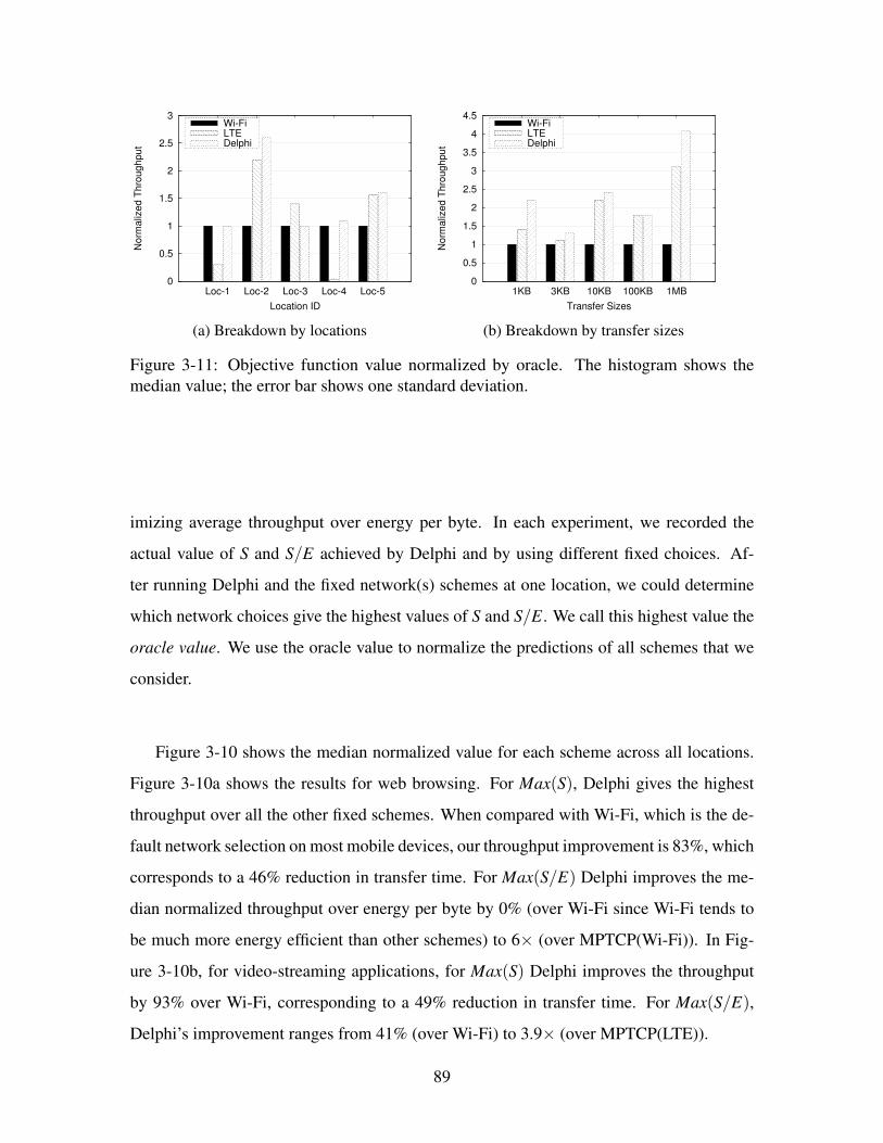
0
0.5
1
1.5
2
2.5
3
Loc-1 Loc-2 Loc-3 Loc-4 Loc-5
No
rma
lize
d T
hro
ug
hp
ut
Location ID
Wi-FiLTEDelphi
(a) Breakdown by locations
0
0.5
1
1.5
2
2.5
3
3.5
4
4.5
1KB 3KB 10KB 100KB 1MB
No
rma
lize
d T
hro
ug
hp
ut
Transfer Sizes
Wi-FiLTEDelphi
(b) Breakdown by transfer sizes
Figure 3-11: Objective function value normalized by oracle. The histogram shows themedian value; the error bar shows one standard deviation.
imizing average throughput over energy per byte. In each experiment, we recorded the
actual value of S and S/E achieved by Delphi and by using different fixed choices. Af-
ter running Delphi and the fixed network(s) schemes at one location, we could determine
which network choices give the highest values of S and S/E. We call this highest value the
oracle value. We use the oracle value to normalize the predictions of all schemes that we
consider.
Figure 3-10 shows the median normalized value for each scheme across all locations.
Figure 3-10a shows the results for web browsing. For Max(S), Delphi gives the highest
throughput over all the other fixed schemes. When compared with Wi-Fi, which is the de-
fault network selection on most mobile devices, our throughput improvement is 83%, which
corresponds to a 46% reduction in transfer time. For Max(S/E) Delphi improves the me-
dian normalized throughput over energy per byte by 0% (over Wi-Fi since Wi-Fi tends to
be much more energy efficient than other schemes) to 6× (over MPTCP(Wi-Fi)). In Fig-
ure 3-10b, for video-streaming applications, for Max(S) Delphi improves the throughput
by 93% over Wi-Fi, corresponding to a 49% reduction in transfer time. For Max(S/E),
Delphi’s improvement ranges from 41% (over Wi-Fi) to 3.9× (over MPTCP(LTE)).
89

3.7.2 Experiments
To understand how Delphi behaves in the real world, we first trained Delphi’s predictor
using data we collected at the 22 locations. The model training was done using a desktop
(Intel Xeon(R) CPU, 3.30GHz Quad Core, 16 GB RAM). The total training process took
five minutes. Then, among the 22 locations, we visited five close to our campus. On
our Delphi-enabled laptop, we ran wget to download files with various sizes (1 KByte, 3
KBytes, 10 KBytes, 100 KBytes, and 1000 KBytes) from a remote server. For comparison,
we also ran the same wget with only Wi-Fi or LTE enabled before or after we ran Delphi.
We randomized the sequence of configurations (file sizes, network measured). For each
configuration, we ran it five times.
Figure 3-11 shows the average improvement of Delphi over Wi-Fi and LTE, when Del-
phi’s objective is set to maximize throughput. Due to high variation of the actual through-
put across different configurations, here we show the throughput normalized by Wi-Fi’s
throughput. Figure 3-11a shows Delphi’s performance at each location. We can see that
Delphi does not perform perfectly. At Location 3, the LTE had a higher average throughput
than Wi-Fi, but Delphi still selected Wi-Fi. However, at other locations, Delphi performed
better than always using Wi-Fi or LTE. At Locations 2, 4, and 5, Delphi performed better
than both Wi-Fi and LTE, because it used MPTCP running over both networks. In Figure 3-
11b, we can see that Delphi achieves improvement for small (1 KByte, 3 KBytes, and 10
KBytes) and large (100 KBytes) transfers. A deeper investigation reveals that the middle-
sized (1 MByte) transfers are affected by the switching delay (explained in §3.6) the most:
Most of the transfers go through the sub-optimal network(s). However, for large transfers,
although it also transfers on the sub-optimal network(s) for some time, most of the transfers
happen after the network switch. Thus, Delphi performs well for large transfers. In sum-
mary, Delphi increases average throughput by up to 4× compared with Android’s default
policy that always uses Wi-Fi when it is available.
90

0
1
2
3
4
5
6
0 10 20 30 40 50
Th
rou
gh
pu
t (M
bits/S
ec)
Lose IPDelphi Switch
DelphiWi-FiLTE
Delphi Cell PredictDelphi Wi-Fi Predict
Figure 3-12: When the mobile device is moving away from an access point, Delphi predictsthat Wi-Fi can be worse than LTE, then it switches to LTE at time 10.5 seconds. MPTCPhandover mode switches to LTE when it sees Wi-Fi loses the IP, which happens at time 41seconds.
3.7.3 Handling User Mobility
Another benefit of using Delphi is that by continuously monitoring the network conditions
using the Network Monitor, Delphi can tell whether the network performance is getting
worse and trigger handover proactively. This is best demonstrated when the mobile device
is moving. In this experiment, we kept Delphi running on the laptop while moving it from
inside a building to outside a building. The tethered Wi-Fi phone was initially connected
to the Wi-Fi AP inside the building. As we walked outside the building, the Wi-Fi signal
kept decreasing until the phone could not associate with the AP. We ran wget on the laptop
to download a large file from our proxy server. In this experiment, we configured Delphi
to Max(S) and to select only between Wi-Fi and LTE, not the MPTCP choices, to study
the handover behavior. In our experiment, We first ran wget without running Delphi, and
with only one interface at a time, to measure the throughput of Wi-Fi and LTE as the laptop
moved, shown as “Wi-Fi” and “LTE” in Figure 3-12. Then we ran Delphi while moving the
laptop along the same path. In Figure 3-12, we can see that at time 10.5, Delphi predicted
91

2
3
4
5
6
7
8
0 20 40 60 80 100 120 140 160
Tp
ut
(Mb
ps)
Time (Minutes)
Wi-Fi DownloadLTE Download
Figure 3-13: Wi-Fi and LTE download throughput at the same location over 2.5 hours.
that Wi-Fi was worse than LTE and consequently triggered a switch, and the throughput
dropped but soon recovered to LTE’s throughput. In Figure 3-12, we also marked the time
when the phone lost its Wi-Fi IP address; this is when a handover will happen according
to Multi-Path TCP Handover-Mode proposed in [57]. However, we can see that in this
case, Wi-Fi throughput had already dropped to zero before it lost the IP address. Compared
with this scheme, Delphi triggers LTE/Wi-Fi handover earlier so that the application sees
constantly high throughput.
3.8 Discussion
In this section, we discuss two alternative network selection schemes and compare them
with Delphi.
3.8.1 Purely Location-Based Algorithm
The first alternative algorithm is to use location information to make network selection
decisions. The assumption is that at certain locations, a mobile device tends to use a certain
92

0
2
4
6
8
10
12
Indoor Outdoor
Tp
ut
(Mb
ps)
Wi-FiLTE
Figure 3-14: Wi-Fi and LTE download throughput measured indoors and outdoors. Thebar shows the average throughput over 10 measurements; the error bar shows the standarddeviation.
network combination. However, we argue that network location is not the only dominant
factor. Figure 3-13 shows the measured Wi-Fi and LTE throughput at one location over a
period of 2.5 hours. We can see that both Wi-Fi and LTE throughput varies significantly
during this period of time. Wi-Fi has higher throughput than LTE does at certain time
points, while LTE has higher throughput than Wi-Fi has at other times. Thus, if the goal
is to select the network with the highest throughput, a purely location-based method is not
guaranteed to make the correct choice all the time.
Another challenge for using location as the network selection signature is to select a
proper granularity of location. Figure 3-14 shows the TCP throughput for Wi-Fi and LTE
measured at two nearby locations, one inside a building and one outside the building. The
distance between the two locations is about 20 meters. We can see that the throughput
changes dramatically between these two locations; thus, the network selection for maxi-
mizing throughput will also change. Moreover, as shown in the previous section, when
moving from indoors to outdoors, Delphi can detect the network condition change and
switch between networks accordingly. To make a location-based approach have similar
93

0
0.25
0.5
0.75
1.0
Web Video
No
rma
lize
d T
hro
ug
hp
ut
Wi-FiLTEDelphiRecent-best
Figure 3-15: Throughput normalized by oracle. The histogram shows the median value;the error bar shows the 20th and 80th percentiles. The bars labeled “Recent-best” show theresults for picking-the-recent-best.
capability, it needs to have location and network performance mappings within the granu-
larity of 20 meters or less. This requires intensive measurement done beforehand as well as
mobile devices having accurate localization capabilities both indoors and outdoors, which
can bring extra computational and energy overhead for the devices.
3.8.2 Picking the Recent-Best Choice
Another idea is to send traffic on each networks or network combinations then select the one
that gives the best performance for the rest of the data transfers. We applied this approach to
web traffic. A typical web page load consists of many small transfers (HTTP transactions);
thus, the first few transfers can be transferred on all available network combinations, and
then the rest of the transfers will be assigned to the best one according to the observed
performance. We compared this approach with Delphi. Figure 3-15 shows the results when
running both schemes to select the network with the highest average throughput. We find
that this picking-the-recent-best approach performs worse than Delphi does and even worse
than static approaches, in both web page loading and video streaming.
94

To understand why this picking-the-recent-best scheme performs poorly, we take a
deeper look into the results and find that for web page loading, whose traffic consists of
many short transfers, the total page load time is dominated by the probing phase to pick the
best choice because some data has to be transmitted on the slow network choices.
The video streaming traffic contains a few short transfers at the beginning, which are
used for probing. However, because different transfer sizes may result in different network
performances, a fast network for short transfers may not be a fast network for long transfers.
This probing-while-transferring approach ends up using a slower network for the main
video file downloading. In our experiment, for video streaming the success rate (selecting
the same network as oracle) for Delphi is 60%, and it decreases to 50% for picking-the-
recent-best.
3.9 Related Work
We discuss related work on mobile network selection policies, MPTCP, scheduling algo-
rithms that generalize processor sharing [59] to multiple interfaces, roaming mechanisms
to seamlessly migrate between interfaces, and systems and APIs that allow applications to
benefit from multiple interfaces.
3.9.1 Mobile Network Selection
Zhao et al. [84] present a system that picks from one of three choices for every flow: reg-
ular IP, mobile IP [62] with triangle routing, and mobile IP with bidirectional tunneling.
Instead of selecting an entire path within the Internet, as Zhao et al. do, Delphi picks ei-
ther an LTE link or a Wi-Fi link for the last hop alone. CoolSpots [61] and SwitchR [7]
address the question of network selection between Wi-Fi and Bluetooth networks available
on the phone. In contrast, Delphi chooses between Wi-Fi and LTE on the last hop using
different techniques. MultiNets [54] proposes a mechanism to allow smartphones to use
multiple networks based on certain policies, such as energy saving, data offloading, and
performance. However, MultiNets explicitly assumes that Wi-Fi is faster than the cellular
link is, which no longer holds true [27]. ATOM [42] is a traffic management system allocat-
95

ing mobile devices’ traffic between LTE and Wi-Fi networks operated by the same service
provider. ATOM’s selection decision was made at the service provider side in a centralized
way. However, Delphi is able to make selections across different Wi-Fi and LTE providers,
in a distributed approach, in which the mobile devices make the decision.
Theoretical work on this problem includes multi-attribute decision making [17], game
theory and reinforcement learning [55], and analytic hierarchy processes [72]. These are
primarily evaluated in simulation using simplified models of the network and workloads.
In contrast, our evaluation consists of trace-driven simulations and real-world experiments
with traffic from unmodified applications.
3.9.2 Multi-Path TCP
Multi-Path TCP (MPTCP) [77], and its recent implementation in iOS 7 [49] allow a single
TCP connection to use multiple paths. MPTCP does not specify if interfaces should be used
simultaneously or in master-backup mode. The iOS implementation operates in master-
backup mode using Wi-Fi as the primary path, falling back to a cellular path only if Wi-Fi
is unavailable. Other implementations, such as the default mode in Linux, use all available
interfaces in “striped” mode.1 Delphi can be viewed as specifying an MPTCP network-
selection policy when operating on mobile networks. The choice between a cellular link
and Wi-Fi is necessarily dynamic in such cases, and a static policy such as the one in
Android (use Wi-Fi if it is available) does not suffice.
3.9.3 Processor Sharing for Multiple Interfaces
Recent work [80] extends generalized processor sharing [59] to multiple interfaces. In
follow-up work [79], the authors also propose scheduling packets over multiple interfaces
while respecting relative preferences (e.g., Netflix should get twice the throughput of Drop-
box) and absolute preferences (e.g., give YouTube at least 5 Mbps). These algorithms
operate on every packet, while Delphi operates on flow level.
1Striped mode denotes that packets are striped across both interfaces with one being a primary interfaceand is the mode in which we use MPTCP for this dissertation.
96

3.9.4 Roaming Mechanisms
Mobile IP [62] and end-to-end alternatives [70, 76] allow a mobile device to freely roam be-
tween networks without disconnecting connections. Multi-Path TCP [77] supports break-
before-make semantics as well: an MPTCP connection can have no active subflows for
a short duration before a new subflow is created and attached to the connection. These
mechanisms are complementary to Delphi, and Delphi can determine the network-selection
policy while retaining the roaming mechanisms of the underlying transport protocol.
3.9.5 Systems and APIs to Exploit Multiple Interfaces
The idea of using multiple networks for increased capacity and fault tolerance has attracted
significant attention from researchers over the past decade. Early work [13] shows the
benefits of combining multiple networks and use cases where selecting the right network
can reduce energy consumption, enhance network capacity, and manage mobility.
FatVAP [36] and MultiNet [23] improve throughput by allowing a single Wi-Fi card
to connect to multiple APs. COMBINE [10] improves individual device throughput by
leveraging the wireless wide area network of neighboring devices. Blue-Fi [11] is a system
that uses Bluetooth and cellular tower information to predict whether Wi-Fi is available to
reduce the Wi-Fi duty cycle. Airdrop [8], a feature of Apple OS X, allows users to share
files over both Wi-Fi and Bluetooth. However, it is designed explicitly for the purpose of
file sharing (a long-running flow), while our system focuses on the more common case of
both short and long flows on mobile devices today.
Contact Networking [21] provides localized network communication between devices
with multiple networks and focuses on designing mechanisms that enable lightweight neigh-
bor discovery, name resolution, and routing. Intentional Networking [33] provides APIs
that allow apps to label their network flows. The labels include background or foreground
to specify whether the flow is delay tolerant and large or small to specify the amount
of data to be transmitted. Intentional Networking uses a connection scout that probes net-
work conditions periodically, an overhead Delphi can avoid by using passive measurement
only. We consider these abstractions orthogonal because Delphi’s network selection pol-
97

icy is agnostic to the API exposed by the system to applications. Delphi can be used as a
decision-making module to select network interfaces within these systems.
3.10 Chapter Summary
We presented Delphi, a software controller to help mobile applications select the best net-
work among multiple choices for their data transfers. Delphi’s selection schemes are able
to handle trade-offs between high throughput and energy efficiency. Thus it outperforms
static schemes such as using Wi-Fi by default (the policy on Android today), or using LTE
by default, or always using both, since neither Wi-Fi nor LTE is unequivocally better than
the other.
Applications could care about other metrics such as average per-packet delay and tail
per-packet delay, or more app-centric metrics such as page-load time for web pages or
minimizing the risk of a stall for streaming video. We view Delphi as a first step in an-
swering these questions. One direction of our future work is to provide expressive APIs for
applications to express their specific needs to Delphi.
In our work, we use machine learning as a tool to make decisions where a static policy
does not suffice. Another direction can be explored in the future is to enhance Delphi’s
learning capability by using online learning or crowd-sourced learning mechanisms. This
would allow mobile devices to make better network selection decisions when they enter
locations for the first time.
98

Chapter 4
Energy Consumption for LTE and 3G
4.1 Introduction
Smartphones and tablets with wide-area cellular connectivity have become a significant,
and in many cases, dominant, mode of network access. Improvements in the quality of
such network connectivity suggest that mobile Internet access will soon overtake desktop
access, especially with the continued proliferation of 3G networks and the emergence of
LTE and 4G.
Wide-area cellular wireless protocols need to balance a number of conflicting goals:
high throughput, low latency, low signaling overhead (signaling is caused by mobility and
changes in the mobile device’s state), and low battery drain. The 3GPP and 3GPP2 stan-
dards (used in 3G and LTE) provide some mechanisms for the cellular network operator
and the mobile device to optimize these metrics [82, 5], but to date, deployed methods to
minimize energy consumption have left a lot to be desired.
The 3G/LTE radio consumes significant amounts of energy; on the iPhone 6 Plus, for
example, the stated internet-use time is “up to 12 hours on 3G or LTE” (i.e., when the 3G
radio is on and in “typical” use) and the talk-time is “up to 24 hours”.1 On the Nexus 5,
the equivalent numbers are “up to 7 hours on LTE for internet-use” and “up to 17 hours for
1http://www.apple.com/iphone-6/specs/
99

talk time”2. The fact that the 3G/LTE interface is a battery hog is well-known to most users
anecdotally and from experience, and much advice on the web and on blogs is available
on how to extend the battery life of your mobile device.3 Unfortunately, essentially all
such advice says to “disable your 3G data radio” and “change your fetch data settings to
reduce network usage”. Such advice largely defeats the purpose of having an “always
on” broadband-speed wireless device, but it appears to be the best one can do in current
deployments.
We show the measured values of 3G energy consumption for multiple Android applica-
tions in Figure 4-1.4 This bar graph shows the percentage of energy consumed by different
3G radio states. For most of these applications (which are all background applications that
can generate traffic without user input, except for Facebook), less than 30% of the energy
consumed was during the actual transmission or reception of data. Previous research ar-
rived at a similar conclusion [15]: About 60% of the energy consumed by the 3G interface
is spent when the radio is not transmitting or receiving data.
In principle, one might imagine that simply turning the radio off or switching it to a
low-power idle state is all it takes to reduce energy consumption. This approach does not
work for three reasons. First, switching between the active and the different idle states takes
a few seconds because it involves communication with the base station, so it should be done
only if there is good reason to believe that making the transition is useful for a reasonable
duration of time in the future. Second, switching states consumes energy, which means
that if done without care, overall energy consumption will increase compared to not doing
anything at all. Third, the switching incurs signaling overhead on the wireless network,
which means that it should be done only if the benefits are substantial relative to the cost
on the network.
This chapter tackles these challenges and develops a solution to reduce 3G/LTE energy
consumption without appreciably degrading application performance or introducing a sig-
nificant amount of signaling overhead on the network. Unlike currently deployed methods
2https://support.google.com/nexus/answer/3467463?hl=en&ref_topic=3415523
3http://www.intomobile.com/2008/07/23/extend-your-iphone-3gs-battery-life/4An HTC G1 phone connected to a power monitor [43], with only one application running, at one indoor
location.
100

Figure 4-1: Energy consumed by the 3G interface. “Data” corresponds to a data transmis-sion; “DCH Timer” and “FACH Timer” are each the energy consumed with the radio inthe idle states specified by the two timers, and “State Switch” is the energy consumed inswitching states. These timers and state switches are described in §4.2.
that simply switch between radio states after fixed time intervals—an approach known to be
rather crude and sub-optimal [81, 15, 40, 66])— our approach is to observe network traffic
activity on the mobile device and switch between the different radio states by adapting to
the workload.
The key idea is that by observing network traffic activity, a control module on the mo-
bile device can adapt the 3G/LTE radio state transitions to the workload. We apply statis-
tical machine learning techniques to predict network activity and make transitions that are
suggested by the statistical models. This approach is well-suited to the emerging fast dor-
mancy mechanism [3, 4] that allows a radio to rapidly move between the Active and Idle
states and vice versa. Our goal is to reduce the energy consumed by networked background
applications on mobile devices.
101

4.2 Background
This section describes the 3G/LTE state machine and its energy consumption.
4.2.1 3G/LTE State Machine
The Radio Resource Control (RRC) protocol, which is part of the 3GPP standard, incorpo-
rates the state machine for energy management shown in Figure 4-2.
4
Cell_DCH(Active)
Cell_FACH(High Power Idle) Cell_PCH/IDLE
(Idle)
Inactivity Timer t1
Inactivity Timer t2
(a) 3G RRC.
5
RRC_CONNECTED(Active)
Inactivity Timer t1
RRC_IDLE(Idle)
(b) LTE RRC.
Figure 4-2: Radio Resource Control (RRC) State Machine.
The base station maintains two inactivity timers, t1 and t2, for each mobile device. For
a device maintaining a dedicated channel in the “Active” (Cell_DCH) state with the base
station, if the base station sees no data activity to or from the device for t1 seconds, it will
switch the device from the dedicated channel to a shared low-speed channel, transitioning
the device to the “High-power Idle” (Cell_FACH) state. This state consumes less power
than Active does but still consumes a non-negligible amount of power. If there is no further
data activity between the device and base station for another t2 seconds, the base station will
turn the device to either the Cell_PCH or IDLE state. We refer to the Cell_PCH and IDLE
states together as the “Idle” state because the device consumes essentially no power in ei-
ther state. For LTE networks (Figure 4-2b), there are only two states: RRC_CONNECTED
and RRC_IDLE (there are substates in RRC_CONNECTED [34], which we do not discuss
here because they are not relevant), and one inactivity timer, shown as t1.
The inactivity timers (t1 and t2) are useful because a state transition from Idle to Active
102

(Cell_DCH) incurs significant delays. For example, in our measurements in the Boston
area (measured in September 2011), these values are ≈ 1.4 seconds on AT&T’s 3G net-
work, ≈ 3.6 seconds on T-Mobile’s 3G network, ≈ 2.0 seconds on Sprint’s 3G network,
≈ 1.0 second on Sprint’s LTE network, ≈ 1.2 seconds on Verizon’s 3G network, and ≈ 0.6
seconds on Verizon’s LTE network (these numbers may vary across different regions). Each
state transition also consumes energy on the device and incurs signaling overhead for the
base station to allocate a dedicated channel to the device. The inactivity timers also pre-
vent the base station from frequently releasing and re-allocating channels to devices, which
causes per-packet delay for the device to be high.
The description given above captures the salient features of the 3GPP standard. Another
popular 3G standard is 3GPP2 [5]. Although 3GPP2 networks use different techniques,
from the perspective of energy consumption, they are essentially identical to 3GPP [81];
like 3GPP, 3GPP2 networks also have different power levels for different states on the
device side and use similar inactivity timers for state transitions. For concreteness, in this
paper, we focus on 3GPP networks.
4.2.2 Energy Consumption
We measured the power consumption and inactivity timer values using the Monsoon Power
Monitor [43]. Figure 4-3 shows graphs of our measurements during a radio state switches
cycle on an HTC Vivid smartphone in AT&T’s 3G network and on a Galaxy Nexus smart-
phone in Verizon’s LTE network. (We show results for other carriers in §4.6.) During the
High-power Idle (FACH for AT&T) and part of Active (DCH for AT&T, RRC_CONNECTED
for Verizon) states, there is no data transmission. The RRC state machine keeps the radio
on here in case a new transmission or reception occurs in the near future. Consistent with
previous work [15], we use the term tail to refer to this duration when the radio is on but
there is no data transmission.
We measured the inactivity timer values in AT&T’s 3G network in the Boston area to be
t1 ≈ 6.2 seconds and t2 ≈ 10.4 seconds. The energy consumed at the end of a data transfer
when the radio is in one of the two Idle states before turning off is termed the tail energy;
103

(a) HTC Vivid in AT&T 3G Network. (b) Galaxy Nexus in Verizon LTE Network.
Figure 4-3: The measured power consumption of the different RRC states. Exact valuescan be found in Table 4.2. In these figures the power level for IDLE/RRC_IDLE is non-zerobecause of the CPU and LED screen power consumption.
this energy can be 60% or more of the total energy consumption of 3G [15].
3GPP Release 7 [3] proposed a feature called fast dormancy, which allows the device
to actively release the channel by itself before the inactivity timer times out on the base
station. One of the issues that then arises is that the base station loses control over the
connection when mobile devices are able to disconnect by themselves. In 3GPP Release
8 [4], fast dormancy was changed: The mobile device first sends a fast dormancy request,
and the base station will decide to release the channel or not. In Europe, Nokia Siemens
Networks has applied Network Controlled Fast Dormancy based on 3GPP Release 8 [30].
Because it is not entirely clear what policy any given network carrier will use to decide
whether to release the channel upon receiving a request at a base station, in our simplified
model, we assume that if the base station is running 3GPP Release 8, whenever the phone
sends a fast dormancy request to the base station, the base station will accept and release
the channel. Our goal is to evaluate the network signaling overhead of such a strategy as a
way to help inform network-carrier policy.
104

4.3 Design
The key insight in our approach to reduce 3G energy consumption is that by observing
and adapting to network activity, a control module can predict when to put the radio into
its Idle state and when to move from Idle to Active state. These state transitions take a
nontrivial amount of time—between 1 and 3 seconds—and also add signaling overhead
because each transition is accompanied by a few messages between the device and the
base station. Hence, the intuition in our approach is to predict the occurrence of bursts of
network activity so that the control module can put the radio into the Idle mode when it
believes a burst has ended, which means there will not be any more traffic in the future
for a relatively long period of time. Conversely, the idea is to put the radio in active mode
when “enough” bursts of traffic accumulate.
To achieve the prediction, our approach needs to observe network activity and be able
to pause data transmissions. To make our approach work with existing applications, we
should not require any change to the application code. To achieve these goals, we modified
the socket layer and added a control module inside the Android OS source code.
Our system has two software modules: one that modifies the library used by applica-
tions to communicate with the socket layer and another that implements the control module,
as shown in Figure 4-4. The first module informs the control module of all socket calls; in
response, the control module configures the state of the radio. The fast dormancy interface
is shown as a dashed module because our system uses it if it is available.
The control module implements two different methods. The first method, called MakeI-
dle, runs when the radio is in the Active state (Cell_DCH or RRC_CONNECTED) and
determines when the radio should be put into the Idle (IDLE or Cell_PCH or RRC_IDLE)
state. The second method, called MakeActive, runs when the radio is in the Idle state. In
this state, it cannot send any packets without first moving to the Active state; MakeActive
determines how long the radio should be idle before moving to the Active state.
105

Mobile Device
App 1
Delphi
Wi‐Fi LTE …
Traffic Profiler
NetworkMonitor
Predictor
Network Selector
App 1 App …
Network Interfaces
Figure 4-4: System design.
4.4 MakeIdle Algorithm
Instead of using a fixed inactivity timer, the MakeIdle method dynamically decides when
to put the radio into Idle mode after each packet transmission or reception. We first show in
§4.4.1 how to compute the optimal decision given complete knowledge of a packet trace.
The result is that the radio should be turned to Idle if there is a gap of more than a certain
threshold amount of time in the trace, which depends on measurable parameters. Then, in
§4.4.2, we develop an online method to predict idle durations that will exceed this threshold
106
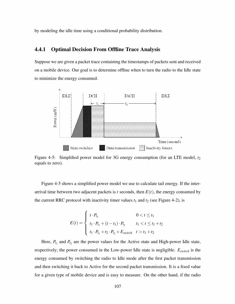
by modeling the idle time using a conditional probability distribution.
4.4.1 Optimal Decision From Offline Trace Analysis
Suppose we are given a packet trace containing the timestamps of packets sent and received
on a mobile device. Our goal is to determine offline when to turn the radio to the Idle state
to minimize the energy consumed.
Figure 4-5: Simplified power model for 3G energy consumption (for an LTE model, t2equals to zero).
Figure 4-5 shows a simplified power model we use to calculate tail energy. If the inter-
arrival time between two adjacent packets is t seconds, then E(t), the energy consumed by
the current RRC protocol with inactivity timer values t1 and t2 (see Figure 4-2), is
E(t) =
t ·Pt1 0 < t ≤ t1
t1 ·Pt1 +(t − t1) ·Pt2 t1 < t ≤ t1 + t2
t1 ·Pt1 + t2 ·Pt2 +Eswitch t > t1 + t2
Here, Pt1 and Pt2 are the power values for the Active state and High-power Idle state,
respectively; the power consumed in the Low-power Idle state is negligible. Eswitch is the
energy consumed by switching the radio to Idle mode after the first packet transmission
and then switching it back to Active for the second packet transmission. It is a fixed value
for a given type of mobile device and is easy to measure. On the other hand, if the radio
107

switches to Idle mode immediately after the first packet transmission finishes, the energy
consumed is just Eswitch.
Figure 4-6: If the energy consumed by the picture on the right is less than the one on theleft, then turning the radio to Idle soon after the first transmission will consume less energythan leaving it on. The energy is easily calculated by integrating the power profiles overtime.
To minimize the energy consumed between packets, the radio should switch to Idle
mode after a packet transmission if, and only if, Eswitch < E(t). Notice that because E(t)
is a monotonically non-decreasing function of t, there exists a value for t, which we call
tthreshold , for which Eswitch < E(t) if and only if t > tthreshold . This expression quantifies
the intuitive idea that after each packet, the radio should switch to Idle mode only if we
know that next packet will not arrive soon: concretely, not arrive in the following tthreshold
seconds. For example, on an HTC Vivid phone in the AT&T 3G network deployed in the
Boston area, tthreshold works out to be 1.2 seconds.
4.4.2 Online Prediction
To minimize energy consumption in practice, we need to predict whether the next packet
will arrive (to be received or to be sent) within tthreshold seconds. Of course, we would like
to make this prediction as quickly as possible, because we would then be able to switch
the radio to Idle mode promptly. We make this prediction by assuming that the packet
inter-arrival distribution observed in the recent past will hold in the near future. After each
packet, the method waits for a short period of time and sees whether any more packets
108

arrive. If a packet arrives, the method resets and waits, but if not, it means a transfer may
be finished and the radio should switch to Idle mode.
The strategy works as follows:
1. Without loss of generality, suppose the current time is t = 0. Compute the conditional
probability that no packet will arrive within twait + tthreshold seconds, given that no
packet has arrived in twait seconds.
P(twait) = P(no packet in twait + tthreshold|no packet in twait)
This conditional distribution is easy to compute given observations of the packet
arrival times of the last several packets.
From the traces we collected, we observed that P(twait) increases as twait increases,
when twait is in the range of [0, tthreshold] (if twait is greater than tthreshold , it means the
radio has been idle for too long a time after the packet transmission, and there is not
much room for energy saving). This property implies that the longer the radio waits
and sees no packet, the higher the likelihood that no packet will arrive soon.
2. Now we need to find twait in order to make the likelihood “high enough”. During
twait , the radio consumes energy, so to decide how much is high enough, we should
take energy consumption into account. Our answer is: P(twait) is high enough if the
expected energy consumption of waiting for twait and then switching states is less
than the expected consumption of waiting for the inactivity timer to time out in the
next twait seconds.
The method determines twait by minimizing the expected energy consumption across
all possible values of twait and taking the value that minimizes the consumption. We
explain how below.
The expected energy consumption of waiting for twait and then switching states is:
E[Ewait_switch] = [Eswitch +E(twait)]
Here, E(twait) is the energy consumed by waiting for twait seconds, and Eswitch is the
109

energy consumed by state switches.
The expected energy consumption of waiting for the inactivity timer to time out is:
E[Eno_switch] =∫ t1+t2
t=0P(inter_arrival_time = t)
dE(t)dt
dt
(4.1)
The following expression now is a function of twait :
f (twait) = E[Eno_switch]−E[Ewait_switch]. (4.2)
The best twait is the one that maximize f (twait), which means that the corresponding
value for twait gives us the highest expected gains over the current RRC protocol.
In implementing this algorithm, we take the latest n packets (we discuss how to choose
n in § 4.6.3) that the control module has seen to construct the inter-arrival distribution. As
new packets are seen, the “window” of the n packet slides forward, and the distribution is
adjusted accordingly.
4.5 MakeActive Algorithm
MakeIdle reduces the 3G wireless energy consumption by switching the radio to Idle mode
frequently. Figure 4-7 (top) shows that MakeIdle may bring more state switches from Idle
to Active and from Active to Idle. These switches cause signaling overhead at the base
station. One idea to reduce the signaling overhead is to “shift” the traffic bursts in order to
combine several traffic bursts together [66, 15], as shown in Figure 4-7(middle and bottom
chart). The longer earlier bursts are delayed, the more bursts we can accumulate, and the
fewer state switches occur.
In this section, we consider only those background applications for which one can de-
lay the traffic for a few seconds without appreciably degrading the user’s experience, not
interactive applications where delaying by a few seconds is unacceptable. Our approach
differs from previous work [66, 15], where the authors aim to reduce energy consumption
110

Figure 4-7: “Shift” traffic to reduce number of state switches.
by batching bursts of traffic together so that they can share the tail energy. By contrast,
because the MakeIdle algorithm already reduces energy by turning the radio to the Idle
mode, MakeActive focuses on reducing the number of state switches to a level comparable
to the status quo. As a result, the amount of delay introduced by this method should be
much smaller than in previous work.
We first consider a relatively straightforward scheme in which the start of a session (i.e.,
a burst of packets) can be delayed by at most a certain maximum delay bound, Tf ix_delay.
We then apply a machine learning algorithm, which induces the same number of state
switches as the fixed delay bound method but in addition reduces the delay for each traffic
burst. Our contribution lies in the application of this algorithm to learn idle durations for
the radio, balancing signaling overhead and increased traffic latency.
111

4.5.1 Fixed Delay Bound
A simple strawman is to set a fixed delay bound, Tf ix_delay. When the radio is in Idle
state, and a socket tries to start a new session at current time t, and no other such requests
are pending, the control module decides to delay turning the radio to Active mode until
t +Tf ix_delay so that other new sessions that might come between time t and t +Tf ix_delay
will all get buffered and will start together at time t+Tf ix_delay. There is a trade-off between
the delay bound and the number of sessions that can be buffered. Note that once a session
begins, its packets do not get further delayed, which means that TCP dynamics should not
be affected by this method.
In the current RRC protocol, the inactivity timers t1 and t2 guarantee that after each
traffic burst, any new burst that comes within t1 + t2 will not introduce extra state switches
between Idle and Active. So in our implementation, we make Tf ix_delay = k × (t1 + t2)
where k is the average number of bursts during each of the radio’s active periods.
4.5.2 Learning Algorithm
The problem with a fixed delay bound is that it does not adapt to the traffic pattern. Every
time the delay is triggered, the first transmission may incur a delay of as long as Tf ix_delay.
We show in the evaluation that a large portion of the traffic bursts get delayed by Tf ix_delay.
However, waiting as long as Tf ix_delay may be overkill; as data accumulates (especially
from different sessions), there comes a point when the radio should switch to Active and
send data before this delay elapses, which will reduce the expected session delay while still
saving energy.
We apply the bank of experts machine learning algorithm [44, 47]. Each “expert” pro-
poses a fixed value for the session delay. In each iteration (each time the radio is in Idle
mode and a transmission occurs), we computed a weighted average value from the experts
and updated the weights according to a loss function. The process to update each expert’s
weight is a standard machine learning process, detailed in the Appendix.
The loss function is a crucial component of the scheme and depends on the details of
the problem to which the learning is applied. Because our goal is to reduce number of state
112

switches by batching, in addition to the delay, the loss function should express the trade-
off between the total time delayed for all the buffered sessions and the number of sessions
buffered. The following equation captures this tradeoff:
L(i) = γDelay(Ti)+1b,γ > 0
Here, γ is a constant scaling parameter between the two parts of the loss function (we
chose 0.008 in our implementation because it gave the best energy-saving results among
the values we tried). Delay(Ti) is the aggregate time delayed over b sessions, if we choose
expert i; b is the number of sessions currently buffered, which is equivalent to the number
of state switches avoided. The 1/b term ensures that as the number of buffered sessions
increases, the value of this part of the loss function reduces, while the other term γDelay(Ti)
may increase.
Let t j be the arrival time of the jth session. Then,
Delay(Ti) =b
∑j=1
Ti − t j.
4.6 Evaluation
We evaluate MakeActive and MakeIdle using trace-driven simulation. We first describe the
simulation setup. Then, we evaluate the two methods using traces collected from popular
applications run by a few real users. Finally, we compare these methods across different
cellular networks.
4.6.1 Simulation Setup
Energy model. One challenge in our simulations is to accurately estimate the energy
consumed given a packet trace containing packet arrival times and packet lengths. Previous
work [34] showed that for 3G/LTE, the value of the energy consumed per bit changes as
the size of traffic bursts changes. Because our methods may change the size of the traffic
bursts (e.g., MakeIdle may decide to switch the radio to Idle mode within a burst), we built
113

our energy model using the energy consumed per second, which is the power for sending
or receiving data.
Network Sending Power (mW) Receiving Power (mW)AT&T 3G 2,043 1,177Verizon LTE 2,928 1,737
Table 4.1: Average power in mW measured on Galaxy Nexus in Verizon network. Theenergy consumed by CPU and screen is subtracted.
Table 4.1 shows the average power consumed when the phone is sending or receiving
bulk data using UDP. Based on this value, we estimate the energy consumed within a traf-
fic burst using the packet inter-arrival time and the packet direction (incoming/outgoing):
For each packet reception, the energy consumed is the inter-arrival time multiplied by the
average receive power, and similarly for each packet transmission.
-0.15
-0.1
-0.05
0
0.05
0.1
0.15
3G LTE
Err
or
Figure 4-8: Simulation energy error for Verizon 3G and LTE networks.
To justify this method, we measured the smartphone’s energy consumption when it was
sending and receiving TCP bulk transfers of different lengths. Each experiment contains
five runs. In each run, the phone sends and receives TCP bulk transfers of three lengths
114

(10 KBytes, 100 KBytes and 1000 KBytes) one after another, with a long-enough idle
period between each transfer. We found that, on average, the error in the estimated energy
consumption is within 10% or less of the true measured value.
One caveat in our energy model is that because fast dormancy is not yet supported on
US 3G/LTE networks when we conducted this measurement, we were unable to accurately
measure the delay to turn the radio from Active to Idle and the energy consumed. We
believe, however, that one can approximate this value by measuring the delay and energy
consumed in turning the data connection off on the phone. In practice, we expect the delay
and energy of fast dormancy switching to be lower, so we model the turn-off energy and
delay for fast dormancy to be 50% of the values measured while turning the radio off. We
also evaluated our methods for reasonable fractions (10%, 20%, 40%) other than 50%, and
found that the results did not change appreciably; hence, we believe that our conclusions
are likely to hold if one were to implement the methods on a device that supports fast
dormancy.
Trace data sets. We collected tcpdump traces on an HTC G1 phone running Android 2.2
for the seven different categories of applications listed below. For each category, we chose
a popular application in the Android market. Each collected trace was 2 hours long. Most
of these applications have the “always on” property in that they usually send or receive data
over the network whenever they run, without necessarily requiring user input.
News: A news reader that has a background process running to fetch breaking news.
Instant Message (IM): An IM application that sends heartbeat packets to the server
periodically, typically every 5 to 20 seconds.
Micro-blog: A micro-blog application, which automatically fetches new tweets without
user input.
Game with ad bar: A game that can run offline but with an advertisement bar that
changes the content roughly once per minute.
Email: This application is run mostly in the background, synchronizing with an email
server every five minutes.
Social Network: A user using the social network application to read the news feeds,
clicks to see pictures, and posts comments. When running in the background, this appli-
115

cation updates only every 30 minutes. We did not collect much background traffic from it.
We used the foreground traffic trace for a comparison trace.
Finance: An application for monitoring the stock market, which updates roughly once
per second when running in the foreground.
We also collected real user data from six different users using Nexus S phones in T-
Mobile’s 3G network and from four different users using Galaxy Nexus phones in Verizon’s
3G/LTE network. All the phones ran tcpdump in the background. Across all users, we
collected 28 days of data. For each user, the amount of data collected varies from two to
five days.
4.6.2 Comparison of Energy Savings
0
20
40
60
80
100
News IM MicroBlog Game Email Social Finance
En
erg
y S
ave
d (
%)
Application
4.5-second95% IATMakeIdleOracleMakeIdle+MakeActive LearnMakeIdle+MakeActive Fix
Figure 4-9: Energy savings for different applications.“4.5-second” sets the inactivity timerto 4.5 seconds. “95% IAT” uses the 95th percentile of packet inter-arrival time observedover the entire trace as the inactivity timer. “MakeIdle” shows the energy saved by ourMakeIdle algorithm. “MakeIdle +MakeActive Learn” and “MakeIdle +MakeActive Fix”show the energy savings when running MakeIdle together with two different MakeActivealgorithms: learning algorithm and fixed delay bound algorithm. Oracle shows the maxi-mum achievable energy savings without delaying any traffic.
116

0
20
40
60
80
100
1 2 3 4 5 6
Energ
y S
aved (
%)
User ID
4.5-second95% IATMakeIdleOracleMakeIdle+MakeActive LearnMakeIdle+MakeActive Fix
(a) Energy savings.
1
2
3
4
5
6
7
1 2 3 4 5 6
Num
ber
of sta
te s
witches
nom
aliz
ed b
y s
tatu
s q
uo
User ID
4.5-second95% IATMakeIdleOracleMakeIdle+MakeActive LearnMakeIdle+MakeActive Fix
(b) Number of state switches normalized by status quo.
0
10
20
30
40
50
60
70
80
1 2 3 4 5 6
Energ
y s
aved p
er
sta
te s
witch (
J)
User ID
4.5-second95% IATMakeIdleOracleMakeIdle+MakeActive LearnMakeIdle+MakeActive Fix
(c) Energy saved per state switch.
Figure 4-10: Energy savings and signaling overhead (number of state switches) across usersin the Verizon 3G network.
117

-20
0
20
40
60
80
100
1 2 3
Energ
y S
aved (
%)
User ID
4.5-second95% IATMakeIdleOracleMakeIdle+MakeActive LearnMakeIdle+MakeActive Fix
(a) Energy savings.
0
10
20
30
40
50
60
1 2 3
Num
ber
of sta
te s
witches
nom
aliz
ed b
y s
tatu
s q
uo
User ID
4.5-second95% IATMakeIdleOracleMakeIdle+MakeActive LearnMakeIdle+MakeActive Fix
(b) Number of state switches normalized by status quo.
0
10
20
30
40
50
60
70
80
90
1 2 3
Energ
y s
aved p
er
sta
te s
witch (
J)
User ID
4.5-second95% IATMakeIdleOracleMakeIdle+MakeActive LearnMakeIdle+MakeActive Fix
(c) Energy saved per state switch.
Figure 4-11: Energy savings and signaling overhead (number of state switches) across usersin the Verizon LTE network.
118

We compared MakeIdle against MakeIdle together with MakeActive (shown as MakeI-
dle+MakeActive) and against two other schemes. The first other scheme is proposed
in [29], in which a trace analysis found that 95% of the packet inter-arrival time values are
smaller than 4.5 seconds. The proposal sets the inactivity timer to a fixed value, t1+t2 = 4.5
seconds. We call this approach “4.5-second tail”.
The second other scheme is that instead of using the value of 4.5 seconds, we drew the
CDF of our traces and got the 95th percentile of packet inter-arrival time observed in each
user’s trace. We call this approach “95% IAT”, which for the data shown in Figure 4-9 hap-
pened to be 1.67 seconds (the value does vary across users and also across applications). In
our evaluation, we are granting this scheme significant leeway because we test the scheme
over the same data on which it has been trained. Despite this advantage, we find that this
scheme has significant limitations.
The “Oracle” is an algorithm in which the packet inter-arrival time is known before the
packet comes, and the algorithm compares the inter-arrival time with the tthreshold defined
in §4.4.1. The Oracle scheme gives us an upper bound of how much energy can be saved
without introducing extra delay. Our MakeIdle + MakeActive algorithm sometimes out-
performs the Oracle because it can delay packets and further reduce the number of state
switches.
Figure 4-9 shows that MakeIdle consistently achieves energy savings close to the Oracle
scheme and outperforms the 4.5-second and 95% IAT schemes. When both MakeIdle and
MakeActive are combined, the savings are greater.
The 95% IAT scheme gives little or negative savings for News and IM, while the other
schemes provide significant positive savings. This is because the 95th percentile value of
the inter-arrival time is highly variable and cannot guarantee savings in all situations. It is
not a robust method.
Figures 4-10a and 4-11a show the estimated energy savings for each user in the Verizon
3G and Verizon LTE networks, respectively. In these results, the different schemes are as
explained above, except that the 95% IAT scheme uses per-user (but not per-application)
inter-arrival time CDFs. The gains of MakeIdle and MakeActive over the other schemes are
substantial in most cases. In the LTE case, the 95% IAT scheme sometimes saves the most
119
energy (for user 2 and user 3), but it sometimes performs worse than MakeIdle (for user 1);
it depends on the user, again showing a lack of robustness. Perhaps more importantly, the
number of state switches is enormous compared to the other schemes, making it extremely
unlikely to be useful in practice.
4.6.3 MakeIdle Evaluation
To understand why MakeIdle outperforms the other methods, we calculated the fraction of
false switches and missed switches for each method. We used Oracle as ground truth and
defined these ratios as follows:
FalseSwitch(FalsePositive) = NFS/(NFS +NT N). Here, NFS is the number of cases in
which the algorithm switches the radio to Idle but Oracle decides to keep the radio in Active
mode. NT N is the number of cases in which both Oracle and the algorithm decide to keep
the radio Active.
MissedSwitch(FalseNegative) = NMS/(NMS +NT P). Here, NMS is the number of cases
where the algorithm decides to keep the radio in the Active mode but Oracle switches the
radio to Idle. NT P is the number of cases where both Oracle and the algorithm switch the
radio to Idle. A high missed switch value means the algorithm tends to keep the radio in
Active mode, which may not be energy efficient.
Figure 4-12 shows these two ratios for different data sets. Note that these values for
MakeIdle are much smaller than for the other two algorithms.
Figure 4-13 shows the false positive and false negative rates (in percentage) as a func-
tion of the number of recent packets used to construct the distribution defined in §4.4.2.
We found that the false negative rate is relatively constant, while the false positive rate
decreases as the window size increases. For all the other results shown in §4.6, we used
n = 100.
Another factor that affects battery consumption is the waiting time between a packet
arrival and the time at which the algorithm actually switches the radio to Idle. For the 4.5-
second tail scheme, the waiting time is always 4.5 seconds. Similarly, the waiting time for
95% IAT is 0.85 seconds for 3G and 0.01 seconds for LTE. In contrast, MakeIdle chooses
120

0
10
20
30
40
50
1 2 3 4 5 6
Fa
lse
Po
sitiv
e o
r F
als
e N
eg
ative
(%
)
User ID
4.5-sec FP4.5-sec FN95% IAT FP95% IAT FNMakeIdle FPMakeIdle FN
(a) Verizon 3G.
0
10
20
30
40
50
1 2 3
Fa
lse
Po
sitiv
e o
r F
als
e N
eg
ative
(%
)
User ID
4.5-sec FP4.5-sec FN95% IAT FP95% IAT FNMakeIdle FPMakeIdle FN
(b) Verizon LTE.
Figure 4-12: False (“FP” short for false positive) and missed switches (“FN” short for falsenegative).
the waiting time dynamically, achieving better gains. Figure 4-14 shows an example of
waiting time changes in a user’s trace in Verizon 3G network.
121

0
0.5
1
1.5
2
2.5
3
3.5
4
4.5
0 50 100 150 200 250 300 350 400
Fa
lse
Po
sitiv
e o
r F
als
e N
eg
ative
(%
)
Window size n
MakeIdle FP
MakeIdle FN
Figure 4-13: False (“FP”) and missed switches (“FN”) changes as the number of packetsused to construct distribution ( defined in § 4.4.2) changes.
0 100 200 300 400 500 6000
0.2
0.4
0.6
0.8
1
1.2
1.4
1.6
Time (seconds)
t wa
it (
se
co
nd
s)
Figure 4-14: Waiting time changes in MakeIdle.
122

4.6.4 MakeActive Evaluation
Although shortening twait with the MakeIdle algorithm saves considerable amounts of en-
ergy, it may bring about more state switches between the Low-power Idle and Active states.
But when there are multiple applications running at the same time, or when one application
starts multiple connections, we can reduce the number of state switches by delaying the
connections and batching them together using MakeActive.
Figures 4-10b and 4-11b show the number of state switches using different algorithms,
normalized by the number measured in the status quo. Each user has several applica-
tions running on the phone. For MakeIdle only, in the 3G/LTE network, the number of
state switches is at most four to five times higher than the status quo. For MakeIdle with
MakeActive, either using the learning algorithm or the fixed-delay bound, the number of
state switches is about the same as the status quo, meaning that by delaying traffic bursts,
our algorithm can reduce the energy consumption without introducing any extra signaling
overhead. Notice that for the 95% IAT algorithm in the LTE network, the number of state
switches is as high as 35× the status quo because the corresponding timer value is only
0.01 seconds. As a result, this method will always switch the radio to Idle even if there
is only a small gap between packets. In a few cases, that does save energy, but at great
expense.
In §4.5, we described both the fixed-delay bound and a learning algorithm. Figure 4-15
shows that using the learning algorithm reduces the average delay for each traffic burst by
50% compared to the fixed-delay bound, while both methods induce a comparable number
of state switches (Figure 4-10b and Figure 4-11b). The learning algorithm is able to reduce
the delay because the loss function (defined in §4.5.2) balances the tradeoff between the
number of buffered bursts and the total delay. Figure 4-16 shows that due to the loss func-
tion, the algorithm will reduce the delay bound as the number of buffered bursts increase.
4.6.5 Different Carriers
To gain a better understanding on how different carriers’ RRC state machine configurations
affect the observed improvement, in this part of the evaluation we ran our trace-driven sim-
123

0
2
4
6
8
10
12
1 2 3 4 5 6
De
lay (
se
co
nd
s)
User ID
Learning meanLearning medianFixed-delay meanFixed-delay median
(a) Verizon 3G network.
0
2
4
6
8
10
12
1 2 3
De
lay (
se
co
nd
s)
User ID
Learning meanLearning medianFixed-delay meanFixed-delay median
(b) Verizon LTE network.
Figure 4-15: Mean and median delays for traffic bursts using learning algorithm and fixeddelay bound scheme.
ulation on different RRC profiles measured from the four major US carriers. In Table 4.2
we list the measured RRC parameters. There are two cases where the inactivity timer t2 = 0
124
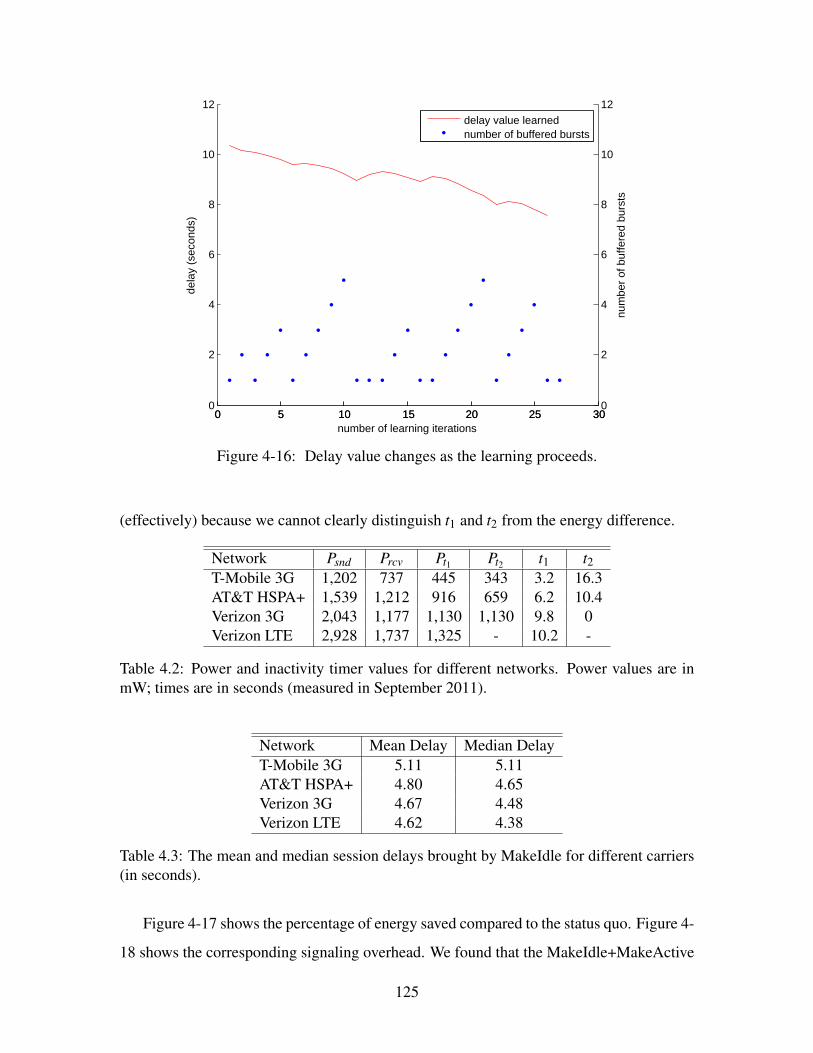
0 5 10 15 20 25 300
2
4
6
8
10
12
number of learning iterations
dela
y (s
econ
ds)
delay value learnednumber of buffered bursts
0 5 10 15 20 25 300
2
4
6
8
10
12
num
ber
of b
uffe
red
burs
ts
Figure 4-16: Delay value changes as the learning proceeds.
(effectively) because we cannot clearly distinguish t1 and t2 from the energy difference.
Network Psnd Prcv Pt1 Pt2 t1 t2T-Mobile 3G 1,202 737 445 343 3.2 16.3AT&T HSPA+ 1,539 1,212 916 659 6.2 10.4Verizon 3G 2,043 1,177 1,130 1,130 9.8 0Verizon LTE 2,928 1,737 1,325 - 10.2 -
Table 4.2: Power and inactivity timer values for different networks. Power values are inmW; times are in seconds (measured in September 2011).
Network Mean Delay Median DelayT-Mobile 3G 5.11 5.11AT&T HSPA+ 4.80 4.65Verizon 3G 4.67 4.48Verizon LTE 4.62 4.38
Table 4.3: The mean and median session delays brought by MakeIdle for different carriers(in seconds).
Figure 4-17 shows the percentage of energy saved compared to the status quo. Figure 4-
18 shows the corresponding signaling overhead. We found that the MakeIdle+MakeActive
125

0
20
40
60
80
100
T-Mobile ATT Verizon3G
VerizonLTE
En
erg
y S
ave
d (
%)
Carriers
4.5-second95% IATMakeIdleOracleMakeIdle+MakeActive LearnMakeIdle+MakeActive Fix
Figure 4-17: Energy saved for different carrier parameters using different methods.For MakeIdle, the maximum gain is 67% in the Verizon LTE network. For MakeI-dle+MakeActive, the maximum gain is 75% achieved in Verizon 3G.
1
2
3
4
5
6
7
8
9
10
11
T-Mobile ATT Verizon3G
VerizonLTE
Nu
mb
er
of
sta
te s
witch
es
no
ma
lize
d b
y s
tatu
s q
uo
Carriers
4.5-second95% IATMakeIdleOracleMakeIdle+MakeActive LearnMakeIdle+MakeActive Fix
Figure 4-18: Number of state switches (signaling overhead) for different methods dividedby number of state switches using the current inactivity timers.
126

method outperforms the 4.5-second tail method in all the carrier settings. Figure 4-18
shows the number of state switches (proportional to signaling overhead) of different schemes
divided by the number of state switches without using any scheme.
The maximum signaling overhead for MakeIdle is less than 3.1× the baseline where
no fast dormancy is triggered. For MakeIdle+MakeActive, the signaling overhead reduces
to only 1.33× or less, a 62% reduction from the previous 3.1×, and is close to the signal-
ing overhead of 4.5-second tail. The session delays brought by MakeActive are listed in
Table 4.3.
In both Figures 4-17 and 4-18, the result shown as MakeIdle has no traffic batching,
which corresponds to the case when all the traffic is treated as delay-sensitive, for example,
web browsing. The MakeActive method is disabled in this case to make sure that the
user’s experience is not adversely affected. One possible method to decide when to disable
MakeActive is for the control module to maintain a list of delay-sensitive or interactive
applications; when any of these applications are running in the foreground, the system
disables MakeActive.
Even without MakeActive, the reduction in energy consumption is still significant in all
four carrier settings. The maximum gain is for Verizon LTE, where MakeIdle saves 67%
energy over the status quo. With MakeIdle, the maximum gain is Verizon 3G, where the
energy saving reaches 75%, and the corresponding median delay is 4.48 seconds.
4.6.6 Energy Overhead of Running Algorithms
To measure the energy overhead of running our methods, we implemented the algorithms
on our test phones. We then generated traffic from the phones based on the user traces we
collected. We ran the traffic generator with and without our methods enabled, ensuring that
it generated the same traffic in all the experiments. We used the power monitor to measure
the total energy consumed in both cases. The energy overhead for running our algorithm is
1.7% for AT&T HTC Vivid and 1.9% for Verizon Galaxy Nexus.
127

0
100
200
300
400
500
600
1 3 5 10 15
Ave
rag
e P
ow
er
(mW
)
Period (sec)
w/o MakeIdlewith MakeIdle
(a) Periodic Ping
0
50
100
150
200
250
300
350
400
Fixed 60 sec Random
Ave
rag
e P
ow
er
(mW
)
w/o MakeIdlewith MakeIdle
(b) Bulk (1 MByte) Download
Figure 4-19: Average power level measured when a Sony Xperia phone was transferringdata with and without MakeIdle enabled.
4.6.7 Implementation Results
Two years after our MakeIdle and MakeActive algorithms were developed, fast dormancy
was enabled in the US and we implemented MakeIdle with the help of our industrial col-
laborator, Foxconn. To achieve better performance, we implemented our algorithm at the
cellular driver layer, a non-open source part of the Android OS. We installed this modified
driver on a Sony Xperia phone connected to AT&T 3G network. We measured the energy
consumption when the phone transferred data with the following traffic patterns:
1. Periodic Ping with various periods,
2. Bulk (1 MByte) downloads with fixed idle interval between each two downloads, and
3. Bulk (1 MByte) downloads with random idle interval.
Figure 4-19 shows the average power level when the phone was transferring data with
different patterns. To calculate the power level, we measured the amount of energy con-
sumed during the transfer, average over the measuring time period. Thus, the energy over-
head of algorithm computation is also included. For comparison, we also measured the
average power level when the phone was loaded with the unmodified driver and was trans-
ferring data with the same traffic pattern. We find that for periodic ping traffic, MakeIdle
can reduce energy consumption by up to 62% (period set to 15 seconds). For bulk down-
load, the energy reductions are 15% for fixed 60-second idle interval and 20% for random
idle interval.
128

4.7 Related Work
We divide related work into measurement studies of 3G energy consumption and approaches
to reduce that energy, 3G usage profiling, and Wi-Fi power saving methods.
4.7.1 3G Energy Mitigation Strategies
Past work aimed at eliminating the tail energy falls into three categories: inactivity timer
reconfiguration, tail cutting, and tail sharing.
Inactivity timer reconfiguration. Lee et al. [40] developed analytic models for energy
consumption in WCDMA and CDMA2000 and showed that the inactivity timer should be
dynamically configured. Falaki et al. [29] proposed an empirical method by plotting the
CDF of packet inter-arrival times for traces collected on smartphones communicating over
3G radio over a long period of time (several days). They found that 95% of the packet
inter-arrival time values are smaller than 4.5 seconds, and proposed setting the inactivity
timer to a fixed value, t1 + t2 = 4.5 seconds. Our approach finds a dynamic inactivity timer
value using traffic pattern information within a short period of time.
Tail cutting. Qian et al. [66] gave an algorithm, TOP, to help the device decide when
to trigger fast dormancy based on the information provided by applications running on
the device. Their algorithm requires the application to predict when the next packet will
come and report it to the OS. This approach requires modifications to the applications,
and it is not clear how each application should make these predictions. Our work requires
no modification to the application code and does not require the application to predict its
traffic.
Traffic batching. Balasubramanian et al. [15] propose an application-layer protocol,
TailEnder, to coalesce separate data transfers by delaying some of them. For delay-tolerant
applications such as email, TailEnder allows applications to set a deadline for the incoming
transfer requests; they suggest and evaluate a relatively long delay of 10 minutes for such
applications. For applications that can benefit from prefetching, TailEnder prefetches 10
web documents for each user query. Their design needs to re-implement the application
and let each application propose its own delay tolerant timers, whereas our design is able
129

to “pause” the traffic transmission at the OS layer.
Liu et al. [41] proposed TailTheft, a traffic queuing and scheduling mechanism to batch
traffic among different applications and share the tail energy among them. One idea of
this work is to set up a timeout value for delay-tolerant transfers and transfer data when
timeouts or other delay-sensitive transfers have triggered the radio to Active mode. Similar
to TailEnder, they require the application to specify how much delay is acceptable.
Another traffic batching approach is prefetching. Qian et al. [65] proposed a prefetching
algorithm for YouTube, which erases the tail between transfers of video pieces.
4.7.2 3G Resource Usage Profiling
Qian et al. [64] designed an algorithm to infer RRC state machine states using packet
traces. The per-application analysis shows that some of the popular mobile applications
have traffic patterns that are not energy-efficient, due to low bit-rate transmission, ineffi-
cient prefetching, and aggressive refresh.
4.7.3 Wi-Fi Power-Saving Algorithms
Much prior work has focused on Wi-Fi power-saving algorithms [38, 39, 69]. The prob-
lem in Wi-Fi networks is qualitatively different from 3G; in Wi-Fi, the time and energy
consumed to transition between states is negligible; what is important is to dynamically
determine the best sleep duration when the Wi-Fi radio is off. In this state, no packets
can be delivered, but the access point will be able to buffer them; the problem is finding
the longest sleep time that ensures that no packets are delayed (say, by a specified max-
imum delay). In the 3G context, changing the state of the radio consumes time, energy,
and network signaling overhead, but there is no risk of receiving packets with excessive
delay because the base station is able to notify a mobile device that packets are waiting
for it even if the device is in Idle state. Thus, we cannot simply apply Wi-Fi power-saving
algorithms to 3G networks. Also, machine learning algorithms have been applied to the
802.11 power saving mode configuration problem [46], but the problem setup is different
for the 3G energy environment because of different tradeoffs we aim to balance.
130

4.7.4 Power-Saving for Processors
Though not directly related to the problem we address, previous work on processor power-
saving has used a similar model to ours in which the different power states and transitions
between different states are abstracted as a state machine [20]. Here, the power-saving
mechanisms are categorized into static methods and adaptive methods, with the adaptive
methods using a nonlinear regression over previous idle/active periods and knowledge of
how successful previous power-saving decisions were.
4.8 Chapter Summary
3G/LTE energy consumption is widely recognized to be a significant problem [15]. We
developed a system to reduce the energy consumption using knowledge of the network
workload. In evaluating the methods on real usage data from nine users over 28 total
days on four different carriers, we find that the energy savings range between 51% and
66% across the carriers for 3G, and is 67% on the Verizon LTE network. When allowing
for delays of a few seconds (acceptable for background applications), the energy savings
increase to between 62% and 75% for 3G, and 71% for LTE. The increased delays reduce
the number of state switches to be the same as in current networks with existing inactivity
timers.
The key idea in this chapter is to adapt the state of the radio to network traffic. To put
the 66% saving (without any delays) or 75% saving (with delay) in perspective, we note
that according to the Nexus 5 specifications, the reduction in lifetime from using the 3G
radio is 10 hours; while it is not clear what application mix produces these numbers, one
might speculate that saving 66% of the energy might correspond to an increase in lifetime
by about 66% of 10 hours, or about 6.6 hours.
131

132

Chapter 5
Conclusion
We conclude the dissertation with a summary of our contributions and discussion of future
work.
5.1 Contributions
This dissertation makes the following contributions:
1. Our measurement study analyzes the wireless network performance of mobile de-
vices in the real world. This measurement study also demonstrates significant poten-
tial improvement if network selection is done properly.
2. The design and implementation of Delphi demonstrated a way to coordinate differ-
ent concerns when making network interface selections. Inside Delphi, we employ
machine learning methods to make network selections. The machine learning mod-
els are trained using network performance data we collected during the measurement
study. As the wireless networks keep advancing, in the future, even the specific pa-
rameters we trained for the current solution, or even the machine learning algorithm,
may not be applicable to make good network selections; however, our modular de-
sign makes sure that the algorithms can be easily replaced. Thus, as long as there
are co-existing networks whose performances are not evenly distributed spatially or
temporally, Delphi’s framework can always be applicable.
3. Both our network selection and energy efficiency solutions require no modification
133

to the application running on the mobile devices. Thus, they can be easily deployed
and improve the performance and user experience of millions of apps already in the
app market.
5.2 Future Work
This dissertation opens up the following directions of future research directions:
Real-world Network Monitoring: As both Wi-Fi and cellular network technologies
keep advancing, it is necessary to keep measuring and monitoring the network performance
for end users. Also, as content distribution networks (CDN) are widely used, mobile de-
vices are more likely to interact with servers that are geographically close to them. Thus,
to reveal the end-to-end network performance, CDN-like measurement server networks
should be deployed.
Network Performance Prediction: As we show in the dissertation, Delphi’s improve-
ment decreases when mobile devices enter new locations. One direction that can be further
explored is to enhance Delphi’s learning capability by using online learning or crowd-
sourced learning mechanisms. This would allow mobile devices to make better network
selection decisions when they enter locations for the first time. Also, applications could
care about other metrics such as average per-packet delay, and tail per-packet delay or
more app-centric metrics such as page-load time for web pages or minimizing the risk of a
stall for streaming video. We view Delphi as a first step in answering these more involved
questions. One direction of our future work is to provide expressive APIs for applications
to express their specific needs to Delphi.
134

Appendix A
Bank of Experts
Here we show how bank of experts [44, 47] works. We bound the maximum delay to n
seconds. Each expert “proposes” a delay value Ti:
Ti = i, i ∈ 1 . . .n.
The output of the algorithm is the weighted average over all the experts:
Tt =n
∑i=1
pt(i)Ti
For each iteration of the updates, the algorithm calculates the probability of each pos-
sible hidden state (in our case, the identity of the expert) based on some observation yt .
Here, we can define the probability of predicting observation yt as P(yt |Ti) = e−L(i,t). The
observation is the number of sessions we batched at time t, and L(i, t) is the loss function.
Then we can apply the following equation to get the weight pt(i):
pt(i) =1Zt
n
∑j=1
pt−1( j)e−L( j,t−1)P(i| j,α).
Here, Zt is a normalization factor that makes sure ∑i pt i = 1. The P(i| j,α) shows the
probability of switching between experts. There are different versions to solve this part.
The one we chose [32] supports switching between the experts and is suitable for cases
135

where the observation may change rapidly, which matches the bursty character of network
traffic. P(i| j,α) is defined as:
P(i| j,α) =
(1−α) i = jα
n−1 i = j
0 ≤ α ≤ 1 is a parameter that determines how quickly the algorithm changes the best
experts. α close to 1 means the network condition changes rapidly and the best expert
always changes. One problem with this algorithm is that it is hard to choose a good α . In
reality, α should not be a fixed value since the network traffic pattern may change rapidly
or remain stationary. We use a more adaptive algorithm, Learn-α [45, 47], to dynamically
choose α .
The basic idea is to first assign m α-experts and use the algorithm above to learn the
proper value of α in each iteration, and then use the up-to-date α to learn Tt [45, 47]. The
final equation for this “two-layer learning” is:
Tt =m
∑j=1
n
∑i=1
p′t( j)pt, j(i)Ti (A.1)
Here, p′t( j) is the weight for the jth α-expert, which is given by:
p′t( j) =1Zt
p′t−1( j)e−L(α j,t−1) (A.2)
This equation shows that p′t( j) is updated from the previous value p′t−1( j); the initial
values are: p′1( j) = 1/m. −L(α j, t −1) is the α loss function, defined as:
L(α j, t) =− logn
∑i=1
pt, j(i)e−L(i,t) (A.3)
Here, L(i, t) is the loss function, discussed in §4.5.2. t is the present time; the loss
function value for the current iteration is calculated from information learned at time t −1.
136

Bibliography
[1] IEEE P802.11ac. Specification Framework for TGac. IEEE 802.11-09/0992r21, 2011.
[2] LTE-Advanced.
[3] 3GPP Release 7: UE Fast Dormancy behavior, 2007. 3GPP discussion and decisionnotes R2-075251.
[4] 3GPP Release 8: 3GPP TS 25.331, 2008.
[5] Data Service Options for Spread Spread Spectrum Systems: Service Options 33 and66, May 2006.
[6] Recognizing the User’s Current Activity. http://developer.android.com/training/location/activity-recognition.html.
[7] AGARWAL, Y., PERING, T., WANT, R., AND GUPTA, R. SwitchR: Reducing Sys-tem Power Consumption in a Multi-Client, Multi-Radio Environment. In WearableComputers (2008).
[8] ios: Using airdrop. http://support.apple.com/kb/HT5887.
[9] Top Sites in United States. http://www.alexa.com/topsites/countries/US.
[10] ANANTHANARAYANAN, G., PADMANABHAN, V. N., RAVINDRANATH, L., AND
THEKKATH, C. A. Combine: Leveraging the Power of Wireless Peers through Col-laborative Downloading. In MobiSys (2007).
[11] ANANTHANARAYANAN, G., AND STOICA, I. Blue-Fi: Enhancing Wi-Fi Perfor-mance Using Bluetooth Signals. In MobiSys (2009).
[12] Android telephony manager api. http://developer.android.com/reference/android/telephony/TelephonyManager.html.
[13] BAHL, P., ADYA, A., PADHYE, J., AND WALMAN, A. Reconsidering WirelessSystems with Multiple Radios. CCR (2004).
[14] BALASUBRAMANIAN, N., BALASUBRAMANIAN, A., AND VENKATARAMANI, A.Energy Consumption in Mobile Phones: A Measurement Study and Implications forNetwork Applications. In IMC (2009).
137

[15] BALASUBRAMANIAN, N., BALASUBRAMANIAN, A., AND VENKATARAMANI, A.Energy Consumption in Mobile Phones: A Measurement Study and Implications forNetwork Applications. In IMC (2009).
[16] BALASUBRAMANIAN, N., BALASUBRAMANIAN, A., AND VENKATARAMANI, A.Energy Consumption in Mobile Phones: a Measurement Study and Implications forNetwork Applications. In IMC (2009).
[17] BARI, F., AND LEUNG, V. Automated Network Selection in a Heterogeneous Wire-less Network Environment. Network, IEEE (2007).
[18] BARLOW-BIGNELL, J., DA SILVA, C., GJENGSET, J., AND OLIHA, P. WirelessInterference and Multipath TCPReducing 3G energy consumption on mobile devices,2013.
[19] BARRÉ, S., PAASCH, C., AND BONAVENTURE, O. Multipath TCP: from Theory toPractice. In NETWORKING 2011. Springer, 2011, pp. 444–457.
[20] BENINI, L., BOGLIOLO, A., AND MICHELI, G. D. A Survey of Design Techniquesfor System-Level Dynamic Power Management. Very Large Scale Integration (VLSI)Systems, IEEE Transactions on (2000).
[21] CARTER, C., KRAVETS, R., AND TOURRILHES, J. Contact Networking: a LocalizedMobility System. In MobiSys (2003).
[22] CHAKRABORTY, A., NAVDA, V., PADMANABHAN, V. N., AND RAMJEE, R. Coor-dinating Cellular Background Transfers Using LoadSense. In MobiCom (2013).
[23] CHANDRA, R., AND BAHL, P. MultiNet: Connecting to Multiple IEEE 802.11 Net-works Using a Single Wireless Card. In INFOCOM (2004).
[24] CHEN, Y.-C., LIM, Y., GIBBENS, R. J., NAHUM, E. M., KHALILI, R., AND
TOWSLEY, D. A Measurement-based Study of Multipath TCP Performance overWireless Networks. In IMC (2013).
[25] DAI, S., TONGAONKAR, A., WANG, X., NUCCI, A., AND SONG, D. Networkpro-filer: Towards Automatic Fingerprinting of Android Apps. In INFOCOM (2013).
[26] DENG, S., AND BALAKRISHNAN, H. Traffic-Aware Techniques to Reduce 3G/LTEWireless Energy Consumption. In CoNEXT (2012).
[27] DENG, S., NETRAVALI, R., SIVARAMAN, A., AND BALAKRISHNAN, H. WiFi,LTE, or Both? Measuring Multi-Homed Wireless Internet Performance. In IMC(2014).
[28] DESHPANDE, P., HOU, X., AND DAS, S. R. Performance Comparison of 3G andMetro-Scale WiFi for Vehicular Network Access. In IMC (2010).
[29] FALAKI, H., LYMBEROPOULOS, D., MAHAJAN, R., KANDULA, S., AND ESTRIN,D. A First Look at Traffic on Smartphones. In IMC (2010).
138

[30] Faster connections, longer-lasting batteries: A fifth of all smartphones now benefitfrom Network Controlled Fast Dormancy. https://blog.networks.nokia.com/mobile-networks/2011/11/28/faster-connections-longer-lasting-batteries-a-fifth-of-all-smartphones-now-benefit-from-network-controlled-fast-dormancy/.
[31] UE "Fast Dormancy" behavior, 2007. 3GPP Discussion and Decision Notes R2-075251.
[32] HERBSTER, M., AND WARMUTH, M. K. Tracking the best expert. Machine Learn-ing 32 (1998), 151–178.
[33] HIGGINS, B. D., REDA, A., ALPEROVICH, T., FLINN, J., GIULI, T. J., NOBLE,B., AND WATSON, D. Intentional Networking: Opportunistic Exploitation of MobileNetwork Diversity. In MobiCom (2010).
[34] HUANG, J., QIAN, F., GERBER, A., MAO, Z. M., SEN, S., AND SPATSCHECK,O. A Close Examination of Performance and Power Characteristics of 4G LTE Net-works. In MobiSys (2012).
[35] JIANG, H., LIU, Z., WANG, Y., LEE, K., AND RHEE, I. Understanding Bufferbloatin Cellular Networks. In CellNet (2012).
[36] KANDULA, S., LIN, K. C.-J., BADIRKHANLI, T., AND KATABI, D. FatVAP: Ag-gregating AP Backhaul Capacity to Maximize Throughput. In NSDI (2008).
[37] KHALILI, R., GAST, N., POPOVIC, M., UPADHYAY, U., AND LE BOUDEC, J.-Y. MPTCP is Not Pareto-Optimal: Performance Issues and a Possible Solution. InCoNEXT (2012).
[38] KRASHINSKY, R., AND BALAKRISHNAN, H. Minimizing Energy for Wireless WebAccess with Bounded Slowdown. In MobiCom (2002).
[39] KRASHINSKY, R., AND BALAKRISHNAN, H. Minimizing Energy for Wireless WebAccess with Bounded Slowdown. ACM Wireless Networks (2005).
[40] LEE, C.-C., YEH, J.-H., AND CHEN, J.-C. Impact of inactivity timer on energyconsumption in WCDMA and CDMA2000. In IEEE Wireless Telecomm. Symp.(WTS)(2004).
[41] LIU, H., ZHANG, Y., AND ZHOU, Y. TailTheft: Leveraging the Wasted Time forSaving Energy in Cellular Communications. In MobiArch (2011).
[42] MAHINDRA, R., VISWANATHAN, H., SUNDARESAN, K., ARSLAN, M. Y., AND
RANGARAJAN, S. A Practical Traffic Management System for Integrated LTE-WiFiNetworks. In MobiCom (2014).
[43] Monsoon power monitor. http://www.msoon.com/LabEquipment/PowerMonitor/.
139

[44] MONTELEONI, C. Online Learning of Non-stationary Sequences. In AI TechnicalReport 2003-011, S.M. Thesis (Artificial Intelligence Laboratory, Massachusetts In-stitute of Technology, 2003).
[45] MONTELEONI, C. Online learning of non-stationary sequences. In AI TechnicalReport 2003-011, S.M. Thesis (Artificial Intelligence Laboratory, Massachusetts In-stitute of Technology, May 2003).
[46] MONTELEONI, C., BALAKRISHNAN, H., FEAMSTER, N., AND JAAKKOLA, T.Managing the 802.11 Energy/Performance Tradeoff with Machine Learning. Tech.Rep. MIT-LCS-TR-971, MIT CSAIL, 2004.
[47] MONTELEONI, C., AND JAAKKOLA, T. Online Learning of Non-stationary Se-quences. In Neural Information Processing Systems 16 (2003).
[48] MPTCP for Android. http://multipath-tcp.org/pmwiki.php/Users/Android.
[49] Apple iOS 7 Surprises as First with New Multipath TCP Connections.http://www.networkworld.com/news/2013/091913-ios7-multipath-273995.html.
[50] Configure MPTCP Routing. http://multipath-tcp.org/pmwiki.php/Users/ConfigureRouting.
[51] MPTCP v0.88 Release. http://multipath-tcp.org/pmwiki.php?n=Main.Release88.
[52] MultiPath TCP - Linux Kernel Implementation. http://www.multipath-tcp.org/.
[53] NETRAVALI, R., SIVARAMAN, A., WINSTEIN, K., DAS, S., GOYAL, A., AND
BALAKRISHNAN, H. Mahimahi: A Lightweight Toolkit for Reproducible Web Mea-surement (Demo). In SIGCOMM (2014).
[54] NIRJON, S., NICOARA, A., HSU, C.-H., SINGH, J., AND STANKOVIC, J. Multi-Nets: Policy Oriented Real-Time Switching of Wireless Interfaces on Mobile De-vices. In RTAS (2012).
[55] NIYATO, D., AND HOSSAIN, E. Dynamics of Network Selection in HeterogeneousWireless Networks: An Evolutionary Game Approach. IEEE Transactions on Vehic-ular Technology (2009).
[56] OLSHEN, L., AND STONE, C. J. Classification and Regression Trees. WadsworthInternational Group (1984).
[57] PAASCH, C., DETAL, G., DUCHENE, F., RAICIU, C., AND BONAVENTURE, O.Exploring Mobile/WiFi Handover with MultiPath TCP. In CellNet (2012).
[58] PAASCH, C., FERLIN, S., ALAY, O., AND BONAVENTURE, O. Experimental Evalu-ation of Multipath TCP Schedulers. In ACM SIGCOMM Capacity Sharing Workshop(CSWS) (2014), ACM.
140

[59] PAREKH, A., AND GALLAGER, R. A Generalized Processor Sharing Approach toFlow Control in Integrated Services Networks: the Single-Node Case. Networking,IEEE/ACM Transactions on (1993).
[60] PEDREGOSA, F., VAROQUAUX, G., GRAMFORT, A., MICHEL, V., THIRION, B.,GRISEL, O., BLONDEL, M., PRETTENHOFER, P., WEISS, R., DUBOURG, V., VAN-DERPLAS, J., PASSOS, A., COURNAPEAU, D., BRUCHER, M., PERROT, M., AND
DUCHESNAY, E. Scikit-learn: Machine learning in Python. Journal of MachineLearning Research (2011).
[61] PERING, T., AGARWAL, Y., GUPTA, R., AND WANT, R. Coolspots: Reducing thePower Consumption of Wireless Mobile Devices with Multiple Radio Interfaces. InMobiSys (2006).
[62] PERKINS, C. E. Mobile IP. Communications Magazine, IEEE (1997).
[63] PLUNTKE, C., EGGERT, L., AND KIUKKONEN, N. Saving Mobile Device Energywith MultiPath TCP. In MobiArch (2011).
[64] QIAN, F., WANG, Z., GERBER, A., MAO, Z., SEN, S., AND SPATSCHECK, O. Pro-filing Resource Usage for Mobile Applications: a Cross-Layer Approach. In MobiSys(2011).
[65] QIAN, F., WANG, Z., GERBER, A., MAO, Z. M., SEN, S., AND SPATSCHECK, O.Characterizing radio resource allocation for 3G networks. In IMC (2010).
[66] QIAN, F., WANG, Z., GERBER, A., MAO, Z. M., SEN, S., AND SPATSCHECK, O.TOP: Tail Optimization Protocol For Celluar Radio Resource Allocation. In ICNP(2010).
[67] RAICIU, C., NICULESCU, D., BAGNULO, M., AND HANDLEY, M. J. OpportunisticMobility with MultiPath TCP. In MobiArch (2011).
[68] ROSEN, S., LEE, S.-J., LEE, J., CONGDON, P., MORLEY MAO, Z., AND BURDEN,K. MCNet: Crowdsourcing Wireless Performance Measurements through the Eyesof Mobile Devices. Communications Magazine, IEEE (2014).
[69] SIMUNIC, T., BENINI, L., GLYNN, P. W., AND MICHELI, G. D. Dynamic powermanagement for portable systems. In MobiCom (2000).
[70] SNOEREN, A. C., AND BALAKRISHNAN, H. An End-to-end Approach to Host Mo-bility. In MobiCom (2000).
[71] SOMMERS, J., AND BARFORD, P. Cell vs. WiFi: on the Performance of Metro AreaMobile Connections. In IMC (2012).
[72] SONG, Q., AND JAMALIPOUR, A. Network Selection in an Integrated Wireless LANand UMTS Environment Using Mathematical Modeling and Computing Techniques.IEEE Wireless Communications (2005).
141

[73] SSL Proxy: Man-in-the-middle. http://crypto.stanford.edu/ssl-mitm/.
[74] Cisco visual networking index: Global mobile data traffic forecast update, 2014-2019. http://www.cisco.com/c/en/us/solutions/collateral/service-provider/visual-networking-index-vni/white_paper_c11-520862.html.
[75] WiFi direct description. http://en.wikipedia.org/wiki/Pearson_product-moment_correlation_coefficient.
[76] WINSTEIN, K., AND BALAKRISHNAN, H. Mosh: An Interactive Remote Shell forMobile Clients. In USENIX ATC (2012).
[77] WISCHIK, D., RAICIU, C., GREENHALGH, A., AND HANDLEY, M. Design, Imple-mentation and Evaluation of Congestion Control for Multipath TCP. In NSDI (2011).
[78] XU, Q., MEHROTRA, S., MAO, Z., AND LI, J. PROTEUS: Network PerformanceForecast for Real-Time, Interactive Mobile Applications. In MobiSys (2013).
[79] YAP, K.-K., HUANG, T.-Y., YIAKOUMIS, Y., CHINCHALI, S., MCKEOWN, N.,AND KATTI, S. Scheduling Packets over Multiple Interfaces While Respecting UserPreferences. In CoNEXT (2013).
[80] YAP, K.-K., MCKEOWN, N., AND KATTI, S. Multi-Server Generalized ProcessorSharing. In ITC (2012).
[81] YEH, J.-H., CHEN, J.-C., AND LEE, C.-C. Comparative Analysis of Energy-SavingTechniques in 3GPP and 3GPP2 Systems. IEEE Trans. on Vehicular Technology(2009).
[82] YEH, J.-H., LEE, C.-C., AND CHEN, J.-C. Performance analysis of energy con-sumption in 3GPP networks. In IEEE Wireless Telecomm. Symp. (WTS) (2004).
[83] Google’s next bid to lower mobile data costs: Zerorating. https://www.theinformation.com/Google-s-Next-Bid-to-Lower-Mobile-Data-Costs-Zero-Rating.
[84] ZHAO, X., CASTELLUCCIA, C., AND BAKER, M. Flexible Network Support forMobility. In MobiCom (1998).
142