Traffic-Aware Techniques to Reduce 3G/LTE WirelessEnergy Consumption

Shuo Deng and Hari BalakrishnanComputer Science and Artificial Intelligence Laboratory

Massachusetts Institute of TechnologyCambridge, MA, USA

shuodeng@csail.mit.edu, hari@csail.mit.edu

ABSTRACTThe 3G/LTE wireless interface is a significant contributor to batterydrain on mobile devices. A large portion of the energy is consumedby unnecessarily keeping the mobile device’s radio in its “Active”mode even when there is no traffic. This paper describes the designof methods to reduce this portion of energy consumption by learningthe traffic patterns and predicting when a burst of traffic will startor end. We develop a technique to determine when to change theradio’s state from Active to Idle, and another to change the radio’sstate from Idle to Active. In evaluating the methods on real usagedata from 9 users over 28 total days on four different carriers, wefind that the energy savings range between 51% and 66% acrossthe carriers for 3G, and is 67% on the Verizon LTE network. Whenallowing for delays of a few seconds (acceptable for backgroundapplications), the energy savings increase to between 62% and 75%for 3G, and 71% for LTE. The increased delays reduce the numberof state switches to be the same as in current networks with existinginactivity timers.

CATEGORIES AND SUBJECT DESCRIPTORSC.2.1 [Computer-Communication Networks]: Network Architec-ture and Design—Wireless communication; C.4 [Performance ofSystems]: Performance attributes; Design studies

GENERAL TERMSDesign, Performance

KEYWORDSCellular Networks, Energy Saving

1. INTRODUCTIONOver a fifth of the 5.5 billion active mobile phones today have

“broadband” data service, and this fraction is rapidly growing. Smart-phones and tablets with wide-area cellular connectivity have becomea significant, and in many cases, dominant, mode of network access.Improvements in the quality of such network connectivity suggestthat mobile Internet access will soon overtake desktop access, es-pecially with the continued proliferation of 3G networks and theemergence of LTE and 4G.

Permission to make digital or hard copies of all or part of this work forpersonal or classroom use is granted without fee provided that copies arenot made or distributed for profit or commercial advantage and that copiesbear this notice and the full citation on the first page. To copy otherwise, torepublish, to post on servers or to redistribute to lists, requires prior specificpermission and/or a fee.CoNEXT’12, December 10–13, 2012, Nice, France.Copyright 2012 ACM 978-1-4503-1775-7/12/12 ...$15.00.

Wide-area cellular wireless protocols need to balance a numberof conflicting goals: high throughput, low latency, low signalingoverhead (signaling is caused by mobility and changes in the mo-bile device’s state), and low battery drain. The 3GPP and 3GPP2standards (used in 3G and LTE) provide some mechanisms for thecellular network operator and the mobile device to optimize thesemetrics [22, 3], but to date, deployed methods to minimize energyconsumption have left a lot to be desired.

The 3G/LTE radio consumes significant amounts of energy; onthe iPhone 4, for example, the stated talk time is “up to 7 hourson 3G” (i.e., when the 3G radio is on and in “typical” use) and“up to 14 hours on 2G”.1 On the Samsung Nexus S, the equivalentnumbers are “up to 6 hours 40 minutes on 3G” and “up to 14 hourson 2G”.2 That the 3G/LTE interface is a battery hog is well-knownto most users anecdotally and from experience, and much advice onthe web and on blogs is available on how to extend the battery lifeof your mobile device.3 Unfortunately, essentially all such advicesays to “disable your 3G data radio” and “change your fetch datasettings to reduce network usage”. Such advice largely defeats thepurpose of having an “always on” broadband-speed wireless device,but appears to be the best one can do in current deployments.

We show the measured values of 3G energy consumption formultiple Android applications in Figure 1.4 This bar graph showsthe percentage of energy consumed by different 3G radio states. Formost of these applications (which are all background applicationsthat can generate traffic without user input, except for Facebook),less than 30% of the energy consumed was during the actual trans-mission or reception of data. Previous research arrived at a similarconclusion [4]: about 60% of the energy consumed by the 3G inter-face is spent when the radio is not transmitting or receiving data.

In principle, one might imagine that simply turning the radio offor switching it to a low-power idle state is all it takes to reduceenergy consumption. This approach does not work for three reasons.First, switching between the active and the different idle states takesa few seconds because it involves communication with the basestation, so it should be done only if there is good reason to believethat making the transition is useful for a reasonable duration of timein the future. Second, switching states consumes energy, whichmeans that if done without care, overall energy consumption willincrease compared to not doing anything at all. Third, the switchingincurs signaling overhead on the wireless network, which means

1http://www.apple.com/iphone/specs.html2http://www.gsmarena.com/samsung_google_nexus_s-3620.php3http://www.intomobile.com/2008/07/23/extend-your-iphone-3gs-battery-life/4An HTC G1 phone connected to a power monitor [13], with onlyone application running, at one indoor location.

Figure 1: Energy consumed by the 3G interface. “Data” cor-responds to a data transmission; “DCH Timer” and “FACHTimer” are each the energy consumed with the radio in the idlestates specified by the two timers, and “State Switch” is theenergy consumed in switching states. These timers and stateswitches are described in §2.

that it should be done only if the benefits are substantial relative tothe cost on the network.

This paper tackles these challenges and develops a solution toreduce 3G/LTE energy consumption without appreciably degradingapplication performance or introducing a significant amount of sig-naling overhead on the network. Unlike currently deployed methodsthat simply switch between radio states after fixed time intervals—an approach known to be rather crude and sub-optimal [21, 4, 11,19])– our approach is to observe network traffic activity on the mo-bile device and switch between the different radio states by adaptingto the workload.

The key idea is that by observing network traffic activity, a controlmodule on the mobile device can adapt the 3G/LTE radio statetransitions to the workload. We apply statistical machine learningtechniques to predict network activity and make transitions that aresuggested by the statistical models. This approach is well-suited tothe emerging fast dormancy mechanism [1, 2] that allows a radio torapidly move between the Active and Idle states and vice versa. Ourgoal is to reduce the energy consumed by networked backgroundapplications on mobile devices.

This paper makes the following contributions:1. A traffic-aware design to control the state transitions of a 3G/LTE

radio taking energy consumption, latency, and signaling overheadinto consideration. The design incorporates two algorithms:

(a) MakeIdle, which uses aggregate traffic activity to predict theend of an active session by building a conditional probabilitydistribution of network activity.

(b) MakeActive, which delays the start of a new session by afew seconds to allow multiple sessions to all become activeat the same time and therefore reduce signaling overhead.This method is appropriate for non-interactive backgroundapplications that can tolerate some delay.

2. An experimental evaluation of these methods on real usage datafrom nine users over 28 total days on four different carriers. Wefind that the energy savings compared to the status quo rangebetween 51% and 66% across the carriers for 3G, and is 67%on the Verizon LTE network. When allowing for delays of afew seconds (acceptable for background applications), the energysavings increase to between 62% and 75% for 3G, and 71% for

(a) 3G RRC.

(b) LTE RRC.

Figure 2: Radio Resource Control (RRC) State Machine.

LTE. The increased delays reduce the number of state switches tobe the same as in current networks with existing inactivity timers.

2. BACKGROUNDThis section describes the 3G/LTE state machine and its energy

consumption.

2.1 3G/LTE State MachineThe Radio Resource Control (RRC) protocol, which is part of the

3GPP standard, incorporates the state machine for energy manage-ment shown in Figure 2.

The base station maintains two inactivity timers, t1 and t2, foreach mobile device. For a device maintaining a dedicated channelin the Active (Cell_DCH) state with the base station, if the basestation sees no data activity to or from the device for t1 seconds,it will switch the device from the dedicated channel to a sharedlow-speed channel, transitioning the device to the “High-power idle”(Cell_FACH) state. This state consumes less power than “Active”,but still consumes a non-negligible amount of power. If there isno further data activity between the device and base station foranother t2 seconds, the base station will turn the device to either theCell_PCH or IDLE state. We refer to the Cell_PCH and IDLE statestogether as the “Idle” state, because the device consumes essentiallyno power in either state. For LTE networks (Figure 2(b)), there areonly two states: RRC_CONNECTED and RRC_IDLE (there aresubstates in RRC_CONNECTED [8], which we do not discuss herebecause they are not relevant), and one inactivity timer, shown as t1.

The inactivity timers (t1 and t2) are useful because a state transi-tion from “Idle” to “Active” (Cell_DCH) incurs significant delays.For example, in our measurements in the Boston area, these valuesare ≈ 1.4 seconds on AT&T’s 3G network, ≈ 3.6 seconds on T-Mobile’s 3G network, ≈ 2.0 seconds on Sprint’s 3G network, ≈ 1.0second on Sprint’s LTE network, ≈ 1.2 seconds on Verizon’s 3Gnetwork, and ≈ 0.6 seconds on Verizon’s LTE network (these num-bers may vary across different regions). Each state transition alsoconsumes energy on the device and incurs signaling overhead for

the base station to allocate a dedicated channel to the device. Theinactivity timers also prevent the base station from frequently releas-ing and re-allocating channels to devices which causes per-packetdelay for the device to be high.

The description given above captures the salient features of the3GPP standard. Another popular 3G standard is 3GPP2 [3]. Al-though 3GPP2 networks use different techniques, from the per-spective of energy consumption, they are essentially identical to3GPP [21]; like 3GPP, 3GPP2 networks also have different powerlevels for different states on the device side, and use similar inactiv-ity timers for state transitions. For concreteness, in this paper, wefocus on 3GPP networks.

2.2 Energy ConsumptionWe measured the power consumption and inactivity timer values

using the Monsoon Power Monitor [13]. Figure 3 shows graphsof our measurements during a radio state switches cycle on anHTC Vivid smartphone in AT&T’s 3G network and on a GalaxyNexus smartphone in Verizon’s LTE network. (We show results forother carriers in Section 6.) During the High-power idle (FACH forAT&T) and part of Active (DCH for AT&T, RRC_CONNECTEDfor Verizon) states, there is no data transmission. The RRC statemachine keeps the radio on here in case a new transmission or re-ception occurs in the near future. Consistent with previous work [4],we use the term tail to refer to this duration when the radio is on butthere is no data transmission.

We measured the inactivity timer values in AT&T’s 3G networkin the Boston area to be t1 ≈ 6.2 seconds and t2 ≈ 10.4 seconds. Theenergy consumed at the end of a data transfer when the radio is inone of the two Idle states before turning off is termed the tail energy;this energy can be 60% or more of the total energy consumption of3G [4].

3GPP Release 7 [1] proposed a feature called fast dormancy,which allows the device to actively release the channel by itselfbefore the inactivity timer times out on the base station. One of theissues that then arises is that the base station loses control over theconnection when mobile devices are able to disconnect by them-selves. In 3GPP Release 8 [2], fast dormancy was changed: themobile device first sends a fast dormancy request, and the basestation will decide to release the channel or not. In Europe, NokiaSiemens Networks has applied Network Controlled Fast Dormancybased on 3GPP Release 8. Because it is not entirely clear whatpolicy any given network carrier will use to decide whether to re-lease the channel upon receiving a request at a base station, in oursimplified model, we assume that if the base station is running 3GPPRelease 8, whenever the phone sends a fast dormancy request tothe base station, the base station will accept and release the channel.Our goal is to evaluate the network signaling overhead of such astrategy as a way to help inform network-carrier policy.

3. DESIGNThe key insight in our approach to reduce 3G energy consumption

is that by observing and adapting to network activity, a controlmodule can predict when to put the radio into its Idle state, andwhen to move from Idle to Active state. These state transitions takea non-trivial amount of time—between 1 and 3 seconds—and alsoadd signaling overhead because each transition is accompanied by afew messages between the device and the base station. Hence, theintuition in our approach is to predict the occurrence of bursts ofnetwork activity, so that the control module can put the radio intothe idle mode when it believes a burst has ended, which means therewill not be any more traffic in the future for a relatively long periodof time. Conversely, the idea is to put the radio in active mode when“enough” bursts of traffic accumulate.

(a) HTC Vivid in AT&T 3G Network.

(b) Galaxy Nexus in Verizon LTE Network.

Figure 3: The measured power consumption of the differentRRC states. Exact values can be found in Table 2. In these fig-ures the power level for IDLE/RRC_IDLE is non-zero becauseof the CPU and LED screen power consumption.

To achieve the prediction, our approach needs to observe networkactivity and be able to pause data transmissions. To make ourapproach work with existing applications, we should not require anychange to the application code. To achieve these goals, we modifiedthe socket layer and added a control module inside the Android OSsource code.

Our system has two software modules: one that modifies thelibrary used by applications to communicate with the socket layer,and another that implements the control module, as shown in Fig-ure 4. The first module informs the control module of all socketcalls; in response, the control module configures the state of theradio. The fast dormancy interface is shown as a dashed modulebecause our system uses it if it is available.

The control module implements two different methods. The firstmethod, called MakeIdle, runs when the radio is in the Active state(Cell_DCH or RRC_CONNECTED) and determines when the radioshould be put into the Idle (IDLE or Cell_PCH or RRC_IDLE) state.The second method, called MakeActive, runs when the radio is inthe Idle state. In this state, it cannot send any packets without firstmoving to the Active state; MakeActive determines how long theradio should be idle before moving to active state.

Figure 4: System design.

Figure 5: Simplified power model for 3G energy consumption(for an LTE model, t2 equals to zero).

4. MAKEIDLE ALGORITHMInstead of using a fixed inactivity timer, the MakeIdle method

dynamically decides when to put the radio into Idle mode aftereach packet transmission or reception. We first show in §4.1 howto compute the optimal decision given complete knowledge of apacket trace: the result is that the radio should be turned to Idleif there is a gap of more than a certain threshold amount of timein the trace, which depends on measurable parameters. Then, in§4.2, we develop an online method to predict idle durations that willexceed this threshold by modeling the idle time using a conditionalprobability distribution.

4.1 Optimal Decision From Offline Trace AnalysisSuppose we are given a packet trace containing the timestamps

of packets sent and received on a mobile device. Our goal is todetermine offline when to turn the radio to the Idle state to minimizethe energy consumed.

Figure 5 shows a simplified power model we use to calculatetail energy. If the inter-arrival time between two adjacent packetsis t seconds, then E(t), the energy consumed by the current RRCprotocol with inactivity timer values t1 and t2 (see Figure 2), is

E(t) =

t ·Pt1 0 < t ≤ t1t1 ·Pt1 +(t− t1) ·Pt2 t1 < t ≤ t1 + t2t1 ·Pt1 + t2 ·Pt2 +Eswitch t > t1 + t2

Here, Pt1 and Pt2 are the power values for the active state and high-power idle state, respectively; the power consumed in the low-poweridle state is negligible. Eswitch is the energy consumed by switchingthe radio to Idle mode after the first packet transmission and thenswitching it back to Active for the second packet transmission. It

Figure 6: If the energy consumed by the picture on the rightis less than the one on the left, then turning the radio to Idlesoon after the first transmission will consume less energy thanleaving it on. The energy is easily calculated by integrating thepower profiles over time.

is a fixed value for a given type of mobile device and is easy tomeasure.

On the other hand, if the radio switches to Idle mode immediatelyafter the first packet transmission finishes, the energy consumed isjust Eswitch.

To minimize the energy consumed between packets, the radioshould switch to Idle mode after a packet transmission if, and onlyif, Eswitch < E(t). Notice that because E(t) is a monotonically non-decreasing function of t, there exists a value for t, which we calltthreshold , for which Eswitch < E(t) if and only if t > tthreshold . Thisexpression quantifies the intuitive idea that after each packet, theradio should switch to Idle mode only if we know that next packetwill not arrive soon; concretely, not arrive in the following tthresholdseconds. For example, on an HTC Vivid phone in the AT&T 3Gnetwork deployed in the Boston area, tthreshold works out to be 1.2seconds.

4.2 Online PredictionTo minimize energy consumption in practice, we need to predict

whether the next packet will arrive (to be received or to be sent)within tthreshold seconds. Of course, we would like to make thisprediction as quickly as possible, because we would then be able toswitch the radio to Idle mode promptly. We make this predictionby assuming that the packet inter-arrival distribution observed inthe recent past will hold in the near future. After each packet, themethod waits for a short period of time and sees whether any morepackets arrive. If a packet arrives, the method resets and waits, but ifnot, it means a transfer may be finished and the radio should switchto Idle mode.

The strategy works as follows:1. Without loss of generality, suppose the current time is t = 0.

Compute the conditional probability that no packet will arrivewithin twait + tthreshold seconds, given that no packet has arrivedin twait seconds.

P(twait) = P(no packet in twait + tthreshold |no packet in twait)

This conditional distribution is easy to compute given observa-tions of the packet arrival times of the last several packets.From the traces we collected, we observed that P(twait) increasesas twait increases, when twait is in the range of [0, tthreshold ] (iftwait is greater than tthreshold , it means the radio has been idle fortoo long time after the packet transmission and there is not muchroom for energy saving). This property implies that the longerthe radio waits and sees no packet, the higher the likelihood thatno packet will arrive soon.

2. Now we need to find twait in order to make the likelihood “highenough”. During twait , the radio consumes energy, so to decidehow much is “high enough”, we should take energy consump-

tion into account. Our answer is: P(twait) is “high enough” ifthe expected energy consumption of waiting for twait and thenswitching states is less than the expected consumption of waitingfor the inactivity timer to time out in the next twait seconds.The method determines twait by minimizing the expected energyconsumption across all possible values of twait , and taking thevalue that minimizes the consumption. We explain how below.

The expected energy consumption of waiting for twait and thenswitching states is:

E[Ewait_switch] = [Eswitch +E(twait)]

Here, E(twait) is the energy consumed by waiting for twait secondsand Eswitch is the energy consumed by state switches.

The expected energy consumption of waiting for inactivity timerto time out is:

E[Eno_switch] =∫ t1+t2

t=0P(inter_arrival_time = t)

dE(t)dt

dt

(1)

The following expression now is a function of twait :

f (twait) = E[Eno_switch]−E[Ewait_switch]. (2)

The best twait is the one that maximize f (twait), which means thatthe corresponding value for twait gives us highest expected gainsover the current RRC protocol.

In implementing this algorithm, we take the latest n packets (wediscuss how to choose n in Section 6.3) that the control modulehas seen, to construct the inter-arrival distribution. As new packetsare seen, the “window” of the n packet slides forward, and thedistribution is adjusted accordingly.

5. MAKEACTIVE ALGORITHM

Figure 7: “Shift” traffic to reduce number of state switches.

MakeIdle reduces the 3G wireless energy consumption by switch-ing the radio to Idle mode frequently. Figure 7 (top) shows thatMakeIdle may bring more state switches from Idle to Active andfrom Active to Idle. These switches cause signaling overhead atthe base station. One idea to reduce the signaling overhead is to“shift” the traffic bursts in order to combine several traffic burststogether [19, 4], as shown in Figure 7(middle and bottom chart). Thelonger earlier bursts are delayed, the more bursts we can accumulateand the fewer state switches occur.

In this section, we only consider those background applicationsfor which one can delay the traffic for a few seconds without appre-ciably degrading the user’s experience, not interactive applicationswhere delaying by a few seconds is unacceptable. Our approachdiffers from previous work [19, 4], where the authors aim to reduceenergy consumption by batching bursts of traffic together so thatthey can share the tail energy. By contrast, because the MakeIdlealgorithm already reduces energy by turn radio to the idle mode,MakeActive focuses on reducing the number of state switches to alevel comparable to the status quo. As a result, the amount of delayintroduced by this method should be much smaller than in previouswork.

We first consider a relatively straightforward scheme in whichthe start of a session (i.e., a burst of packets) can be delayed by atmost a certain maximum delay bound, Tf ix_delay. We then applya machine learning algorithm, which induces the same number ofstate switches as the fixed delay bound method, but in additionreduces the delay for each traffic burst. Our contribution lies in theapplication of this algorithm to learn idle durations for the radio,balancing signaling overhead and increased traffic latency.

5.1 Fixed Delay BoundA simple strawman is to set a fixed delay bound, Tf ix_delay. When

the radio is in Idle state and a socket tries to start a new session atcurrent time t, and no other such requests are pending, the controlmodule decides to delay turning the radio to Active mode untilt +Tf ix_delay, so that other new sessions that might come betweentime t and t +Tf ix_delay will all get buffered and will start togetherat time t +Tf ix_delay. There is a trade-off between the delay boundand the number of sessions that can be buffered. Note that once asession begins, its packets do not get further delayed, which meansthat TCP dynamics should not be affected by this method.

In the current RRC protocol, the inactivity timers t1 and t2 guar-antee that after each traffic burst, any new burst comes within t1 + t2will not introduce extra state switches between Idle and Active. Soin our implementation, we make Tf ix_delay = k× (t1 + t2) where kis the average number of bursts during each of the radio’s activeperiod.

5.2 Learning AlgorithmThe problem with a fixed delay bound is that it does not adapt

to the traffic pattern. Every time the delay is triggered, the firsttransmission may incur a delay of as long as Tf ix_delay. We show inthe evaluation that a large portion of the traffic bursts get delayed byTf ix_delay. However, waiting as long as Tf ix_delay may be overkill; asdata accumulates (especially from different sessions), there comes apoint when the radio should switch to Active and data sent beforethis delay elapses, which will reduce the expected session delaywhile still saving energy.

We apply the bank of experts machine learning algorithm [14, 16].Each “expert” proposes a fixed value for the session delay. In eachiteration (each time the radio is in Idle mode and a transmissionoccurs), we computed a weighted average value from the expertsand update the weights according to a loss function. The process toupdate each expert’s weight is a standard machine learning process,detailed in the appendix.

The loss function is a crucial component of the scheme and de-pends on the details of the problem to which the learning is applied.Because our goal is to reduce number of state switches by batching,in addition to the delay, the loss function should express the trade-offbetween the total time delayed for all the buffered sessions and thenumber of session buffered. The following equation captures thistradeoff:

L(i) = γDelay(Ti)+1b,γ > 0

Here, γ is a constant scaling parameter between the two parts ofthe loss function (we chose 0.008 in our implementation becauseit gave the best energy-saving results among the values we tried).Delay(Ti) is the aggregate time delayed over b sessions, if we chooseexpert i. b is the number of sessions currently buffered, whichis equivalent to the number of state switches avoided. The 1/bterm ensures that as the number of buffered sessions increases, thevalue of this part of the loss function reduces, while the other termγDelay(Ti) may increase.

Let t j be the arrival time of the jth session. Then,

Delay(Ti) =b

∑j=1

Ti− t j.

6. EVALUATIONWe evaluate MakeActive and MakeIdle using trace-driven sim-

ulation. We first describe the simulation setup. Then, we evaluatethe two methods using traces collected from popular applicationsrun by a few real users. Finally, we compare these methods acrossdifferent cellular networks.

6.1 Simulation SetupEnergy model. One challenge in our simulations is to accuratelyestimate the energy consumed given a packet trace containing packetarrival times and packet lengths. Previous work [8] showed that for3G/LTE, the value of the energy consumed per bit changes as thesize of traffic bursts changes. Because our methods may change thesize of the traffic bursts, (e.g., MakeIdle may decide to switch theradio to Idle mode within a burst), we build our energy model usingthe energy consumed per second, which is the power for sending orreceiving data.

Network Sending Power (mW) Receiving Power (mW)AT&T 3G 2043 1177Verizon LTE 2928 1737

Table 1: Average power in mW measured on Galaxy Nexus inVerizon Network. The energy consumed by CPU and screen issubtracted.

Table 1 shows the average power consumed when the phone issending or receiving bulk data using UDP. Based on this value, weestimate the energy consumed within a traffic burst using the packetinter-arrival time and the packet direction (incoming/outgoing): foreach packet reception, the energy consumed is the inter-arrival timemultiplied by the average receive power, and similarly for eachpacket transmission.

To justify this method, we measure the smartphone’s energyconsumption when it is sending and receiving TCP bulk transfers ofdifferent lengths. Each experiment contains five runs. In each run,the phone sends and receives TCP bulk transfers of three lengths(10 kBytes, 100 kBytes and 1000 kBytes) one after another, witha long-enough idle period between each transfer. We find that, onaverage, the error in the estimated energy consumption is within10% or less of the true measured value.

One caveat in our energy model is that because fast dormancyis not yet supported on US 3G/LTE networks, we were unableto accurately measure the delay to turn the radio from Active toIdle and the energy consumed. We believe, however, that one can

-0.15

-0.1

-0.05

0

0.05

0.1

0.15

3G LTE

Err

or

Figure 8: Simulation energy error for Verizon 3G and LTE net-works.

approximate this value by measuring the delay and energy consumedin turning the data connection off on the phone. In practice, weexpect the delay and energy of fast dormancy switching to be lower,so we model the turn-off energy and delay for fast dormancy tobe 50% of the values measured while turning the radio off. Wealso evaluated our methods for reasonable fractions (10%, 20%,40%) other than 50%, and found that the results did not changeappreciably; hence, we believe that our conclusions are likely tohold if one were to implement the methods on a device that supportsfast dormancy.

Trace data sets. We collected tcpdump traces on an HTC G1phone running Android 2.2 for the seven different categories ofapplications listed below. For each category, we choose a popularapplication in the Android Market. Each collected trace was 2 hourslong. Most of these applications have the “always on” property inthat they usually send or receive data over the network wheneverthey run, without necessarily requiring user input.

News: A news reader that has a background process running tofetch breaking news.

Instant Message (IM): An IM application that sends heartbeatpackets to the server periodically, typically every 5 to 20 seconds.

Micro-blog: A micro-blog application, which automaticallyfetches new tweets without user input.

Game with ad bar: A game that can run offline, but with anadvertisement bar that changes the content roughly once per minute.

Email: This application is run mostly in the background, synchro-nizing with an email server every five minutes.

Social Network: A user using the social network application toread the news feeds, clicks to see pictures, and posts comments.When running in background, this application updates only every30 minutes. We did not collect much background traffic from it. Weuse the foreground traffic trace for comparison trace.

Finance: An application for monitoring the stock market, whichupdates roughly once per second when running in the foreground.

We also collected real user data from six different users usingNexus S phones in T-Mobile’s 3G network and from four differentusers using Galaxy Nexus phones in Verizon’s 3G/LTE network.All the phones run tcpdump in the background. Across all users,we collected 28 days of data. For each user, the amount of datacollected varies from two to five days.

6.2 Comparison of Energy Savings

0

20

40

60

80

100

News IM MicroBlog Game Email Social Finance

En

erg

y S

ave

d (

%)

Application

4.5-second95% IATMakeIdleOracleMakeIdle+MakeActive LearnMakeIdle+MakeActive Fix

Figure 9: Energy savings for different applications.“4.5-second” sets the inactivity timer to 4.5 seconds. “95% IAT”uses the 95th percentile of packet inter-arrival time observedover the entire trace as the inactivity timer. “MakeIdle” showsthe energy saved by our MakeIdle algorithm. “MakeIdle+MakeActive Learn” and “MakeIdle +MakeActive Fix” showthe energy savings when running MakeIdle together with twodifferent MakeActive algorithms: learning algorithm and fixeddelay bound algorithm. Oracle shows the maximum achievableenergy savings without delaying any traffic.

We compare MakeIdle against MakeIdle together with Make-Active (shown as MakeIdle+MakeActive), and against two otherschemes. The first other scheme is proposed in [6], where a traceanalysis found that 95% of the packet inter-arrival time values aresmaller than 4.5 seconds. The proposal sets the inactivity timer to afixed value, t1+t2 = 4.5 seconds. We call this approach “4.5-secondtail”.

The second other scheme is that instead of using the value of 4.5seconds, we draw the CDF of our traces and get the 95th percentileof packet inter-arrival time observed in each user’s trace. We callthis approach “95% IAT”, which for the data shown in Figure 9 cor-responding to one user happened to be 1.67 seconds (the value doesvary across users and also across applications). In our evaluation,we are granting this scheme significant leeway because we test thescheme over the same data on which it has been trained. Despitethis advantage, we find that this scheme has significant limitations.

The “Oracle” is an algorithm in which the packet inter-arrivaltime is known before packet comes, and the algorithm comparesthe inter-arrival time with the tthreshold defined in Section 4.1. TheOracle scheme gives us an upper bound of how much energy can besaved without introducing extra delay. Our MakeIdle + MakeActivealgorithm sometimes outperforms the Oracle because it can delaypackets and further reduce the number of state switches.

Figure 9 shows that MakeIdle consistently achieves energy sav-ings close to the Oracle scheme, and outperforms the “4.5-second”and “95%” IAT schemes. When both MakeIdle and MakeActive arecombined, the savings are greater.

The “95% IAT” scheme gives little or negative savings for “News”and “IM”, while the other schemes provide significant positivesavings. This is because the 95% percentile of the inter-arrival timeis highly variable and cannot guarantee savings in all situations. Itis not a robust method.

Figures 10(a) and 11(a) show the estimated energy savings foreach user in the Verizon 3G and Verizon LTE networks, respectively.

In these results, the different schemes are as explained above, exceptthat the 95% IAT scheme uses per-user (but not per-application)inter-arrival time CDFs. The gains of MakeIdle and MakeActiveover the other schemes are substantial in most cases. In the LTEcase, the 95% IAT scheme sometimes saves the most energy (foruser 2 and user 3), but sometimes performs worse than MakeIdle (foruser 1); it depends on the user, again showing a lack of robustness.Perhaps more importantly, the number of state switches is enormouscompared to the other schemes, making it extremely unlikely to beuseful in practice.

6.3 MakeIdle Evaluation

0

10

20

30

40

50

1 2 3 4 5 6

Fa

lse

Po

sitiv

e o

r F

als

e N

eg

ative

(%

)

User ID

4.5-sec FP4.5-sec FN95% IAT FP95% IAT FNMakeIdle FPMakeIdle FN

(a) Verizon 3G.

0

10

20

30

40

50

1 2 3

Fa

lse

Po

sitiv

e o

r F

als

e N

eg

ative

(%

)

User ID

4.5-sec FP4.5-sec FN95% IAT FP95% IAT FNMakeIdle FPMakeIdle FN

(b) Verizon LTE.

Figure 12: False (“FP” short for false positive) and missedswitches (“FN” short for false negative).

To understand why MakeIdle outperforms the other methods, wecalculate the fraction of false switches and missed switches for eachmethod. We use “Oracle” as ground truth and define these ratios asfollows:

FalseSwitch(FalsePositive) = NFS/(NFS +NT N). Here, NFS isthe number of cases where the algorithm switches the radio to Idlebut Oracle decides to keep the radio in Active mode. NT N is thenumber of cases where both Oracle and the algorithm decide to keepthe radio Active.

MissedSwitch(FalseNegative) = NMS/(NMS+NT P). Here, NMSis the number of cases where the algorithm decides to keep the radioin the Active mode but Oracle switches the radio to Idle. NT P is thenumber of cases where both Oracle and the algorithm switch theradio to Idle. A high missed switch value means the algorithm tendsto keep the radio in Active mode, which may not be energy-efficient.

Figure 12 shows these two ratios for different data sets. Note thatthese values for MakeIdle are much smaller than for the other twoalgorithms.

Figure 13 shows the false positive and false negative rates (inpercentage) as a function of the number of recent packets used toconstruct the distribution defined in Section 4.2. We find that thefalse negative rate is relatively constant, while the false positive ratedecreases as the window size increases. For all the other resultsshown in §6, we use n = 100.

Another factor that affects battery consumption is the waitingtime between a packet arrival and the time at which the algorithmactually switches the radio to Idle. For the “4.5-second tail” scheme,the waiting time is always 4.5 seconds. Similarly, the waiting timefor “95% IAT” is 0.85 seconds for 3G and 0.01 seconds for LTE. Incontrast, MakeIdle chooses the waiting time dynamically, achievingbetter gains. Figure 14 shows an example of waiting time changesin a user’s trace in Verizon 3G network.

6.4 MakeActive EvaluationAlthough shortening twait with the MakeIdle algorithm saves

considerable amounts of energy, it may bring about more stateswitches between the Low-power idle and Active states. But whenthere are multiple applications running at the same time, or when one

0

20

40

60

80

100

1 2 3 4 5 6

Energ

y S

aved (

%)

User ID

4.5-second95% IATMakeIdleOracleMakeIdle+MakeActive LearnMakeIdle+MakeActive Fix

(a) Energy savings.

1

2

3

4

5

6

7

1 2 3 4 5 6

Num

ber

of sta

te s

witches

nom

aliz

ed b

y s

tatu

s q

uo

User ID

4.5-second95% IATMakeIdleOracleMakeIdle+MakeActive LearnMakeIdle+MakeActive Fix

(b) Number of state switches normalized bystatus quo.

0

10

20

30

40

50

60

70

80

1 2 3 4 5 6

Energ

y s

aved p

er

sta

te s

witch (

J)

User ID

4.5-second95% IATMakeIdleOracleMakeIdle+MakeActive LearnMakeIdle+MakeActive Fix

(c) Energy saved per state switch.

Figure 10: Energy savings and signaling overhead (number of state switches) across users in the Verizon 3G network.

-20

0

20

40

60

80

100

1 2 3

Energ

y S

aved (

%)

User ID

4.5-second95% IATMakeIdleOracleMakeIdle+MakeActive LearnMakeIdle+MakeActive Fix

(a) Energy savings.

0

10

20

30

40

50

60

1 2 3

Num

ber

of sta

te s

witches

nom

aliz

ed b

y s

tatu

s q

uo

User ID

4.5-second95% IATMakeIdleOracleMakeIdle+MakeActive LearnMakeIdle+MakeActive Fix

(b) Number of state switches normalized bystatus quo.

0

10

20

30

40

50

60

70

80

90

1 2 3

Energ

y s

aved p

er

sta

te s

witch (

J)

User ID

4.5-second95% IATMakeIdleOracleMakeIdle+MakeActive LearnMakeIdle+MakeActive Fix

(c) Energy saved per state switch.

Figure 11: Energy savings and signaling overhead (number of state switches) across users in the Verizon LTE network.

0

0.5

1

1.5

2

2.5

3

3.5

4

4.5

0 50 100 150 200 250 300 350 400

Fa

lse

Po

sitiv

e o

r F

als

e N

eg

ative

(%

)

Window size n

MakeIdle FP

MakeIdle FN

Figure 13: False (“FP”) and missed switches (“FN”) changes asthe number of packets used to construct distribution defined inSection 4.2.

application starts multiple connections, we can reduce the numberof state switches by delaying the connections and batching themtogether using MakeActive.

Figures 10(b) and 11(b) show the number of state switches usingdifferent algorithms, normalized by the number measured in thestatus quo. Each user has several applications running on the phone.For MakeIdle only, in the 3G/LTE network, the number of stateswitches is at most four to five times higher than the status quo. For

0 100 200 300 400 500 6000

0.2

0.4

0.6

0.8

1

1.2

1.4

1.6

Time (seconds)

t wait (

se

co

nd

s)

Figure 14: Waiting time changes in MakeIdle.

MakeIdle with MakeActive, either using the learning algorithm orthe fixed-delay bound, the number of state switches is about thesame as the status quo, meaning that by delaying traffic bursts, ouralgorithm can reduce the energy consumption without introducingany extra signaling overhead. Notice that for the “95% IAT” algo-rithm in the LTE network, the number of state switches is as high as35× the status quo because the corresponding timer value is only0.01 seconds. As a result, this method will always switch the radio

0

2

4

6

8

10

12

1 2 3 4 5 6

De

lay (

se

co

nd

s)

User ID

Learning meanLearning medianFixed-delay meanFixed-delay median

(a) Verizon 3G network.

0

2

4

6

8

10

12

1 2 3

De

lay (

se

co

nd

s)

User ID

Learning meanLearning medianFixed-delay meanFixed-delay median

(b) Verizon LTE network.

Figure 15: Mean and median delays for traffic bursts usinglearning algorithm and fixed delay bound scheme.

to Idle even if there is only a small gap between packets. In a fewcases, that does save energy, but at great expense.

0 5 10 15 20 25 300

2

4

6

8

10

12

number of learning iterations

dela

y (s

econ

ds)

delay value learnednumber of buffered bursts

0 5 10 15 20 25 300

2

4

6

8

10

12

num

ber

of b

uffe

red

burs

ts

Figure 16: Delay value changes as the learning proceeds.

In Section 5, we described both the fixed-delay bound and a learn-ing algorithm. Figure 15 shows that using the learning algorithmreduces the average delay for each traffic burst by 50% comparedto the fixed-delay bound, while both methods induce a comparablenumber of state switches (Figure 10(b) and Figure 11(b)). The learn-ing algorithm is able to reduce the delay because the loss function(defined in Section 5.2) balances the tradeoff between the numberof buffered bursts and the total delay. Figure 16 shows that due tothe loss function, the algorithm will reduce the delay bound as thenumber of buffered bursts increase.

6.5 Different CarriersTo gain a better understanding on how different carriers’ RRC

state machine configurations affect the observed improvement, inthis part of the evaluation we run our trace-driven simulation ondifferent RRC profiles measured from the four major US carriers. InTable 2 we list the measured RRC parameters. There are two caseswhere the inactivity timer t2 = 0 (effectively), because we cannotclearly distinguish t1 and t2 from the energy difference.

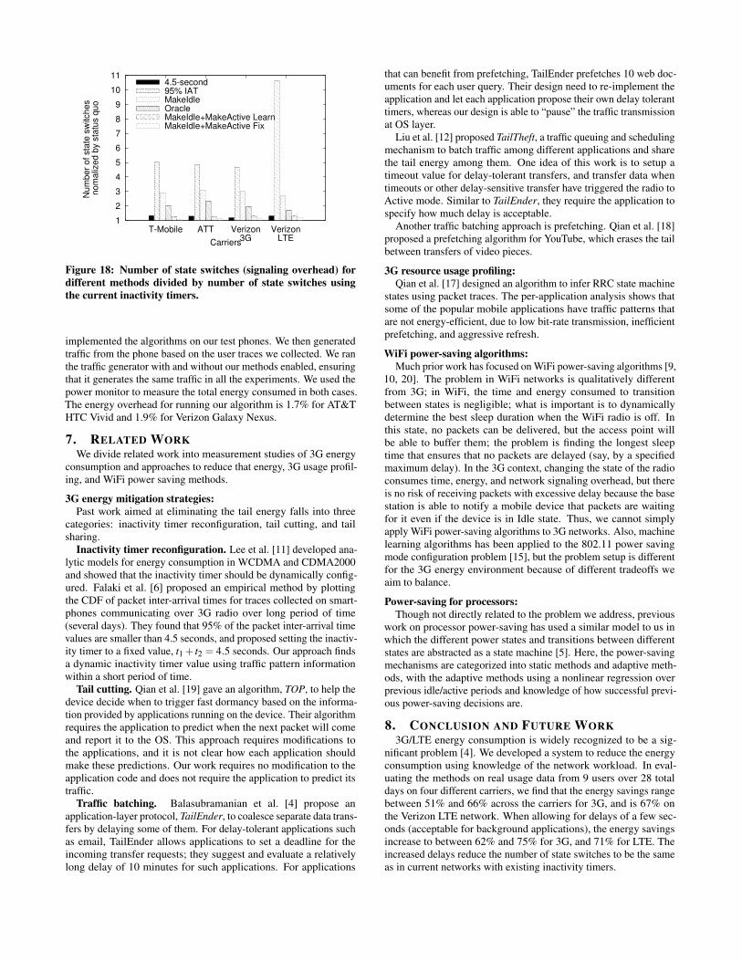
Figure 17 shows the percentage of energy saved compared to thestatus quo. Figure 18 shows the corresponding signaling overhead.We find that the “MakeIdle+MakeActive” method outperforms the“4.5-second tail” method in all the carrier settings. Figure 18 showsthe number of state switches (proportional to signaling overhead) ofdifferent schemes divided by the number of state switches withoutusing any scheme.

The maximum signaling overhead for MakeIdle is less than 3.1×the baseline where no fast dormancy is triggered. For “MakeI-

0

20

40

60

80

100

T-Mobile ATT Verizon3G

VerizonLTE

En

erg

y S

ave

d (

%)

Carriers

4.5-second95% IATMakeIdleOracleMakeIdle+MakeActive LearnMakeIdle+MakeActive Fix

Figure 17: Energy saved for different carrier parameters us-ing different methods. For “MakeIdle”, the maximum gain is67% in Verizon LTE netwrok. For “MakeIdle+MakeActive”,the maximum gain is 75% achieved in Verizon 3G.

dle+MakeActive”, the signaling overhead reduces to only 1.33× orless, a 62% reduction from the previous 3.1×, and is close to thesignaling overhead of “4.5-second tail”. The session delays broughtby MakeActive are listed in Table 3.

In both Figure 17 and 18, the result shown as MakeIdle hasno traffic batching, which corresponds to the case when all thetraffic is treated as delay-sensitive, for example, web browsing. TheMakeActive method is disabled in this case to make sure that theuser’s experience is not adversely affected. One possible methodto decide when to disable MakeActive is for the control modulemaintain a list of delay-sensitive or interactive applications; whenany of these applications is running in the foreground, the systemdisables MakeActive.

Even without MakeActive, the reduction in energy consumptionis still significant in all the 4 carrier settings. The maximum gainis for Verizon LTE, where MakeIdle save 67% energy over statusquo. With MakeIdle, the maximum gain is Verizon 3G, where theenergy saving reaches 75%, and the corresponding median delay is4.48 seconds.

6.6 Energy overhead of running algorithmsTo measure the Energy overhead of running our methods, we

Network Psnd Prcv Pt1 Pt2 t1 t2T-Mobile 3G 1202 737 445 343 3.2 16.3AT&T HSPA+ 1539 1212 916 659 6.2 10.4Verizon 3G 2043 1177 1130 1130 9.8 0Verizon LTE 2928 1737 1325 - 10.2 -

Table 2: Power and inactivity timer values for different net-works. Power values are in mW, times are in seconds.

Network Mean Delay Median DelayT-Mobile 3G 5.11 5.11AT&T HSPA+ 4.80 4.65Verizon 3G 4.67 4.48Verizon LTE 4.62 4.38

Table 3: The mean and median session delays brought byMakeIdle for different carriers (in seconds).

1

2

3

4

5

6

7

8

9

10

11

T-Mobile ATT Verizon3G

VerizonLTE

Nu

mb

er

of

sta

te s

witch

es

no

ma

lize

d b

y s

tatu

s q

uo

Carriers

4.5-second95% IATMakeIdleOracleMakeIdle+MakeActive LearnMakeIdle+MakeActive Fix

Figure 18: Number of state switches (signaling overhead) fordifferent methods divided by number of state switches usingthe current inactivity timers.

implemented the algorithms on our test phones. We then generatedtraffic from the phone based on the user traces we collected. We ranthe traffic generator with and without our methods enabled, ensuringthat it generates the same traffic in all the experiments. We used thepower monitor to measure the total energy consumed in both cases.The energy overhead for running our algorithm is 1.7% for AT&THTC Vivid and 1.9% for Verizon Galaxy Nexus.

7. RELATED WORKWe divide related work into measurement studies of 3G energy

consumption and approaches to reduce that energy, 3G usage profil-ing, and WiFi power saving methods.

3G energy mitigation strategies:Past work aimed at eliminating the tail energy falls into three

categories: inactivity timer reconfiguration, tail cutting, and tailsharing.

Inactivity timer reconfiguration. Lee et al. [11] developed ana-lytic models for energy consumption in WCDMA and CDMA2000and showed that the inactivity timer should be dynamically config-ured. Falaki et al. [6] proposed an empirical method by plottingthe CDF of packet inter-arrival times for traces collected on smart-phones communicating over 3G radio over long period of time(several days). They found that 95% of the packet inter-arrival timevalues are smaller than 4.5 seconds, and proposed setting the inactiv-ity timer to a fixed value, t1 + t2 = 4.5 seconds. Our approach findsa dynamic inactivity timer value using traffic pattern informationwithin a short period of time.

Tail cutting. Qian et al. [19] gave an algorithm, TOP, to help thedevice decide when to trigger fast dormancy based on the informa-tion provided by applications running on the device. Their algorithmrequires the application to predict when the next packet will comeand report it to the OS. This approach requires modifications tothe applications, and it is not clear how each application shouldmake these predictions. Our work requires no modification to theapplication code and does not require the application to predict itstraffic.

Traffic batching. Balasubramanian et al. [4] propose anapplication-layer protocol, TailEnder, to coalesce separate data trans-fers by delaying some of them. For delay-tolerant applications suchas email, TailEnder allows applications to set a deadline for theincoming transfer requests; they suggest and evaluate a relativelylong delay of 10 minutes for such applications. For applications

that can benefit from prefetching, TailEnder prefetches 10 web doc-uments for each user query. Their design need to re-implement theapplication and let each application propose their own delay toleranttimers, whereas our design is able to “pause” the traffic transmissionat OS layer.

Liu et al. [12] proposed TailTheft, a traffic queuing and schedulingmechanism to batch traffic among different applications and sharethe tail energy among them. One idea of this work is to setup atimeout value for delay-tolerant transfers, and transfer data whentimeouts or other delay-sensitive transfer have triggered the radio toActive mode. Similar to TailEnder, they require the application tospecify how much delay is acceptable.

Another traffic batching approach is prefetching. Qian et al. [18]proposed a prefetching algorithm for YouTube, which erases the tailbetween transfers of video pieces.

3G resource usage profiling:Qian et al. [17] designed an algorithm to infer RRC state machine

states using packet traces. The per-application analysis shows thatsome of the popular mobile applications have traffic patterns thatare not energy-efficient, due to low bit-rate transmission, inefficientprefetching, and aggressive refresh.

WiFi power-saving algorithms:Much prior work has focused on WiFi power-saving algorithms [9,

10, 20]. The problem in WiFi networks is qualitatively differentfrom 3G; in WiFi, the time and energy consumed to transitionbetween states is negligible; what is important is to dynamicallydetermine the best sleep duration when the WiFi radio is off. Inthis state, no packets can be delivered, but the access point willbe able to buffer them; the problem is finding the longest sleeptime that ensures that no packets are delayed (say, by a specifiedmaximum delay). In the 3G context, changing the state of the radioconsumes time, energy, and network signaling overhead, but thereis no risk of receiving packets with excessive delay because the basestation is able to notify a mobile device that packets are waitingfor it even if the device is in Idle state. Thus, we cannot simplyapply WiFi power-saving algorithms to 3G networks. Also, machinelearning algorithms has been applied to the 802.11 power savingmode configuration problem [15], but the problem setup is differentfor the 3G energy environment because of different tradeoffs weaim to balance.

Power-saving for processors:Though not directly related to the problem we address, previous

work on processor power-saving has used a similar model to us inwhich the different power states and transitions between differentstates are abstracted as a state machine [5]. Here, the power-savingmechanisms are categorized into static methods and adaptive meth-ods, with the adaptive methods using a nonlinear regression overprevious idle/active periods and knowledge of how successful previ-ous power-saving decisions are.

8. CONCLUSION AND FUTURE WORK3G/LTE energy consumption is widely recognized to be a sig-

nificant problem [4]. We developed a system to reduce the energyconsumption using knowledge of the network workload. In eval-uating the methods on real usage data from 9 users over 28 totaldays on four different carriers, we find that the energy savings rangebetween 51% and 66% across the carriers for 3G, and is 67% onthe Verizon LTE network. When allowing for delays of a few sec-onds (acceptable for background applications), the energy savingsincrease to between 62% and 75% for 3G, and 71% for LTE. Theincreased delays reduce the number of state switches to be the sameas in current networks with existing inactivity timers.

The key idea in this paper is to adapt the state of the radio tonetwork traffic. To put the 66% saving (without any delays) or 75%saving (with delay) in perspective, we note that according to theNexus S specifications, the reduction in lifetime from using the 3Gradio instead of 2G is 7.3 hours; while it is not clear what applicationmix produces these numbers, one might speculate that saving 66%of the energy might correspond to an increase in lifetime by about66% of 7.3 hours, or about 4.8 hours.

There are two areas for future work. First, studying the effects oftriggering fast dormancy on the base station side would be useful,considering issues such as handling multiple phones triggering thefeature, and whether the base station can actively help the phone tomake decisions on fast dormancy by buffering incoming traffic forthe phone. Second, extending the system to include server or basestation functions to coordinate with the mobile device to furtherreduce energy consumption.

9. ACKNOWLEDGMENTSWe thank Katrina LaCurts, Lenin Ravindranath, Keith Winstein,

Jonathan Perry, and Raluca Ada Popa for useful comments on ear-lier versions of this paper. We also thank the reviewers and ourshepherd, Srikanth Krishnamurthy, for their insightful comments.This material is based upon work supported by the National ScienceFoundation under Grant No. CNS-0931550.

10. REFERENCES

[1] 3GPP Release 7: UE Fast Dormancy behavior, 2007. 3GPPdiscussion and decision notes R2-075251.

[2] 3GPP Release 8: 3GPP TS 25.331, 2008.[3] Data Service Options for Spread Spread Spectrum Systems:

Service Options 33 and 66, May 2006.[4] N. Balasubramanian, A. Balasubramanian, and

A. Venkataramani. Energy consumption in mobile phones: Ameasurement study and implications for network applications.In Internet Measurement Conference, 2009.

[5] L. Benini, A. Bogliolo, and G. D. Micheli. A survey of designtechniques for system-level dynamic power management. VeryLarge Scale Integration (VLSI) Systems, IEEE Transactionson, 8(3):299 –316, june 2000.

[6] H. Falaki, D. Lymberopoulos, R. Mahajan, S. Kandula, andD. Estrin. A First Look at Traffic on Smartphones. In InternetMeasurement Conference, 2010.

[7] M. Herbster and M. K. Warmuth. Tracking the best expert.Machine Learning, 32:151–178, 1998.

[8] J. Huang, F. Qian, A. Gerber, Z. M. Mao, S. Sen, andO. Spatscheck. A close examination of performance andpower characteristics of 4g lte networks. In MobiSys, 2012.

[9] R. Krashinsky and H. Balakrishnan. Minimizing Energy forWireless Web Access with Bounded Slowdown. In MobiCom,2002.

[10] R. Krashinsky and H. Balakrishnan. Minimizing Energy forWireless Web Access with Bounded Slowdown. ACMWireless Networks, 11(1–2):135–148, Jan. 2005.

[11] C.-C. Lee, J.-H. Yeh, and J.-C. Chen. Impact of inactivitytimer on energy consumption in WCDMA and CDMA2000.In IEEE Wireless Telecomm. Symp.(WTS), 2004.

[12] H. Liu, Y. Zhang, and Y. Zhou. TailTheft: Leveraging thewasted time for saving energy in cellular communications. InMobiArch, 2011.

[13] Monsoon power monitor. http://www.msoon.com/LabEquipment/PowerMonitor/.

[14] C. Monteleoni. Online learning of non-stationary sequences.In AI Technical Report 2003-011, S.M. Thesis, Artificial

Intelligence Laboratory, Massachusetts Institute ofTechnology, May 2003.

[15] C. Monteleoni, H. Balakrishnan, N. Feamster, and T. Jaakkola.Managing the 802.11 energy/performance tradeoff withmachine learning. Technical Report MIT-LCS-TR-971, MITCSAIL, 2004.

[16] C. Monteleoni and T. Jaakkola. Online learning ofnon-stationary sequences. In Neural Information ProcessingSystems 16, Vancouver, Canada, December 2003.

[17] F. Qian, Z. Wang, A. Gerber, Z. Mao, S. Sen, andO. Spatscheck. Profiling resource usage for mobileapplications: a cross-layer approach. In MobiSys, 2011.

[18] F. Qian, Z. Wang, A. Gerber, Z. M. Mao, S. Sen, andO. Spatscheck. Characterizing radio resource allocation for3G networks. In Internet Measurement Conference, 2010.

[19] F. Qian, Z. Wang, A. Gerber, Z. M. Mao, S. Sen, andO. Spatscheck. TOP: Tail Optimization Protocol For CelluarRadio Resource Allocation. In ICNP, 2010.

[20] T. Simunic, L. Benini, P. W. Glynn, and G. D. Micheli.Dynamic power management for portable systems. InMobiCom, 2000.

[21] J.-H. Yeh, J.-C. Chen, and C.-C. Lee. Comparative Analysisof Energy-Saving Techniques in 3GPP and 3GPP2 Systems.IEEE Trans. on Vehicular Technology, 58(1):432 –448, Jan.2009.

[22] J.-H. Yeh, C.-C. Lee, and J.-C. Chen. Performance analysis ofenergy consumption in 3GPP networks. In IEEE WirelessTelecomm. Symp. (WTS), 2004.

APPENDIXHere we show how bank of experts works. We bound the maximumdelay to n seconds. Each expert “proposes” a delay value Ti:

Ti = i, i ∈ 1 . . .n.

The output of the algorithm is the weighted average over all theexperts:

Tt =n

∑i=1

pt(i)Ti

For each iteration of the updates, the algorithm calculates theprobability of each possible hidden state (in our case, the identityof the expert) based on some observation yt . Here, we can definethe probability of predicting observation yt as P(yt |Ti) = e−L(i,t).The observation is the number of sessions we batched at time t,and L(i, t) is the loss function. Then we can apply the followingequation to get the weight pt(i):

pt(i) =1Zt

n

∑j=1

pt−1( j)e−L( j,t−1) P(i| j,α).

Here, Zt is a normalization factor that makes sure ∑i pt i = 1.The P(i| j,α) shows the probability of switching between experts.There are different versions to solve this part. The one we chose [7]supports switching between the experts and is suitable for caseswhere the observation may change rapidly, which matches the burstycharacter of network traffic. P(i| j,α) is defined as:

P(i| j,α) =

{(1−α) i = j

α

n−1 i 6= j

0≤ α ≤ 1 is a parameter that determines how quickly the algo-rithm changes the best experts. α close to 1 means the networkcondition changes rapidly and the best expert always changes. One

problem with this algorithm is that it is hard to choose a good α .In reality, α should not be a fixed value since the network trafficpattern may change rapidly or remain stationary. We use a moreadaptive algorithm, Learn-α [14, 16], to dynamically choose α .

The basic idea is to first assign m α-experts and use the algorithmabove to learn the proper value of α in each iteration, and then usethe up-to-date α to learn Tt [14, 16]. The final equation for this“two-layer learning” is:

Tt =m

∑j=1

n

∑i=1

p′t( j)pt, j(i)Ti (3)

Here, p′t( j) is the weight for the jth α-expert, which is given by:

p′t( j) =1Zt

p′t−1( j)e−L(α j ,t−1) (4)

This equation shows that p′t( j) is updated from the previous valuep′t−1( j); the initial values are: p′1( j) = 1/m. −L(α j, t−1) is the α

loss function, defined as:

L(α j, t) =− logn

∑i=1

pt, j(i)e−L(i,t) (5)

Here, L(i, t) is the loss function, discussed in §5.2. t is the presenttime; the loss function value for the current iteration is calculatedfrom information learned at time t−1.