integration of top-down and bottom-up information …integration of top-down and bottom-up...
TRANSCRIPT

General rights Copyright and moral rights for the publications made accessible in the public portal are retained by the authors and/or other copyright owners and it is a condition of accessing publications that users recognise and abide by the legal requirements associated with these rights.
Users may download and print one copy of any publication from the public portal for the purpose of private study or research.
You may not further distribute the material or use it for any profit-making activity or commercial gain
You may freely distribute the URL identifying the publication in the public portal If you believe that this document breaches copyright please contact us providing details, and we will remove access to the work immediately and investigate your claim.
Downloaded from orbit.dtu.dk on: Apr 09, 2020
Integration of top-down and bottom-up information for audio organization and retrieval
Jensen, Bjørn Sand
Publication date:2012
Document VersionPublisher's PDF, also known as Version of record
Link back to DTU Orbit
Citation (APA):Jensen, B. S. (2012). Integration of top-down and bottom-up information for audio organization and retrieval.Kgs. Lyngby: Technical University of Denmark. IMM-PhD-2012, No. 291

Integration of top-down andbottom-up information for audio
organization and retrieval
Bjørn Sand Jensen
Kongens Lyngby 2012IMM-PHD-2012-291

Technical University of DenmarkInformatics and Mathematical ModellingBuilding 321, DK-2800 Kongens Lyngby, DenmarkPhone +45 45253351, Fax +45 [email protected]
IMM-PHD: ISSN 0909-3192
Summary
The increasing availability of digital audio and music calls for methods andsystems to analyse and organize these digital objects. This thesis investigatesthree elements related to such systems focusing on the ability to represent andelicit the user’s view on the multimedia object and the system output. The aimis to provide organization and processing, which aligns with the understandingand needs of the users.
Multimedia, including audio and music, is often characterized by large amountof heterogeneous information, and the first element investigated in the the-sis concerns the integration of such heterogeneous and multimodal informationsources based on latent Dirichlet allocation (LDA). The model is used to in-tegrate bottom-up features (reflecting timbre, loudness, tempo and chroma),meta-data aspects (lyrics) and top-down aspects, namely user generated openvocabulary tags. The model and representation is evaluated on the auxiliarytask of genre classification.
Eliciting the subjective representation and opinion of users is an important andchallenging element in building personalized systems. The thesis contributeswith a setup for modelling and elicitation of preference and other cognitive as-pects with focus on audio applications. The setup is based on classical regressionand choice models placed in the framework of Gaussian processes, which pro-vides flexible non-parametric Bayesian models. The setup consist of a number oflikelihood functions suitable for modelling both absolute ratings (direct scaling)and comparative judgements (indirect scaling). Inference is typically performedby analytical approximation methods, including the Laplace approximation andexpectation propagation. In order to minimize the cost of the often expensive

ii
and lengthy experimentation, sequential experiment design or active learning issupported as an integrated part of the setup. The setup is applied in the field ofmusic emotion modelling and optimization of a parametric audio system bothwith high-dimensional input spaces.
The final element considered in the thesis, concerns the general context of users,such as location and social context. This is important in understanding userbehavior and in determining the users current information needs. The thesisinvestigates the predictability of the user context, in particular location, basedon information theoretic bounds and a particular experimental approach basedon context sensing using the ubiquitous mobile phone.

Resume (in Danish)
Den stigende tilgængelighed og brug af digitale medier kræver metoder og sys-temer til at forsta og organisere sadanne digitale objekter og det ideelt pa enmade, der er i trad med brugernes forstaelse, forventninger og behov. Denneafhandling undersøger tre elementer i sadanne systemer som alle vedrører sys-temets evne til at repræsentere og frembringe brugerens syn pa objektet ellersystemets output.
Multimedie, inklusiv lyd og musik, er ofte karakteriseret ved store mængdeaf heterogene informationskilder, og det første element, der er undersøges iafhandlingen, er integration af sadanne informationskilder ved hjalp af LatentDirichlet Allocation (LDA). Modellen anvendes til at integrere bottom-up as-pekter (timbre, loudness, tempo og chroma features), metadata aspekter (lyrik)samt top-down aspekter i form af brugergenererede annotationer. Modellen ogrepræsentationen evalueres blandt andet pa sin even til at repræsentere genre.
Modellering og eksperimentel frembringelse af en brugers interne repræsentationog forstaelse af for eksempel musik er en generel udfordring i multimediesystmerog andre applikationer. Afhandlingen bidrager med en opsætning til modeller-ing og frembringelse af præference og andre kognitive aspekter. Opsætningener baseret pa klassiske regressions- og beslutningsmodeller i rammerne af Gaus-siske processer, hvilket resulterer i en række ikke-parametriske Bayesianske mod-eller. Opsætningen bestar af en række likelihood funktioner, der er egende til atmodellere bade brugeres absolutte vurderinger eller parrerede sammenligninger.Inferens i disse modeller er typisk udørt gennem analytiske approksimationsme-toder sasom Laplace-approksimationen og expectation propagation. For at min-imere den ofte kostbare eksperimentelle forsøgtid, er sekventiel eksperimentel

iv
design understøttet som en integeret del af opsætningen. Metoderne anvendesinden for modellering af følelser i musik og brugeroptimering af et parametriskaudio system med høj-dimensionelle data.
Det sidste aspekt, der er undersøgt, relaterer sig til brugerens generelle kontekst,som placering og social kontekst, hvilket er vigtigt for forstaelsen af brugerad-færd og til afdækning af brugernes aktuelle informationsbehov. Afhandlingenundersøger forudsigeligheden af brugerens kontekst, navnlig placering, baseretpa informationsteoretiske grænser og en bestemt eksperimentel tilgang baseretpa indsamling af data fra den allestedsnærværende mobiltelefon.

Preface
This thesis was prepared at The Department of Informatics and Mathemati-cal Modeling (IMM), The Technical University of Denmark (DTU), in partialfulfillment of the requirements for acquiring the Ph.D. degree at DTU.
The project was funded by DTU, initiated April 2009 and completed December2012. Throughout the period, the project was supervised by associate professorJan Larsen and by co-supervisor professor Lars Kai Hansen.
The thesis reflects the research part of the project. It consists of an summaryreport in combination with a collection of published and submitted researchpapers written during the period and published during the project period (orimmediately thereafter 1).
The project is motivated by the challenges involved in processing, modellingand organization of multimedia in particular in systems where users plays anintegral role. This is a highly cross-disciplinary field including elements fromdigital signal processing, human-computer interaction, cognitive modelling andmachine learning. The thesis therefore consist of contributions originating inthree different research fields of course with some overlap. It is therefore theaim of the summary report to give a coherent and general overview of the con-tributions from a system perspective. Hence, this summary report is thereforenot an exhaustive walk-through of all applied methods and detailed derivations,but an attempt to place the contributions in an overall and general context ofuser driven machine learning systems.
1Note that the final version of the report has been updated with the published versions ofthe papers originally indicated as submitted

vi
The report further refrains from describing well-known methods such as Ex-pectation Maximization, Support Vector Machines and K-means, and simplyprovide textbook reference for standard methods well-described in textbooks orelsewhere. As a consequence it is assumed that the reader is familiar with basicprobability theory and its application in machine learning.
Bjørn Sand JensenJanuary 14th, 2013

Dissemination
Papers (peer-reviewed)
A Bjørn Sand Jensen, Jakob Eg Larsen, Kristian Jensen, Jan Larsen, andLars Kai Hansen. Estimating Human Predictability from Mobile SensorData. IEEE International Workshop on Machine Learning for SignalProcessing, Pages) 196-201, 2010. DOI:10.1109/MLSP.2010.5588997
C Bjørn Sand Jensen, Jens Brehm Nielsen, and Jan Larsen. Efficient Prefer-ence Learning with Pairwise Continuous Observations and Gaussian Pro-cesses. IEEE International Workshop on Machine Learning for SignalProcessing. Pages 1-6, 2011. DOI:10.1109/MLSP.2011.6064616
D Bjørn Sand Jensen, Javier Saez Gallego and Jan Larsen. A PredictiveModel of Music Preference using Pairwise Comparisons. InternationalConference on Acoustics, Speech, and Signal Processing (ICASSP), Pages1977-1980, 2012. DOI:10.1109/ICASSP.2012.6288294
F Jens Madsen, Jens Brehm Nielsen, Bjørn Sand Jensen and Jan Larsen.Modeling Expressed Emotions in Music using Pairwise Comparisons. 9thInternational Symposium on Computer Music Modeling and Retrieval(CMMR). Pages 526-533, 2012.
E Jens Madsen, Bjørn Sand Jensen, Jan Larsen and Jens Brehm Nielsen.Towards Predicting Expressed Emotion in Music from Pairwise Compar-isons. 9th Sound and Music Computing Conference. Pages 350-357,2012.

viii
G Jens Brehm Nielsen, Bjørn Sand Jensen and Jan Larsen. Pseudo In-puts For Pairwise Learning With Gaussian Processes IEEE InternationalWorkshop on Machine Learning for Signal Processing, Pages 1-6, 2012DOI:10.1109/MLSP.2012.6349812
H Bjørn Sand Jensen, Rasmus Troelsgaard, Jan Larsen and Lars Kai HansenTowards a universal representation for audio information retrieval andanalysis International Conference on Acoustics, Speech, and Signal Pro-cessing (ICASSP), Pages 3168-3172, 2013. DOI:10.1109/ICASSP.2013.6638242.
I Jens Brehm Nielsen, Bjørn Sand Jensen and Toke Jansen Hansen Person-alized Audio Systems - a Bayesian approach Audio Engineering SocietyConvention 135, Pages 1-10, 2013. 2
J Bjørn Sand Jensen, Jens Brehm Nielsen and Jan Larsen. Bounded Gaus-sian Process Regression. IEEE International Workshop on Machine Learn-ing for Signal Processing, Pages 1-6, 2013 DOI:10.1109/MLSP.2013.6661916.3.
Workshop Contributions (peer-reviewed)
B Bjørn Sand Jensen, Jan Larsen, Lars Kai Hansen, Jakob Eg Larsen, andKristian Jensen. Predictability of mobile phone associations. EuropeanConference on Machine Learning : Mining Ubiquitous and Social Envi-ronments Workshop (ECML-MUSE), Pages 1-15, 2010, Peer Reviewed.
MiscellaneousOther papers and software prepared during the project, but not part of thethesis
[4] Tommy S. Alstrøm, Bjørn S. Jensen, Mikkel N. Schmidt, Natalie V. Koste-sha and Jan Larsen. Haussdorff and Hellinger for Colorimetric SensorArray Classification IEEE International Workshop on Machine Learningfor Signal Processing, Pages 1-6, 2012. DOI:10.1109/MLSP.2012.6349724
· Bjørn Sand Jensen & Jens Brehm NielsenMatlab R© Toolbox for Preference Learning with Gaussian Proceses- with documentation, 2013
2Note that this paper was originally included in the thesis as submitted (and includedin the thesis) as: Jens Brehm Nielsen, Bjørn Sand Jensen and Toke Jansen Hansen, Fastand flexible elicitation of preference in complex audio systems, International Conference onAcoustics, Speech, and Signal Processing (ICASSP), 2013, but subsequently published as I
3Note that this paper was originally included in the thesis as a technical report entitled:On Bounded Regression with Gaussian Processes but was subsequently published as J

Acronyms
AIC Akaike information criterion
ANOVA Analysis of variance
ARD Automatic Relevance Determination
BIC Bayesian Information Criterion
BTL Bradley Terry Luce
BFGS Broyden Fletcher Goldfarb Shanno
CCA Canonical Correlation Analysis
CV Cross-validation
DCT Discrete cosine transform
DACE Design and analysis of computer experiments
EVOI Expected Value of information
EM Expectation Maximization
EM Expectation Propagation
FFT Fast fourier transform
FI(T)C Fully Independent (Training) Conditional
GLM Generalized Linear Models
GMM Gaussian Mixture Model

x Acronyms
GP Gaussian Process
GEVIO Gradient of EVIO
HB Hierarchical Bayes
HDP Hierarchical Dirichlet process
IVM Informative Vector Machine
KL Kullback-Leibler
LSA Latent Semantic Analysis
LDA Latent Dirichlet Allocation
EP Expectation Propagation
KNN k-nearest neighbor
LOO Leave-One-Out
LOO-CV Leave-One-Out Cross validation
LZ Lempel-Ziv
MSE Mean Squared Error
MAE Mean Absolute Error
MAP Maximum-a-Posteriori
MAP-II Maximum-a-Posteriori Type-II (estimation)
MCMC Markov Chain Monte Carlo
MI Mutual Information
MIR Music Information Retrieval
MKL Multiple Kernel Learning
MFCC Mel-frequency cepstral coefficients
ML Maximum Likelihood
ML-II Maximum Likelihood Type-II (estimation)
MSD Million Song Dataset
MTK Multi-task kernel
NN (Artificial) Neural Network

xi
NMF Non-negative matrix factorization
NMI Normalized Mutual Information
PCA Principal Component Analysis
PI(T)C Partial Independent (Training) Conditional
pLSA Probabilistic Latent Semantic Analysis
P/L Probit/Logit)
PLP Perceptual linear predictive (analysis/encoding)
PJK Pairwise Judgement Kernel
PPK Probability Product Kernel
SSK Semi-Supervised Kernel
SVM Support Vector Machine
SVMrank Support Vector Machine for ranking
RVM Relevance Vector Machine
THOMP Thompson (sampling)
UCB Upper Confidence Bound
VB Variational Bayes
VOI Value of information
VQ Vector Quantization

xii

Notation
The following contains a list of common notation and symbols used throughoutthe report, which may differ slightly from the contributions in order to providea coherent notation across different focus areas. Variations and specialized usemay occur which is made clear from the context.
Various sets of variables and observations
R The reals.Z Integers.N Natural numbers (including zero).X Domain of the input variable / input space.Y Domain of the output variable / output space.X A set. Typically of input instances from X. Typically index
with nY A set. Typically of outputs from Y. Typically indexed with
kV A set. Typically used to denote a vocabulary of words
indexed by v.D A set. A joint collection of inputs and outputs, D = {X ,Y},
so a dataset.C A (choice) set of inputs. A subset from X used in a specific
likelihood.E An experiment set. A subset from X

xiv Notation
Size/count parameters:
D Dimension of input space XN Number of inputs, N = |X | or as or general count, typically
with an informative subscript.K Number of observations/experiment K = |Y|. .C = |C| Size of choice set. Typically indexed with k.M Number of data modalities or as a general count. Typically
indexed with mV = |V| Size of a given vocabulary, i.e. V words in the vocabulary.E = |E| Size of (candidate) experiment set.Z Number of latent components, e.g. number of Gaussian
components or topics. Related index variable is z.S Number of songs, typically indexed with s. Note that S is
also used to denote various information theoretic measuresuch as entropy, however never in the same context as song.
Variables and observations:
y A output variable/observation (used in supervised contextonly)
y A multidimensional output variable / observation (used insupervised context only)
X A random variable (used when required to differential be-tween the variable itself and the outcome which is clearfrom context)
x, w (Multi-dimensional) input (or outcome when required todifferentiate between outcome and variable which is clearfrom context)
X, W A collection of inputs N ×Dx∗/x∗ A test inputw∗/w∗
y∗/y∗ A test output

xv
Probabilities and distributionsThe notation does not distinguish between probability and probability densities,where it is clear from the context. Capital letters is used for the variable itselfwhere it is advantageous to differentiate (Chapter 4) and in following list todifferentiate between variable and outcome).
P (X = x) The probability that the random variable X takes on agiven value x. P (X) ∈ [0; 1].
p (x|θ) A probability density parameterized by elements in θP (X = x|Y = y) A conditional probability probability where X is condition
on another random variable, Yp (y|x) A conditional probability density function (or condition
probability, which is clear from context)E(X) Expectation of a random variable, X.V(X) Second order moment of the random variable X, i.e. vari-
ance. Also used to denote covariance.

xvi Notation
Distributions, processes and related functions:
A stochastic process is a collection of random variables Xi indexed by i X ={X1, X2, ..., XN}. In the report a Gaussian process considered from a func-tion viewpoint a the following notation is employed, and using an informalnotation, a Gaussian process is then denoted f = {f1, f2, ..., fN} or f(·) ={f(x1), f(x2), ..., f(xN )}, thus fi , f(xi) being the individual random vari-ables. It is noted that the Gaussian process is defined for all x ∈ X, i.e. inprinciple infinite, but we usually consider a finite subset through a vector f ofthe function evaluated a finite set of inputs, i.e., f = [f(x1), f(x2), ..., f(xN )],resulting in a tractable finite multi-variate Gaussian distribution.
N (x|µ,Σ) Normal/Gaussian Distribution (used interchangeably) [26,App. B]
N (µ,Σ)Φ (z) Cumulative Gaussian, with mean 0 and standard deviation
1Φ−1 (z) Probit function. Inverse cumulative Gaussian.Beta (α, β) A standard two parameter beta distributionCategorical(λ) A categorical distribution [26]. A multinomial distrbution
with only one draw. Parameterized by the probabilities λ.Dirichlet(α) A Dirichlet distrbution parameterized by the concentration
parameter α [26, App. B]TG(µ, σ) Standard truncated Gaussian distribution usually with sup-
port in [0, 1]Truncated G.k(x, x′) Covariance function, co-defining a Gaussian processm(x) Mean function, co-defining a Gaussian processK or KXX Covariance marix with elements k(x, x′) between all train-
ing inputs.kr Covariance vector between all traning inputs and a test
input xr.
Information theory
S (X) (Shannon) Entropy of the random variable XS (X|Y = y) Conditional entropy of the random variable x conditioned
on the random variable Y taking a particular valueS (X|Y ) Conditional entropy of the random variable S conditioned
on the random variable Y - or a dataset in some cases.

xvii

xviii Contents

Contents
Summary i
Resume (in Danish) iii
Preface v
Dissemination vii
Acronyms ix
Notation xiii
Contents xviii
1 Introduction 11.1 Focus Areas . . . . . . . . . . . . . . . . . . . . . . . . . . . . . . 51.2 Contributions . . . . . . . . . . . . . . . . . . . . . . . . . . . . . 81.3 Structure . . . . . . . . . . . . . . . . . . . . . . . . . . . . . . . 9
2 Computational Representation of Music 112.1 The Audio Object: Signal and Metadata . . . . . . . . . . . . . . 132.2 Bottom-Up View . . . . . . . . . . . . . . . . . . . . . . . . . . . 15
2.2.1 Song Level Representation . . . . . . . . . . . . . . . . . . 172.3 Top-Down View . . . . . . . . . . . . . . . . . . . . . . . . . . . . 212.4 Joining Views . . . . . . . . . . . . . . . . . . . . . . . . . . . . . 25
2.4.1 Example: Multimodal Integration . . . . . . . . . . . . . 262.4.2 Multimodal Latent Dirichlet Allocation . . . . . . . . . . 272.4.3 Discussion and Extensions . . . . . . . . . . . . . . . . . . 31
2.5 Summary . . . . . . . . . . . . . . . . . . . . . . . . . . . . . . . 32

xx CONTENTS
3 Preference Learning with Gaussian Processes 33
3.1 Gaussian Processes . . . . . . . . . . . . . . . . . . . . . . . . . . 37
3.1.1 Mean & Covariance Functions . . . . . . . . . . . . . . . . 40
3.1.2 Inference & Model Selection . . . . . . . . . . . . . . . . . 43
A two step approach: . . . . . . . . . . . . . . . . 43
Hyperparameters and Model Selection . . . . . . . 47
3.2 Rating & Ranking with GPs . . . . . . . . . . . . . . . . . . . . . 49
3.2.1 Relative-Discrete-Pairwise-Probit/Logit Model . . . . . . 50
3.2.2 Relative-Continuous-Pairwise-Beta Model . . . . . . . . . 52
3.2.3 Absolute-Continuous-Bounded Beta Model . . . . . . . . 53
3.2.4 Releative-Discrete-General Bradley-Terry-Luce and Plackett-Luce . . . . . . . . . . . . . . . . . . . . . . . . . . . . . . 54
3.2.5 Additional Models . . . . . . . . . . . . . . . . . . . . . . 55
3.3 Sequential Design & Sparsity . . . . . . . . . . . . . . . . . . . . 56
3.3.1 Sequential Design & Natural Sparsity . . . . . . . . . . . 57
3.3.2 Induced Sparsity . . . . . . . . . . . . . . . . . . . . . . . 64
3.3.2.1 ...for Pairwise Likelihoods . . . . . . . . . . . . . 64
3.4 Evaluation Methods . . . . . . . . . . . . . . . . . . . . . . . . . 65
3.5 Alternatives . . . . . . . . . . . . . . . . . . . . . . . . . . . . . . 68
3.6 Summary & Perspectives . . . . . . . . . . . . . . . . . . . . . . 68
4 Predictability of User Context 71
4.1 Basic Measures of Information . . . . . . . . . . . . . . . . . . . 72
4.1.1 Entropy Rate Estimation . . . . . . . . . . . . . . . . . . 73
4.2 Bounds on Predictability . . . . . . . . . . . . . . . . . . . . . . . 74
4.2.1 Upper Bound . . . . . . . . . . . . . . . . . . . . . . . . . 75
4.2.2 Lower Bound . . . . . . . . . . . . . . . . . . . . . . . . . 75
4.3 Summary . . . . . . . . . . . . . . . . . . . . . . . . . . . . . . . 76
5 Summary & Conclusion 77
A Estimating Human Predictability from Mobile Sensor Data 81
B Predictability of Mobile Phone Associations 89
C Effecient Preference Learning with Pairwise Countinious Ob-servation and Gaussian Processes 107
D A Predictive Model of Music Preference using Pairwise Com-parisons 115
E Towards Predicting Expressed Emotion in Music from PairwiseComparisons 121

CONTENTS xxi
F Modeling Expressed Emotions in Music using Pairwise Com-parisons 131
G Pseudo Inputs For Pairwise Learning With Gaussian Processes141
H Towards a Universal Representation for Audio Information Re-trieval and Analysis 149
I Personalized Audio System - a Bayesian Approach 157
J Bounded Gaussian Process Regression 173
Index 181
Bibliography 181

xxii CONTENTS

Chapter 1
Introduction
The growth of the digital multimedia world, in terms of both scale and use,makes it increasingly important to create systems to process and organize digitalmultimedia objects, such as text documents, books, video and audio objectswith the aim to increase the productivity and the satisfaction of the users.The emphasis on the user is especially important in multimedia systems, wherethe information itself has a profound perceptual and cognitive influence on theusers, such as music which has the ability to both move, repel and even healus [185]. It has therefore become an important engineering task to design andbuild systems to store, process and organize multimedia information, designedto be well aligned with the user’s needs and expectations.
The systems considered in this thesis ranges from relatively simple reproductiondevices like personal media players or hearing aids, to more complex organiza-tion and retrieval systems, such as search engines and recommendation services.In the first case, the system task is typically to provide a optimally processedversions of the input conditioned on system parameters. In the second case, thesystem task is essentially to define similarity between user query and objects tobe able to return relevant search results. In order to produce a particular systemresult and output - such as search results, processed audio files or recommenda-tions - a given system often make use of a so called computational representationor mathematical models. This representation essentially defines the similarityand relations between either system parameters or the objects. The only as-
2 Introduction
sumption regarding a system in this context; is that these are designed to beutilized and operated by human subjects: the users. Such users have consciousor unconscious information needs (see e.g. [144][211]), a subjective understand-ing of objects relations and certain expectations to the system response. Wethreat such user related and specific aspects under the general notion of a userrepresentation encompassing the general state of the user, possibly affectedby the current environmentally context of the user such as location and socialcontext. If the computational representation and the user’s representation is notaligned suboptimal system performance is typically encountered. We here de-fine this misalignment as the semantic gap [198]. The overall system goal is tominimize this semantic gap by ensuring that the computational representationis well-aligned with the user’s representation and needs.
Modern computational representations for organization and retrieval includethe latent semantic view of multimedia objects in text mining [55] and music[240, 239, 105], which in a unsupervised manner extracts the latent semanticsof the data in order to provide grouping and organization. The main goal isto provide representations well aligned with general human representations, forwhich reason the term ’cognitive’ components [83] is sometimes preferred. Suchpurely content based and unsupervised representations is here defined as thebottom-up view or a computational low-level representation. Examples ofsuch bottom-up based systems include content based recommendation in forexample image retrieval and music recommendation/similarity [127].
An unsupervised bottom-up representation may provide general alignment withgeneric perceptual and cognitive representations evaluated over the general pop-ulation. However, representation of objects and/or the system output is typi-cally highly subjective and depends on the general state of the user. To obtaina computational representation aligned with the representation of the individ-ual user, it is thus necessary to obtain information regarding the user viewon objects, system output and possibly the user’s environmental context. Inthe simplest case this information may be as simple as providing labels for theobjects, which results in classical supervised machine learning setting (see e.g.[26]. Other examples include reproduction systems such as personal entertain-ment systems, where system parameters are adapted based on user’s indicationof preference. Such consciously expressed information is here defined as a top-down and a computational representation based solely on this view is referredto as high-level representation. Examples of purely top-down driven systems in-clude collaborative filtering, relying only on user’s ratings such as Netflix [166]and Amazon [6]. Slightly more subtle top-down driven systems include musicrecommendation services like last.fm [119]. Here user provided tags can be seenas a conscious wish to express the user’s view on the object or system output.The high-level computational representation can, for example, be obtained bylatent semantic analysis [125], classification or regression models for represent-
3
- content basedprocessing
- content basedfeature extration
Object-content
User
Bott
om
-up
ComputationalRepresentation
High-levelRepresentation
Top-D
ow
n
User Representation
- expressed system view
- expressed system needs
- system parameters- objectmetadata
Semantic Gap
- recieved user view
- recieved user needs
- expressed userview- expressed userneeds
-Low LevelRepresentation
- user context
(2.2)
(2) (I)
(1) (I)
(1) (2.1)
(3) (2.3)
(4)
(2) (2.4) (3)
(2.1)
(1)
(1) (2.4) (3.3.1)
(3) (2.3)
(1)
(1)
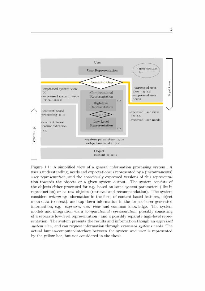
Figure 1.1: A simplified view of a general information processing system. Auser’s understanding, needs and expectations is represented by a (instantaneous)user representation, and the consciously expressed versions of this representa-tion towards the objects or a given system output. The system consists ofthe objects either processed for e.g. based on some system parameters (like inreproduction) or as raw objects (retrieval and recommendation). The systemconsiders bottom-up information in the form of content based features, objectmeta-data (context), and top-down information in the form of user generatedinformation, e.g. expressed user view and common knowledge. The systemmodels and integration via a computational representation, possibly consistingof a separate low-level representation , and a possibly separate high-level repre-sentation. The system presents the results and information though an expressedsystem view, and can request information through expressed systems needs. Theactual human-computer-interface between the system and user is representedby the yellow bar, but not considered in the thesis.

4 Introduction
ing aspects such as categorization (e.g. genre) and preference. Such top-downdriven systems has the possibility to determine a representation based on theuser’s expressed views, namely the user generated data. However, such user gen-erated data is typically a noisy expression of the true user representation dueto subject inconsistencies and drift in the user representation itself, for exampledue to change in user context. The high-level computational representation,therefore, only reflects the expressed version of the user representation; not therepresentation its self. Furthermore, a purely top-down approach suffers fromthe cold-start problem, in which some ratings may be missing for a subset or allobjects (or system outputs).
With the pros and cons of both bottom-up and top-down views, a potentialsolution towards fully bridging the semantic gap seems to be the combinationof both. In combination, the two views is potentially robust to missing andnoisy user generated view, and the lack of individualization in purely bottom-up driven systems. So far the definition of computational representations hasbeen divided to a low- and a high-level representation based on information onwhich they were based. This simply illustrates that such separation is some-times possible and logical on its own. In a combined view, however, simplerepresentation can, for example, include standard classification and regressionmodels. In this case, the bottom-up view is simply used as a input (feature) tothe representation leading to a top-down aspect without the need or requirementfor separate bottom-up and top-down representations1. More subtle systems,which combines the two separate computational representations, include recom-mendation systems which takes into account both content and annotations (forexample in the form of two separate or combined LSA representations). A num-ber of such systems has been proposed for multimedia systems, for examples inimage retrieval [85][187], and in various form in the music information retrieval(MIR) community [188][43][208][240][206].
An important part, not addressed in the so far static description of a system, isthe actual dynamic use of the system, i.e., the interaction taking place betweenthe system and the users. From the user perspective this interaction is theprocess of using the system to obtain a given (potentially unconscious) need,i.e, find relevant webpages or listening to music with the best possible reproduc-tion performance. From the system perspective this is ideally a combinedprocess of a) satisfying the user’s information needs and b) learning and/oradapting the representations in order to achieve the first part. Part a) is givenby the main purpose (as seen from the users) of the system, for example re-trieval/recommendation or reproduction. Part b) is the process of optimizingthe computational representation (of both users and the objects) in an optimal
1One may argue that for example kernel methods require a low-level representation ofthe inputs in the form of a kernel function which on its own defines low-level similarity andrelations, i.e. a representation.
1.1 Focus Areas 5
fashion by obtaining the users top-down view of the objects, object relations,user relation or system results. And potentially (decoding) the context of theusers. Thus, part b) relates to fulfilling the information needs of the system.Fulfilling the systems needs can be done in many ways, i.e, explicitly queryingthe users by requesting annotations - or implicitly by observing the user’s re-sponse to an result such as click-through rates and implicit feedback [10]. Incombination, we refer to part a) and b) as the interactive learning processor simply active learning when the focus is on the algorithmic and not thesystem aspects.
The defining aspect of the systems (and algorithms) is the user. While thereare many open purely technical and algorithmic problems towards the generaland ultimate machine learning system, many challenges relates directly to theusers of the system. This thesis will focus on a few of the many aspects outlinedabove which are outlined in the following section.
1.1 Focus Areas
The ambition in many application domains is to eventually design and constructsystems with many of the appealing properties discusses above. This thesiswill focus on three different, but equally important elements of the generalchallenge, namely a combined computational representation of music, preferencelearning with focus on audio and music - and finally human predictability withrelevance to user context and characterization of human behavior. These aspectsare conceptually outlined below while a more detailed overview and technicalaspects are covered in individual chapters 2 3 4 presenting short introductionsto the different fields and the contributions.
Computational Representations of Music
Multimedia and in particular music has an immense impact on the modern so-ciety in terms of well-being [51][185] and commercial value (e.g. [95][112]). Thelarge boost in music consumption created by the personal and portable devices,such as MP3-players and smartphones, has created the need and demand forservices which organize, recommendation and stream the actual content.
However, few if any of the current music recommendation and retrieval serviceshas truly managed to provide relevant and personal music recommendation andsearch results [43]. This is for example reflected in the way many users still
6 Introduction
discover new music, namely through the ’non-interactive’ radio [171]. Potentialsolutions towards a successful music recommendation and retrieval system (seee.g. [208][43]) is based on the general system outlied in Fig.(1.1). This impliescomputational music representations which are based both on bottom-up audioanalysis and user based top-down views reflecting multiple high-level aspects ofthe music, such as emotion, preference and categorization. In the optimal casethis should be combined with interactive process ensuring that the representa-tion is updated based on changes in environmental and social context.
The aim of this thesis is to investigate a subpart of this ’ideal’ music system.The goal is specifically to investigate models and representations which cancombine the bottom-up view - based on audio content analysis - with a top-down view based on an expressed user view obtained through user annotationannotations. In particular, the aim is to evaluate the representation on therecently published Million Song Dataset which will ensure both scalability ofthe methods and generalization of the results. Secondly, the goal of the thesisis to examine robust and flexible way to represent and elicit cognitive aspectssuch as preference and emotion in music, based on the methods provided by thenext focus area.
Preference Learning with Gaussian processes
Explicit, top-down user ratings and judgements is a major element in manymodern information processing systems such as movie and book recommenda-tion, satisfaction of online web services, implicit user feedback via click-throughrates in online advertising or search engines [10] and skipping behavior in musicplaylists [174].
Such ratings, judgement and feedback represent a general desire from the systemto elicit and understand perceptual and cognitive aspects of the users in order tooptimize system performance. However, robustly eliciting such aspects is oftencomplicated by the aspects themselves, such as preference, which are inherentlydifficult to elicit and represent due to the profound and diverse cognitive effectfor example audio and music has on the users. These issues can often be framedin terms of standard signal detection theory [230] where concepts such as internalnoise, bias and drift can be used to describe the challenges in obtaining robustratings and judgements.
Experimental psychology has dealt with such issues in decades and often relyon relative simple experimental protocols for examining one (or few) effectsin well-controlled situations and analyses the results with standard statisticaltest. The sensormetric field, often applied in the food sciences for optimizing
1.1 Focus Areas 7
products [163], also deals with similar aspects. However this field typically focuson discriminative testing and post-analysing a few, well-defined effects and inparticular, one (or a few) fully controllable variables. In the system view of thisthesis, such methodologies are available only in situations where the aim is topost-optimize explicit system parameters in for example reproduction systems.This does not usually allow for application in interactive systems with manypartly controllable variables as in the case of general preference learning ofmusic and online system optimization.
The goal in this thesis is therefore to investigate and realize a general setupbased on flexible Gaussian processes, applicable in real interactive systems. Itshould be both flexible and robust in eliciting and representing different percep-tual and cognitive aspects, such as preference and cognitive aspects of audio.The aim is therefore is to provide support for different response types, includingdiscrete choices and continuous ratings, suitable for modelling the particular ob-servations originating from different experimental paradigms. To optimize thelearning rate of the system, it is the aim to investigate effective paradigms in-cluding extended versions of classic forced choice paradigms. To further optimizethe learning rate sequential experimental design should also be supported foroptimal experimentation in real applications. It should, in a flexible way, sup-port the many representations relevant to audio and music, including multipleheterogenous data sources potentially modeled by probability density functions.
The realized setup 2 is presented in details in section 3, and documented andapplied in multiple contribution listed in Sec.1.2.
Predictability of User Context
The context in which users interacts with systems and objects has a majorinfluence on both the users representation in terms of needs and understandingof the objects and system output. One major aspect of the user context islocation (others include social context), which can typically be used to improvethe computational representation of the objects of interest.
A intriguing aspect of human context, and in particular location, is to whatdegree it can be predicted based on the past which determines the so-calledpredictability. From an engineering viewpoint this has relevance to resourceallocation and general system optimization, however, the predictability of loca-tion provides a basic view into human behavior by quantifying the repetitivepatterns of human life.
2Developed in collaboration with co-authors.

8 Introduction
The aim of the thesis is to investigate methods for characterizing and examiningthe predictability of subjects, in particular the location aspect sampled using theubiquitous mobile phone. The goal is to quantify the fundamental predictabilityof humans mobility, which characterises each individual user. The methods foraccomplishing this are described in Chapter 4 and the dataset and results arepresented in [B] and [A].
1.2 Contributions
The academic contributions follows the three areas defined above, thus
• The first contribution relates to finding semantic representation of musicby modelling music data by multi-modal Bayesian topic models whichprovides a relatively simple, but widely applicably probabilistic model.Contribution [H] is a study of the million song dataset [20] analysing thealignment between top-down open vocabulary tags with the bottom-uprepresentation. It furthermore examines the predictive power of the jointmodel for genre and style prediction - a classic task MIR task.
• The second and primary group of contributions is in the field of ranking,rating and preference learning. The thesis contributes with a numberof modelling extensions and applications of a flexible probabilistic setuprelying on Gaussian process priors.
In terms of experimental paradigms relying on relative comparisons be-tween objects/system output, the thesis contributes with the proposal andrealization of a new likelihood model for pairwise ratings with continuousobservations based on the Beta distribution [C]. The thesis furthermorecontributes with a sparse/pseudo-input extension for the classic pairwisemodel setting. This allows scaling of the pairwise model to larger problems[G] than previously feasible.
In terms of experimental paradigms relying on absolute ratings; contri-bution [C] proposes and realize a likelihood model based on Beta andTruncated distributions designed for responses with bounded support.
In contribution [I] active learning or sequential design is investigated forsystem optimization, where elements of the setup is applied for activepreference learning with absolute (bounded) responses in a real-world andinteractive application.
The modelling part of the individual contributions are realized in a generalsetup supporting various paradigm for ranking and rating, which has been

1.3 Structure 9
applied in the field of music emotion modelling [F][E], music preference[D], and independently by co-authors in audio preference learning [170].Multiple kernel and generative kernel elements of the setup was further-more applied in [4] supporting sensor fusion for binary classification.
• The third group of contributions is related to the field of human contextprediction and in particular one-step ahead predictability of location. Thethesis contributes in [B] and [A] with studies relating to and supportingprevious work in the field of human predictability relying on nonparametricpredictability bounds derived from information theory.
1.3 Structure
The report continuous with a general introduction to the three subareas previ-ously identified and outlined. The chapters are not an exhaustive walk-throughof every aspects of the methodology and modelling methods, but aims at intro-ducing the reader to the general area in the respective fields and focusing onplacing the listed contributions in a broader context of the respective researchareas.
• Chapter 2 provides an overview of computational aspects of audio andmusic with focus on the content based bottom-up view and the userstop-down view including related tasks in the field of music informationretrieval (MIR). Based on [H] the chapter then describes a setup andmodel for integration multiple views in a single joint semantic space basedon multi-modal topics models, which provides background and motivationfor contribution [H] .
• Chapter 3 is an introduction to preference learning, ranking and elicitationof perceptual and cognitive aspects primarily in the audio/music domainsbased on a Gaussian processes. The chapters takes a holistic view on pref-erence learning with Gaussian process, and considers a general Bayesiansetup consisting of four elements: observations, prior, inference and se-quential design.
• Chapter 4 describes methods for estimating users predictability based oninformation theoretic bounds. It gives an motivation for the approach andan introduction to the methods with a simple proof of the bounds appliedin [B,A].

10 Introduction
• Chapter 5 summarizes and concludes the thesis based on the summaryreport and contributions related to each of the three focus areas.
The contributions are included as pre-prints in the appendix. They are groupedin the three focus areas as outlined in the introduction,
Computational Representation of Music
• Appendix [H] contains a pre-print of the paper: ”Towards a universalrepresentation for audio information retrieval and analysis”
Preference Learning with Gaussian Processes
• Appendix [C] contains a pre-print of the paper: ”Efficient PreferenceLearning with Pairwise Continuous Observations and Gaussian Processes”(MLSP 2011)
• Appendix [D] contains a pre-print of the paper: ”A Predictive model ofmusic preference using pairwise comparisons” (MLSP2011)
• Appendix [F] contains a pre-print of the paper: ”Modeling ExpressedEmotions in Music using Pairwise Comparisons” (CMMR2012)
• Appendix [E] contains a pre-print of the paper: ”Towards Predicting Ex-pressed Emotion in Music from Pairwise Comparisons” (SMC 2012)
• Appendix [G] contains a pre-print of the paper: ”Pseudo Inputs For Pair-wise Learning With Gaussian Processes” (MLSP 2012).
• Appendix [I] contains a pre-print of the paper: ”Personalized Audio Sys-tem - a Bayesian Approach”
• Appendix [J] contains a pre-print of the paper: ”Bounded Gaussian Pro-cess Regression”.
Predictability of User Context
• Appendix [A] contains a pre-print of the paper: ”Estimating human pre-dictability from mobile sensor data” (MLSP2010)
• Appendix [B] contains a pre-print of the paper: ”Predictability of mobilephone associations, European Conference on Machine Learning” (MUSE2010)

Chapter 2
ComputationalRepresentation of Music
Music and audio plays an important and large part in the modern society interms of well-being [51] and commercial importance [95]. One of the challengingissues, from a signal processing and computational point of view, is the manyaspects which influences the way a user perceives and understands a particularsong or even a subpart of the song. This is both an effect of the complex auditorysystem and high level cognitive aspects influenced by cultural and personalmemory [57]. This makes it both challenging to represent and reproduce music,analyse single songs, organize millions of songs and create music and audioservices for retrieval and recommendation.
The field of computational audio and music goes back to at least the fifties,where the CSIRA computer was the first computer to play computer generatedaudio [54]. The audio (and image) domain acted as perfect application andmotivator for the spur of digital signal processing developed in the last halfof the last century. The field often came up with new challenges specificallyrelated to music synthesis, reproduction and analysis, here focusing on the latteraspect. Another important aspect of the field is the understanding of the humanauditory systems and in particular development of simple perceptual auditorymodels (see e.g. [243][76]), for example loudness models and mel-frequencyfilterbanks applied in many modern music analysis systems. This allowed the
12 Computational Representation of Music
computer to analyse the audio in a way similar to the listener.
The combination of digital signal processing and perceptual auditory models al-lowed the music information retrieval (MIR) field to automate tasks previouslylimited to human analysis. This included chord recognition, source separation,transcription, tempo estimation, segmentation, best extraction, timbre detec-tion, instrument classification, gender recognition, artist recognition and coversong detection. These tasks are objective and bottom-up driven in the sensethat they are not depending on subjective representations (experience, culturalbackground, memory etc.) and can in principle be deduced from the signal andmetadata of the song.
While these objective tasks are certainly interesting, this thesis focuses on thetop-down driven tasks related to organization and recommendation, which arehighly influenced by the users representation and understanding. This represen-tation is typically considered a complex result of biological, environmental, cul-tural background and the current context of the individual, including the socialcontext) (e.g. [52]). Such engineering and system tasks include genre classifi-cation, emotion recognition (both expressed and induced), perceived similaritybased on timbre, rhythmic, harmonic and melodic aspects with application tofor example recommendation, (auto)tagging and preference elicitation.
The mentioned top-down tasks are related to general organization and retrievalsystems. In the other setting considered, i.e., reproduction, the top-down taskamounts to finding the optimal system parameters (such as filter characteristics)to obtain the best possible alignment with for example the users preference1.
Outline: This section continues with an overview of the many domain spe-cific aspects and object representations of audio and music also relevant to thecontributions in Sec.3. First, a brief overview of content based features andrepresentations is provided in Sec.2.2. Secondly, top-down aspects of music andmusic systems are revised in Sec. 2.3. Sec. 2.4 gives an introduction to the ag-gregation of several music representations into a multi-modal model based onprobabilistic topic models, in particular multi-modal Latent Dirichlet Allocation(LDA).
1Such tasks are not considered from a modelling perspective in this chapter but addressedin Chapter 3

2.1 The Audio Object: Signal and Metadata 13
2.1 The Audio Object: Signal and Metadata
Audio objects, in particular music objects, are here characterized by two overallaspects,
• The signal: A time-domain signal indirectly representing the physicalsound pressure level created when a system reproduces the audio fromthe signal.
• The metadata: (sometimes referred to as the object context) covers as-pects objectively connected to the audio/music object. This includesartist, period/year, duration, sampling rate, and possibly some catego-rization. In context of a system, textual lyrics are also considered part ofthe metadata, since it is typically available in external form to the timedomain signal and not derived from the signal itself.
The time-domain signal as illustrated in Fig. 2.1, is the base object consid-ered in audio analysis, processing and reproduction. For the task consideredlater on, we typically consider basic transforms of the data to for example thefrequency domain using the discrete (fast) fourier transform (FFT). Given thenon-stationary of music, this and other analysis methods are often based onan equal-length and possibly overlapping analysis frames, significantly shorterthat the full signal, and typically less than a second, as illustrated in Fig. 2.1.Alternatively, some analysis approaches uses frames of non-equal length basedon the events in the signal such as the Echonest [60]. These analysis frames,regardless of the length, is the basic temporal entity on which the bottom-upfeature extraction works
Metadata regarding the audio/music object includes purely objective aspectssuch as origin and period. The texttual lyrics are also considered metadatasince it often enters as a separate set of (objective) data and not extractedfrom the audio. Lyrics has been analyzed in a number of studies, such as [177],finding clear patters in the way the temporal course of the emotion of lyricschange in music. For qualitative classification, lyrics have been evaluated in forexample [94] showing that lyrics can aid in bottom-up based audio modeling.Contribution [H] uses lyrics in evaluating genre prediction and alignment withtop-down aspects showing that lyrics is not a particular good feature for genreand style classification as compared with audio.

14 Computational Representation of Music
0 1 2 3 Time [sec]
0
Frame
Integration
Song Level
Fre
quen
cy
0 10 20 30 40 50 60 70 80
1Hz
10kHz
20kHz
MF
CC
#
10 20 30 40 50 60 70 80
2468
1012
Window
Sem
itone
20 40 60 80 100 120 140
CDE
FsGsBb
Figure 2.1: The top panel shows the audio signal by its time-magnitude represen-tation. The top panel furthermore shows the temporal frames which is normallyused to extract bottom-up features. The shortest frames (in red) shows the ba-sic analysis windows, the intermediate frames illustrates the process of temporalintegration in which multiple is used in the estimation of a representation onlonger time scale. The longest frame illustrates temporal integration operatingon the full signal length. The second panel shows the spectrum of the sig-nal. The third panel shows the mel-frequency cepstrum coefficients (MFCC)extracted on the basic analysis frame. The fourth (bottom) panel shows thechromagram.

2.2 Bottom-Up View 15
Frequency Domain Time Domain Unsupervised Others(see e.g [176][76]) (see e.g. [176][160]) features descriptors
FFT / DCT Onsets NMF (e.g. [175]) InformationZero-crossings Deep NN ([124][82]) dynamics [3]
Energy / ratios Envelope aspects . . . . . .Autocorrelation
Rolloff, Flatness DurationFlatness, Centroid . . .Flux, BandwidthSlope, Spread. . .
Timbre / Perceptual Tonal/Hamony/Melody Rythmic Loudness [57]Spectrum Encoding (see e.g. [109]) ([109][160][176])
MFCC [76] Pitch (e.g. [109][169]) Pulse / Tatum LoudnessPLP [87] Chroma(gram)/PCP [69][15] Beats SharpnessLPC [76] Chords (e.g. [99]) Bars / Measue Spread. . . Melody features (e.g. [186]) Tempo . . .
Noisiness . . .Inharmonicity. . .
Table 2.1: A non-exhaustive but representative overview of common bottom-upaudio features. The top row lists a number of base features and elements usedin describing the musical features listed in the second row.
2.2 Bottom-Up View
The music analysis and retrieval community has considered hundreds of differentcontent based descriptions of music. Generally these can roughly be groupedinto partly musically meaningful categorizes as indicated in Tab. 2.2. Somecontent based descriptors are purely statistical and other such as loudness andthe timbre motivated mel-frequency cepstrum coefficients (MCFF) are relatedto - or at least motivated by - directly to the human auditory processing.
The thesis applies a variety of the most popular bottom-up features outlined inTab. 2.2, which is shortly described in terms of the music aspects (the secondrow in Tab. 2.2).
Loudness is the perceptual understanding of strength which allows a person torank sounds from quiet to loud [76]. It is not a mathematical quality, suchas energy and power, and loudness is often calculated based on perceptualmodels of loudness [159][243]. Loudness can also be considered top-downaspect since it depends on context, however since extracted from the audio,we here consider it a part of the bottom-up view.
16 Computational Representation of Music
Explicit loudness features are considered in contribution [H], based on theEchonest feature set [60].
Timbre is the quality of music which allows human to differentiate betweendifferent instrument playing the same note with same pitch and loudness[193]. The mel-frequency cepstral coefficients (MFCC) is a computationalapproach [133][153][76][56] to extract at least some aspect of this quality[213][9] by encoding the spectrum in a perceptual way. The extraction oneach analysis frame is (typically) performed as follows [56][76]:
Windowing→ FFT(·)→ Abs(·)→ log(·)→ Mel-FilterBank→ DCT
where the FFT denotes the Fast Fourier Transform, and DCT denotesthe discrete cosine transform. The main aspect to consider is the Melfrequency filter bank which aims at performing spectrum analysis in linewith the human auditory system [76]. Various implementations of MFCCssuch as [33][38][219] allows for different filter banks, windowing functionand importantly allows for different number of filter bands distributedacross the full frequency range. Furthermore, an arbitrary subset of theresulting coefficients is typically parsed on to the model stage, which alto-gether makes the notion of MFCC a vague concept, highly dependent onimplementation and application.
Other features carry information timbre and a large number of both tem-poral and spectral aspects has typically been included in the aim to de-scribe timbre, such as spectral flux and zero-crossing rate (ZCR).
In contributions [D][E][F] standard timbre features was applied (MFCCs,ZCR and spectral descriptors), whereas contribution [H] used the Echonestversion of timbre, which are based on a linear projection of MFCC-likefeatures into a 12 dimensional subspace [60].
Tonal and HarmonicPitch is defined [109] as ”a perceptual property that allows the ordering ofsounds on a frequency-related scale”. Is not the same as the fundamentalfrequency in spectrum analysis, since the auditory system highly influencesthe pitch perception [57]. However, the actual fundamental frequency isoften applied as a proxy for pitch.
Chroma (or pitch class profile) features has become a popular represen-tative for the tonal and harmonic content of music (see e.g. [61]). Thechromagram is based on the chromatic scale, thus the representation con-sist of twelve bin frequency spectrum. Each bin contains the aggregationof energy all bins in the fullrange frequency spectrum which are closestto the note defined by the twelve bins invariant to a particular octave.Hence, it is a twelve dimensional representing of the energy/intensity ofthe twelve pitch classes. It is a coarser representation than the pitch itselfor fundamental frequency, but is also more robust in terms of estimation
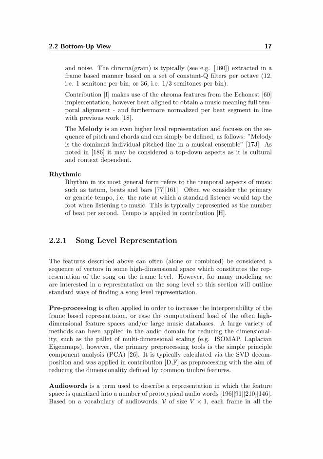
2.2 Bottom-Up View 17
and noise. The chroma(gram) is typically (see e.g. [160]) extracted in aframe based manner based on a set of constant-Q filters per octave (12,i.e. 1 semitone per bin, or 36, i.e. 1/3 semitones per bin).
Contribution [I] makes use of the chroma features from the Echonest [60]implementation, however beat aligned to obtain a music meaning full tem-poral alignment - and furthermore normalized per beat segment in linewith previous work [18].
The Melody is an even higher level representation and focuses on the se-quence of pitch and chords and can simply be defined, as follows: ”Melodyis the dominant individual pitched line in a musical ensemble” [173]. Asnoted in [186] it may be considered a top-down aspects as it is culturaland context dependent.
RhythmicRhythm in its most general form refers to the temporal aspects of musicsuch as tatum, beats and bars [77][161]. Often we consider the primaryor generic tempo, i.e. the rate at which a standard listener would tap thefoot when listening to music. This is typically represented as the numberof beat per second. Tempo is applied in contribution [H].
2.2.1 Song Level Representation
The features described above can often (alone or combined) be considered asequence of vectors in some high-dimensional space which constitutes the rep-resentation of the song on the frame level. However, for many modeling weare interested in a representation on the song level so this section will outlinestandard ways of finding a song level representation.
Pre-processing is often applied in order to increase the interpretability of theframe based representtaion, or ease the computational load of the often high-dimensional feature spaces and/or large music databases. A large variety ofmethods can been applied in the audio domain for reducing the dimensional-ity, such as the pallet of multi-dimensional scaling (e.g. ISOMAP, LaplacianEigenmaps), however, the primary preprocessing tools is the simple principlecomponent analysis (PCA) [26]. It is typically calculated via the SVD decom-position and was applied in contribution [D,F] as preprocessing with the aim ofreducing the dimensionality defined by common timbre features.
Audiowords is a term used to describe a representation in which the featurespace is quantized into a number of prototypical audio words [196][91][210][146].Based on a vocabulary of audiowords, V of size V × 1, each frame in all the

18 Computational Representation of Music
audio songs can be assigned in a hard manner to a single audioword corre-sponding to the well-known technique of vector quantization (VQ). In a song,s, a particular word from the vocabulary of audiowords at position/frame iis denoted, ws,i, and the sequence becomes a vector of integer indexes, i.e.,
ws =[ws,1, ws,1, .., wsNs
]>. There are various strategies towards finding the
audiowords, and possibly the simplest is to apply a K-means algorithm [26]with a fixed number of K centers. Obviously any (spectral) clustering (hard orsoft), sensible decomposition (such as normalized matrix factorization) may beused to define the audio words (followed by hard assignment). In contribution[H] an online version of the K-means algorithm [106] was applied for scalabilityon the Million Song Dataset (MSD) [20].
Temporal considerations: Many of the bottom-up features outlined above -or their low-rank and vector quantized version - are typically based on the framebased analysis as outlined in Fig. 2.1, thus a sequence of vectors. The obvioustemporal aspect of audio has spurred a vast amount of work in representing andmodelling temporal. The approaches can roughly be categorized as follows:
Temporal Independence - bag-of-frames In the simplest possible - but widelyapplied approach - we assume that the frames are independent and obtaina so called bag-of-frames approach.
• Mean-Variance / Gaussian:A simple statistical representation of a set of vectors in a song, s,is the multi-dimensional mean vector, µs, and variance, σs, of themulti-dimensional observations. This can naturally be generalized toa probability, and given the often continuous features, the naturaldistribution is a standard Gaussian, i.e.the representation for a song,s is simply
p (x|θs) = N (x|µs,Σs)
where θs = {µs,Σs}. µs is the mean of the distribution and Σs isthe covariance matrix. While seemingly simple, this representationhas been argued to be rich enough [143], at least for classificationpurposes.
• Gaussian Mixture ModelThe single Gaussian representation is possibly enough in many situa-tion and systems [143], however another popular approach is to gener-alize the Gaussian representation to a mixture of individual Gaussianusing the Gaussian Mixture Model (GMM) to define a considerablymore complex density, i.e.,
p (x|θs) =
Z∑
z=1
p (z) p(x|θ(z)
s
)=
Z∑
z=1
p (z)N(x|µ(z)
s ,Σ(z)s
)

2.2 Bottom-Up View 19
where θs ={θ(z)s
}z=1:Z
and θ(z)s =
{µ
(z)s ,Σ
(z)s
}. The mixing pro-
portions, p(z), further has the constraint p (z) ∈ [0, 1] andZ∑z=1
p (z) =
1. The model is typically estimated using standard expectation max-imization algorithm [26]. Determining the model complexity is gen-erally a tricky matter and may be performed using the Akiies Infor-mation Criterion (AIC) or the Bayesian Information Criterion (BIC)[190][26], penalizing the resulting log-likelihood with a complexityterm depending on the number of free parameters in the model.
• Histograms for audio word models:In case the audio feature space has been quantized into audio words,we may represent the song as a sequence of the audiowords. However,in the bag-of-frames assumption the order does not matter and thesong may be represented counting the number of occurrences of theaudiowords in the vocabulary. This may be expressed as counts of(audio)words in a given song, n (ws = v) where v is the index into thevocabulary, V. This results in a bag-of-(audio)words representationwhere each song is represented by a x ∈ NV vector of counts xs =[n (ws = 1) , n (ws = 2) , ..., n (ws = V )]
>
This bag-of-frames representation obviously requires less estimationand computation than the GMM, and was used for scalability rea-sons in contribution [H] on the MSD. In some settings, the vector ofcounts may be represented as a probability mass function, i.e., as adistribution over all words for a given song. This is implicitly donein for example [7] for a topic model, and [146] for use in a kernelmethod.
Temporal Integration A number of approaches has been suggested aimingto integrate the low-level short time features into a longer frame in effectintegrating temporal information into new features and representationswhich may then be applied in a algorithm. This approach can often bedivided into a number of categories depending on what temporal level ansubsequent algorithm makes its decision
• Early: Integration of information from each analysis frame can in thesimplest form be conducted by stacking individual frames. A moreadvanced approach is the multi-variate auto-regression (AR) mod-elling across multiple analysis frames, resulting in intermediate levelframes with for example AR coefficients (see [150] for an overview).
• Late: Another formally not a bottom-up approach is to make deci-sions for each analysis frame and subsequently make a single jointdecision based for example on majority voting [150].

20 Computational Representation of Music
Temporal Modelling The most elaborate approach to include temporal infor-mation is a ’real’ modelling of the temporal dynamics which can be doneusing for example hidden Markov models, or the more suitable dynamictexture mixture model [12][11].
The song level representation applied in the contributions is typically theGaussian Mixture Model. There exist many proposals and evaluations [98][9] ofvarious measures of unsupervised similarity measures between densities. Basedon a single feature vector - and possibly the mean of the Gaussian - simpledistance measure such as the Euclidian, cosine or Mahanalobis distance may beapplied to define similarity between audio. More elaborate and popular sim-ilarity measures include the (Symmetrized) Kullback-Leibler (KL) divergencebetween densities. This can be computed in closed form with single compo-nents, however must be evaluated by stochastic simulation for general mixtures.The Earth Mover distance [134] is an approach to get around the KL divergencesproblem with more than one component. The Hellinger distance [98] is an alter-native measure between distributions, which can be generalized to mixtures inanalytical form [97]. A particular intriguing approach is based on the Bayesian,non-parametric Hierarchal Dirichlet Process approach [90] effectively encodingall songs with a a-prior assumption of infinite number of Gaussians common toall songs. Each song is then coded as a mixture of these common Gaussians,and similarity is given by the mixing proportions corresponding to p(z).
Tasks which rely on such music representations and similarities, include purelybottom-up driven tasks like content based recommendation. However, for thespecific task of mapping to some label, e.g, genre, we often turn to supervisedmachine learning algorithms (including the ones considered in Chapter 3), whichare based directly or indirectly on metrics or similarity functions. Well-knownalgorithm include K-nearest neighbor [26] and kernel machines [197][26] suchas the Support Vector Machine (SVM), widely popular in the MIR community.There is in general no requirements for the similarity function used in the K-nearest neighbor algorithm, however any algorithm based on kernels, formallyrequire the kernel to be positive semi definite (PSD) (disregarding the notion ofconditional PSD kernels). Provided that the defined similarity is a valid metric(e.g. [84]) it may directly be converted into a valid kernel function [81] 2.
The kernel based algorithms provide flexible alternatives to vector space algo-rithms, since the only requirement is a valid kernel (perhaps derived from a validmetric), which can be formulated for many objects such as strings, text and dis-tributions. In particular, contribution [D] makes use of the probability productkernel (PPK) [97] (described in more detail in Sec.3) for defining correlationbetween the bottom-up audio features in terms of each songs density given by
2As considered in the co-authored paper [4]
2.3 Top-Down View 21
the GMM. The PPK has gained some attention in the MIR community andhas been applied in [152][150][14] with GMM and MAR, and most recently in[146] using a histogram representation. Furthermore, contribution [F,D] utilizesthe PPK based on the Gaussian Mixture Model representation. Alternatives inthe MIR community includes the symmetric Kullback-Leibler divergence basedkernel (see e.g [151]), which is formally not a PSD kernel. And the much sim-pler option of applying a squared exponential on a vectorized version of theGaussian representation (or the mixture) is often a simpler alternative. Such arepresentation is applied in contribution [E].
2.3 Top-Down View
The bottom-up view as defined by the content based analysis and metadata, hasbeen a primary driver of music similarity in the early years. However, in recentyears many successful music studies and services are based not on the contentitself, but on the ratings and opinions of users, in a so called collaborative filtersetups. This is the text book example of a purely top-down based system, wherethe users expressed views defines the possibly subjective similarity between mu-sic songs.
Such collaborative filters are certainly not the only form of user generated datasuitable for including in a top-down view of music and audio systems. A numberof such aspects (and related datasets) has been considering in the music infor-mation retrieval and analysis community), and we here provide an overview ofthe approaches and relevant studies.
Preference - ratings and rankingsSubjective audio and music preference is a major aspect in recommenda-tion and understanding of user representation and needs. Such preferenceratings is the basis of collaborate filtering systems (see e.g. [43] for ageneral overview) and has been investigated in numerous studies such as[42].
Collaborative filters usually suffers from very sparse data and have inthe MIR field been found to be biased by popular artists and popularityin general [43]. Another approach is a fully personalized system whichwas considered in contribution [D], where we proposed and investigateda paradigm, where users compare two music songs to elicit their musicpreference based on partial rankings of the music objects.
Audio preference was also considered in contribution [I], which attemptsto efficiently eliciting the preference in a music reproduction system where

22 Computational Representation of Music
the music signal is altered by a linear filter operation parameterized bysystem settings. The system task is to optimize the system parametersbased on a internal representation of the users preference.
Listening patternsListening patterns of users is an indirect preference rating method, wherethe frequency is a representative of preference. This is, however, prone topopularity as outlined in [43]. The million song dataset and the associatedTasteProfile dataset [2] - with more than one million users and more than48 million entries - offers the possibility of evaluating the usefulness oflistening patters for preference learning and recommendation.
Music emotion - expressed and inducedThat music has an emotional effect on humans is hardly a surprise andprobably one of the reason why music is such an important part of themodern life. Naturally, audio and music systems should take this impor-tant aspects into consideration, and in doing so, it is custom to differentiatebetween the expressed emotion and the induced emotions of the music.
Expressed emotions of music is the objective emotional expression themusic is believed to carry, i.e., it can be seen as the expression the com-poser is aiming to express [104]. Aimed to be an objective evaluation ofthe emotion which the music expresses; it is still influenced by the culturalbackground of the listeners [89][103]. The induced emotions refer to theaffect that the music has on the listener personally, i.e., highly depen-dent on internal representation (memories, experience etc) and context.Whether the distinction between expressed and induced emotion is fea-sible is certainly an issues [183][104], however not often discussed in theMIR community where the focus has been on the expressed emotion, thus,disregarding the affect the music has on the individual and focusing onthe (homogeneous) population used to examine it.
The experimental setup typically applied for examining the expressed emo-tion are categorical approaches [88] or dimensional approaches [184]. Thedimensional approach is the most applied in the MIR field [108], andthe preferred dimensions are arousal and valance denote the AV space.Valance spans a range from highly positive (happy) to highly negative(sad), whereas arousal ranges from calm/passive to excited/active [184].
From an application point of view, the aim is to model and predict theemotional expression in the AV space based on the bottom-up featureswhich can then be used in recommendation and retrieval systems. Anumber of approaches has been proposed in the MIR community (see [108]for a review). These are mainly based on so-called direct scaling methodsin which users are asked to assign a single absolute value on the AV scale,representing the emotion expressed by a particular piece of music. Thisis often highly susceptible to the users lack of understanding of the scale

2.3 Top-Down View 23
[140], due to the complex concepts of arousal and valance. This is inaddition with the cognitive difficult in separating the expressed emotionfrom the induced.
Contribution [E,F] consider the task of predicting the (expressed) emotionof music based on pairwise comparisons between individual songs in the AVspace, which is an alternative but more robust experimental paradigm thanabsolute rating. It has not yet fully been explored in the MIR community,although previously considered in [237].
Induced emotion is highly personal and even context dependent and hasseemingly not been investigated within the MIR field, possibly due tothe experimental difficulties in obtaining robust ratings and representa-tions [104]. It is, however, crucial to include such knowledge into trulypersonal systems where individuals are affected differently by the music.This personal aspect should optimally be elicited and represented by agiven system.
Annotation - categories and tagsCategorization of music, such as genre [68] is often a result of culturalunderstanding and grouping of music [52], and is therefore considered atop-down aspect in this context. The task of classifying music into genrebased on bottom-up features has been a defining task of MIR in manyyears (see [209] for a comprehensive review).
Fixed vocabulary based on a certain taxonomy/ontology, is a simpleform of tagging where genre based annotation can be seen as a specialcase. However, while genre is typically considered unique and exclusive,the general annotation setting allows multiple annotations per objects (andpossibly users). Examples of such fixed annotations in include [221] wherethe vocabulary is based on the CAL500 vocabulary [39], and a recentproposal of an ontology for music annotation [181].
Open vocabularies also known as a folksonomies, provides a setting,where the annotation themselves is the result of a conscious decision tofreely express the individual user representation towards an object or sys-tem result (see [118] for a general review). Thus, users are allowed toenter free text or even sentences expressing their view. A number of re-search and real-world datasets has been collection in the MIR field, in-cluding Magnatagatune [120], MajorMinor [142], last.fm [1] and CAL500[39]. Descriptive studies of open vocabulary annotations, include [125] us-ing probabilistic latent semantic analysis (pLSA), finding clear semanticpatterns. Similarly [72] uses open vocabulary tags from last.fm to evaluatethe similarity between artists also based on last.fm. [203] examines thealignment between genre and tags based on a fixed expert vocabulary andlast.fm. Prediction of these tags from e.g. the audio features is a commontask in MIR (e.g. [155][19][91]), often motivated from a recommendation

24 Computational Representation of Music
and retrieval point of view [43] in which the tagging induces a particulartop-down similarity.
Contribution [I] considers open vocabulary tags based on last.fm dataset.This is combined with the bottom-up view to show alignment betweenrepresentations and tags in a descriptive fashion.
Music similarity - explicit and implicitExplicit ratings of similarity of music objects is not a common approach inthe MIR community, but has gained some momentum with the MagnaTa-gAtune dataset [120]. Various approaches [207][234][235] been applied tolearn the similarity based on the odd-one-out experimental paradigm, i.e.,selecting the object which is most dissimilar to the two others 3. A sim-ilar approach was formulated in [62] considering ground truth for artistsimilarity.
Other approaches to similarity include explicit relevance feedback, whereusers indicate relevance of the returned search result. This as for exam-ple been proposed in [110] in which the user’s query is altered based onindicated relevance, and in [45] reweighing feature dimensions based onindicated relevance of search results.
The direct scaling of similarity is conjectured to be an important modellingaspect in future systems, since it provides a direct way to manipulatecomputational representations by expressed distances, or by e.g. odd-one-out paradigms [120], possibly in an interactive learning process.
Implicit ratings based on the general techniques of (implicit) relevancefeedback [10] amounts to observing the behavior of the user in relation toa system output, e.g., click-through behavior of music search. Such feed-back implicitly defines similarity between query and objects. Examples ofsuch ideas has been proposed in for example [174] examining the skippingbehavior in recommended music playlists .
Common knowledge and Web resourcesAn particular aspect of the top-down view is common knowledge, i.e.knowledge which has been collectively agreed upon such as encyclopediasand reference works. This covers some of the annotation aspects previouslymentioned, at least to some degree. Wikipedia, for example, contains adetailed description of genre and other music related aspects useable asgeneral top-down information. Such an approach was for example investi-gated in [157] examining content and links in Wikipedia’s music universe -and recently in [204], anchoring the patters found in an analysis of last.fmusing Wikipedia’s music universe. Other online sources of information are
3The framework presented in Sec. 3 can be used to model this dataset in a probabilisticmanner unlike e.g. [235]

2.4 Joining Views 25
Twitter and similar services, which can provide top-down information re-garding the objects, such as the preference covered above. It can furthergive detailed insight into the users general context, including activities andstate of mind. Online social network such as Facebook and Twitter canbe a potential source of top-down and contextual information in collab-orative filtering settings, inline with the friend-of-a-friend (FOAF) ideaspresented in [42][43].
2.4 Joining Views
The tasks related to the various views typically focuses on mapping from abottom-up view to the top-down view in order to utilize the bottom-up (or con-tent based) analysis to enrich the users in a given system. Such task includesupervised auto-tagging [91][19], unsupervised similarity computation based onbottom-up similarity (e.g. [98]), supervised genre classification based on bottom-up features [209] and unsupervised (with auxiliary task) tag analysis [126]. Here,the focus is on the combination of views - or modalities. Modern music organi-zation systems and services, such as last.fm, typically have access to (multiple)bottom-up and top-down views, but a major challenge is to utilize either, orboth, to create an effective computational representation, which aligns well withthe (individual) user representation as argued in Chapter 1.
In recent years, this has spurred a large interest in multimodal integration ofviews - or modalities - for a number of tasks typically within retrial and recom-mendation domain. Particular focus has been on hybrid recommendation basedon collaborative filtering and content based features (e.g. [240]), discriminativesemantic retrieval by combining kernels [14] and playlist generation by apply-ing a hyper-graph approach, using many different modalities and learning theweight of each modality discriminatively [148]. Recently [149] applied multi-way canonical correlations analysis (CCA) based on bottom-up audio features,lyrics and tags to analyze emotional aspects of music based on the Million SongDataset [20].
A further advantage of including multiple bottom-up and top-down views in asingle suitable model, is the possibility for a the single model to solve multipletasks previously covered by many different algorithms. The work in [229] isa proposal for such a multi-task system in the MIR field. Contribution [H] isan proposal of a probabilistic and generative approach towards such a systemproviding a relatively simple probabilistic approach. It integrates the bottom-up view (the audio features), the meta-data (lyrics) and a top-down view basedon open vocabulary tags.
26 Computational Representation of Music
2.4.1 Example: Multimodal Integration
A concrete example where multimodal integration is an natural and often re-quired approach is large scale music modelling which has become possible dueto the release large linked datasets such as the million song dataset (MSD). Incontribution [H] a setup is proposed which considers a number of the alreadyoutlined views or modalities, in particular
AudioThe audio content is represented by bottom-up analysis. In particularfour fundamental aspects covering all of the musical aspects outlined inSec.2.2. I.e. timbre (x(timbre) ∈ R12), rhythmic (x(tempo) ∈ R), harmonic(x(chroma) ∈ [0, 1]12) and loudness (x(loudness) ∈ R1). The features areextracted by Echonest and already available in the MSD, however, thesetup aligns the event based segment to the beats of the song in orderto obtain music meaningful analysis frames (songs with no defined beatmaintain the segment based analysis frames).
The million songs in the MSD poses a computational problem due to themere size of the dataset. Contribution [H], therefore, takes the audiowordapproach outlined in 2.2 in which the common feature space is vectorquantized (VQ) and frames in each song assigned to a single audioword.
The song level representation is obtained by assuming that the frames areindependent, i.e., no temporal integration is performed in [H]. This meansthat each of the million songs is represented by a count of individualaudiowords. In contribution [H] the combined audio vocabulary is of sizeV (tags) = 2112 audio words.
LyricsThe textual lyrics of a song is another fundamental modality, which isintegrated in the setup. The lyric representation is in a bag-of-(lyric)-words similar to the audiowords. The lyric vocabulary is of size V lyric =5000 ( available in the MSD).
TagsThe user generated top-down is based on open vocabulary tags originatingfrom last.fm. They are represented as a bag-of-words of size V (tags) =20.000 including the most popular tags out of more than 500.000 uniquetags.
EvaluationThe setup uses other top-down information which is not included in therepresentation itself. These are genre (15 categories/classes) and style
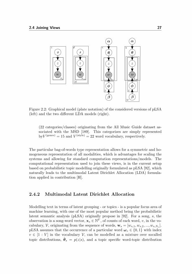
2.4 Joining Views 27
Figure 2.2: Graphical model (plate notation) of the considered versions of pLSA(left) and the two different LDA models (right).
(22 categories/classes) originating from the All Music Guide dataset as-sociated with the MSD [189]. This categorizes are simply representedbyV (genre) = 15 and V (style) = 22 word vocabulary, respectively.
The particular bag-of-words type representation allows for a symmetric and ho-mogeneous representation of all modalities, which is advantages for scaling thesystems and allowing for standard computation representations/models. Thecomputational representation used to join these views, is in the current setupbased on probabilistic topic modelling originally formulated as pLSA [92], whichnaturally leads to the multimodal Latent Dirichlet Allocation (LDA) formula-tion applied in contribution [H].
2.4.2 Multimodal Latent Dirichlet Allocation
Modelling text in terms of latent grouping - or topics - is a popular focus area ofmachine learning, with one of the most popular method being the probabilisticlatent semantic analysis (pLSA) originally propose in [92]. For a song, s, theobservation is a song-word vector, xs ∈ NV , of counts of each word, v, in the vo-cabulary, V, originating from the sequence of words, ws = [ws,1, ws,2, ..., ws,Ns
].pLSA assumes that the occurrence of a particular word ωv ∈ {0, 1} with indexv ∈ [1 : V ] in the vocabulary V, can be modelled as a mixture over socalled
topic distributions, θs = p(z|s), and a topic specific word-topic distribution

28 Computational Representation of Music
φz = p(ωv=[1:V ]|z
)Hence, the probability for observing a vocabulary word in
a particular song, s, is given by p (ωv = 1|s) =∑Zz=1 p (ωv|z) p (z|s).
Hence, the pLSA model defines Z latent groups of words also referred to astopics. The graphical model of this simple mixture is shown in Fig. 2.2, whichshows the underlying generative story (effectively resulting in the mixture),that for all words with position i in a particular song a topic zs,i is drawn fromp(z|s) after which a word ws,i ∈ [1 : V ] is drawn from p(ω|z). We of course
require∑Vv=1 p (ωv|z) = 1 and
∑Zz=1 p (z|s) = 1, such that the draw is from a
Categorical distributions.
Multiple modalities with each their vocabulary, V(m), is modelled by assumingconditional independence between modalities,i.e.,
p(ω(1)v ,ω(2)
v , ...,ω(M)v |s
)=∑Z
z=1p (z|s)
∏M
m=1p(ω(m)v |z
)(2.1)
This results in a modality specific word-topic distribution p(ω(m)|z). Estimationof the model parameters, i.e. the point estimates of all the vectors denotedθs = p(z|s) and φz = p(ω|z), is done by observing that given a song and amodality, words are generated independently. Thus, the total data likelihood
for a sequence of observed words, w(m)s , in a modality is simply a function of
the number of counts of each word indexed by v, thus adhering to the bag-of-words representation. The likelihood of a corpus with counts, X, consisting ofS songs with M modalities, is typically performed using maximum likelihood
based on the total data log likelihood given as, p (X) =S∏s
M∏mp(x
(m)s
)due to
the conditional independence between word and between modalities. Hence, thelog likelihood becomes,
logL (θ; X) =
S∑
s
M∑
m
Xs,v.m log
(Z∑
z
p(ω(m)|z
)p (z|s)
)
where Xs,v.m = n(w(m)s = v) denotes the count of the modality specific vo-
cabulary words in each song, i.e. the bag-of-words representation. θ denotesall the model parameters. The likelihood can be maximized by standard toolssuch as the Expectation Maximization (EM) algorithm easily derived, also forthe multimodal version, and suggested in the original pLSA formulation [92].Another, but equivalent approach is based on the easy recognizable relation toNon Negative Matrix factorization (NMF) [58] applied for music analysis in forexample [7][157]4. The equivalence is based on the direct use of Kullback-Leiblerdivergence as the NMF objective (as opposed to the ’indirect’ use in the EMcase) to derive the multiplicative updates [123][58].
4Although with the least-squares objectives and an appropriate normalization

2.4 Joining Views 29
Contribution [H] extends the popular (multimodal) pLSA model by consideringthe Bayesian version for music modelling, namely the Latent Dirichlet Allocation(LDA). LDA was introduced in [29] with the aim to provide a valid generativemodel for text documents/songs, which is formally lacking in the pLSA model[29], since there is no way of generating a new document, i.e. obtaining a topicdistribution for it.
The LDA model accomplishes this by considering the topic distribution, θs,a real random variable and not a fixed parameter given the song, as in thepLSA model. With the topic distribution being a random variable, θs, LDAspecifically places a common Dirichlet prior over it. The generative story nowholds, since a new document may be generated by drawing a topic distributionfrom this common prior. Now it is possible draw a particular topic , zs,i, fora word at position i in song s. Secondly, in the smoothed extension of LDA,a Dirichlet prior is also introduced over the word-topic distribution, such thatwith a particular topic zs,i, a word at position i is draw from p(ω|φzs,i), acategorial distrbution. The graphical model for the smoothed LDA model isshown in Fig. 2.2.
The multimodal LDA, mmLDA, is a straightforward extension of standard LDAtopic model [29], as shown in Fig. 2.2. The model is easily understood by theway it generates a new song by the different modalities. The generative process,which defines the model, is given by
• For each topic z ∈ [1;Z] in each modality m ∈ [1;M ]
Draw φ(m)z ∼ Dirichlet(β(m)).
This is the zth topic’s distribution over vocabulary Vm in modality m.
• For each song s ∈ [1;S]
– Draw θs ∼ Dirichlet(α).This is the sth song’s distribution over the topics [1;Z].
– For each modality m ∈ [1;M ]
∗ For each word position in the song i ∈ [1;Nsm]
· Draw a specific topic z(m)s,i ∼ Categorical(θs)
· Draw a word w(m)s,i ∼ Categorical(φ
(m)
z(m))
The important aspect to notice is that each song has a particular distributionover topics drawn from the common Dirichlet prior, and that each modality hasits own word-topic distribution. The joint probability of observations, ws, andthe latent variables, zs, for each song and modality in the full corpus W and Z
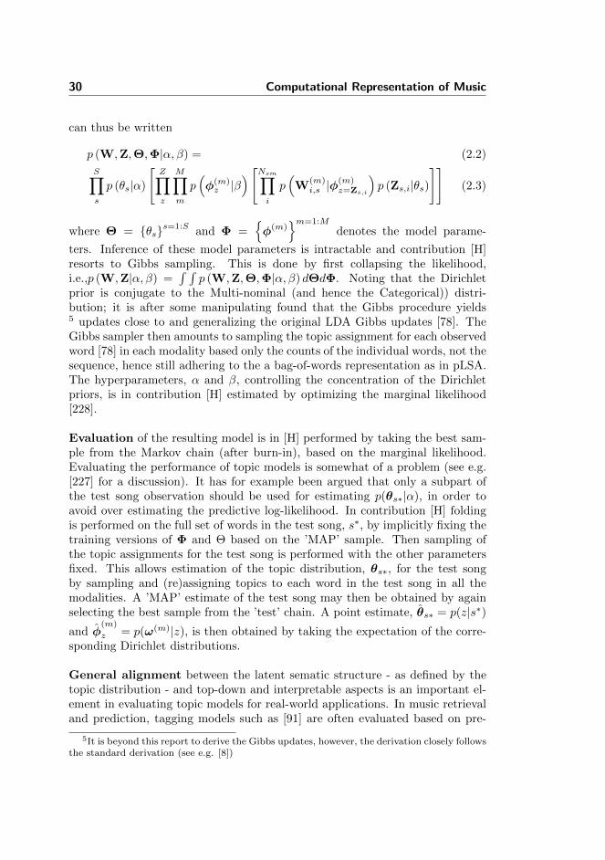
30 Computational Representation of Music
can thus be written
p (W,Z,Θ,Φ|α, β) = (2.2)
S∏
s
p (θs|α)
[Z∏
z
M∏
m
p(φ(m)z |β
)[Nsm∏
i
p(W
(m)i,s |φ
(m)z=Zs,i
)p (Zs,i|θs)
]](2.3)
where Θ = {θs}s=1:Sand Φ =
{φ(m)
}m=1:M
denotes the model parame-
ters. Inference of these model parameters is intractable and contribution [H]resorts to Gibbs sampling. This is done by first collapsing the likelihood,i.e.,p (W,Z|α, β) =
∫ ∫p (W,Z,Θ,Φ|α, β) dΘdΦ. Noting that the Dirichlet
prior is conjugate to the Multi-nominal (and hence the Categorical)) distri-bution; it is after some manipulating found that the Gibbs procedure yields5 updates close to and generalizing the original LDA Gibbs updates [78]. TheGibbs sampler then amounts to sampling the topic assignment for each observedword [78] in each modality based only the counts of the individual words, not thesequence, hence still adhering to the a bag-of-words representation as in pLSA.The hyperparameters, α and β, controlling the concentration of the Dirichletpriors, is in contribution [H] estimated by optimizing the marginal likelihood[228].
Evaluation of the resulting model is in [H] performed by taking the best sam-ple from the Markov chain (after burn-in), based on the marginal likelihood.Evaluating the performance of topic models is somewhat of a problem (see e.g.[227] for a discussion). It has for example been argued that only a subpart ofthe test song observation should be used for estimating p(θs∗|α), in order toavoid over estimating the predictive log-likelihood. In contribution [H] foldingis performed on the full set of words in the test song, s∗, by implicitly fixing thetraining versions of Φ and Θ based on the ’MAP’ sample. Then sampling ofthe topic assignments for the test song is performed with the other parametersfixed. This allows estimation of the topic distribution, θs∗, for the test songby sampling and (re)assigning topics to each word in the test song in all themodalities. A ’MAP’ estimate of the test song may then be obtained by againselecting the best sample from the ’test’ chain. A point estimate, θs∗ = p(z|s∗)and φ
(m)
z = p(ω(m)|z), is then obtained by taking the expectation of the corre-sponding Dirichlet distributions.
General alignment between the latent sematic structure - as defined by thetopic distribution - and top-down and interpretable aspects is an important el-ement in evaluating topic models for real-world applications. In music retrievaland prediction, tagging models such as [91] are often evaluated based on pre-
5It is beyond this report to derive the Gibbs updates, however, the derivation closely followsthe standard derivation (see e.g. [8])

2.4 Joining Views 31
cision/recall and mean average precision [144], which focuses on the number ofcorrectly retried tags or possibly songs based on query tags. In contribution [H],a different approach is suggested which aims at evaluating the general alignmentof the computational representation with a given (not included) view/modality,m∗. The suggested approach makes use of the mutual information between thecomputational representation given by the LDA model, in particular p(z|s∗)and p(ω(m)|z). Given an auxiliary task/modality, m∗, we calculate the mutualinformation between individual words ωm∗v ∈ {0, 1}, indicating the occurrenceof a particular word in the test modality or not, and the topic indicator variablez ∈ [1 : Z]. Thus,
MI(ω(m∗)v , z|s∗
)= KL
(p(ω(m∗)v , z|s
)||p(ω(m∗)v |s
)p (z|s)
)(2.4)
=∑
ω∈{0,1}
Z∑
z=1
p(ω(m∗)v |z
)p (z|s∗) log
p(ω
(m∗)v |z
)
∑z′p(ω
(m∗)v |z′
)p (z′|s∗)
(2.5)
The probability of the particular word not occurring, i.e., ωm∗
v = 0, is simply
p(ω
(m∗)v = 0, z|s∗
)= 1− p
(ω
(m∗)v = 1, z|s∗
).
The mutual information is normalized and averaged over all songs, thus the final
measure of alignment is the average mutual information, avgNMI(ω(m∗)v ), for
each test word ω(m∗)v .
This relatively simple approach supports evaluating the alinement of a represen-tation with auxiliary top-down views by ranking the auxiliary words by avgNMI,thus finding the test words which are best explained by the representation. Thisis for example analysed in [H], where the alignment of a multimodal music rep-resentation (based on bottom-up features) is evaluated against the top-downview (as represented by open vocabulary tags).
2.4.3 Discussion and Extensions
The joint representation relies on information originating from the top-downview, i.e., data generated from users expressing their conscious or unconsciousview on the object or the system output. This is usually a time consuming andexpensive process to obtain these user generated data, and does seldom provideany direct and obvious benefit to the users. An example includes the last.fmin which it is possible to tag each song, however the immediate gain in doingso is not apparent. However, the combined tagging space is presumable used
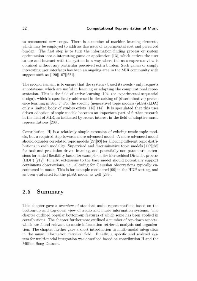
32 Computational Representation of Music
to recommend new songs. There is a number of machine learning elements,which may be employed to address this issue of experimental cost and perceivedburden. The first step is to turn the information finding process or systemoptimization into a interesting game or application [13], which entices the userto use and interact with the system in a way where the uses expresses view isobtained without any particular perceived extra burden. Such games or simplyinteresting user interfaces has been an ongoing area in the MIR community withsuggest such as [120][107][221].
The second element is to ensure that the system - based its needs - only requestsannotations, which are useful in learning or adapting the computational repre-sentation. This is the field of active learning [194] (or experimental sequentialdesign), which is specifically addressed in the setting of (discriminative) prefer-ence learning in Sec. 3. For the specific (generative) topic models (pLSA/LDA)only a limited body of studies exists [115][114]. It is speculated that this userdriven adaption of topic models becomes an important part of further researchin the field of MIR, as indicated by recent interest in the field of adaptive musicrepresentations [208].
Contribution [H] is a relatively simple extension of existing music topic mod-els, but a required step towards more advanced model. A more advanced modelshould consider correlated topic models [27][63] for allowing different topic distri-butions in each modality. Supervised and discriminative topic models [117][28]for task and prediction driven learning, and potentially non-parametric exten-sions for added flexibility based for example on the hierarchical Dirichlet process(HDP) [212]. Finally, extensions to the base model should potentially supportcontinuous observations, i.e., allowing for Gaussian observations typically en-countered in music. This is for example considered [90] in the HDP setting, andas been evaluated for the pLSA model as well [239].
2.5 Summary
This chapter gave a overview of standard audio representations based on thebottom-up and top-down view of audio and music information systems. Thechapter outlined popular bottom-up features of which some has been applied incontributions. The chapter furthermore outlined a number of top-down aspects,which are found relevant to music information retrieval, analysis and organiza-tion. The chapter further gave a short introduction to multi-modal integrationin the music information retrieval field. Finally, a specific and realized sys-tem for multi-modal integration was described based on contribution H and theMillion Song Dataset.

Chapter 3
Preference Learning withGaussian Processes
Ranking and rating of objects by human subjects is a common source of top-down information in many multimedia systems such as online movie recom-mendation services [166], book stores [6] and music services [1]. A noticeablecharacteristic of these examples is the human and cognitive implication since allexamples depends on some subjective understanding of the objects and whatrelevance, similarity and preference is in relation to the those objects. We willgenerally consider such ranking and rating scenarios under the common term ofpreference learning, however the principle has applications much beyond pref-erence learning and modelling.
The response is given by subjects who are asked to convey some notion ofpreference in the form a response, y, towards one or more objects from the(choice1) set C = {xi|i = 1...C, C <∞,x ∈ X}, where X is a set of N inputinstances, X = {xi|i = 1...N,x ∈ X}. This can for example be a ranking ofmultiple objects, a rating of similarity between two objects, or directly assigninga noisy absolute value to the object. The resulting set of K such observationsis denoted Y = {(yk; Ck) |k = 1...K, y ∈ Y}2.
1Only called a choice set in case of discrete choices2The notation (yk; Ck) is used to indicate that yk is dependent on the choice set, not part
of the set as such.
34 Preference Learning with Gaussian Processes
This response- or observation types, can along with many others, be dividedinto two fundamentally different groups, namely
• Relative (or indirect scaling [16]) Comparing (a finite set) of ob-jects and ranking them in order (discrete choice / permutation model, e.g.[220][17]) or assigning value to the similarity between them. Dependingon the setting, yk ∈ {−1, 1} yk ∈ [1 : C], yk ∈ P where P denotes allpossible permutations of the C objects, e.g. yk = {4, 1, 3, 2}.
• Absolute (or direct scaling [16]) Assigning an absolute value to eachobject (regression model), e.g. yk ∈ R or yk ∈ [0, 1].
The main assumption is, regardless of the response type, that each object x ∈ Xhas a latent value f(x) and the response given by the subject is dependent onthese latent values, whether this being in terms of one value (the absolute case)or in terms of multiple values, e.g. difference or rations between values (relativecase).
The relative (or indirect) case typically calls for models based on discretechoice models in which either: a) one and an only one outcome is selected or b) aspecific permutation of C objects is chosen, indicating the ranking of the objects.Modelling such discrete choices was considered by Thurstone [216] in his seminalpaper ’The law of comparative judgement’, which lays the groundwork for theprobit choice model considered in Sec. 3.2, and the basic working principleof socalled Thurstonian models. Later Bradley and Terry [35] developed theBradley-Terry (BT) model, in effect a logit model for pairwise comparisons.Luce later extended this view with the Bradley Terry Luce (BTL) model [135]- or unordered multinomial/generalized logit - which laid the groundwork for’Luce’s axoim of choice’ and the specific incarnation of the logistic function aschoice model.
These discrete choice models can be extended to likelihood functions over per-mutations of objects, such as the Placett-Luce model originating from the BTLmodel [178], and a similar principle based on probit model [238], albeit the latterwith much more difficult estimation/inference than the Placett-Luce. An evenmore general view can be obtained by considering general exponential forms forpermutations such as the Mallow models [141], which is however not consideredhere.
A particular special case of discrete ranking models arises when only partialrankings are observed (C < N and typically C << N), and the focus in thischapter is mainly on the special case when only two objects are considered atthe time, i.e. y ∈ {−1, 1}. The resulting pairwise scenario results in a number
35
of paired observations where two different objects are ranked. Furthermore,the comparison between the two objects could potentially result in assigninga value to the difference between objects or degree of preference indicating forexample beliefs or confidence in the decision. This latter aspect is considered incontribution [C].
In direct scaling paradigms i.e. the absolute case the subject assigns an ab-solute value to each object, essentially calling for regression models. Typicallysuch ratings are given on a bounded or/and ordinal scale, in which case, aconsistent modelling framework requires specialized noise/likelihood models asconsidered in Sec. 3.2.
Modelling these specialized response types is a major questions. In order tonarrow down the possibilities, a number of properties is considered, often foundin multimedia objects and elsewhere in machine learning, namely
I) High dimensional features spaces
II) (Relatively) few labeled examples
III) Unknown - or varying - task complexity (linear/non-linear)
IV) Multiple and heterogeneous sources of information
V) Limited time for experimentation (a cause of the few labeled samples)
VI) Possibility to predict f(x∗) for unseen examples,x∗
The last aspect is not a must in a frequentist view using classical hypothesistests. However, with the system and machine learning applications in mind,this is a requirement and immediately calls for modelling the latent preferencevalues as a function. Aspect I-III calls for robust and flexible regression frame-works, and aspect IV calls for a flexible data representations. Aspect V callsfor the ability to express (at least predictive) uncertainty such that sequentialexperimental design becomes feasible.
With these aspects in mind, the choice of modelling framework has fallen onBayesian approach, and in particular a non-parametric versions based on Gaus-sian process priors on the function, f(·). In this Bayesian formulation, priorinformation can ensure robust and flexible modelling even given the adverseproperties listed above. The non-parametric nature, furthermore, allows forarbitrary flexibility in the underlying function only assuming some notion ofsmoothness .
In this Bayesian framework, it is only assumed that the likelihood function canbe parameterized by the function, f(·), and can be written in a factorized form
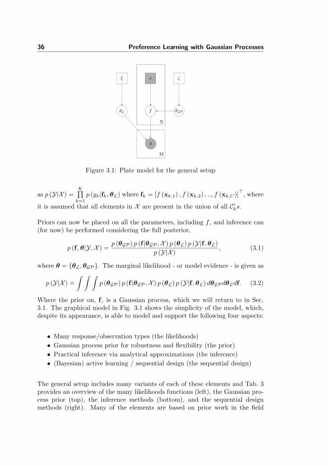
36 Preference Learning with Gaussian Processes
Figure 3.1: Plate model for the general setup
as p (Y|X ) =K∏k=1
p (yk|fk,θL) where fk = [f (xk,1) , f (xk,2) , .., f (xk,C)]>
, where
it is assumed that all elements in X are present in the union of all C′ks.
Priors can now be placed on all the parameters, including f , and inference can(for now) be performed considering the full posterior,
p (f ,θ|Y,X ) =p (θGP) p (f |θGP ,X ) p (θL) p (Y|f ,θL)
p (Y|X ), (3.1)
where θ = {θL,θGP}. The marginal likelihood - or model evidence - is given as
p (Y|X ) =
∫ ∫ ∫p (θGP) p (f |θGP ,X ) p (θL) p (Y|f ,θL) dθGPdθLdf . (3.2)
Where the prior on, f , is a Gaussian process, which we will return to in Sec.3.1. The graphical model in Fig. 3.1 shows the simplicity of the model, which,despite its appearance, is able to model and support the following four aspects:
• Many response/observation types (the likelihoods)
• Gaussian process prior for robustness and flexibility (the prior)
• Practical inference via analytical approximations (the inference)
• (Bayesian) active learning / sequential design (the sequential design)
The general setup includes many variants of each of these elements and Tab. 3provides an overview of the many likelihoods functions (left), the Gaussian pro-cess prior (top), the inference methods (bottom), and the sequential designmethods (right). Many of the elements are based on prior work in the field

3.1 Gaussian Processes 37
and some are merely included to provide a coherent and complete overview andtaxonomy, but not yet realized. Contributions [C],[G] and [D] can be seen asdevelopment steps towards the general setup, whereas contributions [E],[F] and[I] are direct applications of the realized setup.
Outline: The rest of this chapter aims to explain the elements of the overviewshown in 3 starting with a short review of Gaussian processes and a basicoverview of inference methods considered in Sec. 3.1. This is followed by anoverview in Sec. 3.2 of how and why Gaussian processes can/should be applied inranking and preference learning scenarios. Sec. 3.2 furthermore describes someof the contributes to the field, in particular new likelihood functions relevant forthe preference and ranking modelling. Sec. 3.3 provides a combined overviewof sequential design methods and sparse Gaussian processes - with focus onlearning and computational complexity for preference leaning and ranking.
3.1 Gaussian Processes
The modelling element differentiating the preset setup from other choice mod-elling frameworks such as generalized linear models (GLM) [220][36] is the par-ticular prior placed on the function values, f(x), namely the Gaussian process(GP). The Gaussian process is simply defined as: ’A collection of random vari-ables, any finite number of which have a (consistent) joint Gaussian distribu-tion’, [182]. It is here denoted, f ∼ GP
(m (x) , k (x, ·)θGP
).
The GP is defined by its mean function, E {f (x)} = m (x), and a covariancefunction k(x, ·|θGP) which - given the hyperparameters collected in θGP - de-fines the correlation between all individual variables, f(·). For a zero meanGP the correlation function is E {f(x)f(x′)} = k (x,x′)θGP . Since each ran-
dom variable, f(x), is correlated with another random variable f(x′) thoughthe covariance function, the function must necessarily have some smoothness.Furthermore, the ’nice’ marginalising and conditioning properties of the multi-variate Gaussian distribution makes the GP itself tractable. Fig. 3.2(a) showsthe graphical model for a GP.
By considering the function value of any input a random variable, the GP definesa prior over functions. From this prior, we may draw a finite number of functionvalues, f = [f(x1), f(x2), ..., f(xN )], and given the definition, we may continuedrawing function values for an infinite number of different inputs. Fig. 3.2(b)shows a number of functions drawn from an unconditioned GP. If observationabout f(x) the GP is simply defined by conditioning on these observations, Fig.3.2(c) shows functions drawn from a conditioned GP.

38 Preference Learning with Gaussian Processes
p(f|θ)
CovarinceInducedSparsity
HB*
/M
TK
ARD
/M
KL
PPK
/SSK
Pseudo
input
FIT
C/PIT
C(*)
Observatio
ns,p(y|f
)
Absolu
te
Contin
uous
Normal ** Random * Iterative
Sequentia
lD
esig
n
Student-t ** IVM * Acive Set
Warped . . . Methods
Beta Approx. * Pla
n
I:Com
putatio
n
Activ
eLearnin
g
Truncated G. Exact *
Discrete Probit/Logit
VOI
Greedy
EVOI
G’lized P/L * G(E)VOI
Ordinal P/L * CWS
Rela
tiv
e
Contin
ious Warped (*) PoI O
ptim
ize
II:
Task/Criterio
n
BetaEI
UCB
Truncated G. (*) THOMP
Discrete
Probit (Thurstone) Random Generaliz
atio
n
Logit (BT) Entropy
Ordinal P/L (*)
. . .BTL (G’lized logit)
Plackett-Luce
Exact
Lapla
ce
EP
(*)
MCM
C*
Inference,p(f, θ|D), p(y ∗ |D)
Table 3.1: General preference learning setup. Left: Likelihood func-tions Top: The GP prior specification Bottom: Inference methods Right:Sequential design elements. Note that elements form different directions(top/bottom/left/reight) are not exclusive, i.e., may in particular select bothsparsity by the pseudo input and the PPK covariance function. And the se-quential design in the active learning setting is required to select both a com-putational option and a task/criterior. Elements marked with ** has not beenimplemented in the setup but is often a part of other GP toolboxes such as theGPML toolbox [67]. Elements marked with * has not yet been implemented oronly partly (*), e.g. EP only exists for pairwise probit and absolute Beta/ trun-cated Gaussian (Truncated G.). Variational Bayes (VB) [167] has been omittedsince not considered in the thesis.
So the GP is nothing more than a prior over functions, indicating that the GPencompasses many different function classes, only assuming smoothness. Anylikelihood which can be parameterized by variables corresponding to particular
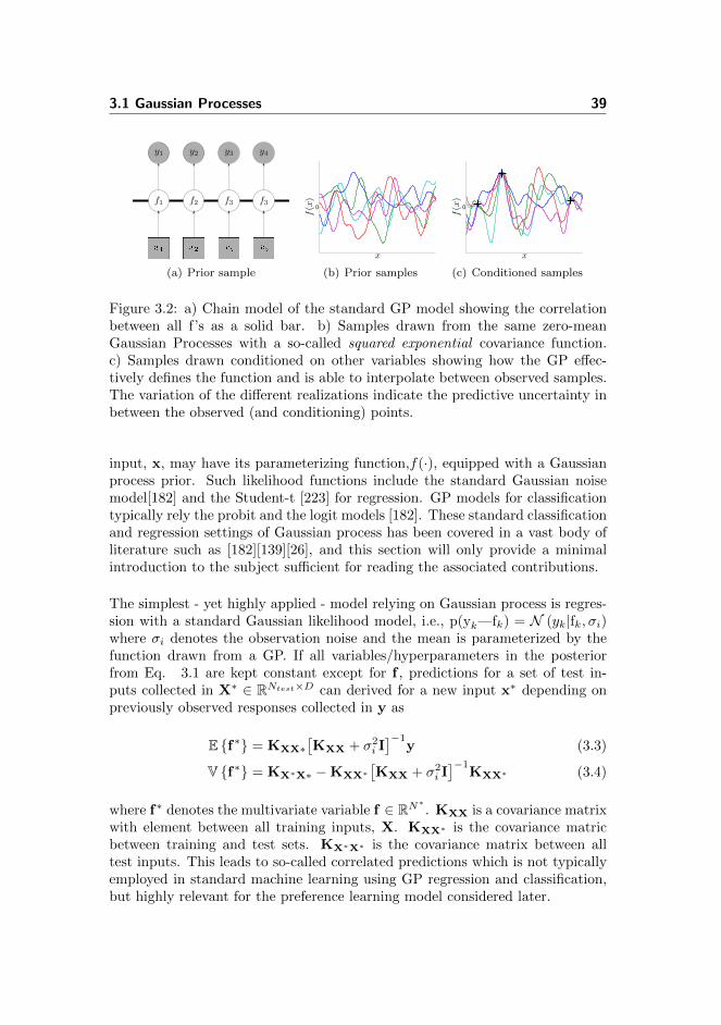
3.1 Gaussian Processes 39
(a) Prior sample
0
x
f(x)
(b) Prior samples
0
x
f(x)
(c) Conditioned samples
Figure 3.2: a) Chain model of the standard GP model showing the correlationbetween all f’s as a solid bar. b) Samples drawn from the same zero-meanGaussian Processes with a so-called squared exponential covariance function.c) Samples drawn conditioned on other variables showing how the GP effec-tively defines the function and is able to interpolate between observed samples.The variation of the different realizations indicate the predictive uncertainty inbetween the observed (and conditioning) points.
input, x, may have its parameterizing function,f(·), equipped with a Gaussianprocess prior. Such likelihood functions include the standard Gaussian noisemodel[182] and the Student-t [223] for regression. GP models for classificationtypically rely the probit and the logit models [182]. These standard classificationand regression settings of Gaussian process has been covered in a vast body ofliterature such as [182][139][26], and this section will only provide a minimalintroduction to the subject sufficient for reading the associated contributions.
The simplest - yet highly applied - model relying on Gaussian process is regres-sion with a standard Gaussian likelihood model, i.e., p(yk—fk) = N (yk|fk, σi)where σi denotes the observation noise and the mean is parameterized by thefunction drawn from a GP. If all variables/hyperparameters in the posteriorfrom Eq. 3.1 are kept constant except for f , predictions for a set of test in-puts collected in X∗ ∈ RNtest×D can derived for a new input x∗ depending onpreviously observed responses collected in y as
E {f∗} = KXX∗[KXX + σ2
i I]−1
y (3.3)
V {f∗} = KX∗X∗ −KXX∗[KXX + σ2
i I]−1
KXX∗ (3.4)
where f∗ denotes the multivariate variable f ∈ RN∗ . KXX is a covariance matrixwith element between all training inputs, X. KXX∗ is the covariance matricbetween training and test sets. KX∗X∗ is the covariance matrix between alltest inputs. This leads to so-called correlated predictions which is not typicallyemployed in standard machine learning using GP regression and classification,but highly relevant for the preference learning model considered later.

40 Preference Learning with Gaussian Processes
The expression for the predictive mean E(f∗), is highly informative in under-standing the Gaussian process model. In particular the mean prediction whichis simply a linear combination of the observations. This emphasizes the non-parametric form of the GP where the predictions are not dependent on anyparameters, but only ont the observations themselves and the hyperparametersin the covariance function. The predictive (co)variance for this Gaussian modelis further characterized by not having any dependence on the observations.
The nice properties and analytical tractability implied here, is unfortunatelynot a general property for the model with arbitrary likelihoods interesting tothe ranking and rating applications. If the likelihood - as in many of the sec-tions to follow - is not Gaussian, the posterior and predictive distribution arenot analytically trackable - even when holding all other variables constant - andwe are forced to resort to approximation of the posterior for f and possibly thehyper parameters. Luckily there exists a multitude of approximation methodsfor Gaussian processes of which we will shortly discuss the Laplace approxi-mation, Expectation Propagation (EP) and a full Bayesian simulation/MCMCapproximation in Sec. 3.1.2.
3.1.1 Mean & Covariance Functions
The defining part of the GP prior is the mean and covariance functions, whicheffectively defines how flexible the function can be. The mean function, m(x)- as the name suggest - defines a particular prior belief regarding the expecta-tion of the latent function. A common choice is the zero-mean function, suchthat m(x) = 0 ∀x. Other easy to handle mean functions are constants andpolynomials of varying order [182].
The covariance function is a much more subtle, and in turn powerful tool, sincedefining the correlations between individual function values in effect results insmoothness. This lets us predict beyond the current observations as alreadyindicated by the examples in Fig. 3.2(c). The standard covariance functionin machine learning is the so-called squared exponential covariance function,which is the default in most kernel methods employed in machine learning. Thegeneralized version of this covariance function is given by
k (x,x′) = σs exp
(− 1
σ`(x− x′)
>Λ−1 (x− x′)
)(3.5)
where Λ is a positive definite matrix defining the correlation between inputdimensions or features.
Automatic Relevance Determination (ARD) Letting the matrix in 3.5 be
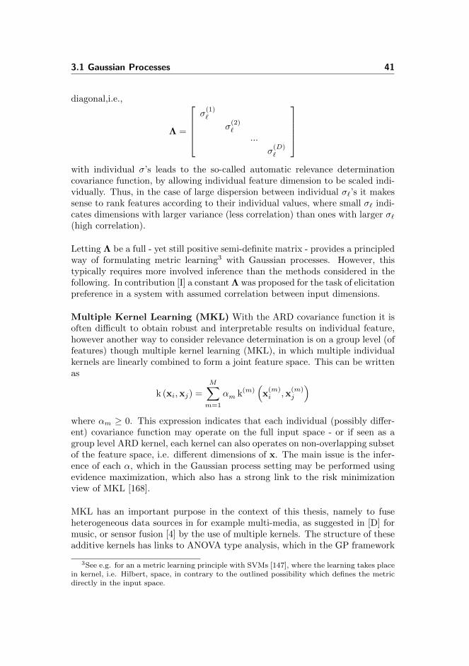
3.1 Gaussian Processes 41
diagonal,i.e.,
Λ =
σ(1)`
σ(2)`
...
σ(D)`
with individual σ’s leads to the so-called automatic relevance determinationcovariance function, by allowing individual feature dimension to be scaled indi-vidually. Thus, in the case of large dispersion between individual σ`’s it makessense to rank features according to their individual values, where small σ` indi-cates dimensions with larger variance (less correlation) than ones with larger σ`(high correlation).
Letting Λ be a full - yet still positive semi-definite matrix - provides a principledway of formulating metric learning3 with Gaussian processes. However, thistypically requires more involved inference than the methods considered in thefollowing. In contribution [I] a constant Λ was proposed for the task of elicitationpreference in a system with assumed correlation between input dimensions.
Multiple Kernel Learning (MKL) With the ARD covariance function it isoften difficult to obtain robust and interpretable results on individual feature,however another way to consider relevance determination is on a group level (offeatures) though multiple kernel learning (MKL), in which multiple individualkernels are linearly combined to form a joint feature space. This can be writtenas
k (xi,xj) =
M∑
m=1
αm k(m)(x
(m)i ,x
(m)j
)
where αm ≥ 0. This expression indicates that each individual (possibly differ-ent) covariance function may operate on the full input space - or if seen as agroup level ARD kernel, each kernel can also operates on non-overlapping subsetof the feature space, i.e. different dimensions of x. The main issue is the infer-ence of each α, which in the Gaussian process setting may be performed usingevidence maximization, which also has a strong link to the risk minimizationview of MKL [168].
MKL has an important purpose in the context of this thesis, namely to fuseheterogeneous data sources in for example multi-media, as suggested in [D] formusic, or sensor fusion [4] by the use of multiple kernels. The structure of theseadditive kernels has links to ANOVA type analysis, which in the GP framework
3See e.g. for an a metric learning principle with SVMs [147], where the learning takes placein kernel, i.e. Hilbert, space, in contrary to the outlined possibility which defines the metricdirectly in the input space.
42 Preference Learning with Gaussian Processes
can be obtained through the use of additive kernels [59] allowing interpretationof complex interactions between individual features.
Multi-Task (MTK) The GP covariance function further provides a simple,but easy and intuitive way of defining a multi-task model, without resorting tomore advanced hierarchical structures such as [22]. The simplest form of suchmulti-task kernel was proposed in [32] and is simply given by a product kernel
k(xi,xj
)= k
([x
(a)i ,x
(b)i ]>, [x
(a)j ,x
(b)j ]>)
(3.6)
= k(x
(a)i ,x
(a)j
)k(x
(b)i ,x
(b)j
)
This means that the kernel matrix can be written as the Kronecker productbetween the two individual kernel matrices, i.e. K = K(a) ⊗ K(b) yieldinga relative easy implementation. A comprehensive review of such multi-taskmethods is given in [5] in the setting of multiple output learning with generalkernel methods.
The multitask-kernel approach provides a simple way of defining a multi-usermodel by correlating user by their features x(user), as applied in contribution[J]. However, more elaborate methods has been prosed for the particular task forpreference learning such as an hierarchical approach [24], and a more traditionalcollaborative filtering approach [93] comparing the aforementioned methods.
Probability Product Kernel (PPK) The PPK kernel [97] (as previouslymentioned in connection with audio modelling) is an elegant method for com-bining the discriminative nature of the Gaussian process model with generativeproperties of the input data by directly defining the covariance functions as theinner product between two probability distributions, p(x|θ) and p(x|θ′), i.e.,
k(p (x|θ) , p
(x|θ′
))=
∫ (p (x|θ) p
(x|θ′
))1/qdx
where q > 0. In effect this implies that each object can be represented by aprobability distribution, which is highly relevant for audio where models suchas Gaussian mixture models, Markov models and even Hidden Markov Models(HMM) are frequently used models of low levels audio features as outlined inSec. 2). In contribution [F]D, the PPK was used based on GMM models forindividual audio objects.
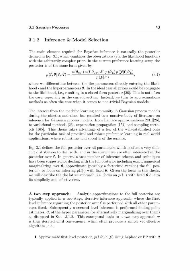
3.1 Gaussian Processes 43
3.1.2 Inference & Model Selection
The main element required for Bayesian inference is naturally the posteriordefined in Eq. 3.1, which combines the observations (via the likelihood function)with the arbitrarily complex prior. In the current preference learning setup theposterior is of the same form given by,
p (f ,θ|Y,X ) =p (θGP) p (f |θGP ,X ) p (θL) p (Y|f ,θL)
p (Y|X ), (3.7)
where we differentiate between the the parameters directly entering the likeli-hood - and the hyperparameters θ. In the ideal case all priors would be conjugateto the likelihood, i.e., resulting in a closed form posterior [26]. This is not oftenthe case, especially in the current setting. Instead, we turn to approximationsmethods as often the case when it comes to non-trivial Bayesian models.
The interest from the machine learning community in Gaussian process modelsduring the nineties and since has resulted in a massive body of literature oninference for Gaussian process models: from Laplace approximations [231][26],to variational methods [26], expectation propagation [154] and sampling meth-ods [165]. This thesis takes advantage of a few of the well-established onesfor the particular task of practical and robust preference learning in real-worldapplications, where robustness and speed is of the essence.
Eq. 3.1 defines the full posterior over all parameters which is often a very diffi-cult distribution to deal with, and in the current we are often interested in theposterior over f . In general a vast number of inference schema and techniqueshave been suggested for dealing with the full posterior including exact/numericalmarginalizing over θ, approximate (possibly a factorized version) the full pos-terior - or focus on inferring p(f |·) with fixed θ. Given the focus in this thesis,we will describe the the latter approach, i.e. focus on p(f |·) with fixed θ due toits simplicity and effectiveness.
A two step approach: Analytic approximations to the full posterior aretypically applied in a two-stage, iterative inference approach, where the firstlevel inference regarding the posterior over f is performed with all other param-eters fixed. Subsequently a second level inference is performed finding pointestimates, θ, of the hyper parameter (or alternatively marginalizing over them)as discussed in Sec. 3.1.2. This conceptual leads to a two step approach wis then iterated until convergence, which often provides a simple yet effectivealgorithm , i.e.,
I Approximate first level posterior, p(f |θ,X ,Y) using Laplace or EP with θ
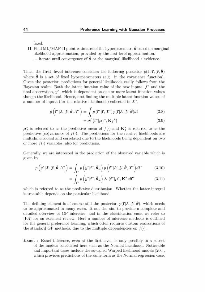
44 Preference Learning with Gaussian Processes
fixed.
II Find ML/MAP-II point-estimates of the hyperparemetrs θ based on marginallikelihood approximation, provided by the first level approximation.
... iterate until convergence of θ or the marginal likelihood / evidence.
Thus, the first level inference considers the following posterior p(f |X ,Y, θ)
where θ is a set of fixed hyperparameters (e.g. in the covariance function).Given the posterior, predictions for general likelihoods easily follows from theBayesian realm. Both the latent function value of the new inputs, f∗ and thefinal observation, y∗, which is dependent on one or more latent function valuesthough the likelihood. Hence, first finding the multiple latent function values ofa number of inputs (for the relative likelihoods) collected in X ∗,
p(f∗|X ,Y, θ,X ∗
)=
∫
f
p (f∗|f ,X ∗) p(f |X ,Y, θ)df (3.8)
= N(f∗|µf ∗,Kf
∗) (3.9)
µ∗f is referred to as the predictive mean of f(·) and K∗f is referred to as thepredictive (co)variance of f(·). The predictions for the relative likelihoods aremultidimensional and correlated due to the likelihoods being dependent on twoor more f(·) variables, also for predictions.
Generally, we are interested in the prediction of the observed variable which isgiven by,
p(y∗|X ,Y, θ,X ∗
)=
∫
f∗p(y∗|f∗, θL
)p(f∗|X ,Y, θ,X ∗
)df∗ (3.10)
=
∫
f∗p(y∗|f∗, θL
)N (f∗|µ∗,K∗)df∗ (3.11)
which is referred to as the predictive distribution. Whether the latter integralis tractable depends on the particular likelihood.
The defining element is of course still the posterior, p(f |X ,Y, θ), which needsto be approximated in many cases. It not the aim to provide a complete anddetailed overview of GP inference, and in the classification case, we refer to[167] for an excellent review. Here a number of inference methods is outlinedfor the general preference learning, which often requires custom realizations ofthe standard GP methods, due to the multiple dependencies on f(·).
Exact : Exact inference, even at the first level, is only possibly in a subsetof the models considered here such as the Normal likelihood. Noticeableand important cases include the so-called Warped likelihood models [200],which provides predictions of the same form as the Normal regression case.

3.1 Gaussian Processes 45
Laplace : The Laplace approximation is a general tool for approximating in-tractable integrals. For GP based models, the starting point is the firstlevel posterior. This posterior is approximated by a second order Tay-lor expansion around the mode, which provides a multivariate Gaussianapproximation, i.e,
q (f | X ,Y,θ) , N(f |f ,A−1
)(3.12)
where f denotes the mode and A denotes the covariance matrix of themultivariate approximation. Thus, the main task is to find the mode andthe covariance matrix for this approximating distribution, which in turnbecomes an optimization problem. This is a standard problem of momentmatching, which is done by considering the unnormalized log-posterior andits first two derivatives. If the log-likelihood is log-concave this is a convexproblem and can be solved by standard Newton step [182, Sec.3.4.1].
The standard Laplace approximation for binary classification with Gaus-sian processes [182, Sec.3.4.1], i.e., the model denoted as absolute-discrete-bounded-probit in Fig.3.3, assumes that the Hessian of the cost function isdiagonal since the likelihood only depends on one variable, f(x). However,in the preference learning scenario with relative models (relative-discrete-pairwise, BTL and Planket-Luce) this does not hold true, and custom im-plementation is required. The Laplace approximation was suggested forthe pairwise probit model in [48], and the setup presented in Tab.3 con-tains a general Laplace implementation supporting both absolute, relativeobservation for both the pairwise, and the general BTL and Plackett-Lucemodels. For robustness and fast convergence, the setup has the optionto use a damped Newton step. Furthermore, for non-log concave likeli-hoods the setup applies a simple but effective methods of thresholds thesecond derivative of the likelihood function as suggested in [232] to obtaina robust approximation, despite possibly non-unique solutions.
The Laplace approximation is also directly applied in approximate themarginal likelihood - or evidence - defined by the integral in Eq. 3.2.
Expectation Propagation : The Laplace approximation is a simple, but ef-fective approximation method and relatively fast to derive for a number ofnew models based on the setup in Tab. 3.1, however, it simply assumes alocal expansion around the mode of the posterior. The EP does not makethis local assumption and considers a factorized posterior with individualapproximations to each likelihood terms. The approximation can thus bewritten as
q (f |X ,Y) ,1
ZEPp (f)
∏tk
(fk|µk, Σk, Zk
)= N (µEP ,ΣEP ) , (3.13)

46 Preference Learning with Gaussian Processes
where tk
(fk|µk, Σk, Zk
)is the approximation to each likelihood term and
taken to be a (unnormalized) Gaussian distribution. ZEP is a global nor-malizing term ensuring that the global multivariate Gaussian approxima-tion is consistent, i.e., integrates to one. In the case of relative observationswith more than one f(·) variable in each likelihood term, the tk terms be-comes an (unnormalized) multivariate Gaussian distribution.
The inference then amounts to estimating the so-called site parameters,µk and Σk which is done using the fixed-points algorithm proposed in[154] consisting of the following steps
For each observation k ∈ [1 : K]
1 q/k (f)← q (f |·) /tk (f |·) =∏k 6=l
tl (fl|·)
2 tknew (fk|·)← arg min
tk(fk|·)DKL
(p (yk|f) q/k (f) ||tk (fk|·) q/k (f)
)
3 q (f)← tknew (fk|·) q/k (f)
...repeat until convergence
where q/k is used to denote that the likelihood term originating from obser-vation k has been removed. The minimization of the KL divergence (DKL)in step 2 is a matter of moment matching since using the (un)normalizedGaussian distribution as site approximation.
The setup in Tab.3 includes a custom EP implementation for the discretepairwise probit model, which is an extended version of the standard EPmodels for probit models originally proposed in [46], alltough EP inferencefor general relative models is not currently supported.
It should be emphasized that EP can be used in a ’online’ setting [53] inwhich the iteration only runs for a single sweep though all the data points[53]. This, however, still requires maintaining the site parameters for allthe observations.
Sampling A different approach, not considered in detail in the thesis, is toperform inference through simulation by drawing Ns samples, f (s), fromthe posterior in Eq. 3.1, from which we can evaluate the moments of theposterior of both the latent variables, f , and the hyperparameters, θ andcan in turn calculates expectations of for example the first level posterior
as, Ep(f |X ,Y,θ){f} ≈ 1Ns
Ns∑s=1
f (s).
Sampling in Gaussian process models is usually performed using variationsof Markov Chain Monte Carlo (MCMC) methods as outlined in [165] pos-sibly combined with other sampling steps such as slice sampling [162] forsampling hyperparameters. Given the applied nature of the preferencelearning setup, sampling is only used for evaluation of other approxima-tion, i.e., as a golden standard.

3.1 Gaussian Processes 47
The particular inference approach used for estimating p(f |·) is typically depen-dent on the actual likelihood / model, but the applications considered in thecontributions usually rely on the relatively simple Laplace approximation, whichhas proven a easy, reliable and robust method for the relative models.
Hyperparameters and Model Selection In the two step procedure out-lined above, the first level inference focused (mainly) on the posterior of f , i.e.
p(f |X ,Y, θ), however, the hyperparameters, θ, are as mentioned also criticalmodel parameters (as indicted by the full posterior in Eq. 3.1) and should inprinciple not be considered any different than f in a full Bayesian treatment.If we do not need to infer actual values/distributes for the hyperparameters,we may marginalize over them either as part of part of a full MCMC infer-ence step or a combination with the level one analytical/approximation, and/ornumerical methods.
However, in the two-step approach which is the focus, we may turn to a op-timization approach which is an effective alternatively to the often computa-tional expensive marginalization approach. We thus abandon the full Bayesianschema indicated by Eq. 3.7 and aim only a a single ’good’ point estimate forthe hyperparameters. This corresponds to the second level of inference out-lined above, and is based on the notion of model evidence and Bayesian modelcomparison.
The model evidence - or marginal likelihood - is an important and and muchdebated entity in the Bayesian framework. The marginal likelihood is a expres-sion of how likely it is to generate the given data, D, given a particular modeland model parameters [26]. So if the hyperparameters are fixed, we may con-duct Bayesian model comparison by the ratio between the marginal likelihoodresulting in the so-called Bayes factor,
BF =p (Y|X ,M1)
p (Y|X ,M2)=
∫p (Y|f) p (f |X ,M1) df∫p (Y|f) p (f |X ,M2) df
If the true data generating distribution is contained in the model this factor canon average be shown to select the correct model [26]. Hence, the model withthe highest marginal likelihood is preferred and finding the ’best’ point value ofthe hyper parameters,θ, can be an integrated part of the inference by directlyoptimizing the marginal likelihood as part of the inference. This procedure isknown under different names including maximum likelihood II (ML-II), empir-ical Bayes [41] or in the machine learning literature as evidence optimization[136].
The second level inference/estimation therefore involves finding point esti-
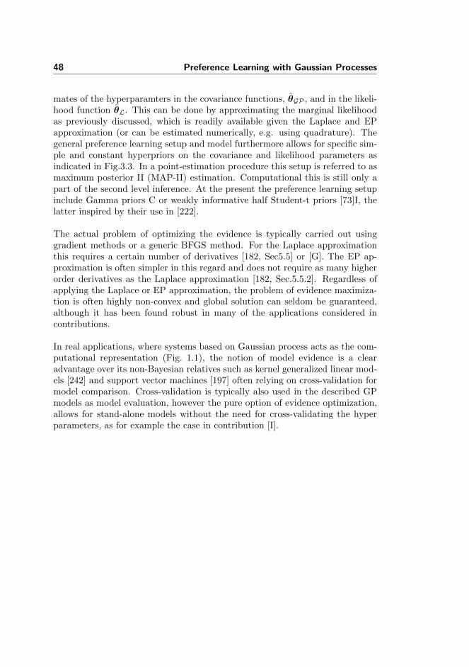
48 Preference Learning with Gaussian Processes
mates of the hyperparamters in the covariance functions, θGP , and in the likeli-hood function θL. This can be done by approximating the marginal likelihoodas previously discussed, which is readily available given the Laplace and EPapproximation (or can be estimated numerically, e.g. using quadrature). Thegeneral preference learning setup and model furthermore allows for specific sim-ple and constant hyperpriors on the covariance and likelihood parameters asindicated in Fig.3.3. In a point-estimation procedure this setup is referred to asmaximum posterior II (MAP-II) estimation. Computational this is still only apart of the second level inference. At the present the preference learning setupinclude Gamma priors C or weakly informative half Student-t priors [73]I, thelatter inspired by their use in [222].
The actual problem of optimizing the evidence is typically carried out usinggradient methods or a generic BFGS method. For the Laplace approximationthis requires a certain number of derivatives [182, Sec5.5] or [G]. The EP ap-proximation is often simpler in this regard and does not require as many higherorder derivatives as the Laplace approximation [182, Sec.5.5.2]. Regardless ofapplying the Laplace or EP approximation, the problem of evidence maximiza-tion is often highly non-convex and global solution can seldom be guaranteed,although it has been found robust in many of the applications considered incontributions.
In real applications, where systems based on Gaussian process acts as the com-putational representation (Fig. 1.1), the notion of model evidence is a clearadvantage over its non-Bayesian relatives such as kernel generalized linear mod-els [242] and support vector machines [197] often relying on cross-validation formodel comparison. Cross-validation is typically also used in the described GPmodels as model evaluation, however the pure option of evidence optimization,allows for stand-alone models without the need for cross-validating the hyperparameters, as for example the case in contribution [I].
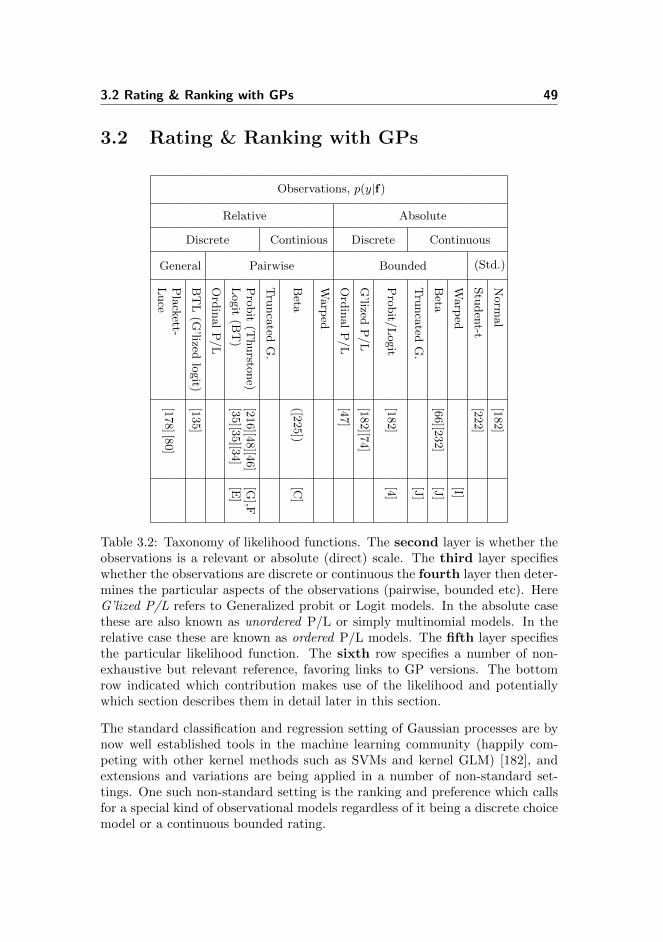
3.2 Rating & Ranking with GPs 49
3.2 Rating & Ranking with GPs
Observations, p(y|f)
Absolute
Continuous
(Std.)
Norm
al
[182]
Student-t
[222]
Bounded
Warp
ed[I]
Beta
[66][2
32]
[J]
Truncated
G.
[J]
Discrete
Probit/
Logit
[182]
[4]
G’lized
P/L
[182][7
4]
OrdinalP/L
[47]
Relative
Continious
Pairwise
Warp
ed
Beta
([225])
[C]
Truncated
G.
Discrete
Probit
(Thursto
ne)
[216][4
8][4
6]
[G],F
Logit
(BT)
[35][3
5][3
4]
[E]
OrdinalP/L
General
BTL(G
’lizedlogit)
[135]
Plackett-
[178][8
0]
Luce
Table 3.2: Taxonomy of likelihood functions. The second layer is whether theobservations is a relevant or absolute (direct) scale. The third layer specifieswhether the observations are discrete or continuous the fourth layer then deter-mines the particular aspects of the observations (pairwise, bounded etc). HereG’lized P/L refers to Generalized probit or Logit models. In the absolute casethese are also known as unordered P/L or simply multinomial models. In therelative case these are known as ordered P/L models. The fifth layer specifiesthe particular likelihood function. The sixth row specifies a number of non-exhaustive but relevant reference, favoring links to GP versions. The bottomrow indicated which contribution makes use of the likelihood and potentiallywhich section describes them in detail later in this section.
The standard classification and regression setting of Gaussian processes are bynow well established tools in the machine learning community (happily com-peting with other kernel methods such as SVMs and kernel GLM) [182], andextensions and variations are being applied in a number of non-standard set-tings. One such non-standard setting is the ranking and preference which callsfor a special kind of observational models regardless of it being a discrete choicemodel or a continuous bounded rating.

50 Preference Learning with Gaussian Processes
The related contributions applies and proposes a number observational modelsfor Gaussian processes in the model defined in Fig. 3.1. In the following the themost often applied models are outlined and motivated.
3.2.1 Relative-Discrete-Pairwise-Probit/Logit Model
One of the most popular experimental paradigms for eliciting perceptual andcognitive effects is the two alternative forced choice, i.e., the choice set consist oftwo objects xuk
∈ X and xvk ∈ X . These are presented to a subject and askinghim/her to select one, i.e., yk ∈ {−1, 1}. By repeating this for many differentobjects results in K responses on pairwise comparisons between any two inputsin X , Y = {(yk;xuk
, xvk)|k = 1, ...,K}
A classic modelling approach towards such pairwise choices is based on Thur-stone’s ”law of comparative judgements” in which the choice is assumed to bethe effect of internal but noisy utilities for each object, i.e., the utility for anobject xu is f(xu) + εu and the utility for object xv is f(xv) + εv where ε isthe noise. The general starting point for both the probit and pairwise choicemodels comes from considering the probability of a subject selecting xu, i.e.
P (f (xu) + εu > f (xv) + εv) = P (f (xu)− f (xv) > εv − εu) (3.14)
=
∫I (f (xu)− f (xv) > εv − εu) p (ε) dε (3.15)
where I(·) is an indicator function, returning 1 if the argument is true; other-wise zero. The main aspects to consider is the noise distribution, p (ε), on theinternal utilities which effectively leads to difference choice models such as theprobit or logit. In [216] Thurstone suggested a Normal distribution which re-sults in the probit model [30], while the a pairwise logit model assumes ε to belogistically distributed [30][220]. Following Thurstones approach, p(ε), is nor-mally distributed and depending on the assumptions regarding the correlatedvariables; we obtain a number of the case which Thurstone outlines in [216].However, the simplest one, case 5, is derived by assuming that the noise onindividual objects are uncorrelated and have equal variance, σL. Fortunately,this results in the multidimensional integral in Eq. 3.14 being tractable and canbe shown to result in the cumulative Gaussian (the probit model) such that thelikelihood becomes
p (yk|fk, σ) = Φ
(ykf (xuk
)− f (xvk)√2σL
)
with fk = [f (xuk) , f (xvk)]
>. This defines the likelihood (actually the probabil-
ity) of the choice, yk, however the estimation of the function values themselves is

3.2 Rating & Ranking with GPs 51
the main interest here. By assuming uncertainty on the values of f(·), we placethe Gaussian process over the latent function values. Such as model was firstconsidered in [48]. Since the model now has dependencies on two latent functionvalues the graphical chain model is slightly different than in the standard caseand depicted in Fig. 3.3.
The primary model applied in contributions [C],[G][D][F] is the probit choicemodel described above. Compared to the standard setup proposed in [48], weallow for simple priors on the hyperparameters, which has been found useful androbust in many of the applications. Assuming a squared exponential covariancefunction [182, Cha.4], with two hyper parameters, σ` and σs, the combinedmodel can be specified as
σs|ξs ∼ half Student-t /Gamma
σ`|ξ` ∼ half Student-t /Gamma
fk|σs, σ` ∼ GP(
m (xk) , k (xk, ·)σs,σ`
)
πk|fk, σL = Φ (f (xuk)− f (xvk))
yk ∼ Bernoulli (πk)
where ξ is a set of parameters in the hyperprior, for example scale and degreeof freedom parameters for the half Student-t prior [73].
This model requires approximation of the posterior, and the setup currentlysupports both Laplace and EP. Predictions for a new choice set C = {xr,xs}is (with the Gaussian approximation) analytical in the form of a cumulativeGaussian.
Figure 3.3: Graphical chain representation of the pairwise model. Compared tothe standard GP classification model, the output variables y now each dependon multiple f variables.

52 Preference Learning with Gaussian Processes
3.2.2 Relative-Continuous-Pairwise-Beta Model
The classic probit likelihood is mainly chosen for its robustness compared to e.gcontinuous/absolute scaling experiments. However, the pairwise comparisons ispotentially a slow way of learning in a high-dimensional input space and withmany objects to consider. It may therefore be advantageous to exploit the extrainformation from continuous responses to get a faster method for preferenceelicitation without jeopardizing the robustness from standard binary responses.This can be done by observing a degree to which either is preferred alongsidethe binary decision of xu and xv. Such a setting is some times refereed to assureness or confidence [230]. In the preference learning scenarios, we refer to itas degree of preference (DoP).
To address this setting a continuous, but bounded response y ∈ ]0; 1[ is defined,observed when comparing the two options in xu and xv. The first option, xu, ispreferred for y < 0.5. The second option, xv, is preferred for y > 0.5 and noneis preferred for y = 0.5. Hence, the response captures both the choice betweenxu and xv, and the degree of the preference. One could consider the two choicesseparately and assume that continuous DoP choice always follows the binarychoice such that it can not change the binary choice to ensure robustness. Thiscan however easily be shown to lead to the same modelling considerations.
Modelling this type of continuous response is slightly more involved than mod-elling the discrete choice in the discrete pairwise case. First of all, the likelihoodmust adhere to the binary choice and furthermore be bounded in its supportsince y ∈]0, 1[. In contribution [C], we proposed a model using a Beta typedistribution with its mean parameterized by the cumulative Gaussian functionthrough the shape parameters α and β. The general model can be written
σs|ξs ∼ half Student-t /Gamma
σ`|ξ` ∼ half Student-t /Gamma
fk|σs, σ` ∼ GP(
m (xk) , k (xk, ·)σs,σ`
)
β(fk) = ν(1− µ(fk)), α(fk) = νµ(fk)
yk ∼ Beta (α(fk), β(fk)) (3.16)
Where ν relates to the precision of the Beta distribution and is not parame-terized by f . The shape parameters of the Beta distribution is a function ofof the GP, and we applied a well-known re-parametrization of the Beta distri-bution [66]. The mean function of the Beta distribution is given as µ (fk, σ) =
Φ(f(vk)−f(uk)√
2σ
). The precision term ν in Eq. 3.16 is inversely related to the
observation noise on the continuous bounded responses. In general, ν, can be

3.2 Rating & Ranking with GPs 53
viewed as a measure of how consistent the scale is used in a given comparison.4.
Approximation for this model is primarily based on the Laplace approximation.Despite the Gaussian approximation predictions are problematic due to theBeta distribution. The probability for yk > 1/2 defines the binary choice ofoption xu and must be evaluated by numerical methods, whereas the binarychoice itself i.e. the hard choice of either xu or xv can easily be evaluated dueto the symmetric likelihood. However, the expectation of y can be evaluatedanalytical due to the specific parametrization which provides insight into theeffective choice model, a topic for further investigation (see [J]). Alternatively,
one may rely on maximum-a-posterior analysis of p(f |X ,Y, θ) which provides aclosed form expression [C], but compromises the Bayesian principle.
In the applied versions of the model ([C] and [170]) the warping function, whichmaps the latent function to the likelihood, has been limited to a single fixedcumulative Gaussian based on the principle from standard choice models. How-ever, a more general warping (or cumulative link) function is the (so far finite)
sum of such functions, i.e., g (f(x)) =∑Ng
i=1 Φ (f(x)|µi, σi), which includes find-ing the parameters of the warping function by evidence optimization. Veryrecent advances in warped GPs has furthermore shown potential to use non-parametric functions for the warping potentially generalizing many of the out-lined models relying on some kind of link or warping function [122].
3.2.3 Absolute-Continuous-Bounded Beta Model
Modeling absolute bounded responses, e.g. y ∈]0; 1[, has relevance to manyapplications in finance, survival analysis, and here preference learning, whereusers are asked to rate object on an absolute scale which is inherently bounded.In [J], a Gaussian process model was proposed for modelling continuous ratingson bounded scales for a particular dataset based on Beta and Truncated Gaus-sian distributions. Thus, the setting strongly resembles the classical regressioncase with Gaussian likelihood [182] or Student-t likelihoods [223] - but with abounded support.
4In memorandum, it is noted that a similar likelihood has been proposed for generalizedlinear models but not realized or evaluated in [225]
54 Preference Learning with Gaussian Processes
The model can be written
σs|θs ∼ half Student-t / Gamma (3.17)
σ`|θ` ∼ half Student-t / Gamma (3.18)
fk|σs, σ` ∼ GP(
m (xk) , k (xk, ·)σs,σ`
)(3.19)
β(fk) = ν(1− µ(fk)), α(fk) = νµ(fk)
yk∼ Beta (α(fk), β(fk)) (3.20)
The idea is similar to the pairwise Beta model used for relative modelling de-scribed in 3.2.2, i.e., parameterizing the mean of the Beta distribution withthe latent Gaussian process though a warping function given by the cumulativeGaussian.
The inference is based on the Laplace approximation or the EP approximationin which a numerical integration is used to evaluate the partition function (see[J]) for details. The model is in essence a non-parametric version of the modelproposed in [66] also extended to support Truncated Gaussian observations byparameterizing the mean or the mode of the Truncated Gaussian distribution[J].
The models has a strong link to Copular processes (e.g. [232]) which will notbe explored further in the present thesis, but is topic for further investigation.
3.2.4 Releative-Discrete-General Bradley-Terry-Luce andPlackett-Luce
The pairwise model applying probit and logit models is limited by the amountof information each experiment yields. It is possible to extend both the probitand the logit (Bradley Terry) model to multiple alternatives, i.e. C-alternativeforced choice forced [220]. However, the generalized probit results in a likelihoodwhich needs to be evaluated analytically, we therefore focus on the extension ofthe logit model as proposed by Luce [135], which results in analytical likelihoods.The Bradley-Terry-Luce (or ordered generalized logit) is defined as
p (yk ∈ [1 : C] |fk) =ef(xy
k
)∑Ci e
f(xi)
Inference in the Bradley-Terry-Luce (BTL) model is challenging, due to themany dependencies in the likelihood, however, in the Laplace case this doesnot matter due to the global approximation of the posterior, i.e. there is no
3.2 Rating & Ranking with GPs 55
approximation to each term, and the first level approximation simply requiresthe first and second derivative with regards to all variables entering into theeach likelihood term.
The Plackett-Luce (or exploded logit) now effectively extends the BTL in defin-ing a model over permutations given as [178],
p (yk|fk) =C−1∏
j=1
ef(xy
k(j)
)∑Ci=j e
f(xy
k(i)
)
where yk is a permutation of the C object in the choice set, e.g. yk = {4, 2, 3, 1}.Analytical probabilistic predictions are currently made on the pairwise level, i.e.resulting in the standard pairwise logit and applying the logit approximation in[182] also used in the GPML toolbox [67]. Probabilistic predictions for a fullpermutation is based on simulation. Alternative MAP predictions may prove ause full, however, enumerating all possible permutations is still a cumbersometask, which requires further investigation.
The Laplace approximation provides a stating point for examining the PlackettLuce model for preference learning in real-applications, however other approxi-mations should certainly be explored. Some work on the Plackett-Luce modelshas shown a potential route for such work in terms of a EP version for a non-GPversion of the model [80].
3.2.5 Additional Models
The specific models outlined above provides a non-exhaustive, but general overviewto modelling within the setup defined in Fig. 3.1.
Not yet realised observational models, include the ordinal likelihoods (also knownas cumulative link models) previously considered in the GP literature [47] forabsolute settings. This is highly relevant to ratings both in the pairwise andabsolute case since many experimental paradigms consider e.g. the Likert scale[128], where the scale is divided into discrete intervals.
The observation/response types outlined in Tab. 3.2 covers the ones encoun-tered and found relevant during the construction of the setup, however manymore variations may be considered for modelling real-world scenarios, includingtriangle tests, odd-one-out and other experimental paradigms [16] where theGaussian process approach may very well provide a flexible modelling frame-work.

56 Preference Learning with Gaussian Processes
3.3 Sequential Design & Sparsity
The motivation for the setup presented in Fig.3.3 is based on elicitation of vari-ous aspects of human perceptual and cognition through experimental. However,just one experiment, involving human users, can be both costly and time con-sumption. In real applications, it is therefore important to minimize the burdenfor the users and the computational time required. This can be done by mini-mizing the number of experiments which potentially limits the information. Analternative method is socalled sequential design - or active learning - in whichexperiments are proposed as the ratings come in and the models gets better.This will optimally ensure that the system does not require more experimentsthan needed in order to solve the task and find a appropriate model. However,while GP based classification and regression models often perform better orsimilar to other models regardless of the setting [182], a price is often paired interms of the computational requirements due to an inherently O(N3) scaling interms of the number of labeled examples. These two aspects can both been seenas a way to reduce the number of inputs, but from two different perspectivesoutlined as follows;
Directly: The experimental design used to obtain the data obviously deter-mines how many observations are obtained. Directly limiting the numberof observations can roughly be performed in two ways:
a From a fixed set of labeled points include only a subset, the activeset.
b From a (infinite) set of unlabeled inputs obtain only labels/values fora subset (and include in the dataset).
An overview and review is provided in 3.3.1 placing methods applied con-tribution [I] in context with other methods in the field.
Indirectly: Modelling can reduce the effective number of points which is heregenerally refereed to as sparsity which also was two approaches: 5.
b Inducing: Define the number of effective points (and locate themanywhere according to some measure of performance). An overviewand review provided in 3.3.2 placing contribution [H] in context.
a Inferred: Infer the number of points, often a subset of the originalinputs. Examples are Support Vector Machines and the ReleveanceVector Machines (RVM) [217]. This setting is not considered in thecurrent thesis.
5The orthogonal notion of sparsity, obtained by removing individual feature dimensions isnot considered here (see e.g. the ARD kernel)
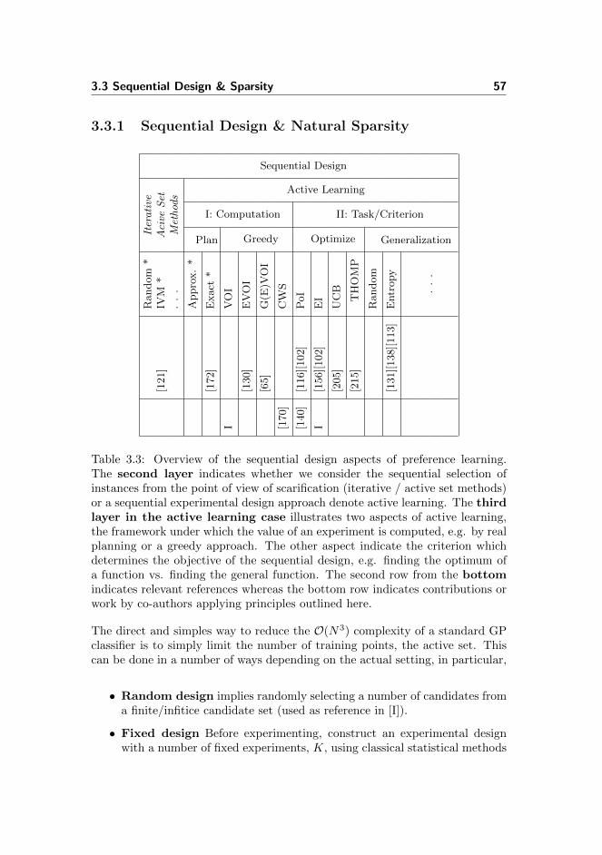
3.3 Sequential Design & Sparsity 57
3.3.1 Sequential Design & Natural Sparsity
Random
*Iterative
Sequential Design[121]
IVM
*Acive
Set
...
Methods
Approx.*
Plan
I: Computation
Active Learning
[172]
Exact
*
IVOI
Greedy[130]
EVOI
[65]
G(E
)VOI
[170]
CW
S
[140]
[116][102]
PoI
Optimize
II: Task/Criterion
I[156][102]
EI
[205]
UCB
[215]
THOMP
Random
Generalization
[131][138][113]
Entropy
...
Table 3.3: Overview of the sequential design aspects of preference learning.The second layer indicates whether we consider the sequential selection ofinstances from the point of view of scarification (iterative / active set methods)or a sequential experimental design approach denote active learning. The thirdlayer in the active learning case illustrates two aspects of active learning,the framework under which the value of an experiment is computed, e.g. by realplanning or a greedy approach. The other aspect indicate the criterion whichdetermines the objective of the sequential design, e.g. finding the optimum ofa function vs. finding the general function. The second row from the bottomindicates relevant references whereas the bottom row indicates contributions orwork by co-authors applying principles outlined here.
The direct and simples way to reduce the O(N3) complexity of a standard GPclassifier is to simply limit the number of training points, the active set. Thiscan be done in a number of ways depending on the actual setting, in particular,
• Random design implies randomly selecting a number of candidates froma finite/infitice candidate set (used as reference in [I]).
• Fixed design Before experimenting, construct an experimental designwith a number of fixed experiments, K, using classical statistical methods

58 Preference Learning with Gaussian Processes
of experimental design [158]. This could be performed using factorialdesigns or combinational design like Latin squares [158]. For standardGP regression with fixed hyper parameters, this may even be specifiedbeforehand by selecting the design that minimizes the posterior/predictiveentropy/variance 6.
• Iterative/Active Set methods is the general setting where the algo-rithm (iteratively) either removes or adds labeled points based on somecriterion from a fixed candidate set, such as the Informative Vector Ma-chine (IVM) and its predecessors [121],[191][192] and the recently proposedapproach considering the predictive uncertainty [86]. In general, this prin-ciple is characterized by the label being known for all candidate points.
• Active Learning/Sequential Design or interactive learning impliesthat experiments are added sequentially based on some criterion, which isdependent, in some way, on the current model posterior and/or predictivedistribution. This setting is typically characterized by the fact that thelabel of the experiments are unknown before experimentation. This is thecase for all intended purposes of the preference learning setup.
The differentiating property between iterative set vs. active learning is thus,whether the label is known for the candidate set or not. While iterative/activeset methods are certainly interesting; the main interest is the active learningsetting since human labels are often difficult to obtain. Furthermore, the ap-plication is typically intended for novel situation where where no labels areavailable at all. In this situation a clear advantage of GPs over non-Bayesianmodels is the representation of both posterior and predictive uncertainly, whichmakes them highly suitable for introducing active learning/sequential designwith the purpose to learn as efficient/fast as possible based on some notion ofgain in information.
Sequential Design / Active Learning
This section continues with a general overview of active learning or sequen-tial design in the GP setting. This includes a general view of many of thestand-alone contribution in the applied GP literature. First, we differentiatebetween two aspects outlined in Tab. 3.3, namely computation and criterion,which together defines how the value of conducting an experiment is evalu-ated. An experiment is in the GP setting a number of inputs which is part
6Since the predictive variance does not depend on the actual response, y, as seen fromEq.3.3

3.3 Sequential Design & Sparsity 59
of the experiment, i.e. one, two or more candidate input points collected inE = {x∗1,x∗2, ...,x∗E}.
The main setting considered here is the greedy one-step-ahead selection of ex-periments7, thus the aim is to considering the next experiment only - not con-sidering multiple steps ahead which refereed to as planning in Tab. 3.3
Many of the current methods in the GP literature [96][113][31] can be seen asreductions of the following general formulation
∂
∂E
∫p(yk|Ek,D)︸ ︷︷ ︸prior predictive
× U(p (f |D)︸ ︷︷ ︸prior
p (fEk|Ek, D) , p (yk|Ek, D)︸ ︷︷ ︸prior predictive
p (f |yk, Ek,D)︸ ︷︷ ︸posterior︸ ︷︷ ︸
V OI
)dy
︸ ︷︷ ︸EV IO︸ ︷︷ ︸
G(E)V IO
(3.21)
The G(E)VIO refers to the gradient of the VIO / EVIO function (as mentionedin [172]). The EVOI formulation is nothing more than a formulation of Lindley’sexpected information of an experiment (see e.g. [131][130, Sec. 12])8. Theaddition of the gradient version G(E)VOI is mainly computational, whereas thepossible reduction to VOI can be both an explicit utility choice or computationalissue.
Experiments are selected in a greedy fashion by either of the four options out-lined
arg maxE
VIO (E) argE
GVIO (E) = 0
∣∣∣∣E0
(3.22)
arg maxE
EVIO (E) argE
GEVIO (E) = 0
∣∣∣∣E0
(3.23)
where E0 indicates the starting position of a gradient search. The function anddistribution involved are:
• U(·) defines the actual criterion/utility based on all or a subset of thelisted arguments in Eq. 3.22.
7This is strictly not a requirement since many of the methods considered can be generalizedto a dynamic programming setting however of course at an increased cost. See e.g. [71][172]for examples for such an approach
8In the view of inference, not the decision theoretic view in which a decision loss is alsodefined [130, Sec. 4]

60 Preference Learning with Gaussian Processes
• p (f |D) is the current prior over the function (after seeing the data D, butbefore seen a new candidate experiment).
• p (fk|Ek,D) given the current prior, this is the predictive distribution for
the function values for the inputs in the candidate experiment. This iscalled the prior predictive distribution.
• p (yk|Ek,D) based on the p (fk|Ek,D) and the likelihood function this is
the predictive distribution for the observed variable y.
• p (f |yk, Ek,D) after seeing the response yk for the experiment Ek, we canform the posterior, potentially needs to be approximated.
The criterion defining the utility function, U(·), is obviously a critical algo-rithm/model choice and often dependent on the particular use of the resultingmodel. If the aim is to learn a ’good’ model for the entire (feasible) input spacethen, one should chose a criterion which ensures good generalization, often for-mulated in terms of the parameters, i.e. f()9. If the task, on the other hand,is to find input instance with the highest latent function value (or observed re-sponse), we should select a criterion which ensures that we find the maximum;not ensure that we learn the overall function. In the preference learning appli-cations there is a need for both and in particular the combination of both (seefor examples of specialized [44] utilities in the Bayesian linear model setting).
In terms of generalization the machine learning litterateurs has considered alarge number of proposals for different models ranging from disagreement byquery-by-committee [195], to minimum margin methods [218], and criterionsbased on statistical notions of uncertainty models such as [49][137]. The latteris a good starting point for the Gaussian process view point, which is based onthe general notion of entropy [50],
(E)VIO Entropy : is a natural measure of information of an experiment whichwas proposed by Lindley in early work [129], where the change in entropybetween prior and posterior over the parameters (here f) was considered.Thus, the criterion U(·) is evaluated as
U (p (f |yk, Ek,D) , p (f |D)) ≡ S (f |yk, Ek,D)− S (f |D) (3.24)
=
∫p (f |yk, Ek,D) log p (f |yk, Ek,D) df
−∫p (f |D) log p (f |D) df (3.25)
9The thesis will not consider utilities regarding the hyperparameters, θ, but [113] considersthis aspects in a Normal regression case. Furthermore, we do not take into account the inputdensity of x, p(x)

3.3 Sequential Design & Sparsity 61
While seeming simple, the first factor in the first integral implies evaluatingthe posterior for each possible outcome y, but by taking the expectationEVIO this can be avoided as seen by Lindley [131], using informationtheoretic arguments, and the EVIO becomes,
EV IO (Ek) ≡∫ ∫
p (fk|Ek,D) p (yk|fk,D) log p (yk|fk,D) dydf (3.26)
−∫p (yk|Ek,D) log p (yk|Ek,D) dy
Thus, no posterior calculation is to be calculated for every possible out-come, however, the first integral still does not (often) result in closedform expressions. Numerical or analytical approximations is often required(currently the first option is a part of the setup). A specific approximationwas proposed recently for probit based models [93]. For the pairwise case(not GPs) this utility was first considered in [75] .
An equivalent information theoretic view10 was taken to yield the same re-sult for the Normal regression case [113] showing general properties of thisin standard regression. They also considering the implications imposed bythe hyperparameters in sequential design.
VOI is often considered in the entropy case by only taking into a accountthe entropy of the predictive distribution over f , and the utility becomes
U (p (fk|Ek,D)) ≡ S (f
k|Ek,D) (3.27)
which does not depend on the observation, yk, and reduces to the VOIsetting. For multiple inputs this requires evaluating the entropy of a multi-variate Gaussian, which is available in closed form [50]. In the case of asingle value likelihood this corresponds to the predictive variance of f∗.
A particular case is obtained for standard regression with a Normal like-lihood, i.e., a single f∗,. Here the entropy is simply a monotone functionof the predictive variance which does not depend on the observation, andthe design can be made before observing any observations. This is alsoknown as variance reduction or uncertainty sampling.
Response entropy: The approach considered so far was framed in termsof the parameter space, i.e., f(·). A different approach is based on the pre-dictive aspect, thus considering the change in entropy between the predic-tive distribution of a particular response y∗ before and after conductingthe experiment. However, the simplest version of this is the VOI set-ting in which the predictive entropy/variance can be used as the utility,U ≡ S (yz|Ek,D) (see e.g. [233] for a short discussion).
10The easiest way to arrive at Eq.3.26 is by using information theoretic arguments withconditional entropies and mutual information.
62 Preference Learning with Gaussian Processes
In the case of optimization; the field of design and analysis of computer exper-iments (DACE) and global optimization has in many years made use of Gaus-sian process models to perform global optimization [96][156][101]. The machinelearning community has adopted many of these methods of which we will reviewa few, most relevant to the preference learning setup.
(E)VIO Probability of Improvement (PoI) is an old [116] yet intuitivemeasure [101], when attempting to optimize the latent function f . Forthe regression case, i.e. a single candidate point in the experiment, it issimply defined as P (f (x∗) ≥ fmax) with x∗ ∈ E and fmax is the currentmaximum of the latent function. For regression this this amounts to eval-uating a simple integral, resulting in a probit function. Seemingly thisapproach has not been investigated together with the relative observationmethods, such as pairwise comparisons.
(E)VIO Expected Improvement (EI) is a criterion for selection new can-didate points taking in to account the potential change for each candidatepoints [156][101][172]. Given the focus on the latent function is typicallyapplied in the VIO setting (and often in normal regression), i.e., basedon the predictive distribution for f(·). First consider the improvement,I, between the candidate point, x∗ and the point with the current max-imum latent value, fmax = f(xmax), thus the improvement is defined,I(x∗) = f(x∗)−f(xmax). Only considering the positive improvement andevaluation the expectation yields,
EI =
∫ ∞
0
I × p(I)dI (3.28)
which is defined as the expected improvement [102][96][156]. Since f(·)and f(x∗) are jointly Gaussian, this results in a closed form expression forthe utility, namely [96]
U ≡ σEI · N(µEIσEI
)+ µEI · Φ
(µEIσEI
)
where µEI = µ∗−µmax and σ2EI = (σ2)∗+σ2
max−2σ,max∗ where µ∗ is the
predictive mean for the candidate points and the σ’ are the variances andcovariances between the currently best input and the candidate.
It is noted that the VIO depends both on the mean and the variance andgets bigger with both, i.e., an trade off between selection candidates withhigh mean value and candidates with high variance. This is often referredto as exploration and exploiting trade-off.
Contribution [D] applies this approach in an interactive system for a pref-erence model with bounded absolute responses. Other applications in ma-chine learning includes [79] for standard regression. [31] applies a variant

3.3 Sequential Design & Sparsity 63
of the expected improvement in a EVIO setting for a pairwise likelihoodwhich is seemingly computation infeasible for large problems.
For completeness, we notice that one could formulate the expected im-provement on a continuous response variable, i.e., maximizing y insteadof f . In GPs where the latent function often close follows the responsevariables through the mean or mode, it is questionable if this is necessaryand even feasible for most specialized likelihoods. Similar ideas has beenproposed in for example [44, Sec 2.4] for standard Bayesian linear models.
UCB-GP : The UCB (Upper Confidence Bound) algorithm is a popular GPalgorithm [205][79] for optimization tasks which effectively combines thepredictive variance and means in order to find the maximum of the latentfunction. While often applied in a heuristic manner, recent and requiredtheoretical work has shown regret bounds for the UCB-GP algorithm [205].
Thompson GP : Thompson Sampling is an old method not specific to Gaus-sian processes and can be applied in more versatile settings than opti-mization with GPs [215][214]. However, in the optimization setting forGP regression; the Thompson approach amounts to sampling a functionfor the full experiment set, E . Hence,
f∗ ∼ p (f∗|E ,X ,Y, θ)f∗ =
[f (x∗1) , f (x∗2) , ..., f (x∗E)
]
x∗ = arg maxx∗
f∗
This has been considered in a few studies for standard regression [132], butnot for the particular use with relative likelihoods, where the proceduremust be altered.
The Thompson sampling approach introduces an implicit exploration el-ements, which is similar to Criterion Weighted Sampling (CWS),which is a heuristic proposal for providing an (extra) exploration elementto any of the criterions above. The principle simply draws a index of thecandidate point xi ∈ E as follows,
i ∼Multinomial(λ)
where
λ (xi∗) =
(E)V OI (xi∗)
∑i′
(E)V OI (xi′∗)
The principle is like many of the other sequential methods, without anytheoretical foundation, and still awaits a full empirical validation. It hasso far been applied by co-authors in [170].
64 Preference Learning with Gaussian Processes
3.3.2 Induced Sparsity
Reducing the number of labeled inputs, N , by clever selection of the actualpoints as outlined in the previous section is one way of reduce the computa-tional complexity. Another way is to use socalled inducing points proposedfor the standard regression case in [199]. By effectively introducing a set ofpseudo-inputs and from these predicting the actual function variables used inthe likelihood function the complexity can be reduced to O(N · L2), where Lis the number of inducing points. The great advantage of this approach is thatthe pseudo points can freely be located as part of the model inference includ-ing ML-II / MAP-II approach. In high dimensions and relatively many pseudopoints, L, this becomes a daunting task, however the increased predictive speedmay justify the increased cost in approximating the posterior.
The original idea [199] has later been extended and covered in a vast body ofliterature [179][164][226][222] where the current general view of sparse GPs isthe fully independet (training) condition FI(T)C and the partially independent(training) conditional, PI(T)C, approximations framed in the excellent review[179]. These generalizations can be realised in standard GP models by simplyconstructing effective covariance functions [222] which for FI(C)T is equivalentto the original pseudo-input formulation for standard regression and classifi-cation. The PI(T)C is slightly more involved approximation which does notassume all the conditional function values (random variables) to be indepen-dent, but typically divided into blocks of inputs which are when conditionallydependent on the block level. An overview of this particular approach is givenin [222, p.23-24].
3.3.2.1 ...for Pairwise Likelihoods
There are in essence (at least) three approaches to obtain sparse approximationsto the pairwise model: the pseudo-input, the FITC and the PITC approach.Unlike the standard regression case none of these are necessarily equal. Themain aspect to recall is that the likelihood depends on two function values andintroducing the inducing points under the FITC approximation will render theseconditionally independent. Considering the PITC approximation will allow forcorrelation inline with the original model, however, if all pairwise observationare made and strictly blocking into pairwise blocks then the PICT will after allcombinations - or even just a reasonable amount - results in a dense posteriorwith a covariance matrix of size N ×N as the original model.
With this in mind the first attempt to derive a sparse version of the model in
3.4 Evaluation Methods 65
Sec. 3.2 starts with the original pseudo input formulation which is describedin contribution [G]. Generally this follows the ideas in [199], i.e., given a set ofpseudo-inputs X, the functional values f comes from a GP like the real latentfunction values f . Therefore, we can directly place a GP prior over f , i.e.,p(f |X
)= N
(f |0,KXX
), where the matrix KXX is the covariance matrix of
the L pseudo-inputs collected in the matrix X = [x1, ..., xL].
The overall idea of the pseudo-input formalism is now to refine the likelihoodsuch that the real f values which enter directly in the original, non-sparse like-lihood function (through fk), exist only in the form of ’predictions’, i.e. con-ditional distribution, from the the pseudo-inputs f(X). It can easily be shownthat the sparse pairwise likelihood is of the similar form as the original, namely
p(yk|xuk
,xvk , X, f ,θ)
= Φ
(ykµuk− µvkσ∗k
)(3.29)
where µk = [µuk, µvk ]>, µuk
= k>ukK−1
XXf , µvk = k>vkK−1
XXf and
Σk =
[σukuk
σukvk
σvkukσvkvk
]= Kxkxk
−K>XxkK−1
XXKXxk
Furthermore, (σ∗k)2 = 2σ2 + σukuk+ σvkvk − σukvk − σvkuk
, which all togetherresults in the pseudo-input likelihood
p(yk|xuk
,xvk , X, f ,θ)
= Φ (zk) , (3.30)
where zk = yk (ku − kv) K−1X,X′
f/σ∗k. Thus, the likelihood is still a cumulative
Gaussian, however, with elements ’predicted’ from the pseudo inputs via thecovariance between pseudo inputs X and real inputs, ku and kv - and the L× Lcovariance matrix between pseudo-inputs, KXX. This results in a scaling ofO(N · L2) compared to the O(N3) scaling of a standard GP.
The primary issue in this type of sparsity is the inference of the L pseudoinputs. Like traditional models with pseudo inputs, the setup considers onlyML/MAP-II type inference, however considering the number of parameters insay 5 dimension and 10 pseudo inputs, the solution is very likely to be proneto local minimum which is left for further investigation. Details regarding theML/MAP-II inference can be found in contribution [G].
3.4 Evaluation Methods
Evaluating the models outlined above is an important part of the modelling andsystem aspects. This section provides a overview of the methods and meansconsidered in the contributions divided by the response types defined in Sec. 3.2.
66 Preference Learning with Gaussian Processes
Absolute For the models presented in Sec. 3.2 relying on absolute ratings theevaluation is similar to standard Gaussian process evaluation methods[182]. The recent review [224] provides a excellent and comprehensiveoverview of evaluation methods, however, we will simply mention a fewstandard metrics commonly applied in contributions,
Predictive log-likelihood: The predictive distribution is the basis formany Bayesian evaluation metrics, i.e. a prediction y∗, may be ob-tained by considering the mean or the mode of the predictive distri-bution p (y∗|D, x∗). However, the most commonly used metric is thepredictive log-likelihood, i.e. log p (y∗|D, x∗).
Mean Square Error (MSE) is the natural error metric in least squaresregression due to the normally distributed noise assumption. Basedon a point prediction, y∗ , (e.g. the mode or mean of the predic-tive distribution) it is defined for all test input K, as usual, i.e,
MSE = 1K
K∑k
(y − y∗k)2
whereas Mean Absolute Error (MAE) is typ-
ically applied, when the noise is not assumed to be Normally dis-tributed, for example for bounded regression models outlined above.
It is defined by MAE = 1K
K∑k
|y − y∗k|
Relative Evaluating rankings is a general topic in information retrieval (seee.g. [144] for retrieval), where search results are subject to many evalu-ation studies. In the current setting, which effectively spans both suchinformation retrieval settings and smaller elicitation problems, one cangenerally differentiate between two settings, namely
Ranking In the ranking scenario, we are generally interested in orderinga fixed set of objects, not predicting for new objects. The evalu-ation metric is whether the ordering is correct or not, not how themodel predicts to new unseen objects. In this setting, cross-validationis performed by for example holding out a single pairwise observa-tion between two objects and training on the remanding observations(comparisons). A test is then performed to check if the heldout com-parison is explained by the ordering. This means that the held outaspect is the relation, not the objects per say.
Predictive The main interest in the current report relates to the pre-dictive setting, in which predictions are made for left out objects.Creating proper training, test and validation splits is an added com-plication in evaluating predictive ranking scenarios since one musthold-out both the object and the relations to other objects in orderto obtain a valid cross-validation.

3.4 Evaluation Methods 67
Choosing performance metrics for ranking of objects is a ongoing researchfield in information retrieval [144], and also heavily relates to the settingof preference learning. Common evaluation metrics include,
Predictive log-likelihood: The predictive log-likelihood is again a sen-sible measure, however, not directly applied in the contributions onrelative but exploited indirectly in action learning settings.
Error rateThe simplest and most often used metric in the contributions is theerror rate of for example pairwise relations. These predictions aregiven by the predictive distribution or can in most cases be obtaineddirectly from f. Considering M observations, the error rate is simplydefined by ER = Mincorrect
M . This gives a metric similar to the errorrate in standard classification
Kendalls tauEvaluating the correlation between two different orderings of M ob-jects can be performed using Kendalls tau defined byKT = 2Mcorrect−Mincorrect
M(M−1) , with KT ∈ [−1; 1]. For a perfect align-
ment between rankings KT = 1, and for a perfectly reverse rankingKT = −1. If the two rankings are independent KT = 0, for exampleif one of the rankings is permuted randomly.
Precision/Recall and DCG/nDCGA particular application of the ranking scenario is the retrieval of ob-jects by their ordering. For this purpose metrics such as Recall andPrecision are typically applied. Other similar aspects are the Dis-counted Cumulative Gain (DCG) and normalized DCG which weightsthe relevance by its position in the ranking. We refer to [144] for anintroduction to this aspects of ranking and retrieval.

68 Preference Learning with Gaussian Processes
3.5 Alternatives
Preference learning and ranking with Gaussian processes is not by any meansthe standard approach to modelling ratings and ranking - on the contrary. Anumber of other approaches has been proposed for both ranking and special-ized regression. The following provides a short overview of the most commonapproaches with focus on the machine learning literature.
Generalized Linear Models (GLM) The framework of GLM is very well-described in standard statistic literature (see e.g. [145]) with the comfortof having standard hypothesis tests and diagnostic tools. Bounded regres-sion GLM models has for example been proposed in [66] similar to theabsolute bounded GP model proposed here. Pairwise models has beenconsidered in [225] simply starting from logistic regression based on thedifference between two vectorial inputs i.e. the latent function is given asstandard regression on the difference fk = w>×(xuk
−xvk), which is usedas a baseline in contribution [E].
Non-linear versions of this may be constructed easily by the kernel trick[26]. For example can a (presumably novel) version of the pairwise GLMmodel be constructed resulting in a effective kernel similar to the recentlyproposed Pairwise Judgment Kernel (PJK) [93]. This kernel can thenbe applied in for example classic kernel logistic regression without anyfurther complications than calculating a special kernel between two setsof pairwise comparisons, i.e. k
({xu,xv} , {xu,xv}′
).
Neural Networks Neural networks (NN) [25] for pairwise ranking has beenproposed in for example [37], and extended for listwise ranking using thePlackett-Luce model as the basis in [40] and [236].
Support Vector Machines Application of SVM for ranking (so-called SVM-rank) has been considered in [241] and [100] in general framework of struc-ture output prediction with SVM. This method is for example applied [235]for metric learning in music.
3.6 Summary & Perspectives
This chapter provided an overview of the general setup for ranking and ratingswith Gaussian processes, supporting different experimental paradigms, such aspairwise comparisons and bounded ratings. The focus was especially on the
3.6 Summary & Perspectives 69
application in real-world settings requiring sequential design, efficient and robustinference methods with application in real audio, music, and other systems.
The framework can at present be applied in many settings, and further devel-opment, beyond the scope of this thesis, will include further investigation ofsequential designs for Gaussian process based models in real-world scenarios.The many sequential design principles outlined are in many regards heuristicswhich calls for further theoretical justification in line with recent work on theUCB-GP algorithms [205].
Further development is required for effective inference in the BTL and Plackett-Luce model, in particular extending the current Laplace approximations to otherinference methods, like expectation propagation or variational Bayes. A furthermodelling aspect is the relation between the bounded regression models pro-posed here with the general framework of Copular processes [232], which maygeneralize the ideas presented here and in contribution [J].
In order for the GP models to become standard tools not only in machine learn-ing community, but also in established statistical domains such as sensormetricand general statistical hypothesis testing, there is a need to develop statisticaltest and inference methods ensuring robust results and interpretability. Someprogress has been made in this regard such as [59] proposing a ANOVA styleanalysis based on specialized covariance function. However, the Gaussian pro-cess approach still lacks robust estimation and interpretation of for exampleexplanatory variables.
An aspect not considered in dept is the multi-task or collaborative filtering set-ting in which multiple users collaborate to lean their individual preferences orother aspects (also known as transfer learning). Recent advances (see e.g. [93])has proved that preference learning with GP’s can be scaled to such settings byemploying similar ideas as outlined in this section. While truly large scale sys-tems will probably refrain from GP based models, collaborative systems basedon GPs may very well find its way into smaller domains which can surely ben-efit from collaboration such as optimization of audio reproduction systems [I]and hearing aid personalization [170][23]. This, however requires further re-search into the current multi-task and hierarchical Bayesian models [93][24] toquantify the behavior and properties as initiated in [93][24].

70 Preference Learning with Gaussian Processes
Chapter 4
Predictability of User Context
Knowing the current and future context of users is an important element towardstruly personalized systems, where user’s information needs changes according tofor example location and social setting. With modern portable devices, such assmartphones, it has become feasible to monitor and record at least some aspectof human context such as human location and social interactions, which makesit possible to characterize humans (or the users from the system perspective),based on aspects of location and proximity to other people. A more subtleaspect is the predictability of the context such as location, i.e. can the locationbe predicted based on the past.
In this chapter, we consider the particular task of predicting the next contextstate Xn+1, such as location, conditioned on previously observed states resultingin one-step-ahead forecasting of discrete time series. A multitude of machinelearning models/algorithms can be considered for this task ranging from N-orderMarkov models [50], Hidden Markov Models [180, 26] or neural networks [25]and so on. Such machine learning algorithms, both unsupervised clustering orsupervised classification, can in essence be seen as a way to reduce or compressesthe often noisy and high dimensional data into something less complex with theaim to provide a representation which has a higher interpretability or usabil-ity. The simplest example is possibly binary classification where data living ina potentially high dimensional input space is grouped by a classifier into twoclasses. By assigning a simple label to a complex high dimensional represen-

72 Predictability of User Context
tation of an object, we in effect provide a compression of the raw information.The predictability can then be determined by the number of correctly classifiedassignments.
Instead of having to decide on a model, estimating parameters and performingthe predictions, this chapter addresses the problem from another angle. Insteadof actually performing the compression as outlined above, we apply the toolsusually considered when describing more general aspects of compression, namelyinformation theory. Based on these, we estimate bounds for the predictability,based - not on the number of correctly classified predictions - but on a boundderived from information theoretic measures. This results in bounds for thecontext predictability, e.g. location, and provides a general characteristic ofhuman behavior and of a given user. The methods are largely variations of theapproach suggested in [201] with some refinements and extensions.
Outline: this chapter continuous in Sec. 4.1 with a basic overview of informa-tion and randomness from an information theoretic view. Sec. 4.1 continuousto describe a relatively recent view on predictability based on measures of infor-mation. This results in so-called predictability bounds and the chapter providesa simple proof of these bounds in Sec 4.2.
4.1 Basic Measures of Information
We consider the problem of quantifying the predictability obtainable in a dis-crete time process, X = (X1, X2, .., Xn), where n is the time index and X is thestate variable with M discrete states. This is to a large degree motivated byprevious work on predictability, complexity and learning see e.g. [?]),
Here predictability is defined as the probability of an arbitrary algorithm cor-rectly predicting the next state. Hence, given the history, the main distributionof interest is P (Xn+1|X1, X2, .., Xn). In the case where we have no informationregarding the history, the distribution naturally reduces to P (X). When P (X)is uniform, i.e., each of the M states have the same probability of occurring, theShannon entropy (in bits) is defined as Srand (X) = log2M .
In the case where the distribution of X is non-uniform, the entropy is given as
Sunc (X) = −N∑
n=1
p (xn) log (p (xn)) (4.1)
with p (x) = P (X = x). This in turn represents the information available whenno history is available, hence, the acronym unc (uncorrelated).

4.1 Basic Measures of Information 73
The entropy rate of the process, or the average number of bits needed toencode the states in the process, can be estimated taking into account thecomplete history. This is done by defining the stationary stochastic processX = {X1, X2, ..., XN}, which have the entropy rate [50] defined as
S (X) = limN→∞
1N S (X1, X1, ..., XN ) (4.2)
= limN→∞
1
N
∑N
n=1S (Xn|Hn−1) Chain rule for entropy) (4.3)
where the variable Hn−1 at time step n is Hn−1 = {X1, X2, ..., Xn−1}, i.e. thehistory. Generally, we have that 0 ≤ Strue ≤ Sunc ≤ Srand < ∞, where Strue
denotes the true entropy rate of the process.
Predictive Information is an interesting measure which can immediately bederived from the already measures namely the so-called predictive informationas defined in [21]. It is defined as
Ipred = limN→∞
1
N
n∑
n=1
S (Xn)− S (Xn|hn−1) (4.4)
= Sunc (X)− S (X) (4.5)
In effect Ipred represents the mutual information between the distributions corre-sponding to knowing and not knowing the past history. Hence, it quantifies thefundamental information gain in knowing the (complete) past when predictingthe future (one step ahead).
4.1.1 Entropy Rate Estimation
A challenge in using these information theoretic measures based on real andunknown processes is the estimation of the entropy rate, S(X). A number ofideas has emerged based on compression techniques such as Lempel-Ziv (LZ)(including string matching methods) and Context Weighted Trees for binaryprocesses. [70] provides a general review of such methods. An appealing aspectof these non-parametric methods is that it avoids directly limiting the modelcomplexity as would be necessary if we applied parametric or semi-parametricmodels. One of the simplest entropy rate estimators are LZ based estimators asdescribed in [111, 70] and also applied in [202]. The entropy rate estimate for atime series/process, X, of length N is given by
S(X)est =
[1
N
∑N
n=1
Lnlog2n
]−1
(4.6)
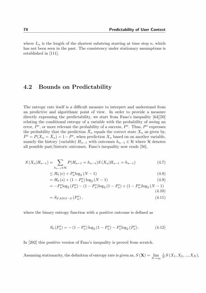
74 Predictability of User Context
where Ln is the length of the shortest substring starting at time step n, whichhas not been seen in the past. The consistency under stationary assumptions isestablished in [111].
4.2 Bounds on Predictability
The entropy rate itself is a difficult measure to interpret and understand froman predictive and algorithmic point of view. In order to provide a measuredirectly expressing the predictability, we start from Fano’s inequality [64][50]relating the conditional entropy of a variable with the probability of seeing anerror, P e, or more relevant the probability of a success, P s. Thus, P s expressesthe probability that the prediction Xn equals the correct state Xn as given by,P s = P (Xn = Xn) = 1−P e, when prediction Xn based on on another variable,namely the history (variable) Hn−1 with outcomes hn−1 ∈ H where H denotesall possible past/historic outcomes. Fano’s inequality now reads [50],
S (Xn|Hn−1) =∑
hn−1∈HP (Hn−1 = hn−1)S (Xn|Hn−1 = hn−1) (4.7)
≤ Hb (e) + P enlog2 (N − 1) (4.8)
= Hb (s) + (1− P sn) log2 (N − 1) (4.9)
= −P snlog2 (P sn)− (1− P sn)log2 (1− P sn) + (1− P sn)log2 (N − 1)(4.10)
= SFANO−S (P sn) , (4.11)
where the binary entropy function with a positive outcome is defined as
Sb (P sn) = − (1− P sn) log2 (1− P sn)− P snlog2 (P sn) . (4.12)
In [202] this positive version of Fano’s inequality is proved from scratch.
Assuming stationarity, the definition of entropy rate is given as, S (X) = limN→∞
1N S (X1, X2, ..., XN ),

4.2 Bounds on Predictability 75
thus
S (X) = limN→∞
1N S (X1, X2, ..., XN ) Definition of entropy rate (4.13)
= limN→∞
1N
∑n
n=0S (Xn|Hn−1) Chain rule for entropy (4.14)
≤ limN→∞
1N
∑n
n=0SFANO (P sn) Fano (4.15)
≤ SFANO−S(
limn→∞
1N
∑N
n=0P sn
)Concave (4.16)
= SFANO−S (〈P sn〉n) (4.17)
= SFANO−S (P s) . (4.18)
Thus, given the entropy rate of a process, S(X), the one-step-ahead predictabil-ity can be bounded from above by, P s, solving the following equality S (X) =SFANO−S (P s) for P s. Given the monotone behavior of SFANO−S this providesa unique solution, and can easily be found by standard numerical methods.
4.2.1 Upper Bound
Given the estimated entropy rate of the observed process, S(X)est, we may di-rectly find the upper bound on the one-step ahead predictability, P s,max, solvingEq.4.13. This upper bound is the main focus of [201][202] and contribution [A]and [B]. The interpretation of the this predictability bound should be performedwith the entropy estimation in mind, since the provided estimates defines thequality/accuracy of the bound.
4.2.2 Lower Bound
The bound proposed by [201] is the upper bound on the predictability, however,it is equally important to consider a lower bound in order to for example evaluatethe triviality of the problem, i.e., the upper bound may be close to one fortrivial/constant processes. In order to obtain such a lower bound, it a naturalchoice is to consider the simplest model adhering to the one-step-ahead setting,namely a first order Markov process. Thus, the probability of the next statebeing r is given by a transition probability Prs = P (Xn+1 = r|Xn = s)
P (Xn+1 = r) =∑
r∈RPrsP (Xn = s)

76 Predictability of User Context
The entropy rate of this process is given in closed form as
S (X) = −∑n
∑j
µiPij logPij , where µj is the stationary distribution of the pro-
cess which can be found by solving the following equations, µj =∑µiPij ∀ j.
Thus, given the general bound in Eq. 4.13-4.18, it is possible to find the maxi-mum predictability given this simple model. However, this is still a bound anda more direct measure is the actual predictability of this minimally complexmodel, i.e., the actual percentage of correctly classified states. This was ap-plied in [A] where classification is based on standard maximum likelihood, i.e.,arg max
rPrs (Xn+1 = r|Xn = s).
With the lower bound in place, it is possible to compare the lower and upperbound for the given process, X. In combination with the measure of predictiveinformation in Sec. 4.1, this indicates the real gain in applying a more advancedpredictive models compared to the simpler one and effectively determines theoperating range of any sensible algorithms.
4.3 Summary
The information theoretical view on predictability provides a relatively simpleand easy way to obtain bounds on the one-step-ahead predictability of discretetime series. These bounds can then be applied in engineering systems for e.g.resource allocation or in information processing systems as outlined in Chap-ter 1 for providing context aware systems or for characterizing users by theirpredictability.

Chapter 5
Summary & Conclusion
The overall aim of the thesis was to investigate elements of the general systemdescribed in Chapter 1. The focus has been the on integration of bottom-upand top-down information eliciting and modelling of perceptual and cognitiveaspects and finally quantifying the predictability of context. The thesis first ofall contributes with a holistic and general system perspective towards the inte-gration of top-down and bottom-up for audio and music organization presentedin 1. The three focus areas, outlined in the summary report - and considered inthe contributions - each contribute with new methods and/or results relevantto the field of audio and music organization. These focus areas (and relatedcontributions) are shortly summarized and concluded individually.
Computational representation of musicThe first aspect under investigation was the integration of top-down and bottom-up views of music. To this end a general review of bottom-up audio featureswas presented in the summary report (Sec.2.2) focusing on low-level featuresand how they can be representation on a song level for use in machine learningalgorithms. The summary report further outlined how these two views canbe integrated in a single model based on probabilistic topic models. This wasdescribed in some detail (Sec.2.4) providing a natural route from the well knownmulti-modal pLSA to the multi-modal LDA model, which is evaluated in H.
In conclusion, it was found that the bottom-up representation, based on audio

78 Summary & Conclusion
feature and lyrics, was more aligned with genre based tags than personal oremotional tags. It was found that the joint representation including tags, lyricsand audio performed best in a genre and style classification task, as expected.The combination of lyrics and audio improved the classification performanceover individual audio and lyric representation.
Preference learningThe primary focus of the thesis has been the realization of a general Bayesian andmodular setup for learning and modelling preference and other cognitive aspects(such as the expressed emotion music), which supports specialized experimentalparadigms and observation types, ranging from special bounded regression andranking of objects.
The summary report provided a general overview of the realized setup andplaced the individual contribution in the general context of learning and mod-elling preference and other cognitive aspects.
• Contribution [C] proposed and realised a novel likelihood model for lettingthe user convey a degree of preference for paired comparisons. Based onsimulations on a toy problem it was concluded that learning with such asresponse is faster than a standard binary response type also under adversenoisy conditions.
• Contribution [G] proposed and derived a sparse likelihood model whichallows scaling the pairwise likelihood to larger problems. Based on bothtoy and a relatively simple real-wold data, it was concluded that the sparsemodel is an effective tool in pairwise learning by comparing it to a standardGP.
• Contribution [D] proposed to use pairwise comparisons in modelling andpredicting personal music preference, modelling this by audio feature andthe probability product kernel. The approach was evaluated on a smallthree-genre dataset, and it was concluded that the model was able topredict the preference, but that a larger dataset is required to providemore support for this claim.
• Contribution [F][E] considered the modelling and representation of ex-pressed emotion in music. The contributions demonstrated how to elicitand model such complex cognitive task in a novel and robust way us-ing the proposed setup. The contributions concluded that the resultingranking is inline with common understanding of expressed emotion, andthat the pairwise Gaussian process approach performed better or equal togeneralized linear models.
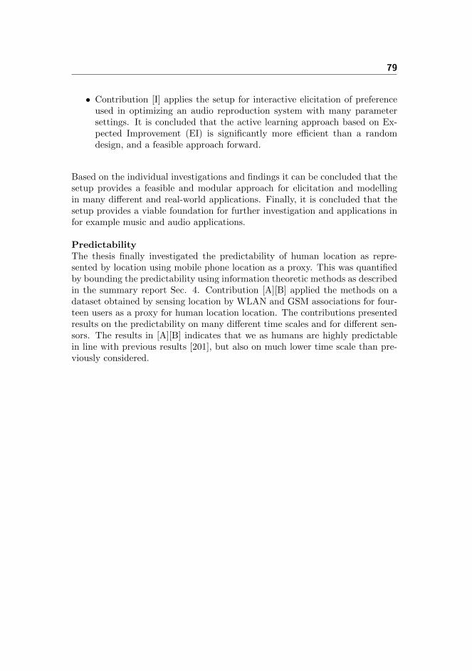
79
• Contribution [I] applies the setup for interactive elicitation of preferenceused in optimizing an audio reproduction system with many parametersettings. It is concluded that the active learning approach based on Ex-pected Improvement (EI) is significantly more efficient than a randomdesign, and a feasible approach forward.
Based on the individual investigations and findings it can be concluded that thesetup provides a feasible and modular approach for elicitation and modellingin many different and real-world applications. Finally, it is concluded that thesetup provides a viable foundation for further investigation and applications infor example music and audio applications.
PredictabilityThe thesis finally investigated the predictability of human location as repre-sented by location using mobile phone location as a proxy. This was quantifiedby bounding the predictability using information theoretic methods as describedin the summary report Sec. 4. Contribution [A][B] applied the methods on adataset obtained by sensing location by WLAN and GSM associations for four-teen users as a proxy for human location location. The contributions presentedresults on the predictability on many different time scales and for different sen-sors. The results in [A][B] indicates that we as humans are highly predictablein line with previous results [201], but also on much lower time scale than pre-viously considered.

80 Summary & Conclusion

Appendix A
Estimating HumanPredictability from Mobile
Sensor Data
Bjørn Sand Jensen, Jakob Eg Larsen, Kristian Jensen, Jan Larsen and LarsKai Hansen, Estimating Human Predictability from Mobile Sensor Data, IEEEInternational Workshop on Machine Learning for Signal Processing 2010.

82 Appendix A

ESTIMATING HUMAN PREDICTABILITY FROM MOBILE SENSOR DATA
Bjørn Sand Jensen, Jakob Eg Larsen, Kristian Jensen, Jan Larsen and Lars Kai Hansen
Technical University of Denmark,
Department of Informatics and Mathematical Modeling,
2800 Lyngby, Denmark
ABSTRACT
Quantification of human behavior is of prime interest in
many applications ranging from behavioral science to prac-
tical applications like GSM resource planning and context-
aware services. As proxies for humans, we apply multi-
ple mobile phone sensors all conveying information about
human behavior. Using a recent, information theoretic ap-
proach it is demonstrated that the trajectories of individual
sensors are highly predictable given complete knowledge of
the infinite past. We suggest using a new approach to time
scale selection which demonstrates that participants have
even higher predictability of non-trivial behavior on smaller
timer scale than previously considered.
1. INTRODUCTION
How predictable are human whereabouts? Very. At least ac-
cording to a recent study by Song et al. [1][2] based on the
predictability of location trajectories. When including the
full history of the participants, the upper bound for predic-
tion the next location lie in the 93 % range based on 45.000
participants. Song et al. use an information theoretic ap-
proach and by the use of Fano’s inequality they show [2]
that the entropy rate transforms into an upper bound of the
predictability.
The study in [1] is, however, not the first study on hu-
man predictability using mobile phones as sensors and the
area of mobile phone computing have received considerable
attention recently (see e.g. [3]). Of interest to the present
study is Eagle et al. [4], who have made extensive stud-
ies based on the Reality Mining dataset. Using a Hidden
Markov model and the time of day they show prediction ac-
curacies (home, work, elsewhere) in the range of 95 %. Us-
ing principle component analysis they furthermore analyze
the temporal patters extracted as the eigenvectors showing
clear temporal patters in daily life. Similar results have been
found by Farrahi et al. [5] by analyzing the same dataset us-
ing unsupervised methods such as LDA [5] also with the
purpose to extract patterns in everyday life.
While Eagle and Farrahi et al. use explicit modeling of
the data and extract concrete patters, Song et al. provide a
estimation of the information content using non-parametric
methods altogether resulting in the upper and lower pre-
dictability bounds of the participant behavior. We refer to
Bialek et al. [6] for further discussion on information com-
plexity in parametric and non-parametric models.
In this paper we apply a similar information theoretic
approach as in [1] to the problem of human predictability. In
comparison, we analyze a smaller but more detailed mobile
phone based dataset. This means fewer participants, similar
time span, but considerably more mobile phone sensors and
in particular higher temporal resolution.
Our goal is twofold: The possibility to analyze multi-
ple sensors is quite unique and will provide valuable insight
into the predictability of each unique sensor. The combina-
tion of sensors will furthermore convey considerably more
information about location than e.g. a GSM cell alone [1].
We show that the location and proximity based sensors all
have relatively high predictability for the entire population.
Whereas Song et al. provide important results on location
prediction, the multiple sensors in our scenario can poten-
tially provide a much richer description of context in gen-
eral. If the extended set of sensors share the predictability
of GSM cell location they may contribute additional useful
information.
Secondly, we present extended results of predictability
on different time scales which indicate that it is possible to
predict non-trivial behavior on much smaller scales than the
hour based prediction considered in [1]. In addition, we
suggest applying mutual information - or prediction infor-
mation [6] - as a method to easily estimate the optimal scale
in a non-parametric fashion.
2. MOBILE DATA
We start out describing the experimental setup underlying
the so-called lifelog dataset obtained and used in the further
analysis.
In the experiment standard Nokia N95 8GB mobile pho-
nes were used to collect data from embedded sensors in-
cluding accelerometer, GSM, GPS, Bluetooth, WLAN, and
phone activity (calls and messages) as shown in Table 1.
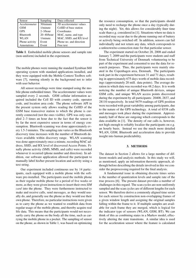
Sensor Sampling Data collected
Accelerometer 30/minute 3D accelerometer values
GSM 1/minute CellID of base station
GPS 2–3/hour Coordinates
Bluetooth 20–40/hour MAC, name, and type
WLAN 1/minute MAC, SSID, and RX level
Phone activity Event Phone no. and direction
Annotations Event Free text
Table 1. Embedded mobile phone sensors and sample rate
(non-uniform) included in the experiment.
The mobile phones were running the standard Symbian S60
operating system with standard applications installed, and
they were equipped with the Mobile Context Toolbox soft-
ware [7], running silently in the background not to infer
with user behavior.
All sensor recordings were time stamped using the mo-
bile phone embedded timer. The accelerometer values were
sampled every 2 seconds. GSM cellular information ac-
quired included the Cell ID with country code, operator
code, and location area code. The phone software API in
the present system only allows reading the CellID of the
GSM base transceiver station to which the phone is cur-
rently connected (not the ones visible). GPS was only sam-
pled 2–3 times an hour due to the fact that the sensor is
by far the most expensive sensor in terms of energy con-
sumption. Bluetooth scanning was done approximately ev-
ery 1.5-3 minutes. The sampling rate varies as the Bluetooth
discovery time increases with the number of Bluetooth de-
vices available within discovery range. WLAN scanning
was done approximately once a minute, recording MAC ad-
dress, SSID, and RX level of discovered Access Points. Fi-
nally phone activity (SMS, MMS, and calls) were recorded
whenever it occurred (phone number and direction). In ad-
dition, our software application allowed the participant to
manually label his/her present location and activity using a
text string.
Our experiment included continuous use by 14 partic-
ipants, each equipped with a mobile phone with the soft-
ware pre-installed. The participants used the mobile phone
as their regular mobile phone for a period of five weeks or
more, as they were given instructions to insert their own SIM
card into the phone. They were furthermore instructed to
make and receive calls, send messages, as they would usu-
ally do, and generally use the phone as they would use their
own phone. Therefore, no particular instructions were given
as to carry the phone as we wanted to establish data from
regular usage of the mobile phone, and thereby acquire real
life data. This means that the participants would not neces-
sarily carry the phone on the body all the time, such as car-
rying the mobile phone in a pocket. The sampling of sensor
on the phone, as shown in Table 1, was based on optimizing
the resource consumption, so that the participants should
only need to recharge the phone once a day (typically dur-
ing the night). Yet, this allows for considerably finer time
scale than e.g. considered in [1]. Situations where no data is
recorded may occur due to the phone running out of battery
or actively being switched off. In addition, sensors can fail
individually and not return any data, which corresponds to
a unknown/no-connection state for that particular sensor.
The experiment started on October 28, 2008 and ended
January 7, 2009 and the participants were students and staff
from Technical University of Denmark volunteering to be
part of the experiment and consented to use the data for re-
search purposes. Thus, the participants were mainly situ-
ated in the Copenhagen area, Denmark. The participants
took part in the experiment between 31 and 71 days, result-
ing in approximately 675 days worth of mobile data record-
ings (approximately 20 mill. data points). The average du-
ration in which data was recorded was 48.2 days. It is worth
noticing the number of unique Bluetooth devices, unique
GSM cells, and unique WLAN access points discovered
during the experiment by all participants: 20408, 2837, and
28110 respectively. In total 9479 readings of GPS position
were recorded with great variability among participants, due
to the nature of the GPS technology. A total of 6538 calls
and messages took place during the experiment. Approxi-
mately half of these are outgoing which corresponds to the
data available in [1]. The density of our calls is, however,
not high enough to reliably localize the participants on e.g.
an hourly basis. Instead we use the much more detailed
WLAN, GSM, Bluetooth and acceleration data to provide
insight into human predictability.
3. METHODS
The dataset in Section 2 allows for a large number of dif-
ferent models and analysis methods. In this study we will,
as mentioned, apply an information theoretic approach, al-
though before describing the details involved in this we con-
sider the preprocessing required for the final analysis.
A fundamental issue in obtaining discrete times series
is the number of quantization levels and sample rate of the
true process [6]. The present dataset provides a number of
challenges in this regard. The scan cycles are non-uniformly
sampled and the scan cycles are of different lengths for each
sensor. We therefore derive a commonly aligned time series
for each sensor by construction non-overlapping frames of
a given window length and assigning the original samples
falling within the frame to it. If multiple samples are avail-
able for each frame they are merged, which is logical for
the indicator type of sensors (WLAN, GSM, BT). We can
think of this as combining states in a Markov model, effec-
tively altering the state transitions. A similar idea is used
for the acceleration sensor where the feature is calculated

W1
W2
W3
W4
W5
W6
W7
W8
W9
W10
W11
Mon* Tue Tue* Wed Wed* Thu Thu* Fri Fri* Sat Sat* Sun
Fig. 1. Participant 1’s GSM data for 11 weeks, with * de-
noting noon. The figure shows the top 20 most visited GSM
cell towers as rows in each week. The time series is con-
sidered in a vector space representation, hence each unique
column corresponds to a state.
as the average power within a window represented as a dis-
crete levels, i.e. XACC ∈ {off, 1, 2, 3}. For example, us-
ing the WLAN and integrating all the nets seen into a state
effectively means that the predictive variable becomes the
WLAN state and not the location as such. If a location is
required we could lookup the WLANs positions and gener-
ate a location variable from that. The alternative choice of
directly working on a location variable generated from the
WLANs is not considered here.
The proposed representation is a very detailed descrip-
tion of the participant state. On the contrary the alternative,
as used in [1] [2], suggest using only the location (GSM
cell) seen the most within a time window as the state. Both
methods involve a quite complex quantization of the origi-
nal data into windows. To evaluate the consequence of this
on predictability we consider the change in predictability
bounds as the window length is increased from one minute
to one hour based on the GSM series.
3.1. Information Theoretic Measures
We consider the task of quantifying the predictability possi-
ble in our discrete time series, X = (X1, X2, .., Xn), where
n is the time index. This is largely inspired by previous
work on predictability, complexity and learning (see e.g.
[6]) on dynamical systems, and the recent development on
a similar dataset as ours [1]. Here predictability quantifies
the probability of an algorithm correctly predicting the next
state. Thus, given the history the fundamental distribution
of interest is P (Xn+1|X1, X2, .., Xn). In the case where
we have no information regarding the past the distribution
reduces to P (X). When P (X) is uniform, i.e. each of Nstates have the same probability, the Shannon entropy (in
bits) is defined as Hrand (X) = log2 N .
If, however, the distribution of X is non-uniform, the
entropy is given as Hunc (X) = −∑i∈I p (xi) log (p (xi)),
with p (x) = P (X = x). We use a maximum likelihood
plug-in estimate of p(x). This in turn represents the infor-
mation when no history is available, hence the acronym unc
(uncorrelated).
The true entropy of the participant, or the average num-
ber of bits needed to encode the symbols in the sequence,
can be estimated taking into account the infinite history.
Formally this the done by defining the stationary stochas-
tic process X = {Xi} which have the entropy rate given by
H (X) = limn→∞
1n
∑ni=1 H
(Xi|hi−1
), where the history hi
at time step i is hi = {X1, X2, ..., Xi−1}. In our case it is
noted that 0 ≤ H ≤ Hunc ≤ Hrand < ∞.
An appealing aspect of these non-parametric methods
is that we avoid directly limiting model complexity as in
any parametric or semi-parametric models. However, a ma-
jor challenge in using these information measures based on
real and unknown processes is the estimation of the entropy
rate. A number of ideas have emerged based on compres-
sion techniques such as Lempel-Ziv (LZ) (including string
matching methods) and Context Weighted Trees (we refer
to [8] for an overview). In this study we estimate the en-
tropy rate using the efficient and fast converging LZ based
estimator as described in [9][8] and also applied in [2]. The
LZ based estimate for a time series of length n is given by
Hest =[1n
∑ni=1
Li
log2n
]−1
, where Li is the shortest sub-
string starting at time step i, which has not been seen in
the past. The consistency under stationary assumptions is
proved in [9] where it is applied to English text.
Given estimates of the entropy and the entropy rate we
consider a related quantity, namely mutual information - or
predictive information [6] - defined using the information
measures above.
Ipred = limn→∞
1
n
n∑
i=1
H (Xi)−H(Xi|hi−1
)(1)
= Hunc (X)−Hest (X) (2)
Ipred represents the mutual information between the distri-
butions corresponding to knowing and not knowing the past
history. That is, it quantifies the fundamental information
gain in knowing the (complete) past when prediction the
future and we propose it as a way to evaluate optimal quan-
tization and time scale selection. We illustrate the behavior
of the measure on a time scale selection problem.

3.2. Predictability Bounds
We consider the probability, Π, that an arbitrary algorithm
is able to predict the next state correctly.
Based on the entropy rate and Fano’s inequality Song et
al. derive a bound so Π ≤ Πmax (H (X) , N) with Πmax
given by the relation H (Πmax) = −Πmaxlog2 (Πmax)−
(1−Πmax) log2 (1−Πmax) + (1−Πmax) log2 (N − 1).This non-linear relation between Πmax and the estimate of
H(X) is easily solved using standard methods (see [2] for
a full derivation). .
By applying this approach we obtain three upper bounds
based on the entropy estimates previously mentioned. The
first, Πrand, provides an upper bound on a random predic-
tor. The second upper bound is Πunc which bounds the per-
formance obtainable with a predictor utilizing the state dis-
tribution. Finally, the most interesting bound, Πmax, pro-
vides a upper limit for the performance of any predictor uti-
lizing the infinite past.
Equally interesting as the upper bound is a lower bound
on the predictability, i.e. the worst we can expect from any
predictor. Song et. al. shows how a simple lower bound
can be constructed based on the so-called regularity. The
regularity is in essence a simple predictor based on the most
likely situation given the time of day. This is an intuitive
measure for some time periods such as daily patters, e.g.
utilizing where a person is most likely to be each morning
at 6.00. However, if the time scale is in the minute range it
does not necessarily make sense to consider the regularity.
We propose instead to use a predictor using the imme-
diate past as the representative of the lower predictability
bound. Hence, we select a first order Markov model with
the transition probabilities estimated from our finite process.
For generalization purposes we use a resampling scheme
in which the entropy and the next state distribution is esti-
mated based on 2/3 of the data and tested on the remaining
1/3. This is performed for nine repetitions in a compromise
between accuracy of the generalization estimate and the re-
quired samples in order for the entropy estimator to con-
verge. The resampling further allows us to verify that the
LZ entropy estimate converges to reasonable similar values
for separate temporal sections of the participants life. Any
variation over sections will result in a greater variance of the
predictability.
3.3. Missing data
Missing data constitutes a major issue in applying mobile
phones as proxies for human behavior. Our dataset contains
two types of missing data: A well-defined off-state and a
state where an individual sensor is off/disconnected. The
current dataset does not provide any option to differentiate
the latter case from not being in range of e.g. any Bluetooth
devices, and will consequently be treated as the same state.
We can either predict the true off-state or simply ignore
it. Based on initial studies it was found that the convergence
of the entropy estimate was more consistent when not in-
cluding the off-state and instead representing off-states by a
single terminal symbol in the LZ based estimation.
An alternative suggested by Song et al. [1] provide an
ad-hoc method for extrapolating the entropy corresponding
to a missing data fraction, q, of zero. They show empir-
ically that the ratio ln (Hest/Hunc) has a linear relation-
ship across a wide range of missing data fractions. Unfor-
tunately we are not able to obtain such a linear relationship
in our data set except for four participants. When extrap-
olated, these participants show precision within ≤10 % for
q = [0; 0.5], however, the majority, of participants (ten) de-
viates with ≫10%, which is not found acceptable for our
study.
4. EXPERIMENTAL RESULTS
We apply the methods described in Section 3 and illustrate
the potential predictability by analyzing the GSM, WLAN,
BT and acceleration data, described in Section 2. From the
results of the 14 participants we estimate the probability
density function using a standard kernel density estimator
with fixed width for each density across all experiments.
4.1. Sensors
Initially we consider the estimated predictability bounds com-
paring individual sensors at the same time scale, specifically
15 minutes. Fig. 2 shows the predictability bounds of the
GSM, WLAN, BT and activity variables. By examining
the difference between Πmax and Πunc we find that there is
considerable gain in knowing the past. From the difference
between the Markov model ΠMarkov and the upper bound,
ΠMax, we see that knowing more than just the previous state
seems on average to provide considerable benefit.
In the uncorrelated model participants show consider-
able differences in the entropy, Hunc, for all sensors as
typically expected in a real population. However, condi-
tioned on the past, the variability is typically lower (except
for WLAN), indicating that on average, participants with
high entropy have a relative predictable trajectory. This
corresponds well with the results observed in [1] for GSM
based localization. The Bluetooth data does, as mentioned,
contain a considerable fraction of unknown states (not off-
states), which will tend to underestimate the true entropy.
This means that the bounds are most likely overestimated
for Bluetooth.
The GSM, WLAN and Bluetooth sensors are inherently
location or proximity oriented sensors, and the estimated
distributions all have modes in the high range above 80%,
but with noticeable difference in variability. Whereas GSM

Fig. 2. GSM, WLAN and Acceleration. Crosses indicate
individual participant estimates.
provides small variability among participants, WLAN seems
to provide a much larger difference among participants. This
is not surprising since WLAN is considerably more noisy
than GSM and captures a more local and detailed state than
GSM. Thus, some participants tend to have a relatively low
predictability while others are just as predictable as using
GSM. The GSM complexity is more similar between mo-
bile phone users. Thus, the WLAN sensor will probably
provide the more interesting data, but it is the harder sensor
to predict. At least when using the very detailed representa-
tion.
In order to do a preliminary analysis of the information
shared between the sensors, we consider the averaged nor-
malized mutual information (not conditioned on the past) in
Table 2. We generally see that the location/proximity driven
sensors show some redundancy as expected, while the activ-
ity seems to provide a different element of human behavior.
4.2. Time Scale
Fig. 4 shows the effect of varying the window length from
one hour to one minutes for the GSM sensor given the state
representation described in 3. In doing so, we note that
the number of states reduces (see Πrand). From Fig. 4 we
find that the increase in window length towards 3600 sec-
Fig. 3. GSM predictability vs. window length in sec. (log
scale). The density estimate of Πrand is removed for clar-
ity. Participant 3 is furthermore removed for clarity due to
his/her outlier nature.
onds tends to remove the correlation effectively rendering
the process more random seen by the decrease in estimated
predictability. It should be noted that the behavior of these
time selection graphs are highly influenced by the repre-
sentation applied, i.e. the way the different series are con-
structed (see Section 3).
An important point to emphasize, is the fact that the in-
creased predictability is not only an effect of a trivial behav-
ior (i.e. constant). This would imply that the markov model
would perform nearly as good as the upper bound suggests.
Hence, the increase in predictability can actually be used
to predict a non-trivial behavior, and improve for example
context-aware applications.
In examining the predictive information Fig. 2 we find
an optimal window of approx. 4-5 minutes. Hence, this is
the point where we obtain the highest gain in knowing the
infinite past when predicting the future. We note that the
simpler Markov model actually continues to improve as the
window length decreases. This indicates that the process
becomes more and more trivial (although not completely)
and the gain decreases at the very lowest window length.
GSM WLAN BT ACC
GSM 1.00 0.45 (0.17) 0.42 (0.14) 0.07 (0.02)
WLAN 1.00 0.55 (0.17) 0.10 (0.03)
BT 1.0 0.08 (0.05)
ACC 1.00
Table 2. Average, normalized mutual information and stan-
dard deviation across participants. Normalization is per-
formed as I (X ;Y ) /max {H (X) , H (Y )}.

60 120 300 600 900 1800 270036000.55
0.6
0.65
0.7
0.75
0.8
0.85
0.9
0.95
1
Window (sec)
Ipre
d
Average Ipred
Individual Ipred
Fig. 4. Predictive Information (normalized) vs. window
length (log scale). Dashed blue graphs: individual partici-
pants. Black graphs: participant mean and std. deviation.
Therefore, we aim for the time scale with some non-trivial,
but predictable behavior.
For direct comparison with the results in [1] we refer to
the one hour window in Fig. 4. We find that the estimated
bound and distribution is in the same range. However, the
datasets are inherently different and our results suggest a
slightly lower predictability with higher variability between
users at this time scale. Overall, though, our results at other
times scales supports the conclusion that human trajectories
on GSM cell scale are indeed very predictable despite the
apparent difference in the number of visited states.
5. DISCUSSION
A major issue in the method proposed by Song et al. [2] is
the quality (bias/variance) and convergence of the entropy
estimator, which is not addressed in [1]. Secondly, the as-
sumed stationarity does not per default apply to all partici-
pants, hence quantifying the effect on the entropy estimate
is of vital importance. In order to provide reliable results,
we have verified a reasonable convergence on the individual
subsections, however, the reported upper bound should only
be considered a rough estimate. Future work will attempt to
improve the apparent issues using the entropy estimate.
An obvious extension of the current analysis is evalua-
tion of sensor combinations. However, computing e.g. the
mutual information conditioned on the past is rendered diffi-
cult by the present lack of statistics for the LZ based entropy
estimator.
6. CONCLUSION
In this study we presented a new dataset offering vast possi-
bilities of modeling human behavior. In this initial analysis
we adopted an implicit modeling approach based on infor-
mation theoretic methods to provide bounds for the perfor-
mance potentially obtainable using explicit modeling.
We presented novel results on the predictability of mul-
tiple mobile phone sensors, showing that the findings in [1]
generalizes to many more location based sensors. This out-
lines interesting potential for future context-aware mobile
services and applications.
Finally, we showed that the prediction of human mo-
bility is not limited to the one hour time scale previously
studied. In particular, we find that predictability seems to
further improve at time scales down to about 4-5 minutes.
7. REFERENCES
[1] Chaoming Song, Zehui Qu, Nicholas Blumm, and
Albert-Laszlo Barabasi, “Limits of predictability in hu-
man mobility,” Science, vol. 327, no. 5968, pp. 1018–
1021, 2010.
[2] Chaoming Song, Zehui Qu, Nicholas Blumm, and
Albert-Laszlo Barabasi, “Limits of predictability in hu-
man mobility - supplementary material,” 2010.
[3] Roberta Kwok, “Personal technology: Phoning in
data.,” Nature, vol. 458, no. 7241, pp. 959–961, 2009.
[4] Nathan Eagle and Alex (Sandy) Pentland, “Reality min-
ing: sensing complex social systems,” Personal and
Ubiquitous Computing, vol. 10, no. 4, pp. 255–268,
2006.
[5] Katayoun Farrahi and Daniel Gatica-Perez, “Learning
and predicting multimodal daily life patterns from cell
phones,” in Proceedings of the 2009 international con-
ference on Multimodal interfaces, 2009, pp. 277–280.
[6] William Bialek, Ilya Nemenman, and Naftali Tishby,
“Predictability, complexity, and learning,” Neural Com-
put., vol. 13, no. 11, pp. 2409–2463, 2001.
[7] Jakob Eg Larsen and Kristian Jensen, “Mobile con-
text toolbox - an extensible context framework for s60
mobile phones,” in Proceedings of the 4th European
Conference on Smart Sensing and Context (EuroSSC),
2009.
[8] Yun Gao, Ioannis Kontoyiannis, and Elie Bienenstock,
“Estimating the entropy of binary time series: Method-
ology, some theory and a simulation study,” Entropy,
vol. 10, no. 2, pp. 71–99, 2008.
[9] I. Kontoyiannis, P.H. Algoet, Yu M. Suhov, and A.J.
Wyner, “Nonparametric entropy estimation for station-
ary process and random fields, with applications to en-
glish text,” IEEE Transactions on Information Theory,
vol. 44, no. 3, pp. 1319–1327, 1998.

Appendix B
Predictability of MobilePhone Associations
Bjørn Sand Jensen, Jan Larsen, Kristian Jensen, Jakob Eg Larsen, and LarsKai Hansen, Predictability of Mobile Phone Associations, European Conferenceon Machine Learning : Mining Ubiquitous and Social Environments Workshop,2010.

90 Appendix B
PREDICTABILITY OF MOBILE PHONE
ASSOCIATIONS
Bjørn Sand Jensen, Jan Larsen, Kristian Jensen,Jakob Eg Larsen, and Lars Kai Hansen
Technical University of Denmark{bjje,jl,krije,jel,lkh}@imm.dtu.dk
Abstract. Prediction and understanding of human behavior is of highimportance in many modern applications and research areas ranging fromcontext-aware services, wireless resource allocation to social sciences. Inthis study we collect a novel dataset using standard mobile phones andanalyze how the predictability of mobile sensors, acting as proxies for hu-mans, change with time scale and sensor type such as GSM and WLAN.Applying recent information theoretic methods, it is demonstrated thatan upper bound on predictability is relatively high for all sensors giventhe complete history (typically above 90%). The relation between timescale and the predictability bound is examined for GSM and WLANsensors, and both are found to have predictable and non-trivial behavioreven on quite short time scales. The analysis provides valuable insightinto aspects such as time scale and spatial quantization, state representa-tion, and general behavior. This is of vital interest in the development ofcontext-aware services which rely on forecasting based on mobile phonesensors.
1 Introduction
The wide acceptance of sensor rich mobile phones and related applications en-ables deep studies of human behavior. According to a recent study by Song etal. [11, 12] based on mobile phone location trajectories, individual human mo-bility patterns are highly predictable. When including the complete history ofthe participants they derived an upper bound on prediction of the next locationof 93% in a large cohort of 45,000 users. The upper bound is based on informa-tion theory. Using Fanos inequality it was shown in [12] that the entropy ratetransforms into an upper bound of the predictability.
Interest in understanding human behavior using mobile technology is increas-ing, see e.g., the recent review by Kwok [9]. The work of Eagle et al. [4] on theReality Mining dataset, marks an early and important contribution. Using aHidden Markov model and the time of day, they demonstrate explicit predictionaccuracies (home, work, elsewhere) in the order of 95%. Furthermore, they useprinciple component analysis (PCA) to visualize temporal patterns in daily life.The stability of these temporal patterns was confirmed by Farrahi et al. [5] inthe same dataset using unsupervised topic models.

While Eagle et al. focus on finding statistical regularities in behaviors at thegroup level using parametric models Song et al. [11] are interested in individualpredictability using non-parametric methods and argue that inter-participantvariability is significant and in fact power-law distributed. For a further discus-sion on parametric and non-parametric models, and the relation to informationtheory, we refer to Bialek et al. [3].
We follow the implicit modeling approach by Song et al., i.e., using boundsrather than explicit predictors to discuss human behavior in a novel mobilephone data set that complements the analysis of Song et al. Our data set hassignificantly higher temporal resolution and involves more sensors, however, ina much smaller cohort (N = 14).
The opportunity to analyze multiple sensors is quite unique and produces newinsight both on the predictability of each sensor and on sensor dependencies. Weshow that all the location and proximity based sensors have a relatively highpredictability bounds for the entire population. Whereas Song et al. [11] provideimportant results on location prediction, the multiple sensors applied in ourstudy can potentially provide a richer description of context beyond location.And as the extended set of sensors enjoys similar high predictability rates, itmay contribute additional useful information on human behavior and supportmore general context dependent services.
Furthermore, we are interested in the predictability on different time scales,and to probe whether it is possible to predict non-trivial behaviors on smallerscales than the one hour time scale considered in [11]. Finally, we suggest apply-ing mutual information - or prediction information [3] - as a method to easilyestimate an optimal time scale in a non-parametric fashion. The informationtheoretic approach is based on upper and lower bounds on predictability. In thispaper we use the upper bound proposed by Song et al., and derive and analyzea tighter lower bound based on a first Markov model [7], rather than the zeroorder model of [12].
An early version of this work was presented to the machine learning commu-nity in [7]. The present paper extends this work with; 1) an extended descriptionof the experimental setup; 2) comparison between WLAN and GSM, in particu-lar in relation to optimal time scale; 3) extended discussion and interpretation.
The paper first gives a presentation of the experimental setup and the ac-quired mobile phone dataset. In Section 3 we present the information theoretictools necessary to follow the analysis of the dataset. The result of the study ispresented and discussed in Section 4, followed by the conclusion in Section 5.
2 Experimental Setup
Within the last decade there has been a number of studies of real-world dataset orlifelogs reflecting human life [1, 2]. In this section we present a software platformfor obtaining such lifelogs using standard off-the-shelf mobile phones functioningas individual wearable sensor platforms.

Fig. 1. Mobile Context Toolbox architecture [10]. The bottom two layers provide low-level access to the embedded sensors, whereas the adapters and context widget layersprovide high-level Python interfaces to sensors and inferred information for applica-tions.
2.1 Mobile Context Toolbox
Since utilizing multiple sensor inputs on mobile devices can be a complex task wehave used our Mobile Context Toolbox [10], which provides an open extensibleframework for the Nokia S60 platform running the Symbian mobile OperatingSystem present in mobiles phones such as Nokia N95. The framework providesaccess to multiple embedded mobile phone sensors, including accelerometer, mi-crophone, camera, etc., as well as networking components such as phone appli-cation data (calendar, address book, phone log, etc.), and phone state (profile,charge level, etc.).
In principle, mobile devices can acquire information from the surroundingenvironment as well as from online sources, but in the present study we focus oninformation that can be acquired through the large variety of sensors embeddedin the device. The framework has multiple layers (as depicted in Fig. 1) on top ofthe Nokia S60 platform. The framework uses Python for S60 (PyS60) with a setof extensions for accessing low-level sensors and application data. The adapterslayer provides interfaces for the low-level sensors, whereas the context widgetsuses one or more adapters to infer higher-level contextual information. Finally,
the application layer utilize contextual information inferred from context widgetsand/or directly from context adapters. Further details and explanation of theMobile Context Toolbox is provided in [10].
2.2 Logging Data From Embedded Sensors
For the purpose of using mobile phones as an instrument for gathering lifeloginformation we have built a Context Logger application, which subscribes to allsensors through the relevant system components and then continuously recordsall events received from the multiple adapters and widgets. In effect all accessiblesensor data is recorded, as shown in Table 1.
All sensor recordings are time stamped using the embedded mobile phonetimer. The accelerometer was sampled every 2 seconds. Samples are read-outevery 30s, in batches of 15 samples. The purpose of reading in bursts is to en-able reading short bursts with higher sampling rate. GSM cellular informationacquired included the Cell ID with country code, operator code, and locationarea code. In the present system the phone software API only allow reading theCellID of the GSM base transceiver station to which the phone is currently con-nected (not the ones visible). Since the GPS sensor is the most energy expensivesensor, it was only sampled 2–3 times an hour to reduce the energy consump-tion. Bluetooth scans was performed approximately every 1.5-3 minutes. Thesampling rate varies as the Bluetooth discovery time increases with the numberof Bluetooth devices available within discovery range. A discovery of a Bluetoothdevice will always produce the unique MAC address of the device, however, thelookup of the Bluetooth ”friendly name” and device type might fail as more timeis required to obtain this information. WLAN scanning is performed approxi-mately once a minute, recording MAC address, SSID, and RX level (power ratioin decibels – a measurement of the link quality) of discovered Access Points. Fi-nally, phone activity (SMS, MMS, and calls) were recorded whenever it occurred(phone number and direction).
In addition to the above mentioned sensor data, the Context Logger applica-tion allows a user to manually label his/her present location and activity. Thelabel is a text string which can be entered by the user on the mobile phone,such as, home, running, and having dinner. Entered labels will be stored andsubsequently shown on a list to pick from in order to avoid re-typing locationand activity labels. Users can manually choose to label location and activity by
Sensor Sampling Data
Accelerometer 30/minute 3D Accelerometer valuesGSM 1/minute CellID of GSM base transceiver stationGPS 2–3/hour Longitude, Latitude, and AltitudeBluetooth 20–40/hour Bluetooth MAC, friendly name, and device typeWLAN 1/minute Access Point MAC address, SSID, and RX levelPhone activity Event Phone number and direction of call or messageTable 1. List of embedded mobile phone sensors used for collecting data

selecting a menu item in the Context Logger application, however, this mech-anism is further enhanced with the ability to automatically prompt for labels.Thus, a user can choose to enter a label at any point in time, but the applicationwill also prompt the user to label a location and activity 2–3 times a day in orderto receive feedback. The data location and activity data recorded on the mobilephone is a key-value pair along with the time stamp. There are no pre-definedlocation and activity labels defined in the application and the labeling is com-pletely free form with the users determining, how they want to write their textlabels.
Situations with missing data may occur due to the phone running out ofbattery, being switched off, or simply not able to acquire data through one ormore sensors (for instance no GSM reception).
2.3 Data Collection
An initial deployment of the system included continuous use by 14 participants,each equipped with a standard mobile phone (Nokia N95) which had the MobileContext Toolbox pre-installed along with the Context Logger application thatwould continuously record the data acquired from all sensors currently supportedby our framework. The participants were using the mobile phone as their regularmobile phone for a period of five weeks or more, as they were given instructionsto insert their own simcard into the phone. Furthermore, they were instructedto make and receive calls, send messages, etc., as they would usually do, andgenerally use the phone as they would use their own phone. Therefore, no par-ticular instructions were given, since we wanted to establish data from regularusage of the mobile phone, and thereby acquire real-life data. This means thatthe participants would not necessarily carry the phone on the body all the timesuch as carrying the mobile phone in a pocket.
As the survey is completely dependent on the cooperation of the participantsand due to increased use of sensors, the lack of battery time was considered arisk in terms of participants leaving the survey. Thus, the sensor configurationof sampling on the phone was based on optimizing the resource consumption,so that the participants should only need to recharge the phone once a day(typically during the night).
The experiment started on October 28, 2008 and ended January 7, 2009 andthe participants were students and staff members from The Technical Universityof Denmark volunteering to be part of the experiment. Thus, the participantswere mainly situated in the greater Copenhagen area, Denmark. The 14 partic-ipants took part in the experiment between 31 to 71 days, resulting in approxi-mately 472 days of data covering data collection periods totalling 676 days. Theaverage duration was 48.2 days. An overview of the collected data is provided inTable 2.
During the experiment a total of approximately 20 million data points werecollected with the accelerometer contributing the most with 14.5 million datapoints. A summary of recordings from Bluetooth scans, WLAN scans, GPSreadings, and GSM readings can be seen in Table 2. It is worth noticing the

Part. Accel BT. BT.* GPS GSM GSM* Ann. PA. WLAN WLAN* Days
1 1474480 54349 2846 516 69458 529 533 544 224101 6387 71
2 2045773 38028 2478 1514 75669 603 596 1062 364272 6040 66
3 318597 27329 790 12 37217 98 222 21 125600 630 31
4 875287 7880 743 2 17750 228 134 620 186421 2394 52
5 1117147 13575 2373 4058 56206 227 386 277 251016 2347 48
6 711490 23702 1141 95 51702 235 82 839 92396 2119 50
7 1184457 13327 1765 3 45826 955 272 581 139466 4017 46
8 700258 42346 2080 614 74250 172 212 74 154108 3359 41
9 1101926 42346 1050 119 37393 100 104 497 104576 1804 38
10 1103086 21676 2104 419 63937 419 414 116 192338 2650 48
11 1122315 12492 655 929 46158 929 163 121 295716 2286 47
12 796452 30610 2317 40 51548 40 143 151 97769 2403 50
13 1024276 27550 1741 1114 49349 1114 137 949 171951 5463 51
14 971558 21502 1303 44 40017 44 149 686 118687 1263 36
Total 14547102 350879 20408 9479 716480 2837 3547 6538 2518417 28110 48.2
Table 2.Overview of collected data for each participant in the experiment: Participant,Accelerometer, Bluetooth, Unique Bluetooth devices, GPS, GSM, Unique GSM cells,Annotations, Phone Activity, WLAN Access Points, Unique WLAN Access Points,Duration in days.
number of unique Bluetooth devices, unique GSM cells, and unique WLAN ac-cess points discovered accumulatively during the experiment by all participants:20408, 2837, and 28110, respectively. In total 9479 readings of GPS positionwere recorded, but the recordings varies a lot among the participants due to thenature of the GPS technology. As a GPS position typically can not be obtainedindoor only a subset of users have sufficient recordings of GPS position. Forinstance, if they typically place the mobile phone near a window when indoorwhere a GPS position can be obtained. A total of 6538 calls and messages tookplace during the experiment.
The participants provided 3547 annotations of locations and activities intotal. On average the participants provided 253 annotations during their par-ticipation, with an overall average of 5.3 labels provided per user per day. Themost active participants provided 8-9 labels per day on average, whereas theleast active participants provided 2 labels per day on average.
3 Methods
In this study we will apply an information theoretic approach in the analysisof the dataset obtained and described in Section 2. Although before describingthe details involved in this, we consider the preprocessing required for the finalanalysis.
A general issue in obtaining discrete times series is the number of quantizationlevels and sample rate of the true process [3]. The scan cycles used to obtain the

present dataset are non-uniformly sampled and the scan cycles are of differentlength for each sensor. We therefore construct a commonly aligned time series foreach sensor by creating non-overlapping frames of a given window length. Theoriginal samples falling within the frame is then assigned to it. If multiple samplesfalls within a frame they are merged, which is reasonable for the indicator typeof sensors (WLAN, GSM, BT). This is similar to combining states in a Markovmodel effectively altering the state transitions. In case of the acceleration sensor,the feature is calculated as the average power within a window represented asa discrete levels1, i.e., XACC ∈ {off, 1, 2, 3}. Considering the WLAN sensorand integrating all the networks seen into a state effectively means that thepredictive variable becomes the WLAN state and not the location as such. If aspecific location is needed a lookup to a database could return the position of theWLAN access point and generate a location variable from that. An alternativewould be to directly work on a location variable generated from the WLANaccess point, but this is not considered here.
The proposed representation constitutes a very detailed description of theparticipant state. An alternative suggested in [11, 12], represents the state as themost visited GSM cell location within a time window. Both approaches involve arelatively complex temporal quantization and resampling of the original data. Toevaluate the consequence temporal scale, we consider the change in predictabilitybounds as the window length is decreased from one hour to one minute.
3.1 Information Theoretic Measures
We consider the problem of quantifying the predictability obtainable in a dis-crete process, X = (X1, X2, .., Xi), where i is the time index and X is the statevariable. This is to a large degree motivated by previous work on predictabil-ity, complexity and learning (see e.g. [3]), and recent development on a similardataset [11]. Here predictability is defined as the probability of an arbitrary al-gorithm correctly predicting the next state. Hence, given the history the basicdistribution of interest is P (Xi+1|X1, X2, .., Xi). In the case where we have noinformation regarding the history, the distribution naturally reduces to P (X).When P (X) is uniform, i.e., each of M states have the same probability ofoccurring, the Shannon entropy (in bits) is defined as Hrand (X) = log2 M .
In the case where the distribution of X is non-uniform, the entropy is givenas
Hunc (X) = −∑
i∈Ip (xi) log (p (xi)) (1)
with p (x) = P (X = x). This in turn represents the information when no historyis available, hence, the acronym unc (uncorrelated).
The entropy rate of the participants trajectory, or the average number ofbits needed to encode the states in the sequence, can be estimated taking into
1 An equiprobable quantization is used, i.e., each level has the same frequency ofoccurrence within the entire dataset.
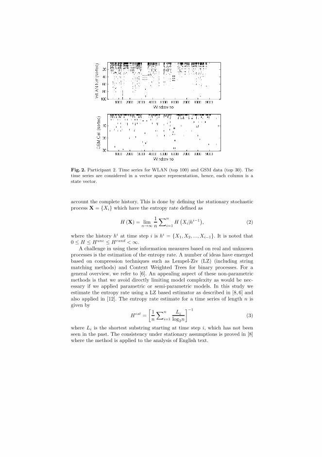
Fig. 2. Participant 2. Time series for WLAN (top 100) and GSM data (top 30). Thetime series are considered in a vector space representation, hence, each column is astate vector.
account the complete history. This is done by defining the stationary stochasticprocess X = {Xi} which have the entropy rate defined as
H (X) = limn→∞
1
n
∑n
i=1H
(Xi|hi−1
), (2)
where the history hi at time step i is hi = {X1, X2, ..., Xi−1}. It is noted that0 ≤ H ≤ Hunc ≤ Hrand < ∞.
A challenge in using these information measures based on real and unknownprocesses is the estimation of the entropy rate. A number of ideas have emergedbased on compression techniques such as Lempel-Ziv (LZ) (including stringmatching methods) and Context Weighted Trees for binary processes. For ageneral overview, we refer to [6]. An appealing aspect of these non-parametricmethods is that we avoid directly limiting model complexity as would be nec-essary if we applied parametric or semi-parametric models. In this study weestimate the entropy rate using a LZ based estimator as described in [8, 6] andalso applied in [12]. The entropy rate estimate for a time series of length n isgiven by
Hest =
[1
n
∑n
i=1
Li
log2n
]−1
(3)
where Li is the shortest substring starting at time step i, which has not beenseen in the past. The consistency under stationary assumptions is proved in [8]where the method is applied to the analysis of English text.

Given estimates of the entropy and the entropy rate we consider a relatedquantity, namely mutual information - or predictive information [3]. This mea-sure is already available given the information measures above as
Ipred = limn→∞
1
n
n∑
i=1
H (Xi)−H(Xi|hi−1
)(4)
= Hunc (X)−Hest (X) (5)
In effect Ipred represents the mutual information between the distributions cor-responding to knowing and not knowing the past history. Hence, it quantifies thefundamental information gain in knowing the (complete) past when predictionthe future, and we propose it as a easy way to evaluate quantization and timescale effects. We illustrate the behavior of the measure on a time scale selectionproblem in Section 4.
3.2 Predictability
In order to construct bounds on the predictability we consider the probability,Π , that an arbitrary algorithm is able to predict the next state correctly.
Based on the entropy rate and Fano’s inequality Song et al. derives a boundso Π ≤ Πmax (H (X) ,M) with Πmax given by the relation [12]
H (X) = H (Πmax) + (1−Πmax) log2 (M − 1) (6)
with the function, H (Πmax), given by
H (Πmax) = −Πmaxlog2 (Πmax)− (1−Πmax) log2 (1−Πmax) (7)
This non-linear relation between Πmax and the estimate ofH(X) is easily solvedusing standard methods (for a full derivation see [12]).
Adopting this approach we obtain three upper bounds based on the entropyestimates previously mentioned. The first, Πrand, provides an upper bound ona random predictor. The second upper bound is Πunc which bounds the per-formance obtainable with a predictor utilizing the observed state distribution.Finally, the most interesting bound, Πmax, provides a upper limit for the per-formance of any algorithm utilizing the complete past.
The upper bound is of course interesting in understanding the potential pre-dictability, although we find a lower bound equally important in the analysis.Song et. al. [11] show how a simple lower bound can be constructed based onthe so-called regularity. The regularity is in essence a zero order Markov modelbased on the most likely state at any given time of the day, i.e., using only thetime of occurrence and no sequence information. This is an intuitive measure forsome time periods such as daily patterns, e.g., utilizing where a person is mostlikely to be each morning at 7.00. However, if the time scale is in the minuterange it does not necessarily make sense to consider the regularity.
Instead we propose to use a predictor using the immediate past as the repre-sentative of the lower predictability bound. For this purpose we use a first order

Markov model with the transition probabilities estimated from the finite process.Thus, the next state prediction is based on the distribution P (Xi+1|X1, X1, ..., Xi) =P (Xi+1|Xi).
To avoid overfitting which tends to render the bounds overly optimistic, weuse a resampling scheme in which the entropy and the next state distributionis estimated based on 2/3 of the data and tested on the remaining 1/3. Thisis performed for nine distinct subsections in a compromise between accuracy ofthe estimate and the needed samples for the entropy estimator to converge. Theresampling further allows us to verify that the LZ entropy estimate converges toreasonable similar values for separate temporal sections of the participants life.Any variation across subsections will result in a greater variance of the estimatedbound.
4 Results
In order to provide insight into the predictability of mobile phones sensors andthereby indirectly insight into human behavior, we apply the information theo-retic methods described in Section 2. The density estimates of the bounds areall made using a standard kernel based density estimator (the bandwidth ishand-tuned for visualization).
4.1 Individual Sensors
One of the goals in this study is to analyse the potential predictability of dif-ferent sensors and to that end we provide the predictability bounds for the fourprominent sensors in the dataset, specifically GSM, WLAN, Bluetooth and ac-celeration at 15 min. window length. Fig. 3 shows the predictability bounds forthe GSM, WLAN, Bluetooth and acceleration/activity sensors. By examiningthe difference between Πmax and Πunc we find that there is considerable gain inknowing the past. From the difference between the Markov model ΠMarkov andthe upper bound, ΠMax, we see that knowing more than just the previous stateseems to provide considerable benefit.
In the uncorrelated case, Hunc, participants show considerable differences inthe entropy for all sensors as typically expected in a real population. However,conditioned on the past, the variability is typically lower (except for WLAN)indicating that participants with high entropy have a relative predictable tra-jectory. This corresponds well with the results observed in [11] for GSM basedlocalization. The Bluetooth data does, as mentioned, contain a considerable frac-tion of unknown states (not off-states), which will tend to underestimate the trueentropy. This means that the bounds are most likely overestimated for Bluetooth.
The GSM, WLAN and Bluetooth sensors are inherently location or proximityoriented sensors, and the estimated distributions all have modes in the high rangeabove 80%, but with noticeable difference in variability. Whereas GSM providessmall variability among participants, WLAN seems to provide a much largerdifference among participants. This is not surprising since WLAN is considerably

more noisy than GSM and captures a more local and detailed state than GSM.Thus, some participants tend to have a relatively low predictability while othersare just as predictable as using GSM. The GSM complexity is on the other handmore similar between mobile phone users. In effect WLAN is most likely themore interesting sensor, but harder to predict, at least using the very detailedrepresentation.
Fig. 3. Detailed representation: Predictability of GSM, WLAN, Bluetooth and Accel-eration sensors. Crosses indicate individual participant estimates. The mode at 0.99and 0.98 in the GSM and WLAN densities are due to participant 3 which is left out inthe further analysis for clarity.

4.2 Time Scale
A primary goal in this study is the analysis of the time scales involved in theprediction of location based sensors with the aim to provide support for context-based services and general understanding of human mobility. The focus in thispart is thus focused on the GMS and WLAN sensors and the predictabilityon a wide range of window lengths - and the examination of the optimal scalesuggested by the predictive information.
Figure 4 shows how the predictability bounds changes with the windowlength. Noticeable are the GSM results in Figure 4(a) which are directly com-parable with the original results in [11]. The bounding box indicates that thepredictability is in the same range, although smaller in our case, possibly dueto the more detailed representation utilized here. However, we obtain a similarupper bound at approximately 10 min. scale. This trend towards a high upperbound continues as the scale progresses downwards to 60 seconds.
In general there are various fundamental ways why this might happen. Firstof all, we may simply oversample a constant process leaving the resulting timesseries highly trivial to predict. The second reason is that the fundamental de-pendencies are removed when aggregating the cell at long scales and the shortertime scale provides the best representation. A simple way to examine the firstoptions is to look at the predictability suggested by the first order Markov modeland determine how far it is from reaching the upper bound. We notice that thedespite ΠMarkov approaching ΠMax, there seems to be some non-trivial behav-ior which is not predicted by the first order model. Not surprisingly this indicatesthat the first order Markov model is too simple. However, the bound provides avery convenient indication of what a more complex model is able to obtain.
Whereas GSM provides a rather rough indication of mobility and specificlocation, WLAN cells have quite high location resolution. Examining the timescale for WLAN reveals that the complexity of the problem is very high com-pared to the GMS case as seen on the pure results obtained by the Markovmodel. Despite this, we notice that the upper bound is still quite high. Thissuggests that there is an large unexploited potential in applying a more complexmodel than for example a first order Markov model. As with the GSM sensor wefind that the shorter time scales provides a higher upper bound, and noticeablythat the variability among the participants are lower, in effect offering bettergeneralization of the predictability across multiple users.
As we have hinted, the optimal scale time scale for predictability for bothGSM and WLAN at small time scales, and to examine the precise scale at whichthe past offers the most information in predicting the future we consider thepredictive information. This is depicted in Figure 5 showing how the predictiveinformation depends on the time scale. We find that the optimal scale is in the 3-4 minute range for both types of sensors. This is our main result and supplementsthe results in Song et al. [11] who focused on longer time scales (60 minutes).The high predictability at short time scales is of great interest for applicationsand is ”good news” for pro-active services based on predicting human needsand behavior. Furthermore, the fact that the two distinct sensors operating on

(a) GSM
(b) WLAN
Fig. 4. Predictability vs. window length in sec. (log scale). Notice that participant 3has been removed from the density estimate due to his/her outlier nature as noticedin Figure 3
different spatial resolution yet still suggest the same optimal temporal scale,indicates that there exists fundamental information at this scale where both theupper bound on GSM and WLAN predictability are quite high. Yet, the exactinformation available at this scale and implications of this is to be examined in

60 120 300 600 900 1800 270036000.55
0.6
0.65
0.7
0.75
0.8
0.85
0.9
0.95
1
Window (sec)
Ipred
− G
SM
Average Ipred
Individual Ipred
(a) GSM
60 120 300 600 900 1800 270036000.1
0.150.2
0.250.3
0.350.4
0.450.5
0.550.6
0.650.7
0.750.8
0.850.9
0.951
Window (sec)
Ipred
− W
LAN
Average Ipred
Individual Ipred
(b) WLAN
Fig. 5. Predictive Information (normalized) vs. window length (log scale). Participant3 is left out.
a future analysis, for example using explicit modeling paradigms such as (multi-way) factor analysis and advanced dynamical models.
5 Conclusion
In this paper we described an experimental setup for obtaining so-called lifelogdata using embedded mobile phones. The resulting dataset offers many possibil-ities for investigating interesting elements of human behavior.
In the analysis we adopted an implicit modeling approach based on recent in-formation theoretic methods to provide bounds for the prediction one could hopeto obtain using explicit modeling. We presented results on the predictability ofmultiple mobile phone sensors showing that the basic findings in [11] general-izes to more location and proximity based sensors. Specifically, that the gain inknowing the past is significant, which indicates interesting potential for context-aware mobile applications relying on forecasting for example GSM and WLANassociations.
Finally, we showed that the prediction of human mobility generalizes toshorter time scales than the one hour time scale previously studied in [11]. Inparticular, we showed that the collected GSM and WLAN have the same optimaltime scales for prediction, specifically 3-4 minute range. Despite this encouragingresult, the exact interpretation and relevance of the patterns at the suggestedscale needs further investigation and analysis, for example using explicit model-ing.
References
1. MyLifeBits (accessed May 1st 2010). http://research.microsoft.com/en-us/
projects/mylifebits/default.aspx

2. Bell, G., Gemmell, J.: A digital life. Scientific American 296(3), 5865 (March 2007)3. Bialek, W., Nemenman, I., Tishby, N.: Predictability, complexity, and learning.
Neural Comput. 13(11), 2409–2463 (2001)4. Eagle, N., (Sandy) Pentland, A.: Reality mining: sensing complex social systems.
Personal and Ubiquitous Computing 10(4), 255–268 (2006)5. Farrahi, K., Gatica-Perez, D.: Discovering human routines from cell phone data
with topic models. 2008 12th IEEE International Symposium on Wearable Com-puters pp. 29–32 (2008)
6. Gao, Y., Kontoyiannis, I., Bienenstock, E.: Estimating the entropy of binary timeseries: Methodology, some theory and a simulation study. Entropy 10(2), 71–99(2008)
7. Jensen, B.S., Larsen, J.E., Jensen, K., Larsen, J., Hansen, L.K.: Estimating hu-man predictability from mobile sensor data. In: IEEE International Workshop onMachine Learning for Signal Processing (MLSP 2010) (2010)
8. Kontoyiannis, I., Algoet, P., Suhov, Y.M., Wyner, A.: Nonparametric entropy esti-mation for stationary process and random fields, with applications to english text.IEEE Transactions on Information Theory 44(3), 1319–1327 (1998)
9. Kwok, R.: Personal technology: Phoning in data. Nature 458(7241), 959–961 (2009)10. Larsen, J.E., Jensen, K.: Mobile context toolbox - an extensible context framework
for s60 mobile phones. In: Proceedings of the 4th European Conference on SmartSensing and Context (EuroSSC) (2009)
11. Song, C., Qu, Z., Blumm, N., Barabasi, A.L.: Limits of predictability in humanmobility. Science 327(5968), 1018–1021 (2010)
12. Song, C., Qu, Z., Blumm, N., Barabasi, A.L.: Limits of predictability in humanmobility - supplementary material (2010)

106
Appendix C
Effecient Preference Learningwith Pairwise CountiniousObservation and Gaussian
Processes
Bjørn Sand Jensen, J.B. Nielsen, and Jan Larsen. Efficient Preference Learningwith Pairwise Continuous Observations and Gaussian Processes. IEEE Interna-tional Workshop on Machine Learning for Signal Processing, 2011.

108 Appendix C

EFFICIENT PREFERENCE LEARNINGWITH PAIRWISE CONTINUOUS OBSERVATIONS AND GAUSSIAN PROCESSES
Bjørn Sand Jensen1, Jens Brehm Nielsen1,2 & Jan Larsen1
1Technical University of Denmark, 2Widex A/S,Department of Informatics and Nymøllevej 6
Mathematical Modeling, 3540 Lynge, DenmarkRichard Petersens Plads B321
2800 Lyngby, Denmark
ABSTRACT
Human preferences can effectively be elicited using pairwisecomparisons and in this paper current state-of-the-art basedon binary decisions is extended by a new paradigm which al-lows subjects to convey their degree of preference as a con-tinuous but bounded response. For this purpose, a novel Beta-type likelihood is proposed and applied in a Bayesian regres-sion framework using Gaussian Process priors. Posterior es-timation and inference is performed using a Laplace approxi-mation.
The potential of the paradigm is demonstrated and dis-cussed in terms of learning rates and robustness by evaluatingthe predictive performance under various noise conditions ona synthetic dataset. It is demonstrated that the learning rateof the novel paradigm is not only faster under ideal condi-tions, where continuous responses are naturally more infor-mative than binary decisions, but also under adverse condi-tions where it seemingly preserves the robustness of the bi-nary paradigm, suggesting that the new paradigm is robust tohuman inconsistency.
Index Terms— Pairwise Comparisons, Continuous Re-sponse, Gaussian Processes, Laplace Approximation
1. INTRODUCTION
Traditionally, various aspects of human perception and cogni-tion are assumed to be related to absolute psychological mag-nitudes or intensities. This includes the classical findings byWeber, Fechner and Stevens who, for example, investigatedthe perception of light intensity. However, recently Lock-head [1] has argued that every aspect of perception is relative,even those apparently absolute aspects investigated by Weber,Fechner and Stevens. In accordance with the theory in [1], weinvestigate human perception from a relative viewpoint andexamine one such highly relative aspect, namely preference.
Formal treatment of relative aspects goes back to the ideasof Thurnstone [2] and the principle of comparative judgments.
In the present context it was revisited by Chu et al. [3] whoformulated a Bayesian approach to preference learning usingGaussian Process (GP) priors. This formulation has initiateda number of related studies and applications, such as audio-logical preference [4], multi-subject food preference [5] andan extension for semi-supervised, active learning settings [6].
In this work we extend the likelihood model in [3] to sup-port observations which in effect measure the perceived de-gree to which one option is preferred over another. This de-gree of preference can be obtained from a traditional pairedcomparison test, which implies that a subject is asked to givea subjective assessment of the degree to whether A or B ispreferred over the other. Specifically, we model the observeddegrees of preferences through a likelihood conditioned on afunctional value difference and support inconsistent observa-tions by applying a re-parameterized Beta distribution.
In a traditional setting, users would not be trusted to beable to quantify such an abstract and difficult aspect as degreeof preference. Instead, we would rely on massive repetitionsof a standard binary experiment to estimate the proportion ofA � B using this as an expression of the degree of any pref-erences. However, we want to exploit the extra informationfrom continuous responses to get a faster method for pref-erence elicitation without jeopardizing the robustness fromstandard binary responses. The hypothesis is that we are ableto learn faster by (indirectly) observing the perceived proba-bility of A � B as opposed to a binary decision. Applyingappropriate priors and noise modeling should ensure this tobe true also under adverse conditions.
In order to examine this hypothesis, we apply the novellikelihood in a flexible Bayesian setup similar to [3] in whichthe prior on the underlying preference function is defined bya GP with a potentially complex covariance structure. TheLaplace approximation is used for inference and model se-lection by maximum-a-posteriori (MAP) estimates. This pro-vides a consistent probabilistic framework for making pre-dictions and evaluating the predictive uncertainty. We usesimulations with different synthetic noise scenarios in order

to compare a standard binary decision with the novel model.The performance of both methods is evaluated using the pre-dictive performance.
2. MODELS FOR PAIRWISE OBSERVATIONS
In the previous section, we motivated pairwise comparisonsfrom a cognitive perspective, yet pairwise comparisons canbe considered more broadly. It is usually possible to describeany aspect of a pairwise comparison, such as preference, realdifference, or perceived similarity in terms of a latent function[2].
In the following we will model the preference of two dis-tinct inputs, u ∈ X and v ∈ X , in terms of the differencebetween two functional values, f(u) and f(v). This impliesa function, f : X → R, which defines an internal, but latentabsolute preference.
The general setup is as follows: We consider n distinctinputs xi ∈ X denoted X = {xi|i = 1, ..., n}, and a set of mresponses on pairwise comparisons between any two inputsin X , denoted by
Y = {(yk;uk, vk)|k = 1, ...,m} ,where yk ∈ Y. uk ∈ X and vk ∈ X are option one and twoin the k’th pairwise comparison, respectively. The main topicof this paper is how the domain of the response variable influ-ences the learning rate of the latent function f in relation tothe number of paired comparisons. As previously indicated,we will consider two cases:
• binary where yk = dk, dk ∈ {−1, 1}• continuous and bounded where yk = πk, πk ∈ ]0, 1[.
In both cases we consider y a stochastic variable, infor-mally implying the definition of the conditional densitygiven by p (yk|fk (uk) , f (vk)), denoted by p(yk|fk) withfk = [f (uk) , f (vk)]
>.
2.1. Binary Response
When restricting the response variable to be a discrete, two-alternatives, forced choice, paired-comparison between thetwo presented options, we define the response variable asdk ∈ {−1, 1}. A preference for either uk or vk is indicatedby −1 or +1, respectively.
When considering noise on the forced decisions the re-sulting random variable can be modeled by a classic choicemodel such as the Logit or Probit [7, chapter 6]. In the cur-rent setting we restrict ourself to the Probit model mainly foranalytical reasons.
Given a function, f , we can define the likelihood of ob-serving a discrete choice dk directly as the conditional den-sity.
p (dk|fk,θL) = Φ
(dkf (vk)− f (uk)√
2σ
), (1)
where Φ(x) is the cumulative Gaussian (with zero mean andunity variance) and θL = {σ}. This classic Probit likeli-hood is by no means a new invention and can be dated backto Thurstone and his fundamental definition of The Law ofComparative Judgment[2]. However, it was first consideredwith GPs in [3] and later in e.g. [5] and [6].
2.2. Continuous Response
The primary contribution of this paper is a novel responsemodel allowing for more subtle judgments, where the re-sponse variable describes the degree to which the prevailingoption is preferred.
For this purpose we formally define a continuous butbounded response π ∈ ]0; 1[ observed when comparing u andv. The first option, u, is preferred for π < 0.5. The secondoption, v, is preferred for π > 0.5 and none is preferredfor π = 0.5. Hence, the response captures both the choicebetween u and v, and the degree of the preference.
Instead of using the Probit function directly as the choicemodel, it is used as a link function mapping from functionaldifferences to continues bounded responses. More precisely,the Probit is used as a mean function for a Beta type distribu-tion with parameterized shape parameters α and β, thus
p (πk|fk) = Beta (πk|α(fk), β(fk)) .
To express the shape parameters of the Beta distribution as afunction of the Probit mean function µ(fk), we apply a well-known re-parametrization of the Beta distribution [8].
α(fk) = νµ(fk), β(fk) = ν(1− µ(fk)), (2)
where ν relates to the precision of the Beta distribution and isnot parameterized by f . Finally, our novel likelihood depictedin Fig. 1 is described by
p (πk|fk,θL) = Beta (πk| νµ(fk, σ), ν(1− µ(fk, σ))) , (3)
where θL = {σ, ν} and µ(fk, σ) is given by
µ (fk, σ) = Φ
(f (vk)− f (uk)√
2σ
).
The precision term ν in Eq. (2) and Eq. (3) is inversely relatedto the observation noise on the continuous bounded responses.In general, ν can be viewed as a measure of how consistentthe scale is used in a given comparison.
2.3. Gaussian Process Priors
At this point we have not specified any form, order or shapeof f , but referred to f as an abstract function. We maintainthe abstraction by considering a non-parametric approach anduse a Gaussian process (GP) to formulate our beliefs about f .
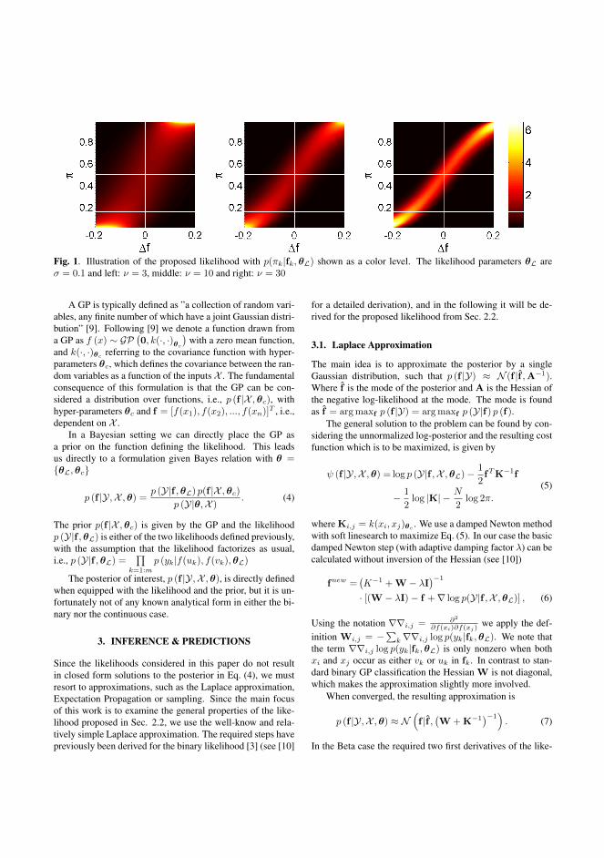
Fig. 1. Illustration of the proposed likelihood with p(πk|fk,θL) shown as a color level. The likelihood parameters θL areσ = 0.1 and left: ν = 3, middle: ν = 10 and right: ν = 30
A GP is typically defined as ”a collection of random vari-ables, any finite number of which have a joint Gaussian distri-bution” [9]. Following [9] we denote a function drawn froma GP as f (x) ∼ GP
(0, k(·, ·)θc
)with a zero mean function,
and k(·, ·)θc referring to the covariance function with hyper-parameters θc, which defines the covariance between the ran-dom variables as a function of the inputs X . The fundamentalconsequence of this formulation is that the GP can be con-sidered a distribution over functions, i.e., p (f |X ,θc), withhyper-parameters θc and f = [f(x1), f(x2), ..., f(xn)]T , i.e.,dependent on X .
In a Bayesian setting we can directly place the GP asa prior on the function defining the likelihood. This leadsus directly to a formulation given Bayes relation with θ ={θL,θc}
p (f |Y,X ,θ) =p (Y|f ,θL) p(f |X ,θc)
p (Y|θ,X ). (4)
The prior p(f |X ,θc) is given by the GP and the likelihoodp (Y|f ,θL) is either of the two likelihoods defined previously,with the assumption that the likelihood factorizes as usual,i.e., p (Y|f ,θL) =
∏k=1:m
p (yk|f(uk), f(vk),θL)
The posterior of interest, p (f |Y,X ,θ), is directly definedwhen equipped with the likelihood and the prior, but it is un-fortunately not of any known analytical form in either the bi-nary nor the continuous case.
3. INFERENCE & PREDICTIONS
Since the likelihoods considered in this paper do not resultin closed form solutions to the posterior in Eq. (4), we mustresort to approximations, such as the Laplace approximation,Expectation Propagation or sampling. Since the main focusof this work is to examine the general properties of the like-lihood proposed in Sec. 2.2, we use the well-know and rela-tively simple Laplace approximation. The required steps havepreviously been derived for the binary likelihood [3] (see [10]
for a detailed derivation), and in the following it will be de-rived for the proposed likelihood from Sec. 2.2.
3.1. Laplace Approximation
The main idea is to approximate the posterior by a singleGaussian distribution, such that p (f |Y) ≈ N (f |f ,A−1).Where f is the mode of the posterior and A is the Hessian ofthe negative log-likelihood at the mode. The mode is foundas f = arg maxf p (f |Y) = arg maxf p (Y|f) p (f).
The general solution to the problem can be found by con-sidering the unnormalized log-posterior and the resulting costfunction which is to be maximized, is given by
ψ (f |Y,X ,θ) = log p (Y|f ,X ,θL)− 1
2fTK−1f
− 1
2log |K| − N
2log 2π.
(5)
where Ki,j = k(xi, xj)θc . We use a damped Newton methodwith soft linesearch to maximize Eq. (5). In our case the basicdamped Newton step (with adaptive damping factor λ) can becalculated without inversion of the Hessian (see [10])
fnew =(K−1 + W − λI
)−1
· [(W − λI)− f +∇ log p(Y|f ,X ,θL)] , (6)
Using the notation ∇∇i,j = ∂2
∂f(xi)∂f(xj)we apply the def-
inition Wi,j = −∑k∇∇i,j log p(yk|fk,θL). We note thatthe term ∇∇i,j log p(yk|fk,θL) is only nonzero when bothxi and xj occur as either vk or uk in fk. In contrast to stan-dard binary GP classification the Hessian W is not diagonal,which makes the approximation slightly more involved.
When converged, the resulting approximation is
p (f |Y,X ,θ) ≈ N(f |f ,
(W + K−1
)−1). (7)
In the Beta case the required two first derivatives of the like-

lihood are given by:
∇i log p(πk | fk,θL) = I(xi) · ν · N (fk)
· [log(πk)− log(1− πk)− ψ(α) + ψ(β)] and (8)
∇∇i,j log p(πk | fk,θL) = −I(xi)I(xj) · ν2 · N (fk) ,
·[N (fk) ·
(ψ(1)(α) + ψ(1)(β)
)+f(vk)− f(uk)
2νσ2
· (log(πk)− log(1− πk)− ψ(α) + ψ(β))] , (9)
where we for convenience write α and β without the de-pendency on fk Eq. (2). ψ(z) and ψ(1)(z) are the digammafunction of zero’th and first order, respectively, N (fk) =
N(f(vk)−f(uk)√
2σ
∣∣∣ 0, 1)
and I(z) is an indicator function de-fined by
I(z) =
1 if z = uk−1 if z = vk
0 otherwise.(10)
We refer to [10] for a full derivation and for the requiredderivatives for the binary case as first described in [3].
3.2. Hyper-parameter Estimation
So far we have simply considered the hyper-parameters θ ={θL,θc} variables on which we can condition the primaryposterior, and not worried about their values or distributions.In the following, we consider the hyper-parameters randomvariables on which we place a prior and the full posteriorwould be p (f ,θ|Y). However, since the focus in this workis p (f |Y,X ,θ) we only use the prior on θ to make pointestimates of the hyper-parameters in terms of maximum-a-posteriori (MAP) estimates.
We obtain the MAP estimates by iterating between theLaplace approximation with fixed hyper-parameters, i.e.finding p (f |Y,X ,θMAP), followed by a maximization stepin which θMAP = arg maxθp (θ|Y,X , f).
We first consider the standard evidence approach whichseeks to optimize the marginal likelihood given by
p(Y|θ,X ) =
∫p(Y|f ,θL)p(f |X ,θc)df
= p(θ|Y,X )p(Y|X )/p(θ|X ). (11)
Our interest is in the posterior term, p(θ|Y,X ), so consid-ering Eq. (11) in terms of the log-posterior of θ we obtainlog p (θ|Y,X ) = log p (θ|X )+log p (Y|θ,X )−log p (Y|X ),where p (θ|X ) is the prior and typical considered indepen-dent of X . The evidence term, log p(Y|θ,X ), is analyticalintractable in both likelihood cases, but we can approximateit using the existing Laplace approximation to obtain [10]log p (Y|θ) ≈ log p(Y|f ,θL)− 1
2 fTK−1f− 1
2 log |I + KW |.Now θMAP is found by maximizing log p (θ|Y,X ) with re-spect to θ and noting that p(Y|X ) is independent of θ. Weperform the optimization using a BFGS gradient method. Therequired derivatives and details are provided in [10].
The choice of particular priors is left for the simulationsin Sec. 4, however, if p(θ) is the Uniform distribution, weobtain the traditional evidence optimization [9] as expected.It is noted that the complexity of the posterior inference is ofthe same order as standard GP regression described in [9].
3.3. Prediction
The main task is to estimate the latent function, f , with theend goal to do predictions of the observable variable y for apair of test inputs r ∈ Xt and s ∈ Xt. In this paper, we areespecially interested in the discrete decision, i.e., whether r �s or s � r. This can be obtained from both likelihood models,thus allowing for direct comparison of the two formulationsin terms of predictive performance.
We first consider the predictive distribution of f whichis required in both cases, and for notational convenience weomit the conditioning on X and Xt. Given the GP, we canwrite the joint prior distribution between f ∼ p (f |Y,θMAP)
and the test variables ft = [f (r) , f (s)]T as
[f
ft
]= N
([0
0
],
[K ktkTt Kt
]), (12)
where kt is a matrix with elements k2,i = k(s, xi)θMAPc
andk1,i = k(r, xi)θMAP
cwith xi being a training input. The con-
ditional p (ft|f) is obviously Gaussian as well and can be ob-tained directly from Eq. (12). The predictive distribution isgiven as p (ft|Y,θMAP) =
∫p (ft|f) p (f |Y,θMAP) df . With the
posterior approximated with the Gaussian from the Laplaceapproximation then p (ft|Y,θMAP) will be Gaussian too and isgiven as N (ft|µ∗,K∗) with µ∗ = [µ∗r , µ
∗s]T = ktK
−1f and
K∗ =
[K∗rr K∗rsK∗sr K∗ss
]= Kt − kTt (I + WK)kt,
where f and W are obtained from Eq. (7). With the predictivedistribution for ft, the final prediction of the observed variableis available from
p (yt|Y,θMAP) =
∫p (yt|ft,θMAP
L ) p (ft|Y,θMAP) dft (13)
If the likelihood is an odd function, as in both our cases, thebinary preference decision between r and s can be made di-rectly from p (ft|Y). In contrast, evaluation of the integral inEq. (13) is required for, e.g., soft decisions, reject options andsequential designs.
3.3.1. Binary Likelihood
If p(ft|Y,θMAP) is Gaussian and we consider the Probit like-
lihood, the integral in Eq. (13) can be evaluated in closed formas a modified Probit function given by [3]
P (r � s|Y) = Φ ((µ∗r − µ∗s) /σ∗) (14)
with (σ∗)2 = 2σ2 + K∗rr + K∗ss −K∗rs −K∗sr

−5 0 5−3
−2
−1
0
x
f(x)
Fig. 2. The Griewangk function used to evaluate the predic-tive performance. Crosses indicate discrete samples. The cen-ter peak is slightly higher than the two others.
3.3.2. Continuous Likelihood
In the continuous case the observed variable, π, does not di-rectly define the discrete observation which is the main focusof this work. However, a binary preference can be derivedfrom the continuous likelihood via the predictive distributionover π. With the suggested likelihood and mean function inSec. 2.2 the probability of the binary choice is obtained asP (r � s|Y,θL) =
∫ π=1/2
π=0p (πt|Y,θL) dπt, thus
P (r � s|Y,θMAP) =∫p(ft|Y,θMAP)Betacdf
(1
2
∣∣∣α(ft), β(ft)
)dft (15)
In the ideal case of a noise-free user, i.e., ν → ∞, the Betadistribution reduces to a point mass at the mean defined by theProbit function. Hence, in the limit of a completely consis-tent user, the predictions from Eq. (15) reduces to a classicalchoice model with predictions that follows Eq. (14).
4. EXPERIMENTAL RESULTS AND DISCUSSION
To study the performance of the models in a controlled set-ting, we use a synthetic dataset generated from the deter-ministic Griewangk function depicted in Fig. 2. We use thepredictive performance of the binary decision to compare thelearning rates of the binary response (BR) model as the base-line and the continuous bounded response (CBR) model. Ineach comparison, the two inputs are drawn randomly among101 input points sampled uniformly from x = [−8; 8].
The training points πk are drawn from a Beta distributionwith the parameterization from Sec. 2.2 with the Probit linkfunction in Eq. (4), σ = 1, and the Griewangk function val-ues as the two inputs. The noise level on the training data isdefined by the parameter νD corresponding to ν in the CBRmodel. The binary decision dk is determined by whether πkis smaller or larger than 0.5. For evaluation, we generate anindependent binary test set located equidistantly in betweenthe training points. Initial experiments showed that in or-der to get a robust predictive model for all noise level, it isimportant to learn the ν parameter in the CBR model. The
Simulation Data Noise θL θc
νD σ ν σf lBR NoiseFree No Noise δ1 δideal δideal
BR {3, 10, 30} δ1 U1 U1
CBR NoiseFree No Noise δ1 δ→∞ δideal δideal
CBR Ideal {3, 10, 30} δ1 δ{3,10,30} δideal δideal
CBR {3, 10, 30} δ1 G(1, η){3,10,30} U1 U1
Table 1. Simulation conditions. δx is a point-mass, thus theparameter is constantly equal to x. The δideal value is learnedas m → ∞. Ux is an uniform prior over ]0;∞[ with theparameter initialized to x. G(1, η)x is a Gamma prior withinverse scale parameter η = 0.05 and initialization x.
initial experiments also indicated that it is vital not to under-estimate the noise, while an overestimation is not as crucialand provides overall good predictive performance. This sug-gests a prior with a monotonic increasing likelihood towardsthe highest noise level. A natural choice is a Gamma(1,η)prior with inverse scale parameter η.
The considered models, priors and parameters are listed inTable 1 where the covariance parameters, θc, are applied in aGP prior with a covariance function defined by the squaredexponential kernel kSE(x, x′) = σ2
f exp(−l−2‖x− x′‖2).When a specific prior is not a point-mass/constant indicatedby δx in Table 1, the hyper-parameters are estimated (MAP)either for each training set size (realistic scenario) or for m =500 (ideal scenario). The latter is indicated by δideal.
The learning curves from Fig. 3 show that under idealconditions with nearly noise-free observations and a correctnoise setting (Fig. 3, right plot) the CBR model outperformsthe BR models as expected, since a continuous response willessentially provide more information from each experimentunder ideal conditions than a binary response will. Also, inboth high and moderate noise conditions (Fig. 3, left and mid-dle plot) the CBR model with a correct noise setting (CBRIdeal) outperforms the corresponding BR model significantlyin terms of learning rates and actually shows similar learn-ing rates as the BR model under noise-free conditions. Fi-nally and most importantly, the learning rates are only slightlylower when ν has been inferred from data via the MAP pro-cedure (with different initializations) than when it is specifiedcorrectly, which suggests that the parameter inference frame-work with independent priors is robust in real-life-scenarioswithout ideal model and noise conditions.
We have focused on a controlled example to highlightproperties of the model and inference, leaving a real-worldvalidation for future work. Future work also includes theextension of the mean function, Eq. (4), using a mixture ofProbit functions to account for different user behavior suchas centering and contraction bias. For a real-world setting, anatural extension is a suitable active learning criteria, such asthe expected value of information framework applied recentlyin e.g. [5] for the BR model.

Fig. 3. Mean error test rates (MER) as a function of the number of experiments over 100 different realizations of the trainingset generated with different νD. In the red and top green area MER are worse and better, respectively, than those obtained withthe BR model on the noisy data. In the lower green area MER are also better than those obtained by the BR NoiseFree, andfinally, the grey area corresponds to unrealistic MER better than those obtained with a CBR NoiseFree model with ν → ∞evaluated with ν = 103 on a noise-free data set. The six rows of markers indicate if the MER of the corresponding CBRmodel are significantly different from those resulting from the BR (squares) and from the BR NoiseFree (circles). If solid, thezero-hypothesis of the two means being equal is rejected at the 5% level using a paired t-test.
5. CONCLUSION AND PERSPECTIVES
We have proposed a new model for preference learning withGaussian Process priors with the main purpose to increasethe learning rate compared to the standard binary model ap-plied in [3]. We have outlined a robust and flexible inferenceframework for the new model based on suitable priors andthe Laplace approximation. Simulations were used to presentproperties and performance, which showed a significant infor-mation increase from each experiment under ideal conditionsas expected but more importantly also under adverse condi-tions. The performance is especially increased in a certainwindow of opportunity.
Acknowledgement: This work was supported in part by the IST Pro-gramme of the European Community, under the PASCAL2 Networkof Excellence, IST-2007-216886. This publication only reflects theauthors’ views.
6. REFERENCES
[1] G. R. Lockhead, “Absolute Judgments Are Relative: AReinterpretation of Some Psychophysical Ideas.,” Re-view of General Psychology, vol. 8, no. 4, pp. 265–272,2004.
[2] L. L. Thurstone, “A law of comparative judgement.,”Psychological Review, vol. 34, 1927.
[3] W. Chu and Z. Ghahramani, “Preference learning withGaussian Processes,” ICML 2005 - Proceedings of the
22nd International Conference on Machine Learning,pp. 137–144, 2005.
[4] P. Groot, T. Heskes, T. Dijkstra, and J. Kates, “Pre-dicting preference judgments of individual normal andhearing-impaired listeners with Gaussian Processes,”IEEE Transactions on Audio, Sound, and LanguageProcessing, 2010.
[5] E. Bonilla, S. Guo, and S. Sanner, “Gaussian Pro-cess preference elicitation,” in Advances in Neural In-formation Processing Systems 23, J. Lafferty, C. K. I.Williams, J. Shawe-Taylor, R.S. Zemel, and A. Culotta,Eds., pp. 262–270. 2010.
[6] W. Chu and Z. Ghahramani, “Extensions of GaussianProcesses for ranking: semi-supervised and active learn-ing,” in Workshop Learning to Rank at Advances in Neu-ral Information Processing Systems 18, 2005.
[7] R. D. Bock and J. V. Jones, “The measurement and pre-diction of judgment and choice.,” 1968.
[8] S. Ferrari and F. Cribari-Neto, “Beta Regression forModelling Rates and Proportions,” Journal of AppliedStatistics, vol. 31, no. 7, pp. 799–815, Aug. 2004.
[9] C. E. Rasmussen and C. K. I. Williams, Gaussian Pro-cesses for Machine Learning, MIT Press, 2006.
[10] Bjørn Sand Jensen and Jens Brehm Nielsen, Pair-wise Judgements and Absolute Ratings with GaussianProcess Priors, Technical Report, DTU Informatics,September 2011.

Appendix D
A Predictive Model of MusicPreference using Pairwise
Comparisons
Bjørn Sand Jensen, Javier Saez Gallego and Jan Larsen. A Predictive modelof music preference using pairwise comparisons. International Conference onAcoustics, Speech, and Signal Processing (ICASSP) 2012. Published.

116 Appendix D

A PREDICTIVE MODEL OF MUSIC PREFERENCE USING PAIRWISE COMPARISONS
Bjørn Sand Jensen, Javier Saez Gallego & Jan Larsen∗
Technical University of Denmark, Department of Informatics andMathematical Modeling, Richard Petersens Plads B321
2800 Lyngby, Denmark
ABSTRACTMusic recommendation is an important aspect of many
streaming services and multi-media systems, however, it istypically based on so-called collaborative filtering methods.In this paper we consider the recommendation task from apersonal viewpoint and examine to which degree music pref-erence can be elicited and predicted using simple and robustqueries such as pairwise comparisons. We propose to model- and in turn predict - the pairwise music preference usinga very flexible model based on Gaussian Process priors forwhich we describe the required inference. We further proposea specific covariance function and evaluate the predictive per-formance on a novel dataset. In a recommendation style set-ting we obtain a leave-one-out accuracy of 74% compared to50% with random predictions, showing potential for furtherrefinement and evaluation.
Index Terms— Music Preference, Kernel Methods,Gaussian Process Priors, Recommendation
1. INTRODUCTION
Methods for music recommendation has received a great dealof attention the last decade with most approaches typically be-ing classified as collaborative filtering (top-down) or content-based (bottom-up) methods, with hybrid methods (see e.g.[1]) comprising both. Such hybrid systems exploits both rat-ings and contents to make recommendations, but the focusis still on the recommendation itself and not the basic ques-tions of preference. Although from a fundamental point ofview it is also interesting how well human preference can beelicited and represented without relying on the help of oth-ers. This also includes the aim to answer basic questions suchas which properties of music determines the persons musicpreference. Obviously the potential power of collaborativefiltering should not be discarded, but exploited in a princi-pled manner in order to answer basic questions and hopefully
∗This work was supported in part by the IST Programme of theEuropean Community, under the PASCAL2 Network of Excellence,IST-2007-216886. This publication only reflects the authors’ views.∗∗ This work was supported in part by the Danish Council for Strategic Re-search of the Danish Agency for Science Technology and Innovation underthe CoSound project, case number 11-115328.
provide an even better predictive model of individual musicpreference.
Based on these observations we consider music prefer-ence in a personalized setting by applying a Gaussian Processregression model which takes into account both human rat-ings and audio features. In contrast to many audio rating sys-tems it is not based on absolute ratings of a single track, buton a pairwise comparisons between tracks, which is typicallyconsidered robust and have a low cognitive load (see e.g. [2]).
We furthermore propose to use a covariance function mo-tivated from a generative view of audio features with a po-tential multi-task part which lead to similar capabilities asstandard collaborative filtering, but with the added informa-tion level provided by subject features. Posterior inferencein the resulting non-parametric Bayesian regression model isperformed using a Laplace approximation of the otherwise in-tractable distribution. Any hyperparameters in the model canbe learned using an empirical Bayes approach.
We evaluate the resulting model by its predictive poweron a small scale, public available dataset [3] where 10 sub-jects evaluate 30 tracks in 3 genres. We report and discussa number of aspects of the performance such as the learningcurves as a function of the number of pairwise comparisonsand learning curves when leaving out a track as test set.
2. METHODS
In this work we focus on modeling preference elicited by pair-wise queries, i.e., given two inputs tracks u and v we ob-tain a response, y ∈ {−1, 1}, where y = −1 correspondsto a preference for u, and +1 corresponds to a preferencefor v. We consider n distinct input tracks xi ∈ X denotedX = {xi|i = 1, ..., n}, and a set of m responses on pairwisecomparisons between any two inputs in X , denoted by
Y = {(yk;uk, vk)|k = 1, ...,m} ,
where yk ∈ {−1, 1}. uk ∈ X and vk ∈ X are option one andtwo in the k’th pairwise comparison.
We consider yk as a stochastic variable and we can thenformulate the likelihood of observing a given response as cu-

mulative normal distribution.
p (yk|fk,θL) = Φ
(ykf (vk)− f (uk)√
2σ
), (1)
with fk = [f (uk) , f (vk)], Φ(x) defines a cumulative Gaus-sian (with zero mean and unity variance) and θL = {σ}. Thisis in turn the well known Probit classification model, wherethe argument is the difference between two latent variables(functional values) and not just a single latent variable. Thisin effect implies that the f(·) encodes an internal, but latentpreference function which can be elicited by pairwise com-parisons via the likelihood model in Eq.( 1). This idea wasalready considered by [4], but recently suggested in a Gaus-sian Process context by [5].
2.1. Gaussian Process Prior
The real question remains, namely how f is modelled. Wewill follow the principle suggested by [5] in which f is con-sidered an abstract function and we can in turn place a priordistribution over it. A natural prior is a Gaussian Process(GP) defined as ”a collection of random variables, any finitenumber of which have a (consistent) joint Gaussian distribu-tion” [6]. Following [6] we denote a function drawn from aGP as f (x) ∼ GP
(0, k(·, ·)θc
)with a zero mean function,
and k(·, ·)θcreferring to the covariance function with hyper-
parameters θc, which defines the covariance between the ran-dom variables as a function of the inputsX . The consequenceof this formulation is that the GP can be considered a distri-bution over functions, i.e., p (f |X ,θc), with hyper-parametersθc and f = [f(x1), f(x2), ..., f(xn)]T .
In a Bayesian setting we can directly place the GP asa prior on the function defining the likelihood. This leadsus directly to a formulation given Bayes relation with θ ={θL,θc}
p (f |Y,X ,θ) =p (Y|f ,θL) p(f |X ,θc)
p (Y|θ,X ). (2)
The prior p(f |X ,θc) is given by the GP and the likeli-hood p (Y|f ,θL) is the two likelihood defined previously,with the usual assumption that the likelihood factorizes, i.e.,p (Y|f ,θL) =
∏k=1:m
p (yk|f(uk), f(vk),θL)
The posterior of interest, p (f |Y,X ,θ), is defined whenequipped with the likelihood and the prior, but it is unfortu-nately not of any known analytical form, thus we rely on theLaplace approximation.
2.2. Inference & Hyperparameters
We apply the Laplace approximation and approximate theposterior by a multivariate Gaussian distribution, such thatp (f |Y) ≈ N (f |f ,A−1). Where f is the mode of the pos-terior and A is the Hessian of the negative log-likelihood atthe mode.
The mode is found as f = arg maxf p (Y|f) p (f). Wesolve the problem by considering the unnormalized log-posterior and the resulting cost function which is to be maxi-mized, is given by
ψ (f |Y,X ,θ) = log p (Y|f ,X ,θL)− 1
2fTK−1f
− 1
2log |K| − N
2log 2π.
(3)
where Ki,j = k(xi, xj)θc. We use a damped Newton method
with soft linesearch to maximize Eq. (3). In our case the basicdamped Newton step (with adaptive damping factor λ) can becalculated without inversion of the Hessian (see [7])
fnew =(K−1 + W − λI
)−1
· [(W − λI)− f +∇ log p(Y|f ,X ,θL)] , (4)
Using the notation ∇∇i,j = ∂2
∂f(xi)∂f(xj)we apply the def-
inition Wi,j = −∑k∇∇i,j log p(yk|fk,θL). We note thatthe term∇∇i,j log p(yk|fk,θL) is only nonzero when both xiand xj occur as either vk or uk in fk. In contrast to standardbinary GP classification, the negative Hessian, W is not diag-onal, which makes the approximation slightly more involved.When converged, the resulting approximation is
p (f |Y,X ,θ) ≈ N(f |f ,
(W + K−1
)−1). (5)
We refer to [7] for a full derivation and for the required deriva-tives as first outlined in [5]. Parameters in the likelihood andcovariance function, collected in θ, are found by evidence op-timization using a standard BFGS method.
2.3. Predictions & Evaluations
Given the model, in essence defined by f , we wish to makepredictions of the observed variable y for a pair of test in-puts r ∈ Xt and s ∈ Xt. We are especially interested inthe discrete decision, i.e., whether r is preferred over s de-noted by r � s, or vice versa. Omitting the conditioning onX and Xt, we can write the joint prior distribution betweenf ∼ p (f |Y,θ) and the test variables ft = [f (r) , f (s)]
T as[f
ft
]= N
([0
0
],
[K kt
kTt Kt
]), (6)
where kt is a matrix with elements k2,i = k(s, xi)θc andk1,i = k(r, xi)θc with xi being a training input. The con-ditional p (ft|f) is obviously Gaussian as well and can beobtained directly from Eq. (6). The predictive distributionis given as p (ft|Y,θ) =
∫p (ft|f) p (f |Y,θ) df . With the
posterior approximated with the Gaussian from the Laplaceapproximation, then p (ft|Y,θ) will be Gaussian too and isgiven as N (ft|µ∗,K∗) with µ∗ = [µ∗r , µ
∗s]T = ktK
−1f and
K∗ =
[K∗rr K∗rsK∗sr K∗ss
]= Kt − kT
t (I + WK)kt,
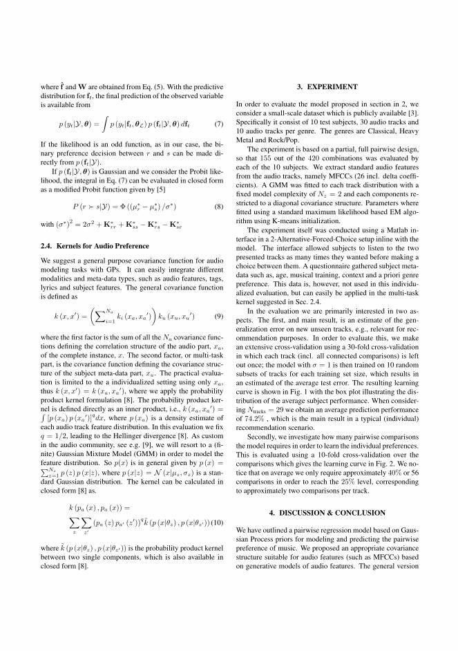
where f and W are obtained from Eq. (5). With the predictivedistribution for ft, the final prediction of the observed variableis available from
p (yt|Y,θ) =
∫p (yt|ft,θL) p (ft|Y,θ) dft (7)
If the likelihood is an odd function, as in our case, the bi-nary preference decision between r and s can be made di-rectly from p (ft|Y).
If p (ft|Y,θ) is Gaussian and we consider the Probit like-lihood, the integral in Eq. (7) can be evaluated in closed formas a modified Probit function given by [5]
P (r � s|Y) = Φ ((µ∗r − µ∗s) /σ∗) (8)
with (σ∗)2 = 2σ2 + K∗rr + K∗ss −K∗rs −K∗sr
2.4. Kernels for Audio Preference
We suggest a general purpose covariance function for audiomodeling tasks with GPs. It can easily integrate differentmodalities and meta-data types, such as audio features, tags,lyrics and subject features. The general covariance functionis defined as
k (x, x′) =
(∑Na
i=1ki (xa, xa
′)
)ku (xu, xu
′) (9)
where the first factor is the sum of all theNa covariance func-tions defining the correlation structure of the audio part, xa,of the complete instance, x. The second factor, or multi-taskpart, is the covariance function defining the covariance struc-ture of the subject meta-data part, xu. The practical evalua-tion is limited to the a individualized setting using only xa,thus k (x, x′) = k (xa, xa
′), where we apply the probabilityproduct kernel formulation [8]. The probability product ker-nel is defined directly as an inner product, i.e., k (xa, xa
′) =∫[p (xa) p (xa
′)]qdx, where p (xa) is a density estimate ofeach audio track feature distribution. In this evaluation we fixq = 1/2, leading to the Hellinger divergence [8]. As customin the audio community, see e.g. [9], we will resort to a (fi-nite) Gaussian Mixture Model (GMM) in order to model thefeature distribution. So p(x) is in general given by p (x) =∑Nz
z=1 p (z) p (x|z), where p (x|z) = N (x|µz, σz) is a stan-dard Gaussian distribution. The kernel can be calculated inclosed form [8] as.
k (pa (x) , pa (x)) =∑
z
∑
z′
(pa (z) pa′ (z′))qk (p (x|θz) , p (x|θz′)) (10)
where k (p (x|θz) , p (x|θz′)) is the probability product kernelbetween two single components, which is also available inclosed form [8].
3. EXPERIMENT
In order to evaluate the model proposed in section in 2, weconsider a small-scale dataset which is publicly available [3].Specifically it consist of 10 test subjects, 30 audio tracks and10 audio tracks per genre. The genres are Classical, HeavyMetal and Rock/Pop.
The experiment is based on a partial, full pairwise design,so that 155 out of the 420 combinations was evaluated byeach of the 10 subjects. We extract standard audio featuresfrom the audio tracks, namely MFCCs (26 incl. delta coeffi-cients). A GMM was fitted to each track distribution with afixed model complexity of Nz = 2 and each components re-stricted to a diagonal covariance structure. Parameters wherefitted using a standard maximum likelihood based EM algo-rithm using K-means initialization.
The experiment itself was conducted using a Matlab in-terface in a 2-Alternative-Forced-Choice setup inline with themodel. The interface allowed subjects to listen to the twopresented tracks as many times they wanted before making achoice between them. A questionnaire gathered subject meta-data such as, age, musical training, context and a priori genrepreference. This data is, however, not used in this individu-alized evaluation, but can easily be applied in the multi-taskkernel suggested in Sec. 2.4.
In the evaluation we are primarily interested in two as-pects. The first, and main result, is an estimate of the gen-eralization error on new unseen tracks, e.g., relevant for rec-ommendation purposes. In order to evaluate this, we makean extensive cross-validation using a 30-fold cross-validationin which each track (incl. all connected comparisons) is leftout once; the model with σ = 1 is then trained on 10 randomsubsets of tracks for each training set size, which results inan estimated of the average test error. The resulting learningcurve is shown in Fig. 1 with the box plot illustrating the dis-tribution of the average subject performance. When consider-ingNtracks = 29 we obtain an average prediction performanceof 74.2% , which is the main result in a typical (individual)recommendation scenario.
Secondly, we investigate how many pairwise comparisonsthe model requires in order to learn the individual preferences.This is evaluated using a 10-fold cross-validation over thecomparisons which gives the learning curve in Fig. 2. We no-tice that on average we only require approximately 40% or 56comparisons in order to reach the 25% level, correspondingto approximately two comparisons per track.
4. DISCUSSION & CONCLUSION
We have outlined a pairwise regression model based on Gaus-sian Process priors for modeling and predicting the pairwisepreference of music. We proposed an appropriate covariancestructure suitable for audio features (such as MFCCs) basedon generative models of audio features. The general version
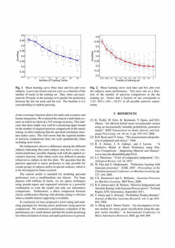
0.1
0.15
0.2
0.25
0.3
0.35
0.4
0.45
0.5
2 4 8 12 16 20 24 29Number of Training Tracks
Err
orR
ate
Fig. 1. Mean learning curve (blue line) and box plot oversubjects. Leave-one-(track)-out test error as a function of thenumber of tracks in the training set. Thus, there can maxi-mum be 29 tracks in the training set to predict the preferencebetween the left out track and the rest. The baseline is 0.5corresponding to random guessing.
of the covariance function allows for multi-task scenarios andfeature integration. We evaluated the setup in a individual sce-nario in which we showed a 74% average accuracy. This indi-cates that there might very well be a promising upper boundon the number of required pairwise comparisons in this musicsetting, in effect implying that the specified correlation struc-ture makes sense. This will ensure that the required numberof pairwise comparisons does not scale quadratically whenincluding more tracks.
We furthermore observe a difference among the differentsubjects indicating that some subjects may have a very con-sistent preference, possibly aligning well with the applied co-variance function, while others seem very difficult to predict(observed as outliers in the box plot). We speculate that thepairwise approach to music preference is only possible forcertain groups of subjects and/or in special contexts, which isto be investigated in future research.
The current model is intended for modeling personalpreferences over a small/medium size dataset. For largedatasets with millions of tracks, we see sparse techniquesusing pseudo-inputs and sequential selection as a powerfulcombination to scale the model and only use informativecomparisons. Furthermore, a direct comparison betweenclassic collaborative filtering with absolute ratings is obviouswhen a suitable dataset supporting is available.
In conclusion we have proposed a novel rating and mod-eling paradigm for eliciting music preference using pairwisecomparisons. We conducted a preliminary evaluation of theperformance on a small dataset and find the results promisingfor robust elicitation of music and audio preference in general.
0.1
0.15
0.2
0.25
0.3
0.35
0.4
0.45
0.5
0.01 0.05 0.1 0.2 0.3 0.4 0.5 0.6 0.7 0.8 0.9 1Fraction of training set
Err
orR
ate
Fig. 2. Mean learning curve (red line) and box plot overthe subjects mean performance. Test error rate as a func-tion of the number of pairwise comparisons in the thetraining set. Notice that a fraction of one corresponds to(155 · 90%) /420 ∼ 33.2% of all possible pairwise experi-ments.
5. REFERENCES
[1] K. Yoshii, M. Goto, K. Komatani, T. Ogata, and H.G.Okuno, “An efficient hybrid music recommender systemusing an incrementally trainable probabilistic generativemodel,” IEEE Transactions on Audio, Speech, and Lan-guage Processing, vol. 16, no. 2, pp. 435–447, 2008.
[2] R.D. Bock and J.V. Jones, “The measurement and predic-tion of judgment and choice,” 1968.
[3] B. S. Jensen, J. S. Gallego, and J. Larsen, “APredictive Model of Music Preference using Pair-wise Comparisons - Supporting Material and Dataset,”www.imm.dtu.dk/pubdb/p.php?6143.
[4] L L Thurstone, “A law of comparative judgement,” Psy-chological Review, vol. 34, 1927.
[5] W. Chu and Z. Ghahramani, “Preference learning withGaussian processes,” ICML 2005 - Proceedings of the22nd International Conference on Machine Learning, pp.137–144, 2005.
[6] C.E. Rasmussen and C. Williams, Gaussian Processesfor Machine Learning, MIT Press, 2006.
[7] B. S. Jensen and J. B. Nielsen, “Pairwise Judgements andAbsolute Ratings with Gaussian Process priors,” TechinalReport, DTU Informatics, September 2011.
[8] T. Jebara and A. Howard, “Probability Product Kernels,”Journal of Machine Learning Research, vol. 5, pp. 819–844, 2004.
[9] A. Meng and J. Shawe-Taylor, “An investigation of fea-ture models for music genre classification using the sup-port vector classifier,” in International Conference onMusic Information Retrieval, 2005, pp. 604–609.
Appendix E
Towards Predicting ExpressedEmotion in Music from
Pairwise Comparisons

122 Appendix E

Towards Predicting Expressed Emotion in Music from Pairwise Comparisons
Jens Madsen, Bjørn Sand Jensen, Jan Larsen and Jens Brehm NielsenTechnical University of Denmark,
Department of Informatics and Mathematical Modeling,Asmussens Alle B321
2800 Kongens Lyngby, Denmark{jenma,bjje,jl,jenb}@imm.dtu.dk
ABSTRACT
We introduce five regression models for the modeling ofexpressed emotion in music using data obtained in a twoalternative forced choice listening experiment. The pre-dictive performance of the proposed models is comparedusing learning curves, showing that all models converge toproduce a similar classification error. The predictive rank-ing of the models is compared using Kendall’s τ rank cor-relation coefficient which shows a difference despite simi-lar classification error. The variation in predictions acrosssubjects and the difference in ranking is investigated vi-sually in the arousal-valence space and quantified usingKendall’s τ .
1. INTRODUCTION
The possibility to recommend music which express a cer-tain mood or emotion has recently gathered increasing at-tention within the Music Information Retrieval (MIR) com-munity.
Typically the recommendation is approached using com-putational methods, where music is represented using struc-tural features, such as features based on the audio signalthat mimic some functions of the human auditory percep-tive system, and possibly features representing even higheraspects of the human cognitive system. Research is on-going in finding what features can capture aspects in themusic that express or induce emotions see e.g. [1]. Fur-thermore, it is well known that there is a clear connectionbetween lyrics and the audio in music [2] and lyrical fea-tures have equally been shown to produce good results [3].Even contextual information about music can be utilizedfor the prediction of emotions in music using social mediacontents [4].
Despite the many meaningful audio features and repre-sentations, most computational models are supervised andrely on human participants to rate a given excerpt. Theseratings are mapped using supervised machine learning ap-proaches under the assumption that the model is the samefor all musical excerpts, thus the projection into feature
Copyright: c©2012 Jens Madsen, Bjørn Sand Jensen, Jan Larsen and Jens
Brehm Nielsen . This is an open-access article distributed under the terms of the
Creative Commons Attribution 3.0 Unported License, which permits unrestricted
use, distribution, and reproduction in any medium, provided the original author
and source are credited.
space is based on the same model for all excerpts and typ-ically also for all participants. Instead of obtaining deci-sions from subjects, unsupervised methods have recentlybeen proposed which can be used to find emotional cate-gories of excerpts [5]. The decision of what machine learn-ing method to apply is tightly connected to the chosen mu-sic representation and what emotional representation [6],and in this work we consider the supervised setting.
Expressed emotions in music are typically rated based onsimple self-reporting listening experiments [7] where thescales are adapted to quantify for example the categori-cal [8] or dimensional [9] models of emotion. Althoughthere is not one simple way of doing this and numerousdifferent approaches have been made to obtain these rat-ings e.g. using majority ruling, averaging across ratings,etc. in both domains even using combinations of the emo-tional models [10]. Another aspect to take into accountwhen creating computational models of emotion, is that itis well known that emotional expression in music changesover time which could further refine a recommendationmethod. Two main direction has been followed in obtain-ing time depend ratings. The first is based on post rat-ings of excerpts in the 15-30 s range under the assumptionthat within this frame the emotional expression is approx-imately constant. Machine learning techniques can thenbe used to create models making predictions on a smallertime scale using the post ratings of larger excerpts [12].The other direction is to continuously measure expressedemotions in music directly in e.g the arousal and valencespace (AV space) [11] and subsequently model this.
In [13] we proposed an alternative way of quantifying theexpressed emotion in music on the dimensions of valenceand arousal by introducing a two alternative force choice(2AFC) post rating experimental paradigm. Given the rela-tive nature of pairwise comparisons they eliminate the needfor an absolute reference anchor, which can be a problemin direct scaling experiments. Furthermore the relative na-ture persist the relation to previous excerpts reducing mem-ory effects. We use 15 s excerpts to minimize any changein expressed emotion over time, and large enough not tocause mental strain on subjects. We proposed a proba-bilistic Gaussian process framework for mapping the ex-tracted audio features into latent subspaces that is learnedby the comparisons made by participants of musical ex-cerpts evaluated on the dimensions of valence and arousal.The underlying assumption is that given the features, the

projection made by the model mimic the cognitive decisionmaking by participants in making the pairwise compari-son. We investigated how many comparisons are neededper excerpt to reach acceptable level of performance byobtaining all possible unique comparisons for 20 excerptsand furthermore to investigate the individual subjective dif-ferences. In [14] they proposed a greedy algorithmic ap-proach converting pairwise comparisons into a ranking ofexcerpts and modeling this using a RBF-ListNet algorithm.They focused on the case of few comparisons for many ex-cerpts, using comparisons from multiple participants ag-gregating to one large dataset, neglecting the individualdifferences between subjects. On the other hand, our re-sults showed a great difference between participants whichthe framework and approach accounts for along with noiseon the pairwise judgments.
These individual differences are further investigated inthis paper using the well known arousal and valance scoresin a 2D space. Furthermore, we introduce five models forthe modeling of the pairwise comparisons, where an ex-tension to the existing framework is made using linear andsquared exponential kernels. Moreover, we compare theGaussian process model to three versions of a General-ized Linear Model (GLM) namely the standard version andtwo regularized versions using L1 and L2 norms. Learn-ing curves are computed as a function of the misclassifi-cation error and the number of (randomly chosen) pair-wise comparisons in order to elucidate the difference be-tween the five models. The differences between modelsand the resulting ranking of excerpts is further illustratedusing Kendall’s τ rank correlation learning curves.
2. EXPERIMENT & DATA
2.1 Experiment
A listening experiment was conducted to obtain pairwisecomparisons of expressed emotion in music using a 2AFCexperimental paradigm. 20 different 15 second excerptswere chosen from the USPOP2002 1 dataset, so that, 5 ex-cerpts were chosen to be in each quadrant of the AV space.The selection was performed by a linear regression modeldeveloped in previous work. A subjective evaluation wasperformed to verify that the emotional expression of eachexcerpt was as constant as possible.
A sound booth provided neutral surroundings for the ex-periment and the excerpts were played back using head-phones to the 8 participants (2 female, 6 male). Writ-ten and verbal instructions were given prior to each ses-sion to ensure that subjects understood the purpose of theexperiment and to ensure that each subject were familiarwith the two emotional dimensions (valence and arousal).Each participant compared all 190 possible unique com-binations. For the arousal dimension, participants wereasked the question Which sound clip was the most excited,active, awake? For the valence dimension the question wasWhich sound clip was the most positive, glad, happy?. Thetwo dimensions was rated individually and the presentation
1 http://labrosa.ee.columbia.edu/projects/musicsim/uspop2002.html
No. Song name1 311 - T and p combo2 A-Ha - Living a boys adventure3 Abba - Thats me4 Acdc - What do you do for money honey5 Aaliyah - The one i gave my heart to6 Aerosmith - Mother popcorn7 Alanis Morissette - These r the thoughts8 Alice Cooper - Im your gun9 Alice in Chains - Killer is me
10 Aretha Franklin - A change11 Moby - Everloving12 Rammstein - Feuer frei13 Santana - Maria caracoles14 Stevie Wonder - Another star15 Tool - Hooker with a pen..16 Toto - We made it17 Tricky - Your name18 U2 - Babyface19 UB40 - Version girl20 ZZ top - Hot blue and righteous
Table 1. List of songs/excerpts.
of the 190 paired excepts was randomized. The details ofthe experiment is available in [15].
2.2 Audio Representation & Features
In order to represent the 15 second excerpts in later math-ematical models, each excerpt is represented by standardaudio features, namely Mel-frequency cepstral coefficients(MFCC) (30 dimensional), that describes the log trans-formed short-term power spectrum of the musical signal.Furthermore a total of 9 features are included namely spectral-flux, roll-off, slope and variation and 5 features describingthe temporal music signal including zero crossing rate andstatistical shape descriptors.
These features are extracted using the YAAFE toolbox 1
for 512 sample frames with 50% overlap, thus for each ex-cerpt we obtain a 39x1292 feature matrix X. We create avector representation by first standardizing the features andthen estimating the mean, µ(·) and the variance of the ma-trix var(·) over the frames and then applying the follow-ing vectorization, x = [µ (X) , var (X)]. This (row) vectorrepresentation can directly be used in standard modelingtools and serves as a common ground for comparisons.
3. MODELS FOR PAIRWISE COMPARISONS
The pairwise observations presented in Section 2 poses aspecial challenge since each output now depends on twoinputs and standard regression and classification tools donot immediately apply since they are typically formulatedin a one to one relationship between inputs and outputs.The modeling aspect will thus necessarily play an integralpart of this section, and we will initially outline the generalframework.
1 http://yaafe.sourceforge.net/
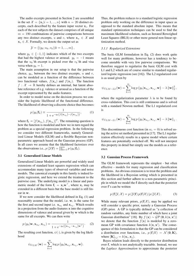
The audio excerpts presented in Section 2 are assembledin the set X = {xi|i = 1, ..., n} with n = 20 distinct ex-cerpts, each described by the feature input vector xi. Foreach of the test subjects the dataset comprises of all uniquem = 190 combinations of pairwise comparisons betweenany two distinct excerpts, u and v, where xu ∈ X andxv ∈ X . Formally, we denote the output set as
Y = {(yk;uk, vk)|k = 1, ...,m} ,where yk ∈ {−1, 1} indicates which of the two excerptsthat had the highest valence or arousal. yk = −1 meansthat the uk’th excerpt is picked over the vk’th and visaversa when yk = 1.
The main assumption in our setup is that the pairwisechoice, yk, between the two distinct excerpts, u and v,can be modeled as a function of the difference betweentwo functional values, f(xu) and f(xv). The functionf : X → R hereby defines an internal, but latent abso-lute reference of e.g. valence or arousal as a function of theexcerpt represented by the audio features.
In order to model noise on the decision process we con-sider the logistic likelihood of the functional difference.The likelihood of observing a discrete choice thus becomes:
p (yk|fk) ≡ 1
1 + e−yk(f(xuk)−f(xvk)), (1)
where fk = [f(xuk), f(xvk)]T . The remaining question is
how the function is modeled and how we in turn regard theproblem as a special regression problem. In the followingwe consider two different frameworks, namely General-ized Linear Models (GLM) and a flexible Bayesian non-parametric approach based on the Gaussian process (GP).In all cases we assume that the likelihood factorizes overthe observations i.e., p (Y|f) =
∏mk=1 p (yk|fk).
3.1 Generalized Linear Models
Generalized Linear Models are powerful and widely usedextensions of standard least squares regression which canaccommodate many types of observed variables and noisemodels. The canonical example in this family is indeed lo-gistic regression, and here we extend the treatment to thepairwise case. The underlying model is a linear and para-metric model of the form fi = xiw
>, where xi may beextended in a different basis but the base model is still lin-ear in w.
If we now consider the likelihood defined in Eq. (1) andreasonably assume that the model, i.e. w, is the same forthe first and second input i.e. xuk
and xvk . Which resultsin a projection from the audio features x into the cognitivedimensions of valence and arousal given by w which is thesame for all excerpts. We can then write
p (yk|w,xuk,xvk) =
1
1 + e−yk((xuk−xvk)w>)
. (2)
The resulting cost function, ψ(·), is given by the log likeli-hood
ψGLM (w) =
m∑
k=1
log p(yk|xuk
,xvk,w).
Thus, the problem reduces to a standard logistic regressionproblem only working on the difference in input space asopposed to the standard absolute input. This means thatstandard optimization techniques can be used to find themaximum likelihood solution, such as Iterated ReweighedLeast Squares (IRLS) or other more general non-linear op-timization method.
3.1.1 Regularized Extensions
The basic GLM formulation in Eq. (2) does work quitewell for many problems, however has a tendency to be-come unstable with very few pairwise comparisons. Wetherefore suggest to regularize the basic GLM cost withL1 and L2 which are of course similar to standard regular-ized logistic regression (see [16]). The L2 regularized costis as usual given by
ψGLM−L2 (w) =m∑
k=1
log p(yk|xuk
,xvk,w)− λ ‖w‖22 ,
where the regularization parameter λ is to be found bycross-validation. This cost is still continuous and is solvedwith a standard Newton method. The L1 regularized costis
ψGLM−L1 (w) =m∑
k=1
log p(yk|xuk
,xvk,w)− λ ‖w‖1 .
This discontinuous cost function (in wi = 0) is solved us-ing the active set method presented in [17]. The L1 regular-ization effectively results in a sparse model where certainfeatures are potentially switched off. We will not interpretthis property in detail but simply use the models as a refer-ence.
3.2 Gaussian Process Framework
The GLM framework represents the simplest - but ofteneffective - models for many regression and classificationproblems. An obvious extension is to treat the problem andthe likelihood in a Bayesian setting which is presented inthis section and further adhere to a non-parametric princi-ple in which we model the f directly such that the posteriorover f ’s can be written
p (f |Y,X ) = p (Y|f) p(f |X )/p (Y|X ) . (3)
While many relevant priors, p(f |X ), may be applied wewill consider a specific prior, namely a Gaussian Process(GP) prior. A GP is typically defined as ”a collection ofrandom variables, any finite number of which have a jointGaussian distribution” [18]. By f (x) ∼ GP (0, k(x,x′))we denote that the function f(x) is modeled by a zero-mean GP with covariance function k(x,x′). The conse-quence of this formulation is that the GP can be considereda distribution over functions, i.e., p (f |X ) = N (0,K),where [K]i,j = k(xi,xj).
Bayes relation leads directly to the posterior distributionover f , which is not analytically tractable. Instead, we usethe Laplace Approximation to approximate the posterior

with a multivariate Gaussian distribution 2 . The GP wasfirst considered with a pairwise, Probit based likelihoodin [20], whereas we consider the logistic likelihood func-tion.
3.2.1 Predictions
To predict the pairwise choice yt on an unseen comparisonbetween excerpts r and s, where xr,xs ∈ X , we first con-sider the predictive distribution of f(xr) and f(xs) whichis given as p (ft|Y,X ) =
∫p (ft|f) p (f |Y,X ) df , and with
the posterior approximated with the Gaussian from the Laplaceapproximation then p (ft|Y,X ) will also be Gaussian givenby N (ft|µ∗,K∗) where µ∗ = kTt K
−1f and K∗ = Kt −kTt (I + WK)kt, where f and W are obtained from theLaplace approximation (see [19]) and kt is a matrix withelements [kt]i,2 = k(xi,xs) and [kt]i,1 = k(xi,xr) withxi being a training input.
In this paper we are only interested in the binary choiceyt, which is determined by which of f(xr) or f(xs) thatdominates 3 .
3.2.2 Covariance Functions
The zero-mean GP is fully defined by the covariance func-tion, k(x,x′). In the emotion dataset each input instanceis an excerpt described by the vector x representing themean and variance of the audio features. A standard co-variance function for this type of input is the squared ex-ponential (SE) covariance function defined as k (x,x′) =
σ2f exp
(− 1σ2l‖x− x′‖22
), where σf is a variance term and
σl is the length scale, in effect defining the scale of thecorrelation in the input space. As a reference we also con-sider the linear covariance function given as k (x,x′) =(x′x> + 1
)/σ2.
3.2.3 Hyper-parameters
An advantage of the Bayesian approach is that the hyperparameters may be found in a principled way namely byevidence maximization or maximum likelihood II estima-tion. The hyper-parameters collected in θ can thus be foundby θ = arg maxθ
∫p (Y|f) p(f |θ)df .
There is therefore in principle no need to use cross-vali-dation to find the parameters. As with the posterior over f ,the evidence also requires an approximation and we reusethe Laplace approximation to obtain the hyper-parameterestimate. We furthermore allow for a regularizing prioron the hyper-parameters which is similar in spirit to theregularized Expectation Maximization (EM) algorithm.
3.3 Alternative Models
The two modeling frameworks considered above are notthe only options for modeling the pairwise relations. Anobvious intermediate model is the GLM put in a Bayesiansetting with (hierarchical) (sparsity) priors on w which weconsider an intermediate step towards the full non-para-metric GP model. Also Neural Networks can easily be
2 More details can be found in e.g. [19].3 With the pairwise GP model the predictive distribution of yt can also
be estimated (see [19]) and used to express the uncertainty in the predic-tion relevant for e.g. sequential designs, reject regions etc.
adapted to handle the pairwise situation, such as [21]; how-ever, the GP will again provide a even more flexible andprincipled model.
4. EXPERIMENTAL RESULTS
4.1 Learning Curves
We use learning curves to compare the five models de-scribed in Section 3, namely the Logistic Regression modeland two regularized version using the L1 and L2 normsand finally the Gaussian Process model using a linear anda squared exponential kernel. The learning curves are eval-uated for individual subjects using 10-fold cross valida-tion (CV) in which a fraction (90%) of the total numberof pairwise comparisons constitutes the complete trainingset. Testing all possible combinations of e.g. 17 compar-isons out of 171 when using 10% of the training set is ex-hausting. Therefore each point on the learning curve isan average over 10 randomly chosen equally-sized subsetsfrom the complete training set, to obtain robust learningcurves. Three different baseline error measures have beenintroduced, corresponding to a random choice of either ofthe two classes in each fold and two obtained by choos-ing either class constantly. Thus taking into account thatthe data set is not balanced between the two outcomes of[−1; 1]. In Figure 1 we show the learning curves as an aver-age across all subjects. Using the entire dataset the modelsconverge to similar classification errors of 0.14 and 0.15for valence and arousal, respectively. On the valence di-mension we see that using a fraction of the training data,the GP-SE model shows a clear advantage over the othermodels at e.g. 30% of the training data, producing a clas-sification error of 0.21 whereas the GLM models producearound 0.23 and the GP-Lin at 0.29. The learning curvesfor the arousal dimension show a slightly different picturewhen comparing the different models. It is clear that us-ing regularization on the GLM model greatly improves theclassification error when training with up to 30% of thetraining data by as much as 0.10. The two GP models per-form similar up to the 30% point on the learning curve butconverges at a lower classification error than that of theGP-SE. Since all models converge to a similar classifica-tion errorrate we want to test whether they are the sameon a classification level. We use the McNemar’s pairedtest [22] with the Null hypothesis that two models are thesame, if p < 0.05 then the models can be rejected as equalon a 5% significance level. We test the GP-SE against theother four models pooling data across repetitions and foldsfor each point on the learning curve. For the valence datathe GP-SE model is different in all points on the learn-ing curve besides when using the entire trainingset for theGLM, GLM-L1 and GP-Lin model. For arousal data theGP-Lin model and the GP-SE cannot be rejected as be-ing different when training on 2% and 5% of the trainingdata and for the GLM model trained on 90% of the trainingdata.
0 0.1 0.2 0.3 0.4 0.5 0.6 0.7 0.8 0.9 10.1
0.15
0.2
0.25
0.3
0.35
0.4
0.45
0.5
0.55
0.6
Fraction of training set
Cla
ssifi
catio
n er
ror
GP−SEGP−LinGLMGLM−L2GLM−L1Base
rnd
Base1
Base−1
GLM
GLM−L2
GLM−L1
GP−Lin
(a) Valence
0 0.1 0.2 0.3 0.4 0.5 0.6 0.7 0.8 0.9 10.1
0.15
0.2
0.25
0.3
0.35
0.4
0.45
0.5
0.55
0.6
Fraction of training set
Cla
ssifi
catio
n er
ror
GP−SEGP−LinGLMGLM−L2GLM−L1Base
rnd
Base1
Base−1
GLM
GLM−L2
GLM−L1
GP−Lin
(b) Arousal
Figure 1. Classification error learning curves as an average across all subjects for 10-fold CV on comparisons comparingfive models. A Gaussian Process model using a linear kernel (GP -Lin) and a squared exponential kernel GP -SE, logisticregression model (GLM ) and two regularized versions using the L1 (GLM -L1) and L2-norms (GLM -L2). Three differentbaseline error measures have been introduced, corresponding to a random choice of either of the two classes in each folddenoted Basernd and two obtained by choosing either class constantly denoted Base1 and Base−1. The circles below thefigure show the McNemar’s paired test with the Null hypothesis that two models are the same, if p < 0.05 then the modelscan be rejected as equal on a 5% significance level. The test is performed between the GP -SE model and the GLM ,GLM -L2, GLM -L1 and GP -Lin. Non-filled circles indicate p < 0.05, and filled cirlces indicate p > 0.05.
4.2 AV Space
The learning curves show the performance of the modelswhen predicting unseen comparisons. However, it may bedifficult to interpret in terms of the typical AV space as oneknow from direct scaling experiments. To address this weshow that both the GLM and the GP models can provide aninternal, but unit free representation of the AV scores usingthe latent regression function f(xt) in the case of the GPmodel, and by f(xt) = xtw
> for the GLM models.We first consider a model using all comparisons from all
participants, thus obtaining a global mean model illustratedin Figure 2 with squares. In order to evaluate the variationacross subjects, we train individual models on all compar-isons from a given participant. The deviation from theglobal mean model is now calculated per comparison bycomparing the latent difference in the global mean modelwith the latent difference in the individual model. The sub-jects deviation for a single excerpt is now evaluated as theaverage over all changes in latent differences for the 19possible comparisons in which the excerpt is present. Fi-nally, we take the variation across subjects and visualize itin Figure 2 as dashed and solid lines around each excerptindicating the 50% and the 5% percentiles, respectively.
While the GLM and GP-SE models may seem quite dif-ferent at first sight, we should focus on the relative locationof the excerpts and not the absolute location in the unitfree space. Comparing the relative placement of the ex-cerpts (the center points) we see that the models are quitesimilar, also indicated by the averaged learning curves. Inboth models the relatively small variation over the subjectssuggest that there despite minor subjective differences is a
general consensus about the overall location of the givenexcerpts and the models have actually learned a meaning-ful representation.
4.3 Ranking Analysis
The learning curves only show the predictive classifica-tion power and does not give a clear picture as to the re-sulting ranking of the excerpts in the AV space. Two ormore models can have the exact same classification error,but result in very different ranking of excerpts in the AVspace. To quantify this difference in the ranking in the AVspace we use Kendall’s τ rank correlation coefficient. It isa measure of correlation between rankings and is definedas τ = (Ns−Nd)/Nt, whereNs is the number of correctlyranked pairs, Nd is the number of incorrectly ranked pairsand Nt is the total number of pairs. When two rankingsare exactly the same the Kendall’s τ results τ = 1, if theorder of items are exactly opposite then τ = −1 and whenτ = 0 they are completely different. In Figure 3 we noticethat the linear models produce very similar rankings whentrained on 1% with a Kendall’s τ above 0.95. Betweenthe GLM and the regularized models the Kendall’s τ de-creases to 0.7 at 10% of training data and increasing to 0.9when using 50% for valence data. The largest difference inranking lies between the GP models and both the regular-ized and unregularized GLM models for both valence andarousal. Using 10% of training data the comparison be-tween the ranking of the GP-SE and GLM models producea Kendall’s τ rank correlation of 0.47 ending at 0.9 whenusing the entire training set for valence. Both the GLM andGLM-L2 when compared with the GP-SE lie below 0.9 us-

1
2
34
5
6
7
8
9
10
11
1213
14
15 16
17
1819
20
ExcitedActiveAwake
PositiveGladHappy
Valence
Aro
usal
(a) GLM
1
2
3
4
5
6
7
8
9
10
11
1213
14
15 16
17
18
19
20
ExcitedActiveAwake
PositiveGladHappy
Valence
Aro
usal
(b) GP
Figure 2. Predictions using the latent regression function for the Gaussian Process model and model parameters for thelogistic regression model. The squares indicate the latent regression function values from a global mean model which istrained using all comparisons from all participants. The dashed and solid lines around each excerpt indicates the 50%and the 5% percentiles for the deviation from the global mean model calculated per comparison by comparing the latentdifference in the global mean model with the latent difference in the individual model. The subjects deviation for a singleexcerpt is evaluated as the average over all changes in latent differences for the 19 possible comparisons.
ing the entire training set for arousal. It is noteworthy thatbetween the 5% and 30% points on the learning curve, iswhere all models produce the most different rankings andas more comparisons are used they converge to similar butnot same rankings.
We have established that there is a difference in rankingof excerpts on the dimensions of valence and arousal givenwhich models is chosen. As was shown in Figure 2 there isalso a large difference in ranking across subjects, alterna-tively these individual differences can be quantified usingthe rank correlation. Using the GP-SE model trained on allthe dataset, the Kendall’s τ is computed between the pre-dicted rankings between all subjects, which are shown inFigure 4. The ranking along the valence dimension showsa grouping of subjects where subject eight and three havethe lowest Kendall’s τ in average compared to all othersubjects. This suggests a fundamentally different subjectdependent understanding of the expressed emotion in mu-sic. Subject eight seem especially to disagree with subjectsthree, five, six and seven given the predicted latent regres-sion function values. On the valence dimension subject sixis very much in disagreement with other subjects, whereassubject four is in high agreement with most subjects.
4.4 Discussion
Five different regression models were introduced to modelthe expressed emotions in music directly by pairwise com-parisons, as previously shown in [13] the results clearlyshow this is possible. Common for all models is the con-vergence to similar classification errors, indicating that given
this limited dataset, that the underlying problem is linearand thus does not benefit from the flexibility of the non-linear GP-SE model, when using all available comparisons.But having all possible unique comparisons is an unlikelyscenario when constructing larger datasets. This is thestrength of the GP-SE model using only a fraction of train-ing data for valence it is evident that it is improving predic-tive performance of around 0.08 comparing to a linear GPmodel using 30% of the training data. Which shows that itis not necessary to let participants evaluate all comparisonswhen quantifying the expressed emotion in music. Forarousal data the GLM model benefits greatly with regular-ization when training with up to 40% percent of the train-ing data with as much as 0.10 classification error. Whereasfor valence all GLM models produce very similar results.
In previous work the predictions from the latent regres-sion function was shown as a mean across subjects, herewe emphasize the differences between subjects with thepredictions by the model. Both the GLM and GP-SE modelcan produce results which show the relative position of ex-cerpts in the AV space, and between models produce vi-sually similar results. These differences are quantified be-tween the ranking of the different models using Kendall’srank correlation coefficient emphasizing the fact that notonly is there a difference in ranking amongst participantsbut also between models. This links the difference betweenmodels producing a given classification error and the re-sulting ranking produced by the model. Even though twomodels produce the same classification error they can endup with a different ranking of excerpts in the AV space.
Identifying differences between participants and their in-

0 0.1 0.2 0.3 0.4 0.5 0.6 0.7 0.8 0.9 10.3
0.4
0.5
0.6
0.7
0.8
0.9
1
Fraction of training set
Ken
dall’
s τ
GLM vs. GP−SEGLM vs. GLM−L2GP−SE vs. GLM−L2GP−SE vs. GP−LinGP−Lin vs. GLMGP−Lin vs. GLM−L2
(a) Valence
0 0.1 0.2 0.3 0.4 0.5 0.6 0.7 0.8 0.9 10.3
0.4
0.5
0.6
0.7
0.8
0.9
1
Fraction of training set
Ken
dall’
s τ
GLM vs. GP−SEGLM vs. GLM−L2GP−SE vs. GLM−L2GP−SE vs. GP−LinGP−Lin vs. GLMGP−Lin vs. GLM−L2
(b) Arousal
Figure 3. Comparison of the ranking of the internal regression function predictions for different models using Kendall’sτ rank correlation coefficient. Curves are an average of the Kendall’s τ computed for each individual subjects predictedranking across folds and repetitions.
ternal ranking of excerpts in the AV space can become achallenge when using a pairwise experimental paradigm toquantify the expressed emotion in music. We remedy thisby using Kendall’s τ computed between all users rankingsprovided by the GP-SE model. The results show that thereis a great difference between users individual ranking pro-ducing a difference in Kendall’s τ of as much as 0.55 forarousal and 0.35 for valence. Given the fact that the pre-dictions by the models are so different for each subject thisstresses the importance to distinguish between subjects.Currently we investigate individual user models which arelinked/coordinated in a hierarchical Bayesian modeling frame-work in order both to obtain individual models and the pos-sibility to learn from a limited set of pairwise data. In par-ticular we see these models as a required tool in the exam-ination of the difference between direct scaling methodsand the pairwise paradigm presented in the current work.Future models will furthermore provide a principled ap-proach for combining pairwise and direct scaling obser-vations, thus allowing for optimal learning and absolutegrounding.
5. CONCLUSION
In this paper we outlined a paradigm for obtaining robustevaluation of expressed emotion in music based on a twoalternative forced choice approach. We examined five dif-ferent regression models for modeling these observationsall based on the logistic likelihood function extended topairwise observations. The models ranged from a rela-tively simple GLM model and two regularized GLMs us-ing the L1 and L2 norms to non-parametric Bayesian mod-els, yet the predictive performance showed that all pro-posed models produce similar classification errors basedon the entire training set. The true strength of the non-parametric Bayesian model comes into play when usinga fraction of the dataset leaving good opportunities in con-structing larger datasets where subjects do not need to eval-
uate all possible unique comparisons. It is left for futurework to further analyze the detailed difference between themodels. Furthermore we illustrated a significant differencebetween models and subjects in both AV space and quanti-fied it using Kendall’s τ with the conclusion that it is criti-cal to model subjects individually.
Acknowledgments
This work was supported in part by the Danish Council forStrategic Research of the Danish Agency for Science Tech-nology and Innovation under the CoSound project, casenumber 11-115328.
6. REFERENCES
[1] K. Trochidis, C. Delbe, and E. Bigand, “Investigationof the relationships between audio features and inducedemotions in Contemporary Western music,” 8th Soundand Music Computing Conference, 2011.
[2] E. Nichols, D. Morris, S. Basu, and C. Raphael, “Rela-tionships between lyrics and melody in popular music,”10th International Conference on Music InformationRetrieval (ISMIR), pp. 471–476, 2009.
[3] X. Hu and J. Downie, “When lyrics outperform audiofor music mood classification: a feature analysis,” 11thInternational Society for Music Information RetrievalConference (ISMIR), pp. 1–6, 2010.
[4] K. Bischoff, C. Firan, R. Paiu, W. Nejdl, C. Laurier,and M. Sordo, “Music mood and theme classification-ahybrid approach,” 10th International Society for MusicInformation Retrieval Conference (ISMIR), pp. 657–662, 2009.
[5] B. Schuller and F. Weninger, “Multi-Modal Non-Prototypical Music Mood Analysis in ContinuousSpace: Reliability and Performances,” 12th Interna-tional Society for Music Information Retrieval Confer-ence (ISMIR), pp. 759–764, 2011.

Subject
Sub
ject
1.00
0.55
0.57
0.59
0.67
0.72
0.60
0.49
0.55
1.00
0.54
0.59
0.50
0.61
0.48
0.69
0.57
0.54
1.00
0.52
0.46
0.59
0.46
0.45
0.59
0.59
0.52
1.00
0.49
0.59
0.53
0.63
0.67
0.50
0.46
0.49
1.00
0.66
0.77
0.42
0.72
0.61
0.59
0.59
0.66
1.00
0.65
0.45
0.60
0.48
0.46
0.53
0.77
0.65
1.00
0.43
0.49
0.69
0.45
0.63
0.42
0.45
0.43
1.00
1 2 3 4 5 6 7 8
1
2
3
4
5
6
7
8
Ken
dall’
s τ
0
0.1
0.2
0.3
0.4
0.5
0.6
0.7
0.8
0.9
1
(a) Valence
Subject
Sub
ject
1.00
0.66
0.71
0.75
0.62
0.36
0.60
0.71
0.66
1.00
0.70
0.72
0.63
0.37
0.75
0.65
0.71
0.70
1.00
0.75
0.58
0.28
0.59
0.74
0.75
0.72
0.75
1.00
0.65
0.37
0.59
0.83
0.62
0.63
0.58
0.65
1.00
0.56
0.70
0.61
0.36
0.37
0.28
0.37
0.56
1.00
0.48
0.36
0.60
0.75
0.59
0.59
0.70
0.48
1.00
0.51
0.71
0.65
0.74
0.83
0.61
0.36
0.51
1.00
1 2 3 4 5 6 7 8
1
2
3
4
5
6
7
8
Ken
dall’
s τ
0
0.1
0.2
0.3
0.4
0.5
0.6
0.7
0.8
0.9
1
(b) Arousal
Figure 4. Comparison of the different rankings between subjects using Kendall’s rank correlation coefficient τ on the latentregression function output of the GP-SE model trained on the entire dataset. The values are averages of the Kendall’s τcomputed for all folds and repetitions.
[6] Y. Panagakis and C. Kotropoulos, “Automatic MusicMood Classification Via Low-Rank Representation,”19th European Signal Processing Conference, no. Eu-sipco, pp. 689–693, 2011.
[7] M. Zentner and T. Eerola, Handbook of Music andEmotion - Theory, Research, Application. OxfordUniversity Press, 2010, ch. 8 - Self-report measuresand models.
[8] K. Hevner, “Experimental studies of the elements ofexpression in music,” American journal of Psychology,vol. 48, no. 2, pp. 246–268, 1936.
[9] J. Russell, “A circumplex model of affect.” Journal ofpersonality and social psychology, vol. 39, no. 6, p.1161, 1980.
[10] Y. Kim, E. Schmidt, R. Migneco, B. Morton,P. Richardson, J. Scott, J. Speck, and D. Turnbull, “Mu-sic emotion recognition: A state of the art review,” 11thInternational Society for Music Information RetrievalConference (ISMIR), pp. 255–266, 2010.
[11] E. Schubert, “Measurement and time series analysisof emotion in music,” Ph.D. dissertation, University ofNew South Wales, 1999.
[12] E. M. Schmidt and Y. E. Kim, “Modeling MusicalEmotion Dynamics with Conditional Random Fields,”12th International Society for Music Information Re-trieval Conference (ISMIR), pp. 777–782, 2011.
[13] J. Madsen, J. B. Nielsen, B. S. Jensen, and J. Larsen,“Modeling expressed emotions in music using pair-wise comparisons,” in 9th International Symposiumon Computer Music Modeling and Retrieval (CMMR)Music and Emotions, 2012.
[14] Y.-H. Yang and H. Chen, “Ranking-Based EmotionRecognition for Music Organization and Retrieval,”IEEE Transactions on Audio, Speech, and LanguageProcessing, vol. 19, no. 4, pp. 762–774, May 2011.
[15] J. Madsen, “Experimental protocol for modellingexpressed emotion in music,” DTU Informatics,
http://www2.imm.dtu.dk/pubdb/p.php?6246, 2012.[16] T. Hastie, R. Tibshirani, and J. Friedman, The elements
of statistical learning / Data mining, inference, andprediction. Springer, 2009, springer series in statis-tics.
[17] M. Schmidt, G. Fung, and R. Rosaless, OptimizationMethods for l1-Regularization. UBC Technical Re-port, August 2009.
[18] C. E. Rasmussen and C. K. I. Williams, Gaussian Pro-cesses for Machine Learning. MIT Press, 2006.
[19] B. Jensen and J. Nielsen, Pairwise Judgementsand Absolute Ratings with Gaussian ProcessPriors. Technical Report, DTU Informatics,”http://www2.imm.dtu.dk/pubdb/p.php?6151”,September 2011.
[20] W. Chu and Z. Ghahramani, “Preference learning withGaussian Processes,” 22nd International Conferenceon Machine Learning (ICML), pp. 137–144, 2005.
[21] L. Rigutini, T. Papini, M. Maggini, and F. Scarselli,“Sortnet: Learning to rank by a neural preference func-tion,” IEEE Transactions on Neural Networks, vol. 22,no. 9, pp. 1368–1380, 2011.
[22] Q. McNemar, Psychological statistics. Wiley NewYork, 1969.
Appendix F
Modeling Expressed Emotionsin Music using Pairwise
Comparisons
Jens Madsen, Jens Brehm Nielsen, Bjørn Sand Jensen and Jan Larsen, ModelingExpressed Emotions in Music using Pairwise Comparisons, 9th InternationalSymposium on Computer Music Modelling and Retrieval (CMMR 2012), pages:526-533, 2012.

132 Appendix F

Modeling Expressed Emotions in Music usingPairwise Comparisons
Jens Madsen, Jens Brehm Nielsen, Bjørn Sand Jensen, and Jan Larsen ?
Technical University of Denmark,Department of Informatics and Mathematical Modeling,Richard Petersens Plads B321, 2800 Lyngby, Denmark
{jenma; jenb; bjje; jl}@imm.dtu.dk
Abstract. We introduce a two-alternative forced-choice experimentalparadigm to quantify expressed emotions in music using the two well-known arousal and valence (AV) dimensions. In order to produce AVscores from the pairwise comparisons and to visualize the locations ofexcerpts in the AV space, we introduce a flexible Gaussian process (GP)framework which learns from the pairwise comparisons directly. A noveldataset is used to evaluate the proposed framework and learning curvesshow that the proposed framework needs relative few comparisons inorder to achieve satisfactory performance. This is further supported byvisualizing the learned locations of excerpts in the AV space. Finally,by examining the predictive performance of the user-specific models weshow the importance of modeling subjects individually due to significantsubjective differences.
Keywords: expressed emotion, pairwise comparison, Gaussian process
1 Introduction
In recent years Music Emotion Recognition has gathered increasing attentionwithin the Music Information Retrieval (MIR) community and is motivated bythe possibility to recommend music that expresses a certain mood or emotion.
The design approach to automatically predict the expressed emotion in mu-sic has been to describe music by structural information such as audio featuresand/or lyrical features. Different models of emotion, e.g., categorical [1] or di-mensional [2], have been chosen and depending on these, various approacheshave been taken to gather emotional ground truth data [3]. When using dimen-sional models such as the well established arousal and valence (AV) model [2]the majority of approaches has been to use different variations of self-reportdirect scaling listening experiments [4].
? This work was supported in part by the IST Programme of the European Commu-nity, under the PASCAL2 Network of Excellence, IST-2007-216886, and in part bythe Danish Council for Strategic Research of the Danish Agency for Science Tech-nology and Innovation under the CoSound project, case number 11-115328. Thispublication only reflects the authors’ views.

2 Jens Madsen, Jens Brehm Nielsen, Bjørn Sand Jensen, and Jan Larsen
Direct-scaling methods are fast ways of obtaining a large amount of data.However, the inherent subjective nature of both induced and expressed emotion,often makes anchors difficult to define and the use of them inappropriate dueto risks of unexpected communication biases. These biases occur because usersbecome uncertain about the meaning of scales, anchors or labels [5]. On theother hand, lack of anchors and reference points makes direct-scaling experimentssusceptible to drift and inconsistent ratings. These effects are almost impossibleto get rid of, but are rarely modeled directly. Instead, the issue is typicallyaddressed through outlier removal or simply by averaging across users [6], thusneglecting individual user interpretation and user behavior in the assessment ofexpressed emotion in music.
Pairwise experiments eliminates the need for an absolute reference anchor,due to the embedded relative nature of pairwise comparisons which persists therelation to previous comparisons. However, pairwise experiments scale badlywith the number of musical excerpts which they accommodate in [7] by a tour-nament based approach that limits the number of comparisons and transformsthe pairwise judgments into possible rankings. Subsequently, they use the trans-formed rankings to model emotions.
In this paper, we present a novel dataset obtained by conducting a controlledpairwise experiment measuring expressed emotion in music on the dimensions ofvalence and arousal. In contrast to previous work, we learn from pairwise com-parisons, directly, in a principled probabilistic manner using a flexible Gaussianprocess model which implies a latent but interpretable valence and arousal func-tion. Using this latent function we visualize excerpts in a 2D valance and arousalspace which is directly available from the principled modeling framework. Fur-thermore the framework accounts for inconsistent pairwise judgments by partic-ipants and their individual differences when quantifying the expressed emotionin music. We show that the framework needs relatively few comparisons in or-der to predict comparisons satisfactory, which is shown using computed learningcurves. The learning curves show the misclassification error as a function of thenumber of (randomly chosen) pairwise comparisons.
2 Experiment
A listening experiment was conducted to obtain pairwise comparisons of ex-pressed emotion in music using a two-alternative forced-choice paradigm. 20different 15 second excerpts were chosen from the USPOP20021 dataset. The20 excerpts were chosen such that a linear regression model developed in previ-ous work [8] maps exactly 5 excerpts into each quadrant of the two dimensionalAV space. A subjective evaluation was performed to verify that the emotionalexpression throughout each excerpt was considered constant.
A sound booth provided neutral surroundings for the experiment and theexcerpts were played back using headphones to the 8 participants (2 female,
1 http://labrosa.ee.columbia.edu/projects/musicsim/uspop2002.html

Modeling Expressed Emotions in Music using Pairwise Comparisons 3
6 male). Written and verbal instructions were given prior to each session toensure that subjects understood the purpose of the experiment and were famil-iar with the two emotional dimensions of valence and arousal. Each participantcompared all 190 possible unique combinations. For the arousal dimension, par-ticipants were asked the question Which sound clip was the most excited, active,awake?. For the valence dimension the question was Which sound clip was themost positive, glad, happy?. The two dimensions were evaluated individually inrandom order. The details of the experiment are available in [9].
3 Pairwise-Observation based Regression
We aim to construct a model for the dataset given the audio excerpts in the setX = {xi|i = 1, ..., n} with n = 20 distinct excerpts, each described by an inputvector xi of audio features extracted from the excerpt. For each test subject thedataset comprises of all m = 190 combinations of pairwise comparisons betweenany two distinct excerpts, u and v, where xu ∈ X and xv ∈ X . Formally, wedenote the output set (for each subject) as Y = {(dk;uk, vk)|k = 1, ...,m}, wheredk ∈ {−1, 1} indicates which of the two excerpts that had the highest valence orarousal. dk = −1 means that the uk’th excerpt is picked over the vk’th and visaversa when dk = 1.
We model the pairwise choice, dk, between two distinct excerpts, u and v, asa function of the difference between two functional values, f(xu) and f(xv). Thefunction f : X → R thereby defines an internal, but latent absolute reference ofeither valence or arousal as a function of the excerpt represented by the audiofeatures.
Given a function, f(·), we can define the likelihood of observing the choicedk directly as the conditional distribution.
p (dk|fk) = Φ
(dkf (xvk)− f (xuk
)√2
), (1)
where Φ(x) is the cumulative Gaussian (with zero mean and unity variance) and
fk = [f (xuk) , f (xvk)]
>. This classical choice model can be dated back to Thur-
stone and his fundamental definition of The Law of Comparative Judgment [10].We consider the likelihood in a Bayesian setting such that
p (f |Y,X ) = p (Y|f) p(f |X )/p (Y|X ) where we assume that the likelihood fac-torizes, i.e., p (Y|f) =
∏mk=1 p (dk|fk).
In this work we consider a specific prior, namely a Gaussian Process (GP),first considered with the pairwise likelihood in [11]. A GP is typically defined as”a collection of random variables, any finite number of which have a joint Gaus-sian distribution” [12]. By f (x) ∼ GP (0, k(x,x′)) we denote that the functionf(x) is modeled by a zero-mean GP with covariance function k(x,x′). The fun-damental consequence of this formulation is that the GP can be considered adistribution over functions, defined as p (f |X ) = N (0,K) for any finite set of offunction values f = [f(x1), ..., f(xn)]>, where [K]i,j = k(xi,xj).

4 Jens Madsen, Jens Brehm Nielsen, Bjørn Sand Jensen, and Jan Larsen
Bayes relation leads directly to the posterior distribution over f , which is notanalytical tractable. Instead, we use the Laplace Approximation to approximatethe posterior with a multivariate Gaussian distribution1.
To predict the pairwise choice dt on an unseen comparison between excerpts rand s, where xr,xs ∈ X , we first consider the predictive distribution of f(xr) andf(xs). Given the GP, we can write the joint distribution between f ∼ p (f |Y,X )
and the test variables ft = [f (xr) , f (xs)]T
as[f
ft
]= N
([0
0
],
[K kt
kTt Kt
]), (2)
where kt is a matrix with elements [kt]i,2 = k(xi,xs) and [kt]i,1 = k(xi,xr) withxi being a training input.
The conditional p (ft|f) is directly available from Eq. (2) as a Gaussiantoo. The predictive distribution is given as p (ft|Y,X ) =
∫p (ft|f) p (f |Y,X ) df ,
and with the posterior approximated with the Gaussian from the Laplace ap-proximation then p (ft|Y,X ) will also be Gaussian given by N (ft|µ∗,K∗) withµ∗ = kT
t K−1f and K∗ = Kt − kT
t (I + WK)kt, where f and W are obtainedfrom the Laplace approximation (see [13]). In this paper we are only interestedin the binary choice dt, which is determined by which of f(xr) or f(xs) thatdominates2.
The zero-mean GP is fully defined by the covariance function, k(x,x′). In theemotion dataset each input instance is an excerpt described by the vector x con-taining the audio features for each time frame which is naturally modeled witha probability density, p(x). We apply the probability product (PP) kernel [14] inorder to support these types of distributional inputs. The PP kernel is defineddirectly as an inner product as k (x,x′) =
∫[p (x) p (x′)]qdx. We fix q = 1/2,
leading to the Hellinger divergence [14]. In order to model the audio featuredistribution for each excerpt, we resort to a (finite) Gaussian Mixture Model
(GMM). Hence, p(x) is given by p (x) =∑Nz
z=1 p (z) p (x|z), where p (x|z) =N (x|µz, σz) is a standard Gaussian distribution. The kernel is expressed inclosed form [14] as k (p (x) , p (x′)) =
∑z
∑z′ (p (z) p (z′))qk (p (x|θz) , p (x′|θz′))
where k (p (x|θz) , p (x′|θz′)) is the probability product kernel between two singlecomponents - also available in closed form [14].
4 Modeling Expressed Emotion
In this section we evaluate the ability of the proposed framework to capturethe underlying structure of expressed emotions based on pairwise comparisons,directly. We apply the GP model using the probability product (PP) kernel de-scribed in Section 3 with the inputs based on a set of audio features extracted
1 More details can be found in e.g. [13].2 With the pairwise GP model the predictive distribution of dt can also be computed
analytically (see [13]) and used to express the uncertainty in the prediction relevantfor e.g. sequential designs, reject regions etc.

Modeling Expressed Emotions in Music using Pairwise Comparisons 5
0 0.2 0.4 0.6 0.8 10
0.1
0.2
0.3
0.4
0.5
Fraction of training set
Cla
ssifi
catio
n er
ror
0 0.2 0.4 0.6 0.8 10.5
0.6
0.7
0.8
0.9
1.0
Ken
dall’
s τ
Classification errorKendall’s τ
0 0.2 0.4 0.6 0.8 10.5
0.6
0.7
0.8
0.9
1
0 0.2 0.4 0.6 0.8 10.5
0.6
0.7
0.8
0.9
1
0 0.2 0.4 0.6 0.8 10.5
0.6
0.7
0.8
0.9
1
0 0.2 0.4 0.6 0.8 10.5
0.6
0.7
0.8
0.9
1
0 0.2 0.4 0.6 0.8 10.5
0.6
0.7
0.8
0.9
1
0 0.2 0.4 0.6 0.8 10.5
0.6
0.7
0.8
0.9
1
0 0.2 0.4 0.6 0.8 10.5
0.6
0.7
0.8
0.9
1
0 0.2 0.4 0.6 0.8 10.5
0.6
0.7
0.8
0.9
1
(a) Valence
0 0.2 0.4 0.6 0.8 10
0.1
0.2
0.3
0.4
0.5
Fraction of training set
Cla
ssifi
catio
n er
ror
0 0.2 0.4 0.6 0.8 10.5
0.6
0.7
0.8
0.9
1.0
Ken
dall’
s τ
Classification errorKendall’s τ
0 0.2 0.4 0.6 0.8 10.5
0.6
0.7
0.8
0.9
1
0 0.2 0.4 0.6 0.8 10.5
0.6
0.7
0.8
0.9
1
0 0.2 0.4 0.6 0.8 10.5
0.6
0.7
0.8
0.9
1
0 0.2 0.4 0.6 0.8 10.5
0.6
0.7
0.8
0.9
1
0 0.2 0.4 0.6 0.8 10.5
0.6
0.7
0.8
0.9
1
0 0.2 0.4 0.6 0.8 10.5
0.6
0.7
0.8
0.9
1
0 0.2 0.4 0.6 0.8 10.5
0.6
0.7
0.8
0.9
1
0 0.2 0.4 0.6 0.8 10.5
0.6
0.7
0.8
0.9
1
(b) Arousal
Fig. 1. Classification error learning curves and Kendall’s τ for 10-fold CV on com-parisons. Bold lines are mean curves across subjects and dash lines are curves forindividual subjects. Notice, that for the classification error learning curves, the base-line performance corresponds to an error of 0.5, obtained by simply randomly guessingthe pairwise outcome.
from the 20 excerpts. By investigating various combinations of features we ob-tained the best performance using two sets of commonly used audio features. Thefirst set is the Mel-frequency cepstral coefficients (MFCC), which describe theshort-term power spectrum of the signal. Secondly, we included spectral contrastfeatures and features describing the spectrum of the Hanning windowed audio.Based on an initial evaluation, we fix the number of components in the GMMused in the PP Kernel to Nz = 3 components and train the individual GMMs bya standard EM algorithm with K-means initialization. Alternatively, measuressuch as the Bayesian Information Criterion (BIC) could be used to objectivelyset the model complexity for each excerpt.
4.1 Results: Learning Curves
Learning curves for the individual subjects are computed using 10-fold crossvalidation (CV) in which a fraction (90%) of the total number of pairwise com-parisons constitutes the complete training set. Each point on the learning curveis an average over 10 randomly chosen and equally-sized subsets from the com-plete training set. The Kendall’s τ rank correlation coefficient is computed inorder to relate our results to that of e.g. [7] and other typical ranking basedapplications. The Kendall’s τ is a measure of correlation between rankings andis defined as τ = (Ns − Nd)/Nt where Ns is the number of correctly rankedpairs, Nd is the number of incorrectly ranked pairs and Nt is the total numberof pairs. The reported Kendall’s τ is in all cases calculated with respect to thepredicted ranks using all the excerpts.
Figure 1 displays the computed learning curves. With the entire training setincluded the mean classification errors across subjects for valence and arousal are0.13 and 0.14, respectively. On average this corresponds to a misclassified com-parison in every 7.5 and 7’th comparison for valence and arousal, respectively.
6 Jens Madsen, Jens Brehm Nielsen, Bjørn Sand Jensen, and Jan Larsen
For valence, the mean classification error across users is below 0.2 with 40% ofthe training data included, whereas only 30% of the training data is needed toobtain similar performance for arousal. This indicates that the model for arousalcan be learned slightly faster than valence. Using 30% of the training data theKendall’s τ is 0.94 and 0.97, respectively, indicating a good ranking performanceusing only a fraction of the training data.
When considering the learning curves for individual users we notice signifi-cant individual differences between users—especially for arousal. Using the entiretraining set in the arousal experiment, the user for which the model performsbest results in an error of 0.08 whereas the worst results in an error of 0.25. Inthe valence experiment the best and worst performances result in classificationerrors of 0.08 and 0.2, respectively.
4.2 Results: AV space
The learning curves show the pure predictive power of the model on unseencomparisons, but may be difficult to interpret in terms of the typical AV space.To address this we show that the latent regression function f(·) provides aninternal but unit free representation of the AV scores. The only step required isa normalization which ensures that the latent values are comparable across foldsand subjects. In Figure 2 the predicted AV scores are shown when the entiretraining set is included and when only 30% is included. The latter correspondsto 51 comparisons in total or an average of 2.5 comparisons per excerpt. Theresults are summarized by averaging across the predicted values for each user.15 of the 20 excerpts are positioned in the typical high-valence high-arousal andlow-valence low-arousal quadrants, 2 excerpts are clearly in the low-valance high-arousal quadrant and 3 excerpts are in the high-valance low-arousal quadrant ofthe AV space. The minor difference in predictive performance between 30% andthe entire training dataset does not lead to any significant change in AV scores,which is in line with the reported Kendall’s τ measure.
4.3 Discussion
The results clearly indicate that it is possible to model expressed emotions inmusic by directly modeling pairwise comparisons in the proposed Gaussian pro-cess framework using subject specific models. An interesting point is the largedifference in predictive performance between subjects given the specific mod-els. These differences can be attributed to the specific model choice (includingkernel) or simply to subject inconsistency in the pairwise decisions. The less im-pressive predictive performance for certain subjects is presumably a combinationof the two effects, although given the very flexible nature of the Gaussian processmodel, we mainly attribute the effect to subjects being inconsistent due to forexample mental drift. Hence, individual user behavior, consistency and discrim-inative ability are important aspects of modeling expressed emotion in musicand other cognitive experiments, and thus also a critical part when aggregatingsubjects in large datasets.

Modeling Expressed Emotions in Music using Pairwise Comparisons 7
1
2
3
4
5
6
7
8
9
10
11
12 1314
1516
17
18
19
20
1
2
3
4
5
6
7
8
9
10
11
1213
14
15 16
17
18
19
20
Valence
Aro
usal
ExcitedActiveAwake
PositiveGladHappy
0.3 training data1.0 training data
No. Song name
1 311 - T and p combo2 A-Ha - Living a boys
adventure3 Abba - Thats me4 Acdc - What do you do for
money honey5 Aaliyah - The one i gave my
heart to6 Aerosmith - Mother popcorn7 Alanis Morissette - These r
the thoughts8 Alice Cooper - Im your gun9 Alice in Chains - Killer is me10 Aretha Franklin - A change11 Moby - Everloving12 Rammstein - Feuer frei13 Santana - Maria caracoles14 Stevie Wonder - Another star15 Tool - Hooker with a pen..16 Toto - We made it17 Tricky - Your name18 U2 - Babyface19 Ub40 - Version girl20 Zz top - Hot blue and
righteous
Fig. 2. AV values computed by averaging the latent function across folds and repeti-tions and normalizing for each individual model for each participant. Red circles: 30%of training set is used. Black squares: entire training set is used.
The flexibility and interpolation abilities of Gaussian Processes allow thenumber of comparisons to be significantly lower than the otherwise quadraticscaling of unique comparisons. This aspect and the overall performance shouldof course be examined further by considering a large scale dataset and the useof several model variations. In addition, the learning rates can be improvedby combining the pairwise approach with active learning or sequential designmethods, which in turn select only pairwise comparisons that maximize someinformation criterion.
We plan to investigate how to apply multi-task (MT) or transfer learning tothe special case of pairwise comparisons, such that we learn one unifying modeltaking subjects differences into account instead of multiple independent subject-specific models. A very appealing method is to include MT learning in the kernelof the GP [15], but this might not be directly applicable in the pairwise case.
5 Conclusion
We introduced a two-alternative forced-choice experimental paradigm for quan-tifying expressed emotions in music in the typical arousal and valance (AV)dimensions. We proposed a flexible probabilistic Gaussian process framework tomodel the latent AV scales directly from the pairwise comparisons. The frame-work was evaluated on a novel dataset and resulted in promising error rates forboth arousal and valence using as little as 30% of the training set correspondingto 2.5 comparisons per excerpt. We visualized AV scores in the well-known twodimensional AV space by exploiting the latent function in the Gaussian process
8 Jens Madsen, Jens Brehm Nielsen, Bjørn Sand Jensen, and Jan Larsen
model, showing the application of the model in a standard scenario. Finally weespecially draw attention to the importance of maintaining individual modelsfor subjects due to the apparent inconsistency of certain subjects and generalsubject differences.
References
1. K. Hevner, “Experimental studies of the elements of expression in music,” Amer-ican journal of Psychology, vol. 48, no. 2, pp. 246–268, 1936.
2. J.A. Russell, “A circumplex model of affect,” Journal of personality and socialpsychology, vol. 39, no. 6, pp. 1161, 1980.
3. Y.E. Kim, E.M. Schmidt, Raymond Migneco, B.G. Morton, Patrick Richardson,Jeffrey Scott, J.A. Speck, and Douglas Turnbull, “Music emotion recognition: Astate of the art review,” in Proc. of the 11th Intl. Society for Music InformationRetrieval (ISMIR) Conf, 2010, pp. 255–266.
4. E. Schubert, Measurement and time series analysis of emotion in music, Ph.D.thesis, University of New South Wales, 1999.
5. M. Zentner and T. Eerola, Handbook of Music and Emotion - Theory, Research,Application, chapter 8 - Self-report measures and models, Oxford University Press,2010.
6. A. Huq, J. P. Bello, and R. Rowe, “Automated Music Emotion Recognition: ASystematic Evaluation,” Journal of New Music Research, vol. 39, no. 3, pp. 227–244, Sept. 2010.
7. Y.-H. Yang and H.H. Chen, “Ranking-Based Emotion Recognition for Music Or-ganization and Retrieval,” IEEE Transactions on Audio, Speech, and LanguageProcessing, vol. 19, no. 4, pp. 762–774, May 2011.
8. J. Madsen, Modeling of Emotions expressed in Music using Audio features, DTUInformatics, Master Thesis, http://www2.imm.dtu.dk/pubdb/views/publicationdetails.php?id=6036, 2011.
9. J. Madsen, Experimental Protocol for Modelling Expressed Emotion in Music, DTUInformatics, http://www2.imm.dtu.dk/pubdb/p.php?6246, 2012.
10. L. L. Thurstone, “A law of comparative judgement.,” Psychological Review, vol.34, 1927.
11. W. Chu and Z. Ghahramani, “Preference learning with Gaussian Processes,” ICML2005 - Proceedings of the 22nd International Conference on Machine Learning, pp.137–144, 2005.
12. C. E. Rasmussen and C. K. I. Williams, Gaussian Processes for Machine Learning,MIT Press, 2006.
13. B.S. Jensen and J.B. Nielsen, Pairwise Judgements and Absolute Rat-ings with Gaussian Process Priors, Technical Report, DTU Informatics,http://www2.imm.dtu.dk/pubdb/p.php?6151, September 2011.
14. T. Jebara and A. Howard, “Probability Product Kernels,” Journal of MachineLearning Research, vol. 5, pp. 819–844, 2004.
15. E.V. Bonilla, F.V. Agakov, and C.K.I. Williams, “Kernel multi-task learning usingtask-specific features,” Proceedings of the 11th AISTATS, 2007.

Appendix G
Pseudo Inputs For PairwiseLearning With Gaussian
Processes
Jens Brehm Nielsen, Bjørn Sand Jensen and Jan Larsen, Pseudo Inputs ForPairwise Learning With Gaussian Processes, IEEE International Workshop onMachine Learning for Signal Processing 2012.

142 Appendix G

2012 IEEE INTERNATIONAL WORKSHOP ON MACHINE LEARNING FOR SIGNAL PROCESSING, SEPT. 23–26, 2012, SANTANDER, SPAIN
PSEUDO INPUTS FOR PAIRWISE LEARNING WITH GAUSSIAN PROCESSES
Jens Brehm Nielsen, Bjørn Sand Jensen and Jan Larsen
DTU InformaticsTechnical University of Denmark
Asmussens Alle B305, 2800 Kgs. Lyngby, Denmark{jenb,bjje,jl}@imm.dtu.dk
ABSTRACT
We consider learning and prediction of pairwise comparisonsbetween instances. The problem is motivated from a per-ceptual view point, where pairwise comparisons serve as aneffective and extensively used paradigm. A state-of-the-artmethod for modeling pairwise data in high dimensional do-mains is based on a classical pairwise probit likelihood im-posed with a Gaussian process prior. While extremely flex-ible, this non-parametric method struggles with an inconve-nient O
(n3)
scaling in terms of the n input instances whichlimits the method only to smaller problems. To overcome this,we derive a specific sparse extension of the classical pairwiselikelihood using the pseudo-input formulation. The behaviorof the proposed extension is demonstrated on a toy exampleand on two real-world data sets which outlines the potentialgain and pitfalls of the approach. Finally, we discuss the rela-tion to other similar approximations that have been applied instandard Gaussian process regression and classification prob-lems such as FI(T)C and PI(T)C.
1. INTRODUCTION
The pairwise learning setting has several application areassuch as preference learning and ranking [1], metric learn-ing [2] and general pairwise comparison paradigms. Pairwisecomparisons are naturally motivated from a perceptual pointof view, where human subjects make a sequence of pairwise(subjective) preference decisions in relation to sound quality,music taste, etc. The main advantage is that pairwise rela-tions are relatively easy for subjects to convey consistentlysince subjects do not need an internal reference.
The theory underlying pairwise comparisons was firstformulated in a principle manner in [3] stating The Law ofComparative Judgments building on cognitive and perceptualideas. The basic idea is that a choice is determined by thedifference in the response from a latent stochastic process.
This work was supported in part by the IST Programme of the EuropeanCommunity, under the PASCAL2 Network of Excellence, IST-2007-216886.This publication only reflects the authors’ views.
The resulting likelihood function in its simplest form—whichis also by far the most common one—was first put into theflexible framework of Gaussian processes priors in [4].
Gaussian process based models are flexible and thus de-sirable for pairwise learning, but struggle with an inconve-nientO
(n3)
scaling in terms of the number of input instancesn. This makes their use impractical for large-scale problems.Several suggestions have been proposed to remedy this issuefor the standard Gaussian process regression case by using asmaller set of inputs that is either a subset of the original inputset [5, 6] or a completely new set of pseudo inputs [7, 8, 9].An unifying view of the latter family of models is given in[10] and extended in [11] leading to the well-known FI(T)Cand PI(T)C approximations for standard regression and clas-sification models.
In the standard case the explicit formulation of pseudo in-puts can easily and without further considerations be turnedinto a conditional Gaussian process prior with an easy to in-vert covariance matrix. However, in the pairwise case thelikelihood function depends on two variables. Therefore, wecannot immediately and without consideration use the stan-dard approximations in the covariance as done in [12]. In-stead, our quest to derive a sparse approximation for pairwiseproblems starts from the original pseudo-input formulationpresented in [7]. Using this direct approach, our objective isto extend the pairwise likelihood model to allow for explicitsparsity in input space achieved by extending the model by aset of pseudo inputs—or inducing points—of size l� n. Es-sentially, the pseudo inputs are used to integrate out the twooriginal variables of the classical pairwise likelihood func-tion. In effect the Gaussian process prior is now placed overthe function values of the pseudo inputs often resulting in aconsiderably lower computational load. Posterior inferencerelies on a Laplace approximation and the pseudo inputs canbe found by evidence optimization for example initialized byk-means.
We give insight and intuition about the behavior and per-formance of the sparse model compared with the standardmodel by considering the Boston housing data set and a wine-quality data set. Examination of the out-of-sample error rates
978-1-4673-1026-0/12/$31.00 c©2012 IEEE

is the basis for discussing the potential and limitations of thesparse model.
2. MODEL & EXTENSIONS
In this section we describe the general setup and frame thepairwise model in a Bayesian non-parametric setting. Eachinput instance i is described by a feature vector x ∈ Rd
and X = {xi|i = 1, ..., n}. Next, we consider a data setY = {yk;uk, vk|k = 1, ...,m} of pairwise relations y ∈{−1,+1} between the u’th and the v’th instance of X , hencexuk
,xvk ∈ X 1 . The two opposite choices picking either theu’th or the v’th instance are denoted by y = −1 and y = +1,respectively.
Given two latent function values fk = [f(xuk), f(xvk)]
>,the observations are modeled by a pairwise likelihood func-tion p (yk|fk,θL) with parameter(s) θL. The function f is anlatent function, which in a Thurstonian context [13], modelsthe mean absolute response from the internal cognitive pro-cess when the subject is exposed to an input instance. Thefunction parametrization admits that we directly place a zero-mean Gaussian process [14] prior on f allowing for a flexiblepredictive model for the pairwise responses. Formally, wewrite f(xi) ∼ GP (0, kθGP (xi, ·)) , where k(·, ·) denotes acovariance function, or kernel, with parameter(s) θGP , whichgenerally speaking restricts the smoothness of the function.The fundamental consequence of a Gaussian process is thatthe joint distribution of a finite set of function values f =[f(x1), f(x2), f(x3), ..., f(xn)]> has a multivariate Gaus-sian distribution defined by p (f |X ,θGP) = N (0,KXX ),where the elements of the covariance matrix are given as[KXX ]i,j = kθGP (xi,xj). Given a standard Bayesian frame-work and assuming i.i.d. comparisons we now obtain theposterior over the function values
p (f |X ,Y,θ) ∝ p (f |X ,θGP)∏m
k=1p (yk|fk,θL)
with θ = {θL,θGP}. The main computational issue in theGaussian process framework is to calculate/approximate theposterior posing a O
(n3)
scaling challenge due to the inver-sion of the kernel matrix.
2.1. Standard Pairwise Likelihood Function
The pairwise likelihood function described in a general pair-wise context by [13] and used with Gaussian processes by e.g.[4] and [15] is given by
p (yk|fk,θL) = Φ
(ykf (xuk
)− f (xvk)√2σ
), (1)
where Φ(·) defines a cumulative Gaussian (with zero meanand unity variance) and θL = {σ}. The use of a Gaussian
1We will without loss of generality assume that the set Y involves all ninputs instances in X .
process prior in connection with this likelihood function wasfirst proposed in [4].
2.2. Sparse Pairwise Likelihood Function
To obtain sparsity in input space, we generally follow theideas in [7]. Hence, given a set of pseudo inputs X, their func-tional values f must originate from the same Gaussian processthat was used for f . Therefore, we can directly place a Gaus-sian process prior over f , i.e., p
(f |X
)= N
(f |0,KXX
),
where the matrix KXX is the covariance matrix of the lpseudo inputs collected in the matrix X = [x1, ..., xl].
The overall idea of the pseudo-input formalism is now torefine the likelihood function from Eq. (1) such that the real fvalues that enter directly in the original, non-sparse likelihoodfunction (through fk), exist only in the form of predictionsfrom the pseudo inputs f(X). Given the listed assumptions,we formally have that f and f are jointly Gaussian, hence
[fk
f
]= N
([0
0
],
[Kxkxk
KXxk
>
KXxkKXX
]), (2)
where we define the following matrices and vectors
Kxkxk=
[k(xuk
,xuk) k(xuk
,xvk)k(xvk ,xuk
) k(xvk ,xvk)
](3)
KXxk= [kuk
,kvk ] (4)
with [kuk]i = k(xi,xuk
) and [kvk ]i = k(xi,xvk). FromEq. (2) it is trivial to find the conditional distribution of fkgiven f , hence the sparse likelihood function can be derivedin terms of f by integrating over fk, thus
p(yk|xuk
,xvk , X, f ,θ)
=
∫p (yk|fk,θL) p
(fk |f , X
)dfk
=
∫Φ
(ykf (xuk
)− f (xvk)√2σ
)N (fk|µk,Σk) dfk
= Φ
(ykµuk− µvk
σ∗k
)
where µk = [µuk, µvk
]>, µuk= k>uk
K−1XX
f , µvk =
k>vkK−1XX
f and
Σk =
[σukuk
σukvk
σvkukσvkvk
]= Kxkxk
−K>XxkK−1
XXKXxk
Furthermore, (σ∗k)2 = 2σ2 +σukuk+σvkvk−σukvk−σvkuk
,which all together results in the pseudo-input likelihood
p(yk|xuk
,xvk , X, f ,θ)
= Φ (zk) , (5)
with zk = yk(kTuk− kT
vk
)K−1
XXf/σ∗k.

2.3. Inference & Predictions
The likelihood functions described in Section 2.1 and 2.2 leadto intractable posteriors and call for approximation techniquesor sampling methods. Our goal in this initial study is to ex-amine the sparse model and its properties—not to providethe optimal approximation—hence, we only explore infer-ence based on the Laplace approximation.
2.3.1. Posterior Approximation
Inference using the Laplace approximation has also beenapplied in [16] for the standard model. The general solu-tion to the approximation problem can be found by maxi-mizing the unnormalized log-posterior ψ
(f |Y,X , X,θ
)=
log p(Y|f ,X , X,θ
)− 1
2 fTK−1XX
f − 12 log |KXX| − l
2 log 2π
with regards to f . For the maximization we use a dampedNewton method in which the damped step (with adaptivedamping factor λ) can be calculated without inversion of theHessian
fnew =(K−1
XX+ W − λI
)−1
[(W − λI) f +∇ log p(Y|f ,X , X,θ)
]. (6)
Using the notation∇∇i,j = ∂2
∂f(xi)∂f(xj) we apply the defini-tion Wi,j = −∑k∇∇i,j log p(yk|xuk
,xvk , X, f ,θ). Whenconverged, the resulting approximation can be shown to bep(f |Y,X , X,θ
)≈ N
(f |f ,
(W + K−1
XX
)−1)
. The dampedNewton step requires the Jacobian and Hessian of the newpseudo-input log-likelihood from Eq. (5), which require thefollowing two derivatives
∂
∂ fp (yk|...) = yk
N (zk)
σ∗kΦ (zk)K−1
XX(kuk
− kvk) (7)
∂2
∂ f f>p (yk|...) = −y2
k
N (zk)
(σ∗k)2Φ (zk)
[zk +
N (zk)
Φ (zk)
]
·K−1XX
(kuk− kvk) (kuk
− kvk)>
K−1XX
. (8)
2.3.2. Evidence / Hyperparameter Optimization
So far we have simply considered the hyperparametersθ = {θL,θGP} and pseudo inputs X as fixed parame-ters, but their values have a crucial influence on the modelperformance. Here, we resort to point estimates and find(possible locally) optimal values by iterating between theLaplace approximation with fixed hyperparameters, i.e., find-ing p
(f |Y,X , X,θ
), followed by an evidence maximization
step in which (θ, X) = arg max(θ,X)p(Y|θ, X
). The log-
evidence log p(Y|θ, X) has to be approximated in our case,which in terms of the existing Laplace approximation yields
log p(Y|θ, X
)≈ log q
(Y|X,θ
)= log p(Y|f , X,X ,θ)
− 1
2fTK−1
XXf − 1
2log |I + KXXW| . (9)
We further allow for fixed hyperpriors on the individual hy-perparameters serving as regularization, which results in aprocedure referenced to as MAP-II which provides morerobust estimation. Consequently, the MAP-II is given bylog qMAP-II
(Y|X,θ
)= log q
(Y|X,θ
)+ log p
(θ, X|ξ
),
where ξ is a set of fixed parameters in the hyperprior.The optimization requires the derivatives of the evidence
approximation. These turn out to be rather tedious and in-volved, and we refer to the appendix for details. The pseudo-input model poses a number of difficulties since X are also tobe considered hyperparameters. Typically, this will—as notedby [7] and [17]—lead to a large number of local maxima pro-viding potentially suboptimal solutions. It is not our aim toresolve nor document this issue, and we will take a prag-matic view and simply accept evidence optimization methodsas is. Like [17] we recommend starting out with a fixed setof pseudo inputs initialized by a standard unsupervised clus-tering, such as k-means with restarts, followed by evidenceoptimization.
2.3.3. Predictions
The main task is to infer the latent function values f with theend objective to make predictions of the observable variabley for a pair of test inputs xr ∈ Xt and xs ∈ Xt denoted xt =[xr,xs]
T . We consider the joint distribution between f ∼p(f |Y,θ
)and the test variables ft = [f (xr) , f (xs)]
T . Withthe posterior of f approximated with the Gaussian from theLaplace approximation, the predictive distribution p (ft|Y,θ)will also be Gaussian given by N (ft|µ∗,K∗) with µ∗ =[µ∗r , µ
∗s]T = ktKXX
−1f and
K∗ =
[σ∗rr σ∗rsσ∗sr σ∗ss
]= Kt − kT
t (I + WKXX) kt,
where kt is the kernel between the test points and thepseudo inputs. With p (ft|Y,θ), the prediction distribu-tion of the observed variable is given as p (yt|Y,θ) =∫p (yt|ft,θL) p (ft|Y,θ) dft. The integral can be calculated
in closed form as P (xr � xs|Y,θ) = Φ ((µ∗r − µ∗s) /σ∗)with (σ∗)2
= 2σ2 + σ∗rr + σ∗ss − σ∗rs − σ∗sr.
3. SIMULATIONS & EXPERIMENTAL RESULTS
In this section we demonstrate the performance of the pseudo-input method on a toy example and provide predictive perfor-mance on two real-world data sets: Boston housing and winequality. The main objective is not to achieve the overall bestperformance, but to compare the standard (GP) and the sparse(SPGP) formulations.
3.1. Toy Example
To illustrate the basics of the SPGP model, we draw a deter-ministic function freal (see Fig. 1(a)) from a zero-mean Gaus-

0
− + + − + − +− +x
f(x)
freal GP SPGP
(a) Toy: d = 1, n = 31, m = 465, l = 9
0 5 10 15 20 25 30
0.1
0.15
0.2
0.25
0.3
0.35
0.4
0.45
0.5
Number of Pseudo Inputs
Test E
rror
Rate
GP
SPGP No−Opt
SPGP
(b) Toy: d = 1, n = 31, m = 465
0 5 10 15 20
0.1
0.15
0.2
0.25
0.3
0.35
0.4
0.45
0.5
Number of Pseudo Inputs
Te
st
Err
or
Ra
te
GP
SPGP No−Opt
SPGP
(c) Boston Housing: d = 10, n = 506, m = 127765
0 5 10 15 20
0.1
0.15
0.2
0.25
0.3
0.35
0.4
0.45
0.5
Number of Pseudo Inputs
Te
st
Err
or
Ra
te
GP
SPGP No−Opt
SPGP
(d) Wine Quality: d = 11, n = 600, m = 179700
Fig. 1. In general, blue graphs indicate the full model (GP) and red indicate the sparse model (SPGP). In Fig. (a) thick graphsindicate means and thin graphs indicate one standard deviation. The black graph indicates the real (deterministic) function usedto generate the full pairwise data set between the instances marked with black crosses in the bottom. The two other colors sketchthe predictive distribution of the GP and SPGP models using the (pseudo) inputs at the locations marked with the correspondingcolor in the bottom. Fig. (b)-(d) display the performance of the sparse model (SPGP) evaluated on the toy example and onthe two real-world data sets as a function of the number of pseudo inputs for the sparse model (red). The performance of thestandard model is included as a baseline. The solid and dashed red graphs show the average test error rate for the optimizedand non-optimized SPGP model, respectively. The two rows of markers indicate whether the optimized (triangle) and non-optimized (diamond) SPGP models are significant different from the GP model using the McNemar test. The markers are solidif the null hypothesis that they are equal can be rejected at the 5% significance level.
sian process with a squared exponential covariance function.This function is then used to generate a pairwise data set con-sisting of all possible pairwise comparisons using the func-tion values at equidistantly distributed locations marked withblack crosses in Fig. 1(a). To model this data, we consider thetwo models: The GP model (Sec. 2.1) and the SPGP modelwith optimized pseudo inputs (Sec. 2.2). The l = 9 pseudoinputs are initialized equidistantly in the input interval, the
length scale of the covariance function θGP = {σ`} and thelikelihood parameter θL = {σ} are learned by evidence opti-mization whereas σf = 1 of the covariance function is fixed.The results are presented in Fig. 1(a).
We notice that the SPGP model is capable of modeling themean and thereby the actual pairwise relationships, whereasthe predictive variance differs significantly from the GP vari-ance. This is a characteristic and expected artifact also seen

in connection with the pseudo-input models for standard clas-sification and regression.
3.2. Real World Examples
We compare the performance of the SPGP model to the GPmodel on two different real-world data sets.
The first data set is the well-known Boston housing2
where we have constructed a full pairwise version by usingallm = 127765 pairwise combinations of the n = 506 inputsbase on the house price. For each input we use all availablefeatures except RAD, CHAS and NOX, thus d = 10.
The second data set is a subset of the wine quality3 whichis based on user ratings of wines. The subset is based onn = 600 instances of wines described by d = 11 features.We construct the set of unique pairwise comparisons from theratings resulting in m = 179700 comparisons.
We use a squared exponential covariance function for bothdata sets which (based on initial experimentation) is initial-ized with σf = 1 and σ` = 1. The covariance parameterσf is fixed, whereas the likelihood parameter initialized asθL = {σ = 1} and θGP = {σ`} are learned by MAP-IIoptimization using a uniform hyperprior and a half-student-t hyperprior with scale 6 and 4 degrees of freedom, respec-tively. Pseudo inputs are initialized with k-means (selectingthe solution with minimum total squared distance out of fiverandom initializations). We compare two SPGP models: onewhere the pseudo inputs are kept fixed following the k-meansinitialization (this model is identified with the No-Opt tag)and one where they are further fitted using MAP-II with auniform hyperprior. With both data sets we use 20-fold crossvalidation on instances, such that a minimum of two instancesare held out for testing and a randomly selected quarter of allremaining pairwise comparisons between training instancesare used for training. Consequently, predictions are only per-formed on comparisons between instances that do not appearin the training data and the setting is thus a true predictiveranking scenario. In Fig. 1(c)-(d) we report the average errorrate on the test set as a function of the number of pseudo in-puts for the two SPGP models. The GP model is included asa baseline.
4. DISCUSSION
In the toy example (Fig. 1(a)) we see that the mean is wellmodeled by both the GP model and the SPGP model withl = 9 pseudo inputs, suggesting that the SPGP model per-forms nearly as good as the GP model. The main differencebetween the two models seems to be the predictive variancewhich differs significantly, yet this is an expected property ofthe sparse model. A way to improve the estimation of the pre-
2archive.ics.uci.edu/ml/datasets/Housing3archive.ics.uci.edu/ml/datasets/Wine+Quality
dictive variance is by allowing the input instances and pseudoinputs to have different length scales [8][17].
Focusing on the predictive mean performance of the opti-mized SPGP model on the two real-world data sets (Fig. 1(c)-(d)), we see that a SPGP model with few pseudo inputs (aslow as 1-5) performs only slightly worse than or equal tothe GP model. This indicates that the two real-world prob-lems do not constitute very complex pairwise problems. Theperformance is, however, highly dependent on the optimiza-tion of the locations of the pseudo inputs, seen since the non-optimized SPGP model requires more pseudo inputs due tothe fixed locations. This illustrates the importance and powerof the optimization.
By further adding pseudo inputs we can obtain better per-formance than the GP model. We believe that two effectscome into play. The first effect is that the constraints in-duced in the SPGP model provide better regularization com-pared to the full Gaussian process prior meaning that it gen-eralizes better. The second effect stems from the fact thatthe arbitrary placement of the pseudo inputs provides addedflexibility, which effectively renders it more adequate for cap-turing the important regions of the underlying function whenthese locations are optimized appropriately. We speculate thatthe observed behavior is a combination of the two effects ofcourse dependent on the application.
A further aspect to be investigated is the capability of theSPGP model to capture and approximate higher order mo-ments of the predictive distribution. In line with previouswork on the topic and with the variances observed in the toyexample, we have observed fluctuating behavior of the pre-dictive likelihoods as a function of l for the SPGP models inthe two real-world examples. Whether the behavior is due tothe pairwise setting, specific application or a general propertyof the pseudo-input formulation is an open question.
In the current sparse formulation the original functionvalues are dependent in pairs given the exact comparisons,whereas in FI(T)C all the original function values are inde-pendent given the pseudo inputs. We plan to investigate ifthis difference have any practical importance and to comparethe current approximation to other traditional approaches—inparticular the PI(T)C approximation.
5. CONCLUSION
In this paper we have derived a sparse version of the pairwiselikelihood model using the pseudo-input formulation. We ap-plied the Laplace approximation for both posterior and evi-dence approximation. We observe competitive predictive per-formance with the sparse model using only few pseudo inputson a toy example and on two real-world data sets. A notice-able observation is the fact that we by adding more pseudoinputs are able to obtain better performance than the full GPmodel in the studied applications.
6. REFERENCES
[1] J. Fürnkranz and E. Hüllermeier, Preference Learning,Springer, 1st edition, 2011.
[2] B. McFee and G. Lanckriet, “Metric Learning to Rank,”ICML 2010 - Proceedings, 27th International Confer-ence on Machine Learning, pp. 775–782, 2010.
[3] L. L. Thurstone, “A Law of Comparative Judgement,”Psychological Review, vol. 34, 1927.
[4] W. Chu and Z. Ghahramani, “Preference Learning withGaussian Processes,” Proceedings of the 22nd Inter-national Conference on Machine Learning (ICML), pp.137–144, 2005.
[5] N. Lawrence, M. Seeger, and R. Herbrich, “Fast SparseGaussian Process Methods: The Informative VectorMachine,” in Neural Information Processing Systems(NIPS), 2002, p. 8.
[6] L. Csato, Gaussian Processes - Iterative Sparse Approx-imations, Ph.D. thesis, Aston University, 2002.
[7] E. Snelson and Z. Ghahramani, “Sparse Gaussian Pro-cesses using Pseudo-Inputs,” Advances in neural infor-mation processing, 2006.
[8] C. Walder, K. I. Kim, and B. Schölkopf, “Sparse Multi-scale Gaussian Process Regression,” in Proceedings ofthe 25th international conference on Machine Learning,2008, pp. 1112–1119.
[9] M. Lazaro-Gredilla and A. Figueiras-Vidal, “Inter-Domain Gaussian Processes for Sparse Inference usingInducing Features,” in Advances in Neural InformationProcessing Systems 22, pp. 1087–1095. 2009.
[10] J. Quiñonero-Candela and C.E. Rasmussen, “A Unify-ing View of Sparse Approximate Gaussian Process Re-gression,” The Journal of Machine Learning Research,vol. 6, pp. 1939–1959, 2005.
[11] E. Snelson and Z. Ghahramani, “Local and GlobalSparse Gaussian Process Approximations,” in EleventhInternational Conference on Artificial Intelligence andStatistics, AISTATS, 2007, pp. 524–531.
[12] J. Guiver and E. Snelson, “Learning to Rank with Soft-rank and Gaussian Processes,” Annual ACM Conferenceon Research and Development in Information Retrieval,pp. 259–266, 2008.
[13] R. D. Bock and J. V. Jones, “The Measurement andPrediction of Judgment and Choice,” 1968.
[14] C. E. Rasmussen and C. K. I. Williams, Gaussian Pro-cesses for Machine Learning, MIT Press, 2006.
[15] E. Bonilla, S. Guo, and S. Sanner, “Gaussian ProcessPreference Elicitation,” in Advances in Neural Informa-tion Processing Systems 23.
[16] W. Chu and Z. Ghahramani, “Extensions of GaussianProcesses for Ranking: Semi-Supervised and ActiveLearning,” in Workshop Learning to Rank at Advancesin Neural Information Processing Systems 18, 2005.
[17] Y. Qi, A. Abdel-Gawad, and T. Minka, “Sparse-
Posterior Gaussian Processes for General Likelihoods,”in Proceedings of the Twenty-Sixth Conference AnnualConference on Uncertainty in Artificial Intelligence(UAI-10), 2010.
7. APPENDIX - EVIDENCE DERIVATIVES
The derivatives of Eq. (9) are slightly different comparedto the standard classification case [14, Sec 5.5.1] due to thepseudo-input model because the covariance parameters enterinto the likelihood, and the fact that the covariance functionalso depends on X. We outline the derivations by noting thatthe Eq. (9) depends both explicitly and implicitly (due to thesolution of f ) on the parameters θ. We do not differentiate be-tween likelihood and covariance parameters and X. Here, wesimply denote a parameter by θj . We can split the derivativesinto an explicit and implicit part
∂ log q (Y|...)∂θi
=∂ log q (Y|...)
∂θ
∣∣∣∣explicit
+∑
j
∂ log q (Y|...)∂fj
∂fj
∂θi.
Referring to the explicit term we obtain the following terms∂
∂θilog p
(Y|f ,θ
)
∂
∂θif>Kθ
−1f = −f>
(Kθ−1 ∂Kθ
∂θiKθ−1)f
∂
∂θilog |I + WθKθ | = Tr
[(I + KθWθ)−1·
(∂Wθ
∂θiKθ + Wθ
∂Kθ
∂θi
)]
Referring to the implicit term we have (without any assump-tions regarding the type of parameter)
∂ log q(Y|X,X ,θ
)
∂fj= −1
2Tr
[(I + KθWθ)−1
(Kθ
∂Wθ
∂fj
)]
∂fj∂θi
is found by exploiting that f = Kθ∇ log p(Y|f ,θ
)at
the current solution leading to the following result
∂fj
∂θi= (I + KθWθ)−1
(∂Kθ
∂θi
) ∂ log p(y|f ,θ
)
∂f
+ (I + KθWθ)−1Kθ∂
∂θi
∂ log p
(y|f ,θ
)
∂f
We may exploit that the inverse of the common factor(I + KθWθ) can be computed using the Cholesky decompo-sition which enters robustly into the individual expressions foradded numerical stability. The expression above is a generalresult and valid for both likelihood parameters, covarianceparameters and pseudo inputs. In addition, the derivativesof the likelihood, Jacobian, Hessian and covariance functionare required. One should be aware that some of the deriva-tives are zero depending on the actual parameter type (e.g.∂Kθ/∂θL). The gradients are based on the current Laplaceapproximation. Even though we take into account implicitdependencies, there is in general no guarantee for strictlymonotonic behavior, thus a robust optimization method is re-quired. In practice we have found the BFGS implementationin the immoptibox4 robust.
4www2.imm.dtu.dk/%7Ehbn/immoptibox/

Appendix H
Towards a UniversalRepresentation for Audio
Information Retrieval andAnalysis
Bjørn Sand Jensen, Rasmus Troelsgaard, Jan Larsen and Lars Kai Hansen. To-wards a Universal Representation for Audio Information Retrieval and Analysis.International Conference on Acoustics, Speech, and Signal Processing (ICASSP)2013. Published.

150 Appendix H

TOWARDS A UNIVERSAL REPRESENTATION FOR AUDIO INFORMATION RETRIEVALAND ANALYSIS
Bjørn Sand Jensen, Rasmus Troelsgaard, Jan Larsen, and Lars Kai Hansen
DTU ComputeTechnical University of Denmark
Asmussens Alle B305, 2800 Kgs. Lyngby, Denmark{bjje,rast,janla,lkai}@dtu.dk
ABSTRACT
A fundamental and general representation of audio and mu-sic which integrates multi-modal data sources is important forboth application and basic research purposes. In this paperwe address this challenge by proposing a multi-modal ver-sion of the Latent Dirichlet Allocation model which providesa joint latent representation. We evaluate this representationon the Million Song Dataset by integrating three fundamen-tally different modalities, namely tags, lyrics, and audio fea-tures. We show how the resulting representation is alignedwith common ’cognitive’ variables such as tags, and providesome evidence for the common assumption that genres forman acceptable categorization when evaluating latent represen-tations of music. We furthermore quantify the model by itspredictive performance in terms of genre and style, providingbenchmark results for the Million Song Dataset.
Index Terms— Audio representation, multi-modal LDA,Million Song Dataset, genre classification.
1. INTRODUCTION
Music representation and information retrieval are issues ofgreat theoretical and practical importance. The theoreticalinterest relates in part to the close interplay between audio,human cognition and sociality, leading to heterogenous andhighly multi-modal representations in music. The practicalimportance, on the other hand, is evident as current musicbusiness models suffer from the lack of efficient and userfriendly navigation tools. We are interested in representationsthat directly support interactivity, thus representations basedon latent variables that are well-aligned with cognitively (se-mantic) relevant variables [1]. User generated tags can beseen as such ’cognitive variables’ since they represent deci-sions that express reflections on music content and context.
This work was supported in part by the Danish Council for Strategic Re-search of the Danish Agency for Science Technology and Innovation underthe CoSound project, case number 11-115328. Bob L. Sturm, Aalborg Unin-versity Copenhagen is acknowledged for suggestion of relevant references inmusic interpretation.
Clearly, such tags are often extremely heterogenous, high-dimensional, and idiosyncratic as they may relate to any as-pect of music use and understanding.
Moving towards broadly applicable and cognitively rele-vant representations of music data is clearly contingent on theability to handle multi-modality. This is reflected in currentmusic information research that use a large variety of repre-sentations and models, ranging from support vector machine(SVM) genre classifiers [2]; custom latent variable modelsmodels for tagging [3]; similarity based methods for recom-mendation based on Gaussian Mixture models [4]; and latentvariable models for hybrid recommendation [5]. A significantstep in the direction of flexible multi-modal representationswas taken in the work of Law et al. [6] based on the proba-bilistic framework of Latent Dirichlet Allocation (LDA) topicmodeling. Their topic model representation of tags allowscapturing rich cognitive semantics as users are able to tagfreely without being constrained by a fixed vocabulary. How-ever, with a strong focus on automatic tagging Law et al. re-frained from developing a universal representation - symmet-ric with respect to all modalities. A more symmetric represen-tation is pursued in recent work by Weston et al. [7]; however,without a formal statistical framework it offers less flexibility,e.g., in relation to handling missing features or modalities.This is often a challenge encountered in real world music ap-plications.
In this work we pursue a multi-modal view towards aunifying representation, focusing on latent representationsinformed symmetrically by all modalities based on a multi-modal version of the Latent Dirichlet Allocation model. Inorder to quantify the approach, we evaluate the model andrepresentation in a large-scale setting using the million songdataset (MSD) [8], and consider a number of models trainedon combinations of the three basic modalities: user tags (top-down view), lyrics (meta-data view) and content based audiofeatures (bottom-up view). First, we show that the latentrepresentation obtained by considering the audio and lyricsmodalities is well aligned—in an unsupervised manner - with’cognitive’ variables by analyzing the mutual information
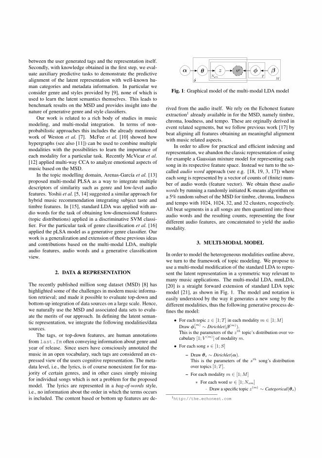
between the user generated tags and the representation itself.Secondly, with knowledge obtained in the first step, we eval-uate auxiliary predictive tasks to demonstrate the predictivealignment of the latent representation with well-known hu-man categories and metadata information. In particular weconsider genre and styles provided by [9], none of which isused to learn the latent semantics themselves. This leads tobenchmark results on the MSD and provides insight into thenature of generative genre and style classifiers.
Our work is related to a rich body of studies in musicmodeling, and multi-modal integration. In terms of non-probabilistic approaches this includes the already mentionedwork of Weston et al. [7]. McFee et al. [10] showed howhypergraphs (see also [11]) can be used to combine multiplemodalities with the possibilities to learn the importance ofeach modality for a particular task. Recently McVicar et al.[12] applied multi-way CCA to analyze emotional aspects ofmusic based on the MSD.
In the topic modelling domain, Arenas-Garcıa et al. [13]proposed multi-modal PLSA as a way to integrate multipledescriptors of similarity such as genre and low-level audiofeatures. Yoshii et al. [5, 14] suggested a similar approach forhybrid music recommendation integrating subject taste andtimbre features. In [15], standard LDA was applied with au-dio words for the task of obtaining low-dimensional features(topic distributions) applied in a discriminative SVM classi-fier. For the particular task of genre classification et al. [16]applied the pLSA model as a generative genre classifier. Ourwork is a generalization and extension of these previous ideasand contributions based on the multi-modal LDA, multipleaudio features, audio words and a generative classificationview.
2. DATA & REPRESENTATION
The recently published million song dataset (MSD) [8] hashighlighted some of the challenges in modern music informa-tion retrieval; and made it possible to evaluate top-down andbottom-up integration of data sources on a large scale. Hence,we naturally use the MSD and associated data sets to evalu-ate the merits of our approach. In defining the latent seman-tic representation, we integrate the following modalities/datasources.
The tags, or top-down features, are human annotationsfrom last.fm often conveying information about genre andyear of release. Since users have consciously annotated themusic in an open vocabulary, such tags are considered an ex-pressed view of the users cognitive representation. The meta-data level, i.e., the lyrics, is of course nonexistent for for ma-jority of certain genres, and in other cases simply missingfor individual songs which is not a problem for the proposedmodel. The lyrics are represented in a bag-of-words style,i.e., no information about the order in which the terms occursis included. The content based or bottom up features are de-
Fig. 1: Graphical model of the multi-modal LDA model
rived from the audio itself. We rely on the Echonest featureextraction1 already available in for the MSD, namely timbre,chroma, loudness, and tempo. These are orginally derived inevent related segments, but we follow previous work [17] bybeat aligning all features obtaining an meaningful alignmentwith music related aspects.
In order to allow for practical and efficient indexing andrepresentation, we abandon the classic representation of usingfor example a Gaussian mixture model for representing eachsong in its respective feature space. Instead we turn to the so-called audio word approach (see e.g. [18, 19, 3, 17]) whereeach song is represented by a vector of counts of (finite) num-ber of audio words (feature vector). We obtain these audiowords by running a randomly initiated K-means algorithm ona 5% random subset of the MSD for timbre, chroma, loudnessand tempo with 1024, 1024, 32, and 32 clusters, respectively.All beat segments in a all songs are then quantized into theseaudio words and the resulting counts, representing the fourdifferent audio features, are concatenated to yield the audiomodality.
3. MULTI-MODAL MODEL
In order to model the heterogeneous modalities outline above,we turn to the framework of topic modeling. We propose touse a multi-modal modification of the standard LDA to repre-sent the latent representation in a symmetric way relevant tomany music applications. The multi-modal LDA, mmLDA,[20] is a straight forward extension of standard LDA topicmodel [21], as shown in Fig. 1. The model and notation iseasily understood by the way it generates a new song by thedifferent modalities, thus the following generative process de-fines the model:
• For each topic z ∈ [1;T ] in each modality m ∈ [1;M ]
Draw φ(m)z ∼ Dirichlet(β(m)).
This is the parameters of the zth topic’s distribution over vo-cabulary [1;V (m)] of modality m.
• For each song s ∈ [1;S]
– Draw θs ∼ Dirichlet(α).This is the parameters of the sth song’s distributionover topics [1;T ].
– For each modality m ∈ [1;M ]
∗ For each word w ∈ [1;Nsm]
· Draw a specific topic z(m) ∼ Categorical(θs)
1http://the.echonest.com

0 50 100 150 2000
0.005
0.01
0.015
0.02
0.025
Tags sorted by avgNMI
avgN
MI
oldies (730)celtic (1439)mellow (380)blues rock (1530)bluegrass (129)humor (3906)female vocalist (37)world (1312)spoken word (2650)experimental (16)male vocalists (324)relaxing (1832)trance (1033)beautiful (34)90s (45)americana (543)house (544)love (238)chill (41)electro (136)
rap (46)singer−songwriter (269)smooth jazz (345)chillout (40)guitar (1177)funny (1951)electronica (481)indie (38)acoustic (382)dance (86)funk (58)alternative (96)spanish (342)christmas (206)worship (7744)christian rock (3411)latin (620)dancehall (1022)gospel (144)dub (603)
comedy (1944)jazz (347)country (527)blues (3)reggae (203)soul (158)new age (713)folk (379)female vocalists (70)electronic (138)hip−hop (42)rock (95)pop (5)rnb (55)instrumental (10)piano (365)christian (2232)ambient (39)hip hop (43)stand−up (1113)
Fig. 2: Normalized average mutual information (avgNMI) be-tween the latent representation defined by audio and lyrics forT = 128 topics and the 200 top-ranked tags. avgNMI is com-puted on the test set in each fold. The popularity of each tagis indicated in parenthesis.
· Draw a word w(m) ∼ Categorical(φ(m)
z(m))
A main characteristic of mmLDA is the common topicproportions for allM modalities in each song, s, and separateword-topic distributions p(w(m)|z) for each modality, wherez denotes a particular topic. Thus, each modality has its owndefinition of what a topic is in terms of its own vocabulary.
Model inference is performed using a collapsed Gibbssampler [22] similar to the standard LDA. The Gibbs sam-pler is run for a limited number of complete sweeps throughthe training songs, and the model state with the highest modelevidence within the last 50 iterations is regarded as the MAPestimate. From this MAP sample, point estimates of the topic-song distribution, p(z|s), and the modality, m, specific word-topic distribution, p(w(m)|z), can be computed based on theexpectations of the corresponding Dirichlet distributions.
Evaluation of model performance on a unknown test song,s∗, is performed using the procedure of fold-in [23, 24] bycomputing the point estimate of the topic distribution, p(z|s∗)for the new song, by keeping the all the word-topic countsfixed during a number of new Gibbs sweeps. Testing on amodality, not included in the training phase, requires a pointestimate of the word-topic distribution, p(w(m∗)|z), of theheld out modality, m∗, of the training data. This is obtainedby fixing the song-topic counts while updating the word-topiccounts for that specific modality. This is similar to the fold-inprocedure used for test songs.
4. EXPERIMENTAL RESULTS & DISCUSSION
4.1. Alignment
The first aim is to evaluate the latent representation’s align-ment with a human ’cognitive’ variable, which we previously
T032 T128 T5120
0.1
0.2
0.3
0.4
0.5
0.6
0.4
1±0
.01
3
0.4
2±0
.01
0
0.4
3±0
.00
7
0.3
3±0
.01
4
0.3
5±0
.01
5
0.3
6±0
.01
0
0.1
4±0
.00
8
0.1
4±0
.00
6
0.1
4±0
.00
7
0.1
8±0
.01
0
0.1
9±0
.00
7
0.1
9±0
.00
6
0.2
0±0
.00
8
0.2
2±0
.00
9
0.2
2±0
.00
9
Re
ca
ll
(a) Genre
T032 T128 T5120
0.1
0.2
0.3
0.4
0.5
0.2
8±0
.01
0
0.3
2±0
.00
7
0.3
4±0
.00
7
0.2
5±0
.01
4
0.2
9±0
.00
8
0.3
2±0
.00
9
0.1
1±0
.00
9
0.1
1±0
.00
4
0.0
9±0
.00
8
0.1
0±0
.00
4
0.1
1±0
.00
4
0.1
1±0
.00
4
0.1
2±0
.00
4
0.1
3±0
.00
4
0.1
3±0
.00
5
Re
ca
ll
(b) Style
Fig. 3: Classification accuracy for T ∈ {32, 128, 512}. Darkblue: Combined model; Light Blue: Tags; Green: Lyrics;Orange: Audio; Red: Audio+Lyrics.
argued could be the open vocabulary tags. We do this by in-cluding only the lower level modalities of audio and lyricswhen estimating the model. Then the normalized mutual in-formation between a single tag and the latent representations,i.e., the topics, is calculated for all the tags.
Thus for a single tag, wi(tag) we can compute the mutual
information between the tag and the topic distribution for aspecific song, s as:
MI(wi
(tag), z|s)
= (1)
KL(p(wi
(tag), z|s)||p(wi
(tag)|s)p (z|s)
),
where KL(·) denotes the Kullback-Leibler divergence. Wenormalize the MI to be in [0; 1], i.e,
NMI(wi
(tag), z|s)
= 2MI(wi
(tag), z|s)
H(wi
(tag)|s)
+H (z|s) ,
where H(·) denotes the entropy. Finally, we compute theaverage over all songs to arrive at the final measure ofalignment for a specific tag, given by avgNMI(wi
(tag)) =1S
∑s NMI
(wi
(tag), z|s).
Fig. 2 shows a sorted list of tags, where tags with highalignment with the latent representation have higher averageNMI (avgNMI). It is notable that the combination of the au-dio and lyrics modality, in defining the latent representation,seems to align well with genre-like and style-like tags. On thecontrary, emotional and period tags are relatively less alignedwith the representation. Also note that the alignment is notsimply a matter of the tag being the most popular as canbe seen from Fig. 2. Less popular tags are ranked higherby avgNMI than very popular tags, suggesting that some aremore specialized in terms of the latent representation thanothers.
The result gives merit to the idea of using genre and stylesas proxy for evaluating latent representation in comparisonwith other open vocabulary tags, since we - from lower levelfeatures, such as audio features and lyrics - can find latentrepresentations which align well with high-level, ’cognitive’aspects in an unsupervised way. This is in line with many

Blues Comedy/SpokenCountry Electronic Folk International Jazz Latin NewAge Pop/Rock RnB Rap Reggae Religious Vocal0
0.2
0.4
0.6
0.8
1
1.2
0.4
2±0.0
53
0.6
1±0.0
48
0.4
6±0.0
44
0.5
1±0.0
34
0.3
1±0.0
32
0.1
9±0.0
36
0.3
7±0.0
48
0.4
2±0.0
42
0.5
5±0.0
47
0.4
1±0.0
40
0.5
0±0.0
41
0.4
3±0.0
38
0.5
1±0.0
48
0.3
9±0.0
32
0.2
5±0.0
41
0.3
9±0.0
38
0.4
3±0.0
51
0.3
7±0.0
51
0.4
6±0.1
98
0.2
3±0.0
33
0.1
5±0.0
24
0.3
2±0.0
38
0.2
4±0.0
34
0.3
9±0.0
35
0.5
4±0.2
21
0.4
1±0.0
29
0.2
8±0.0
26
0.4
1±0.0
39
0.2
8±0.0
35
0.2
9±0.2
90
0.1
1±0.2
90
0.0
3±0.0
16
0.1
1±0.0
27
0.2
8±0.4
40
0.0
6±0.0
17
0.0
5±0.0
15
0.2
9±0.4
66
0.2
8±0.0
23
0.2
9±0.4
63
0.0
8±0.0
24
0.0
9±0.0
12
0.1
7±0.0
27
0.0
4±0.0
13
0.1
7±0.0
38
0.0
4±0.0
11
0.1
3±0.0
23
0.4
9±0.0
41
0.1
5±0.0
36
0.1
9±0.0
45
0.1
1±0.0
22
0.0
3±0.0
13
0.1
2±0.0
26
0.0
4±0.0
20
0.3
8±0.0
42
0.2
6±0.0
37
0.1
1±0.0
26
0.2
4±0.0
44
0.2
4±0.0
30
0.0
7±0.0
22
0.2
6±0.0
24
0.1
1±0.0
23
0.4
5±0.0
50
0.2
1±0.0
29
0.1
9±0.0
40
0.1
1±0.0
28
0.0
5±0.0
19
0.1
2±0.0
33
0.3
5±0.0
29
0.3
9±0.0
38
0.2
8±0.0
25
0.1
6±0.0
49
0.2
9±0.0
34
0.2
0±0.0
27
0.1
5±0.0
41
0.2
2±0.0
20
Recall
Fig. 4: Dark blue: Combined model, Light Blue: Tags, Green: Lyrics, Orange: Audio, Red: Audio+Lyrics, genre, T = 128.
Predicted class
Tru
e c
lass
Blues
Comedy/Spoken
Country
Electronic
Folk
International
Jazz
Latin
NewAge
Pop/Rock
RnB
Rap
Reggae
Religious
Vocal
0.1
0.2
0.3
0.4
0.5
0.6
(a) Combined Model
Predicted class
Tru
e c
lass
Blues
Comedy/Spoken
Country
Electronic
Folk
International
Jazz
Latin
NewAge
Pop/Rock
RnB
Rap
Reggae
Religious
Vocal
0.1
0.2
0.3
0.4
0.5
(b) Tag Model
Predicted class
Tru
e c
lass
Blues
Comedy/Spoken
Country
Electronic
Folk
International
Jazz
Latin
NewAge
Pop/Rock
RnB
Rap
Reggae
Religious
Vocal
0.05
0.1
0.15
0.2
0.25
0.3
(c) Lyrics Model
Predicted class
Tru
e c
lass
Blues
Comedy/Spoken
Country
Electronic
Folk
International
Jazz
Latin
NewAge
Pop/Rock
RnB
Rap
Reggae
Religious
Vocal0.05
0.1
0.15
0.2
0.25
0.3
0.35
0.4
0.45
(d) Audio Model
Fig. 5: Confusion matrices for genre and 128 topics. The color level indicates the classification accuracy.
studies in music informatics on western music (see e.g. [25,26, 27]) which indicate coherence between genre and tag cat-egories and cognitive understanding of music structure. Insummary, the ranking of tag alignment using our modelingapproach on the MSD provides some evidence in favor ofsuch coherence.
4.2. Prediction
Given the evidence presented for genre and style being therelatively most appropriate human categories, our second aimis to evaluate the predictive performance of the multi-modalmodel for genre and style, and we turn to the recently pub-lished extension of the MSD [9] for reference test/train splitsand genre and style labels. In particular, we use the balancedsplits defined in [9].
For the genre case, this results in 2000 labeled examplesper genre and 15 genres, thus resulting in 30, 000 songs. Weestimate the predictive genre performance by 10-fold cross-validation. Fig. 4 shows the per-label classification accuracy(perfect classification equals 1). The total genre classificationperformance is illustrated in Fig. 3a. The corresponding re-sult for style classification, based on a total of 50, 000 labeledexamples, is shown in Fig. 3b. Both results are generated us-ing T = 128 topics, 2000 Gibbs sweeps and predicting usingthe MAP estimate from the Gibbs sampler.
We first note that the combination of all modalities per-forms the best and significantly better than random as seenfrom Fig. 3, which is encouraging, and support the multi-modal approach. It is furthermore noted that the tag modalityis able to perform very well. This indicates that despite thepossibly noisy user expressed view, the model is able to findstructure in line with the taxonomy defined in the referencelabels of [9]. More interesting is perhaps the audio and lyric
modalities and the combination of the two. This shows thatlyrics performs the worst for genre, possibly due to the miss-ing data in some tracks, while the combination is significantlybetter. For style there is no significant difference between au-dio and lyrics.
Looking at the genre specific performance in Fig. 4 wefind a significant difference between the modalities. It ap-pears that the importance of the modalities is partly in linewith the fundamentally different characteristics of each spe-cific genre. For example ’latin’ is driven by very characteris-tic lyrics. Further insight can be obtained by considering theconfusion matrices which show some systematic pattern of er-ror in the individual modalities, whereas the combined modelshows a distinct diagonal structure, highlighting the benefitsof multi-modal integration.
5. CONCLUSION
In this paper, we proposed the multi-way LDA as a flexiblemodel for analyzing and modeling multi-modal and hetero-geneous music data in a large scale setting. Based on theanalysis of tags and latent representation, we provided evi-dence for the common assumption that genre may be an ac-ceptable proxy for cognitive categorization of (western) mu-sic. Finally, we demonstrated and analyzed the predictive per-formance of the generative model providing benchmark resultfor the Million Song Dataset, and a genre dependent perfor-mance was observed. In our current research, we are lookingat purely supervised topic models trained for, e.g. genre pre-diction. In order to address truly multi-modal and multi-taskscenarios such as [7], we are currently pursuing an extendedprobabilistic framework that include correlated topic models[28], multi-task models [29], and non-parametric priors [30].
6. REFERENCES
[1] L.K. Hansen, P. Ahrendt, and J. Larsen, “Towards cognitivecomponent analysis,” in AKRR05-International and Interdis-ciplinary Conference on Adaptive Knowledge Representationand Reasoning, 2005.
[2] C. Xu, N.C. Maddage, and X. Shao, “Musical genre classi-fication using support vector machines,” IEEE InternationalConference on Acoustics, Speech and Signal Processing, pp.429–432, 2003.
[3] M. Hoffman, D. Blei, and P. Cook, “Easy as CBA: A simpleprobabilistic model for tagging music,” Proc. of ISMIR, pp.369–374, 2009.
[4] F. Pachet and J.J. Aucouturier, “Improving timbre similarity:How high is the sky?,” Journal of negative results in speechand audio, pp. 1–13, 2004.
[5] Y. Kazuyoshi, M. Goto, K. Komatani, R. Ogata, and H.G.Okuno, “Hybrid collaborative and content-based music rec-ommendation using probabilistic model with latent user pref-erences,” in Proceedings of the 7th International Conferenceon Music Information Retrieval (ISMIR, 2006, pp. 296–301.
[6] E. Law, B. Settles, and T. Mitchell, “Learning to tag fromopen vocabulary labels,” Machine Learning and KnowledgeDiscovery in Databases, pp. 211–226, 2010.
[7] J. Weston, S. Bengio, and P. Hamel, “Multi-Tasking with JointSemantic Spaces for Large- Scale Music Annotation and Re-trieval Multi-Tasking with Joint Semantic Spaces for Large-Scale Music Annotation and Retrieval,” Journal of New MusicResearch, , no. November 2012, pp. 37–41, 2011.
[8] T. Bertin-Mahieux, D.P.W. Ellis, B. Whitman, and P. Lamere,“The million song dataset,” in Proceedings of the 12th Inter-national Conference on Music Information Retrieval (ISMIR2011), 2011.
[9] A. Schindler, R. Mayer, and A. Rauber, “Facilitating com-prehensive benchmarking experiments on the million songdataset,” in 13th International Conference on Music Informa-tion Retrieval (ISMIR 2012). 2012.
[10] B. McFee and G. R. G. Lanckriet, “Hypergraph models ofplaylist dialects,” in Proceedings of the 13th InternationalSociety for Music Information Retrieval Conference, FabienGouyon, Perfecto Herrera, Luis Gustavo Martins, and MeinardMuller, Eds. 2012, pp. 343–348, FEUP Edicoes.
[11] J. Bu, S. Tan, C. Chen, C. Wang, H. Wu, L. Zhang, and X. He,“Music Recommendation by Unified Hypergraph: CombiningSocial Media Information and Music Content,” pp. 391–400,2010.
[12] M. Mcvicar and T. de Bie, “CCA and a Multi-way Exten-sion for Investigating Common Components between Audio ,Lyrics and Tags .,” in CMMR, 2012, number June, pp. 19–22.
[13] J. Arenas-Garcıa, A. Meng, K.B. Petersen, T. Lehn-Schiøler,L.K. Hansen, and J. Larsen, Unveiling Music Structure ViaPLSA Similarity Fusion, pp. 419–424, IEEE, 2007.
[14] K. Yoshii and M. Goto, “Continuous pLSI and smoothing tech-niques for hybrid music recommendation,” International Soci-ety for Music Information Retrieval Conference, pp. 339–344,2009.
[15] S. K., S. Narayanan, and S. Sundaram, “Acoustic topic modelfor audio information retrieval,” pp. 2–5, 2009.
[16] Zhi Zeng, Shuwu Zhang, Heping Li, W. Liang, and HaiboZheng, “A novel approach to musical genre classification usingprobabilistic latent semantic analysis model,” in IEEE Inter-national Conference on Multimedia and Expo (ICME), 2009,
2009, pp. 486–489.[17] T. Bertin-Mahieux, “Clustering beat-chroma patterns in a large
music database,” in International Society for Music Informa-tion Retrieval Conference, 2010.
[18] Y. Cho and L.K. Saul, “Learning dictionaries of stable autore-gressive models for audio scene analysis,” Proceedings of the26th Annual International Conference on Machine Learning -ICML ’09, pp. 1–8, 2009.
[19] K. Seyerlehner, G. Widmer, and P. Knees, “Frame level audiosimilarity-a codebook approach,” Conference on Digital AudioEffects, pp. 1–8, 2008.
[20] D.M. Blei and M.I. Jordan, “Modeling annotated data,” Pro-ceedings of the 26th annual international ACM SIGIR confer-ence on Research and development in informaion retrieval, pp.127–134, 2003.
[21] D. M. Blei, A. Ng, and M. Jordan, “Latent Dirichlet alloca-tion,” The Journal of Machine Learning Research, vol. 3, pp.993–1022, 2003.
[22] T.L. Griffiths and M. Steyvers, “Finding scientific topics.,”Proceedings of the National Academy of Sciences of the UnitedStates of America, pp. 5228–35, Apr. 2004.
[23] H.M. Wallach, I. Murray, Ruslan Salakhutdinov, andD. Mimno, “Evaluation methods for topic models,” Proceed-ings of the 26th Annual International Conference on MachineLearning - ICML ’09, , no. d, pp. 1–8, 2009.
[24] T. Hofmann, “Probabilistic latent semantic analysis,” Proc. ofUncertainty in Artificial Intelligence, UAI, p. 21, 1999.
[25] J.H. Lee and J..S Downie, “Survey of music information needs,uses, and seeking behaviours: Preliminary findings,” in Proc.of ISMIR, 2004, pp. 441–446.
[26] J. Frow, Genre, Routledge, New York, NY, USA, 2005.[27] E. Law, “Human computation for music classification,” in Mu-
sic Data Mining, T. Li, M. Ogihara, and G. Tzanetakis, Eds.,pp. 281–301. CRC Press, 2011.
[28] S. Virtanen, Y. Jia, A. Klami, and T. Darrell, “Factorized Multi-Modal Topic Model,” auai.org, 2010.
[29] A. Faisal, J. Gillberg, J. Peltonen, G. Leen, and S. Kaski,“Sparse Nonparametric Topic Model for Transfer Learning,”dice.ucl.ac.be.
[30] Y.W. Teh, M.I. Jordan, M.J. Beal, and D.M. Blei, “Hierarchi-cal dirichlet processes,” Journal of the American StatisticalAssociation, vol. 101, 2004.

156
Appendix I
Personalized Audio System -a Bayesian Approach
Jens Brehm Nielsen, Bjørn Sand Jensen, Toke Jansen Hansen and Jan Larsen,Personalized Audio System - a Bayesian Approach, 135th AES Convention,2013.
Note: Only a pre-print of the published paper is included, the published versioncan be found via the publisher, http://www.aes.org/e-lib/browse.cfm?elib=17048.

158 Appendix I

Personalized Audio Systems
- a Bayesian Approach
Jens Brehm Nielsen (1,2), Bjørn Sand Jensen (1),Toke Jansen Hansen (1), and Jan Larsen (1)
(1) Technical University of Denmark, DTU Compute, Matematiktorvet 303B, 2800Lyngby, Denmark
(2) Widex A/S, Nymøllevej 6, 3540 Lynge, Denmark
Abstract
Modern audio systems are typically equipped with several user-adjustableparameters unfamiliar to most users listening to the system. To obtainthe best possible setting, the user is forced into multi-parameter optimiza-tion with respect to the users’s own objective and preference. To addressthis, the present paper presents a general inter-active framework for per-sonalization of such audio systems. The framework builds on BayesianGaussian process regression in which a model of the users’s objective func-tion is updated sequentially. The parameter setting to be evaluated in agiven trial is selected by model-based sequential experimental design. AGaussian process model is proposed which incorporates correlation amongparticular parameters providing better modeling capabilities compared toa standard model. A five-band equalizer is considered for demonstra-tion purposes, in which the parameters are optimized using the proposedframework. Twelve test subjects obtain a personalized setting with theframework, and these settings are significantly preferred to those obtainedwith random experimentation.
1 Introduction
The ever increasing number of features and processing possibilities in manymodern multimedia systems, such as personal computers, mobile phones, hear-ing aids and home entertainment systems, has made it possible for users tocustomize these systems significantly. A downside in this trend is the largenumber of user-adjustable parameters which makes it a daunting and complextask to actually adjust/optimize the systems optimally. This is because usershave to navigate in a high-dimensional parameter space, which makes it ex-tremely difficult for users to find even a local optimum. For audio systems, theoptimization is further complicated by perceptual and cognitive aspects of thehuman auditory and cognitive system, which result in a significant spread in
1

10 1000 10000−15
−10
−5
0
5
10
15
Frequency [Hz]
Gai
n [d
B]
!1
!0.5
0
0.5
1
0
5
10!4
!2
0
2
4
x
Trained GP
t
f(x,t)
(1)
(2)
(3)
Figure 1: A conceptual overview of the interactive system. At step (1) we drawa new EQ from the current estimate of the user’s objective function. Next, atstep (2) this particular EQ is associated with a ball, in this case number eight, inthe visualized user interface. Finally, after the user has rated the new EQ, theobjective function is updated to reflect current positions of all previous balls,this update occurs at step (3). We emphasize that the user at any time mayselect between previously sampled EQ by clicking the balls, making the currentsong play through the newly selected EQ.
users’s opinions concerning the adjustment of a particular system. It is there-fore of great interest to find and evaluate fast and flexible tools for robustlyoptimizing user-adjustable parameters, with the aim to rapidly obtain a trulypersonalized audio system setting.
Prime examples of complex audio systems are hearing aids, where hundredsof parameters make up a unique and personal experience. It is therefore nat-ural that this field has considered ways to learn an optimal setting based onpreference (Kuk et. al. [8] and Baskent et. al. [1]), although these are currentlybased on non-probabilistic methods. Recently—and the closest related to ourapproach—Birlutiu et. al. [4, 3] have proposed two probabilistic approachesdriven mainly by a multi-task formulation utilizing the information transferamong users, to learn a complete preference model accounting for all preferencerelations. For the purpose of optimizing parameters, it is not efficient to learna complete model over a high-dimensional parameter space, because the modelis only required to be accurate around possible optimal parameters.
In audio reproduction systems—like home entertainment and professionalmixing equipment—preference learning approaches are relatively unknown, de-spite the clear evidence that personalization may be beneficial in for exampleequalization (Paterson [11] and Zhang et. al. [18]). Existing approaches such asReed [13], Pardo et. al. [10], and Sabin et. al. [14], are based on non-probabilisticapproaches, thus neglecting the highly stochastic nature of perceptual responses.
2

In this work we focus on audio reproduction systems and the outlined taskof optimizing multiple parameters in such systems for an individual user listen-ing to the output of the system. For this purpose, we propose and consider acombination of robust Bayesian modeling, an engaging user interface for userfeedback and global optimization techniques (active learning) in an interactiveloop visualized in Fig. 1. The loop constitutes a general framework where theinherent uncertainty in user feedback is addressed from a Bayesian viewpointin which the belief in the user’s (unknown) objective function is modeled with(warped) Gaussian process (GP) regression [15]. The framework uses an intu-itive and simple graphical user interface for obtaining user ratings, which allowsthe user to listen to previously rated settings thus serving as anchors/referencesfor future ratings. In contrast to standard practice, we do however not only al-low the user to listen to previous settings, but we also allow the user to changeall the ratings of previous settings, if for some reason a new setting would changee.g. the span of the scale. This is possible, since we are constantly updating ourregression model to reflect the belief about the user’s objective function giventhe ratings obtained so far. Finally, we propose to use a sequential optimiza-tion technique to rapidly find a (possibly local) optimum of the user’s objectivefunction. The sequential design takes advantage of the Bayesian formulationby including the belief about the user’s objective function. This significantlyreduces the required number of settings that the user should rate in order tofind an optimum.
We furthermore consider the fact that certain parameters may be correlatedwith respect to the user’s objective. An example could be the compressionratio, the attack time and the release time in a compressor. To exploit suchcorrelation and obtain better modeling capabilities, we suggest a specific modelwhich assumes correlation between specific input parameters.
To demonstrate the potential of the framework for personal audio systemoptimization, we use a five-band constant-Q equalizer (EQ) as the running ex-ample, because the parameters (gains) in an EQ is something that we (as profes-sionals) more or less all can relate to. We are aware that any audio-engineeringprofessional will probably be able to quickly tune the five parameters of the EQto his own objective. However, this is actually not a very typical scenario. Typ-ically, users of home entertainment systems are untrained, and thus, have verylittle intuition about the parameters that they have the opportunity to tuneand close to no intuition at all about the interplay between parameters. Hencewith for instance five parameters controlling a virtual surround sound systemwith virtual base enhancement, most users would seek an optimal setting usingtrial and error (random experimentation). This is the premises in which the EQexample should be considered and the EQ is just convenient for demonstrationpurposes.
Through model comparison, we first show that the model with assumed cor-relation between input parameters improves the modeling capabilities comparedto a traditional GP model without assumed correlation. The analysis is per-formed on real-world data, where 21 test subjects have rated different randomlychosen settings of the EQ. Even for this EQ with relative few bands—which is
3

thus perceptually well separated—we would expect the gains in adjacent bandsto be somewhat correlated with regards to the user’s objective. Secondly, weevaluate the usefulness of the entire framework in a real-world experiment wherepersonalization of the EQ have been conducted for twelve test subjects. As theEQ has over fifty-nine thousands unique settings, the hypothesis is that thepreferred setting will be hard to find (for the typically untrained user) with-out an efficient sequential design approach and correspondingly good modelingcapabilities. The results from the real-world listening experiments focusing onthe statistical difference between random experimentation and sequential exper-imental design, show a clear advantage of the sequential design approach.
Our contribution is thus three fold: First in Sec. 2, we propose a generalpersonalization framework with an intuitive user interface (Sec. 2.3), a princi-pled modeling approach using warped Gaussian processes extended to expectcorrelation between adjacent input parameters (Sec. 2.1) and a sequential designapproach (Sec. 2.2). Secondly in Sec. 3.2, we show that the GP model extensionprovides better modeling capabilities for our specific purpose. Thirdly, we eval-uate the entire framework by a listening experiment in a real-world interactivescenario and outline the results in Sec. 3.3. A discussion is provided in Sec. 4and the paper is concluded in Sec. 5.
2 Personalization Framework
The proposed personalization framework uses an interactive loop to discover theuser’s preferred setting of a particular audio system, where we as an exampleuse the EQ. The interactive loop is visualized in Fig. 1. The loop can conceptu-ally be divided into three parts: a preference modeling part, a sequential designpart and an interface part. The preference modeling part presents how a user’sobjective function over EQ settings is learned based on user ratings. The se-quential design part covers how to choose new EQ settings to be rated based onwhat the model currently predicts. Finally, the interface part covers the designof the graphical user interface, such that it is both intuitive and easy to use forthe users. The three parts are described in the following three sections.
2.1 Preference Modeling
We represent each system setting as a d = 5 dimensional vector of parameters,x = [x1, ..., xd]
>. Next, we assumed that the user’s objective is an unobservedreal-valued stochastic function (or process), such that each unique setting xi hasa corresponding real-valued function value, f(xi), expressing the user’s prefer-ence for the particular setting. This function is to be learned—and subsequentlymaximized—trough a number of experiments where we observe the user’s ex-pressed preference by a rating on a bounded scale, y ∈ ]0; 1[, where 0 is Bad and1 is Good (see interface (2) on Fig. 1). At some point the user has evaluated nsuch distinct system settings xi ∈ X collected in X = {xi|i = 1, ..., n}, with arelated set of n responses denoted Y = {yi|i = 1, ..., n}.
4

We model the function mapping from settings, xi, to ratings, yi, by a so-called warped Gaussian process [15]. A standard Gaussian process (GP) is astochastic process defined as a collection of random variables, any finite subsetof which must have a joint Gaussian distribution [12]. In effect, the GP isplaced as a prior over any finite set of functional values f = [f1, f2, ..., fn]>,where fi = f(xi), resulting in a finite multivariate Gaussian distribution overthe set as f |X ∼ N (0,KXX), where each element of the covariance matrix KXX
is given by a covariance function k(·, ·) such that [KXX]i,j = k(xi,xj). The GPprior can be used in non-parametric Bayesian regression frameworks where thelikelihood function can be parameterized by a smooth and continuous functionf(·).
However, our regression setup is special due to the bounded nature of the rat-ings. We therefore use a warped Gaussian process in which the original ratings inY are transformed into a form where the data is modeled by a traditional Gaus-sian noise model [12, Chapter 2]. Several warping functions would apply, buta natural choice is the inverse cumulative Gaussian (probit) Φ−1(·)—with zeromean and unity variance—such that observations are warped as zi = Φ−1(yi).
The final model is defined by,
σs|θs ∼ U(0,∞)
σ`|θ` ∼ U(0,∞)
σ|θ` ∼ U(0,∞)
fi|σs, σ` ∼ GP(m (xi) , k (xi, ·)σs,σ`
)
zi|fi ∼ N (fi, σ) (1)
zi = Φ−1 (yi) , (2)
where σ` is the length scale of the covariance function, σs is the standard de-viation of the latent function, and σ is the noise standard deviation (in latentspace). U(a, b) denotes a uniform hyper prior on the open interval from a tob, i.e. an improper and non-informative prior. Alternatively, so-called weakly-informative hyper priors would apply—especially over the length scale σ`—such as the half-student-t hyper prior [5, 16], which could be applied to providea more robust inference and prediction scheme avoiding the GP model to fithyperplanes with only few observations. We note that the observation noise, σ,can be included in the covariance function.
Given this model, the main question remains regarding the covariance (orkernel) function, which effectively defines the smoothness of the function. Weconsider two covariance functions based on the general form of the squaredexponential kernel [12]
k (xi,xj)
= σs exp
(− 1
σ`(xi − xj)
>Λ−1 (xi − xj)
).
(3)
5

In the first case, Λ is the identity matrix leading to the well-known (isotropic)
squared exponential covariance function kiso (xi,xj) = σs exp(− 1σ`‖xi − xj‖2
).
In the second case, Λ is a general positive semi-definite matrix defining a cor-relation between parameters (input space) as explicit prior information. Herewill denote this variant as the Mahalanobis covariance function1, kmah (xi,xj)and set
Λmah =
1 0.5 0.2 0 00.5 1 0.5 0.2 00.2 0.5 1 0.5 0.20 0.2 0.5 1 0.50 0 0.2 0.5 1
. (4)
The effect of the two options on the EQ example will be evaluated with referenceto the standard case as iso and the Mahalanobis case as mah.
We turn to a standard GP inference scheme [12] in which the covariance andlikelihood parameters, σs, σ`, σ, are approximated by point estimates by maxi-mizing the marginal likelihood (or evidence) using a BFGS method and wherethe posterior p(f |Y,X) is analytical tractable [15]. For the BFGS methods, theparameters are always initialized as σs = 1, σ` = 1, σ = 1. The predictive meanand (co)variance of the latent function, E(f∗) and V(f∗), are given in standardform [12] as
E {f∗} = K>XX∗[KXX + σ2
i I]−1
Φ−1 (Y) (5)
V {f∗} = KX∗X∗ −K>XX∗[KXX + σ2
i I]−1
KXX∗ (6)
where KAB is the kernel matrix containing either evaluations between traininginputs, A = B = X, test inputs, A = B = X∗, or between training and testinputs, A = X,B = X∗.
The predictive distribution and in particular the predictive uncertainty is aclear advantage of the probabilistic GP framework, since the predictive meanand predictive (co)variance can be used to determine the information gain inincluding a new candidate point into the model as considered in the next section.
2.2 Sequential Experimental Design
Classical experimental designs such as Latin Squares or random experimentation[9] become increasingly infeasible in high dimensions. As an alternative, wepropose to use sequential design approaches which, by greedy selection of themost informative next sample, potentially achieve much faster convergence thanfixed designs [7].
The main purpose is to define a selection criterion which finds the optimalof the (unknown) objective function. The applied criterion is a slightly modified
1Sometimes also referred to as a anisotropic (squared exponential) covariance functions[12].
6
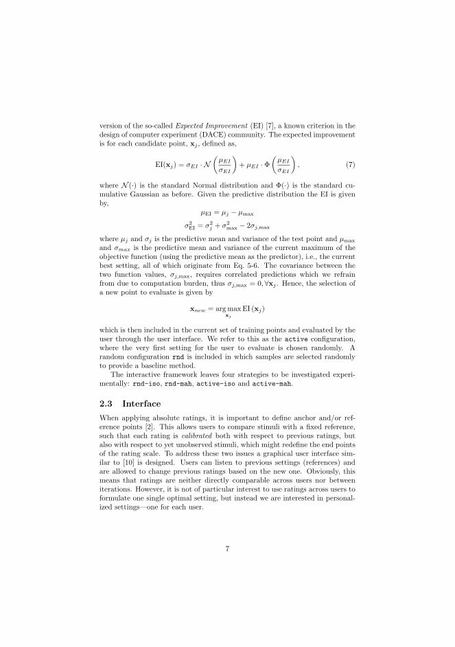
version of the so-called Expected Improvement (EI) [7], a known criterion in thedesign of computer experiment (DACE) community. The expected improvementis for each candidate point, xj , defined as,
EI(xj) = σEI · N(µEIσEI
)+ µEI · Φ
(µEIσEI
), (7)
where N (·) is the standard Normal distribution and Φ(·) is the standard cu-mulative Gaussian as before. Given the predictive distribution the EI is givenby,
µEI = µj − µmax
σ2EI = σ2
j + σ2max − 2σj,max
where µj and σj is the predictive mean and variance of the test point and µmax
and σmax is the predictive mean and variance of the current maximum of theobjective function (using the predictive mean as the predictor), i.e., the currentbest setting, all of which originate from Eq. 5-6. The covariance between thetwo function values, σj,max, requires correlated predictions which we refrainfrom due to computation burden, thus σj,max = 0,∀xj . Hence, the selection ofa new point to evaluate is given by
xnew = arg maxxj
EI (xj)
which is then included in the current set of training points and evaluated by theuser through the user interface. We refer to this as the active configuration,where the very first setting for the user to evaluate is chosen randomly. Arandom configuration rnd is included in which samples are selected randomlyto provide a baseline method.
The interactive framework leaves four strategies to be investigated experi-mentally: rnd-iso, rnd-mah, active-iso and active-mah.
2.3 Interface
When applying absolute ratings, it is important to define anchor and/or ref-erence points [2]. This allows users to compare stimuli with a fixed reference,such that each rating is calibrated both with respect to previous ratings, butalso with respect to yet unobserved stimuli, which might redefine the end pointsof the rating scale. To address these two issues a graphical user interface sim-ilar to [10] is designed. Users can listen to previous settings (references) andare allowed to change previous ratings based on the new one. Obviously, thismeans that ratings are neither directly comparable across users nor betweeniterations. However, it is not of particular interest to use ratings across users toformulate one single optimal setting, but instead we are interested in personal-ized settings—one for each user.
7
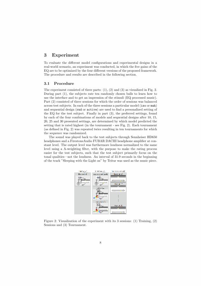
3 Experiment
To evaluate the different model configurations and experimental designs in areal-world scenario, an experiment was conducted, in which the five gains of theEQ are to be optimized by the four different versions of the proposed framework.The procedure and results are described in the following section.
3.1 Procedure
The experiment consisted of three parts: (1), (2) and (3) as visualized in Fig. 2.During part (1), the subjects rate ten randomly chosen balls to learn how touse the interface and to get an impression of the stimuli (EQ processed music).Part (2) consisted of three sessions for which the order of sessions was balancedacross test subjects. In each of the three sessions a particular model (iso or mah)and sequential design (rnd or active) are used to find a personalized setting ofthe EQ for the test subject. Finally in part (3), the preferred settings, foundby each of the four combinations of models and sequential designs after 10, 15,20, 25 and 30 presented settings, are determined by which model predicted thesetting that is rated highest (in the tournament - see Fig. 2). Each tournament(as defined in Fig. 2) was repeated twice resulting in ten tournaments for whichthe sequence was randomized.
The sound was played back to the test subjects through Sennheiser HD650headphones and a FirestoneAudio FUBAR DACIII headphone amplifier at con-stant level. The output level was furthermore loudness normalized to the samelevel using a A-weighting filter, with the purpose to make the rating processeasier for the test subjects, such that the test subject primarily focus on thetonal qualities—not the loudness. An interval of 31.9 seconds in the beginningof the track ”Sleeping with the Light on” by Teitur was used as the music piece.
Figure 2: Visualization of the experiment with its 3 sessions: (1) Training, (2)Sessions and (3) Tournament.
8
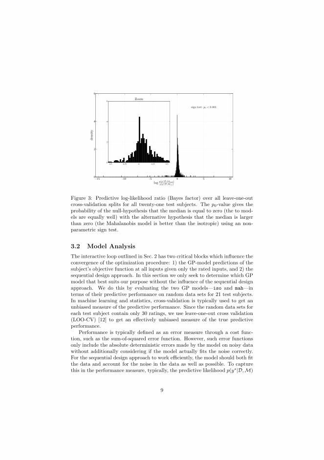
−15 −10 −5 0 5 100
2
4
6
log p(y∗|D,Mmah)p(y∗|D,Miso)
den
sity
sign test: p0 < 0.001
−0.5 −0.25 0 0.25 0.50
2
4
6Zoom
Figure 3: Predictive log-likelihood ratio (Bayes factor) over all leave-one-outcross-validation splits for all twenty-one test subjects. The p0-value gives theprobability of the null-hypothesis that the median is equal to zero (the to mod-els are equally well) with the alternative hypothesis that the median is largerthan zero (the Mahalanobis model is better than the isotropic) using an non-parametric sign test.
3.2 Model Analysis
The interactive loop outlined in Sec. 2 has two critical blocks which influence theconvergence of the optimization procedure: 1) the GP-model predictions of thesubject’s objective function at all inputs given only the rated inputs, and 2) thesequential design approach. In this section we only seek to determine which GPmodel that best suits our purpose without the influence of the sequential designapproach. We do this by evaluating the two GP models—iso and mah—interms of their predictive performance on random data sets for 21 test subjects.In machine learning and statistics, cross-validation is typically used to get anunbiased measure of the predictive performance. Since the random data sets foreach test subject contain only 30 ratings, we use leave-one-out cross validation(LOO-CV) [12] to get an effectively unbiased measure of the true predictiveperformance.
Performance is typically defined as an error measure through a cost func-tion, such as the sum-of-squared error function. However, such error functionsonly include the absolute deterministic errors made by the model on noisy datawithout additionally considering if the model actually fits the noise correctly.For the sequential design approach to work efficiently, the model should both fitthe data and account for the noise in the data as well as possible. To capturethis in the performance measure, typically, the predictive likelihood p(y∗|D,M)
9

of the unseen data points y∗ given the model M and the observed data D isused.
A proper Bayesian and statistical way of comparing two models [17, 6] isto compare the (predictive) likelihood ratio p(y∗|D,Mmah)/p(y∗|D,Miso) be-tween the two different models—mah and iso. This is also referred to as theBayes factor [6]. A (log) Bayes factor larger than zero favors the model denotedin the nominator, whereas a (log) Bayes factor less than zero favors the modelin the denominator.
For each of the 21 random data sets—one for each test subject— LOO-CV isused and the (log) Bayes factor is calculated for each LOO-CV split. This givesa total of 21×30 Bayes factor estimates shown in a histogram in Fig. 3. We seethat on average, the mah model performs the best probabilistic predictions oftest subjects’s individual ratings and thus appears to be the most suitable modeldue to the assumed correlation between adjacent parameters. A non-parametricsign test shows that this is significant (sample size of 630).
3.3 Sequential Design Analysis
The results are summarized in Fig. 4(a). The illustrated p0-values gives thesignificance level for which the null-hypothesis, that the total number of activewins is equal to the total number of random wins at each tournament point(#examples), can be accepted.
Averaged across test subjects and repetitions, the sequential design is signifi-cantly better than random design after any given number of examples, as shownby the p0–values. This is without distinguishing between the two applied covari-ance functions. It demonstrates the potential of the Bayesian model and activelearning methods in audio applications. It is furthermore noted that a standardfixed design will approximate the random configuration in this high-dimensionalspace.
The second aspect is if the more informative Mahalanobis (mah) prior resultsin a more accurate model with only a few ratings available. This is generallynot the case, although the specific Mahalanobis model possesses better gen-eralization capabilities compared to the isotropic model as shown in Sec. 3.2.
4 Discussion and Future Work
The results presented in this paper has focused first on verifying that the pro-posed Mahanolobis model is suitable in this context, and secondly, demonstrat-ing that the sequential design approach actually performs as expected (and bet-ter than random). There are however many possibilities for further evaluationand development.
In regards to the specific prior, we believe despite the lack of evidence inthe present paper, that the Mahalanobis covariance function will be found suit-able in several audio applications—including the EQ example used here. We
10

10 15 20 25 300
10
20
30
40
50
60
#examples
%wins
p0 < 0.011
p0 < 0.001
p0 < 0.076
p0 < 0.032
p0 < 0.001
rnd-iso rnd-mah active-iso active-mah
(a) Learning Curve
101
102
103
104
−15
−10
−5
0
5
10
15
Freq [Hz]
Gain[dB]
subject 2 - random
101
102
103
104
−15
−10
−5
0
5
10
15
Freq [Hz]
Gain[dB]
subject 2 - active-mah
101
102
103
104
−15
−10
−5
0
5
10
15
Freq [Hz]
Gain[dB]
subject 2 - active-iso
(b) Ratings
Figure 4: (a): The percentage of times the predicted preferred setting by eachof the four models wins over the other models across test subjects at each ofthe five tournament points. The p0-values is for accepting the null-hypothesisthat the two active sequential design approaches is equal to the two randomapproaches using a binomial test. (b): Actual ratings of different EQ settingsfrom the three Sessions for test subject 2. The EQ curves are the imposed gainand the color and thickness of the EQ curves both indicate the rating, wherethink/dark black is a good ratings (y → 1) and thin/light gray is a bad ratings(y → 0).
speculate that at least two additions would improve the performance of theMahalanobis model in the suggested framework. Firstly, the modeling capa-bilities could be improved by a parametrization of the correlation structure inthe Mahalanobis kernel by a small set of parameters, which could then be in-
11

ferred from data. The latter is easily accomplished in the GP framework byevidence maximization. Secondly, the sequential design criterion (Sec. 2.2) doesnot in its current form fully exploit the correlation between predictive functionvalues for different settings. To include this correlation the covariance matrixbetween all unique settings must be calculated. Calculating these is currentlycomputational infeasible. To overcome this and exploit the modeled correlationin the sequential design criterion, a greedy-gradient approach is currently beingdeveloped and tested with regards to find a (possible local) optimum of the(correlated) EI.
The Gaussian process modeling approach will in general benefit from theaddition of weakly informative hyper-priors over especially the length scale pa-rameter, σ`. This will result in a more robust inference scheme in which unreal-istic hyper-plane predictions of the user’s objective function would be avoided,thus aiding the sequential design. This is currently being introduced into themodeling framework.
The current evaluation is based on an absolute paradigm with adjustableanchors in terms of previous ratings. For the user, it can however be quite de-manding to keep track of all ratings, when there are several items (balls) present,which leads to inconsistent ratings. The GP based personalization frameworkis easily extendable with other paradigms such as pairwise comparisons or moregeneral ranking based approaches. It is speculated that a more robust paradigm(with respect to user feedback) may further aid the optimization process.
Finally, it is the ambition to evaluate the proposed framework on a largerpopulation, which could be accomplished by embedding the current personal-ization framework in a web application allowing evaluation on a larger scale.
5 Conclusion
We have proposed a framework for obtaining personalized systems—in partic-ular audio systems—which utilizes a Bayesian probabilistic modeling approachin combination with sequential experimental design. This improves the high-dimensional preference optimization procedure in comparison to random (equiv-alent to manual) experimentation. The solutions found by the sequential ap-proach is significantly preferred by the test subjects over the solutions foundby random experimentation. The results do not support any advantage of us-ing the more informative Gaussian process prior with the Mahalanobis kernelcompared to the less informative Gaussian process prior with the isotropic ker-nel. Supported by the demonstrated modeling capabilities of the Mahalanobiskernel, it is nevertheless believed that future additions to the framework wouldbe able to exploit these possibilities and hence improve the performance of theframework.
12

Acknowledgment
This work was supported in part by the Danish Council for Strategic Research of the
Danish Agency for Science Technology and Innovation under the CoSound project,
case number 11-115328. This publication only reflects the authors’ views.
References
[1] D. Baskent, C. L Eiler, and B. Edwards. Using genetic algorithms withsubjective input from human subjects: Implications for fitting hearing aidsand cochlear implants. Ear and Hearing, 28(3):370–380, 2007.
[2] S. Bech and N. Zacharov. Perceptual Audio Evaluation - Theory, Methodand Application. Wiley, July 2006.
[3] A. Birlutiu, P. Groot, and T. Heskes. Multi-task preference learning with anapplication to hearing aid personalization. Neurocomputing, 73(9-9):1177,2010.
[4] A. Birlutiu, P. Groot, and T. Heskes. Efficiently learning the preferencesof people. Machine Learning, (July 2010), May 2012.
[5] A. Gelman. Prior distributions for variance parameters in hierarchical mod-els. Bayesian Analysis, 1(3):515–533, 2006.
[6] A. Gelman, J. B. Carlin, H. S. Stern, and D. B. Rubin. Bayesian dataanalysis. Chapman and Hall/CRC, 2004.
[7] D. R Jones. A Taxonomy of Global Optimization Methods Based on Re-sponse Surfaces. Journal of Global Optimization, 21(4):345–383, 2001.
[8] F.K. Kuk and N.M.C. Pape. The reliability of a modified simplex procedurein hearing-aid frequency-response selection. Journal of Speech and HearingResearch, 35(2):418–429, 1992.
[9] D.C. Montgomery. Design and analysis of experiments. Wiley, 2009.
[10] B. Pardo, D. Little, and D. Gergle. Building a personalized audio equalizerinterface with transfer learning and active learning. Proceedings of thesecond international ACM workshop on Music information retrieval withuser-centered and multimodal strategies - MIRUM ’12, page 13, 2012.
[11] J. Paterson. The Preset Is Dead; Long Live the Preset. In Audio Engineer-ing Society Convention 130, 2011.
[12] C.E. Rasmussen and C.K.I. Williams. Gaussian Processes for MachineLearning. MIT Press, 2006.
[13] D. Reed. Capturing perceptual expertise: a sound equalization expertsystem. Knowledge-Based Systems, 14(1-2):111–118, March 2001.
13

[14] A. Sabin and B. Pardo. Rapid learning of subjective preference in equal-ization. In Audio Engineering Society Convention 125, 2008.
[15] E. Snelson, C. E. Rasmussen, and Z. Ghahramani. Warped gaussianprocesses. Advances in Neural Information Processing Systems (NIPS),(16):337–344, 2004.
[16] J. Vanhatalo and A. Vehtari. Sparse log Gaussian processes via MCMCfor spatial epidemiology. In JMLR Workshop and Conference Proceedings,volume 1, pages 73–89, 2007.
[17] A. Vehtari and J. Ojanen. A survey of bayesian predictive methods formodel assessment, selection and comparison. Statistics Surveys, 6:142,2012.
[18] D. Zhang, H. Xia, T. Chua, and G.A. Maguire. Impact of personalizedequalization curves on music quality in dichotic listening. Digital AudioEffects - DAFx ’12, pages 1–7, 2012.
14

Appendix J
Bounded Gaussian ProcessRegression
Bjørn Sand Jensen, Jens Brehm Nielsen and Jan Larsen. Bounded GaussianProcess Regression. IEEE International Workshop on Machine Learning forSignal Processing, 2013.

174 Appendix J
2013 IEEE INTERNATIONAL WORKSHOP ON MACHINE LEARNING FOR SIGNAL PROCESSING, SEPT. 22–25, 2013, SOUTHAMPTON, UK
BOUNDED GAUSSIAN PROCESS REGRESSION
Bjørn Sand Jensen, Jens Brehm Nielsen and Jan Larsen
Department of Applied Mathematics and Computer Science,Technical University of Denmark,
Matematiktorvet Building 303B, 2800 Kongens Lyngby, Denmark{bjje,jenb,janla}@dtu.dk
ABSTRACT
We extend the Gaussian process (GP) framework for boundedregression by introducing two bounded likelihood functionsthat model the noise on the dependent variable explicitly.This is fundamentally different from the implicit noise as-sumption in the previously suggested warped GP framework.We approximate the intractable posterior distributions bythe Laplace approximation and expectation propagation andshow the properties of the models on an artificial example.We finally consider two real-world data sets originating fromperceptual rating experiments which indicate a significantgain obtained with the proposed explicit noise-model exten-sion.
1. INTRODUCTION
Regression is typically defined as learning a mapping from apossible multi-dimensional input to an effectively unboundedone-dimensional observational space, i.e., the space of the de-pendent variable. However, in many regression problems theobservational space is clearly bounded. Examples of suchproblems include prediction of betting odds, data compres-sion ratios and ratings from perceptual experiments. Whenthe observational space is bounded, modeling the observa-tions with a distribution having infinite support such as theGaussian distribution, is clearly incorrect from a probabilisticpoint of view. In this work we will extend the GP frameworkto allow for principle modeling of such observations.
Gaussian processes (GPs) are currently considered a state-of-the-art Bayesian regression method due to its flexible andnon-parametric nature. However, bounded regression withGPs has only indirectly been addressed by mapping or warp-ing the bounded observations onto a latent unbounded spacein which the observational noise can be assumed to be Gaus-sian [1]. Hereby, the observational model is only modeled im-plicitly through the warping function. In contrast, we consider
This work was supported in part by the Danish Council for StrategicResearch of the Danish Agency for Science Technology and Innovation underthe CoSound project, case number 11-115328.
observational models or likelihood functions that make as-sumptions about the noise directly in the observational space,and thus, model the observational noise explicitly.
Possibly, the simplest way to derive a bounded likelihoodfunction is to use a truncated distribution. A natural choiceis to use the truncated version of the Gaussian distributionconsidered in this work. Alternatively, a bounded likelihoodfunction could be derived from a distribution that only hasfinite support. Of this type, we will consider the beta distri-bution and derive a bounded likelihood function based on are-parameterization. For both models we perform inferenceand predictions based on the Laplace approximation and ex-pectation propagation (EP).
Employing a toy example, we compare the predictivedistributions of warped GPs with regression based on thebounded likelihood functions mentioned above. We showthat, as expected, the model with the correct noise assumptionprovides the best expected predictive negative log likelihood(or, alternatively, generalization error). Two examples areused to justify the models in real-world regression scenariosand they show that the two likelihood models provide bettermodel fits compared to the warped GP.
2. GAUSSIAN PROCESS REGRESSION
A Gaussian process (GP) is a stochastic process defined asa collection of random variables, any finite subset of whichmust have a joint Gaussian distribution. In effect, we mayplace the GP as a prior over any finite set of functional val-ues f = [f1, f2, ..., fn]>, where fi = f(xi), resulting ina finite multivariate (zero-mean) Gaussian distribution overthe set as p(f |X ,θc) = N (f |0,K), where each element ofthe covariance matrix [K]i,j = k(xi,xj)θc
is given by acovariance function k(·, ·)θc
with parameters θc, and whereX = {xi|i = 1, ..., n} denotes the set of inputs. The GP iseffectively used as a prior over functions in non-parametricBayesian regression frameworks where either the outputs ora likelihood can be parameterized by a smooth and contin-uous function f(·). In the simplest case the set of observa-tions, Y = {yi|i = 1, ..., n}, consists of the functional val-
978-1-4799-1180-6/13/$31.00 c©2013 IEEE

ues themselves with added i.i.d Gaussian noise with varianceσ2n. Hereby, the likelihood function is a standard Gaussian
likelihood function parameterized by f(·) defining the mean.Hence, p(yi|fi,θL) = N (yi|fi, σ2).
Bayes formula gives us—regardless of the likelihoodfunction—the posterior distribution,
p(f |Y,X ,θ) =p(Y|f ,θL)p(f |X ,θc)
p(Y|X ,θ),
where it is typically assumed that the likelihood factorizesover instances such that p(Y|f ,θL) =
∏ni=1 p(yi|fi,θL).
The denominator, p(Y|X ,θ), is called the marginal like-lihood or evidence given as p(Y|X ,θ) =
∫p(Y|f ,θL)
p(f |X ,θc)df . In empirical Bayesian methods the evidence isused to learn point estimates of both likelihood function andprior parameters θ = {θc,θL}.
Provided that the likelihood is Gaussian, both the poste-rior and predictive distribution will be Gaussian (processes)available in closed form [2, Chapter 2]. However, not all real-world problems actually justify the observations to be Gaus-sian distributed. As mentioned, we consider bounded obser-vations, meaning that they in contrast to Gaussian distributedobservations do not have infinite support.
3. BOUNDED LIKELIHOOD FUNCTIONS
We consider a set Y = {yi|i = 1, ..., n} of bounded re-sponses yi ∈ ]a, b[ to an input xi. In the following we willpresent three different observational models for this type ofresponse. The first is the warped GP [1], where the likeli-hood describes warped observations rather than the boundedresponses directly. Following this, we propose two differ-ent likelihood functions that directly model the bounded re-sponses in a principle probabilistic fashion by assuming par-ticular distributions of the observations defining the noise inthe original bounded domain.
3.1. Warping
Snelson et. al [1] learn a warping, that transforms the originaldata Y into a form where the data is modeled by a traditionalGP with a Gaussian noise model. Here, we will not considerhow to learn the correct warping, but instead use a fixed warp-ing that transforms the bounded responses yi into unboundedversions zi. Several warping functions would apply, but toallow for direct comparison of all the models we use the in-verse cumulative Gaussian (probit) Φ−1(·)—with zero meanand unity variance—such that zi = Φ−1(yi). The resultingmodel will be referred to as GP-WA.
3.2. Truncated Distributions
The simplest route to a bounded likelihood function is to usedistributions with infinite support and truncate them to the
Fig. 1. Illustration of the proposed TG likelihood functionwith p(yi|fi) shown as a gray-scale level. Left: ν = 3, Mid-dle: ν = 10 and Right: ν = 30.
bounded domain. There are a number of relevant distributionsincluding the truncated student-t and of course the truncatedGaussian (TG) distribution, see e.g. [3]. As a representativefor this type of bounding approach, we consider the TG anddefine the corresponding likelihood function as
LTG ≡ p (yi|fi,θL)
=νN (ν (yi −M (fi)))
Φ (ν (b−M (fi)))− Φ (ν (a−M (fi))), (1)
where the distribution is parameterized by the mode M(fi)and the domain limits a and b which we assume to be 0 and1, respectably1. The mean of the TG distribution is given by
µ (fi) = M (fi)
+1
ν
N (ν (a−M (fi)))−N (ν (b−M (fi)))
Φ (ν (b−M (fi)))− Φ (ν (a−M (fi))). (2)
Eq. 2 in effect leaves two parametrization options in thesense that we may select the non-parametric function, f(·),to parameterize either the mode or the mean function. Bothoptions are valid from a modeling perspective, but the easiestparametrization is by far the mode, M(fi). For predictionspeed it may be beneficial to indirectly parameterize themean, but then the (unique) solution to the mode given themean must be found numerically or approximately. The nu-merical approach will severely limit the effectiveness of theposterior approximation and in this work we will thereforefocus on the mode parametrization for the TG. Thus, thelikelihood function in Eq. 1 is parameterized by the mode asfollows M(fi) = Φ(fi) and the resulting model depicted inFig. 1 will be referred to as GP-TG
3.3. Beta
A distribution that imposes bounded responses in a com-pletely natural manner is the beta distribution which hasalso been applied in standard parametric settings [4, 5]. Thebeta distribution is therefore an obvious distribution for thebounded observations and we select a parametrization which
1We note that the truncated student-t has the same form as the TG and caneasily be realized using the methods and implementations presented in thiswork.
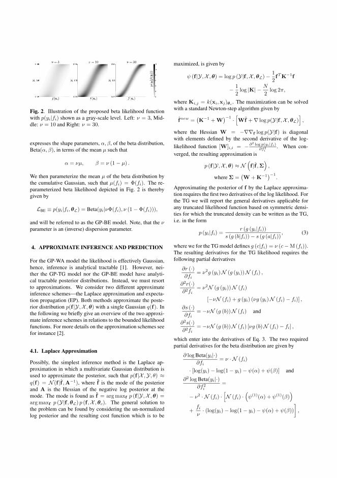
Fig. 2. Illustration of the proposed beta likelihood functionwith p(yi|fi) shown as a gray-scale level. Left: ν = 3, Mid-dle: ν = 10 and Right: ν = 30.
expresses the shape parameters, α, β, of the beta distribution,Beta(α, β), in terms of the mean µ such that
α = νµ, β = ν (1− µ) .
We then parameterize the mean µ of the beta distribution bythe cumulative Gaussian, such that µ(fi) = Φ(fi). The re-parameterized beta likelihood depicted in Fig. 2 is therebygiven by
LBE ≡ p(yi|fi,θL) = Beta(yi|νΦ(fi), ν (1− Φ(fi))),
and will be referred to as the GP-BE model. Note, that the νparameter is an (inverse) dispersion parameter.
4. APPROXIMATE INFERENCE AND PREDICTION
For the GP-WA model the likelihood is effectively Gaussian,hence, inference is analytical tractable [1]. However, nei-ther the GP-TG model nor the GP-BE model have analyti-cal tractable posterior distributions. Instead, we must resortto approximations. We consider two different approximateinference schemes—the Laplace approximation and expecta-tion propagation (EP). Both methods approximate the poste-rior distribution p(f |Y,X ,θ) with a single Gaussian q(f). Inthe following we briefly give an overview of the two approxi-mate inference schemes in relations to the bounded likelihoodfunctions. For more details on the approximation schemes seefor instance [2].
4.1. Laplace Approximation
Possibly, the simplest inference method is the Laplace ap-proximation in which a multivariate Gaussian distribution isused to approximate the posterior, such that p(f |X ,Y, θ) ≈q(f) = N (f |f ,A−1), where f is the mode of the posteriorand A is the Hessian of the negative log posterior at themode. The mode is found as f = arg maxf p (f |Y,X ,θ) =arg maxf p (Y|f ,θL) p (f ,X ,θc). The general solution tothe problem can be found by considering the un-normalizedlog posterior and the resulting cost function which is to be
maximized, is given by
ψ (f |Y,X ,θ) = log p (Y|f ,X ,θL)− 1
2fTK−1f
− 1
2log |K| − N
2log 2π,
where Ki,j = k(xi,xj)θc. The maximization can be solved
with a standard Newton-step algorithm given by
fnew =(K−1 + W
)−1 ·[Wf +∇ log p(Y|f ,X ,θL)
],
where the Hessian W = −∇∇f log p(Y|f) is diagonalwith elements defined by the second derivative of the log-likelihood function [W]i,i = −∂2 log p(yi|fi)
∂f2i
. When con-verged, the resulting approximation is
p (f |Y,X ,θ) ≈ N(f |f ,Σ
),
where Σ =(W + K−1
)−1.
Approximating the posterior of f by the Laplace approxima-tion requires the first two derivatives of the log likelihood. Forthe TG we will report the general derivatives applicable forany truncated likelihood function based on symmetric densi-ties for which the truncated density can be written as the TG,i.e. in the form
p (yi|fi) =r (g (yi|fi))
s (g (b|fi))− s (g (a|fi)), (3)
where we for the TG model defines g (c|fi) = ν (c−M (fi)).The resulting derivatives for the TG likelihood requires thefollowing partial derivatives
∂r (·)∂fi
= ν2g (yi)N (g (yi))N (fi) ,
∂2r(·)∂2fi
= ν2N (g (yi))N (fi)
[−νN (fi) + g (yi) (νg (yi)N (fi)− fi)] ,∂s (·)∂fi
= −νN (g (b))N (fi) and
∂2s(·)∂2fi
= −νN (g (b))N (fi) [νg (b)N (fi)− fi] ,
which enter into the derivatives of Eq. 3. The two requiredpartial derivatives for the beta distribution are given by
∂ log Beta(yi|·)∂fi
= ν · N (fi)
· [log(yi)− log(1− yi)− ψ(α) + ψ(β)] and
∂2 log Beta(yi|·)∂f2i
=
− ν2 · N (fi) ·[N (fi) ·
(ψ(1)(α) + ψ(1)(β)
)
+fiν· (log(yi)− log(1− yi)− ψ(α) + ψ(β))
],
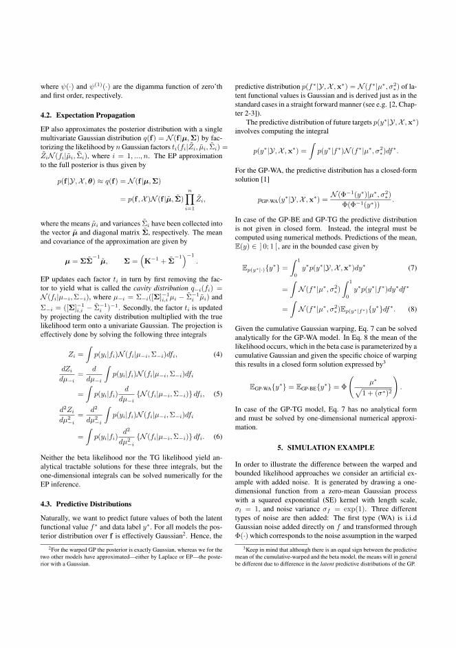
where ψ(·) and ψ(1)(·) are the digamma function of zero’thand first order, respectively.
4.2. Expectation Propagation
EP also approximates the posterior distribution with a singlemultivariate Gaussian distribution q(f) = N (f |µ,Σ) by fac-torizing the likelihood by nGaussian factors ti(fi|Zi, µi, Σi) =ZiN (fi|µi, Σi), where i = 1, ..., n. The EP approximationto the full posterior is thus given by
p(f |Y,X ,θ) ≈ q(f) = N (f |µ,Σ)
= p(f ,X )N (f |µ, Σ)n∏
i=1
Zi,
where the means µi and variances Σi have been collected intothe vector µ and diagonal matrix Σ, respectively. The meanand covariance of the approximation are given by
µ = ΣΣ−1
µ, Σ =(K−1 + Σ
−1)−1.
EP updates each factor ti in turn by first removing the fac-tor to yield what is called the cavity distribution q−i(fi) =N (fi|µ−i,Σ−i), where µ−i = Σ−i([Σ]−1i,i µi − Σ−1i µi) andΣ−i = ([Σ]−1i,i − Σ−1i )−1. Secondly, the factor ti is updatedby projecting the cavity distribution multiplied with the truelikelihood term onto a univariate Gaussian. The projection iseffectively done by solving the following three integrals
Zi =
∫p(yi|fi)N (fi|µ−i,Σ−i)dfi, (4)
dZi
dµ−i=
d
dµ−i
∫p(yi|fi)N (fi|µ−i,Σ−i)dfi
=
∫p(yi|fi)
d
dµ−i{N (fi|µ−i,Σ−i)} dfi, (5)
d2Zi
dµ2−i
=d2
dµ2−i
∫p(yi|fi)N (fi|µ−i,Σ−i)dfi
=
∫p(yi|fi)
d2
dµ2−i{N (fi|µ−i,Σ−i)} dfi. (6)
Neither the beta likelihood nor the TG likelihood yield an-alytical tractable solutions for these three integrals, but theone-dimensional integrals can be solved numerically for theEP inference.
4.3. Predictive Distributions
Naturally, we want to predict future values of both the latentfunctional value f∗ and data label y∗. For all models the pos-terior distribution over f is effectively Gaussian2. Hence, the
2For the warped GP the posterior is exactly Gaussian, whereas we for thetwo other models have approximated—either by Laplace or EP—the poste-rior with a Gaussian.
predictive distribution p(f∗|Y,X ,x∗) = N (f∗|µ∗, σ2∗) of la-
tent functional values is Gaussian and is derived just as in thestandard cases in a straight forward manner (see e.g. [2, Chap-ter 2-3]).
The predictive distribution of future targets p(y∗|Y,X ,x∗)involves computing the integral
p(y∗|Y,X ,x∗) =
∫p(y∗|f∗)N (f∗|µ∗, σ2
∗)df∗.
For the GP-WA, the predictive distribution has a closed-formsolution [1]
pGP-WA(y∗|Y,X ,x∗) =N (Φ−1(y∗)|µ∗, σ2
∗)Φ(Φ−1(y∗))
.
In case of the GP-BE and GP-TG the predictive distributionis not given in closed form. Instead, the integral must becomputed using numerical methods. Predictions of the mean,E(y) ∈ ] 0; 1 [ , are in the bounded case given by
Ep(y∗|·){y∗} =
∫ 1
0
y∗p(y∗|Y,X ,x∗)dy∗ (7)
=
∫N (f∗|µ∗, σ2
∗)∫ 1
0
y∗p(y∗|f∗)dy∗df∗
=
∫N (f∗|µ∗, σ2
∗)Ep(y∗|f∗){y∗}df∗. (8)
Given the cumulative Gaussian warping, Eq. 7 can be solvedanalytically for the GP-WA model. In Eq. 8 the mean of thelikelihood occurs, which in the beta case is parameterized by acumulative Gaussian and given the specific choice of warpingthis results in a closed form solution expressed by3
EGP-WA{y∗} = EGP-BE{y∗} = Φ
(µ∗√
1 + (σ∗)2
).
In case of the GP-TG model, Eq. 7 has no analytical formand must be solved by one-dimensional numerical approxi-mation.
5. SIMULATION EXAMPLE
In order to illustrate the difference between the warped andbounded likelihood approaches we consider an artificial ex-ample with added noise. It is generated by drawing a one-dimensional function from a zero-mean Gaussian processwith a squared exponential (SE) kernel with length scale,σl = 1, and noise variance σf = exp(1). Three differenttypes of noise are then added: The first type (WA) is i.i.dGaussian noise added directly on f and transformed throughΦ(·) which corresponds to the noise assumption in the warped
3Keep in mind that although there is an equal sign between the predictivemean of the cumulative-warped and the beta model, the means will in generalbe different due to difference in the latent predictive distributions of the GP.
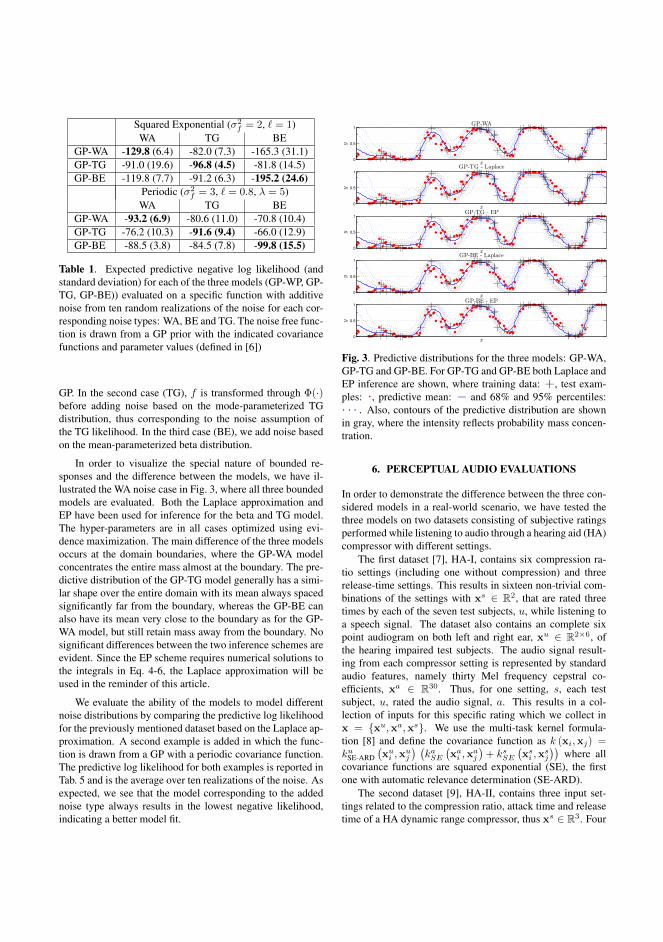
Squared Exponential (σ2f = 2, ` = 1)
WA TG BEGP-WA -129.8 (6.4) -82.0 (7.3) -165.3 (31.1)GP-TG -91.0 (19.6) -96.8 (4.5) -81.8 (14.5)GP-BE -119.8 (7.7) -91.2 (6.3) -195.2 (24.6)
Periodic (σ2f = 3, ` = 0.8, λ = 5)
WA TG BEGP-WA -93.2 (6.9) -80.6 (11.0) -70.8 (10.4)GP-TG -76.2 (10.3) -91.6 (9.4) -66.0 (12.9)GP-BE -88.5 (3.8) -84.5 (7.8) -99.8 (15.5)
Table 1. Expected predictive negative log likelihood (andstandard deviation) for each of the three models (GP-WP, GP-TG, GP-BE)) evaluated on a specific function with additivenoise from ten random realizations of the noise for each cor-responding noise types: WA, BE and TG. The noise free func-tion is drawn from a GP prior with the indicated covariancefunctions and parameter values (defined in [6])
GP. In the second case (TG), f is transformed through Φ(·)before adding noise based on the mode-parameterized TGdistribution, thus corresponding to the noise assumption ofthe TG likelihood. In the third case (BE), we add noise basedon the mean-parameterized beta distribution.
In order to visualize the special nature of bounded re-sponses and the difference between the models, we have il-lustrated the WA noise case in Fig. 3, where all three boundedmodels are evaluated. Both the Laplace approximation andEP have been used for inference for the beta and TG model.The hyper-parameters are in all cases optimized using evi-dence maximization. The main difference of the three modelsoccurs at the domain boundaries, where the GP-WA modelconcentrates the entire mass almost at the boundary. The pre-dictive distribution of the GP-TG model generally has a simi-lar shape over the entire domain with its mean always spacedsignificantly far from the boundary, whereas the GP-BE canalso have its mean very close to the boundary as for the GP-WA model, but still retain mass away from the boundary. Nosignificant differences between the two inference schemes areevident. Since the EP scheme requires numerical solutions tothe integrals in Eq. 4-6, the Laplace approximation will beused in the reminder of this article.
We evaluate the ability of the models to model differentnoise distributions by comparing the predictive log likelihoodfor the previously mentioned dataset based on the Laplace ap-proximation. A second example is added in which the func-tion is drawn from a GP with a periodic covariance function.The predictive log likelihood for both examples is reported inTab. 5 and is the average over ten realizations of the noise. Asexpected, we see that the model corresponding to the addednoise type always results in the lowest negative likelihood,indicating a better model fit.
x
y
GP-WA
0
0.5
1
x
y
GP-BE - Laplace
0
0.5
1
xy
GP-BE - EP
0
0.5
1
x
y
GP-TG - Laplace
0
0.5
1
x
y
GP-TG - EP
0
0.5
1
Fig. 3. Predictive distributions for the three models: GP-WA,GP-TG and GP-BE. For GP-TG and GP-BE both Laplace andEP inference are shown, where training data: +, test exam-ples: ·, predictive mean: − and 68% and 95% percentiles:· · · . Also, contours of the predictive distribution are shownin gray, where the intensity reflects probability mass concen-tration.
6. PERCEPTUAL AUDIO EVALUATIONS
In order to demonstrate the difference between the three con-sidered models in a real-world scenario, we have tested thethree models on two datasets consisting of subjective ratingsperformed while listening to audio through a hearing aid (HA)compressor with different settings.
The first dataset [7], HA-I, contains six compression ra-tio settings (including one without compression) and threerelease-time settings. This results in sixteen non-trivial com-binations of the settings with xs ∈ R2, that are rated threetimes by each of the seven test subjects, u, while listening toa speech signal. The dataset also contains an complete sixpoint audiogram on both left and right ear, xu ∈ R2×6, ofthe hearing impaired test subjects. The audio signal result-ing from each compressor setting is represented by standardaudio features, namely thirty Mel frequency cepstral co-efficients, xa ∈ R30. Thus, for one setting, s, each testsubject, u, rated the audio signal, a. This results in a col-lection of inputs for this specific rating which we collect inx = {xu,xa,xs}. We use the multi-task kernel formula-tion [8] and define the covariance function as k (xi,xj) =kuSE-ARD
(xui ,x
uj
) (kaSE
(xai ,x
aj
)+ ksSE
(xsi ,x
sj
))where all
covariance functions are squared exponential (SE), the firstone with automatic relevance determination (SE-ARD).
The second dataset [9], HA-II, contains three input set-tings related to the compression ratio, attack time and releasetime of a HA dynamic range compressor, thus xs ∈ R3. Four
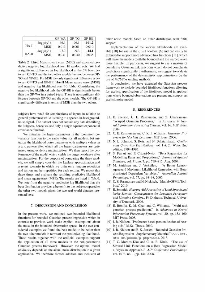
GP-WA GP-TG GP-BE
HA-I-log p(y∗) -66.1 -96.1 -101.2
MSE 0.013 0.001 0.010
HA-II-log p(y∗) -7.7 -9.3 -14.1
MSE 0.031 0.030 0.035
Table 2. HA-I Mean square error (MSE) and expected pre-dictive negative log likelihood over 10 random sets. We finda significant difference in log likelihood at the 5% level be-tween GP-TG and the two other models but not between GP-TG and GP-BE. For MSE the only significant difference is be-tween GP-TG and GP-BE. HA-II Mean square error (MSE)and negative log likelihood over 10 folds. Considering thenegative log likelihood only the GP-BE is significantly betterthan the GP-WA in a paired t-test. There is no significant dif-ference between GP-TG and the other models. The GP-BE issignificantly different in terms of MSE than the two others.
subjects have rated 50 combinations of inputs in relation togeneral preference while listening to a speech-in-background-noise signal. The dataset does not contain any data describingthe subjects, hence we use only a single squared exponentialcovariance function.
We initialize the hyper-parameters in the (common) co-variance function to the same value for all models, but ini-tialize the likelihood noise parameter with multiple values ina grid pattern after which all the hyper-parameters are opti-mized using evidence maximization. We then report the per-formance of the model which yields the largest evidence aftermaximization. For the purpose of comparing the three mod-els, we will simply consider the Laplace approximation anda retest scenario in which we train on a random repetitionand test on another repetition for each setting. We repeat thisthree times and evaluate the resulting predictive likelihoodand mean square error (MSE). The results are listed in Tab. 6.We note from the negative predictive log likelihood that thebeta distribution provides a better fit to the noise compared tothe other two models given the two real-world datasets pre-sented here.
7. DISCUSSION AND CONCLUSION
In the present work, we outlined two bounded likelihoodfunctions for bounded Gaussian process regression which incontrast to previous work make explicit assumptions aboutthe noise in the bounded observation space. In the two con-sidered examples we found the beta model to be better thanthe two other models in terms of the predictive log likelihood.These results together with the artificial examples supportthe application of all three models in the non-parametricGaussian process framework. However, the optimal modelobviously depends on the actual noise distribution in a givenapplication. We therefore foresee addition and inclusion of
other noise models based on other distribution with finitesupport.
Implementations of the various likelihoods are avail-able [10] for use in the gpml toolbox [6] and can easily beextended to support more advanced link functions [11], whichwill make the models (both the bounded and the warped) evenmore flexible. In particular, we suggest to use a mixture ofcumulative Gaussian link functions which do not complicatepredictions significantly. Furthermore, we suggest to evaluatethe performance of the deterministic approximations by theuse of MCMC-sampling methods.
In conclusion, we have extended the Gaussian processframework to include bounded likelihood functions allowingfor explicit specification of the likelihood model in applica-tions where bounded observations are present and support anexplicit noise model.
8. REFERENCES
[1] E. Snelson, C. E. Rasmussen, and Z. Ghahramani,“Warped Gaussian Processes,” in Advances in Neu-ral Information Processing Systems, vol. 16. MIT Press,2004.
[2] C. E. Rasmussen and C. K. I. Williams, Gaussian Pro-cesses for Machine Learning, MIT Press, 2006.
[3] N. L. Johnson, S. Kotz, and N. Balakrishnan, Contin-uous Univariate Distributions, vol. 1 & 2, Wiley, 2ndedition, 1994-1995.
[4] S. Ferrari and F. Cribari-Neto, “Beta Regression forModelling Rates and Proportions,” Journal of AppliedStatistics, vol. 31, no. 7, pp. 799–815, Aug. 2004.
[5] M. Smithsen and J. Verkuilen, “A Better Lemon-squeezer? Maximum Likelihood Regression with Beta-distributed Dependent Variables.,” Australian JournalPsychology, vol. 57, pp. 98–98, 2005.
[6] C. E. Rasmussen and H. Nickisch, “Matlab GPML Tool-box,” 2010.
[7] E. Schmidt, Hearing Aid Processing of Loud Speech andNoise Signals: Consequences for Loudness Perceptionand Listening Comfort., Ph.D. thesis, Technical Univer-sity of Denmark, 2006.
[8] E. Bonilla, K. M. Chai, and C. Williams, “Multi-taskgaussian process prediction,” in Advances in NeuralInformation Processing Systems, vol. 20, pp. 153–160.MIT Press, 2008.
[9] J. B. Nielsen, “Preference based personalization of hear-ing aids,” M.Sc. Thesis, 2010.
[10] J. B. Nielsen and B. S. Jensen, “Bounded Gaussian Pro-cess Regression - Supplementary Material,” www.imm.dtu.dk/pubdb/p.php?6683, 2013.
[11] T. C. Martins Dias and C. A. R. Diniz, “The use ofSeveral Link Functions on a Beta Regression Model:a Bayesian Approach.,” AIP Conference Proceedings,vol. 1073, no. 1, pp. 144, 2008.

Bibliography
[1] Last.fm dataset, the official song tags and song similarity collection for theMillion Song Dataset. http://labrosa.ee.columbia.edu/millionsong/lastfm.
[2] The Echo Nest Taste profile subset, the officialuser data collection for the Million Song Dataset.http://labrosa.ee.columbia.edu/millionsong/tasteprofile.
[3] Samer A. Abdallah, Henrik Ekeus, Peter Foster, Andrew Robertson, andMark D. Plumbley. Cognitive music modelling: An information dynamicsapproach. 2012 3rd International Workshop on Cognitive InformationProcessing, CIP 2012, page 6232940, 2012.
[4] T. S. Alstrom, Bjørn S. Jensen, Mikkel N. Schmidt, Natalie V. Kostesha,and Jan Larsen. Haussdorff and hellinger for colorimetric sensor arrayclassification. IEEE International Workshop on Machine Learning forSignal Processing, pages 1–6, 2012.
[5] M. Alvarez, L. Rosasco, and N. D. Lawrence. Kernels for Vector-ValuedFunctions: A Review. Foundations and Trends in Machine Learning,4(3):195–266, 2012.
[6] Amazon. http://amazon.com/, 2012. [Online; accessed 17-12-2012].
[7] J. Arenas-Garcıa, A. Meng, K.B. Petersen, T. Lehn-Schiøler, L.K. Hansen,and J. Larsen. Unveiling Music Structure Via pLSA Similarity Fusion,pages 419–424. IEEE, 2007.
[8] A. Asuncion, M. Welling, P. Smyth, and Y.W. Teh. On smoothing andinference for topic models. 25th Conference on Uncertainty in ArtificialIntelligence, pages 27–34, 2009.

182 BIBLIOGRAPHY
[9] J. J. Aucouturier and F. Pachet. Music similarity measures: What’s theuse? In Proceedings of 3rd International Conference on Music InformationRetrieval, pages 157–163, Paris, France, 2002.
[10] R. Baeza-Yates and B. Ribeiro-Neto. Modern Information Retrieval.Addison-Wesley, 1999.
[11] L. Barrington, A. B. Chan, and G. Lanckriet. Dynamic texture mod-els of music. International Conference on Acoustics, Speech, and SignalProcessing, pages 1589–1592, 2009.
[12] L. Barrington, A.B. Chan, and G. Lanckriet. Modeling Music as a Dy-namic Texture. IEEE Transactions on Audio, Speech, and Language Pro-cessing, 18(3):602–612, March 2010.
[13] L. Barrington, D. Turnbull, and G. Lanckriet. Game-powered machinelearning. Proceedings of the National Academy of Sciences of the UnitedStates of America, 109(17):6411–6, April 2012.
[14] L. Barrington and M. Yazdani. Combining feature kernels for semanticmusic retrieval. International Conference on Music Information Retrieval,2008.
[15] M. A. Bartsch and G. H. Wakefield. To catch a chorus: Using chroma-based representations for audio thumbnailing. In IEEE Workshop on Ap-plications of Signal Processing to Audio and Acoustics (WASPAA), NewPaltz, NY, October 2001.
[16] S. Bech and N. Zacharov. Perceptual Audio Evaluation - Theory, Methodand Application. Cambridge University Press, 2006.
[17] S. Beggs, S. Cardell, and J. Hausman. Assessing the potential demand forelectric cars. Journal of Econometrics, 17(1):1, 1981.
[18] T Bertin-Mahieux. Clustering beat-chroma patterns in a large musicdatabase. In International Society for Music Information Retrieval Con-ference, 2010.
[19] T. Bertin-Mahieux, D. Eck, F. Maillet, and P. Lamere. Autotagger: AModel for Predicting Social Tags from Acoustic Features on Large MusicDatabases. Journal of New Music Research, 37(2):115–135, June 2008.
[20] T. Bertin-Mahieux, D. P.W. Ellis, B. Whitman, and P. Lamere. Themillion song dataset. In Proceedings of the 12th International Conferenceon Music Information Retrieval (ISMIR 2011), 2011.
[21] W. Bialek, I. Nemenman, and N. Tishby. Predictability, complexity, andlearning. Neural Computation, 13(11):2409–2463, 2001.

BIBLIOGRAPHY 183
[22] A. Birlutiu, P. Groot, and T. Heskes. Multi-task preference learningwith an application to hearing aid personalization. Neurocomputing, 73(7-9):1177–1185, March 2010.
[23] A. Birlutiu, P Groot, and T. Heskes. Multi-task preference learning withan application to hearing aid personalization. Neurocomputing, 73(7-9):1177–1185, March 2010.
[24] A. Birlutiu, P. Groot, and T. Heskes. Efficiently learning the preferencesof people. Machine Learning, pages 1–28, 2012.
[25] C.M. Bishop. Neural networks for pattern recognition. Clarendon Press,1995.
[26] C.M. Bishop. Pattern Recognition and Machine Learning. Springer, 2006.
[27] D. Blei and J. Lafferty. Correlated Topic Models. In Y Weiss, B Scholkopf,and J Platt, editors, Advances in Neural Information Processing Systems18, pages 147–154. MIT Press, Cambridge, MA, 2006.
[28] D. Blei and J. McAuliffe. Supervised topic models. In J.C. Platt, D. Koller,Y. Singer, and S. Roweis, editors, Advances in Neural Information Pro-cessing Systems 20, pages 121–128. MIT Press, Cambridge, MA, 2008.
[29] D. M Blei, A. Ng, and M. Jordan. Latent dirichlet allocation. The Journalof Machine Learning Research, 3:993–1022, 2003.
[30] R.D. Bock and J.V. Jones. The measurement and prediction of judgmentand choice. 1968.
[31] E. Bonilla, S. Guo, and S. Sanner. Gaussian Process Preference Elicitation.In J Lafferty, C K I Williams, J Shawe-Taylor, R S Zemel, and A Culotta,editors, Advances in Neural Information Processing Systems 23, pages262–270. 2010.
[32] E.. V. Bonilla, F. V. Agakov, and C. K.I. Williams. Kernel multi-tasklearning using task-specific features. Journal of Machine Learning Re-search, 2:43–50, 2007.
[33] Voice Box. http://www.ee.ic.ac.uk/hp/staff/dmb/voicebox/
voicebox.html, 2012. [Online; accessed 17-12-2012].
[34] R.A. Bradley. Rank analysis of incomplete block designs .2. additionaltables for the method of paired comparisons. Biometrika, 41(3-4):502–537, 1954.
[35] R.A. Bradley and M.E. Terry. Rank analysis of incomplete block designs.1. the method of paired comparisons. Biometrika, 39(3-4):324–345, 1952.
184 BIBLIOGRAPHY
[36] P.B. Brockhoff and R.H.B. Christensen. Thurstonian models for sensorydiscrimination tests as generalized linear models. Food Quality and Pref-erence, 21(3):330–338, 2010.
[37] Chris Burges, Tal Shaked, Erin Renshaw, Ari Lazier, Matt Deeds, NicoleHamilton, and Greg Hullender. Learning to rank using gradient descent.ACM International Conference Proceeding Series, 119:89–96, 2005.
[38] Auditory Toolbox by M. Slaney. https://engineering.purdue.edu/
~malcolm/interval/1998-010/, 2012. [Online; accessed 17-12-2012].
[39] CAL-500. http://cosmal.ucsd.edu/cal/, 2012. [Online; accessed 17-12-2012].
[40] Zhe Cao, Tao Qin, Tie-Yan Liu, Hang Li, and Ming-Feng Tsai. Learningto rank: From pairwise approach to listwise approach. ACM InternationalConference Proceeding Series, 227:129–136, 2007.
[41] G. Casella. An Introduction to Empirical Bayes Data Analysis. TheAmerican Statistician, 39(2):83–87, 1985.
[42] O. Celma. Foafing the music bridging the semantic gap in music rec-ommendation. In 5th International Semantic Web Conference (ISWC),Athens, GA, USA, 2006.
[43] O. Celma. Music Recommendation and Discovery in the Long Tail.Springer, New Work, 2010.
[44] Kathryn Chaloner and Isabella Verdinelli. Bayesian experimental design:A review. Statistical Science, 10:273–304, 1995.
[45] Gang Chen, Tian-Jiang Wang, and Perfecto Herrera. A novel mu-sic retrieval system with relevance feedback. 3rd International Confer-ence on Innovative Computing Information and Control, ICICIC’08, page4603347, 2008.
[46] W. Chu and Z Ghahramani. Extensions of Gaussian processes for ranking:semi-supervised and active learning. In Workshop Learning to Rank atAdvances in Neural Information Processing Systems 18, 2005.
[47] W. Chu and Z. Ghahramani. Gaussian processes for ordinal regression.Journal of Machine Learning Research, 6, 2005.
[48] W. Chu and Z. Ghahramani. Preference learning with Gaussian pro-cesses. ICML 2005 - Proceedings of the 22nd International Conference onMachine Learning, pages 137–144, 2005.

BIBLIOGRAPHY 185
[49] D. A. Cohn, Z. Ghahramani, and M.I.. Jordan. Active learning withstatistical models. Journal of Artificial Intelligence Research, 4:129–145,1996.
[50] T.M. Cover and J.A. T. Elements of information theory. Wiley, 1991.
[51] A. M Croom. Music, neuroscience, and the psychology of well-being: aprecis. Frontiers in psychology., 2:393, 2012.
[52] I. Cross. Cognitive science and the cultural nature of music. Topics inCognitive Science, 4(4):668, 2012.
[53] L. Csato. Gaussian Processes - Iterative Sparse Approximations. PhDthesis, Aston University, 2002.
[54] CSIRAC. http://news.bbc.co.uk/2/hi/technology/7458479.stm,2008. [Online; accessed 17-12-2012].
[55] S. Deerwester, S. T. Dumais, G. W. Furnas, T. K. Landauer, and R. Harsh-man. Indexing by latent semantic analysis. Journal of the American So-ciety for Information Science, 41(6):391–407, 1990.
[56] J. R. Deller and J. H. L. Hansen. Discrete-Time Processing of SpeechSignals. Prentice Hall, New Jersey, 1987.
[57] D. Deutsch. The psychology of music. Academic Press, 1999. AcademicPress Series in Cognition and Perception.
[58] C. Ding, T. Li, and W. Peng. On the equivalence between non-negativematrix factorization and probabilistic latent semantic indexing. Compu-tational Statistics and Data Analysis, 52(8):3913–3927, 2008.
[59] D. K. Duvenaud, H. Nickisch, and C.E. Rasmussen. Additive gaussianprocesses. In J. Shawe-Taylor, R.S. Zemel, P. Bartlett, F.C.N. Pereira,and K.Q. Weinberger, editors, Advances in Neural Information ProcessingSystems 24, pages 226–234. 2011.
[60] The Echonest. http://the.echonest.com/, 2012. [Online; accessed 17-12-2012].
[61] D. Ellis. In International Conference on Music Information Retrieval (IS-MIR).
[62] D. P. W. Ellis and B. Whitman. The quest for ground truth in musicalartist similarity. SIGCHI International Symposium on Music InformationRetrieval, 2002.
[63] A Faisal, J Gillberg, J Peltonen, G Leen, and S Kaski. Sparse Nonpara-metric Topic Model for Transfer Learning. dice.ucl.ac.be.
186 BIBLIOGRAPHY
[64] R.M. Fano. Transmission of Information. M.I.T. Press, first edition, 1961.
[65] V. V. Fedorov. Theory of optimal experiments. Academic Press, 1972.
[66] S. Ferrari and F. Cribari-Neto. Beta Regression for Modelling Rates andProportions. Journal of Applied Statistics, 31(7):799–815, August 2004.
[67] Gaussian Process for Machine Learning (GPML toolbox). http://www.
gaussianprocess.org/gpml/code/matlab/doc/, 2012. [Online; accessed17-12-2012].
[68] J. Frow. Genre. Routledge, New York, NY, USA, 2005.
[69] T. Fujishima. Realtime chord recognition of musical sound: A systemusing common lisp music. International Computer Music Conference(ICMC), pages 465–467, 1999.
[70] Y. Gao, I. Kontoyiannis, and E. Bienenstock. Estimating the entropyof binary time series: Methodology, some theory and a simulation study.Entropy, 10(2):71–99, 2008.
[71] R. Garnett, M. A. Osborne, and S. J. Roberts. Bayesian optimization forsensor set selection. Information Processing In Sensor Networks, pages209–219, 2010.
[72] G Geleijnse, M. Schedl, and P Knees. The quest for ground truth inmusical artist tagging in the social web era. International Conference onMusic Information Retrieval, 2007.
[73] A. Gelman. Prior distributions for variance parameters in hierarchicalmodels. Bayesian Analysis, 1(3):515–533, 2006.
[74] M. Girolami and S. Rogers. Variational bayesian multinomial probit re-gression with gaussian process priors. Neural Computation, 18(8):1790–1817, 2006.
[75] M. E. Glickman and Shane T. Jensen. Adaptive paired comparison design.Journal of Statistical Planning and Inference, 127(1-2):279–293, 2005.
[76] B. Gold and N. Morgan. Speech and Audio Signal Processing / Processingand Perception of Speech and Music. John Wiley and sons Inc., 2000.
[77] F. Gouyon and S. Dixon. A review of automatic rhythm description sys-tems. Computer Music Journal, 29(1):34–54, 2005.
[78] T. L Griffiths and M. Steyvers. Finding scientific topics. Proceedings ofthe National Academy of Sciences of the United States of America, 101Suppl:5228–35, April 2004.
BIBLIOGRAPHY 187
[79] P Groot, A. Birlutiu, and T. Heskes. Bayesian Monte Carlo for the globaloptimization of expensive functions. Proc. of ECAI, 1(1.5):2, 2010.
[80] J. Guiver and E. Snelson. Bayesian inference for plackett-luce rankingmodels. Proceedings of the 26th International Conference On MachineLearning, ICML 2009, pages 377–384, 2009.
[81] B. Haasdonk and C. Bahlmann. Learning with distance substitution ker-nels. In in Pattern Recognition, Proceedings of the 26th DAGM Sympo-sium, 2004.
[82] P. Hamel and D. Eck. Learning features from music audio with deepbelief networks. In Proceedings of the 11th International Society for MusicInformation Retrieval Conference (ISMIR), pages 339–344, August 2010.
[83] L.K. Hansen, P. Ahrendt, and J. Larsen. Towards cognitive componentanalysis. In AKRR 2005-International and Interdisciplinary Conferenceon Adaptive Knowledge Representation and Reasoning, 2005.
[84] V.L. Hansen. Functional analysis - entering Hilbert space. World Scientific,2006.
[85] J. S. Hare, P. A. S. Sinclair, P. H. Lewis, K. Martinez, P. Enser, and C. J.Sandom. Bridging the semantic gap in multimedia information retrieval:Top-down and bottom-up approaches. In Mastering the Gap: From Infor-mation Extraction to Semantic Representation / 3rd European SemanticWeb Conference, 2006.
[86] R. Henao and O. Winther. Pass-gp: Predictive active set selection forgaussian processes. IEEE International Workshop on Machine Learningfor Signal Processing 2010 (MLSP 2010), pages 148–153, 2010.
[87] H. Hermansky. Perceptual linear predictive plp analysis of speech. Journalof the Acoustical Society of America, 87(4):1738–1752, 1990.
[88] K Hevner. Experimental studies of the elements of expression in music.American Journal of Psychology, 48:246–268, 1936.
[89] K. M. Higgins. Biology and culture in musical emotions. Emotion Review(SAGE Journals), 4(3):273–282, 2012.
[90] M. Hoffman, D. Blei, and P Cook. Content-based musical similarity com-putation using the hierarchical dirichlet process. In 9th International Con-ference on Music Information Retrieval, pages 349–354, 2008.
[91] M Hoffman, D Blei, and P Cook. Easy as CBA: A simple probabilisticmodel for tagging music. International Society for Music InformationRetrieval Conference, pages 369–374, 2009.

188 BIBLIOGRAPHY
[92] T. Hofmann. Probabilistic latent semantic analysis. Proceedings of Un-certainty in Artificial Intelligence, pages 289–296, 1999.
[93] N. Houlsby, Jose Miguel Hernandez-Lobato, Ferenc Huszar, andZ. Ghahramani. Collaborative gaussian processes for preference learn-ing. In P. Bartlett, F.C.N. Pereira, C.J.C. Burges, L. Bottou, and K.Q.Weinberger, editors, Advances in Neural Information Processing Systems25, pages 2105–2113. 2012.
[94] X. Hu and S. Downie. When lyrics outperform audio for music moodclassification: A feature analysis. In 11th International Society for MusicInformation Retrieval Conference, pages 619–624, 2010.
[95] Digital Music Report 2012 IFPI. http://http://www.ifpi.org/
content/library/DMR2012.pdf/, 2012. [Online; accessed 23-12-2012].
[96] Santner T. J., Brian J Williams, and William Notz. The Design andAnalysis of Computer Experiments. Springer Series in Statistics, 2003.
[97] T. Jebara and A. Howard. Probability Product Kernels. Journal of Ma-chine Learning Research, 5:819–844, 2004.
[98] J. H. Jensen, D. P. W. Ellis, M G. Christensen, and S Holdt Jensen. Eval-uation of distance measures between gaussian mixture models of mfccs.8th International Conference on Music Information Retrieval, 2007.
[99] N. Jiang, P. Grosche, V. Konz, and M. Muller. Analyzing chroma fea-ture types for automated chord recognition. In 42nd AES Conference onSemantic Audio, Ilmenau, Germany, 2011.
[100] T. Joachims. Optimizing search engines using clickthrough data. In-ternational Conference on Knowledge Discovery and Data Mining, pages133–142, 2002.
[101] D. R Jones. A Taxonomy of Global Optimization Methods Based onResponse Surfaces. Journal of Global Optimization, 21(4):345–383, 2001.
[102] D. R Jones, M. Schonlau, and William J Welch. Efficient Global Optimiza-tion of Expensive Black-Box Functions. Journal of Global Optimization,13(4):455–492, 1998.
[103] P. N. Juslin. Are musical emotions invariant across cultures? EMOTIONREVIEW, 4(3):283–284, 2012.
[104] P. N. Juslin and P. Laukka. Expression, Perception, and Induction ofMusical Emotions: A Review and a Questionnaire Study of EverydayListening. Journal of New Music Research, 33(3):217–238, September2004.

BIBLIOGRAPHY 189
[105] S K., S Narayanan, and S Sundaram. Acoustic topic model for audio in-formation retrieval. IEEE Workshop on Applications of Signal Processingto Audio and Acoustics, pages 37–40, 2009.
[106] Sofia K-Means. http://code.google.com/p/sofia-ml/wiki/
SofiaKMeans, 2012. [Online; accessed 21-12-2012].
[107] Y.E. Kim, E. Schmidt, and L. Emelle. Moodswings: A collaborativegame for music mood label collection. International Conference on MusicInformation Retrieval, pages 231–236, 2008.
[108] Y.E. Kim, E.M. Schmidt, Raymond Migneco, B.G. Morton, PatrickRichardson, Jeffrey Scott, J.A. Speck, and Douglas Turnbull. Music emo-tion recognition: A state of the art review. In 11th International MusicInformation Retrieval Conference, pages 255–266, 2010.
[109] A. Klapuri and M. Davy. Signal processing methods for music transcrip-tion. Springer, 2006. Includes bibliographical references (p. [391]-428) andindex.
[110] P. Knees and G. Widmer. Searching for music using natural languagequeries and relevance feedback. Advances in Neural Information Process-ing Systems, 4918:109–121, 2008.
[111] I. Kontoyiannis, P.H. Algoet, Yu M. Suhov, and A.J. Wyner. Nonpara-metric entropy estimation for stationary process and random fields, withapplications to english text. IEEE Transactions on Information Theory,44(3):1319–1327, 1998.
[112] M. W. Krasilovsky, Sidney Shemel, John M. Gross, and Jonathan Fein-stein. This Business of Music, 10th Edition. Billboard Books, 2007.
[113] A. Krause and C. Guestrin. Nonmyopic active learning of Gaussian pro-cesses: An exploration- exploitation approach. 24th International Confer-ence on Machine Learning, pages 449–456, 2007.
[114] A. Krithara, M. Amini, C. Goutte, and J. Renders. An extension of theaspect plsa model to active and semi-supervised learning for text classi-fication. ARTIFICIAL INTELLIGENCE: THEORIES, MODELS ANDAPPLICATIONS, PROCEEDINGS, 6040:183–192, 2010.
[115] A. Krithara, C. Goutte, M.-R. Amini, and J.-M. Renders. Reducing theannotation burden in text classification. International Conference on Mul-tidisciplinary Information Sciences and Technologies, 2(1):279–283, 2006.
[116] H.J. Kushner. New method of locating maximum point of arbitrary mul-tipeak curve in presence of noise. Joint Automatic Control Conference,pages 69–79, 1963.
190 BIBLIOGRAPHY
[117] S. Lacoste-Julien, Fei Sha, and M. Jordan. DiscLDA: DiscriminativeLearning for Dimensionality Reduction and Classification. In D Koller,D Schuurmans, Y Bengio, and L Bottou, editors, Advances in Neural In-formation Processing Systems 21, pages 897–904. 2009.
[118] P. Lamere. Social tagging and music information retrieval. Journal ofNew Music Research, 37(2):101–114, 2008.
[119] last.fm. http://last.fm/, 2012. [Online; accessed 17-12-2012].
[120] E. Law and L. Von Ahn. Input-agreement: A new mechanism for collectingdata using human computation games. In ACM SIGCHI Conference onHuman Factors in Computing Systems. ACM Press, 2009.
[121] N. Lawrence, M. Seeger, and R. Herbrich. Fast sparse gaussian processmethods: The informative vector machine. Advances in Neural Informa-tion Processing Systems, (15):625–632, 2003.
[122] M. Lazaro-Gredilla. Bayesian warped gaussian processes. In P. Bartlett,F.C.N. Pereira, C.J.C. Burges, L. Bottou, and K.Q. Weinberger, editors,Advances in Neural Information Processing Systems 25, pages 1628–1636.2012.
[123] D.D. Lee and H.S. Seung. Learning the parts of objects by non-negativematrix factorization. Nature, 401(6755):788–791, 1999.
[124] H. Lee, L. Yan, P. Pham, and A. Y. Ng. Unsupervised feature learning foraudio classification using convolutional deep belief networks. Advancesin Neural Information Processing Systems 22 - Proceedings of the 2009Conference, pages 1096–1104, 2009.
[125] M. Levy and M. Sandler. Learning Latent Semantic Models for Musicfrom Social Tags. Journal of New Music Research, 37(2):137–150, June2008.
[126] M. Levy and M. Sandler. Music information retrieval using social tagsand audio. IEEE Transactions on Multimedia, 11(3):383–395, 2009.
[127] M. S. Lew, N. Sebe, C. Djeraba, and R. Jain. Content-based multime-dia information retrieval. ACM Transactions on Multimedia Computing,Communications, and Applications, 2(1):1–19, February 2006.
[128] R. Likert. A technique for the measurement of attitudes. Archives ofPsychology, 22(140):1–55, 1932.
[129] D V Lindley. On a Measure of the Information Provided by an Experiment.The Annals of Mathematical Statistics, (4):986–1005, 1956.

BIBLIOGRAPHY 191
[130] D. V. Lindley. Bayesian statistics. a review. Regional Conference Seriesin Applied Mathematics, (2):1–83, 1971.
[131] D.V. LINDLEY. On a measure of the information provided by an exper-iment. Annals of Mathematical Statistics, 27(4):986–1005, 1956.
[132] Daniel Lizotte, Tao Wang, Michael Bowling, Dale Schuurmansdepartment,and Computing Science. Gaussian process regression for optimization.2008.
[133] B. Logan. Mel Frequency Cepstral Coefficients for Music Modeling. In InInternational Symposium on Music Information Retrieval, 2000.
[134] B. Logan and A. Salomon. A music similarity function based on signalanalysis. Multimedia and Expo, 2001, IEEE International Conference on,2001.
[135] R.D. Luce. Individual Choice Behavior: A Theoretical Analysis. Wiley(New York), 1959.
[136] D. MacKay. The evidence framework applied to classification networks.Neural Computation, 4(5):720–736, 1992.
[137] D. MacKay. The evidence framework applied to classification networks.Neural Computation, 4(5):720–736, 1992.
[138] D.J.C. MacKay. Information-based objective functions for active dataselection. Neural Computation, 4(4):590–604, 1992.
[139] D.J.C. MacKay. Introduction to Gaussian processes. NATO ASI SeriesF Computer and Systems Sciences, 168:133–166, 1998.
[140] J. Madsen. Modeling of Emotions expressed in Mu-sic using Audio features. DTU Informatics, MasterThesis, http://www2.imm.dtu.dk/pubdb/views/publicationdetails.php?id=6036, 2011.
[141] C. L. Mallows. Non-null ranking models i. Biometrika, 44(1/2):114–130,1957.
[142] M. Mandel and D. Ellis. A Web-Based Game for Collecting Music Meta-data. Journal of New Music Research, 37(2):151–165, June 2008.
[143] M. I. Mandel and Daniel P. W. Ellis. Song-Level Features and Sup-port Vector Machines for Music Classification. In Joshua D. Reiss andGeraint A. Wiggins, editors, Proceedings of the 6th International Confer-ence on Music Information Retrieval (ISMIR), pages 594–599, September2005.

192 BIBLIOGRAPHY
[144] C. D. Manning, P Raghavan, and H. Schutze. Introduction to informationretrieval. Cambridge University Press, 2008.
[145] P. McCullagh and J.A. Nelder. Generalized linear models. Chapman andHall, 1989. Monographs on statistics and applied probability : 37.
[146] B. McFee, L. Barrington, and G. Lanckriet. Learning content similarityfor music recommendation. IEEE Transactions on Audio, Speech, andLanguage Processing, 20(8):2207–2218, 2012.
[147] B McFee and G. Lanckriet. Metric learning to rank. International Con-ference on Machine Learning, 2010.
[148] B. McFee and G. R. G. Lanckriet. Hypergraph models of playlist dialects.In Proceedings of the 13th International Society for Music InformationRetrieval Conference, pages 343–348, 2012.
[149] Matt Mcvicar and Tijl De Bie. CCA and a multi-way extension for inves-tigating common components between audio , lyrics and tags. In CMMR,number June, pages 19–22, 2012.
[150] A. Meng. Temporal Feature Integration for Music Organisation. PhDthesis, Technical University of Denmark, DTU, 2006.
[151] A. Meng, P. Ahrendt, and J. Larsen. Improving music genre classificationby short-time feature integration. IEEE International Confonference onAcoustics Speech Signal Processing, 5:497–500, 2004.
[152] A. Meng and J. Shawe-Taylor. An investigation of feature models formusic genre classification using the support vector classifier. InternationalConference on Music Information Retrieval, pages 604–609, 2005.
[153] P. Mermelstein. Distance Measures for Speech Recognition–Psychologicaland Instrumental. In Joint Workshop on Pattern Recognition and Artifi-cial Intelligence, 1976.
[154] T. Minka. A family of algorithms for approximate Bayesian inference.PhD thesis, MIT, 2001.
[155] R. Miotto, L. Barrington, and G. Lanckriet. Improving Auto-taggingby Modeling Semantic Co-occurrences. In International Society of MusicInformation Retrieval Conference, pages 297–302, 2010.
[156] J. Mockus, V. Tiesis, and Zilinskas A. The application of Bayesian meth-ods for seeking the extremum. Towards Global Optimization, 2:117–129,1978.
[157] L.L. Mølgaard. Context based multimedia information retrieval. PhDthesis, Technical Univeristy of Denmark, 2008.

BIBLIOGRAPHY 193
[158] D. C. Montgomery. Design and analysis of experiments. Wiley, 2009.
[159] B. C. J. Moore. An Introduction to the Psychology of Hearing, FifthEdition. Academic Press, April 2003.
[160] M.. Muller. Information retrieval for music and motion. Springer, 2009.
[161] M. Muller, D. P. W. Ellis, A. Klapuri, and G. Richard. Signal processingfor music analysis. IEEE Journal of Selected Topics in Signal Processing,5(6):1088–1110, 2011.
[162] I. Murray and R.P. Adams. Slice sampling covariance hyperparameters oflatent Gaussian models. arXiv preprint arXiv:1006.0868, 2(1):1–9, 2010.
[163] T. Næ s, P.B. Brockhoff, and O. Tomic. Statistics for sensory and con-sumer science. Wiley, 2010.
[164] A Naish-Guzman. The generalized FITC approximation. Advances inNeural Information Processing Systems, pages 1–8, 2008.
[165] R.M. Neal. Monte Carlo implementation of Gaussian process models forBayesian regression and classification. Technical report, 1997.
[166] Netflix. http://netflix.com/, 2012. [Online; accessed 17-12-2012].
[167] H. Nickisch and C.E. Rasmussen. Approximations for binary gaussian pro-cess classification. JOURNAL OF MACHINE LEARNING RESEARCH,9(1):2035–2078, 2009.
[168] H. Nickisch and M. Seeger. Multiple Kernel Learning: A Unifying Prob-abilistic Viewpoint. arXiv preprint arXiv:1103.0897, 2011.
[169] A. B. Nielsen, L. K. Hansen, and U. Kjems. Pitch based sound classifica-tion. ICASSP, IEEE International Conference on Acoustics, Speech andSignal Processing - Proceedings, 3:III788–III791, 2006.
[170] Jens Brehm Nielsen and J. Nielsen. Efficient individualization of hearingaid processes sound. Submittet to the IEEE International Conference onSpeech Audio and Signal Processing (ICASSP 2013), 2013.
[171] Nielsen.com. http://www.nielsen.com/us/en/insights/press-room/
2012/music-discovery-still-dominated-by-radio--says-nielsen-music-360.
html, 2012. [Online; accessed 23-12-2012].
[172] M. Osborne. Bayesian Gaussian Processes for Sequential Prediction ,Optimisation and Quadrature. PhD thesis, University of Oxford, 2010.
[173] R. P. Paiva. Melody detection in polyphonic audio. PhD thesis, 2006.
194 BIBLIOGRAPHY
[174] E. Pampalk, T. Pohle, and G. Widmer. Dynamic playlist generation basedon skipping behavior. In Proceedings of 6th International Conference onMusic Information Retrieval, London, UK, 2005.
[175] Y. Panagakis, C. Kotropoulos, and G.R. Arce. Music genre classifica-tion using locality preserving nonnegative tensor factorization and sparserepresentations. 2011.
[176] G. Peeters. A large set of audio features for sound description (similarityand classification) in the CUIDADO project. Techical report, IRCAM,2004.
[177] M. K. Petersen, M. Mørup, and L. K. Hansen. Sparse but emotionaldecomposition of lyrics. In 3rd International Workshop on Learning Se-mantics of Audio Signals (LSAS), pages 31–43, 2009.
[178] R.L. Plackett. The analysis of permutations. Applied Statistics, 24(2):193–202, 1975.
[179] J. Quinonero Candela and C.E. Rasmussen. A unifying view of sparse ap-proximate Gaussian process regression. The Journal of Machine LearningResearch, 6:1939–1959, 2005.
[180] L.R. Rabiner. A tutorial on hidden markov models and selected applica-tions in speech recognition. 2009.
[181] F. Rahman and J. Siddiqi. Semantic annotation of digital music. J.Comput. Syst. Sci., 78(4):1219–1231, July 2012.
[182] C.E. Rasmussen and C. K I Williams. Gaussian Processes for MachineLearning. MIT Press, 2006.
[183] J. Robinson. The expression and arousal of emotion in music. Journal ofAesthetics and Art Criticism, 1994.
[184] J.A. Russel. A circumplex model of affect. Journal of Personality andSocial Psychology, 39(6):1161–1178, 1980.
[185] O. Sacks. Musicophilia: Tales of Music and the Brain. Knopf DoubledayPublishing Group, 2007.
[186] J. Salamon and E. Gomez. Melody extraction from polyphonic musicsignals using pitch contour characteristics. IEEE Transactions on Audio,Speech, and Language Processing, 20(6):1759–1770, 2012.
[187] P. Sandhaus and S. Boll. Semantic analysis and retrieval in personal andsocial photo collections. Multimedia Tools and Applications, 51(1):5–33,December 2010.

BIBLIOGRAPHY 195
[188] M. Schedl and Peter Knees. Personalization in Multimodal Music Re-trieval. 9th International Workshop on Adaptive Multimedia Retrieval,2011.
[189] A Schindler, R Mayer, and A Rauber. Facilitating comprehensive bench-marking experiments on the million song dataset. In 13th InternationalConference on Music Information Retrieval (ISMIR 2012). 2012.
[190] G. Schwarz. Estimating the dimension of a model. The Annals of Statis-tics, 6(2):461–464, 1978.
[191] M. Seeger, C. K. I. Williams, N. D. Lawrence, and Sheeld S Dp. Fastforward selection to speed up sparse gaussian process regression. In inWorkshop on AI and Statistics 9, 2003.
[192] M. W. Seeger, N. D. Lawrence, and R. Herbrich. Efficient nonparametricbayesian modelling with sparse gaussian process approximations. Tech-nical report, Max Planck Institute for Biological Cybernetics, Tubingen,Germany, 2006.
[193] W. A. Sethares. Tuning, timbre, spectrum, scale. Springer, 2nd ed. edition,2005. Includes bibliographical references (p. [381]-397) and index.
[194] B. Settles. Active learning. Synthesis Lectures on Artificial Intelligenceand Machine Learning, 18:1–111, 2012.
[195] H S Seung, M Opper, and H Sompolinsky. Query by committee. Pro-ceedings of the Fifth Annual ACM Workshop on Computational LearningTheory, pages 287–294, 1992.
[196] K Seyerlehner, G Widmer, and P Knees. Frame level audio similarity - acodebook approach. Conference on Digital Audio Effects, pages 1–8, 2008.
[197] J. Shawe-Taylor and Nello Cristianini. Kernel methods for pattern analy-sis. Cambridge University Press, 2004.
[198] A. W. M. Smeulders, M. Worring, S. Santini, A. Gupta, and R. Jain.Content-based image retrieval at the end of the early years. IEEE Trans-actions on Pattern Analysis and Machine Intelligence, 22(12):1349–1380,2000.
[199] E. Snelson and Z. Ghahramani. Sparse Gaussian Processes using Pseudo-Inputs. Advances in neural information processing, 2006.
[200] E. Snelson, Z. Ghahramani, and Rasmussen C.E. Warped gaussian pro-cesses. Advances in Neural Information Processing Systems, (16):337–344,2004.

196 BIBLIOGRAPHY
[201] C. Song, Z. Qu, N. Blumm, and Albert-Laszlo Barabasi. Limits of pre-dictability in human mobility. Science, 327(5968):1018–1021, 2010.
[202] C. Song, Z. Qu, N. Blumm, and Albert-Laszlo Barabasi. Limits of pre-dictability in human mobility - supplementary material, 2010.
[203] M. Sordo, Oscar Celma, Martin Blech, and Enric Guaus. The quest formusical genres: Do the experts and the wisdom of crowds agree? In 9thInternational Conference on Music Information Retrieval, pages 255–260,2008.
[204] M. Sordo, F. Gouyon, L. Sarmento, and O. Celma. Inferring semanticfacets of a music folksonomy with wikipedia. Journal of Web Semantics,Submitted.
[205] N. Srinivas, A. Krause, S. M. Kakade, and M. Seeger. Information-theoretic regret bounds for gaussian process optimization in the bandit set-ting. IEEE Transactions on Information Theory, 58(5):3250–3265, 2012.
[206] S. Stober and N A. Towards User-Adaptive Structuring and Organizationof Music Collections. pages 53–65, 2010.
[207] S. Stober and A. Nurnberger. An experimental comparison of similarityadaptation approaches. In International Society for Music InformationRetrieval Conference, 2011.
[208] S. Stober and A. Nurnberger. Adaptive music retrieval - a state of theart. Multimedia Tools and Applications, March 2012.
[209] B.L. Sturm. A survey of evaluation in music genre recognition. AdaptiveMultimedia Retrieval, 2012.
[210] S. Sundaram and S. Narayanan. Audio retrieval by latent perceptualindexing. International Conference on Acoustics, Speech and Signal Pro-cessing, pages 49–52, 2008.
[211] R. S. Taylor. The process of asking questions. American Documentation,13(4):391–396, October 1962.
[212] Y.W. Teh, M.I. Jordan, M.J. Beal, and D.M. Blei. Hierarchical dirichletprocesses. Journal of the American Statistical Association, 101, 2004.
[213] H. Terasawa, M. Slaney, and J. Berger. A timbre space for speech. InINTERSPEECH 2005 - Eurospeech, 9th European Conference on SpeechCommunication and Technology, Lisbon, Portugal, September 4-8, 2005,pages 1729–1732. ISCA, 2005.
[214] William R. Thompson. On the theory of apportionment. American Jour-nal of Mathematics, 57(2):450–456, 1935.
BIBLIOGRAPHY 197
[215] W.R. Thompson. On the likelihood that one unknown probability exceedsanother in view of the evidence of two samples. Biometrika, 25:285–294,1933.
[216] L L Thurstone. A law of comparative judgement. Psychological Review,34, 1927.
[217] M.E. Tipping. Sparse Bayesian learning and the relevance vector machine.The Journal of Machine Learning Research, 2001.
[218] S. Tong and D. Koller. Support vector machine active learning with ap-plications to text classification. Journal of Machine Learning Research,2(1):45–66, 2002.
[219] Intelligent Sound Processing Toolbox. http://kom.aau.dk/project/
isound/, 2012. [Online; accessed 17-12-2012].
[220] K. Train. Discrete Choice Methods with Simulation. Cambridge UniversityPress, 2009.
[221] D. Turnbull, Ruoran Liu, Luke Barrington, and G. Lanckriet. A game-based approach for collecting semantic annotations of music. ISMIR, 2008.
[222] J. Vanhatalo. Speeding up the inference in Gaussian process models. PhDthesis, Alto University, 2010.
[223] J. Vanhatalo, P. Jylanki, and A. Vehtari. Gaussian process regressionwith Student-t likelihood. In Y Bengio, D Schuurmans, J Lafferty, C K IW.s, and A Culotta, editors, Advances in Neural Information ProcessingSystems 22, pages 1910–1918. 2009.
[224] A. Vehtari and J. Ojanen. A survey of bayesian predictive methods formodel assessment, selection and comparison. Statistics Surveys, 6:142,2012.
[225] J. V. Verkuilen. Regression Models for Paired Comparisons. PhD thesis,University of Illinois at Urbana-Champaign, 2007.
[226] C. Walder, Kwang K., and B. Scholkopf. Sparse multiscale gaussian pro-cess regression. International Conference on Machine Learning, pages1112–1119, 2008.
[227] H. M. Wallach, I. Murray, Ruslan Salakhutdinov, and D. Mimno. Evalu-ation methods for topic models. Proceedings of the 26th Annual Interna-tional Conference on Machine Learning - ICML ’09, (d):1–8, 2009.
[228] Hanna M. Wallach. Structured topic models for language. PhD thesis,University of Cambridge, 2008.
198 BIBLIOGRAPHY
[229] J Weston, S Bengio, and P Hamel. Multi-Tasking with Joint SemanticSpaces for Large- Scale Music Annotation and Retrieval Multi-Taskingwith Joint Semantic Spaces for Large-Scale Music Annotation and Re-trieval. Journal of New Music Research, (November 2012):37–41, 2011.
[230] T.D. Wickens. Elementary signal detection theory. Oxford UniversityPress, Inc., 2002.
[231] C.I. Williams and D. Barber. Bayesian classification with Gaussian pro-cesses. IEEE Transactions on Pattern Analysis and Machine Intelligence,20(12):1342–1351, 1998.
[232] A. Wilson and Z. Ghahramani. Copula Processes. Advances in NeuralInformation Processing Systems 23, pages 2460–2468, 2010.
[233] Ole Winther. Bayesian Mean Field Algorithms for Neural Networks andGaussian Processes. PhD thesis, 1998.
[234] D. Wolff and T Weyde. Adapting similarity on the MagnaTagATunedatabase: effects of model and feature choices. International World WideWeb Conference, 2012.
[235] D Wolff, T Weyde, S. Stober, and A Nurnberger. A systematic comparisonof music similarity adaptation approaches. 13th International Society forMusic Information Retrieval Conference, pages 103–108, 2012.
[236] F. Xia, J. Wang, W. Zhang, T. Liu, and H. Li. Listwise approach tolearning to rank - theory and algorithm. ICML 2008 - Proceedings of the25th International Conference on Machine Learning, pages 1192–1199,2008.
[237] Yi-Hsuan Yang and Homer H Chen. Ranking-based emotion recognitionfor music organization and retrieval. IEEE Transactions on Audio, Speech,and Language Processing, 19(4):762–774, 2011.
[238] G. Yao and U. Bockenholt. Bayesian destimation of thurstonian rankingmodels based on the gibbs sampler. British Journal of Mathematical andStatistical Psychology, 52(1):79, 1999.
[239] K. Yoshii and M Goto. Continuous pLSI and smoothing techniques for hy-brid music recommendation. International Society for Music InformationRetrieval Conference, pages 339–344, 2009.
[240] K. Yoshii, M Goto, and K Komatani. Hybrid collaborative and content-based music recommendation using probabilistic model with latent userpreferences. International Society for Music Information Retrieval Con-ference, 2006.

BIBLIOGRAPHY 199
[241] Y. Yue, T. Finley, F. Radlinski, and T. Joachims. A support vector methodfor optimizing average precision. Proceedings of the international ACMSIGIR conference on Research and development in Information Retrieval,pages 271–278, 2007.
[242] J. Zhu and T. Hastie. Kernel logistic regression and the import vectormachine, 2001.
[243] E. Zwicker and H. Fastl. Psychoacoustics: Facts and models. SpringerSeries in Information Sciences, 22(2), 1999.