Combining Bottom-Up and Top-Down

Christoph Bohringer

Department of Economics, University of Oldenburg

Centre for European Economic Research (ZEW), Mannheim

boehringer@uni-oldenburg.de

Thomas F. Rutherford

Ann Arbor, Michigan

tom@mpsge.org

Revised March, 2007

Abstract

We motivate the formulation of market equilibrium as a mixed complementarity problem which

explicitly represents weak inequalities and complementarity between decision variables and equi-

librium conditions. The complementarity format permits an energy-economy model to combine

technological detail of a bottom-up energy system with a second-best characterization of the over-

all economy. Our primary objective is pedagogic. We first lay out the complementarity features

of economic equilibrium and demonstrate how we can integrate bottom-up activity analysis into a

top-down representation of the broader economy. We then provide a stylized numerical example of

an integrated model – within both static and dynamic settings. Finally, we present illustrative ap-

plications to three themes figuring prominently on the energy policy agenda of many industrialized

countries: nuclear phase-out, green quotas, and environmental tax reforms.

JEL classification: C61, C68, D58, Q43

Keywords: Computable General Equilibrium, Complementarity, Bottom-Up, Top-Down

1 Introduction

There are two wide-spread modeling approaches for the quantitative assessment of economic impacts

induced by energy policies: bottom-up models of the energy system and top-down models of the

1

broader economy. The two model classes differ mainly with respect to the emphasis placed on

technological details of the energy system vis-a-vis the comprehensiveness of endogenous market

adjustments.

Bottom-up energy system models are partial equilibrium representations of the energy sector.

They feature a large number of discrete energy technologies to capture substitution of energy

carriers on the primary and final energy level, process substitution, or efficiency improvements.

Such models often neglect the macroeconomic impact of energy policies. Bottom-up energy system

models are typically cast as optimization problems which compute the least-cost combination of

energy system activities to meet a given demand for final energy or energy services subject to

technical restrictions and energy policy constraints.

Top-down models adopt an economy-wide perspective taking into account initial market distor-

tions, pecuniary spillovers, and income effects for various economic agents such as households or

government. Endogeneity in economic responses to policy shocks typically comes at the expense of

specific sectoral or technological details. Conventional top-down models of energy-economy inter-

actions have a limited representation of the energy system. Energy transformation processes are

characterized by smooth production functions which capture local substitution (transformation)

possibilities through constant elasticities of substitution (transformation). As a consequence, top-

down models usually lack detail on current and future technological options which may be relevant

for an appropriate assessment of energy policy proposals. In addition, top-down models may not

assure fundamental physical restrictions such as the conservation of matter and energy.

The specific strengths and weaknesses of the bottom-up and top-down approaches explain the

wide range of hybrid modeling efforts that combine technological explicitness of bottom-up models

with the economic comprehensiveness of top-down models (see Hourcade, Jaccard, Bataille and

Gershi (2006)). These efforts may be distinguished into three broader categories: First, indepen-

dently developed bottom-up and top-down models can be linked. This approach has been adopted

since the early 1970’s, but it often challenges overall coherence due to inconsistencies in behavioral

assumptions and accounting concepts across “soft-linked” models.1 Second, one could focus on

one model type – either bottom-up or top-down – and use “reduced form” representations of the

other. Prominent examples include ETA-Macro (Manne (1977)) and its successor MERGE (Manne,

Mendelsohn and Richels (2006)) which link a bottom-up energy system model with a highly aggre-

gate one-sector macro-economic model of production and consumption within a single optimization

framework. Recent hybrid modelling approaches based on the same technique are described in

Bahn, Kypreos, Bueler and Luethi (1999), Messner and Schrattenholzer (2000), or Bosetti, Car-

raro, Galeotti, Massetti and Tavoni (2006). The third approach provides completely integrated

models based on developments of solution algorithms for mixed complementarity problems during

1See e.g. Hofman and Jorgenson (1976), Hogan and Weyant (1982), Messner and Strubegger (1987), Drouet, Haurie,Labriet, Thalmann, Vielle and Viguier (2005), or Schafer and Jacoby (2006)

2

the 1990’s (Dirkse and Ferris (1995), Rutherford (1995)). In an earlier paper, Bohringer (1998)

stresses the difference between bottom-up and top-down with respect to the characterization of

technology options and associated input substitution possibilities in production. More lately, Schu-

macher and Sands (2006) investigate process shifts and changes in the fuel input structure for

the steel industry comparing an aggregate top-down production characterisation with a bottom-up

description of technologies for producing iron and steel. Both papers highlight the importance

of “true” technology-based activity analysis in evaluating policy-induced structural change at the

sectoral level.

In this paper, we focus on the third approach to hybrid modeling, i.e. the direct combination

of bottom-up and top-down in a complementarity format. Our primary objective is pedagogic.

We show that complementarity is a feature of economic equilibrium rather than an equilibrium

condition per se. Complementarity can then be exploited to cast an economic equilibrium as a

mixed complementarity problem. The complementarity format facilitates weak inequalities and

logical connections between prices and market conditions. These properties permit the modeler

to integrate bottom-up activity analysis directly within a top-down representation of the broader

economy. Apart from accommodating technological explicitness in an economy-wide framework,

the mixed complementarity approach relaxes so-called integrability conditions that are inherent

to economic models formulated as optimization problem (see Pressman (1970) or Takayma and

Judge (1971)). First-order conditions from primal or dual mathematical programs impose efficient

allocation which rules out common second-best phenomena. Since many policy issues are associated

with second-best characteristics of the real world – such as initial tax distortions or market failures

– the optimization approach to integrate bottom-up and top-down is limited in the scope of policy

applications. Non-integrabilities furthermore reflect empirical evidence that individual demand

functions depend not only on prices but also on factor incomes. In such cases, demand functions

are typically not integrable into an economy-wide utility function (see e.g.Rutherford (1999b)) and

income effects matter (Hurwicz (1999) or Russell (1999)).2

Given the coherence and comprehensiveness of the complementarity format, we want to demon-

strate how this approach can be implemented for applied energy policy analysis. In section 2, we

provide a formal exposition of the complementarity features of economic equilibria and illustrate

the direct integration of bottom-up energy system activity analysis into top-down economic mod-

eling. In section 3, we develop a stylized numerical example of a hybrid bottom-up /top-down

model – within both static and dynamic settings. In section 4, we illustrate application of this type

of model by considering three prominent themes on the energy policy agenda of many industrial-

ized countries: nuclear phase-out, green quotas, and environmental tax reforms. In section 5, we

conclude. Our paper documents algebraic structure and data inputs to the simulations reported

2Only if the matrix of cross-price elasticities, i.e. the first-order partial derivatives of the demand functions, issymmetric, is there an associated optimization problem which can be used to compute the equilibrium prices andquantities.

3

herein. The interested reader can download the computer programs to replicate our results from

http://www.mpsge.org/td-bu.zip. 3

2 Complementarity and Arrow-Debreu Equilibria

We consider a competitive economy with n commodities (including primary factors), m production

activities (sectors), and h households. The decision variables of the economy can be classified into

three categories (Mathiesen (1985)):

p is a non-negative n-vector (with running index i) in prices for all goods and

factors,

y denotes a non-negative m-vector (with running index j) for activity levels of

constant-returns-to-scale (CRTS) production sectors, and

M represents a non-negative k-vector (with running index h) in incomes.

A competitive market equilibrium is characterized by a vector of activity levels (y ≥ 0), a vector

of prices (p ≥ 0 ), and a vector of incomes (M) such that:

• Zero profit implies that no production activity makes a positive profit, i.e.:

−Πj(p) ≥ 0 (1)

where:

Πj(p) denotes the unit-profit function for CRTS production activity j, which is cal-

culated as the difference between unit revenue and unit cost.4

• Market clearance requires that supply minus demand is non-negative for all goods and factors,

i.e.: ∑j

yj∂Πj(p)

∂pi+

∑h

wih ≥∑

h

dih(p,Mh) ∀i (2)

where:

wih indicates the initial endowment matrix by commodity andhousehold),∂Πj(p)

∂piis (by Hotelling’s lemma) the compensated supply of good i per unit operation

of activity j, and

dih(p,Mh) is the utility maximizing demand for good i by household h.

3We have implemented our models using GAMS/MCP (see Brooke, Kendrick and Meeraus (1996) and Rutherford(1995)) as well as GAMS/MPSGE (Rutherford 1999a) using the PATH solver (Dirkse and Ferris 1995).

4Technologies are assumed to exhibit constant returns to scale, hence the unit-profit function is homogeneous of

degree one in prices, and by Euler’s theorem Πj =∑

i pi∂Πj(p)

∂pi.

4

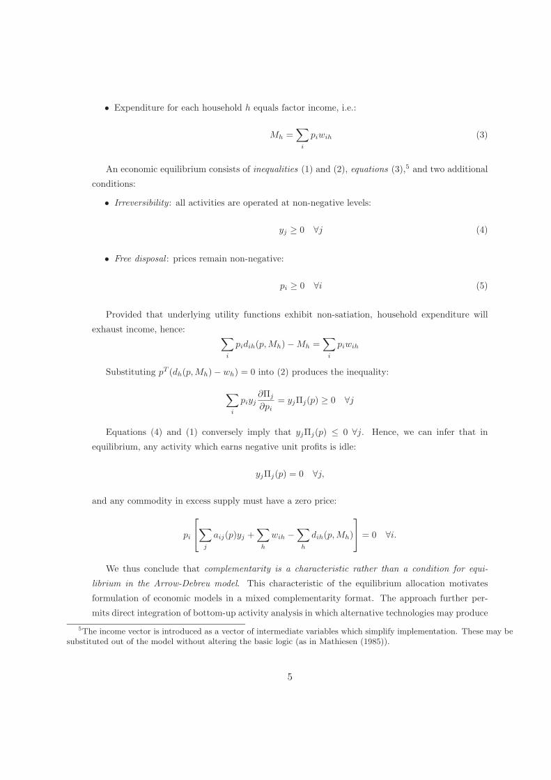
• Expenditure for each household h equals factor income, i.e.:

Mh =∑

i

piwih (3)

An economic equilibrium consists of inequalities (1) and (2), equations (3),5 and two additional

conditions:

• Irreversibility : all activities are operated at non-negative levels:

yj ≥ 0 ∀j (4)

• Free disposal : prices remain non-negative:

pi ≥ 0 ∀i (5)

Provided that underlying utility functions exhibit non-satiation, household expenditure will

exhaust income, hence: ∑i

pidih(p,Mh) − Mh =∑

i

piwih

Substituting pT (dh(p,Mh) − wh) = 0 into (2) produces the inequality:

∑i

piyj∂Πj

∂pi= yjΠj(p) ≥ 0 ∀j

Equations (4) and (1) conversely imply that yjΠj(p) ≤ 0 ∀j. Hence, we can infer that in

equilibrium, any activity which earns negative unit profits is idle:

yjΠj(p) = 0 ∀j,

and any commodity in excess supply must have a zero price:

pi

⎡⎣∑

j

aij(p)yj +∑

h

wih −∑

h

dih(p,Mh)

⎤⎦ = 0 ∀i.

We thus conclude that complementarity is a characteristic rather than a condition for equi-

librium in the Arrow-Debreu model. This characteristic of the equilibrium allocation motivates

formulation of economic models in a mixed complementarity format. The approach further per-

mits direct integration of bottom-up activity analysis in which alternative technologies may produce

5The income vector is introduced as a vector of intermediate variables which simplify implementation. These may besubstituted out of the model without altering the basic logic (as in Mathiesen (1985)).

5

one or more products subject to process-oriented capacity constraints. As a canonical example,

we may consider the energy sector linear programming problem which seeks to find the least-cost

schedule for meeting an exogenous set of energy demands using a given set of energy technologies,

t:

min∑

t

ctyt (6)

subject to

∑t

ajtyt = dj ∀j ∈ {energy goods}

∑t

bktyt ≤ κk ∀k ∈ {energy resources}

yt ≥ 0

where:

yt is the activity level of energy technology t,

ajt denotes the netput of energy good j by technology t (energy goods may be

either inputs or outputs),

ct is the exogenous marginal cost of technology t,

dj represents market demand for energy good j,

bkt represents the unit demand for energy resource k by technology t, and

κk is the aggregate supply of energy resource, k. Such resources may include

generation, pipeline or transmission capacities, some of which may be specific

to an individual technology and others which may be traded in markets and

thus transferred to most efficient use.We write bars over ct and dj indicating that while these parameters are taken as given from the

standpoint of firms in the energy sector, their values are determined as part of the outer economic

equilibrium model.

When we derive the Kuhn-Tucker conditions characterize optimality of this linear program, we

obtain: ∑t

ajtyt = dj , πj ≥ 0, πj

(∑t

ajtyt = dj

)= 0 (7)

and ∑t

bityt ≤ κi, μi ≥ 0, μi

(∑t

bityt ≤ κi

)= 0, (8)

where:

6

πj is the Lagrange multiplier on the price-demand balance for energy good j, and

μi is the shadow price on the energy sector resource i.

Comparing the Kuhn-Tucker conditions with our market equilibrium model, we note an equiv-

alence between the shadow prices of mathematical programming constraints and market prices.

The mathematical program can be interpreted as a special case of the general equilibrium problem

where (i) income constraints are dropped, (ii) energy demands are exogenous, and (iii) energy sup-

ply technologies are characterized by fixed as opposed to price-responsive coefficients. In turn, we

can replace an aggregate top-down description of energy good production in the general equilib-

rium setting by the Kuhn-Tucker conditions of the linear program, thereby providing technological

details while treating all prices as endogenous.

The weak duality theorem relates the optimal value of the linear program to shadow prices and

constants appearing in the constraint equations:

∑j

πjdj =∑

t

ctyt +∑

k

μkκk (9)

Equation (9) provides one further insight into the relationship of the bottom-up linear program-

ming model and the outer economic environment. It represents a zero-profit condition (see equation

(1)), applied to the aggregate energy subsector: in equilibrium, the value of produced energy goods

and services equals the market value of resource rents and variable costs of energy production.

Beyond the direct integration of bottom-up activity analysis, the complementarity represen-

tation readily accomodates income effects and important second-best characteristics such as tax

distortions or market failures (externalities). The latter are typically incoporated through explicit

bounds on decisions variables such as prices or activity levels. Examples of price constraints may

include lower bounds on the real wage or prescribed price caps (upper bounds) on energy goods.

As to quantity constraints, examples may include administered bounds on the share of specific

energy sources (e.g. renewables or nuclear power) or target levels for the provision of public goods.

Associated with these constraints are complementary variables. In the case of price constraints, a

rationing variable applies as soon as the price constraint becomes binding; in the case of quantity

constraints, a complementary endogenous subsidy or tax is introduced.

3 A Maquette

As a pedagogic introduction to the ideas introduced in the previous section, we now provide a

concrete example of the integration of bottom-up technological details into a top-down general

equilibrium framework. We consider a stylized representation of the world economy with basic

7

economic transactions displayed in Table 1.6

After describing a static setting without investment activities we subsequently lay out an in-

tertemporal extension of the static model where agents make explicit choices at the margin between

current and future consumption based on consistent expectations of future prices.

To maintain transparency and simplicity in this exposition, we formulate a model involving a

single macroeconomic good and a representative consumer. Extensions of the model to deal with

multiple non-energy goods and multiple households are, in our view, relatively straightforward.

3.1 A Static Model

We consider a model in with a single non-energy good produced under constant returns to scale

using inputs of labor, capital, and energy. The economy is closed. Three fossil fuels (oil, coal

and natural gas) are produced subject to decreasing returns to scale. Final consumption demand

includes non-energy goods, electricity, and non-electric energy. To maintain clarity, we initially

consider an economy in the absence of taxes or public goods provision.

Following the structure of the Arrow-Debreu model presented above, we denote decision vari-

ables in the model as follows:

• Activity levels:

Y is the production of non-energy good,

Xf refers to the supply of fossil-fuel f ∈ {oil, coal, gas},Et denotes the production of electricity by technology t,

C refers to composite final consumption, and

W is the full consumption (utility) including leisure.

• Market prices:

pY is the price of non-energy output,

pC is the price of the final consumption composite,

pele denotes the electricity price,

pf denotes the price of fossil fuel f ,

pL refers to the price of labor,

rK is the rental price of capital,

pW is the utility price index,

μt is the shadow price on generating capacity, and

rf is the rental rate on fossil fuel resources (f ∈ {oil, coal, gas}).• Income levels:

M portrays income of the representative household.

6The numbers stem from the GTAP 6 database which reports consistent accounts of national production and con-sumption as well as bilateral trade and energy flows for the year 2001 (Dimaranan and Dougall (2006)).

8

On the production side, firms minimize costs of producing output subject to nested constant-

elasticity-of-substitution (CES) functions that describe the price-dependent use of factors and inter-

mediate inputs. In the production of non-energy output, fossil fuels trade off in the lowest nest with

a constant elasticity of substitution. At the next level, the fossil fuel composite is combined with

electricity at constant value shares (Cobb-Douglas). The energy aggregate and a Cobb-Douglas

value-added composite enter the top level with a constant elasticity of substitution. The unit-profit

function of macro-good production is:

ΠY = pY −⎧⎨⎩θKL(pθL

L r1−θL

K )1−σY + (1 − θKL) ∗ (pθELE

ELE (∑

f

θYf p1−σE

f )1−θELE1−σE )1−σY

⎫⎬⎭

11−σY

(10)

where:

θKL is the cost share of the value-added composite in production,

θL denotes the labor cost share within the value-added composite in production,

θELE represents the electricity value share within the aggregate energy demand of

production,

θYf is the cost share of fossil fuel f within the non-electric energy composite of

production,

σY is the elasticity of substitution between the value-added composite and aggre-

gate energy in production,

σE is the elasticity of substitution between electricity and the non-electric energy

composite in production, and

Y is the associated complementary variable.

Fossil fuels are produced with a fuel-specific resource and a non-resource composite trading off

with a constant elasticity of substitution. The unit-profit function for fossil fuel production is:

ΠFf = pf −

⎧⎨⎩θR

f r1−σf

f + (1 − θRf )(θL

f pL + θKf rK + θY

f pY + θELEf pELE +

∑ff

θfffpff )1−σf

⎫⎬⎭

11−σf

(11)

where:

9

θRf denotes the cost share of resources,

θLf is the labor cost share in the non-resource composite input,

θKf refers to the capital cost share in the non-resource composite input,

θYf is the macro-good cost share in the non-resource composite input,

θELEf denotes the electricity cost share in the non-resource composite input,

θfff refers to the cost share of fossil fuel ff (aliased with f) in the non-resource

composite input,

σf is the elasticity of substitution between the fossil fuel resource and the com-

posite of non-resource inputs, and

Xf is the associated complementary variable.

In our stylized example, we illustrate the integration of bottom-up activity analysis into the

top-down representation of the overall economy through our portrayals of the electricity sector.

Rather than describing electricity generation by means of a CES production function, we capture

production possibilities by Leontief technologies that are active or inactive in equilibrium depending

on their profitability. The detailed technological representation can be necessary for an appropriate

assessment of selected policies. For example, energy policies may prescribe target shares of specific

technologies in overall electricity production such as green quotas or the gradual elimination of

certain power generation technologies such as a nuclear phase-out. We can write the unit-profit

functions of power generation technologies as:

ΠEt = pele − aY

t p − aKt rK − aL

t pL −∑

f

aFftpf − μt (12)

where:

aYt denotes the macro-good input coefficient for technology t

aKt is the capital input coefficient,

aLt refers to the labor input coefficient,

aFft is the energy input coefficient (e.g. coal, oil, or gas inputs), and

Et is the associated complementary variable.

Final consumption demand is characterized by a composite good with a three-level nested CES

technology. Fossil fuels enter in the third level (non-electric) energy nest at a unitary elasticity of

substitution. The non-electric energy composite is combined at the second level with electricity

subject to a constant elasticity of substitution. At the top level the energy aggregate trades off with

non-energy macro-good demand at a constant elasticity of substitution. The unit-profit function

10

for final consumption is written:

ΠC = pC −

⎧⎪⎨⎪⎩θCp1−σC

Y + (1 − θC)

⎡⎣θC

ELEp1−σC

ELE

ele + (1 − θCELE)(

∏f

pθC

f

f )1−σCELE

⎤⎦

1−σC1−σC

ELE

⎫⎪⎬⎪⎭

1(1−σC )

(13)

where:

θC represents the non-energy share of expenditure,

θCELE refers to the electricity value share of energy demand in final consumption,

θCf is the value share of fossil fuel f within the non-electric energy demand of final

consumption,

σC is the compensated elasticity of substitution between energy and non-energy in

final demand,

σCELE is the compensated elasticity of substitution between electric and non-electric

energy in final demand, and

C is the associated complementary variable.

Final consumption demand is combined with leisure at a constant elasticity of substitution to

form an aggregate utility good. The unit-profit function for aggregate utility is written:

ΠW = pW − {θW p1−σW

L + (1 − θW )p1−σW

C

} 11−σW (14)

where:

θW represents the leisure value share of aggregate utility,

σW is the compensated elasticity of substitution between leisure and the final con-

sumption composite, and

W is the associated complementary variable.

In our stylized economy, a representative household is endowed with primary factors labor (more

generally: time), capital, and resources for fossil fuel production. The representative household

maximizes utility from consumption subject to available income. Total income of the household

consists of factor payments and scarcity rents on capacity constraints:

M = pLZ + rKK +∑

f

rfRt +∑

t

μtEt (15)

where:Z denotes the aggregate endowment with time,

K represents the aggregate capital endowment,

Rf refers to the resource endowment with fossil fuel f , and

Et denotes the generation capacity for technology t.

11

Flexible prices on competitive markets for factors and goods assure balance of supply and

demand. Using Hotelling’s lemma, we can derive compensated supply and demand functions of

goods and factors.

Market clearance conditions for our stylized economy then read as:

• Labor market clearance:

Z − ∂ΠW

∂pLW ≥ ∂ΠY

∂pLY +

∑f

∂ΠF

∂pLxf +

∑t

aLt Et (16)

where pL is the associated complementary variable.

• Capital market clearance:

K ≥ ∂ΠY

∂rKY +

∑f

∂ΠF

∂rKxf +

∑t

aKt Et (17)

where rK is the associated complementary variable.

• Market clearance for fossil fuel resources:

Rf ≥ ∂ΠFf

∂rfXf (18)

where rf is the associated complementary variable.

• Market clearance for electricity generation capacities:

Et ≥ Et (19)

where μt is the associated complementary variable.

• Market clearance for the non-energy macro good:

Y ≥∑

f

∂ΠF

∂pYxf +

∑t

aYt Et +

∂ΠC

∂pYC (20)

where pY is the associated complementary variable.

• Market clearance for fossil fuels

Xf ≥ ∂ΠY

∂pfY +

∑ff �=f

∂ΠF

∂pffxff +

∑t

aFftEt +

∂ΠC

∂pfC (21)

where pf is the associated complementary variable.

12

• Market clearance for electricity:

∑t

Xt ≥ ∂ΠY

∂pELEY +

∑f

∂ΠF

∂pELExf +

∂ΠC

∂pELEC (22)

where pELE is the associated complementary variable.

• Market clearance for the final consumption composite:

C ≥ ∂ΠW

∂pC(23)

where pC is the associated complementary variable.

• Market clearance for the aggregate utility good:

W ≥ M

pW(24)

where pW is the associated complementary variable.

As to the parameterization of our simple numerical model, benchmark prices and quantities,

together with exogenous elasticities determine the free parameters of the functional forms that

describe technologies and preferences.

Table 1 describes the benchmark equilibrium in terms of a social accounting matrix (King

(1985)). In a microconsistent social accounting matrix data, consistency requires that the sums of

entries across each of the rows and columns equal zero: Market equilibrium conditions are associated

with the rows, the columns capture the zero-profit condition for production sectors as well as the

income balance for the aggregate household sector. Benchmark data are typically reported as

values, i.e. they are products of prices and quantities. In order to obtain separate price and

quantity observations, the common procedure is to choose units for goods and factors so that they

have a price of unity (net of potential taxes or subsidies) in the benchmark equilibrium. Then, the

value terms simply correspond to the physical quantities.7 Table 2 provides a summary of elasticities

of substitution underlying our central case simulations. Table 3 lists the initial endowments of the

economy with time, capital, and fossil fuel resources. Table 4 provides a bottom-up description

of initially active power technologies (here: gas-fired power plants, coal-fired power plants, nuclear

power plants, and hydro power plants) for the base year. Note that the benchmark outputs of

active technologies sum up to economy-wide electricity demand while input requirements add up

to aggregate demands as reported in the social accounting matrix. In our exposition, we impose

consistency of aggregate top-down data with bottom-up technology data. In modelling practise, the

harmonization of bottom-up data with top-down data may require substantial data adjustments

7Of course, one could adopt relative prices different from one and rescale physical quantities accordingly withoutaffecting the equilibrium properties.

13

to create a consistent database for the hybrid model. Table 5 includes bottom-up technology

coefficients (cost data) for initially inactive technologies (here: wind, solar, and biomass). In

our central case simulations, unit-output of inactive wind, biomass, and solar technologies are

characterized by a technology-specific cost disadvantage vis--vis the electricity price in the base

year: wind is listed as 10% more costly, biomass as 30% and solar as 100%. We furthermore

assume hydro power and nuclear power plants to operate at upper capacity levels (initially with

zero shadow prices) due to natural resource and exogenous policy constraints.

3.2 A Dynamic Extension of the Model

Policy interference can substantially affect investment and savings incentives. Assessment of the

adjustment path and long-term equilibrium effects induced by policy constraints may therefore call

for an explicit intertemporal framework.

Dynamic modeling requires an assumption on the degree of foresight of economic agents. In a

deterministic setting, one logically consistent approach is to assume that agents in the model know

as much about the future as the modeler: Agents’ expectations of future prices then correspond

to realized future prices in the simulation. Within the standard Ramsey model of savings and

investment, the notion of perfect foresight is coupled with the assumption of an infinitely-lived

representative agent who makes explicit choices at the margin between the consumption levels of

current and future generations. The representative agent maximizes welfare subject to an intertem-

poral budget constraint. Savings rates equalize the marginal return on investment and the marginal

cost of capital formation. Rates of return are determined such that the marginal productivity of a

unit of investment and marginal utility of foregone consumption are equalized.

Casting our static model into an intertemporal version only requires a few modifications, since

most of the underlying economic relationships are strictly intra-period and, therefore, hold on a

period-by-period basis in the dynamic extension. Regarding capital stock formation and investment,

an efficient allocation of capital, i.e. investment over time, implies two central intertemporal zero-

profit conditions which relate the cost of a unit of investment, the return to capital, and the purchase

price of a unit of capital stock in period τ .

Firstly, in equilibrium, the market value of a unit of depreciated capital purchased at the

beginning of period t can be no less than the value of capital rental services through that period

and the value of the unit of capital sold at the start of the subsequent period (zero-profit condition

of capital formation):

−ΠKτ = pK

τ − rKτ − (1 − δ)pK

τ+1 ≥ 0. (25)

Secondly, the opportunity to undertake investments in year τ limits the market price of capital in

period τ + 1 (zero-profit condition of investment):

−ΠIτ = −pK

τ+1 + pYτ ≥ 0 (26)

14

Furthermore, capital evolves through geometric investment and geometric depreciation:

Ki,τ+1 = (1 − δ)Ki,τ + Ii,τ (27)

Finally, output markets in the dynamic model must account for intermediate demand, final

consumption demand and investment demand:

Y ≥∑

f

∂ΠF

∂pYxf +

∑t

aYt Et +

∂ΠC

∂pYC + Iτ (28)

The foregoing equations have introduced δ, the capital depreciation rate, and three additional

variables: pKτ is the value (purchase price) of one unit of capital stock in period τ ,

Kτ is the associated dual variable which indicates the activity level of capital stock

formation in period τ , and

Iτ is the associated dual variable which indicates the activity level of aggregate

investment in period τ .

In our intertemporal model demand responses arise from behavioral choices consistent with

maximization of a infinitely-lived representative agent. This consumer allocates lifetime income,

i.e., the intertemporal budget, over time in order to maximize utility, solving:

max∑

τ

(1

1 + ρ

)τ

u(Cτ ) (29)

subject to

∑τ

pCτ Cτ = M

where:

u(.) denotes the instantaneous utility function of the representative agent, and

ρ is the time preference rate, and

M represents lifetime income (from endowments with capital, time, and resources).

With isoelastic lifetime utility the instantaneous utility function is given as:

u(c) =c1− 1

η

1 − 1η

(30)

where η is a constant intertemporal elasticity of substitution.

The finite model horizon poses some problems with respect to capital accumulation. Without

any terminal constraint, the capital stock at the end of the model’s horizon would have no value

and this would have significant repercussions for investment rates in the periods leading up to

the end of the model horizon. In order to correct for this effect, we define a terminal constraint

15

which forces investment to increase in proportion to final consumption demand. Since the model is

formulated as a mixed complementarity problem one can include the post-terminal capital stock as

an endogenous variable. Using state variable targeting for this variable, the growth of investment

in the terminal period can be related to the growth rate of capital or any other “stable” quantity

variable in the model (Lau, Pahlke and Rutherford (2002)).

For the calibration of the dynamic model we adopt central case values of 5 % for the time

preference rate (i.e. the baseline interest rate), 2 % for the growth rate of labor in efficiency units,

and 7 % for the depreciation rate of capital. These parameter values then are used to infer the

value of payments to capital across sectors and the gross value of capital formation in consistency

with a balanced steady-state growth path. The value for the constant intertemporal elasticity of

substitution η is set at 0.5.

4 Policy Simulations

In this section, we illustrate the use of our stylized hybrid bottom-up/top-down model for the

economic assessment of three initiatives that figure prominently on the energy policy agenda of

many industrialized countries: (i) nuclear phase-out, (ii) target quotas for renewables in electricity

production (green quotas), and (iii) environmental tax reforms.

For each policy initiative, we first report impacts for the static model and then present the

effects for the dynamic model.8 The dynamic model covers a time horizon of roughly a 100 years

(starting in 2005 and ending in 2100) at annual steps. In accordance with the static model setting,

we first compute an off-the-steady-state baseline accounting for resource limits on renewables (here:

hydro power is limited to the base-year level) and policy constraints on nuclear power (nuclearcan

not exceed the base-year level). The implications of policy interference are measured against the

respective baseline path (the business-as-usual BaU ) and reported in decadal periods.

An important caveat applies: Reflecting our primary pedagogic objective, both the policy sce-

narios as well as the model formulations are highly stylized such that we caution against too literal

an interpretation of the numerical results.

4.1 Nuclear Phase-Out

Reservations against the use of nuclear power are reflected in policy initiatives of several EU Member

States (e.g. Belgium, Germany, the Netherlands, Spain, and Sweden) that foresee a gradual phase-

out of their nuclear power programs (IEA (2001)). In our hybrid model, policy constraints on the

use of nuclear power can be easily implemented via parametric changes of upper bounds on the

permissible generation capacity.

8Our results section is restrained to the central case parameterization. The interested reader can alter the parame-terization in the computer programs of the download to perform sensitivity analysis.

16

Figure 1 reports static welfare changes – measured in terms of Hicksian equivalent variation

in income – as a function of upper bounds to nuclear power generation. Welfare impacts are

depicted for two alternative assumptions regarding technological backup options. The case labeled

as “Fossil” does not restrict the use of fossil power technologies whereas the case labeled as “No

fossil” restricts fossil-fuel based power generation to the initial (base-year) level. Obviously, the

welfare cost of a nuclear phase-out are much higher as we impose additional restrictions on the

phase-in of competitive power generation based on fossil fuels (for example due to climate policy

considerations). In the case “Fossil”, nuclear power is backed up by an increase in fossil power

generation whereas renewable technologies – apart from hydro which is already operated at the

upper bound in the reference situation – remain slack activities. If we forbid expansion of fossil

power generation, wind power takes up the role of the primary nuclear backup given our illustrative

cost parameterization of technologies. For the later case (i.e. “No Fossil”), Figure 2 illustrates the

changes in the supply of electricity across technologies as a function of upper bounds to nuclear

power generation.

In the dynamic model setting, we investigate a linear phase-out of nuclear power between

2010 and 2030. Figure 3 depicts the implications for investment, consumption, and aggregate

electricity supply through time. During the phase-out period, investment and electricity supply

are distinctly supressed, recovering to some extent in the long run, however at levels below the

baseline. Aggregate consumption over time is markedly lower than in the baseline which reflects

the loss in lifetime income due to the policy-driven technology constraints.

4.2 Green Quotas

Renewable energy technologies have received political support within the EU since the early 1970’s.

After the oil crises, renewable energy was primarily seen as a long-term substitution to fossil fuels

in order to increase EU-wide security of supply. In the context of anthropogenic climate change,

the motive has shifted to environmental concerns: Renewables are considered as an important

alternative to thermal electricity in order to reduce carbon emissions from fossil fuel combustion. In

2001, the EU Commission issued a Directive which aims at doubling the share of renewable energy in

EU-wide gross energy consumption in 2010 as compared to 1997 levels (European Commission (EC)

(2001)). In our stylized framework, we can implement the imposition of green quotas by setting a

cumulative quantity constraint on the share of electricity that comes from renewable energy sources.

This quantity constraint is associated with a complementary endogenous subsidy on renewable

electricity production which – in our case – is paid by the representative household. The associated

modifications of our basic algebraic model include (i) an explicit quantity constraint for the target

quota, (ii) an endogenous subsidy on green electricity production as the associated complementary

decision variable, and (iii) the adjustment of the income constraint to account for overall subsidy

payments. In the base-year the share of electricity produced by renewable energy sources (here:

17

hydro power) amounts to roughly 18%. In our static policy counterfactuals, we subsequently

increase this share by 10 percentage points up to a quota of 28%. We perform sensitivity analysis

regarding capital malleability embodied in extant technologies: Reflecting a static short-run analysis

– labeled as “Short run” – we assume that capital embodied in extant technologies is not malleable,

whereas the static long-run analysis – labeled as “Long run” – presumes fully malleable (mobile)

capital across all sectors and technologies.

Figures 4 and 5 report differences between the static short- and long-run implications for eco-

nomic welfare and subsidy rates. As expected, the economic cost of pushing green power production

is more pronounced if we restrict capital malleability of extant technologies (“sunk cost”). Likewise,

subsidy rates in the short-run must be substantially higher to make renewables break even.

In the dynamic analysis of green quotas, we impose a linear increase between 2010 and 2030 by

10% over the base-year share of 18%. Figure 6 visualizes the policy-induced changes of investment,

consumption, and aggregate electricity supply over time. Lump-sum subsidies to renewable power

technologies lead to an increase in overall investment together with a rise in electricity supply.

Consumption drops below baseline levels over the full time horizon indicating the welfare cost of

the transition towards a “greener” power system.

4.3 Environmental Tax Reform

Over the last decade, several EU Member States have levied some type of carbon tax in order

to reduce greenhouse gas emissions from fossil fuel combustion that contribute to anthropogenic

global warming(OECD (2001)). In this context, the debate on the double dividend hypothesis has

addressed the question of whether the usual trade-off between environmental benefits and gross

economic costs (i.e. the costs disregarding environmental benefits) of emission taxes prevails in

economies where distortionary taxes finance public spending. Emission taxes raise public revenues

which can be used to reduce existing tax distortions. Revenue recycling may then provide prospects

for a double dividend from emission taxation (Goulder (1995)): Apart from an improvement in

environmental quality (the first dividend), the overall excess burden of the tax system may be

reduced by using additional tax revenues for a revenue-neutral cut of existing distortionary taxes

(the second dividend). If – at the margin – the excess burden of the environmental tax is smaller

than that of the replaced (decreased) existing tax, public financing becomes more efficient and

welfare gains will occur.

Since our hybrid model – formulated as a mixed complementarity problem – is not limited by

integrability constraints, we can use it to investigate the scope for a double dividend. In a first step,

we refine Table 1 which reports base year economic flows on a gross of tax basis in order to reflect

initial taxes and public consumption. For the sake of simplicity, we assume that public demand

amounts to some fixed share of base year non-energy final consumption (in our case: 15%). Public

consumption is financed by distortionary taxes on labor supply (with an initial input tax rate of

18

50%) and the final consumption of the non-energy macro good (with an initial consumption tax

rate of 17.6%).

In our static policy simulations, we investigate the economic effects of carbon taxes that are set

sufficiently high to reduce carbon emissions by 5%, 10%, 15%, and 20% compared to the base year

emission level. While keeping public good consumption at the base-year level, the additional carbon

tax revenues can be recycled in three different ways: (i) a lump-sum refund to the representative

household (labeled as “LS”), (ii) a cut in the distortionary consumption tax (labeled as “TC”),

and (iii) a reduction in the distortionary labor tax (labeled as “TL”).

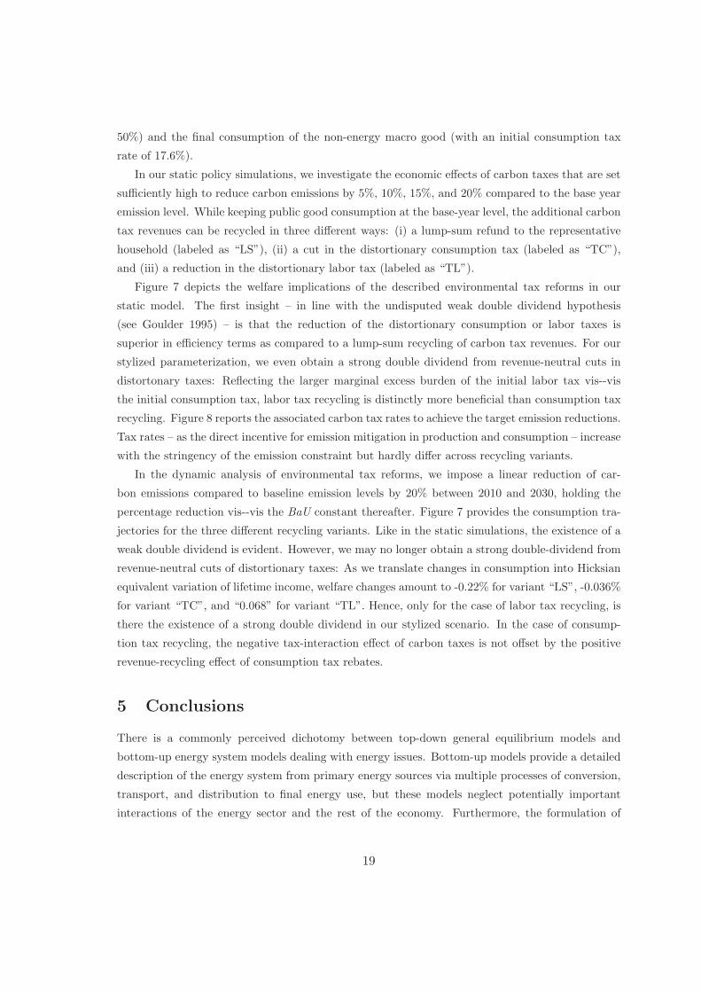
Figure 7 depicts the welfare implications of the described environmental tax reforms in our

static model. The first insight – in line with the undisputed weak double dividend hypothesis

(see Goulder 1995) – is that the reduction of the distortionary consumption or labor taxes is

superior in efficiency terms as compared to a lump-sum recycling of carbon tax revenues. For our

stylized parameterization, we even obtain a strong double dividend from revenue-neutral cuts in

distortonary taxes: Reflecting the larger marginal excess burden of the initial labor tax vis--vis

the initial consumption tax, labor tax recycling is distinctly more beneficial than consumption tax

recycling. Figure 8 reports the associated carbon tax rates to achieve the target emission reductions.

Tax rates – as the direct incentive for emission mitigation in production and consumption – increase

with the stringency of the emission constraint but hardly differ across recycling variants.

In the dynamic analysis of environmental tax reforms, we impose a linear reduction of car-

bon emissions compared to baseline emission levels by 20% between 2010 and 2030, holding the

percentage reduction vis--vis the BaU constant thereafter. Figure 7 provides the consumption tra-

jectories for the three different recycling variants. Like in the static simulations, the existence of a

weak double dividend is evident. However, we may no longer obtain a strong double-dividend from

revenue-neutral cuts of distortionary taxes: As we translate changes in consumption into Hicksian

equivalent variation of lifetime income, welfare changes amount to -0.22% for variant “LS”, -0.036%

for variant “TC”, and “0.068” for variant “TL”. Hence, only for the case of labor tax recycling, is

there the existence of a strong double dividend in our stylized scenario. In the case of consump-

tion tax recycling, the negative tax-interaction effect of carbon taxes is not offset by the positive

revenue-recycling effect of consumption tax rebates.

5 Conclusions

There is a commonly perceived dichotomy between top-down general equilibrium models and

bottom-up energy system models dealing with energy issues. Bottom-up models provide a detailed

description of the energy system from primary energy sources via multiple processes of conversion,

transport, and distribution to final energy use, but these models neglect potentially important

interactions of the energy sector and the rest of the economy. Furthermore, the formulation of

19

such models as mathematical programs restricts their direct applicability to integrable equilibrium

problems. Many interesting policy problems involving inefficiencies due to market distortions or

market failures can therefore not be handled – except by resorting to iterative optimization methods

(Rutherford (1999b)). Top-down general equilbrium models, on the other hand, are able to capture

market interactions and inefficiencies in a comprehensive manner but typically lack technological

details that might be relevant for the policy issue at hand.

In this paper, we have motivated the formulation of market equilibrium as a mixed complemen-

tarity problem to bridge the gap between bottom-up and top-down analysis. Through the explicit

representation of weak inequalities and complementarity between decision variables and equilib-

rium conditions, the complementarity approach allows an analyst to exploit the advantages of each

model type – technological details of bottom-up models and economic richness of top-down models

– in a single mathematical format.

Despite the coherence of the integrated complementarity approach, dimensionality may impose

limitations on its practical application. Bottom-up programming models of the energy system of-

ten involve a large number of bounds on decision variables. These bounds are treated implicitly

in mathematical programs but introduce unavoidable complexity in the integrated complementar-

ity formulation since they must be associated with explicit price variables in order to account for

income effects. Therefore, future research may be dedicated to decomposition approaches that per-

mit consistent combination of complex top-down models and large-scale bottom-up energy system

models for energy policy analysis.

20

References

Bahn, O., S. Kypreos, B. Bueler, and H. J. Luethi, “Modelling an international market of

CO2 emission permits,” International Journal of Global Energy Issues, 1999, 12, 283–291.

Bohringer, C., “The Synthesis of Bottom-Up and Top-Down in Energy Policy Modeling,” Energy

Economics, 1998, 20 (3), 233–248.

Bosetti, V., C. Carraro, M. Galeotti, E. Massetti, and M. Tavoni, “WITCH: A World

Induced Technical Change Hybrid Model,” Energy Journal – Special Issue, 2006, pp. 13–38.

Brooke, A., D. Kendrick, and A. Meeraus, GAMS: A Users Guide, GAMS Development

Corp., 1996.

Dimaranan, B. V. and R.A. Dougall, “Global trade, assistance, and production: The GTAP

6 Data Base,” Technical Report, Center for Global Trade Analysis, Purdue University 2006.

Dirkse, S. and M. Ferris, “The PATH Solver: A Non-monotone Stabilization Scheme for Mixed

Complementarity Problems,” Optimization Methods & Software, 1995, 5, 123–156.

Drouet, L., A. Haurie, M. Labriet, P. Thalmann, M. Vielle, and L. Viguier, “A Coupled

Bottom-up / Top-Down Model for GHG Abatement Scenarios in the Swiss Housing Sector,”

in R. Loulou, J. P. Waaub, and G. Zaccour, eds., Energy and Environment, Cambridge, 2005,

pp. 27–62.

European Commission (EC), Directive 2001/77/EC on the Promotion of Electricity produced

from Renewable Energy Sources (RES-E) in the internal electricity market 2001.

Goulder, L. H., “Environmental taxation and the double dividend: A readers guide,” Interna-

tional Tax and Public Finance, 1995, 2, 157–183.

Hofman, K. and D. Jorgenson, “Economic and technological models for evaluation of energy

policy,” The Bell Journal of Economics, 1976, pp. 444–446.

Hogan, W. W. and J. P. Weyant, “Combined Energy Models,” in J. R. Moroney, ed., Advances

in the Economics of Energy and Ressources, 1982, pp. 117–150.

Hourcade, J.-C., M. Jaccard, C. Bataille, and F. Gershi, “Hybrid Modeling: New Answers

to Old Challenges,” Energy Journal–Special Issue, 2006, pp. 1–12.

Hurwicz, L., “What is the Coase Theorem?,” Japan and the World Economy, 1999, 7, 49–75.

IEA, Nuclear Power in the OECD 2001. Available at:

http://www.iea.org/textbase/nppdf/free/2000/nuclear2001.pdf.

King, B., “What is a SAM?,” in “Social Accounting Matrices: A Basis for Planning,” Washington

D. C.: The World Bank, 1985.

Lau, M., A. Pahlke, and T. F. Rutherford, “Approximating Infinite-horizon Models in a

Complementarity Format: A Primer in Dynamic General Eqilibrium Analysis,” Journal of

Economic Dynamics and Control, 2002, 26, 577–609.

21

Manne, A. S., “ETA-MACRO: A Model of Energy Economy Interactions,” Technical Report,

Electric Power Research Institute, Palo Alto, California 1977.

Manne, A.S., R. Mendelsohn, and R.G. Richels, “MERGE: A Model for Evaluating Regional

and Global Effects of GHG Reduction Policies,” Energy Policy, 2006, 23, 17–34.

Mathiesen, L., “Computation of Economic Equilibrium by a Sequence of Linear Complementarity

Problems,” in A. Manne, ed., Economic Equilibrium - Model Formulation and Solution, Vol. 23

1985, pp. 144–162.

Messner, S. and L. Schrattenholzer, “MESSAGE-MACRO: Linking an Energy Supply Model

with a Macroeconomic Module and Solving Iteratively,” Energy – The International Journal,

2000, 25 (3), 267–282.

and M. Strubegger, “Ein Modellsystem zur Analyse der Wechselwirkungen zwischen En-

ergiesektor und Gesamtwirtschaft,” Offentlicher Sektor – Forschungsmemoranden, 1987, 13,

1–24.

OECD, Database on environmentally related taxes in OECD countries 2001. Available at:

http://www.oecd.org/env/policies/taxes/index.htm.

Pressman, I., “A Mathematical Formulation of the Peak-Load Problem,” The Bell Journal of

Economics and Management Science, 1970, 1, 304–326.

Russell, T., “Aggregation, Heterogeneity, and the Coase Invariance Theorem,” Japan and the

World Economy, 1999, 7, 105–111.

Rutherford, T. F., “Extensions of GAMS for Complementarity Problems Arising in Applied

Economics,” Journal of Economic Dynamics and Control, 1995, 19, 1299–1324.

, “Applied General Equilibrium Modelling with MPSGE as a GAMS Subsystem: An Overview

of the Modelling Framework and Syntax,” Computational Economics, 1999, 14, 1–46.

, “Sequential Joint Maximization,” in J.Weyant, ed., Energy and Environmental Policy Mod-

eling, Vol. 18, Kluwer, 1999, chapter 9.

Schafer, A. and H.D. Jacoby, “Experiments with a Hybrid CGE-Markal Model,” Energy Jour-

nal – Special Issue, 2006, pp. 171–178.

Schumacher, K. and R.D. Sands, “Where are the Industrial Technologies in Energy-Economy

Models? – An Innovative CGE Approach for Steel Production in Germany,” Discussion Paper

No. 605, DIW, Berlin 2006.

Takayma, T. and G. G. Judge, Spatial and Temporal Price and Allocation Models, Amsterdam:

North-Holland, 1971.

22

Table 1: Illustrative Base Year Equilibrium Data Set (bn. $)

Y COA GAS OIL ELE RA

Y 30864 -36 -71 -216 -267 -30274COA -12 105 -15 -78GAS -83 249 -33 -15 -47OIL -721 -2 1151 -61 -367ELE -746 -6 -4 -23 1126 -347Labor -17088 -20 -35 -141 -180 17464Capital -12214 -17 -99 -434 -454 13218Rent -26 -38 -289 353Key: ROI: rest of industry, COA: coal, GAS: gas

OIL: oil, ELE: electricity, RA: household

Table 2: Elasticities of Substitution in Production and Final Demand

Value-added composite versus other inputs in macro-good production σY = 0.5

Fossil fuels in macro-good production σE = 2

Resource versus other inputs in fossil fuel production σCoal = 0.5

σOil = 0.25

σGas = 0.25

Energy versus non-energy inputs in final consumption σC = 0.75

Electricity versus non-electric energy in final consumption σCELE = 0.3

Table 3: Endowments (in bn. at $ unit prices)

Time endowment Z = 30562

Capital endowment K = 13218

Resource endowments in fossil fuels RCoal = 26

ROil = 38

RGas = 289

23

Table 4: Cost Structure of Technologies Active in the Base Year

coal gas oil nuclear hydroELE 437 215 83 186 205Y -106 -38 -7 -55 -61COA -78GAS -86OIL -61Labor -72 -26 -4 -37 -41Capital -181 -65 -11 -94 -103

Table 5: Cost Structure of Technologies Inactive in the Base Year

wind biomass solarELE 1 1 1Y -0.1 -0.5 -0.1Capital -0.9 -0.5 -1.8Labor -0.1 -0.3 -0.1Wind -1Trees -1Sun -1

24

-0.035

-0.03

-0.025

-0.02

-0.015

-0.01

-0.005

0

0 25 50 75 100

Equ

ival

ent v

aria

tion

(%)

Nuclear capacity reduction (% vis- -vis BaU)

Fossil No fossil

Figure 1: Static Welfare Effects of Nuclear Phase-Out

25

0

0.05

0.1

0.15

0.2

0.25

0.3

0.35

0.4

0.45

0 25 50 75 100

Act

ivity

leve

l of

tech

nolo

gies

(no

rmal

ized

uni

ts)

Nuclear capacity reduction (% vis- -vis BaU)

coalgas

oilnuclear

hydrowind

Figure 2: Static Technology Shifts in Power Production for Nuclear Phase-Out

26

-1.4

-1.2

-1

-0.8

-0.6

-0.4

-0.2

0

0.2

2010 2020 2030 2040 2050 2060 2070 2080 2090 2100

Cha

nge

from

BaU

(%

)

Time

Consumption Investment Electricity

Figure 3: Dynamic Impacts of Nuclear Phase-Out (Variant: “No Fossil”)

27

-0.07

-0.06

-0.05

-0.04

-0.03

-0.02

-0.01

0

0.01

18 20 22 24 26 28

Equ

ival

ent v

aria

tion

(%)

Green quota in % of overall electricity supply

Long run Short run

Figure 4: Static Welfare Effects of Green Quotas

28

-5

0

5

10

15

20

25

30

35

18 20 22 24 26 28

Subs

idy

rate

(%

of

elec

tric

ity p

rice

)

Green quota in % of overall electricity supply

Long run Short run

Figure 5: Static Subsidy Rates of Green Quotas

29

-0.5

0

0.5

1

1.5

2

2.5

3

3.5

2010 2020 2030 2040 2050 2060 2070 2080 2090 2100

Cha

nge

from

BaU

(%

)

Time

Consumption Investment Electricity

Figure 6: Dynamic Impacts of Green Quotas

30

-0.2

-0.15

-0.1

-0.05

0

0.05

0.1

0.15

18 20 22 24 26

Equ

ival

ent v

aria

tion

(%)

Carbon emission reduction (in % vis- -vis base year)

LS TC TL

Figure 7: Static Welfare Effects of Environmental Tax Reforms

31

0

5

10

15

20

25

30

35

40

45

18 20 22 24 26

Car

bon

tax

in $

per

ton

of C

Carbon emission reduction (in % vis- -vis base year)

LS TC TL

Figure 8: Static Carbon Tax Rates of Environmental Tax Reforms

32

-2

-1.5

-1

-0.5

0

0.5

1

2010 2020 2030 2040 2050 2060 2070 2080 2090 2100

Cha

nge

from

BaU

(%

)

Time

LS TC TL

Figure 9: Dynamic Consumption Effects of Environmental Tax Reforms

33