arX

iv:m

ath/

0107

067v

1 [

mat

h.D

S] 1

0 Ju

l 200

1 Information, complexity and entropy:

a new approach to theory and

measurement methods

Vieri Benci, Claudio Bonanno, Stefano Galatolo,

Giulia Menconi, Federico Ponchio

Dedicated to Giovanni Prodi who tought us to appreciateScience and Culture in Mathematics

Contents

1 Introduction 2

1.1 Information, complexity and entropy . . . . . . . . . . . . . . 21.2 Dynamical systems and chaos . . . . . . . . . . . . . . . . . . 41.3 Analysis of experimental data . . . . . . . . . . . . . . . . . . 6

2 Information content and complexity 7

2.1 Information content of finite strings . . . . . . . . . . . . . . . 72.2 Infinite strings and complexity . . . . . . . . . . . . . . . . . . 9

3 Dynamical Systems 12

3.1 Information and the Kolmogorov-Sinai entropy . . . . . . . . . 123.2 Computable partitions . . . . . . . . . . . . . . . . . . . . . . 143.3 Computable complexity of an orbit . . . . . . . . . . . . . . . 17

4 Numerical Experiments 18

4.1 The Manneville map . . . . . . . . . . . . . . . . . . . . . . . 184.2 The logistic map . . . . . . . . . . . . . . . . . . . . . . . . . 20

5 DNA sequences 23

1

1 Introduction

In this paper, we present some results on information, complexity and entropyas defined below and we discuss their relations with the Kolmogorov-Sinaientropy which is the most important invariant of a dynamical system. Theseresults have the following features and motivations:

• we give a new computable definition of information and complexitywhich allows to give a computable characterization of the K-S entropy;

• these definitions make sense even for a single orbit and can be measuredby suitable data compression algorithms; hence they can be used insimulations and in the analysis of experimental data;

• the asymptotic behavior of these quantities allows to compute not onlythe Kolmogorov-Sinai entropy but also other quantities which give ameasure of the chaotic behavior of a dynamical system even in the caseof null entropy.

1.1 Information, complexity and entropy

Information, complexity and entropy are words which in the mathematicaland physical literature are used with different meanings and sometimes evenas synonyms (e.g. the Algorithmic Information Content of a string is calledKolmogorov complexity; the Shannon entropy sometimes is confused withShannon information etc.). For this reason, an intuitive definition of thesenotions as they will be used in this paper will be given soon. In our approachthe notion of information is the basic one. Given a finite string s (namely afinite sequence of symbols taken in a given alphabet), the intuitive meaningof quantity of information I(s) contained in s is the following one:

I(s) is the length of the smallest binary message from which you canreconstruct s.

In his pioneering work, Shannon defined the quantity of information asa statistical notion using the tools of probability theory. Thus in Shannonframework, the quantity of information which is contained in a string dependson its context. For example the string ′the′ contains a certain informationwhen it is considered as a string coming from the English language. The samestring ′the′ contains much more Shannon information when it is consideredas a string coming from the Italian language because it is much rarer in theItalian language. Roughly speaking, the Shannon information of a string isthe absolute value of the logarithm of its probability.

2

However there are measures of information which depend intrinsically onthe string and not on its probability within a given context. We will adopt thispoint of view. An example of these measures of information is the AlgorithmicInformation Content (AIC). In order to define it, it is necessary to define thepartial recursive functions. We limit ourselves to give an intuitive idea whichis very close to the formal definition, so we can consider a partial recursivefunction as a computer C which takes a program p (namely a binary string)as an input, performs some computations and gives a string s = C(p), writtenin the given alphabet, as an output. The AIC of a string s is defined as theshortest binary program p which gives s as its output, namely

IAIC(s) = min|p| : C(p) = s

where |p| is the length of the string p. From an heuristic point of view, theshortest program p which outputs the string s is a sort of optimal encodingof s. The information that is necessary to reconstruct the string is containedin the program.

Another measure of the information content of a finite string can also bedefined by a lossless data compression algorithm Z which satisfies suitableproperties which will be discussed in Section 2.1. We can define the infor-mation content of the string s as the length of the compressed string Z(s),namely

IZ (s) = |Z(s)| .

The advantage of using a Compression Algorithm lies in the fact that,in this way, the information content IZ (s) turns out to be a computablefunction. For this reason we will call it Computable Information Content(CIC).

If ω is an infinite string, in general, its information is infinite; however itis possible to define another notion: the complexity. The complexity K(ω)of an infinite string ω is the mean information I contained in a digit of ω,namely

K(ω) = lim supn→∞

I(ωn)

n(1)

where ωn is the string obtained taking the first n elements of ω. If we equipthe set of all infinite strings Ω with a probability measure µ, then the entropyhµ of (Ω, µ) can be defined as the expectation value of the complexity:

hµ =

∫

Ω

K(ω) dµ . (2)

3

If I (ω) = IAIC (ω) or I (ω) = IZ (ω) , under suitable assumptions on Zand µ, hµ turns out to be equal to the Shannon entropy. Notice that, inthis approach, the probabilistic aspect does not appear in the definition ofinformation or complexity, but only in the definition of entropy.

1.2 Dynamical systems and chaos

Chaos, unpredictability and instability of the behavior of dynamical systemsare strongly related to the notion of information. The Kolmogorov-Sinai en-tropy can be interpreted as an average measure of information that is neces-sary to describe a step of the evolution of a dynamical system. The traditionaldefinition of the Kolmogorov-Sinai entropy is given by the methods of prob-abilistic information theory. It is the translation of the Shannon entropy intothe world of dynamical systems.

We have seen that the information content of a string can be defined eitherwith probabilistic methods or using the AIC or the CIC. Similarly also theK-S entropy of a dynamical system can be defined in different ways. Theprobabilistic method is the usual one, the AIC method has been introducedby Brudno [9]; the CIC method has been introduced in [15] and [3]. So, inprinciple, it is possible to define the entropy of a single orbit of a dynamicalsystem (which we will call, as sometimes it has already been done in theliterature, complexity of the orbit). There are different ways to do this (see[9], [14], [17], [7] , [16]). In this paper, we will introduce a method which canbe implemented in numerical simulations. Now we will describe it briefly.

Using the usual procedure of symbolic dynamics, given a partition α ofthe phase space of the dynamical system (X, µ, T ), it is possible to associatea string Φα (x) to the orbit having x as initial condition. If α = (A1, . . . , Al),then Φα (x) = (s0, s1, . . . , sk, . . . ) if and only if

T kx ∈ Ask ∀ k .

If we perform an experiment, the orbit of a dynamical system can bedescribed only with a given degree of accuracy, described by the partition ofthe phase space X . A more accurate measurement device corresponds to afiner partition of X. The symbolic orbit Φα (x) is a mathematical idealizationof these measurements. We can define the complexity K(x, α) of the orbitwith initial condition x with respect to the partition α in the following way

K(x, α) = lim supn→∞

I(x, α, n)

n

where

I(x, α, n) := I(Φα (x)n); (3)

4

here Φα (x)n represents the first n digits of the string Φα (x) . Letting α to

vary among all the computable partitions (see Section 4.1), we set

K(x) = supαK(x, α) .

The numberK(x) can be considered as the average amount of informationnecessary to ”describe” the orbit in the unit time when you use a sufficientlyaccurate measurement device.

Notice that the complexity of each orbit K(x) is defined independently ofthe choice of an invariant measure. In the compact case, if µ is an invariantmeasure on X then

∫

XK(x) dµ equals the Kolmogorov-Sinai entropy. In

other words, in an ergodic dynamical system, for almost all points x ∈ X, andfor suitable choice of α, I(x, α, n) ∼ hµn. Notice that this result holds for alarge class of Information functions I as for example the AIC and the CIC.Thus we have obtained an alternative way to understand of the meaning ofthe K-S entropy.

The above construction makes sense also for a non stationary system.Its average over the space X is a generalization of the K-S entropy to thenon stationary case. Moreover, the asymptotic behavior of I(x, α, n) givesan invariant of the dynamics which is finer than the K-S entropy and isparticularly relevant when the K-S entropy is null.

It is well known that the Kolmogorov-Sinai entropy is related to theinstability of the orbits. The exact relations between the K-S entropy andthe instability of the system is given by the Ruelle-Pesin theorem ([24]). Wewill recall this theorem in the one-dimensional case. Suppose that the averagerate of separation of nearby starting orbits is exponential, namely

∆x(n) ≃ ∆x(0)2λn for n≪ ∞

where ∆x(n) denotes the distance of these two points. The number λ is calledLyapunov exponent; if λ > 0 the system is instable and λ can be considered ameasure of its instability (or sensibility with respect to the initial conditions).The Ruelle-Pesin theorem implies that, under some regularity assumptions,λ equals the K-S entropy.

There are chaotic dynamical systems whose entropy is null: usually theyare called weakly chaotic. Weakly chaotic dynamics arises in the study of selforganizing systems, anomalous diffusion, long range interactions and manyothers. In such dynamical systems the amount of information necessary todescribe n steps of an orbit is less than linear in n, thus the K-S entropy is notsensitive enough to distinguish the various kinds of weakly chaotic dynamics.Nevertheless, using the ideas we presented here, the relation between initial

5

data sensitivity and information content of the orbits can be generalized tothese cases.

To give an example of such a generalization, let us consider a dynamicalsystem ([0, 1], T ) where the transition map T is constructive1, and the func-tion I(x, α, n) is defined using the AIC in a slightly different way than inSection 3 (see [16]). If the speed of separation of nearby starting orbits goeslike ∆x(n) ≃ ∆x(0)f(x, n), then for almost all the points x ∈ [0, 1] we have

I(x, α, n) ∼ log(f(x, n)).

In particular, if we have power law sensitivity ( ∆x(n) ≃ ∆x(0)np), theinformation content of the orbit is I(x, α, n) ∼ p log(n). If we have a stretchedexponential sensitivity ( ∆x(n) ≃ ∆x(0)2λn

p

, p < 1) the information contentof the orbits will increase with the power law: I(x, α, n) ∼ np.

An example of stretched exponential is provided by the Manneville map(see Section 4.1). The Manneville map is a discrete time dynamical systemwhich was introduced by [22] as an extremely simplified model of intermittentturbulence in fluid dynamics. The Manneville map is defined on the unitinterval to itself by T (x) = x+xz (mod 1). When z > 2 the Manneville mapis weakly chaotic and non stationary. It can be proved [17], [7], [16] that foralmost each x (with respect to the Lebesgue measure)

IAIC(x, α, n) ∼ n1

z−1 . (4)

1.3 Analysis of experimental data

By the previous considerations, the analysis of I(x, α, n) gives useful infor-mation on the underlying dynamics. Since I(x, α, n) can be defined throughthe CIC, it turns out that it can be used to analyze experimental datausing a compression algorithm which satisfies the property required by thetheory and which is fast enough to analyze long strings of data. We haveimplemented a particular compression algorithm we called CASToRe: Com-pression Algorithm Sensitive To Regularity. CASToRe is a modification ofthe LZ78 algorithm. Its internal running and the heuristic motivations forsuch an algorithm are described in the Appendix (see also [3]). We have usedCASToRe on the Manneville map and we have checked that the experimentalresults agree with the theoretical one, namely with equation (4) (Section 4.1;see also [3]). Then we have used it to analyze the behavior of I(x, α, n) forthe logistic map at the chaos threshold (Section 4.2, see also [8]).

1a constructive map is a map that can be defined using a finite amount of information,see [16].

6

Finally, we have applied CASToRe and the CIC analysis to DNA se-quences (Section 5), following the ideas of [1], [2], [10] for what concerns thestudy of the randomness of symbolic strings produced by a biological source.The cited authors performed some classical statistical techniques, so we hopethat our approach will give rise both to new answers and new questions.

2 Information content and complexity

2.1 Information content of finite strings

We clarify the definition of Algorithmic Information Content that was out-lined in the Introduction. For a more precise exposition see for example [12]and [28].

In the following, we will consider a finite alphabet A, a = #(A) is thecardinality of A, and the set Σ (A) of finite strings from A, that is Σ (A) =⋃∞

n=1An ∪ ∅. Finally, let A = ΩA be the set of infinite strings ψ = (ωi)i∈

with ωi ∈ A for each i.

Let

C : Σ(0, 1) → Σ(A)

be a partial recursive function. The intuitive idea of partial recursive functionis given in the Introduction. For a formal definition we refer to any textbookof recursion theory.

The Algorithmic Information Content IAIC(s, C) of a string s relative toC is the length of the shortest string p such that C(p) = s. The string p canbe imagined as a program given to a computing machine and the value C(p)is the output of the computation. We require that our computing machineis universal. Roughly speaking, a computing machine is called universal ifit can simulate any other machine (again, for a precise definition see anybook of recursion). In particular if U and U ′ are universal then IAIC(s, U) ≤IAIC(s, U

′) + const, where the constant depends only on U and U ′. Thisimplies that, if U is universal, the complexity of s with respect to U dependsonly on s up to a fixed constant and then its asymptotic behavior does notdepend on the choice of U .

As we said in the introduction, the shortest program which gives a stringas its output is a sort of ideal encoding of the string. The information whichis necessary to reconstruct the string is contained in the program.

Unfortunately this coding procedure cannot be performed by any algo-rithm. This is a very deep statement and, in some sense, it is equivalent to

7

the Turing halting problem or to the Godel incompleteness theorem. Thenthe Algorithmic Information Content is not computable by any algorithm.

However, suppose we have some lossless (reversible) coding procedureZ : Σ(A) → Σ(0, 1) such that from the coded string we can reconstructthe original string (for example the data compression algorithms that are inany personal computer). Since the coded string contains all the informationthat is necessary to reconstruct the original string, we can consider the lengthof the coded string as an approximate measure of the quantity of informationthat is contained in the original string.

Of course not all the coding procedures are equivalent and give the sameperformances, so some care is necessary in the definition of information con-tent. For this reason we introduce the notion of optimality of an algorithm Z,defined by comparing its compression ratio with a statistical measure of in-formation: the empirical entropy. This quantity which is related to Shannonentropy is defined below.

Let s be a finite string of length n. We now define Hl(s), the lth empirical

entropy of s. We first introduce the empirical frequencies of a word in thestring s: let us consider w ∈ Al, a string from the alphabet A with lengthl; let s(m1,m2) ∈ Am2−m1 be the string containing the segment of s startingfrom the m1-th digit up to the m2-th digit; let

σ(s(i+1,i+l), w) =

1 if s(i+1,i+l) = w0 otherwise

( 0 ≤ i ≤ n− l).

The relative frequency of w (the number of occurrences of the word wdivided by the total number of l-digit sub words) in s is then

P (s, w) =1

n− l + 1

n−l∑

i=0

σ(s(i+1,i+l), w).

This can be interpreted as the “empirical” probability of w relative to thestring s. Then the l-empirical entropy is defined by

Hl(s) = −1

l

∑

w∈Al

P (s, w) logP (s, w).

The quantity lHl(s) is a statistical measure of the average informationcontent of the l−digit long substring of s.

The algorithm Z is coarsely optimal if its compression ratio |Z(s)|/|s|tends to be less than or equal to Hk(s) for each k.

8

Definition 1. A compression algorithm Z is coarsely optimal if ∀k there isfk, with fk(n) = o(n), such that ∀s it holds

|Z(s)| ≤ |s|Hk(s) + fk(|s|) .

Remark 2. The universal coding algorithms LZ77 and LZ78 [19],[20] satis-fies Definition 1. For the proof see [23].

However if the empirical entropy of the string is null (weak chaos) theabove definition is not satisfying (see [23]), so we need an algorithm havingthe same asymptotic behavior of the empirical entropy. In this way even inthe weakly chaotic case our algorithm will give a meaningful measure of theinformation.

Definition 3. A compression algorithm Z is optimal if there is a constantλ such that ∀k there is a gk with gk(t) = o(t) such that ∀s it holds

|Z(s)| ≤ λ|s|Hk(s) + gk(|Z(s)|).

Definition 4. The information content of s with respect to Z is defined asIZ(s) = |Z(s)|.

It is not trivial to construct an optimal algorithm. For instance the wellknown Lempel-Ziv compression algorithms are not optimal ([23]). Howeverthe set of optimal compression algorithms is not empty. In [6] we give anexample of optimal compression algorithm that is similar to the the Kol-mogorov frequency coding algorithm which is used also in [9]. This compres-sion algorithm is not of practical use because of its computational complexity.To our knowledge the problem of finding a fast optimal compression algo-rithm is still open.

2.2 Infinite strings and complexity

Now we show how the various definitions of information content of finitestrings can be applied to define a notion of orbit complexity for dynamicalsystems. This idea has already been exploited by Brudno ([9]). However ourconstruction to achieve this goal is different: we use Computable InformationContent instead of the Algorithmic Information Content (as it was done in[15]) and computable partitions instead of open covers.

This modifications with respect to the Brudno’s definition have the ad-vantage to give a quantity which is the limit of computable function andhence it can be used in numerical experiments.

9

The relations we can prove between these notions and the entropy willbe useful as a theoretical support for the interpretation of the experimentaland numerical results. As in Brudno’s approach, we will obtain that in theergodic case the orbit complexity has a.e. the same value as the entropy. Thereader will notice that the results which we will explain in this section aremeaningful in the positive entropy case. The null entropy cases are harder todeal with, and they present many aspects which are not yet well understood.There are some results based on the AIC [16], but there are not theoreticalresults based on the CIC which, in general, are mathematically more involved.On the other hand, our definitions based on CIC make sense and the relativequantities can be computed numerically; in section 4, we will present somefacts based on numerical experiments.

First, let us consider a symbolic dynamical system (a dynamical systemon a set of infinite strings). A symbolic dynamical system is given by (Ω, µ, σ),where Ω = AN, that is ω ∈ Ω implies that ω is an infinite sequence (ωi)i∈Nof symbols in A, σ is the shift map

σ((ωi)i∈N) = (ωi+1)i∈N

and µ is an invariant probability measure on Ω. A symbolic dynamical systemcan be also viewed as an information source. For the purposes of this paperthe two notions can be considered equivalent.

The complexity of an infinite string ω is the average (over all the stringω) of the quantity of information which is contained in a single digit of ω (cfr(1)). The quantity of information of a string can be defined in different ways;by Statistics (empirical entropy), by Computer Science (Algorithmic Infor-mation Content) or by compression algorithms. This will give three measuresof the complexity of infinite strings; each of them presents different kind ofadvantages depending on the problem to which it is applied.

Let ω be an infinite string in Ω. Let ωn = (ω1 . . . ωn) be the string con-taining the first n digits of ω.

Definition 5. If ω ∈ Ω then the algorithmic information complexity of ω isthe average information content per digit

KAIC(ω) =limsupn→∞

IAIC(ωn)

n.

If Z is a compression algorithm we also define the computable complexity ofω as the asymptotic compression ratio of Z

KZ(ω) =limsupn→∞

|Z(ωn)|

n.

10

We also define the quantity H(ω). If ω is an infinite string, H(ω) is a sortof Shannon entropy of the single string.

Definition 6. By the definition of empirical entropy we define:

Hl(ω) =limsupn→∞

Hl(ωn)

and

H(ω) =liml→∞

Hl(ω).

The existence of this limit is proved in [20].The following proposition is a direct consequence of ergodicity (for the

proof see again [20]).

Proposition 7. If (Ω, µ, σ) is ergodic H(ω) = hµ(σ) (where hµ is the Kol-mogorov-Sinai entropy) for µ-almost each ω.

Moreover from the definition of coarse optimality it directly follows that:

Remark 8. If Z is coarsely optimal then for each k

KZ(ω) ≤ Hk(ω) ,

so that

KZ(ω) ≤ H(ω) .

Remark 9. As it is intuitive, the compression ratio of Z cannot be less thanthe average information per digit of the algorithmic information (see [15]):

∀s KZ(s) ≥ KAIC(s) .

Then we have the following result.

Theorem 10. If (Ω, µ, T ) is a symbolic dynamical system and µ is ergodic,then for µ-almost each ω

KZ(ω) = H(ω) = KAIC(ω) = hµ(T ) .

Proof. 1) We have that KZ(ω) ≥ KAIC(ω) and then by the Brudno theo-rem ([9]) KZ(ω) ≥ hµ(T ) for µ-almost each ω.

2) On the other hand, KZ(ω) ≤ H(ω) and by Proposition 7 H(ω) = hµfor µ almost each ω ∈ Ω.

11

3 Dynamical Systems

3.1 Information and the Kolmogorov-Sinai entropy

Now we consider a dynamical system (X, µ, T ), where X is a compact metricspace, T is a continuous map T : X → X and µ is a Borel probabilitymeasure on X invariant for T . If α = A1, . . . , An is a measurable partitionof X (a partition of X where the sets are measurable) then we can associateto (X, µ, T ) a symbolic dynamical system (Ωα, µα, σ) ( called a symbolicmodel of (X, T )). The set Ωα is a subset of 1, . . . , nN (the space of infinitestrings made of symbols from the alphabet 1, . . . , n). To a point x ∈ X itis associated a string ω = (ωi)i∈N = Φα(x) defined as

Φα(x) = ω ⇐⇒ ∀j ∈, T j(x) ∈ Aωj

and Ωα = ∪x∈X

Φα(x). The measure µ on X induces a measure µα on the

associated symbolic dynamical system. The measure is first defined on thecylinders2

C(ω(k,n)) = ω ∈ Ωα : ωi = ωi for k ≤ i ≤ n− 1

by

µα(C(ω(k,n))) = µ(∩n−1

k T−i(Aωi))

and then extended by the classical Kolmogorov theorem to a measure µα onΩα.

Definition 11. We define the complexity of the orbit of a point x ∈ X, withrespect to the partition α, as

KAIC(x, α) = KAIC(ω),

KZ(x, α) = KZ(ω),

where ω = Φα(x).

Theorem 12. If Z is coarsely optimal, (X, µ, T ) is an ergodic dynamicalsystem and α is a measurable partition of X, then for µ-almost all x

KZ(x, α) = hµ(T, α)

where hµ(T, α) is the metric entropy of (X, µ, T ) with respect to the measur-able partition α.

2We recall that ω(k,n) = (ωi)k≤i≤n = (ωk, ωk+1, . . . , ωn).

12

Proof. To a dynamical system (X, µ, T ) and a measurable partition αit is associated a symbolic dynamical system (Ωα, µα, σ) as seen before. If(X, µ, T ) is ergodic then (Ωα, µα, σ) is ergodic and hµ(T |α) on X equalshµα

(σ) on Ωα (see e.g.[9]). Now by Theorem 10 for almost all points in Ωα

KZ(ω) = hµα(Ωα, σ). If we consider QΩα

:= ω ∈ Ωα : KZ(ω) = hµα(Ωα, σ)

and Q := Φ−1α (QΩα

) we have

∀x ∈ Q KZ(x, α) = KZ(Φα(x)) = hµα(σ) = hµ(T |α) .

According to the way in which the measure µα is constructed we have µ(Q) =µα(QΩα

) = 1.

Let βi be a family of measurable partitions such that limi→∞

diam(βi) = 0.

If we consider lim supi→∞

KZ(x, βi) we have the following

Lemma 13. If (X, µ, T ) is compact and ergodic, then for µ-almost all pointsx ∈ X, lim sup

i→∞

KZ(x, βi) = hµ(T ).

Proof. The points for which KZ(x, βi) 6= hµ(T |βi) are a set of null measurefor each i (Theorem 12). When excluding all these points, we exclude (for eachi) a zero-measure set. For all the other points we have KZ(x, βi) = hµ(T |βi)and then lim sup

i→∞

KZ(x, βi) =lim supi→∞

hµ(T, βi). Since the diameter of the

partitions βi tends to 0, we have that lim supi→∞

hµ(T, βi) = hµ(T ) (see e.g. [18]

page 170), and the statement is proved.

Remarks. Theorem 12 and the above lemma show that if a system has aninvariant measure, its entropy can be found by averaging the complexity ofits orbits over the invariant measure. Then, as we saw in the introduction,the entropy may be alternatively defined as the average orbit complexity.However if we fix a single point, its orbit complexity is not yet well definedbecause it depends on the choice of a partition. It is not possible to getrid of this dependence by taking the supremum over all partitions (as in theconstruction of Kolmogorov entropy), because this supremum goes to infinityfor each orbit that is not eventually periodic (see [4]).

This difficulty may be overcome in two ways:1) by considering open covers instead of partitions. This approach was

proposed by Brudno [9]. Since the sets in an open cover can have non emptyintersection, a step of the orbit of x can be contained at time in more thanone open set of the cover. This implies that an orbit may have an infinite

13

family of possible symbolic codings, among which we choose the “simplestone”;

2) by considering only a particular class of partitions (that are computablein some sense that will be clarified later) and define the orbit complexity ofa point as the supremum of the orbit complexity over that class.

Brudno’s open cover construction is not suitable for computational pur-poses because the choice of the simplest coding in a big family is not practi-cally feasible.

On the other hand, the computable partition approach is the mathemat-ical formalization of what we do in computer simulations. We consider adynamical system (X, T ) and we choose a partition β, which is always com-putable when it is explicitly given (the formal definition will be given in nextsection). We consider the symbolic orbit of a point x ∈ X with respect to β:it is a single string and we measure its information content by some suitableuniversal coding algorithm.

3.2 Computable partitions

In this section we will give a rigorous definition of computable partition.This notion is based on the idea of computable structure which relates theabstract notion of metric space with computer simulations. Before givingthe formal definitions, few words are necessary to describe the intuitive ideaabout it. Many models of the real words use the notion of real numbers ormore in general the notion of complete metric spaces. Even if you consider avery simple complete metric space, as, for example, the interval [0, 1] it con-tains a continuum of elements. This fact implies that most of these elements(numbers) cannot be described by any finite alphabet. Nevertheless, in gen-eral, the mathematics of complete metric spaces is simpler than the ”discretemathematics” in making models and the relative theorems. On the otherhand the discrete mathematics allows to make computer simulations. A firstconnection between the two worlds is given by the theory of approximation.But this connection becomes more delicate when we need to simulate moresophisticated objects of continuum mathematics. For example an open coveror a measurable partition of [0, 1] is very hard to be simulated by computer;nevertheless, these notions are crucial in the definition of many quantitiesas e. g. the K-S entropy of a dynamical system or the Brudno complexityof an orbit. For this reason, we have introduced the notion of ”computablestructure” which is a new way to relate the world of continuous models withthe world of computer simulations.

To simplify notations in the following, we will denote by Σ the set of finitebinary strings in a finite alphabet. Σ is the mathematical abstraction of the

14

world of the ”computer”, or more in general is the mathematical abstractionof the ”things” which can be expressed by any language. We suppose thatthe real objects which we want to talk about are modeled by the elements ofa metric space (X, d). We want to interpret the objects of Σ as points of X.Thus, the first definition we need is the following one:

Definition 14. An interpretation function on (X, d) is a function Ψ : Σ0 →X such that Ψ(Σ) is dense in X. (Σ0 ⊂ Σ is supposed to be a recursive set,namely a set for which there is an algorithm which ”decides” wether a givenelement belongs to set or not).

For example, if X = [0, 1] , a possible choice of Ψ is the following one: ifs = s1 . . . sn ∈ Σ = Σ0 = Σ(0, 1), then

Ψ(s) =

n∑

i=1

si2−i. (5)

A point x ∈ X is said to be ideal if it is the image of some stringx = Ψ(s), s ∈ Σ. Clearly almost every point is not ideal; however, it ispossible to perform computations on these points since they can be approx-imated with arbitrary precision by ideal points, provided that the interpre-tation is consistent with the distance d. This consideration leads us to thenotion of ”computable interpretation”: an interpretation is ”computable” ifthe distance between ideal points is computable with arbitrary precision. Theprecise definition is the following:

Definition 15. A computable interpretation function on (X, d) is a functionΨ : Σ0 → X such that Ψ(Σ0) is dense in X and there exists a total recursivefunction D : Σ0 × Σ0× → such that ∀s1, s2 ∈ Σ, n ∈ N

|d(Ψ(s1),Ψ(s2))−D(s1, s2, n)| ≤1

2n.

If we take again X = [0, 1], we may have a different interpretation con-sidering a string in Σ as an ASCII string. In this case Σ0 is the set of ASCIIstrings which denote a rational number in [0, 1] . In this way we obtain a differ-ent computable interpretation Ψ : Σ0 → X which describes the same metricspace. For most practical purposes, these two computable interpretations areessentially equivalent: they represent the same computable structure. A com-putable structure on a separable metric space (X, d) is a class of equivalentcomputable interpretations;.two interpretations are said to be equivalent ifthe distance of ideal points is computable up to arbitrary precision.

15

Definition 16. Let Ψ1 : Σ1 → X and Ψ2 : Σ2 → X be two computableinterpretations in (X, d); we say that Ψ1 and Ψ2 are equivalent if there existsa total recursive function D∗ : Σ1 × Σ2 ×N → R, such that ∀s1, s2 ∈ Σ1 ×Σ2, n∈N:

|d(Ψ1(s1),Ψ2(s2))−D∗(s1, s2, n)| ≤1

2n.

Proposition 17. The relation defined by definition 16 is an equivalence re-lation.

For the proof of this proposition see [14].

Definition 18. A computable structure J on X is an equivalence class ofcomputable interpretations in X.

Many concrete metric spaces used in analysis or in geometry have a natu-ral choice of a computable structure. The use of computable structures allowsto consider algorithms acting over metric spaces and to define constructivefunctions between metric spaces (see [14] or [16]).

For example if X = R we can consider the interpretation Ψ : Σ → R

defined in the following way: if s = s1 . . . sn ∈ Σ then

Ψ(s) =∑

1≤i≤n

si2[n/2]−i. (6)

This is an interpretation of a string as a binary expansion of a number.Ψ is a computable interpretation, the standard computable structure on R.

Definition 19. Let X be a space with a computable structure I and Ψ ∈ I.A partition β = Bi is said to be computable if there exists a recursiveZ : Σ → such that for each s, Z(s) = j ⇐⇒ Ψ(s) ∈ Bj .

For example let us consider the following partition βs0,n = Bns0, X−Bn

s0with

Bns0= Ψ(s), D(s0, s, n+ 2) ≤

1

2n − Ψ(s), D(s0, s, n+ 2) >

1

2n.

We remark that if n goes to infinity, the diameter of the set Bns0

goes to0. Moreover since X is compact, for each n there is a finite set of stringsSn = s0, . . . , sk such that X = ∪s∈Sn

Bns . Since the join of a finite fam-

ily of computable partitions is computable, there is a family of partitionsαn = ∨s∈Sn

βs,n such that αn is for each n a finite computable partition andlimn→∞diam(αn) = 0. This will be used in the proof of the next theorem.

16

3.3 Computable complexity of an orbit

Using the notion of computable partition, it is possible to define the com-plexity of a single orbit just using notion given by information theory. Sincewe have to different notions of complexity of a srting (namely KAIC(s) andKZ(s)), we get two different notions of complexity of an orbit:

Definition 20. If (X, T ) is a dynamical system over a metric space (X, d)with a computable structure we define the computable complexity of the orbitof x as:

KAIC(x) = supKAIC(x, β) | β computable partition

KZ(x) = supKZ(x, β) | β computable partition.

Theorem 21. If (X, µ, T ) is a dynamical system on a compact space and µis ergodic, then for µ-almost each x,

KZ(x) = KAIC(x) = hµ(T )

Proof. By what it is said above we remark that for each ǫ there is acomputable partition with diameter less than ǫ. Since computable partitionsare a countable set, by lemma 13 we prove the statement.

The above theorem states that KAIC(x) and KZ(x) are the right quantityto be considered; in fact in dynamical systems which are stationary andergodic they coincide with the K-S entropy for a.e. x. However the basicpoint is that KZ(x),in principle, can be computed by a machine with anarbitrary accuracy.

We call the function KZ(x) computable complexity of an orbit. For sta-tionary and ergodic dynamical systems, it is equivalent to the K-S entropy;nevertheless, it has a broader applicability and it presents the following fea-tures:

• it is the limit of computable functions and it can be measured in realexperiments;

• it is independent of the invariant measure;

• it makes sense even if the space X is not compact;

• it makes sense even if the dynamics is not stationary.

17

4 Numerical Experiments

Weakly chaotic dynamical systems give symbolic orbits with null entropy.For these systems the behavior of the quantity of information that is con-tained in n steps of the symbolic orbit is less than linear. However there isa big difference between a periodic dynamical system and a sporadic one(for example the Manneville map, Section 4.1). In fact, the latter can havepositive topological entropy and sensitive dependence on initial conditions.

Thus it is important to have a numerical way to detect weak chaos andto classify the various kind of chaotic behavior.

We have implemented a particular compression algorithm which we calledCASToRe (Compression Algorithm, Sensitive To Regularity). Here we presentsome experiments. First we used CASToRe in the study of the Mannevillemap. The information behavior of the Manneville map is known by the worksof [17], [16], (where the AIC has been used), [7] . We will see that our me-thods, implemented by a computer simulation, give results which coincidewith the the theoretical predictions of the mentioned papers. In the secondexample, CASToRe is used to have a measure of the kind of chaotic behaviorof the logistic map at the chaos threshold. Previous numerical works from thephysics literature proved that the logistic map has power law data sensitivi-ty to initial conditions, which implies logarithmic growth of the quantity ofinformation. Our numerical results surely suggest that in such a dynamicalsystem the behavior of the quantity of information is below any power law,confirming the previous results.

4.1 The Manneville map

The Manneville map was introduced by Manneville in [22] as an exampleof a discrete dissipative dynamical system with intermittency, an alternationbetween long regular phases, called laminar, and short irregular phases, calledturbulent. This behavior has been observed in fluid dynamics experiments andin chemical reactions. Manneville introduced his map, defined on the intervalI = [0, 1] by

f(x) = x+ xz(mod 1) z > 1, (7)

to have a simple model displaying this complicated behavior (see Figure 1).His work has attracted much attention, and the dynamics of the Mannevillemap has been found in many other systems. We can find applications of theManneville map in dynamical approaches to DNA sequences ([1],[2]) and ionchannels ([25]), and in non-extensive thermodynamic problems ([11]).

18

0

0.2

0.4

0.6

0.8

1

0 0.2 0.4 0.6 0.8 1

Figure 1: The Manneville map f for z = 2

Gaspard and Wang ([17]) described the behavior of the algorithmic com-plexity of the Manneville map, and called such a behavior sporadicity. Amathematical study of this kind of behavior has been done in a more generalcontest ([7]) and using different methods ([16]).

Let’s consider the following partition of the interval [0, 1]. Let x0 be suchthat f(x0) = 1 and x0 6= 1 (see Figure 1), then we call A0 = (x0, 1] andA1 = [0, x0]. We can now recursively define points xk such that f(xk) =xk−1 and xk < xk−1. Then we consider the partition α = (Ak) where Ak =(xk, xk−1), for k ∈. We denote by IAIC(x, α, n) the Algorithmic InformationContent of a n-long orbit of the Manneville map with initial condition x,using the partition α. We have that the mean value of IAIC(x, α, n), withrespect to the Lebesgue measure l, on the initial conditions of the orbit isEl[IAIC(x, α, n)] ∼ np, with p = 1

z−1for z ≥ 2, and El[IAIC(x, α, n)] ∼ n for

z < 2.Experiments which have been performed by using the compression al-

gorithm CASToRe ([3]) confirm the theoretical results and prove that themethod related to the computable complexity are experimantally reliable.We considered a set of one hundred initial points, generated 107-long orbits,and applied the algorithm to the associated symbolic strings s. If we consid-ered the compression algorithm Z =CASToRe, we have that IZ(s) is a goodapproximation of IAIC(x, α, n).

In Table 1 we show the results. The first column is the value of theparameter z. The last column gives the results of the theory for the exponentof the asymptotic behavior of IAIC(x, α, n). The second and third column

19

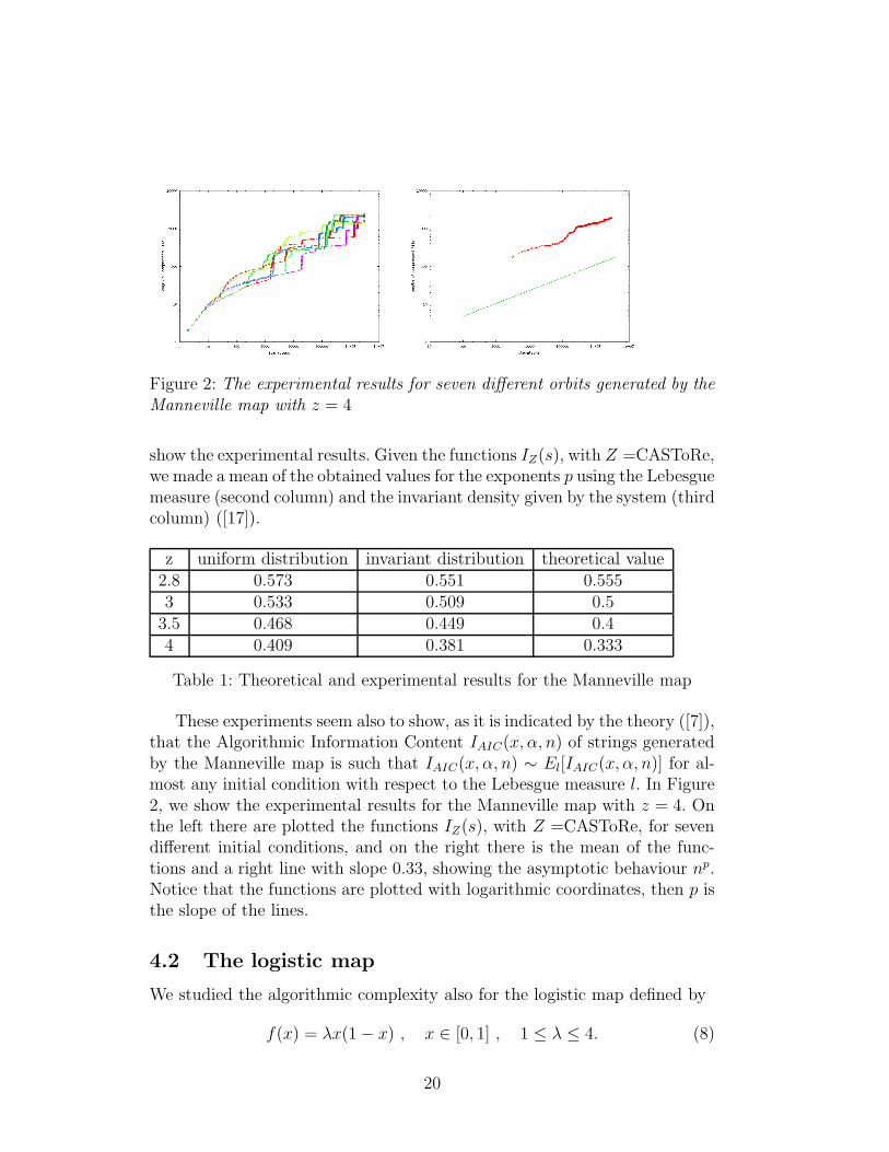
Figure 2: The experimental results for seven different orbits generated by theManneville map with z = 4

show the experimental results. Given the functions IZ(s), with Z =CASToRe,we made a mean of the obtained values for the exponents p using the Lebesguemeasure (second column) and the invariant density given by the system (thirdcolumn) ([17]).

z uniform distribution invariant distribution theoretical value2.8 0.573 0.551 0.5553 0.533 0.509 0.53.5 0.468 0.449 0.44 0.409 0.381 0.333

Table 1: Theoretical and experimental results for the Manneville map

These experiments seem also to show, as it is indicated by the theory ([7]),that the Algorithmic Information Content IAIC(x, α, n) of strings generatedby the Manneville map is such that IAIC(x, α, n) ∼ El[IAIC(x, α, n)] for al-most any initial condition with respect to the Lebesgue measure l. In Figure2, we show the experimental results for the Manneville map with z = 4. Onthe left there are plotted the functions IZ(s), with Z =CASToRe, for sevendifferent initial conditions, and on the right there is the mean of the func-tions and a right line with slope 0.33, showing the asymptotic behaviour np.Notice that the functions are plotted with logarithmic coordinates, then p isthe slope of the lines.

4.2 The logistic map

We studied the algorithmic complexity also for the logistic map defined by

f(x) = λx(1− x) , x ∈ [0, 1] , 1 ≤ λ ≤ 4. (8)

20

The logistic map has been used to simulate the behavior of biologicalspecies not in competition with other species. Later the logistic map hasalso been presented as the first example of a relatively simple map with anextremely rich dynamics. If we let the parameter λ vary from 1 to 4, wefind a sequence of bifurcations of different kinds. For values of λ < λ∞ =3.56994567187 . . . , the dynamics is periodic and there is a sequence of perioddoubling bifurcations which leads to the chaos threshold for λ = λ∞. Thedynamics of the logistic map at the chaos threshold has attracted muchattention and many are the applications of theories to the logistic map atthis particular value of the parameter λ. In particular, numerical experimentssuggested that at the chaos threshold the logistic map has null K-S entropy,implying that the sensitivity on initial conditions is less than exponential, andthere is a power-law sensitivity to initial conditions. These facts have justifiedthe application of generalized entropies to the map ([26],[27]). Moreover, fromthe relations between initial conditions sensitivity and information content([16]), we expect to find that the Algorithmic Information Content of thelogistic map at the chaos threshold is such that IAIC(s) ∼ log(n) for a n-digit long symbolic string s generated by one orbit of the map. We next showhow we have experimentally found this result.

From now on Z indicates the compression algorithm CASToRe. It isknown that for periodic maps the behavior of the Algorithmic InformationContent should be of order O(logn) for a n-long string, and it has beenproved that the compression algorithm CASToRe gives for periodic stringsIZ(s) ∼ Π(n) = log n log(logn), where we recall that IZ(s) is the binarylength of the compressed string ([8]). In Figure 3, we show the approxima-tion of IZ(s) with Π(n) for a 105-long periodic string of period 100.

We have thus used the sequence λn of parameters values where the pe-riod doubling bifurcations occur and used a “continuity” argument to obtainthe behavior of the information function at the chaos threshold. Another se-quence of parameters values µk approximating the critic value λ∞ from abovehas been used to confirm the results.

In Figure 4, we plotted the functions S(n) = IZ(s)Π(n)

for some values of thetwo sequences. The starred functions refer to the sequence µk and the othersto the sequence λn. The solid line show the limit function S∞(n). If we nowconsider the limit for n → +∞, we conjecture that S∞(n) converges to aconstant S∞, whose value is more or less 3.5. Then we can conclude that,at the chaos threshold, the Algorithmic Information Content of the logisticmap is IAIC(s) ≤ IZ(s) ∼ S∞Π(n). In particular we notice that we obtainedan Algorithmic Information Content whose order is smaller than any powerlaw, and we called this behavior mild chaos ([8]).

21

0

50

100

150

200

250

300

350

400

450

500

0 10000 20000 30000 40000 50000 60000 70000 80000 90000 100000

Figure 3: The solid line is the information function for a string σ of period100 compared with Π(N) plus a constant term

1

1.5

2

2.5

3

3.5

4

4.5

5

0 1e+06 2e+06 3e+06 4e+06 5e+06 6e+06 7e+06 8e+06 9e+06 1e+07

’S_23’’S_12’’S_14’’S_15’

’*S_17’’*S_19’’*S_20’

Figure 4: The solid line is the limit function S∞(n) and dashed lines are someapproximating functions from above (with a star) and below.

22

5 DNA sequences

We look at genomes as to finite symbolic sequences where the alphabet isthe one of nucleotides A, C, G, T and compute the complexity KZ (whereZ is the algorithm CASToRe) of some sequences or part of them.

DNA sequences, in fact, can be roughly divided in different functionalregions. First, let us analyze the structure of a Prokaryotic genome: a geneis not directly translated into protein, but is expressed via the productionof a messenger RNA. It includes a sequence of nucleotides that correspondsexactly with the sequence of amino acids in the protein (this is the so calledcolinearity of prokaryotic genes). These parts of the genome are the coding

regions. The regions of prokaryotic genome that are not coding are the noncoding regions: upstream and downstream regions, if they are proceedingor following the gene.

On the other hand, Eukaryotic DNA sequences have several non codingregions: a gene includes additional sequences that lie within the coding region,interrupting the sequence that represent the protein (this is why these areinterrupted genes). The sequences of DNA comprising an interrupted geneare divided into two categories:

• the exons are the sequences represented in the mature RNA and theyare the real coding region of the gene, that starts and ends with exons;

• the introns are the intervening sequences which are removed when thefirst transcription occurs.

So, the non coding regions in Eukaryotic genomes are intron sequencesand up/downstream sequences. The last two regions are usually called inter-

genic regions. In Bacteria and Viruses genomes, coding regions have moreextent than in Eukaryotic genomes, where non coding regions prevail.

There is a long-standing interest in understanding the correlation struc-ture between bases in DNA sequences. Statistical heterogeneity has beeninvestigated separately in coding and non coding regions: long-range correla-tions were proved to exist in intron and even more in intergenic regions, whileexons were almost indistinguishable from random sequences ([21],[10]). Ourapproach can be applied to look for the non-extensivity of the Informa-

tion content corresponding to the different regions of the sequences.We have used a modified version of the algorithm CASToRe, that exploits

a window segmentation (see Appendix); let L be the length of a window. Wemeasure the mean complexity of substrings with length L belonging to thesequence that is under analysis. Then, we obtain the Information and thecomplexity of the sequence as functions of the length L of the windows.

23

1.7

1.75

1.8

1.85

1.9

1.95

2

0 500000 1e+06 1.5e+06 2e+06

Com

plex

ity

Length of window

’H_coliCOD’’Hrand_coliCOD’

1.7

1.75

1.8

1.85

1.9

1.95

2

0 50000 100000 150000 200000 250000 300000 350000 400000 450000

Com

plex

ity

Length of window

’H_coliUP’’Hrand_coliUP’

Figure 5: On the left, the complexity of coding sequences of Bacterium Es-cherichia Coli as a function of the length L of the windows are compared to astatistically equivalent random sequence. On the right, the same comparisonwith respect to the intergenic (non coding) sequence of the same genome.

1.7

1.75

1.8

1.85

1.9

1.95

2

0 50000 100000 150000 200000

Com

plex

ity

Length of window

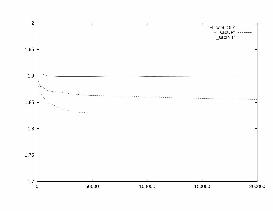
’H_sacCOD’’H_sacUP’’H_sacINT’

Figure 6: The analysis of the three functional regions of the genome of Eu-karyote Saccharomyces Cerevisiae: the solid line is relative to the coding re-gions, the dashed line to the intergenic regions, the dotted line to the intronregion. The complexities, as functions of length L of the windows, are clearlydifferent from each other. The regions have not similar length so the picturehas been drawn according to the shortest region.

24

In analogy with physical language, we call a function f extensive if thesum of the evaluations of f on each part of a partition of the domain equalsthe evaluation of f on the whole domain:

∑

i∈I

f(Ai) = f

(

⋃

i∈I

Ai

)

.

In case of a non-extensive function f , we have that the average on thedifferent parts underestimates the evaluation on the whole domain:

∑

i∈I

f(Ai) ≤ f

(

⋃

i∈I

Ai

)

.

Now let us consider the Information Content: each set Ai is a window offixed length L in the genome, so it can be considered as Ai(L). Then the

related complexity is IZ(Ai(L))L

.If a sequence is chaotic or random, then its Information content is exten-

sive, because it has no memory (neither short-range or long range correla-tions). But if a sequence shows correlations, then the more long-ranged thecorrelations are the more non-extensive is the related Information content.We have that:

• if the Information content is extensive, the complexity is constant as alinear function of the length L;

• if the Information content is non-extensive, the complexity is a decreas-ing, less than linear function of the length L.

From the experimental point of view, we expect our results to show thatin coding regions the Information content is extensive, while in non codingregions the extensivity is lost within a certain range [0, L∗] of window length(the number L∗ depends on the genome). This is also supported by thestatistical results exposed above.

In coding sequences, we found that the complexity is almost constant:the compression ratio does not change sensitively with L. In non codingsequences, the complexity decreases until some appropriate L∗ is reachedand later the compression ratio is almost constant.

This is an information-theoretical proof (alternative to the statistical tech-nique) that coding sequences are more chaotic than non coding ones. Figure5 shows the complexity of coding (on the left) and non coding (on the right)regions of the genome of Bacterium Escherichia Coli as a function of the

25

length L of the windows and compared with statistically equivalent randomsequences. Clearly the compression ratio decreases more in the non codingregions than in the coding ones, where the random sequences show almostconstant complexity.

Figure 6 shows the analysis of the three functional regions of the genomeof Saccharomyces Cerevisiae which is an eukaryote: the complexities, as func-tions of length L of the windows, are clearly different from each other. Weremark that the lower is the compression ratio, the higher is the aggregationof the words in the genome. This is due to the fact that the algorithm CAS-ToRe recognizes patterns already read, so it is not necessary to introduce newwords, but coupling old words to give rise to a new longer one is sufficient toencode the string.

Appendix: CASToRe

The Lempel-Ziv LZ78 coding scheme is traditionally used to codify a stringaccording to a so called incremental parsing procedure [20]. The algorithmdivides the sequence in words that are all different from each other and whoseunion is the dictionary. A new word is the longest word in the charstreamthat is representable as a word already belonging to the dictionary togetherwith one symbol (that is the ending suffix).

We remark that the algorithm LZ78 encodes a constant n digits longsequence ′111 . . .′ to a string with length about const + n

1

2 bits, while thetheoretical Information IAIC is about const + log n. So, we can not expectthat LZ78 is able to distinguish a sequence whose Information grows like nα

(α < 12) from a constant or periodic one.

This is the main motivation which lead us to create the new algorithmCASToRe. It has been proved in [8] that the Information of a constant se-quence, originally with length n, is 4 + 2 log(n + 1)[log(log(n + 1)) − 1], ifCASToRe is used. As it has been showed in section 4.1, the new algorithmis also a sensitive device to weak dynamics.

CASToRe is an encoding algorithm based on an adaptive dictionary.Roughly speaking, this means that it translates an input stream of sym-bols (the file we want to compress) into an output stream of numbers, andthat it is possible to reconstruct the input stream knowing the corrispondencebetween output and input symbols. This unique corrispondence between se-quences of symbols (words) and numbers is called the dictionary.

“Adaptive” means that the dictionary depends on the file under compres-sion, in this case the dictionary is created while the symbols are translated.

At the beginning of encoding procedure, the dictionary is empty. In order

26

to explain the principle of encoding, let’s consider a point within the encodingprocess, when the dictionary already contains some words.

We start analyzing the stream, looking for the longest word W in thedictionary matching the stream. Then we look for the longest word Y inthe dictionary where W + Y matches the stream. Suppose that we are com-pressing an english text, and the stream contains “basketball ...”, we mayhave the words “basket” (number 119) and “ball” (number 12) already inthe dictionary, and they would of course match the stream.

The output from this algorithm is a sequence of word-word pairs (W, Y),or better their numbers in the dictionary, in our case (119, 12). The resultingword “basketball” is then added to the dictionary, so each time a pair isoutput to the codestream, the string from the dictionary corresponding toW is extended with the word Y and the resulting string is added to thedictionary.

A special case occurs if the dictionary doesn’t contain even the startingone-character string (for example, this always happens in the first encodingstep). In this case we output a special code word which represents the nullsymbol, followed by this character and add this character to the dictionary.

Below there is an example of encoding, where the pair (4, 3), is composedfrom the fourth word ′AC′ and the third word ′G′.

ACGACACGGAC

word 1: (0, A) –> Aword 2: (0, C) –> Cword 3: (0, G) –> Gword 4: (1, 2) –> ACword 5: (4, 3) –> ACGword 6: (3, 4) –> GACThis algorithm can be used in the study of correlations.A modified version of the program can be used for study of correlations

in the stream: it partition the stream into fixed size segments and proceed toencode them separately. The algorithm takes advantage of replicated parts inthe stream. Limiting the encoding to each window separately, could resultsin longer total encoding. The difference between the length of the wholestream encoded and the sum of the encoding of each window depends onnumber of correlation between symbols at distance greater than the sizeof the window. Using different window sizes it is possible to construct a”spectrum” of correlation.

This has been applied for example on DNA sequences for the study ofmid and long-term correlations (see section 5).

27

Implementation:

The main problem implementing this algorithm is building a structurewhich allows to efficently search words in the dictionary. To this purpose, thedictionary is stored in a treelike structure where each node is a word X = (W,Y), its parent node being W, and storing a link to the string representingY. Using this method, in order to find the longest word in the dictionarymaching exactly a string, you need only to follow a branching path from theroot of the dictionary tree.

References

[1] Allegrini P., Barbi M., Grigolini P., West B.J., “Dynamical model forDNA sequences”, Phys. Rev. E, 52, 5281-5297 (1995).

[2] Allegrini P., Grigolini P., West B.J., “A dynamical approach to DNAsequences”, Phys. Lett. A, 211, 217-222 (1996).

[3] Argenti F., Benci V., Cerrai P., Cordelli A., Galatolo S., Menconi G.,“Information and dynamical systems: a concrete measurement on spo-radic dynamics”, to appear in Chaos, Solitons and Fractals (2001).

[4] Batterman R., White H., “Chaos and algorithmic complexity”, Found.Phys. 26, 307-336 (1996).

[5] Benci V., “Alcune riflessioni su informazione, entropia e complessita”,Modelli matematici nelle scienze biologiche, P.Freguglia ed., Quattro-Venti, Urbino (1998).

[6] Benci V., Bonanno C., Galatolo S., Menconi G., Ponchio F., Work inpreparation (2001).

[7] Bonanno C., “The Manneville map: topological, metric and algorithmicentropy”, work in preparation (2001).

[8] Bonanno C., Menconi G., “Computational information for the logisticmap at the chaos threshold”, arXiv E-print no. nlin.CD/0102034 (2001).

[9] Brudno A.A., “Entropy and the complexity of the trajectories of a dy-namical system”, Trans. Moscow Math. Soc. 2, 127-151 (1983).

[10] Buiatti M., Acquisti C., Mersi G., Bogani P., Buiatti M., “The bio-logical meaning of DNA correlations”, Mathematics and Biosciences ininteraction, Birkhauser ed., in press (2000).

28

[11] Buiatti M., Grigolini P., Palatella L., “Nonextensive approach to theentropy of symbolic sequences”, Physica A 268, 214 (1999).

[12] Chaitin G.J., Information, randomness and incompleteness. Papers onalgorithmic information theory., World Scientific, Singapore (1987).

[13] Galatolo S., “Pointwise information entropy for metric spaces”, Nonlin-earity 12, 1289-1298 (1999).

[14] Galatolo S., “Orbit complexity by computable structures”, Nonlinearity13, 1531-1546 (2000).

[15] Galatolo S., “Orbit complexity and data compression”, Discrete and Con-tinuous Dynamical Systems 7, 477-486 (2001).

[16] Galatolo S., “Orbit complexity, initial data sensitivity and weakly chaoticdynamical systems”, arXiv E-print no. math.DS/0102187 (2001).

[17] Gaspard P., Wang X.J., “Sporadicity: between periodic and chaotic dy-namical behavior”, Proc. Natl. Acad. Sci. USA 85, 4591-4595 (1988).

[18] Katok A., Hasselblatt B., Introduction to the Modern Theory of Dynam-ical Systems, Cambridge University Press (1995).

[19] Lempel A., Ziv A., “A universal algorithm for sequential data compres-sion” IEEE Trans. Information Theory IT 23, 337-343 (1977).

[20] Lempel A., Ziv J., “Compression of individual sequences via variable-rate coding”, IEEE Transactions on Information Theory IT 24, 530-536(1978).

[21] Li W., “The study of DNA correlation structures of DNA sequences: acritical review”, Computers chem. 21, 257-271 (1997).

[22] Manneville P., “Intermittency, self-similarity and 1/f spectrum in dissi-pative dynamical systems”, J. Physique 41, 1235-1243 (1980).

[23] Kosaraju S. Rao, Manzini G., “Compression of low entropy strings withLempel-Ziv algorithms”, SIAM J. Comput. 29, 893-911 (2000).

[24] Pesin Y.B., “Characteristic Lyapunov exponents and smooth ergodic the-ory”, Russ. Math. Surv. 32, PAGINE (1977).

[25] Toth T.I., Liebovitch L.S., “Models of ion channel kinetics with chaoticsubthreshold behaviour” Z. Angew. Math. Mech. 76, Suppl. 5, 523-524(1996).

29

[26] Tsallis C., “Possible generalization of Boltzmann-Gibbs statistics”, J.Stat. Phys. 52, 479 (1988).

[27] Tsallis C., Plastino A. R., Zheng W.M., “Power-law sensitivity to initialconditions - new entropic representation”, Chaos Solitons Fractals 8,885-891 (1997).

[28] Zvorkin A.K., Levin L.A., “The complexity of finite objects and thealgorithmic-theoretic foundations of the notion of information and ran-domness”, Russ. Math. Surv. 25, PAGINE (1970).

30

1.7

1.75

1.8

1.85

1.9

1.95

2

0 500000 1e+06 1.5e+06 2e+06 2.5e+06 3e+06

Com

plex

ity

Length of window

’H_coliCOD’’H_sacCOD’’H_c.elCOD’

1.7

1.75

1.8

1.85

1.9

1.95

2

0 50000 100000 150000 200000 250000 300000 350000 400000 450000

Com

plex

ity

Length of window

’H_coliUP’’H_sacUP’’H_c.elUP’

1.7

1.75

1.8

1.85

1.9

1.95

2

0 500000 1e+06 1.5e+06 2e+06

’H_coliCOD’’Hrand_coliCOD’

1.7

1.75

1.8

1.85

1.9

1.95

2

0 50000 100000 150000 200000 250000 300000 350000 400000 450000 500000

’H_coliUP’’Hrand_coliUP’

1.7

1.75

1.8

1.85

1.9

1.95

2

0 1e+06 2e+06 3e+06 4e+06 5e+06 6e+06 7e+06

’H_sacCOD’’Hrand_sacCOD’

1.7

1.75

1.8

1.85

1.9

1.95

2

0 10000 20000 30000 40000 50000

’H_sacINT’’Hrand_sacINT’

1.7

1.75

1.8

1.85

1.9

1.95

2

0 500000 1e+06 1.5e+06 2e+06 2.5e+06 3e+06

’H_sacUP’’Hrand_sacUP’

1.7

1.75

1.8

1.85

1.9

1.95

2

0 50000 100000 150000 200000 250000 300000 350000 400000 450000 500000

’H_coliUP’’H_sacUP’’H_c.elUP’

1.7

1.75

1.8

1.85

1.9

1.95

2

0 50000 100000 150000 200000

’H_sacCOD’’H_sacUP’’H_sacINT’