Improved Two-Sample Comparisons for Bounded Data

Jianning Kong

Shandong University

Jason Parker

Michigan State University

Donggyu Sul

University of Texas at Dallas

Abstract

The goal of this paper is to establish new testing procedures for comparing two

independent and bounded samples. The paper begins with a brief literature review

of the best traditional tests available. These tests are then applied to two canonical

examples of bounded data in public good games, revealing the problems of these tra-

ditional methods. Next, a new test for equal distributions is constructed using the

sample moments, since the moments determine a bounded distribution up to unique-

ness. When the underlying distributions of the two samples are beta, testing for equal

�rst and second moments becomes equivalent to testing for equal distributions. This

paper shows that the bootstrapped one-sample Kolmogorov-Smirnov test can be used

for testing the null that the sample is drawn from the beta distribution. Next, a new

central tendency test is developed using skewness. These newly-developed methods

are found to perform well in the �nite sample through Monte Carlo simulation and

through application to the canonical examples.

Key Words: Distributional Comparisons, Beta Distribution, Bounded Data, Skewness,

Rank Sum Test.

JEL Classi�cation Numbers: C12, C16, C23

1

1 Introduction

This paper addresses the comparison of two independent and bounded samples. The latter

restriction is a new addition to this literature that sharpens the statistical comparison,

allowing researchers to test more accurately. In many situations, the data can be normalized

to be bounded between zero and one. For example, in public good games and ultimatum

games, the experimental data are all bounded on the unit interval. Auction data are also

usually bounded in this way.

When data are bounded between zero and one, we will demonstrate that skewness can

be another measure of central tendency since the skewness combines information from the

mean and median. It is easy to show that the mean and median must be equal to 0.5 when

bounded samples are symmetric. Otherwise, the distribution becomes asymmetric, and the

mean may not be a good measure for central tendency. Meanwhile, the median may be

a better measure for central tendency with an extremely asymmetrically distributed and

unbounded sample, but with a bounded sample, the skewness can be an alternative measure

for central tendency since by de�nition, skewness measures where the mass of a distribution

is located.

Another interesting question is whether or not the underlying distribution of a bounded

sample is a beta distribution. This question is interesting for two reasons. First, theoretical

economists can use this information when they analyze the behavior of the subjects in

experimental games. Many empirical and theoretical papers have used the beta distribution

for their analyses (e.g., Bajari and Horta�csu, 2005; McKelvey and Palfrey, 1992). Second,

two-sample comparisons are much more straightforward when the two samples are drawn

from beta distributions. By estimating the two underlying parameters, � and �; various

test statistics can be constructed and their tests performed. Since additional information

about the distribution is used, these newly-designed methods have better power in the �nite

sample.

There are several goodness-of-�t tests available for testing whether or not a random vari-

able is generated from a reference distribution. Among them, the Kolmogorov-Smirnov (KS

hereafter) nonparametric test has been commonly used. When the underlying parameters

are estimated, the critical value for the KS test is generally unknown and requires a bootstrap

procedure. (See Babu and Rao, 2004; Meintanis and Swanepoel, 2007). We will show that

2

many laboratory experimental data sets are well characterized by a simple beta distribution.

Under the assumption that the underlying distributions of the two samples are beta, the

null hypothesis of equal distributions can be re-fomulated by using the two beta parameters, �

and �. Once these two parameters are estimated, each of the moments can also be estimated

since all of the moments are functions of � and �. The equality of means, medians, and

skewness tests are developed based on the estimates of these � and �; and their �nite sample

performance is examined. For the case when the two samples are not beta distributed, we also

derive the limiting distributions of the proposed tests for equal distributions and skewness.

The rest of the paper consists of four sections. The next section provides a short literature

review of the two-sample comparison literature, particularly focusing on the Wilcoxon-Mann-

Whitney (1945,1947, WMW hereafter) rank sum test, which has been used to test for equal

distributions. Section 3 provides new test statistics and testing procedures for the comparison

of two samples under the boundedness condition; it also introduces the beta distribution.

In Section 4, the new tests are extended parametrically via the beta distribution to further

increase the power of the tests. Section 5 examines the �nite sample properties of the new

tests by means of Monte Carlo simulation and provides an empirical demonstration. Section

6 concludes. Technical derivations and proofs are provided in appendices.

2 Preliminary and Canonical Empirical Examples

Here, we brie y discuss the statistical properties of the tests which are most popularly used in

practice. Then we demonstrate the problems of these tests by using real empirical examples.

2.1 Preliminary

We consider two continuous independent samples X = fx1; :::; xmg and Y = fy1; :::; yngwhere X � i:i:d: QX and Y � i:i:d: QY . Denote N = m+ n: The most popularly used tests

are the standard z-score, the WMW, and the KS tests. Here, we brie y review the latter

two tests.

The one-sample KS test is designed for detecting whether or not the sample of interest is

generated from a particular distribution. Let the empirical cumulative distribution function

be Fn and its true cumulative distribution function (CDF) be F: Then, the one-sample KS

3

statistic, dn; is de�ned as

dn = supx

���Fn (x)� F (x)��� :Under the null hypothesis, the KS statistic, d; converges to zero in probability as n ! 1,andpnd converges to the Kolmogorov distribution which does not depend on the function

F: However, in practice, the CDF of F (x) is usually evaluated with the estimated parame-

ters. For example, in the case of the normal distribution, the mean and variance should be

estimated from the sample. In this case, the critical value of dn must be obtained either by

a numerical approximation or by bootstrap. We will use this one-sample KS test to detect

whether or not the random samples are each generated from a beta distribution later. The

power of the one-sample KS test is much better than that of the two-sample KS test, which

we consider below.

The two-sample KS test is designed for testing whether or not the two samples are

generated from the same probability density function. The two-sample KS statistic, dn;m; is

de�ned as

dn;m = supx

���Fn (x)� Fm (x)��� :The asymptotic critical value can be obtained by approximation to the beta distribution.

See Zhang and Wu (2002) for a more detailed discussion. In practice, the two-sample KS

test has not been used popularly due to its lack of power. See Marsh (2010) for a �nite

sample comparison of various tests.

In practice, empirical researchers have used the WMW's rank sum test for testing the

equality of two distributions. In fact, Mann and Whitney (1947) clearly states that the null

hypothesis of the Wilcoxon (1945) test is the equality of two distributions. However, Chung

and Romano (2013) recently showed that the null hypothesis of the WMW test is not equal

distributions; instead the null should be written as

Hw0 : Pr (X � Y ) = 1=2: (1)

Note that Hw0 can be interpreted as the median of the di�erence of the two samples is zero.Meanwhile, the null hypothesis of equal distributions is given by

HQ0 : QX = QY : (2)

Obviously, if HQ0 is true, then Hw0 is true. However, the opposite is not true. Chung and

4

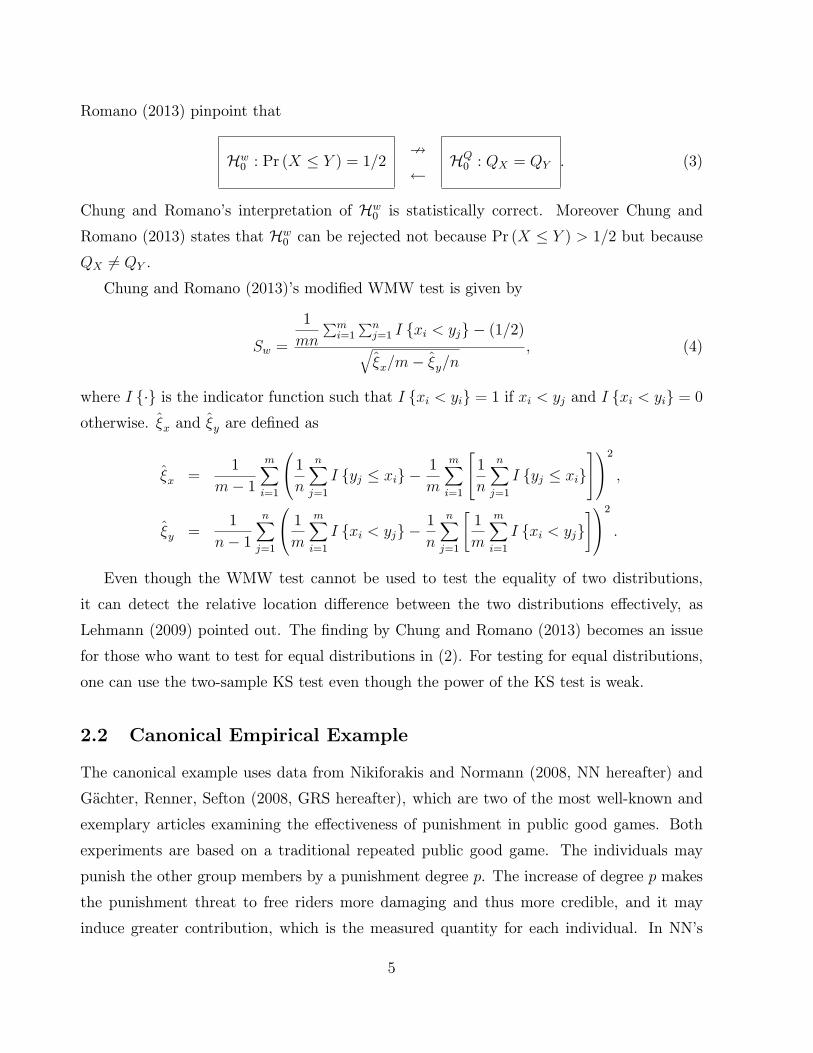
Romano (2013) pinpoint that

Hw0 : Pr (X � Y ) = 1=29

HQ0 : QX = QY : (3)

Chung and Romano's interpretation of Hw0 is statistically correct. Moreover Chung andRomano (2013) states that Hw0 can be rejected not because Pr (X � Y ) > 1=2 but becauseQX 6= QY :Chung and Romano (2013)'s modi�ed WMW test is given by

Sw =

1

mn

Pmi=1

Pnj=1 I fxi < yjg � (1=2)q�x=m� �y=n

; (4)

where I f�g is the indicator function such that I fxi < yig = 1 if xi < yj and I fxi < yig = 0otherwise. �x and �y are de�ned as

�x =1

m� 1

mXi=1

0@ 1n

nXj=1

I fyj � xig �1

m

mXi=1

24 1n

nXj=1

I fyj � xig351A2 ;

�y =1

n� 1

nXj=1

0@ 1m

mXi=1

I fxi < yjg �1

n

nXj=1

"1

m

mXi=1

I fxi < yjg#1A2 :

Even though the WMW test cannot be used to test the equality of two distributions,

it can detect the relative location di�erence between the two distributions e�ectively, as

Lehmann (2009) pointed out. The �nding by Chung and Romano (2013) becomes an issue

for those who want to test for equal distributions in (2). For testing for equal distributions,

one can use the two-sample KS test even though the power of the KS test is weak.

2.2 Canonical Empirical Example

The canonical example uses data from Nikiforakis and Normann (2008, NN hereafter) and

G�achter, Renner, Sefton (2008, GRS hereafter), which are two of the most well-known and

exemplary articles examining the e�ectiveness of punishment in public good games. Both

experiments are based on a traditional repeated public good game. The individuals may

punish the other group members by a punishment degree p. The increase of degree p makes

the punishment threat to free riders more damaging and thus more credible, and it may

induce greater contribution, which is the measured quantity for each individual. In NN's

5

study, p varies on a scale from 0 to 4 (the corresponding experiments are denoted as p0, p1,

p2, p3, p4), where 0 means there's no punishment opportunity in the game. There are 24

individuals in each of these �ve experiments. In GRS's design, there are four experiments

with di�erent p and di�erent numbers of rounds. For consistency, we only included the two

experiments with the same number of rounds (10) as in NN's, and we use p0 and p3 to

denote these. Here, p0 has 60 individuals, and p3 has 45. One important goal of NN's and

GRS's experiments is to test if the increase of p has an impact on overall contribution.

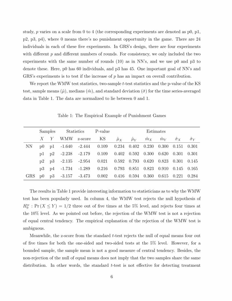
We report the WMW test statistics, two-sample t-test statistics and the p-value of the KS

test, sample means (�), medians (m), and standard deviation (�) for the time series-averaged

data in Table 1. The data are normalized to lie between 0 and 1.

Table 1: The Empirical Example of Punishment Games

Samples Statistics P-value Estimates

X Y WMW z-score KS �X �Y mX mY �X �Y

NN p0 p1 -1.640 -2.444 0.109 0.234 0.402 0.230 0.300 0.151 0.301

p1 p2 -2.238 -2.179 0.109 0.402 0.592 0.300 0.620 0.301 0.301

p2 p3 -2.135 -2.954 0.021 0.592 0.793 0.620 0.823 0.301 0.145

p3 p4 -1.734 -1.289 0.216 0.793 0.851 0.823 0.910 0.145 0.165

GRS p0 p3 -3.157 -3.473 0.002 0.416 0.594 0.360 0.615 0.221 0.284

The results in Table 1 provide interesting information to statisticians as to why the WMW

test has been popularly used. In column 4, the WMW test rejects the null hypothesis of

Hw0 : Pr (X � Y ) = 1=2 three out of �ve times at the 5% level, and rejects four times at

the 10% level. As we pointed out before, the rejection of the WMW test is not a rejection

of equal central tendency. The empirical explanation of the rejection of the WMW test is

ambiguous.

Meanwhile, the z-score from the standard t-test rejects the null of equal means four out

of �ve times for both the one-sided and two-sided tests at the 5% level. However, for a

bounded sample, the sample mean is not a good measure of central tendency. Besides, the

non-rejection of the null of equal means does not imply that the two samples share the same

distribution. In other words, the standard t-test is not e�ective for detecting treatment

6

e�ects in the second-order or higher -order.

The sixth column shows the p-value of the KS test, where the null hypothesis is distribu-

tional equality. Surprisingly the KS test only rejects the null hypothesis two out of �ve times

even at the 10% signi�cance level. Even when the sample means are signi�cantly di�erent,

the KS test does not reject the null that the distributions are the same. In other words, the

power of the KS test is very weak. That's why the KS test is not used very often in practice.

3 Practical Comparison of Two Samples

As demonstrated above, the power of the KS test is relatively weak. There are variants of

the KS test such as those by Cram�er-von Mises, Watson (1961) and Kuiper (1960) tests.

However, all these variants are based on the comparison of the two cumulative distribution

functions. If the two probability density functions (PDF) are the same, naturally the CDFs

are also the same. Two-sample comparisons based on equal PDFs are statistically elegant

but lack power. Here, we consider somewhat di�erent statistical testing procedures.

3.1 Comparison of Moments

It is well-known that if two CDFs are the same, then all of the moments of the two samples

must be identical. The opposite is true also as long as all moments exist and are �nite.

When the data are bounded this condition is clearly met, so it is possible to construct more

powerful tests using the moments. Denote �ik as the ith central moment of the kth sample

for i > 1 and �k as the �rst noncentral moment. Then the null Hm0 becomes identical to HQ0

as long as �ik exists.

Hm0 : �iX = �iY for all i () HQ0 : QX = QY

Of course, testing Hm0 is not feasible at all. Instead, we suggest testing a subset of Hm0 : Thatis, we are interested in testing the following subsets of Hm0 :

H�0 : �iX = �iY for all i � �:

When � = 1; the null of H�0 becomes the null of the z-score test, Hz0: When � = 3; the nullof H�0 implies that the two samples share the same mean, variance and skewness. If thenull hypothesis with � moments is rejected, then the treated sample di�ers from the control

7

sample `up to the �th-order.' For example, if the null with � = 2 is rejected; we say it that

there is a treatment e�ect up to the second-order.

This `subset approach' is convenient but at the same time raises an important question:

How should one choose a small value of �? Of course, �rst, the answer depends on the research

question. For example, if applied researchers care about the location of the distribution,

then they should choose � = 2 rather than � = 1. There are di�erent measures of statistical

location: mean, median, mode and quantile mean. However, it is not rare to see that the

median of X is greater than the median of Y even when the mean of X is smaller than the

mean of Y: When the two distributions are not symmetric, any such disagreement between

di�erences in means and medians becomes an issue. In this case, the skewness becomes

useful. Let mk be the median of the kth variable. Then, Pearson's nonparametric skewness

is de�ned as

Sk;non = 3�k �mkp�2k

;

where �k is the �rst noncentral moment. Since the median can be thought of as the weighted

mean, the nonparametric skewness can be thought of as a function of the �rst and second

moments. We will show later that this test with � = 2 becomes much more powerful than

the KS test.

The test statistic with � = 2 is straightforward. The following statistic has the limiting

distribution of �2 with 2 degrees of freedom as n and m!1

M2 = [�X � �Y ; �2X � �2Y ]��X=m+ �Y =n

��1[�X � �Y ; �2X � �2Y ]

0 !d �22; (5)

where

�k =

24 �2k �3k

�3k �4k � (�2k)2

35 ; for k = X; Y;and the circum ex indicates a sample average. If the two samples are dependent, then the

covariance matrix should be included in the inverse matrix, which is also straightforward.

See Appendix B for the proof.

However, there are two problems of the use ofM2: The �rst problem is a purely statistical

issue. The asymptotic result in (5) holds well only with large n and m: In fact, even when

QX and QY are truncated normal distributions, the exact distribution of M2 is unknown.

Second, even though the subset approach may detect distributional di�erences, this approach

is not particularly helpful in understanding changes in the shapes of the distributions across

8

di�erent treatments, which is important to theoreticians. To overcome this issue, we consider

the following alternative approach.

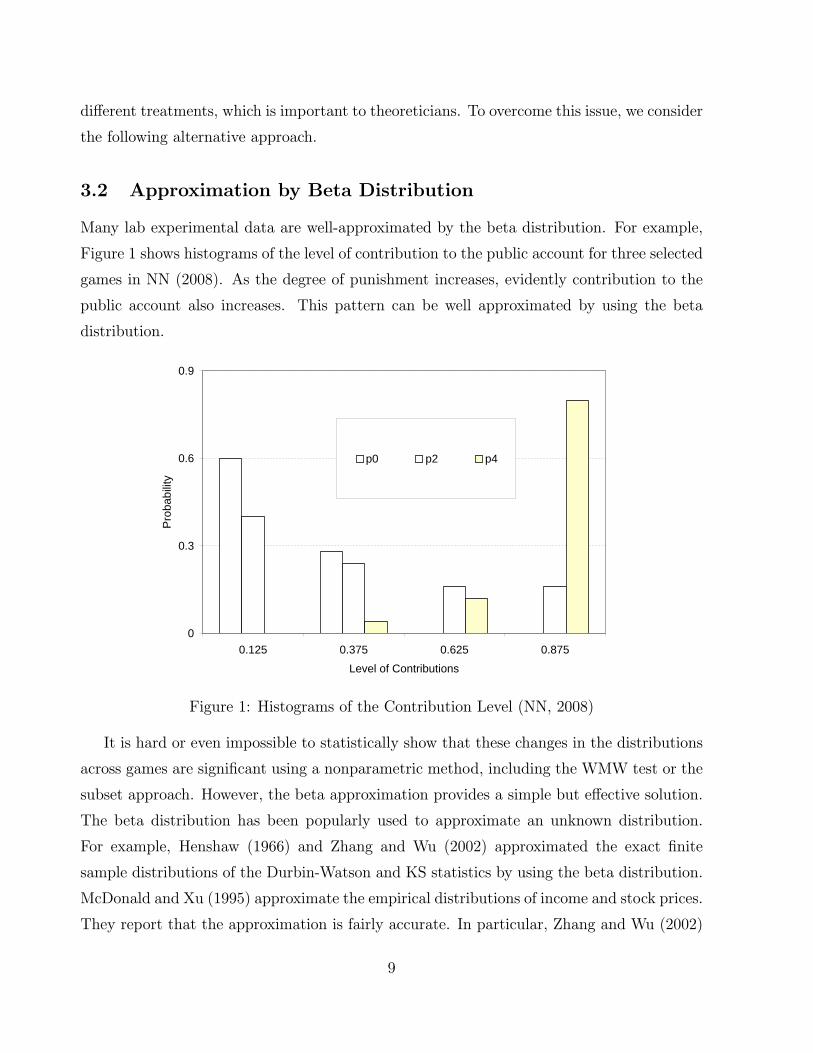
3.2 Approximation by Beta Distribution

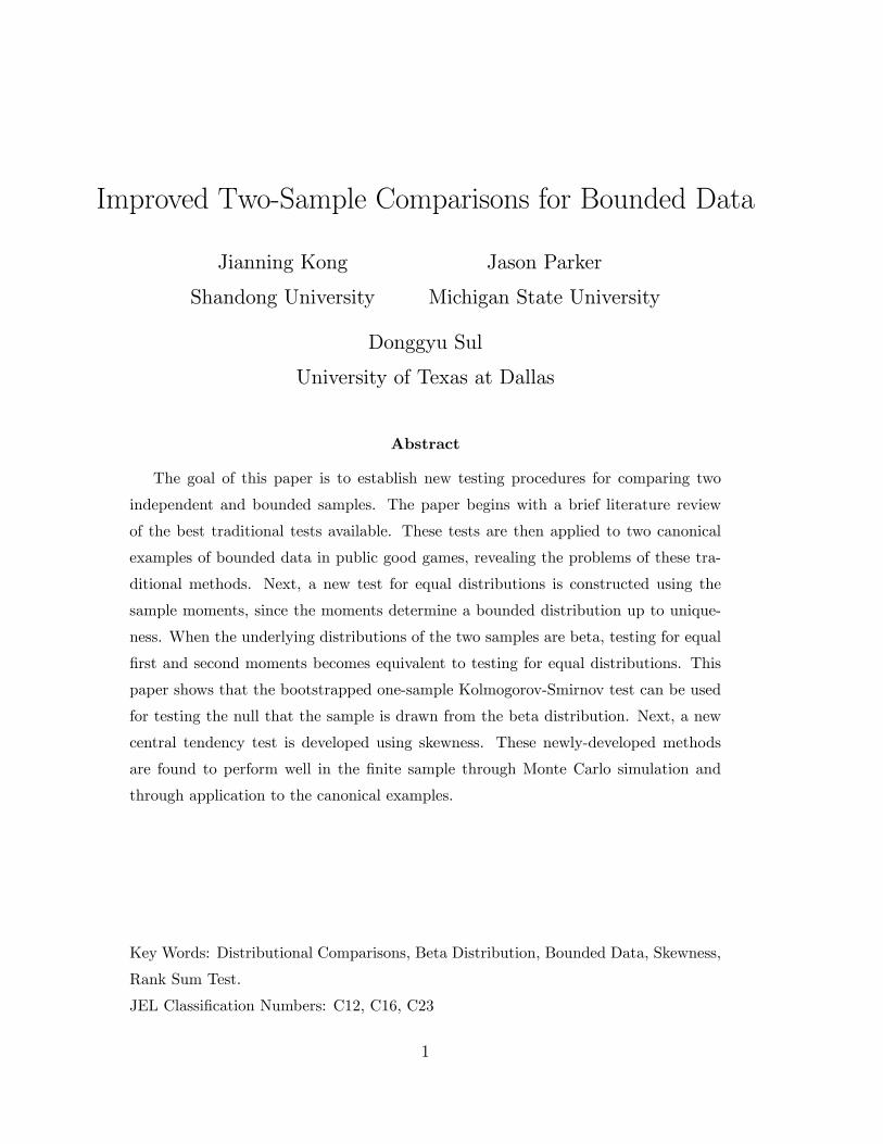
Many lab experimental data are well-approximated by the beta distribution. For example,

Figure 1 shows histograms of the level of contribution to the public account for three selected

games in NN (2008). As the degree of punishment increases, evidently contribution to the

public account also increases. This pattern can be well approximated by using the beta

distribution.

0

0.3

0.6

0.9

0.125 0.375 0.625 0.875Level of Contributions

Pro

babi

lity

p0 p2 p4

Figure 1: Histograms of the Contribution Level (NN, 2008)

It is hard or even impossible to statistically show that these changes in the distributions

across games are signi�cant using a nonparametric method, including the WMW test or the

subset approach. However, the beta approximation provides a simple but e�ective solution.

The beta distribution has been popularly used to approximate an unknown distribution.

For example, Henshaw (1966) and Zhang and Wu (2002) approximated the exact �nite

sample distributions of the Durbin-Watson and KS statistics by using the beta distribution.

McDonald and Xu (1995) approximate the empirical distributions of income and stock prices.

They report that the approximation is fairly accurate. In particular, Zhang and Wu (2002)

9

report that the beta approximation error is around the fourth digit di�erence even with a

small sample size. McDonald and Xu (1995) report in detail how many distributions can be

generated from the generalized beta distribution. See Figure 2 in McDonald and Xu (1995)

for a detailed explanation. Such exibility attracts many theoretical researchers to using

the beta distribution in their studies. Among many examples, here we list a few references

related to experimental studies: King and Lukas (1973), McKelvey and Palfrey (1992) and

Nyarko, Schotter and Sopher (2006).

Beta random variables are bounded between zero and one. The density can be convex or

concave. It can have a U-shape, L-shape or bell-shape, and it can be unimodal or bimodal.

The density function is given by

f (xj�; �) = 1

B (�; �)x��1 (1� x)��1 ; for x 2 [0; 1] ; � > 0; � > 0;

where B (�; �) =R 10 x

��1 (1� x)��1 dx; which is the beta function. This beta distributionhas many interesting properties which will be discussed below.

3.2.1 Null Spaces under the Beta Distribution

All moments including the median can be expressed as functions of � and �: For exam-

ple, �X = E (x) = �X= (�X + �X) ; �2X = V (x) = �X�Xh(�X + �X)

2 (�X + �X + 1)i�1

:

Hence, when the two samples share the same � and � values, the two samples come from the

same beta distribution. That is, the null hypothesis of equal distributions can be rewritten

as

HQ0 : �X = �Y & �X = �Y () HQ0 : QX = QY : (6)

Since the beta distribution can be characterized with only two parameters, � and �; the null

of equal distributions can also be expressed as

H�0 : �X = �Y & �2X = �2Y with � = 2 () HQ0 : QX = QY : (7)

That is, if the �rst two central moments of the two samples are the same, then the PDFs of

the two samples are identical.

Next, the standard z-score test is commonly used for the null hypothesis of equal means.

From simple and direct calculation, it is clear that

Hz0 : �X=�X = �Y =�Y () Hz0 : �X = �Y ; (8)

10

since equal means implies that �X= (�X + �X) = �Y = (�Y + �Y ) :

It is important to note that comparing means is not the only way to measure changes in

the locations of distributions.

3.2.2 Location Shift and Skewness under the Beta Distribution

Consider three location parameters: the mean, median and mode. Usually the location of a

distribution shifts to the right or left if one of these location parameter shifts right or left.

When a distribution is symmetric, all three measures are identical, so a change in one location

parameter implies a corresponding shift in the distribution. However, when a distribution

is not symmetric, it is not always the case that all three location parameters move in the

same direction. Under such a circumstance, it is very ambiguous to judge whether or not a

distribution has changed location.

As we discussed before, the notion of skewness is useful when the distribution is bounded.

Broadly, there are three di�erent measures of skewness:

Moments �3= (�2)3=2

Nonparametric 3 (��m) =p�2Quantile [F (u) + F (1� u)� 2F (0:5)] = [F (u)� F (1� u)]

where u stands for the arbitrary quantile. Under the beta distribution, the skewness based

on the moments has a one-for-one relationship with the nonparametric skewness and has

a positive relationship overall with the quantile skewness. Accordingly and without loss

of generality, we choose to use the de�nition of skewness based on the moments in this

paper, and denote it as S: By de�nition, the skewness is measuring where the mass of the

distribution is concentrated relative to the mean. If the skewness is positive (negative), the

mass of the distribution is located on the right (left) side of the mean. Hence, when the

distribution is bounded between zero and one, the notion of the skewness can be used as a

measure of the location of the distribution. It is important to note that the skewness cannot

be one of the location parameters when the distribution is unbounded. For example, under

the beta distribution, the skewness can be rewritten as a function of the mean and variance.

That is,

S =2 (1� 2�)�� (1� �) + �2 :

11

It is easy to show that with a �xed variance, the skewness has a one-for-one relationship

with the mean. That is,

@S

@�= �2� (2�

2 + 2�2 � 2�+ 1)(�2 � �2 + �)2

< 0 for 0 < � < 1; (9)

since �2 < � (1� �) by the Bhatia-Davis inequality. The inequality in (9) implies that theskewness decreases as the mean increases. In other words, the mass of the distribution moves

to the right.

Next, with a �xed mean, as the variance increases, the skewness changes also.

@S

@�= 2

(2�� 1) (�2 + �2 � �)(�2 � �2 + �)2

=

8<: > 0 if � < 0:5

< 0 if � > 0:5: (10)

The inequality in (10) states that with a �xed mean, as the variance increases, the mass of

the distribution moves to the left if S > 0 or the right if S < 0:

Note that the relationship between the median and the skewness is very similar but

the formulas are somewhat complicated, so they are omitted here. We have veri�ed their

relationship using direct calculation. That is, the skewness has a one-for-one relationship

with the median when the variance is �xed.

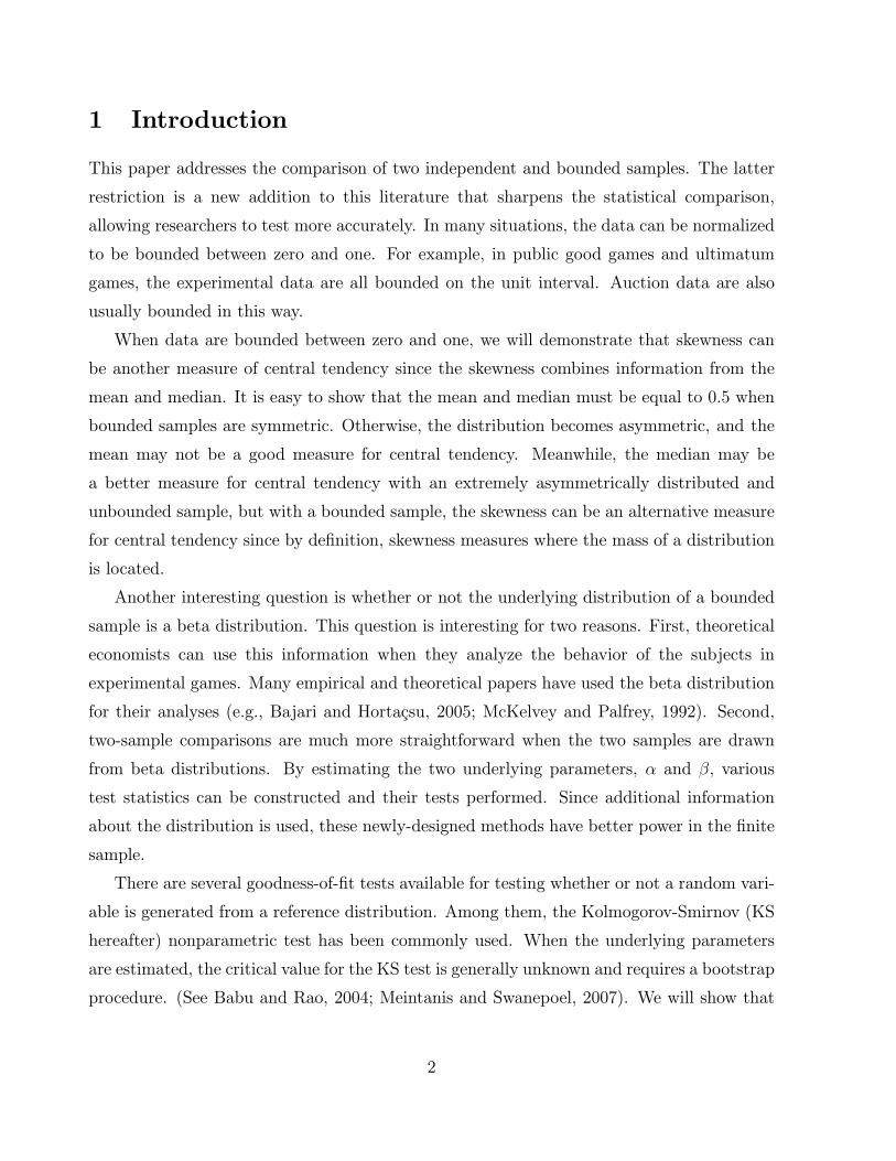
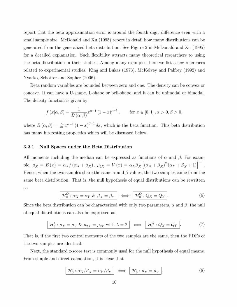
Some illustrations follow. For example, consider the following case where �X = 2; �X = 4;

�Y = 3; and �Y = 6: Both samples share the same mean of 0.33 but don't share either the

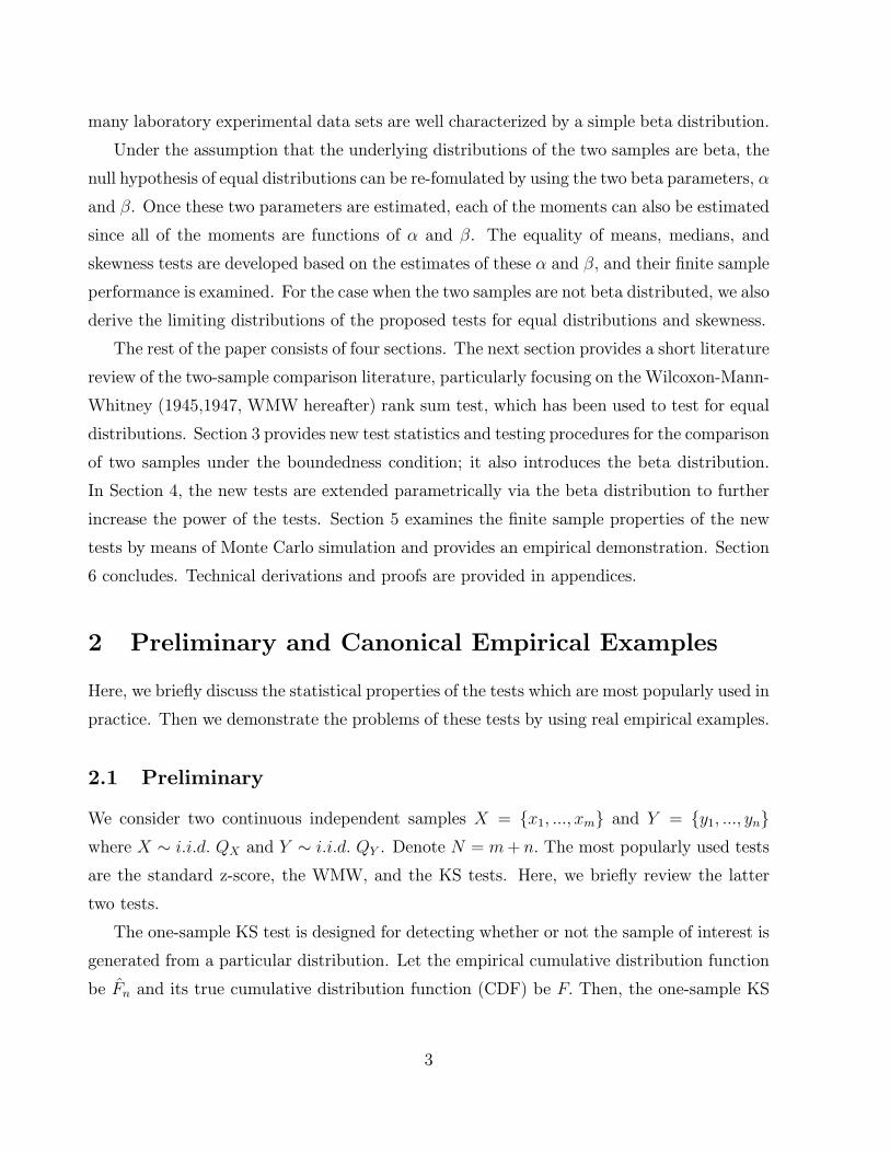
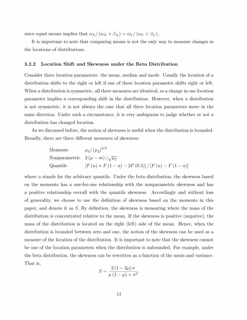
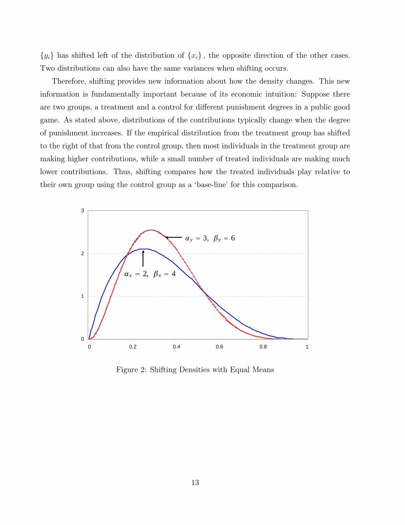
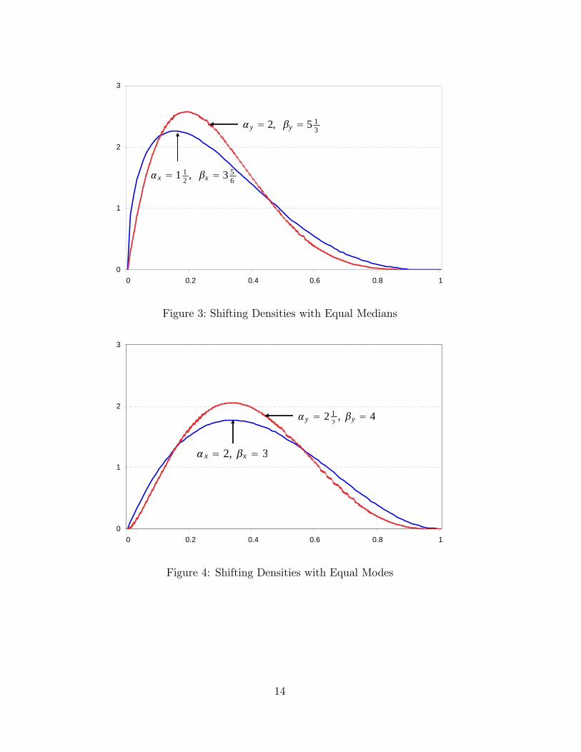
same variance or skewness. The skewness for fyig becomes 0.41 but that for fxig is 0.47.Hence the series fyig is less right skewed compared to the series fxig : Therefore, the mass ofthe empirical distribution of fyig shifts to the right of that of fxig : Figure 2 shows this caseexplicitly. Another example is where �X = 1:5; �X = 3:833; �Y = 2; and �Y = 5:333: Here,

both samples have the same median of 0.25 but the skewness, mean, and variance are all

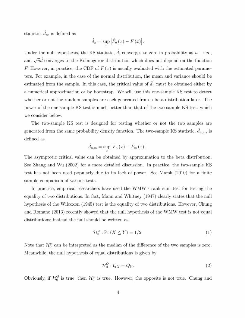
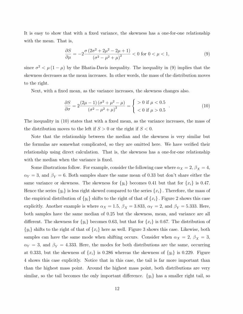
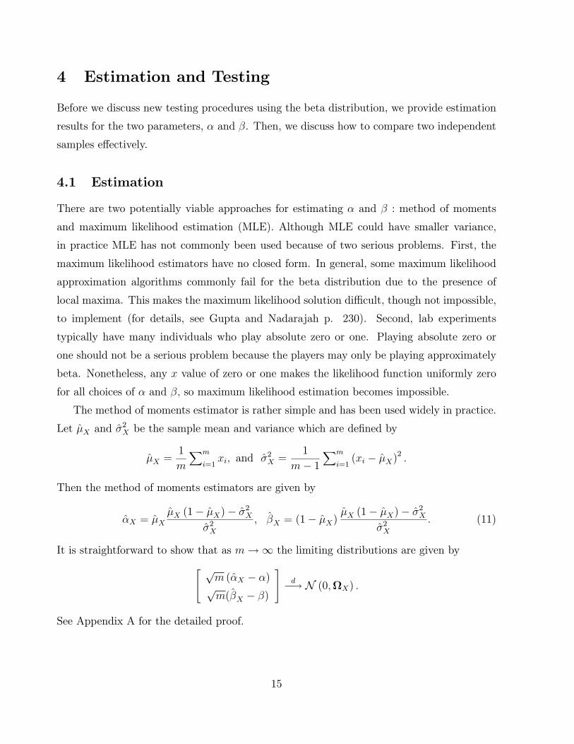
di�erent. The skewness for fyig becomes 0.63, but that for fxig is 0.67. The distribution offyig shifts to the right of that of fxig here as well. Figure 3 shows this case. Likewise, bothsamples can have the same mode when shifting occurs. Consider when �X = 2; �X = 3;

�Y = 3; and �Y = 4:333: Here, the modes for both distributions are the same, occurring

at 0.333, but the skewness of fxig is 0:286 whereas the skewness of fyig is 0:229. Figure4 shows this case explicitly. Notice that in this case, the tail is far more important than

than the highest mass point. Around the highest mass point, both distributions are very

similar, so the tail becomes the only important di�erence. fyig has a smaller right tail, so

12

fyig has shifted left of the distribution of fxig ; the opposite direction of the other cases.Two distributions can also have the same variances when shifting occurs.

Therefore, shifting provides new information about how the density changes. This new

information is fundamentally important because of its economic intuition: Suppose there

are two groups, a treatment and a control for di�erent punishment degrees in a public good

game. As stated above, distributions of the contributions typically change when the degree

of punishment increases. If the empirical distribution from the treatment group has shifted

to the right of that from the control group, then most individuals in the treatment group are

making higher contributions, while a small number of treated individuals are making much

lower contributions. Thus, shifting compares how the treated individuals play relative to

their own group using the control group as a `base-line' for this comparison.

0

1

2

3

0 0.2 0.4 0.6 0.8 1

Jx = 2, Kx = 4

Jy = 3, Ky = 6

Figure 2: Shifting Densities with Equal Means

13

0

1

2

3

0 0.2 0.4 0.6 0.8 1

Jx = 1 12 , Kx = 3 5

6

Jy = 2, Ky = 5 13

Figure 3: Shifting Densities with Equal Medians

0

1

2

3

0 0.2 0.4 0.6 0.8 1

J x = 2, Kx = 3

Jy = 2 12

, Ky = 4

Figure 4: Shifting Densities with Equal Modes

14

4 Estimation and Testing

Before we discuss new testing procedures using the beta distribution, we provide estimation

results for the two parameters, � and �. Then, we discuss how to compare two independent

samples e�ectively.

4.1 Estimation

There are two potentially viable approaches for estimating � and � : method of moments

and maximum likelihood estimation (MLE). Although MLE could have smaller variance,

in practice MLE has not commonly been used because of two serious problems. First, the

maximum likelihood estimators have no closed form. In general, some maximum likelihood

approximation algorithms commonly fail for the beta distribution due to the presence of

local maxima. This makes the maximum likelihood solution di�cult, though not impossible,

to implement (for details, see Gupta and Nadarajah p. 230). Second, lab experiments

typically have many individuals who play absolute zero or one. Playing absolute zero or

one should not be a serious problem because the players may only be playing approximately

beta. Nonetheless, any x value of zero or one makes the likelihood function uniformly zero

for all choices of � and �; so maximum likelihood estimation becomes impossible.

The method of moments estimator is rather simple and has been used widely in practice.

Let �X and �2X be the sample mean and variance which are de�ned by

�X =1

m

Xm

i=1xi; and �2X =

1

m� 1Xm

i=1(xi � �X)

2 :

Then the method of moments estimators are given by

�X = �X�X (1� �X)� �2X

�2X; �X = (1� �X)

�X (1� �X)� �2X�2X

: (11)

It is straightforward to show that as m!1 the limiting distributions are given by24 pm (�X � �)pm(�X � �)

35 d�! N (0;X) :

See Appendix A for the detailed proof.

15

4.2 Testing Procedures

Here we explain a two-step procedure detailing how to compare two independent samples,

and provide an asymptotic analysis of the proposed tests. The �rst null hypothesis to test

is the null of equal distributions, which is a pre-test for the location change test. If the two

samples share the same distribution, the second null hypothesis of the location change is not

needed. The null hypothesis of equal distributions is given in (6), and the test statistic B isde�ned as

B =h�X � �Y ; �X � �Y

i �x=m+ y=n

��1 h�X � �Y ; �X � �Y

i0;

where x is provided in Appendix A. The following theorem reveals the asymptotic properties

of this method.

Theorem 1 (Limiting Distribution of the B statistic) Assume that x1; : : : ; xm � iidBeta (�X ; �X), y1; : : : ; yn � iid Beta (�Y ; �Y ), and (xi; yj) are independent of each other forall i and j: Then, under HQ0 given in (6),

B d�! �22;

as n;m!1:

Theorem 1 is proved in Appendix A and shows that the equal distributions test is consistent

as n;m!1: Usually the 20% signi�cance level is used for pre-testing. In other words, we

recommend using 3.22 as the critical value for the beta distribution statistic B, which is the20% signi�cance level for the �22 distribution.

The next null hypothesis is location change. As we discussed earlier, the null of equal

locations is given by

HS0 : SX = SY : (12)

The null hypothesis of equal locations or equal skewness can be tested by using the method

of moments or Pearson's skewness test. However as we will show, the power of the test

of Pearson's skewness test is much worse than the power of the test based on the beta

distribution. The test statistic based on the beta distribution is given by

zSkew =S(Beta)X � S(Beta)Y

(J0XXJX=m+ J0YY JY =n)1=2;

16

where

Jk =

��k + �k

���k + �k + 2

�2q�k�k

q�k + �k + 1

�24�

��k + 1

� �3�k + �k + 2

��k

;(�k + 1)

��k + 3�k + 2

��k

350 ;and

S(Beta)k =

2��k � �k

�q�k + �k + 1q

�k�k��k + �k + 2

� for k = X;Y:

The following theorem shows the asymptotic performance of this estimator.

Theorem 2 (Limiting Distribution of the Skewness Statistic) Assume that x1; : : : ; xm

� iid Beta (�X ; �X), y1; : : : ; yn � iid Beta (�Y ; �Y ), and (xi; yj) are independent of eachother for all i and j: Then, under HS0 given in (12),

zSkewd�! N (0; 1) ;

as n;m!1.

Theorem 2 is proved in Appendix A and shows that the equal skewness test is consistent as

n;m!1:So far, we have assumed that the two samples are independent. Hence all the test

statistics considered in this paper are valid only under this independence assumption. In

public good games, it is well-known that the contribution levels for each subject are correlated

over rounds. In other words, the proposed tests cannot be performed for the comparison of

a pair of two samples across rounds due to serial dependence. However, theoretically this

restriction can be relaxed by accounting for a dependence structure. In order to analyze

paired data (x1; y1) ; : : : ; (xn; yn) using the beta approach, a bivariate beta distribution must

be assumed. This distribution is still an active area of research. Some of these distributions

will lend themselves to this estimation better than others. For instance, El-Bassiouny and

Jones (2005) provide a distribution which nests many other bivariate beta distributions, with

joint density:

f (x; y) = Cxa=2�1 (1� x)(b+d)=2�1 yb=2�1 (1� y)(a+d)=2�1

(1� xy)(a+b)=2F

a+ b

2;d� c2;a+ d

2;x (1� y)1� xy

!;

17

where C is a constant de�ned so that the double integral equals unity and 0 < x; y < 1. The

moments of this distribution involve the generalized hypergeometric function, so the method

of moments estimator will not have a closed form. Similarly, the �ve parameter bivariate

beta distribution in Gupta and Wong (1985) has moments which involve the generalized hy-

pergeometric function. Other choices include the three parameter bivariate beta distribution

from Gupta and Wong (1985) with joint density:

f (x; y) =� (a+ b+ c)

� (a) � (b) � (c)xa�1yb�1 (1� x� y)c�1 ;

where x+ y � 1 and x; y > 0 and where � (x) is the gamma function. Because this densityhas only three parameters and because the inequality is restrictive, this density is not very

general. Nadarajah and Kotz (2005) de�ne the density

f (x; y) =xc�1 (y � x)b�1 ya1�c�b (1� y)b1�1

B (a1; b1)B (c; b)

where 0 � x � y � 1. Because of the inequality, this distribution is also quite restrictive. Ifa general bivariate beta distribution with closed-form method of moments estimators cannot

be developed, then approximation methods can be used with some existing bivariate beta

distributions.

As we discussed earlier and will show shortly, the bootstrap one-sample KS test can be

used for testing whether or not a random variable follows the beta distribution. Since this

bootstrap one-sample KS test can be considered a pre-test, the 20% signi�cance level should

be used. However, either when the bootstrap one-sample KS test rejects the null of the beta

distribution or when the two samples are not independent, the following moments test can

be used up to � = 2: The major drawback of this moment-based test, however, is that the

rejection of the null hypothesis H�0 in (7) implies the rejection of the equal distributions butthe opposite does not hold. The moments test statistic for the equal distributions test is

B� = nh�x� �y; �2x � �2y

i��1

h�x� �y; �2x � �2y

i0where � is de�ned in Appendix B. Under the null of equal distributions, B� converges indistribution to the �22-distribution as n!1, which follows from Lemma 5 in Appendix B.

The moments test statistic for the equal skewness test is

z�Skew =pn

SX � SYq!X + !Y � 2!X;Y

18

where !X ; !Y ; and !X;Y are de�ned in Appendix B. Under the null of equal skewness, z�Skew

converges in distribution to the standard normal distribution as n!1, which follows fromLemma 4 in Appendix B.

In the following section, a testing procedure for whether or not the samples follow beta

distributions is proposed and the �nite sample performance of the moments tests is also

examined.

5 Monte Carlo Simulation and Empirical Example

This section consists of two subsections. The �rst subsection details the �nite sample perfor-

mance of the one-sample bootstrapped KS test, the WMW test, and the sequential testing

procedure. The second subsection demonstrates the e�ectiveness of the suggested test sta-

tistics.

5.1 Monte Carlo Simulation

The tests are performed at the 5% nominal level. For all cases except for the bootstrapped

one-sample KS test, 10,000 replications are used whereas for the cases of the bootstrapped

one-sample KS test, 2,000 replications are used and for each replication 1,000 bootstrap

replications are used. We use the following bootstrap procedure for the one-sample KS test.

Bootstrap Procedure for The One-Sample KS Test

Step 1: Estimate � and � by using the method of moments. Obtain the one-sample KS

statistic based on the estimated � and �:

Step 2: Generate n pseudo-beta random variables with � and �: Estimate � and � using

the pseudorandom variables. Obtain the one-sample KS statistic.1

Step 3: Repeat Step 2 for 1,000 times. Obtain the critical value from the bootstrapped

distribution and compare the KS statistic in Step 1 with this critical value. If the KS

statistic in Step 1 is larger than the bootstrapped critical value, the null of the beta

distribution is rejected.

1As Babu and Rao (2004) and Meintanis and Swanepoel (2009) point out, the above parametric bootstrap

procedure does not need to correct any bias in the method of moments estimation.

19

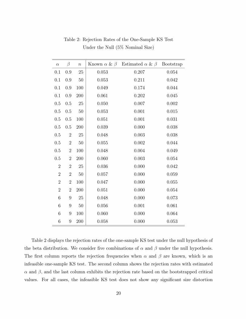
Table 2: Rejection Rates of the One-Sample KS Test

Under the Null (5% Nominal Size)

� � n Known � & � Estimated � & � Bootstrap

0.1 0.9 25 0.053 0.207 0.054

0.1 0.9 50 0.053 0.211 0.042

0.1 0.9 100 0.049 0.174 0.044

0.1 0.9 200 0.061 0.202 0.045

0.5 0.5 25 0.050 0.007 0.002

0.5 0.5 50 0.053 0.001 0.015

0.5 0.5 100 0.051 0.001 0.031

0.5 0.5 200 0.039 0.000 0.038

0.5 2 25 0.048 0.003 0.038

0.5 2 50 0.055 0.002 0.044

0.5 2 100 0.048 0.004 0.049

0.5 2 200 0.060 0.003 0.054

2 2 25 0.036 0.000 0.042

2 2 50 0.057 0.000 0.059

2 2 100 0.047 0.000 0.055

2 2 200 0.051 0.000 0.054

6 9 25 0.048 0.000 0.073

6 9 50 0.056 0.001 0.061

6 9 100 0.060 0.000 0.064

6 9 200 0.058 0.000 0.053

Table 2 displays the rejection rates of the one-sample KS test under the null hypothesis of

the beta distribution. We consider �ve combinations of � and � under the null hypothesis.

The �rst column reports the rejection frequencies when � and � are known, which is an

infeasible one-sample KS test. The second column shows the rejection rates with estimated

� and �; and the last column exhibits the rejection rate based on the bootstrapped critical

values. For all cases, the infeasible KS test does not show any signi�cant size distortion

20

even in small samples (n = 25). Meanwhile, as we discussed earlier, the one-sample KS test

using the estimates of � and � su�ers from serious size distortion. The direction of the size

distortion depends on the values of � and �:When � < � < 1; the one-sample KS test su�ers

from upward size distortion. Otherwise, the one-sample KS test su�ers from downward size

distortion. Once the bootstrap critical values are used, the size distortion is reduced in every

case, and as n increases, the rejection rates converge to the nominal size of 5%.

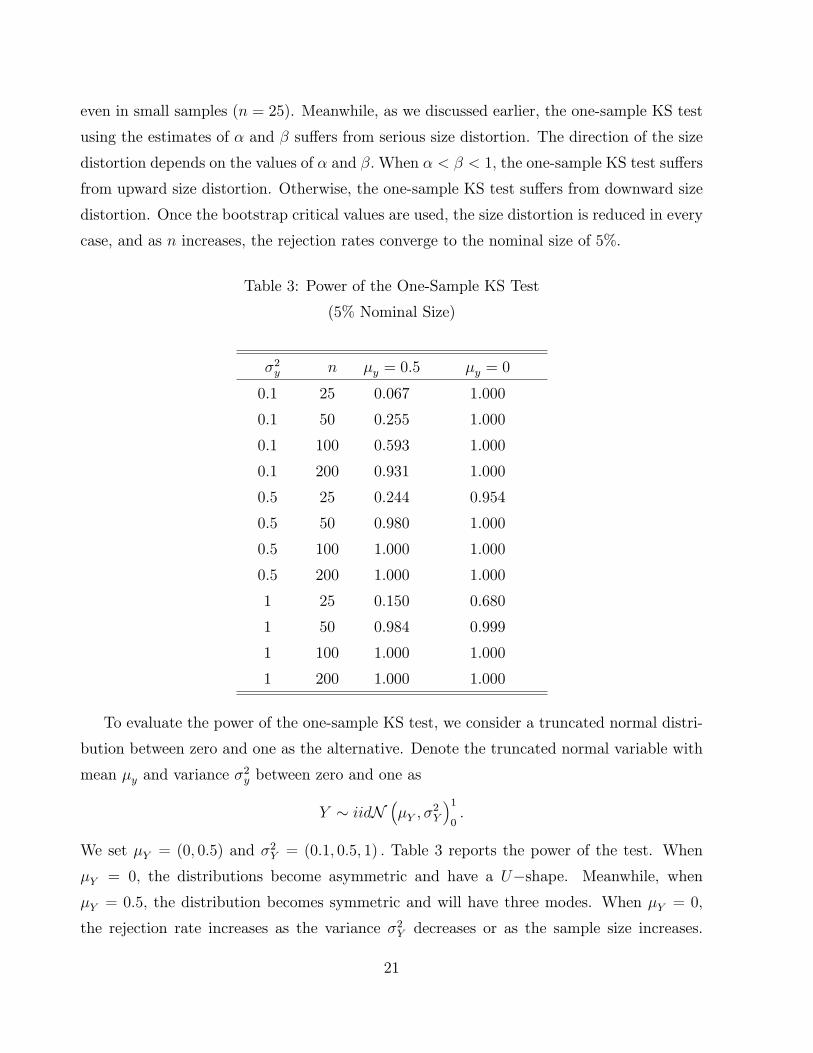
Table 3: Power of the One-Sample KS Test

(5% Nominal Size)

�2y n �y = 0:5 �y = 0

0.1 25 0.067 1.000

0.1 50 0.255 1.000

0.1 100 0.593 1.000

0.1 200 0.931 1.000

0.5 25 0.244 0.954

0.5 50 0.980 1.000

0.5 100 1.000 1.000

0.5 200 1.000 1.000

1 25 0.150 0.680

1 50 0.984 0.999

1 100 1.000 1.000

1 200 1.000 1.000

To evaluate the power of the one-sample KS test, we consider a truncated normal distri-

bution between zero and one as the alternative. Denote the truncated normal variable with

mean �y and variance �2y between zero and one as

Y � iidN��Y ; �

2Y

�10:

We set �Y = (0; 0:5) and �2Y = (0:1; 0:5; 1) : Table 3 reports the power of the test. When

�Y = 0; the distributions become asymmetric and have a U�shape. Meanwhile, when

�Y = 0:5; the distribution becomes symmetric and will have three modes. When �Y = 0;

the rejection rate increases as the variance �2Y decreases or as the sample size increases.

21

When �Y = 0:5; the rejection rate does not seem to depend much on the variance. However,

as n increases, the rejection rate approaches unity in all cases.

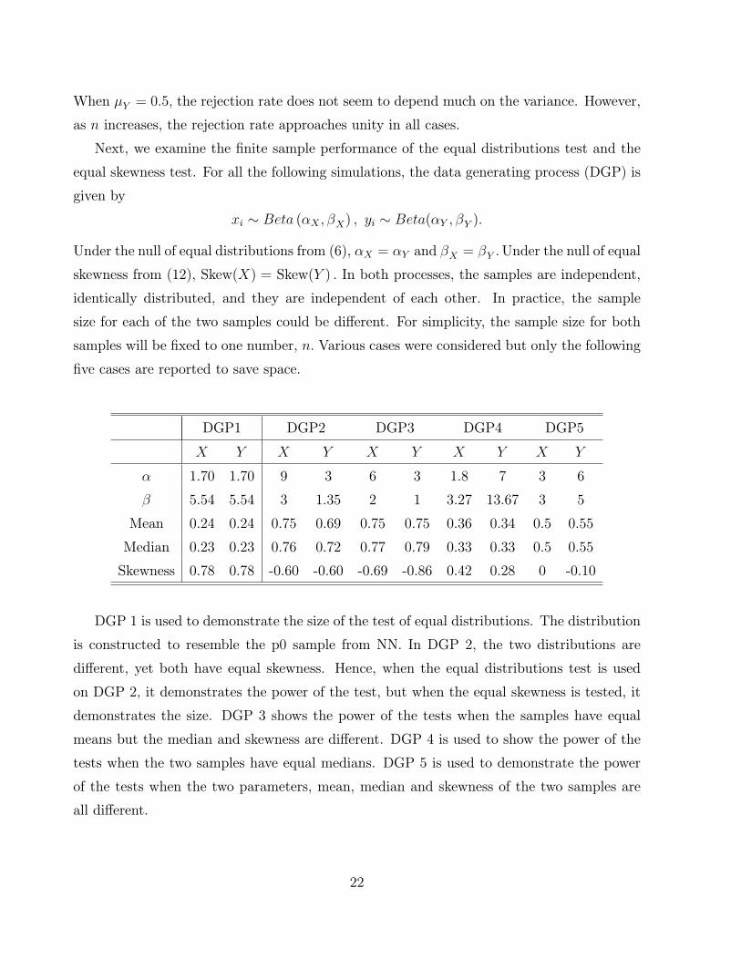
Next, we examine the �nite sample performance of the equal distributions test and the

equal skewness test. For all the following simulations, the data generating process (DGP) is

given by

xi � Beta (�X ; �X) ; yi � Beta(�Y ; �Y ):

Under the null of equal distributions from (6), �X = �Y and �X = �Y :Under the null of equal

skewness from (12), Skew(X) = Skew(Y ) : In both processes, the samples are independent,

identically distributed, and they are independent of each other. In practice, the sample

size for each of the two samples could be di�erent. For simplicity, the sample size for both

samples will be �xed to one number, n: Various cases were considered but only the following

�ve cases are reported to save space.

DGP1 DGP2 DGP3 DGP4 DGP5

X Y X Y X Y X Y X Y

� 1.70 1.70 9 3 6 3 1.8 7 3 6

� 5.54 5.54 3 1.35 2 1 3.27 13.67 3 5

Mean 0.24 0.24 0.75 0.69 0.75 0.75 0.36 0.34 0.5 0.55

Median 0.23 0.23 0.76 0.72 0.77 0.79 0.33 0.33 0.5 0.55

Skewness 0.78 0.78 -0.60 -0.60 -0.69 -0.86 0.42 0.28 0 -0.10

DGP 1 is used to demonstrate the size of the test of equal distributions. The distribution

is constructed to resemble the p0 sample from NN. In DGP 2, the two distributions are

di�erent, yet both have equal skewness. Hence, when the equal distributions test is used

on DGP 2, it demonstrates the power of the test, but when the equal skewness is tested, it

demonstrates the size. DGP 3 shows the power of the tests when the samples have equal

means but the median and skewness are di�erent. DGP 4 is used to show the power of the

tests when the two samples have equal medians. DGP 5 is used to demonstrate the power

of the tests when the two parameters, mean, median and skewness of the two samples are

all di�erent.

22

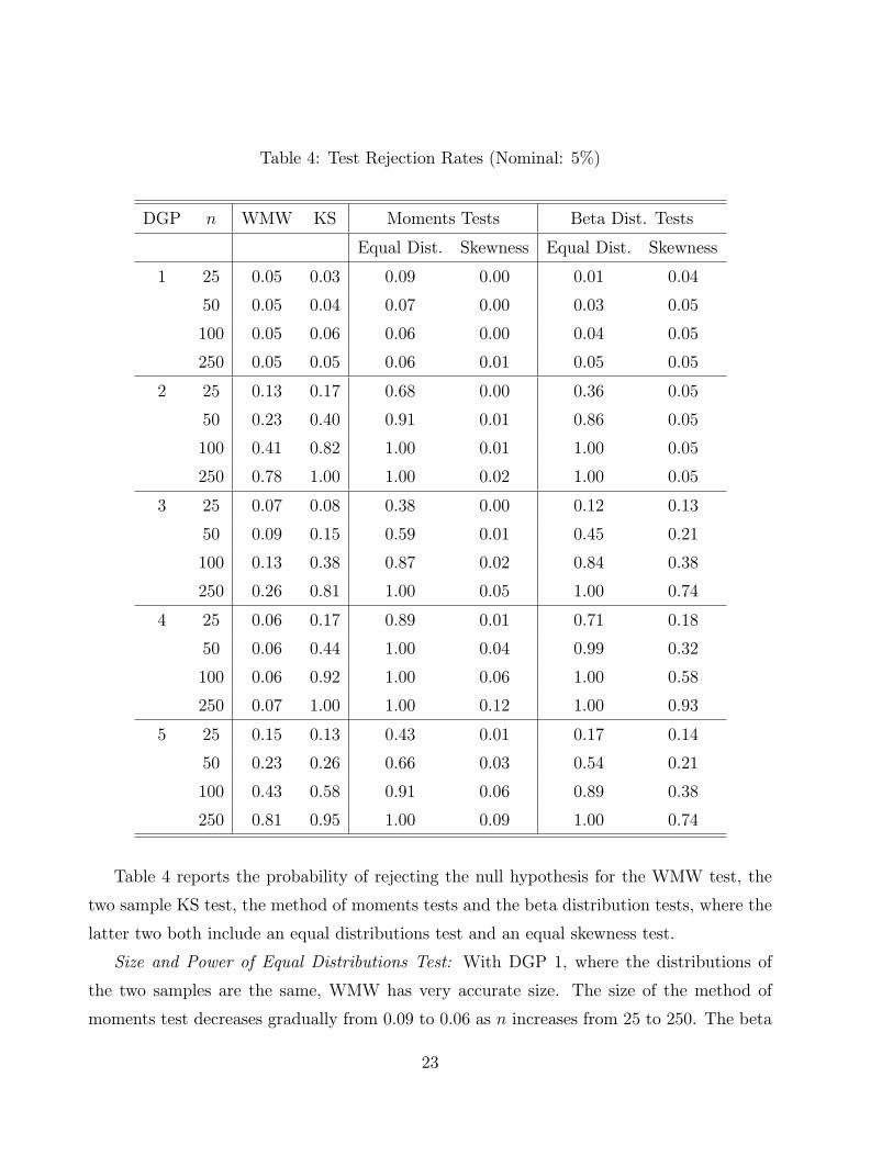
Table 4: Test Rejection Rates (Nominal: 5%)

DGP n WMW KS Moments Tests Beta Dist. Tests

Equal Dist. Skewness Equal Dist. Skewness

1 25 0.05 0.03 0.09 0.00 0.01 0.04

50 0.05 0.04 0.07 0.00 0.03 0.05

100 0.05 0.06 0.06 0.00 0.04 0.05

250 0.05 0.05 0.06 0.01 0.05 0.05

2 25 0.13 0.17 0.68 0.00 0.36 0.05

50 0.23 0.40 0.91 0.01 0.86 0.05

100 0.41 0.82 1.00 0.01 1.00 0.05

250 0.78 1.00 1.00 0.02 1.00 0.05

3 25 0.07 0.08 0.38 0.00 0.12 0.13

50 0.09 0.15 0.59 0.01 0.45 0.21

100 0.13 0.38 0.87 0.02 0.84 0.38

250 0.26 0.81 1.00 0.05 1.00 0.74

4 25 0.06 0.17 0.89 0.01 0.71 0.18

50 0.06 0.44 1.00 0.04 0.99 0.32

100 0.06 0.92 1.00 0.06 1.00 0.58

250 0.07 1.00 1.00 0.12 1.00 0.93

5 25 0.15 0.13 0.43 0.01 0.17 0.14

50 0.23 0.26 0.66 0.03 0.54 0.21

100 0.43 0.58 0.91 0.06 0.89 0.38

250 0.81 0.95 1.00 0.09 1.00 0.74

Table 4 reports the probability of rejecting the null hypothesis for the WMW test, the

two sample KS test, the method of moments tests and the beta distribution tests, where the

latter two both include an equal distributions test and an equal skewness test.

Size and Power of Equal Distributions Test: With DGP 1, where the distributions of

the two samples are the same, WMW has very accurate size. The size of the method of

moments test decreases gradually from 0.09 to 0.06 as n increases from 25 to 250. The beta

23

distribution test is mildly conservative when n is small, but the size becomes close to 0.05

when n is large. In terms of power of the test { as demonstrated using DGP 2 to DGP 5

{ both equal distributions tests substantially dominates the WMW and KS tests and both

reject perfectly when n is greater than 100. When the moments test and the beta distribution

test are compared, beta distribution test has lower power.

Size and Power of the Equal Skewness Test: Here, the distribution pre-test is performed

at the 20% level, while the other tests are performed at the 5% level. DGP 2 shows the size

of the equal skewness tests, while DGP 3 to DGP 5 demonstrate the power. In terms of

size, the beta distribution test is quite accurate even when n is small, whereas the method

of moments test shows undersize distortion, rejecting in less than 5% of cases. Also, the

equal skewness test using the beta distribution is quite powerful. With DGP 2 to DGP 5,

the power of the moments test is quite low even when n is large, while the power of the beta

distribution test increases quickly.

5.2 Return to the Empirical Examples

Here we demonstrate the e�ectiveness of the suggested tests. Before we estimate � and �, we

test whether or not each sample is drawn from the beta distribution. Using the bootstrapped

one-sample KS test, we cannot reject the null of the beta distribution for all seven samples

at the 5% level.

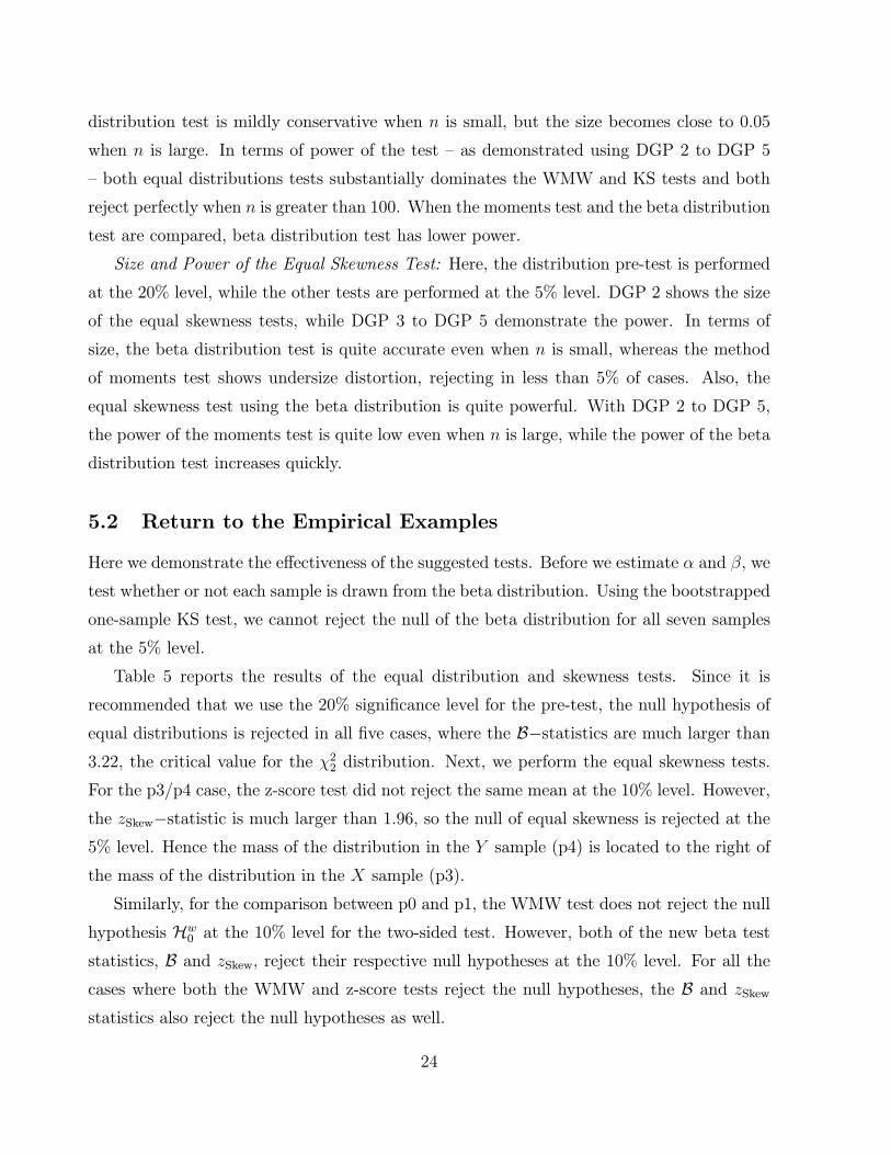
Table 5 reports the results of the equal distribution and skewness tests. Since it is

recommended that we use the 20% signi�cance level for the pre-test, the null hypothesis of

equal distributions is rejected in all �ve cases, where the B�statistics are much larger than3.22, the critical value for the �22 distribution. Next, we perform the equal skewness tests.

For the p3/p4 case, the z-score test did not reject the same mean at the 10% level. However,

the zSkew�statistic is much larger than 1.96, so the null of equal skewness is rejected at the5% level. Hence the mass of the distribution in the Y sample (p4) is located to the right of

the mass of the distribution in the X sample (p3).

Similarly, for the comparison between p0 and p1, the WMW test does not reject the null

hypothesis Hw0 at the 10% level for the two-sided test. However, both of the new beta test

statistics, B and zSkew; reject their respective null hypotheses at the 10% level. For all the

cases where both the WMW and z-score tests reject the null hypotheses, the B and zSkewstatistics also reject the null hypotheses as well.

24

Table 5: Canonical Examples Reexamined using the Beta Tests (Standard Errors)

X Y WMW z-score KS �X �X �Y �Y B zSkew

NN p0 p1 -1.640 -2.444 0.109 1.697 5.544 0.713 1.059 6.422 1.655

(0.51) (1.77) (0.21) (0.33)

p1 p2 -2.238 -2.179 0.109 0.713 1.059 1.052 0.726 3.796 2.159

(0.21) (0.33) (0.33) (0.22)

p2 p3 -2.135 -2.954 0.021 1.052 0.726 5.625 1.465 6.515 2.183

(0.33) (0.22) (1.85) (0.45)

p3 p4 -1.734 -1.289 0.216 5.625 1.465 3.264 0.570 3.852 1.992

(1.85) (0.45) (1.27) (0.20)

GRS p0 p3 -3.157 -3.473 0.002 1.683 2.360 1.225 0.838 13.390 3.325

(0.31) (0.44) (0.27) (0.18)

6 Conclusion

In this paper, we began by summarizing the literature on two-sample comparisons. In

particular, the WMW test, the traditional z-score test, and the KS test are the best at

testing the null hypotheses of zero median di�erence, equal means, and equal distributions,

respectively. We then used these three tests with two canonical examples of public good

games, �nding that the WMW and the z-score tests perform adequately, but that the KS

test has low power in the �nite sample.

Next, we devised two new approaches to the two-sample comparison problem, which are

then used to develop new tests. The �rst new approach concerns testing for equal distribu-

tions. In the context of bounded data, the moments completely determine a distribution up

to uniqueness, so it is possible to test for equal distributions by simply testing the moments.

The second new approach concerns testing for location changes in bounded data. Since the

mean, median, and mode are all free oating, it is somewhat common in bounded data that

one moves right and another left, making these common measures of central tendency inad-

equate. We �nd that changes in skewness robustly convey much of the information about

the overall movement of bounded densities. The derivations of these new tests are provided.

25

Afterward, we propose using the beta distribution to perform these tests parametrically

to �nd important estimation results and increase the power of the tests. Since an approxi-

mate beta distribution cannot always be assumed, we advocate using a one-sample KS test

for the beta distribution, which performs quite well in the �nite sample. The two parameters

for the beta distribution are estimated using the method of moments, because the maximum

likelihood estimator commonly does not exist for experimental data. The limiting distribu-

tion of the beta distribution parameter estimators is provided. Distributional testing follows

from knowing the limiting distribution of the parameter estimators, and the beta distribution

equal skewness test is also provided.

Finally, we evaluate the �nite sample performance of our newly developed methods

through Monte Carlo simulations and through application to the canonical examples. We

�nd that the new beta tests perform quite well in the �nite sample from the Monte Carlo

study. In the empirical example, for the tests of the null hypothesis that the samples are

drawn from the beta distribution, each of the seven cases accepts the null at the 5% level,

so it seems quite likely that the beta tests will perform reasonably well. In all �ve cases, we

�nd that the new distribution test rejects the null of equal distributions at the recommended

20% level. We also �nd that the new skewness test rejects the null in four of the �ve cases

at the 5% level.

26

References

[23] Babu, G. J. and C. R. Rao (2004): \Goodness-of-�t tests when parameters are esti-

mated." Sankhy�a, 66(1), 63-74.

[23] Bajari, P. and A. Horta�csu (2003): \Are structural estimates of auction models reason-

able? Evidence from experimental data." (No. w9889) National Bureau of Economic

Research.

[23] Chung, E. and J. P. Romano (2013): \Exact and asymptotically robust permutation

tests." Annals of Statistics, 41(2), 484-507.

[23] El-Bassiouny, A. H. and M. C. Jones (2009): \A bivariate F distribution with marginals

on arbitrary numerator and denominator degrees of freedom, and related bivariate beta

and t distributions." Statistical Methods and Applications, 18(4), 465-481.

[23] G�achter, S., Renner, E., and M. Sefton (2008): \The long-run bene�ts of punishment."

Science, 322(5907), 1510-1510.

[23] Gupta, A. K. and S. Nadarajah (2004): Handbook of the Beta Distribution and its

Applications. CRC Press.

[23] Gupta, A. K. and C. F. Wong (1985): \On three and �ve parameter bivariate beta

distributions." Metrika, 32(1), 85-91.

[23] Henshaw, R. C. Jr. (1966): \Testing single-equation least squares regression models for

autocorrelated disturbances." Econometrica, 34(3), 646-660.

[23] King, W. R. and P. A. Lukas (1973): \An experimental analysis of network planning."

Management Science, 19(12), 1423-1432.

[23] Kuiper, N. H. (1960): \Tests concerning random points on a circle." Proceedings of the

Koninklijke Nederlandse Akademie van Wetenschappen-Series A, 63, 38-47.

[23] MacGillivray, H. L. (1981): \The mean, median, mode inequality and skewness for a

class of densities." Australian Journal of Statistics, 23(2), 247-250.

27

[23] Mann, H. B. and D. R. Whitney (1947): \On a test of whether one of two random

variables is stochastically larger than the other." Annals of Mathematical Statistics,

18(1), 50-60.

[23] Marsh, P. (2010): \A two-sample nonparametric likelihood ratio test." Journal of Non-

parametric Statistics, 22(8), 1053-1065.

[23] McDonald, J. B. and Y. J. Xu (1995): \A generalization of the beta distribution with

applications." Journal of Econometrics, 66(1), 133-152.

[23] McKelvey, R. D. and T. R. Palfrey (1992): \An experimental study of the centipede

game." Econometrica, 60(4), 803-836.

[23] Meintanis, S. and J. Swanepoel (2007): \Bootstrap goodness-of-�t tests with estimated

parameters based on empirical transforms." Statistics and Probability Letters, 77(10),

1004-1013.

[23] Nadarajah, S. and S. Kotz (2005): \Some bivariate beta distributions." Statistics, 39(5),

457-466.

[23] Nadarajah, S. (2005): \Reliability for some bivariate beta distributions." Mathematical

Problems in Engineering, 2005(1), 101-111.

[23] Nikiforakis, N. and H. T. Normann (2008): \A comparative statics analysis of punish-

ment in public-good experiments." Experimental Economics, 11(4), 358-369.

[23] Nyarko, Y., A. Schotter, and B. Sopher (2006): \On the informational content of advice:

A theoretical and experimental study." Economic Theory, 29(2), 433-452.

[23] Watson, G. S. (1961): \Goodness-of-�t tests on a circle." Biometrika, 61(1/2), 109-114.

[23] Wilcoxon, F. (1945): \Individual comparisons by ranking methods." Biometrics Bul-

letin, 1(6), 80-83.

[23] Zhang, J. and Y. Wu (2002): \Beta approximation to the distribution of Kolmogorov-

Smirnov statistic." Annals of the Institute of Statistical Mathematics, 54(3), 577-584.

28

Appendix A { Proofs for Beta Tests

De�ne �k as the non-central moments of beta random variable x; which is given by

�k = Ehxki=

k�1Yi=0

�x + i

�x + �x + i:

Next, de�ne

x = Joo

xJo0;

where

Jo =

24 (�2 � �21)�1 0 � (�2 � �21)�2�1 (�1 � �2)

0 (�2 � �21)�1 � (�2 � �21)

�2(1� �1) (�1 � �2)

35 ;and

ox =

26664�11 �12 �13

�12 �22 �23

�13 �23 �33

37775 ;with

�11 = � 4 + 4 (�2 � �3)�21 � 4�1�22;

�12 = � 1 � � 4 � � 2 + 6�21�3 + (1 + 2�2)�1�2 � �22;

�13 = �� 1 � 2� 3 � 2 (1 + 2�1)�21�2 + 2�1�3;

�22 = 2� 1 + � 4 + 2� 2 � (1 + 4�2)�21 + (1 + �2)�2 � 2�3 + �4;

�23 = � 1 + 2� 3 + 2 (1 + 2�2)�31 + (3�2 � 5�1)�2 + �3 � �4;

�33 = 4�3�2 � �21

��21 � 4�1�3 � 5�22 + �4;

where � 1 = �1�4 + �2�3 � 2�3�21; � 2 = 3�1�3 + 2�31 � �1�2; � 3 = 3�21�2 � 3�1�22 � 2�41;

� 4 = �32�4�41 �4�21�22 +8�31�2+�21�4 +2�1�2�3: y is similarly de�ned as x so the formula

for y is omitted to save space.

For Lemma 1, we further de�ne ns = n� s; e.g. n1 = n� 1, and �xk = (n�1Pni=1 xi)

k:

Lemma 1 (Expected Values of Beta Family Sample Moments) If x1; : : : ; xn are

drawn from a random sample beta distribution, then the expectations of the following powers

29

are:

E [�x] = �1

nEh�x2i= n1�

21 + �2

n2Eh�x3i= n1n2�

31 + 3n1�1�2 + �3

n3Eh�x4i= n1n2n3�

41 + 6n1n2�

21�2 + n1

�3�22 + 4�1�3

�+ �4

Eh�s2x + �x

2�i

= �2

nEh�x�s2x + �x

2�i

= n1�1�2 + �3

n2Eh�x2�s2x + �x

2�i

= n1n2�21�2 + n1

�2�1�3 + �

22

�+ �4

n3Eh�x3�s2x + �x

2�i

= n1n2n3�31�2 + 3n1n2

��21�3 + �1�

22

�+ n1 (4�2�3 + 3�1�4) + �5

nE��s2x + �x

2�2�

= n1�22 + �4

n2E��x�s2x + �x

2�2�

= n1n2�1�22 + n1 (�1�4 + 2�2�3) + �5

n3E��x2�s2x + �x

2�2�

= n1n2h�21�n3�

22 + �4

�+ �2

��22 + 4�1�3

�i+ n1

�3�2�4 + 2�

23 + 2�1�5

�+ �6

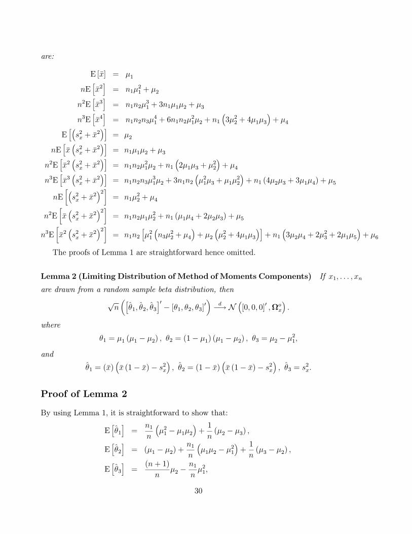
The proofs of Lemma 1 are straightforward hence omitted.

Lemma 2 (Limiting Distribution of Method of Moments Components) If x1; : : : ; xn

are drawn from a random sample beta distribution, then

pn�h�1; �2; �3

i0� [�1; �2; �3]0

�d�! N

�[0; 0; 0]0 ;ox

�:

where

�1 = �1 (�1 � �2) ; �2 = (1� �1) (�1 � �2) ; �3 = �2 � �21;

and

�1 = (�x)��x (1� �x)� s2x

�; �2 = (1� �x)

��x (1� �x)� s2x

�; �3 = s

2x:

Proof of Lemma 2

By using Lemma 1, it is straightforward to show that:

Eh�1i=

n1n

��21 � �1�2

�+1

n(�2 � �3) ;

Eh�2i= (�1 � �2) +

n1n

��1�2 � �21

�+1

n(�3 � �2) ;

Eh�3i=

(n+ 1)

n�2 �

n1n�21;

30

and

nVarh�1i= �32 � 4�41 � 4�21�22 � 4�1�22 + 4�21�2 � 4�21�3 + 8�31�2

+�21�4 + 2�1�2�3 +O�n�1

�;

nVarh�2i= �2 � 2�3 + �4 � �21 + 4�31 + �22 � 4�41 + �32 � 4�21�22�2�1�2 + 6�1�3 � 2�1�4 � 2�2�3 � 4�21�2 � 4�21�3+8�31�2 + �

21�4 + 2�1�2�3 +O

�n�1

�;

nVarh�3i= �4�41 + 12�21�2 � 4�3�1 � 5�22 + �4 +O

�n�1

�;

nCovh�1; �2

i= 4�41 � �22 � 2�31 � �32 + 4�21�22 + 2�1�2 � 3�1�3 + �1�4

+�2�3 + 2�1�22 + 4�

21�3 � 8�31�2 � �21�4 � 2�1�2�3

+O�n�1

�;

nCovh�1; �3

i= 4�41 + 2�1�3 � �1�4 � �2�3 + 6�1�22 � 8�21�2 + 2�21�3�4�31�2 +O

�n�1

�;

nCovh�2; �3

i= �4�41 + 4�31�2 + 2�31 + 6�21�2 � 2�3�21 � 6�1�22 � 5�1�2

+�4�1 + 3�22 + �3�2 + �3 � �4 +O

�n�2

�:

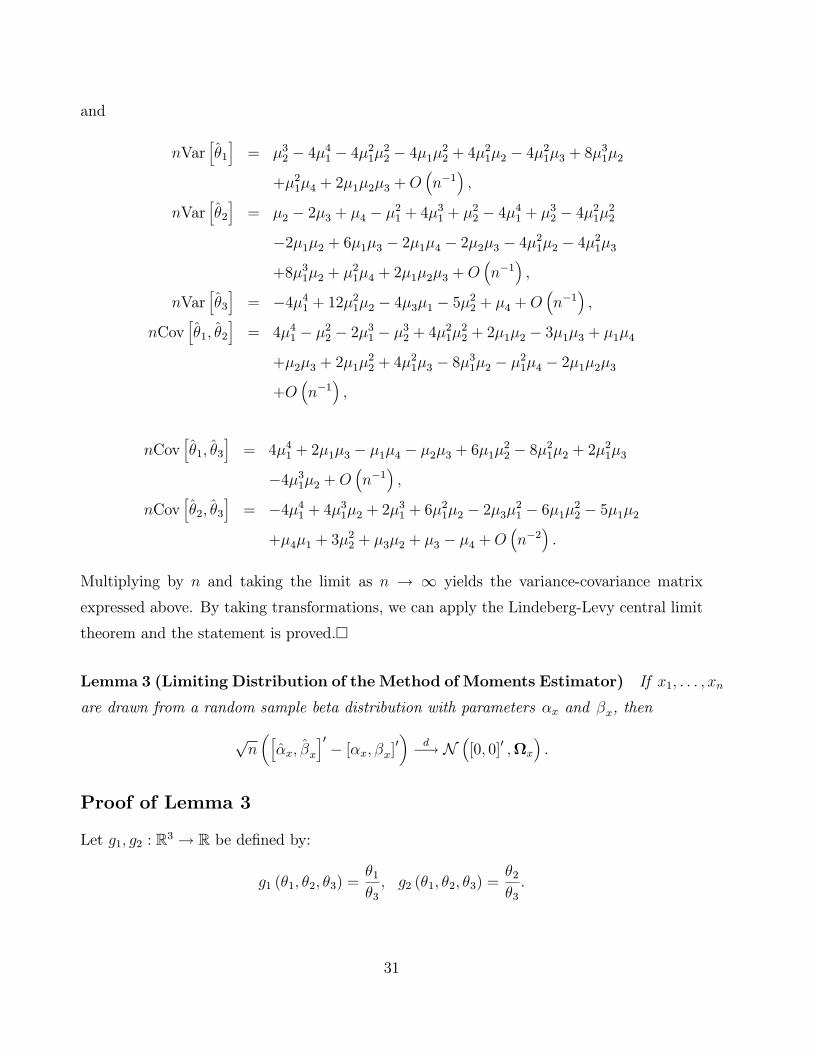
Multiplying by n and taking the limit as n ! 1 yields the variance-covariance matrix

expressed above. By taking transformations, we can apply the Lindeberg-Levy central limit

theorem and the statement is proved.�

Lemma 3 (Limiting Distribution of the Method of Moments Estimator) If x1; : : : ; xn

are drawn from a random sample beta distribution with parameters �x and �x, then

pn�h�x; �x

i0� [�x; �x]

0�

d�! N�[0; 0]0 ;x

�:

Proof of Lemma 3

Let g1; g2 : R3 ! R be de�ned by:

g1 (�1; �2; �3) =�1�3; g2 (�1; �2; �3) =

�2�3:

31

Di�erentiating, we �nd that:

@g1 (�1; �2; �3)

@x=

1

�3;@g1 (�1; �2; �3)

@y= 0;

@g1 (�1; �2; �3)

@�3= ��1

�23;

@g2 (x; y; z)

@x= 0;

@g2 (x; y; z)

@y=1

�3;@g2 (x; y; z)

@z= ��2

�23:

The Jacobian, Jox, consists of the above partial derivatives evaluated at the following values:

�1 = limn!1

Ehm21 �m1m2

i= �1 (�1 � �2) ;

�2 = limn!1

E [m1 (1�m1)� (1�m1)m2] = (1� �1) (�1 � �2) ;

�3 = limn!1

Ehm2 �m2

1

i= �2 � �21:

From here, we can use the delta method and Lemma 2 to �nd the limiting distribution ofh�x; �x

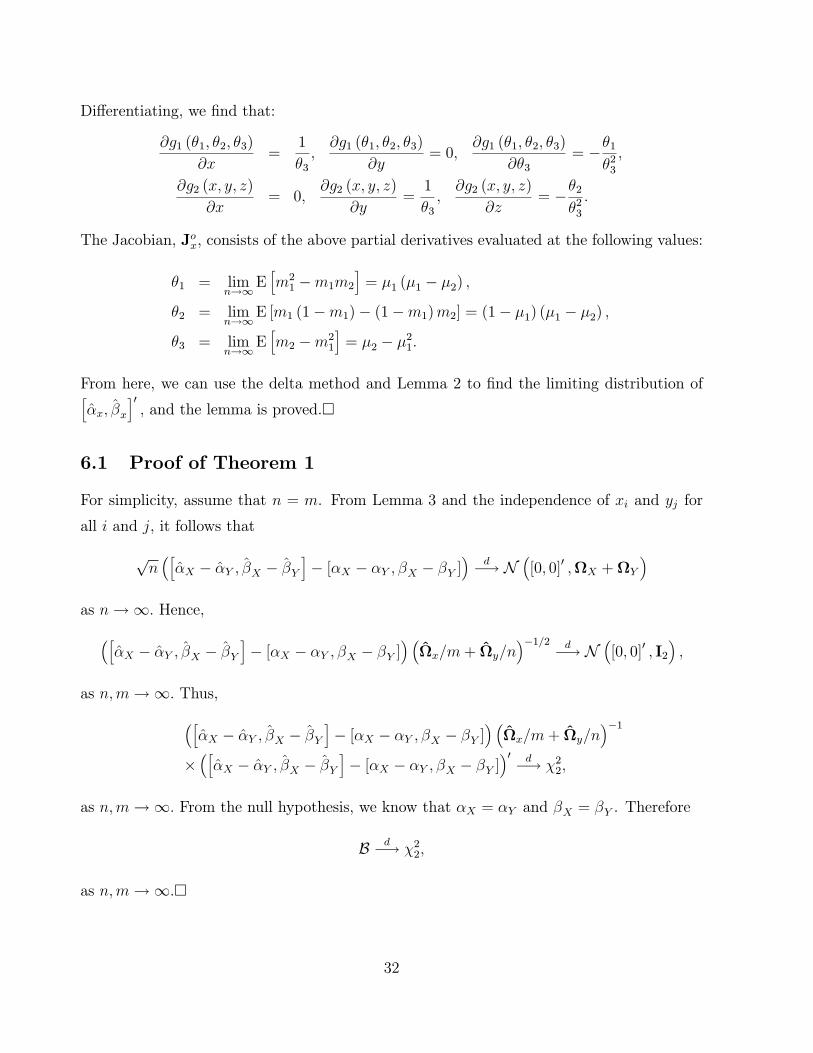
i0; and the lemma is proved.�

6.1 Proof of Theorem 1

For simplicity, assume that n = m. From Lemma 3 and the independence of xi and yj for

all i and j, it follows that

pn�h�X � �Y ; �X � �Y

i� [�X � �Y ; �X � �Y ]

�d�! N

�[0; 0]0 ;X +Y

�as n!1: Hence,�h�X � �Y ; �X � �Y

i� [�X � �Y ; �X � �Y ]

� �x=m+ y=n

��1=2 d�! N�[0; 0]0 ; I2

�;

as n;m!1: Thus,�h�X � �Y ; �X � �Y

i� [�X � �Y ; �X � �Y ]

� �x=m+ y=n

��1��h�X � �Y ; �X � �Y

i� [�X � �Y ; �X � �Y ]

�0 d�! �22;

as n;m!1: From the null hypothesis, we know that �X = �Y and �X = �Y . Therefore

B d�! �22;

as n;m!1:�

32

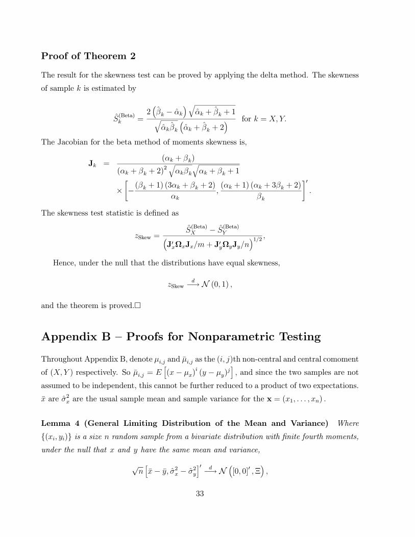
Proof of Theorem 2

The result for the skewness test can be proved by applying the delta method. The skewness

of sample k is estimated by

S(Beta)k =

2��k � �k

�q�k + �k + 1q

�k�k��k + �k + 2

� for k = X;Y:

The Jacobian for the beta method of moments skewness is,

Jk =(�k + �k)

(�k + �k + 2)2q�k�k

q�k + �k + 1

�"�(�k + 1) (3�k + �k + 2)

�k;(�k + 1) (�k + 3�k + 2)

�k

#0:

The skewness test statistic is de�ned as

zSkew =S(Beta)X � S(Beta)Y�

J0xxJx=m+ J0yyJy=n�1=2 ;

Hence, under the null that the distributions have equal skewness,

zSkewd�! N (0; 1) ;

and the theorem is proved.�

Appendix B { Proofs for Nonparametric Testing

Throughout Appendix B, denote �i;j and ��i;j as the (i; j)th non-central and central comoment

of (X;Y ) respectively. So ��i;j = Eh(x� �x)

i (y � �y)ji; and since the two samples are not

assumed to be independent, this cannot be further reduced to a product of two expectations.

�x are �2x are the usual sample mean and sample variance for the x = (x1; : : : ; xn) :

Lemma 4 (General Limiting Distribution of the Mean and Variance) Where

f(xi; yi)g is a size n random sample from a bivariate distribution with �nite fourth moments,under the null that x and y have the same mean and variance,

pnh�x� �y; �2x � �2y

i0 d�! N�[0; 0]0 ;�

�;

33

where

� =

24 ��2;0 + ��0;2 � 2��1;1 ��3;0 + ��0;3 � ��1;2 � ��2;1��3;0 + ��0;3 � ��1;2 � ��2;1 ��4;0 � ��22;0 + ��0;4 � ��20;2 � 2��2;2 + 2��0;2��2;0

35

Proof of Lemma 4

It is well-known that

E [�x] = �1;0; Eh�2xi= ��2;0;

and

nVar [�x] = ��2;0; nVarh�2xi= ��4;0 �

n� 3n� 1 ��

22;0:

It is also easy to derive:

nCov [�x; �y] = ��1;1; nCovh�x; �2x

i= ��3;0; nCov

h�x; �2y

i= ��1;2:

The only tedious term is

nCovh�2x; �

2y

i= ��2;2 � ��0;2��2;0 +

2

n� 1 ��21;1:

Using the symmetric form, we know all the components of:

� = limn!1

24 nVar [�x� �y] nCovh�x� �y; �2x � �2y

inCov

h�x� �y; �2x � �2y

inVar

h�2x � �2y

i35

=

24 ��2;0 + ��0;2 � 2��1;1 ��3;0 + ��0;3 � ��1;2 � ��2;1��3;0 + ��0;3 � ��1;2 � ��2;1 ��4;0 � ��22;0 + ��0;4 � ��20;2 � 2��2;2 + 2��0;2��2;0

35And so, by the Lindeberg-Levy central limit theorem,

pnh�x� �y; �2x � �2y

i0 d�! N2�[0; 0]0 ;�

�:

While the normality does not immediately follow as we have to apply tedious transformations

to use the Lindeberg condition, such transformations are beyond the scope of this paper,

and do not provide any useful intuition.�

34

Lemma 5 (General Limiting Distribution of the Skewness) Where f(xi; yi)gi=1;:::;nis a random sample from a bivariate distribution with �nite sixth moments, under the null

that x and y have equal skewness,

pn�Sx � Sy

�d�! N (0; !x + !y � 2!xy) ;

where

!x =1

4��52;0

�36��52;0 � 24��4;0��32;0 + 35��22;0��23;0 + 4��6;0��22;0 � 12��5;0��2;0��3;0 + 9��4;0��23;0

�;

and

!xy =1

4��5=20;2 ��

5=22;0

�12��20;2��2;0��3;1 � 18��20;2��2;1��3;0 � 18��22;0��0;3��1;2 + 12��0;2��22;0��1;3

�+

1

4��5=20;2 ��

5=22;0

��36��20;2��1;1��22;0 � 4��0;2��2;0��3;3 + 6��0;2��3;0��2;3 + 6��2;0��0;3��3;2

�+

1

4��5=20;2 ��

5=22;0

��9��0;3��3;0��2;2 + ��0;2��2;0��0;3��3;0

�:

Proof of Lemma 5

By Taylor expanding around the expectations of the moment estimators, we obtain the

approximation

Sx =��3;0

��3=22;0

+1

��3=22;0

��m3;0 � ��3;0

�� 32

��3;0

��5=22;0

��2x � ��2;0

�+Op

�n�1

�;

where �m3;0 = n (n1n2)�1Pn

i=1 (xi � �x)3 : Notice that E �m3;0 = ��3;0: So it is obvious that

E[�3x] = �3x +O (n�1) : So, the only thorny issue is deriving the variance-covariance matrix

of [�3x; �3y]0,

VarhSxi=

1

��32;0Var [ �m3;0] +

9

4

��23;0��52;0

Varh�2xi� 3

��3;0��42;0

Covh�m3;0; �

2x

i+O

�n�2

�:

Although the calculation is rather tedious, it is straightforward to obtain the following,

Var [ �m3;0] = n�1���6;0 � ��23;0 � 6��2;0��4;0 + 9��32;0

�+O

�n�2

�;

Covh�m3;0; �

2x

i= n�1

���5;0 � 4��2;0��3;0

�+O

�n�2

�:

35

Hence,

VarhSxi=

1

4n��52;0

�36��52;0 � 24��4;0��32;0 + 35��22;0��23;0 + 4��6;0��22;0 � 12��5;0��2;0��3;0 + 9��4;0��23;0

�+

1

4n��52;0

��12��5;0��2;0��3;0 + 9��4;0��23;0

�+O

�n�2

�:

To �nd the covariance, we compute:

Cov [ �m3;0; �m0;3] = n�1���3;3 � ��0;3��3;0 � 3��0;2��3;1 � 3��1;3��2;0 + 9��0;2��1;1��2;0

�+O

�n�2

�;

Covh�m3;0; �

2y

i= n�1

���3;2 � ��0;2��3;0 � 3��1;2��2;0

�+O

�n�2

�:

So,

CovhSx; Sy

i=

1

4n��5=20;2 ��

5=22;0

�12��20;2��2;0��3;1 � 18��20;2��2;1��3;0 � 18��22;0��0;3��1;2 + 12��0;2��22;0��1;3

�+

+1

4n��5=20;2 ��

5=22;0

��36��20;2��1;1��22;0 � 4��0;2��2;0��3;3 + 6��0;2��3;0��2;3 + 6��2;0��0;3��3;2

�+

1

4n��5=20;2 ��

5=22;0

��9��0;3��3;0��2;2 + ��0;2��2;0��0;3��3;0

�+O

�n�2

�:

Thus, under the null that X and Y have equal skewness,

pn�Sx � Sy

�d�! N (0; !x + !y � 2!xy) ;

and the lemma is proved.�

36