BlinkDB: Queries with Bounded Errors andBounded Response Times on Very Large Data

Sameer Agarwal†, Barzan Mozafari◦, Aurojit Panda†, Henry Milner†, Samuel Madden◦, Ion Stoica∗†

†University of California, Berkeley ◦Massachusetts Institute of Technology ∗Conviva Inc.{sameerag, apanda, henrym, istoica}@cs.berkeley.edu, {barzan, madden}@csail.mit.edu

AbstractIn this paper, we present BlinkDB, a massively parallel, ap-proximate query engine for running interactive SQL querieson large volumes of data. BlinkDB allows users to trade-off query accuracy for response time, enabling interactivequeries over massive data by running queries on data sam-ples and presenting results annotated with meaningful errorbars. To achieve this, BlinkDB uses two key ideas: (1) anadaptive optimization framework that builds and maintainsa set of multi-dimensional stratified samples from originaldata over time, and (2) a dynamic sample selection strat-egy that selects an appropriately sized sample based on aquery’s accuracy or response time requirements. We evalu-ate BlinkDB against the well-known TPC-H benchmarks anda real-world analytic workload derived from Conviva Inc., acompany that manages video distribution over the Internet.Our experiments on a 100 node cluster show that BlinkDB

can answer queries on up to 17 TBs of data in less than 2seconds (over 200× faster than Hive), within an error of 2-10%.

1. IntroductionModern data analytics applications involve computing ag-gregates over a large number of records to roll-up web clicks,online transactions, content downloads, and other featuresalong a variety of different dimensions, including demo-graphics, content type, region, and so on. Traditionally, suchqueries have been executed using sequential scans over alarge fraction of a database. Increasingly, new applicationsdemand near real-time response rates. Examples may in-clude applications that (i) update ads on a website based ontrends in social networks like Facebook and Twitter, or (ii)determine the subset of users experiencing poor performancebased on their service provider and/or geographic location.Over the past two decades a large number of approxima-tion techniques have been proposed, which allow for fast

Permission to make digital or hard copies of all or part of this work for personal orclassroom use is granted without fee provided that copies are not made or distributedfor profit or commercial advantage and that copies bear this notice and the full citationon the first page. To copy otherwise, to republish, to post on servers or to redistributeto lists, requires prior specific permission and/or a fee.Eurosys’13 April 15-17, 2013, Prague, Czech RepublicCopyright © 2013 ACM 978-1-4503-1994-2/13/04. . . $15.00

processing of large amounts of data by trading result ac-curacy for response time and space. These techniques in-clude sampling [10, 14], sketches [12], and on-line aggre-gation [15]. To illustrate the utility of such techniques, con-sider the following simple query that computes the averageSessionTime over all users originating in New York:

SELECT AVG(SessionTime)

FROM Sessions

WHERE City = ‘New York’

Suppose the Sessions table contains 100 million tuplesfor New York, and cannot fit in memory. In that case, theabove query may take a long time to execute, since diskreads are expensive, and such a query would need multipledisk accesses to stream through all the tuples. Suppose weinstead executed the same query on a sample containing only10, 000 New York tuples, such that the entire sample fits inmemory. This would be orders of magnitude faster, whilestill providing an approximate result within a few percent ofthe actual value, an accuracy good enough for many practicalpurposes. Using sampling theory we could even provideconfidence bounds on the accuracy of the answer [16].

Previously described approximation techniques make dif-ferent trade-offs between efficiency and the generality ofthe queries they support. At one end of the spectrum, ex-isting sampling and sketch based solutions exhibit low spaceand time complexity, but typically make strong assumptionsabout the query workload (e.g., they assume they know theset of tuples accessed by future queries and aggregationfunctions used in queries). As an example, if we know allfuture queries are on large cities, we could simply maintainrandom samples that omit data about smaller cities.

At the other end of the spectrum, systems like online ag-gregation (OLA) [15] make fewer assumptions about thequery workload, at the expense of highly variable perfor-mance. Using OLA, the above query will likely finish muchfaster for sessions in New York (i.e., the user might besatisfied with the result accuracy, once the query sees thefirst 10, 000 sessions from New York) than for sessions inGalena, IL, a town with fewer than 4, 000 people. In fact,for such a small town, OLA may need to read the entire tableto compute a result with satisfactory error bounds.

In this paper, we argue that none of the previous solutionsare a good fit for today’s big data analytics workloads. OLA

provides relatively poor performance for queries on rare tu-ples, while sampling and sketches make strong assumptionsabout the predictability of workloads or substantially limitthe types of queries they can execute.

To this end, we propose BlinkDB, a distributed sampling-based approximate query processing system that strives toachieve a better balance between efficiency and generalityfor analytics workloads. BlinkDB allows users to pose SQL-based aggregation queries over stored data, along with re-sponse time or error bound constraints. As a result, queriesover multiple terabytes of data can be answered in seconds,accompanied by meaningful error bounds relative to the an-swer that would be obtained if the query ran on the fulldata. In contrast to most existing approximate query solu-tions (e.g., [10]), BlinkDB supports more general queriesas it makes no assumptions about the attribute values inthe WHERE, GROUP BY, and HAVING clauses, or the distribu-tion of the values used by aggregation functions. Instead,BlinkDB only assumes that the sets of columns used byqueries in WHERE, GROUP BY, and HAVING clauses are sta-ble over time. We call these sets of columns “query columnsets” or QCSs in this paper.

BlinkDB consists of two main modules: (i) Sample Cre-ation and (ii) Sample Selection. The sample creation mod-ule creates stratified samples on the most frequently usedQCSs to ensure efficient execution for queries on rare values.By stratified, we mean that rare subgroups (e.g., Galena,IL) are over-represented relative to a uniformly random sam-ple. This ensures that we can answer queries about any sub-group, regardless of its representation in the underlying data.

We formulate the problem of sample creation as an opti-mization problem. Given a collection of past QCS and theirhistorical frequencies, we choose a collection of stratifiedsamples with total storage costs below some user config-urable storage threshold. These samples are designed to ef-ficiently answer queries with the same QCSs as past queries,and to provide good coverage for future queries over sim-ilar QCS. If the distribution of QCSs is stable over time,our approach creates samples that are neither over- norunder-specialized for the query workload. We show thatin real-world workloads from Facebook Inc. and ConvivaInc., QCSs do re-occur frequently and that stratified samplesbuilt using historical patterns of QCS usage continue to per-form well for future queries. This is in contrast to previousoptimization-based sampling systems that assume completeknowledge of the tuples accessed by queries at optimizationtime.

Based on a query’s error/response time constraints, thesample selection module dynamically picks a sample onwhich to run the query. It does so by running the queryon multiple smaller sub-samples (which could potentially bestratified across a range of dimensions) to quickly estimatequery selectivity and choosing the best sample to satisfyspecified response time and error bounds. It uses an Error-

Latency Profile heuristic to efficiently choose the sample thatwill best satisfy the user-specified error or time bounds.

We implemented BlinkDB1 on top of Hive/Hadoop [22](as well as Shark [13], an optimized Hive/Hadoop frame-work that caches input/ intermediate data). Our implementa-tion requires minimal changes to the underlying query pro-cessing system. We validate its effectiveness on a 100 nodecluster, using both the TPC-H benchmarks and a real-worldworkload derived from Conviva. Our experiments show thatBlinkDB can answer a range of queries within 2 seconds on17 TB of data within 90-98% accuracy, which is two or-ders of magnitude faster than running the same queries onHive/Hadoop. In summary, we make the following contri-butions:

• We use a column-set based optimization framework tocompute a set of stratified samples (in contrast to ap-proaches like AQUA [6] and STRAT [10], which com-pute only a single sample per table). Our optimizationtakes into account: (i) the frequency of rare subgroups inthe data, (ii) the column sets in the past queries, and (iii)the storage overhead of each sample. (§4)

• We create error-latency profiles (ELPs) for each queryat runtime to estimate its error or response time on eachavailable sample. This heuristic is then used to select themost appropriate sample to meet the query’s responsetime or accuracy requirements. (§5)

• We show how to integrate our approach into an existingparallel query processing framework (Hive) with mini-mal changes. We demonstrate that by combining theseideas together, BlinkDB provides bounded error and la-tency for a wide range of real-world SQL queries, and itis robust to variations in the query workload. (§6)

2. BackgroundAny sampling based query processor, including BlinkDB,must decide what types of samples to create. The samplecreation process must make some assumptions about the na-ture of the future query workload. One common assumptionis that future queries will be similar to historical queries.While this assumption is broadly justified, it is necessary tobe precise about the meaning of “similarity” when buildinga workload model. A model that assumes the wrong kind ofsimilarity will lead to a system that “over-fits” to past queriesand produces samples that are ineffective at handling futureworkloads. This choice of model of past workloads is oneof the key differences between BlinkDB and prior work. Inthe rest of this section, we present a taxonomy of workloadmodels, discuss our approach, and show that it is reasonableusing experimental evidence from a production system.

1 http://blinkdb.org

2.1 Workload TaxonomyOffline sample creation, caching, and virtually any othertype of database optimization assumes a target workload thatcan be used to predict future queries. Such a model can eitherbe trained on past data, or based on information provided byusers. This can range from an ad-hoc model, which makes noassumptions about future queries, to a model which assumesthat all future queries are known a priori. As shown in Fig. 1,we classify possible approaches into one of four categories:

Flexibility

Efficiency Low flexibility / High Efficiency

High flexibility / Low Efficiency

Predictable    Queries  

Predictable    Query  Predicates  

Predictable    Query  Column  Sets  

Unpredictable    Queries  

Figure 1. Taxonomy of workload models.

1. Predictable Queries: At the most restrictive end ofthe spectrum, one can assume that all future queries areknown in advance, and use data structures specially designedfor these queries. Traditional databases use such a modelfor lossless synopsis [12] which can provide extremely fastresponses for certain queries, but cannot be used for anyother queries. Prior work in approximate databases has alsoproposed using lossy sketches (including wavelets and his-tograms) [14].

2. Predictable Query Predicates: A slightly more flex-ible model is one that assumes that the frequencies of groupand filter predicates — both the columns and the values inWHERE, GROUP BY, and HAVING clauses — do not changeover time. For example, if 5% of past queries include onlythe filter WHERE City = ‘New York’ and no other groupor filter predicates, then this model predicts that 5% of futurequeries will also include only this filter. Under this model,it is possible to predict future filter predicates by observinga prior workload. This model is employed by materializedviews in traditional databases. Approximate databases, suchas STRAT [10] and SciBORQ [21], have similarly relied onprior queries to determine the tuples that are likely to be usedin future queries, and to create samples containing them.

3. Predictable QCSs: Even greater flexibility is pro-vided by assuming a model where the frequency of the setsof columns used for grouping and filtering does not changeover time, but the exact values that are of interest in thosecolumns are unpredictable. We term the columns used forgrouping and filtering in a query the query column set, orQCS, for the query. For example, if 5% of prior queriesgrouped or filtered on the QCS {City}, this model assumesthat 5% of future queries will also group or filter on this QCS,though the particular predicate may vary. This model can beused to decide the columns on which building indices wouldoptimize data access. Prior work [20] has shown that a sim-ilar model can be used to improve caching performance inOLAP systems. AQUA [4], an approximate query database

based on sampling, uses the QCS model. (See §8 for a com-parison between AQUA and BlinkDB).

4. Unpredictable Queries: Finally, the most generalmodel assumes that queries are unpredictable. Given this as-sumption, traditional databases can do little more than justrely on query optimizers which operate at the level of a sin-gle query. In approximate databases, this workload modeldoes not lend itself to any “intelligent” sampling, leaving onewith no choice but to uniformly sample data. This model isused by On-Line Aggregation (OLA) [15], which relies onstreaming data in random order.

While the unpredictable query model is the most flex-ible one, it provides little opportunity for an approximatequery processing system to efficiently sample the data. Fur-thermore, prior work [11, 19] has argued that OLA per-formance’s on large clusters (the environment on whichBlinkDB is intended to run) falls short. In particular, access-ing individual rows randomly imposes significant schedul-ing and communication overheads, while accessing data atthe HDFS block2 level may skew the results.

As a result, we use the model of predictable QCSs. Aswe will show, this model provides enough information toenable efficient pre-computation of samples, and it leads tosamples that generalize well to future workloads in our ex-periments. Intuitively, such a model also seems to fit in withthe types of exploratory queries that are commonly executedon large scale analytical clusters. As an example, considerthe operator of a video site who wishes to understand whattypes of videos are popular in a given region. Such a studymay require looking at data from thousands of videos andhundreds of geographic regions. While this study could re-sult in a very large number of distinct queries, most will useonly two columns, video title and viewer location, for group-ing and filtering. Next, we present empirical evidence basedon real world query traces from Facebook Inc. and ConvivaInc. to support our claims.

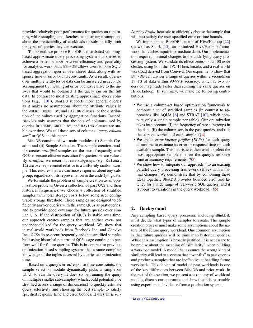
2.2 Query Patterns in a Production ClusterTo empirically test the validity of the predictable QCS modelwe analyze a trace of 18, 096 queries from 30 days of queriesfrom Conviva and a trace of 69, 438 queries constitutinga random, but representative, fraction of 7 days’ workloadfrom Facebook to determine the frequency of QCSs.

Fig. 2(a) shows the distribution of QCSs across all queriesfor both workloads. Surprisingly, over 90% of queries arecovered by 10% and 20% of unique QCSs in the tracesfrom Conviva and Facebook respectively. Only 182 uniqueQCSs cover all queries in the Conviva trace and 455 uniqueQCSs span all the queries in the Facebook trace. Further-more, if we remove the QCSs that appear in less than 10queries, we end up with only 108 and 211 QCSs covering17, 437 queries and 68, 785 queries from Conviva and Face-book workloads, respectively. This suggests that, for real-

2 Typically, these blocks are 64− 1024 MB in size.

0.1

0.2

0.3

0.4

0.5

0.6

0.7

0.8

0.9

1

0 20 40 60 80 100

Fract

ion o

f Q

ueri

es

(CD

F)

Unique Query Templates (%)

Conviva Queries (2 Years)Facebook Queries (1 week)

(a) QCS Distribution

0

10

20

30

40

50

60

70

80

90

100

0 20 40 60 80 100

New

Uniq

ue

Tem

pla

tes

Seen (

%)

Incoming Queries (%)

Conviva Queries (2 Years)Facebook Queries (1 week)

(b) QCS Stability

0.1

0.2

0.3

0.4

0.5

0.6

0.7

0.8

0.9

1

0.001 0.01 0.1 1 10 100 1000 10000 100000 1e+06

Fract

ion o

f Jo

in Q

ueri

es

(CD

F)

Size of Dimension Table(s) (GB)

Facebook Queries (1 Week)

(c) Dimension table size CDFFigure 2. 2(a) and 2(b) show the distribution and stability of QCSs respectively across all queries in the Conviva andFacebook traces. 2(c) shows the distribution of join queries with respect to the size of dimension tables.

world production workloads, QCSs represent an excellentmodel of future queries.

Fig. 2(b) shows the number of unique QCSs versus thequeries arriving in the system. We define unique QCSs asQCSs that appear in more than 10 queries. For the Con-viva trace, after only 6% of queries we already see close to60% of all QCSs, and after 30% of queries have arrived, wesee almost all QCSs — 100 out of 108. Similarly, for theFacebook trace, after 12% of queries, we see close to 60%of all QCSs, and after only 40% queries, we see almost allQCSs — 190 out of 211. This shows that QCSs are relativelystable over time, which suggests that the past history is agood predictor for the future workload.

3. System Overview

Sample'Selection'

TABLE'

Distributed'Cache'

Distributed'Filesystem'

Original''Data'

Shark'

'SELECT COUNT(*)! FROM TABLE!WHERE (city=“NY”)!LIMIT 1s;!

HiveQL/SQL'Query'

Result:(1,101,822(±(2,105&&(95%(confidence)(

Sample'Crea

tion'&'

Mainten

ance

'

Figure 3. BlinkDB architecture.

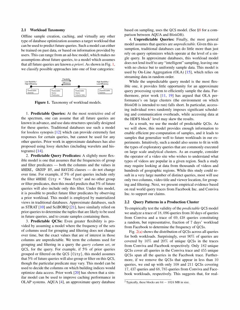
Fig. 3 shows the overall architecture of BlinkDB. BlinkDBextends the Apache Hive framework [22] by adding two ma-jor components to it: (1) an offline sampling module thatcreates and maintains samples over time, and (2) a run-timesample selection module that creates an Error-Latency Pro-file (ELP) for queries. To decide on the samples to create, weuse the QCSs that appear in queries (we present a more pre-cise formulation of this mechanism in §4.) Once this choiceis made, we rely on distributed reservoir sampling3 [23] orbinomial sampling techniques to create a range of uniformand stratified samples across a number of dimensions.

At run-time, we employ ELP to decide the sample to runthe query. The ELP characterizes the rate at which the error

3 Reservoir sampling is a family of randomized algorithms for creatingfixed-sized random samples from streaming data.

(or response time) decreases (or increases) as the size of thesample on which the query operates increases. This is usedto select a sample that best satisfies the user’s constraints.We describe ELP in detail in §5. BlinkDB also augmentsthe query parser, optimizer, and a number of aggregationoperators to allow queries to specify bounds on error, orexecution time.

3.1 Supported QueriesBlinkDB supports a slightly constrained set of SQL-style

declarative queries, imposing constraints that are similar toprior work [10]. In particular, BlinkDB can currently provideapproximate results for standard SQL aggregate queries in-volving COUNT, AVG, SUM and QUANTILE. Queries involv-ing these operations can be annotated with either an errorbound, or a time constraint. Based on these constraints, thesystem selects an appropriate sample, of an appropriate size,as explained in §5.

As an example, let us consider querying a tableSessions, with five columns, SessionID, Genre, OS,City, and URL, to determine the number of sessions in whichusers viewed content in the “western” genre, grouped byOS. The query:

SELECT COUNT(*)

FROM Sessions

WHERE Genre = ‘western’

GROUP BY OS

ERROR WITHIN 10% AT CONFIDENCE 95%

will return the count for each GROUP BY key, with each counthaving relative error of at most ±10% at a 95% confidencelevel. Alternatively, a query of the form:

SELECT COUNT(*)

FROM Sessions

WHERE Genre = ‘western’

GROUP BY OS

WITHIN 5 SECONDS

will return the most accurate results for each GROUP BY keyin 5 seconds, along with a 95% confidence interval for therelative error of each result.

While BlinkDB does not currently support arbitrary joinsand nested SQL queries, we find that this is usually not a hin-

drance. This is because any query involving nested queriesor joins can be flattened to run on the underlying data. How-ever, we do provide support for joins in some settings whichare commonly used in distributed data warehouses. In par-ticular, BlinkDB can support joining a large, sampled facttable, with smaller tables that are small enough to fit in themain memory of any single node in the cluster. This is oneof the most commonly used form of joins in distributed datawarehouses. For instance, Fig. 2(c) shows the distribution ofthe size of dimension tables (i.e., all tables except the largest)across all queries in a week’s trace from Facebook. We ob-serve that 70% of the queries involve dimension tables thatare less than 100 GB in size. These dimension tables can beeasily cached in the cluster memory, assuming a cluster con-sisting of hundreds or thousands of nodes, where each nodehas at least 32 GB RAM. It would also be straightforward toextend BlinkDB to deal with foreign key joins between twosampled tables (or a self join on one sampled table) whereboth tables have a stratified sample on the set of columnsused for joins. We are also working on extending our querymodel to support more general queries, specifically focusingon more complicated user defined functions, and on nestedqueries.

4. Sample CreationBlinkDB creates a set of samples to accurately and quicklyanswer queries. In this section, we describe the sample cre-ation process in detail. First, in §4.1, we discuss the creationof a stratified sample on a given set of columns. We showhow a query’s accuracy and response time depends on theavailability of stratified samples for that query, and evaluatethe storage requirements of our stratified sampling strategyfor various data distributions. Stratified samples are useful,but carry storage costs, so we can only build a limited num-ber of them. In §4.2 we formulate and solve an optimizationproblem to decide on the sets of columns on which we buildsamples.

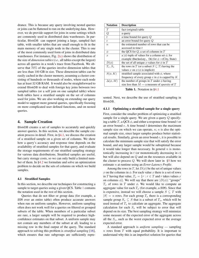
4.1 Stratified SamplesIn this section, we describe our techniques for constructing asample to target queries using a given QCS. Table 1 containsthe notation used in the rest of this section.

Queries that do not filter or group data (for example, aSUM over an entire table) often produce accurate answerswhen run on uniform samples. However, uniform samplingoften does not work well for a queries on filtered or groupedsubsets of the table. When members of a particular subsetare rare, a larger sample will be required to produce high-confidence estimates on that subset. A uniform sample maynot contain any members of the subset at all, leading to amissing row in the final output of the query. The standardapproach to solving this problem is stratified sampling [16],which ensures that rare subgroups are sufficiently repre-

Notation DescriptionT fact (original) tableQ a queryt a time bound for query Qe an error bound for query Qn the estimated number of rows that can be

accessed in time tφ the QCS for Q, a set of columns in Tx a |φ|-tuple of values for a column set φ, for

example (Berkeley, CA) for φ =(City, State)D(φ) the set of all unique x-values for φ in TTx, Sx the rows in T (or a subset S ⊆ T ) having the

values x on φ (φ is implicit)S(φ,K) stratified sample associated with φ, where

frequency of every group x in φ is capped by K∆(φ,M) the number of groups in T under φ having

size less than M — a measure of sparsity of T

Table 1. Notation in §4.1

sented. Next, we describe the use of stratified sampling inBlinkDB.

4.1.1 Optimizing a stratified sample for a single queryFirst, consider the smaller problem of optimizing a stratifiedsample for a single query. We are given a query Q specify-ing a table T , a QCS φ, and either a response time bound t oran error bound e. A time bound t determines the maximumsample size on which we can operate, n; n is also the opti-mal sample size, since larger samples produce better statisti-cal results. Similarly, given an error bound e, it is possible tocalculate the minimum sample size that will satisfy the errorbound, and any larger sample would be suboptimal becauseit would take longer than necessary. In general n is mono-tonically increasing in t (or monotonically decreasing in e)but will also depend on Q and on the resources available inthe cluster to process Q. We will show later in §5 how weestimate n at runtime using an Error-Latency Profile.

Among the rows in T , letD(φ) be the set of unique valuesx on the columns in φ. For each value x there is a set of rowsin T having that value, Tx = {r : r ∈ T and r takes values xon columns φ}. We will say that there are |D(φ)| “groups”Tx of rows in T under φ. We would like to compute anaggregate value for each Tx (for example, a SUM). Since thatis expensive, instead we will choose a sample S ⊆ T with|S| = n rows. For each group Tx there is a correspondingsample group Sx ⊆ S that is a subset of Tx, which will beused instead of Tx to calculate an aggregate. The aggregatecalculation for each Sx will be subject to error that willdepend on its size. The best sampling strategy will minimizesome measure of the expected error of the aggregate acrossall the Sx, such as the worst expected error or the averageexpected error.

A standard approach is uniform sampling — samplingn rows from T with equal probability. It is important tounderstand why this is an imperfect solution for queries that

compute aggregates on groups. A uniform random sampleallocates a random number of rows to each group. The sizeof sample group Sx has a hypergeometric distribution withn draws, population size |T |, and |Tx| possibilities for thegroup to be drawn. The expected size of Sx is n |Tx||T | , whichis proportional to |Tx|. For small |Tx|, there is a chance that|Sx| is very small or even zero, so the uniform samplingscheme can miss some groups just by chance. There are 2things going wrong:

1. The sample size assigned to a group depends on its sizein T . If we care about the error of each aggregate equally,it is not clear why we should assign more samples to Sxjust because |Tx| is larger.

2. Choosing sample sizes at random introduces the possibil-ity of missing or severely under-representing groups. Theprobability of missing a large group is vanishingly small,but the probability of missing a small group is substantial.

This problem has been studied before. Briefly, since errordecreases at a decreasing rate as sample size increases, thebest choice simply assigns equal sample size to each groups.In addition, the assignment of sample sizes is deterministic,not random. A detailed proof is given by Acharya et al. [4].This leads to the following algorithm for sample selection:

1. Compute group counts: To each x ∈x0, ..., x|D(φ)|−1, assign a count, forming a |D(φ)|-vector of counts N∗n. Compute N∗n as follows: LetN(n′) = (min(b n′

|D(φ)|c, |Tx0|),min(b n′

|D(φ)|c, |Tx1|, ...),

the optimal count-vector for a total sample size n′. Thenchoose N∗n = N(max{n′ : ||N(n′)||1 ≤ n}). In words,our samples cap the count of each group at some valueb n′

|D(φ)|c. In the future we will use the name K for the cap

size b n′

|D(φ)|c.2. Take samples: For each x, sample N∗nx rows uni-

formly at random without replacement from Tx, forming thesample Sx. Note that when |Tx| = N∗nx, our sample includesall the rows of Tx, and there will be no sampling error forthat group.

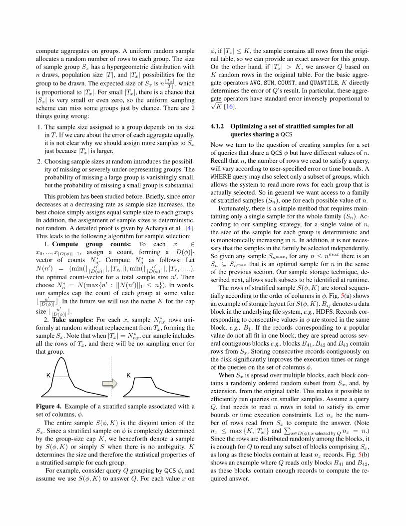
V(φ) S(φ)

K K

φ

Figure 4. Example of a stratified sample associated with aset of columns, φ.

The entire sample S(φ,K) is the disjoint union of theSx. Since a stratified sample on φ is completely determinedby the group-size cap K, we henceforth denote a sampleby S(φ,K) or simply S when there is no ambiguity. Kdetermines the size and therefore the statistical properties ofa stratified sample for each group.

For example, consider query Q grouping by QCS φ, andassume we use S(φ,K) to answer Q. For each value x on

φ, if |Tx| ≤ K, the sample contains all rows from the origi-nal table, so we can provide an exact answer for this group.On the other hand, if |Tx| > K, we answer Q based onK random rows in the original table. For the basic aggre-gate operators AVG, SUM, COUNT, and QUANTILE, K directlydetermines the error of Q’s result. In particular, these aggre-gate operators have standard error inversely proportional to√K [16].

4.1.2 Optimizing a set of stratified samples for allqueries sharing a QCS

Now we turn to the question of creating samples for a setof queries that share a QCS φ but have different values of n.Recall that n, the number of rows we read to satisfy a query,will vary according to user-specified error or time bounds. AWHERE query may also select only a subset of groups, whichallows the system to read more rows for each group that isactually selected. So in general we want access to a familyof stratified samples (Sn), one for each possible value of n.

Fortunately, there is a simple method that requires main-taining only a single sample for the whole family (Sn). Ac-cording to our sampling strategy, for a single value of n,the size of the sample for each group is deterministic andis monotonically increasing in n. In addition, it is not neces-sary that the samples in the family be selected independently.So given any sample Snmax , for any n ≤ nmax there is anSn ⊆ Snmax that is an optimal sample for n in the senseof the previous section. Our sample storage technique, de-scribed next, allows such subsets to be identified at runtime.

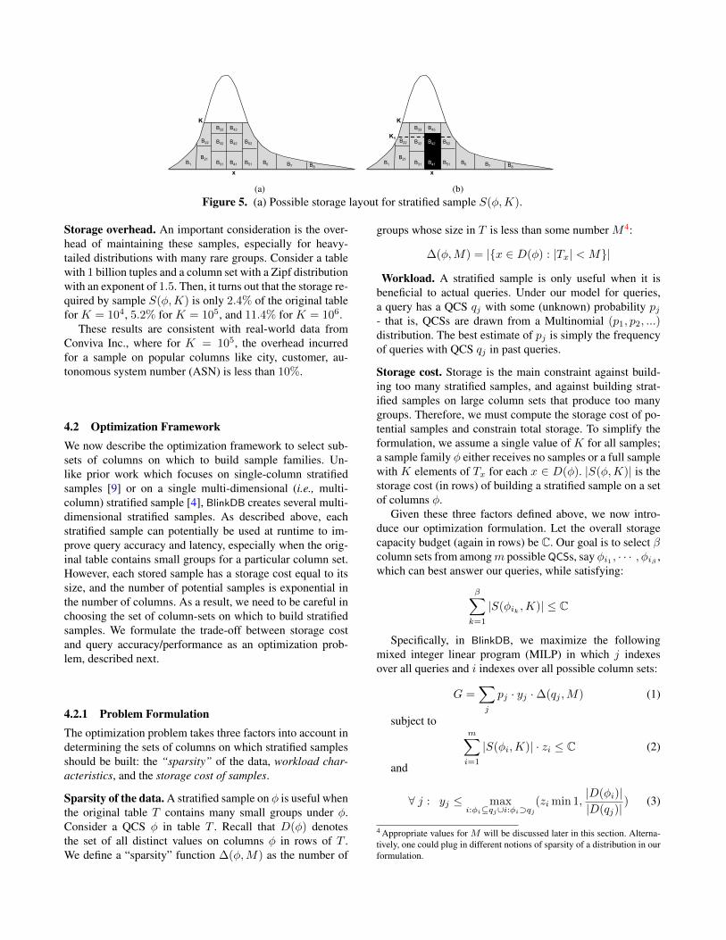
The rows of stratified sample S(φ,K) are stored sequen-tially according to the order of columns in φ. Fig. 5(a) showsan example of storage layout for S(φ,K).Bij denotes a datablock in the underlying file system, e.g., HDFS. Records cor-responding to consecutive values in φ are stored in the sameblock, e.g., B1. If the records corresponding to a popularvalue do not all fit in one block, they are spread across sev-eral contiguous blocks e.g., blocksB41,B42 andB43 containrows from Sx. Storing consecutive records contiguously onthe disk significantly improves the execution times or rangeof the queries on the set of columns φ.

When Sx is spread over multiple blocks, each block con-tains a randomly ordered random subset from Sx, and, byextension, from the original table. This makes it possible toefficiently run queries on smaller samples. Assume a queryQ, that needs to read n rows in total to satisfy its errorbounds or time execution constraints. Let nx be the num-ber of rows read from Sx to compute the answer. (Notenx ≤ max {K, |Tx|} and

∑x∈D(φ),x selected byQ nx = n.)

Since the rows are distributed randomly among the blocks, itis enough for Q to read any subset of blocks comprising Sx,as long as these blocks contain at least nx records. Fig. 5(b)shows an example where Q reads only blocks B41 and B42,as these blocks contain enough records to compute the re-quired answer.

K

B1

B21

B22

B31

B32

B33

B41

B42

B51

B52

B6 B7 B8

B43

x

(a)

K

B1

B21

B22

B31

B32

B33

B51

B52

B6 B7 B8

B43

K1 B42

B41

x

(b)Figure 5. (a) Possible storage layout for stratified sample S(φ,K).

Storage overhead. An important consideration is the over-head of maintaining these samples, especially for heavy-tailed distributions with many rare groups. Consider a tablewith 1 billion tuples and a column set with a Zipf distributionwith an exponent of 1.5. Then, it turns out that the storage re-quired by sample S(φ,K) is only 2.4% of the original tablefor K = 104, 5.2% for K = 105, and 11.4% for K = 106.

These results are consistent with real-world data fromConviva Inc., where for K = 105, the overhead incurredfor a sample on popular columns like city, customer, au-tonomous system number (ASN) is less than 10%.

4.2 Optimization FrameworkWe now describe the optimization framework to select sub-sets of columns on which to build sample families. Un-like prior work which focuses on single-column stratifiedsamples [9] or on a single multi-dimensional (i.e., multi-column) stratified sample [4], BlinkDB creates several multi-dimensional stratified samples. As described above, eachstratified sample can potentially be used at runtime to im-prove query accuracy and latency, especially when the orig-inal table contains small groups for a particular column set.However, each stored sample has a storage cost equal to itssize, and the number of potential samples is exponential inthe number of columns. As a result, we need to be careful inchoosing the set of column-sets on which to build stratifiedsamples. We formulate the trade-off between storage costand query accuracy/performance as an optimization prob-lem, described next.

4.2.1 Problem FormulationThe optimization problem takes three factors into account indetermining the sets of columns on which stratified samplesshould be built: the “sparsity” of the data, workload char-acteristics, and the storage cost of samples.

Sparsity of the data. A stratified sample on φ is useful whenthe original table T contains many small groups under φ.Consider a QCS φ in table T . Recall that D(φ) denotesthe set of all distinct values on columns φ in rows of T .We define a “sparsity” function ∆(φ,M) as the number of

groups whose size in T is less than some number M 4:

∆(φ,M) = |{x ∈ D(φ) : |Tx| < M}|

Workload. A stratified sample is only useful when it isbeneficial to actual queries. Under our model for queries,a query has a QCS qj with some (unknown) probability pj- that is, QCSs are drawn from a Multinomial (p1, p2, ...)distribution. The best estimate of pj is simply the frequencyof queries with QCS qj in past queries.

Storage cost. Storage is the main constraint against build-ing too many stratified samples, and against building strat-ified samples on large column sets that produce too manygroups. Therefore, we must compute the storage cost of po-tential samples and constrain total storage. To simplify theformulation, we assume a single value of K for all samples;a sample family φ either receives no samples or a full samplewith K elements of Tx for each x ∈ D(φ). |S(φ,K)| is thestorage cost (in rows) of building a stratified sample on a setof columns φ.

Given these three factors defined above, we now intro-duce our optimization formulation. Let the overall storagecapacity budget (again in rows) be C. Our goal is to select βcolumn sets from amongm possible QCSs, say φi1 , · · · , φiβ ,which can best answer our queries, while satisfying:

β∑k=1

|S(φik ,K)| ≤ C

Specifically, in BlinkDB, we maximize the followingmixed integer linear program (MILP) in which j indexesover all queries and i indexes over all possible column sets:

G =∑j

pj · yj ·∆(qj ,M) (1)

subject tom∑i=1

|S(φi,K)| · zi ≤ C (2)

and

∀ j : yj ≤ maxi:φi⊆qj∪i:φi⊃qj

(zi min 1,|D(φi)||D(qj)|

) (3)

4 Appropriate values for M will be discussed later in this section. Alterna-tively, one could plug in different notions of sparsity of a distribution in ourformulation.

where 0 ≤ yj ≤ 1 and zi ∈ {0, 1} are variables.Here, zi is a binary variable determining whether a sam-

ple family should be built or not, i.e., when zi = 1, we builda sample family on φi; otherwise, when zi = 0, we do not.

The goal function (1) aims to maximize the weighted sumof the coverage of the QCSs of the queries, qj . If we createa stratified sample S(φi,K), the coverage of this samplefor qj is defined as the probability that a given value x ofcolumns qj is also present among the rows of S(φi,K). Ifφi ⊇ qj , then qj is covered exactly, but φi ⊂ qj can also beuseful by partially covering qj . At runtime, if no stratifiedsample is available that exactly covers a the QCS for a query,a partially-covering QCS may be used instead. In particular,the uniform sample is a degenerate case with φi = ∅; it isuseful for many queries but less useful than more targetedstratified samples.

Since the coverage probability is hard to compute in prac-tice, in this paper we approximate it by yj , which is deter-mined by constraint (3). The yj value is in [0, 1], with 0meaning no coverage, and 1 meaning full coverage. The in-tuition behind (3) is that when we build a stratified sampleon a subset of columns φi ⊆ qj , i.e. when zi = 1, we havepartially covered qj , too. We compute this coverage as theratio of the number of unique values between the two sets,i.e., |D(φi)|/|D(qj)|. When φi ⊂ qj , this ratio, and the truecoverage value, is at most 1. When φi = qj , the number ofunique values in φi and qj are the same, we are guaranteedto see all the unique values of qj in the stratified sample overφi and therefore the coverage will be 1. When φi ⊃ qj , thecoverage is also 1, so we cap the ratio |D(φi)|/|D(qj)| at 1.

Finally, we need to weigh the coverage of each set ofcolumns by their importance: a set of columns qj is moreimportant to cover when: (i) it appears in more queries,which is represented by pj , or (ii) when there are moresmall groups under qj , which is represented by ∆(qj ,M).Thus, the best solution is when we maximize the sum ofpj · yj · ∆(qj ,M) for all QCSs, as captured by our goalfunction (1).

The size of this optimization problem increases exponen-tially with the number of columns in T , which looks worry-ing. However, it is possible to solve these problems in prac-tice by applying some simple optimizations, like consideringonly column sets that actually occurred in the past queries,or eliminating column sets that are unrealistically large.

Finally, we must return to two important constants wehave left in our formulation, M and K. In practice we setM = K = 100000. Our experimental results in §7 show thatthe system performs quite well on the datasets we considerusing these parameter values.

5. BlinkDB RuntimeIn this section, we provide an overview of query executionin BlinkDB and present our approach for online sample se-lection. Given a query Q, the goal is to select one (or more)

sample(s) at run-time that meet the specified time or errorconstraints and then compute answers over them. Picking asample involves selecting either the uniform sample or oneof the stratified samples (none of which may stratify on ex-actly the QCS of Q), and then possibly executing the queryon a subset of tuples from the selected sample. The selec-tion of a sample (i.e., uniform or stratified) depends on theset of columns in Q’s clauses, the selectivity of its selectionpredicates, and the data placement and distribution. In turn,the size of the sample subset on which we ultimately exe-cute the query depends on Q’s time/accuracy constraints, itscomputation complexity, the physical distribution of data inthe cluster, and available cluster resources (i.e., empty slots)at runtime.

As with traditional query processing, accurately predict-ing the selectivity is hard, especially for complex WHERE andGROUP BY clauses. This problem is compounded by the factthat the underlying data distribution can change with the ar-rival of new data. Accurately estimating the query responsetime is even harder, especially when the query is executedin a distributed fashion. This is (in part) due to variations inmachine load, network throughput, as well as a variety ofnon-deterministic (sometimes time-dependent) factors thatcan cause wide performance fluctuations.

Furthermore, maintaining a large number of samples(which are cached in memory to different extents), allowsBlinkDB to generate many different query plans for the samequery that may operate on different samples to satisfy thesame error/response time constraints. In order to pick thebest possible plan, BlinkDB’s run-time dynamic sample se-lection strategy involves executing the query on a small sam-ple (i.e., a subsample) of data of one or more samples andgathering statistics about the query’s selectivity, complex-ity and the underlying distribution of its inputs. Based onthese results and the available resources, BlinkDB extrapo-lates the response time and relative error with respect to sam-ple sizes to construct an Error Latency Profile (ELP) of thequery for each sample, assuming different subset sizes. AnELP is a heuristic that enables quick evaluation of differentquery plans in BlinkDB to pick the one that can best satisfy aquery’s error/response time constraints. However, it shouldbe noted that depending on the distribution of underlyingdata and the complexity of the query, such an estimate mightnot always be accurate, in which case BlinkDB may need toread additional data to meet the query’s error/response timeconstraints.

In the rest of this section, we detail our approach to queryexecution, by first discussing our mechanism for selecting aset of appropriate samples (§5.1), and then picking an appro-priate subset size from one of those samples by constructingthe Error Latency Profile for the query (§5.2). Finally, wediscuss how BlinkDB corrects the bias introduced by execut-ing queries on stratified samples (§5.4).

5.1 Selecting the SampleChoosing an appropriate sample for a query primarily de-pends on the set of columns qj that occur in its WHERE and/orGROUP BY clauses and the physical distribution of data in thecluster (i.e., disk vs. memory). If BlinkDB finds one or morestratified samples on a set of columns φi such that qj ⊆ φi,we simply pick the φi with the smallest number of columns,and run the query on S(φi,K). However, if there is no strat-ified sample on a column set that is a superset of qj , we runQ in parallel on in-memory subsets of all samples currentlymaintained by the system. Then, out of these samples we se-lect those that have a high selectivity as compared to others,where selectivity is defined as the ratio of (i) the number ofrows selected by Q, to (ii) the number of rows read by Q(i.e., number of rows in that sample). The intuition behindthis choice is that the response time of Q increases with thenumber of rows it reads, while the error decreases with thenumber of rows Q’s WHERE/GROUP BY clause selects.

5.2 Selecting the Right Sample/SizeOnce a set of samples is decided, BlinkDB needs to selecta particular sample φi and pick an appropriately sized sub-sample in that sample based on the query’s response timeor error constraints. We accomplish this by constructing anELP for the query. The ELP characterizes the rate at whichthe error decreases (and the query response time increases)with increasing sample sizes, and is built simply by runningthe query on smaller samples to estimate the selectivity andproject latency and error for larger samples. For a distributedquery, its runtime scales with sample size, with the scalingrate depending on the exact query structure (JOINS, GROUP

BYs etc.), physical placement of its inputs and the underlyingdata distribution [7]. The variation of error (or the varianceof the estimator) primarily depends on the variance of theunderlying data distribution and the actual number of tuplesprocessed in the sample, which in turn depends on the selec-tivity of a query’s predicates.

Error Profile: An error profile is created for all queries witherror constraints. If Q specifies an error (e.g., standard devi-ation) constraint, the BlinkDB error profile tries to predict thesize of the smallest sample that satisfiesQ’s error constraint.Variance and confidence intervals for aggregate functions areestimated using standard closed-form formulas from statis-tics [16]. For all standard SQL aggregates, the variance isproportional to ∼ 1/n, and thus the standard deviation (orthe statistical error) is proportional to ∼ 1/

√n, where n is

the number of rows from a sample of size N that match Q’sfilter predicates. Using this notation. the selectivity sq of thequery is the ratio n/N .

Let ni,m be the number of rows selected by Q when run-ning on a subset m of the stratified sample, S(φi,K). Fur-thermore, BlinkDB estimates the query selectivity sq , samplevariance Sn (for AVG/SUM) and the input data distributionf (for Quantiles) by running the query on a number of

small sample subsets. Using these parameter estimates, wecalculate the number of rows n = ni,m required to meet Q’serror constraints using standard closed form statistical errorestimates [16]. Then, we run Q on S(φi,K) until it reads nrows.

Latency Profile: Similarly, a latency profile is created forall queries with response time constraints. If Q specifiesa response time constraint, we select the sample on whichto run Q the same way as above. Again, let S(φi,K) bethe selected sample, and let n be the maximum number ofrows that Q can read without exceeding its response timeconstraint. Then we simply run Q until reading n rows fromS(φi,K).

The value of n depends on the physical placement of in-put data (disk vs. memory), the query structure and complex-ity, and the degree of parallelism (or the resources availableto the query). As a simplification, BlinkDB simply predicts nby assuming that latency scales linearly with input size, as iscommonly observed with a majority of I/O bounded queriesin parallel distributed execution environments [8, 26]. Toavoid non-linearities that may arise when running on verysmall in-memory samples, BlinkDB runs a few smaller sam-ples until performance seems to grow linearly and then esti-mates the appropriate linear scaling constants (i.e., data pro-cessing rate(s), disk/memory I/O rates etc.) for the model.

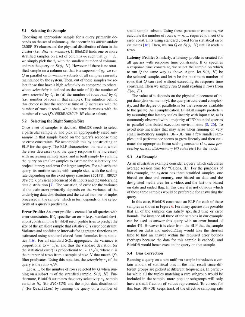
5.3 An ExampleAs an illustrative example consider a query which calculatesaverage session time for “Galena, IL”. For the purposes ofthis example, the system has three stratified samples, onebiased on date and country, one biased on date and thedesignated media area for a video, and the last one biasedon date and ended flag. In this case it is not obvious whichof these three samples would be preferable for answering thequery.

In this case, BlinkDB constructs an ELP for each of thesesamples as shown in Figure 6. For many queries it is possiblethat all of the samples can satisfy specified time or errorbounds. For instance all three of the samples in our examplecan be used to answer this query with an error bound ofunder 4%. However it is clear from the ELP that the samplebiased on date and ended flag would take the shortesttime to find an answer within the required error bounds(perhaps because the data for this sample is cached), andBlinkDB would hence execute the query on that sample.

5.4 Bias CorrectionRunning a query on a non-uniform sample introduces a cer-tain amount of statistical bias in the final result since dif-ferent groups are picked at different frequencies. In particu-lar while all the tuples matching a rare subgroup would beincluded in the sample, more popular subgroups will onlyhave a small fraction of values represented. To correct forthis bias, BlinkDB keeps track of the effective sampling rate

(a) dt, country

(b) dt, dma

(c) dt, ended flag

Figure 6. Error Latency Profiles for a variety of samples when executing a query to calculate average session time in Galena.(a) Shows the ELP for a sample biased on date and country, (b) is the ELP for a sample biased on date and designatedmedia area (dma), and (c) is the ELP for a sample biased on date and the ended flag.

Hadoop  Distributed  File  System  (HDFS)  

Spark  

Hadoop  MapReduce  

BlinkDB  Metastore  

Hive  Query  Engine  

Shark  (Hive  on  Spark)  

Sample  Creation  and    Maintenance  

BlinkDB  Query  Interface  

Sample  Selection  Uncertainty  Propagation  

Figure 7. BlinkDB’s Implementation Stack

for each group associated with each sample in a hidden col-umn as part of the sample table schema, and uses this toweight different subgroups to produce an unbiased result.

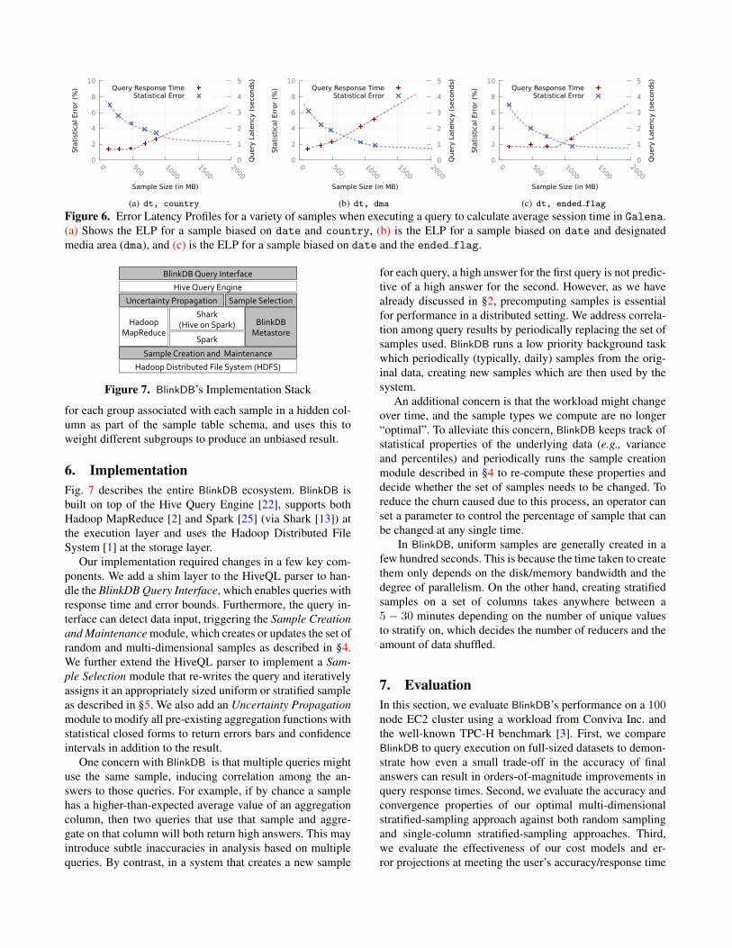
6. ImplementationFig. 7 describes the entire BlinkDB ecosystem. BlinkDB isbuilt on top of the Hive Query Engine [22], supports bothHadoop MapReduce [2] and Spark [25] (via Shark [13]) atthe execution layer and uses the Hadoop Distributed FileSystem [1] at the storage layer.

Our implementation required changes in a few key com-ponents. We add a shim layer to the HiveQL parser to han-dle the BlinkDB Query Interface, which enables queries withresponse time and error bounds. Furthermore, the query in-terface can detect data input, triggering the Sample Creationand Maintenance module, which creates or updates the set ofrandom and multi-dimensional samples as described in §4.We further extend the HiveQL parser to implement a Sam-ple Selection module that re-writes the query and iterativelyassigns it an appropriately sized uniform or stratified sampleas described in §5. We also add an Uncertainty Propagationmodule to modify all pre-existing aggregation functions withstatistical closed forms to return errors bars and confidenceintervals in addition to the result.

One concern with BlinkDB is that multiple queries mightuse the same sample, inducing correlation among the an-swers to those queries. For example, if by chance a samplehas a higher-than-expected average value of an aggregationcolumn, then two queries that use that sample and aggre-gate on that column will both return high answers. This mayintroduce subtle inaccuracies in analysis based on multiplequeries. By contrast, in a system that creates a new sample

for each query, a high answer for the first query is not predic-tive of a high answer for the second. However, as we havealready discussed in §2, precomputing samples is essentialfor performance in a distributed setting. We address correla-tion among query results by periodically replacing the set ofsamples used. BlinkDB runs a low priority background taskwhich periodically (typically, daily) samples from the orig-inal data, creating new samples which are then used by thesystem.

An additional concern is that the workload might changeover time, and the sample types we compute are no longer“optimal”. To alleviate this concern, BlinkDB keeps track ofstatistical properties of the underlying data (e.g., varianceand percentiles) and periodically runs the sample creationmodule described in §4 to re-compute these properties anddecide whether the set of samples needs to be changed. Toreduce the churn caused due to this process, an operator canset a parameter to control the percentage of sample that canbe changed at any single time.

In BlinkDB, uniform samples are generally created in afew hundred seconds. This is because the time taken to createthem only depends on the disk/memory bandwidth and thedegree of parallelism. On the other hand, creating stratifiedsamples on a set of columns takes anywhere between a5 − 30 minutes depending on the number of unique valuesto stratify on, which decides the number of reducers and theamount of data shuffled.

7. EvaluationIn this section, we evaluate BlinkDB’s performance on a 100node EC2 cluster using a workload from Conviva Inc. andthe well-known TPC-H benchmark [3]. First, we compareBlinkDB to query execution on full-sized datasets to demon-strate how even a small trade-off in the accuracy of finalanswers can result in orders-of-magnitude improvements inquery response times. Second, we evaluate the accuracy andconvergence properties of our optimal multi-dimensionalstratified-sampling approach against both random samplingand single-column stratified-sampling approaches. Third,we evaluate the effectiveness of our cost models and er-ror projections at meeting the user’s accuracy/response time

0 20 40 60 80

100 120 140 160 180 200

50% 100% 200%

Act

ual S

tora

ge C

ost

(%

)

Storage Budget (%)

[dt jointimems][objectid jointimems]

[dt dma]

[country endedflag][dt country]

[other columns]

(a) Biased Samples (Conviva)

0 20 40 60 80

100 120 140 160 180 200

50% 100% 200%

Act

ual S

tora

ge C

ost

(%

)

Storage Budget (%)

[orderkey suppkey][commitdt receiptdt]

[quantity]

[discount][shipmode]

[other columns]

(b) Biased Samples (TPC-H)

1

10

100

1000

10000

100000

2.5TB 7.5TB

Query

Serv

ice T

ime

(seco

nd

s)

Input Data Size (TB)

HiveHive on Spark (without caching)

Hive on Spark (with caching)BlinkDB (1% relative error)

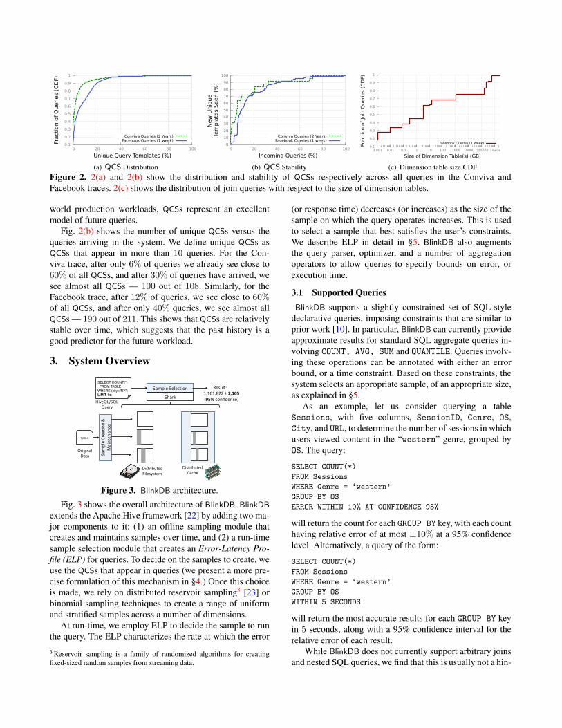
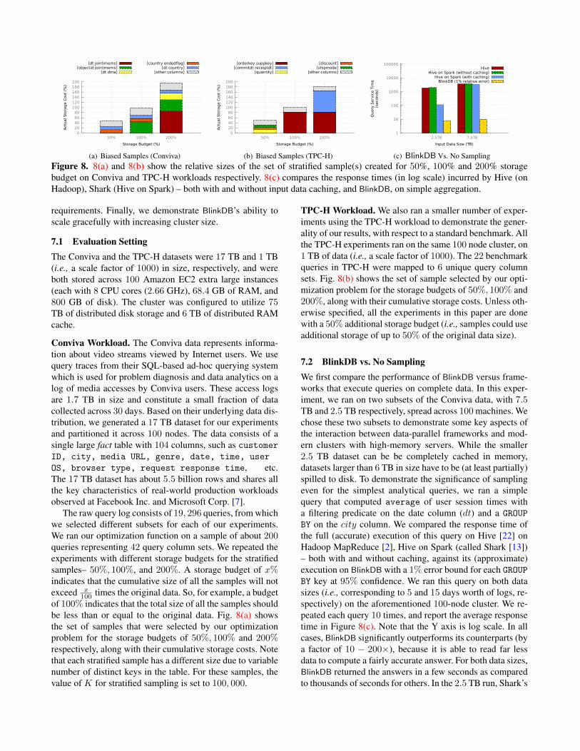
(c) BlinkDB Vs. No SamplingFigure 8. 8(a) and 8(b) show the relative sizes of the set of stratified sample(s) created for 50%, 100% and 200% storagebudget on Conviva and TPC-H workloads respectively. 8(c) compares the response times (in log scale) incurred by Hive (onHadoop), Shark (Hive on Spark) – both with and without input data caching, and BlinkDB, on simple aggregation.

requirements. Finally, we demonstrate BlinkDB’s ability toscale gracefully with increasing cluster size.

7.1 Evaluation SettingThe Conviva and the TPC-H datasets were 17 TB and 1 TB(i.e., a scale factor of 1000) in size, respectively, and wereboth stored across 100 Amazon EC2 extra large instances(each with 8 CPU cores (2.66 GHz), 68.4 GB of RAM, and800 GB of disk). The cluster was configured to utilize 75TB of distributed disk storage and 6 TB of distributed RAMcache.

Conviva Workload. The Conviva data represents informa-tion about video streams viewed by Internet users. We usequery traces from their SQL-based ad-hoc querying systemwhich is used for problem diagnosis and data analytics on alog of media accesses by Conviva users. These access logsare 1.7 TB in size and constitute a small fraction of datacollected across 30 days. Based on their underlying data dis-tribution, we generated a 17 TB dataset for our experimentsand partitioned it across 100 nodes. The data consists of asingle large fact table with 104 columns, such as customerID, city, media URL, genre, date, time, user

OS, browser type, request response time, etc.The 17 TB dataset has about 5.5 billion rows and shares allthe key characteristics of real-world production workloadsobserved at Facebook Inc. and Microsoft Corp. [7].

The raw query log consists of 19, 296 queries, from whichwe selected different subsets for each of our experiments.We ran our optimization function on a sample of about 200queries representing 42 query column sets. We repeated theexperiments with different storage budgets for the stratifiedsamples– 50%, 100%, and 200%. A storage budget of x%indicates that the cumulative size of all the samples will notexceed x

100 times the original data. So, for example, a budgetof 100% indicates that the total size of all the samples shouldbe less than or equal to the original data. Fig. 8(a) showsthe set of samples that were selected by our optimizationproblem for the storage budgets of 50%, 100% and 200%respectively, along with their cumulative storage costs. Notethat each stratified sample has a different size due to variablenumber of distinct keys in the table. For these samples, thevalue of K for stratified sampling is set to 100, 000.

TPC-H Workload. We also ran a smaller number of exper-iments using the TPC-H workload to demonstrate the gener-ality of our results, with respect to a standard benchmark. Allthe TPC-H experiments ran on the same 100 node cluster, on1 TB of data (i.e., a scale factor of 1000). The 22 benchmarkqueries in TPC-H were mapped to 6 unique query columnsets. Fig. 8(b) shows the set of sample selected by our opti-mization problem for the storage budgets of 50%, 100% and200%, along with their cumulative storage costs. Unless oth-erwise specified, all the experiments in this paper are donewith a 50% additional storage budget (i.e., samples could useadditional storage of up to 50% of the original data size).

7.2 BlinkDB vs. No SamplingWe first compare the performance of BlinkDB versus frame-works that execute queries on complete data. In this exper-iment, we ran on two subsets of the Conviva data, with 7.5TB and 2.5 TB respectively, spread across 100 machines. Wechose these two subsets to demonstrate some key aspects ofthe interaction between data-parallel frameworks and mod-ern clusters with high-memory servers. While the smaller2.5 TB dataset can be be completely cached in memory,datasets larger than 6 TB in size have to be (at least partially)spilled to disk. To demonstrate the significance of samplingeven for the simplest analytical queries, we ran a simplequery that computed average of user session times witha filtering predicate on the date column (dt) and a GROUP

BY on the city column. We compared the response time ofthe full (accurate) execution of this query on Hive [22] onHadoop MapReduce [2], Hive on Spark (called Shark [13])– both with and without caching, against its (approximate)execution on BlinkDB with a 1% error bound for each GROUP

BY key at 95% confidence. We ran this query on both datasizes (i.e., corresponding to 5 and 15 days worth of logs, re-spectively) on the aforementioned 100-node cluster. We re-peated each query 10 times, and report the average responsetime in Figure 8(c). Note that the Y axis is log scale. In allcases, BlinkDB significantly outperforms its counterparts (bya factor of 10 − 200×), because it is able to read far lessdata to compute a fairly accurate answer. For both data sizes,BlinkDB returned the answers in a few seconds as comparedto thousands of seconds for others. In the 2.5 TB run, Shark’s

caching capabilities help considerably, bringing the queryruntime down to about 112 seconds. However, with 7.5 TBof data, a considerable portion of data is spilled to disk andthe overall query response time is considerably longer.

7.3 Multi-Dimensional Stratified SamplingNext, we ran a set of experiments to evaluate the er-ror (§7.3.1) and convergence (§7.3.2) properties of our opti-mal multi-dimensional stratified-sampling approach againstboth simple random sampling, and one-dimensional strati-fied sampling (i.e., stratified samples over a single column).For these experiments we constructed three sets of sampleson both Conviva and TPC-H data with a 50% storage con-straint:

1. Uniform Samples. A sample containing 50% of theentire data, chosen uniformly at random.

2. Single-Dimensional Stratified Samples. The columnto stratify on was chosen using the same optimization frame-work, restricted so a sample is stratified on exactly 1 column.

3. Multi-Dimensional Stratified Samples. The sets ofcolumns to stratify on were chosen using BlinkDB’s opti-mization framework (§4.2), restricted so that samples couldbe stratified on no more than 3 columns (considering fouror more column combinations caused our optimizer to takemore than a minute to complete).

7.3.1 Error PropertiesIn order to illustrate the advantages of our multi-dimensionalstratified sampling strategy, we compared the average statis-tical error at 95% confidence while running a query for 10seconds over the three sets of samples, all of which wereconstrained to be of the same size.

For our evaluation using Conviva’s data we used a set of40 of the most popular queries (with 5 unique QCSs) and 17TB of uncompressed data on 100 nodes. We ran a similarset of experiments on the standard TPC-H queries (with 6unique QCSs). The queries we chose were on the lineitemtable, and were modified to conform with HiveQL syntax.

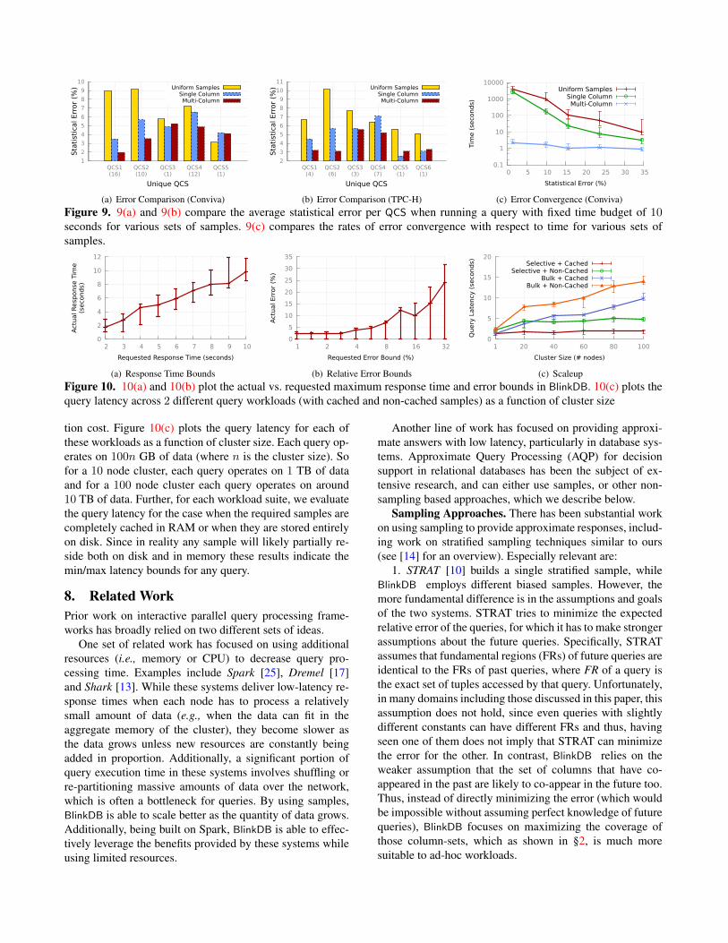
In Figures 9(a), and 9(b), we report the average statisti-cal error in the results of each of these queries when theyran on the aforementioned sets of samples. The queries arebinned according to the set(s) of columns in their GROUP BY,WHERE and HAVING clauses (i.e., their QCSs) and the num-bers in brackets indicate the number of queries which liein each bin. Based on the storage constraints, BlinkDB’s op-timization framework had samples stratified on QCS1 andQCS2 for Conviva data and samples stratified on QCS1,QCS2 and QCS4 for TPC-H data. For common QCSs,multi-dimensional samples produce smaller statistical errorsthan either one-dimensional or random samples. The opti-mization framework attempts to minimize expected error,rather than per-query errors, and therefore for some spe-cific QCS single-dimensional stratified samples behave bet-ter than multi-dimensional samples. Overall, however, our

optimization framework significantly improves performanceversus single column samples.

7.3.2 Convergence PropertiesWe also ran experiments to demonstrate the convergenceproperties of multi-dimensional stratified samples used byBlinkDB. We use the same set of three samples as §7.3, takenover 17 TB of Conviva data. Over this data, we ran multiplequeries to calculate average session time

For a particular ISP’s customers in 5 US Cities and deter-mined the latency for achieving a particular error bound with95% confidence. Results from this experiment (Figure 9(c))show that error bars from running queries over multi-dimensional samples converge orders-of-magnitude fasterthan random sampling (i.e., Hadoop Online [11, 19]), andare significantly faster to converge than single-dimensionalstratified samples.

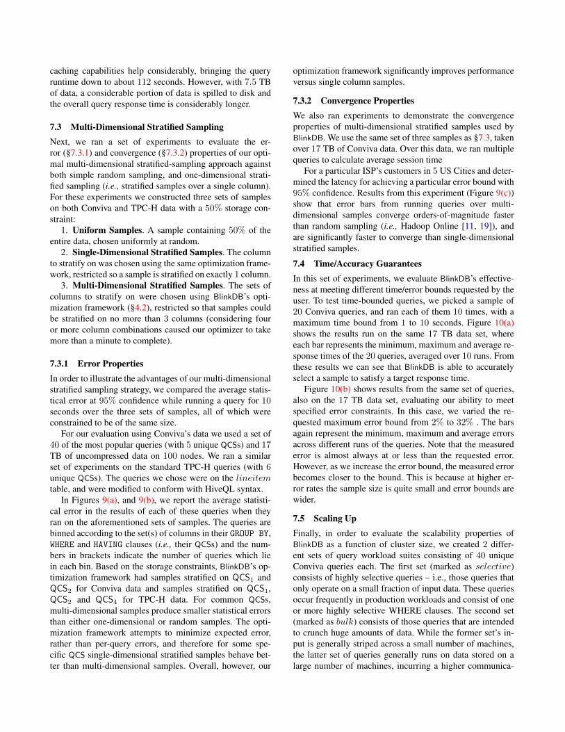
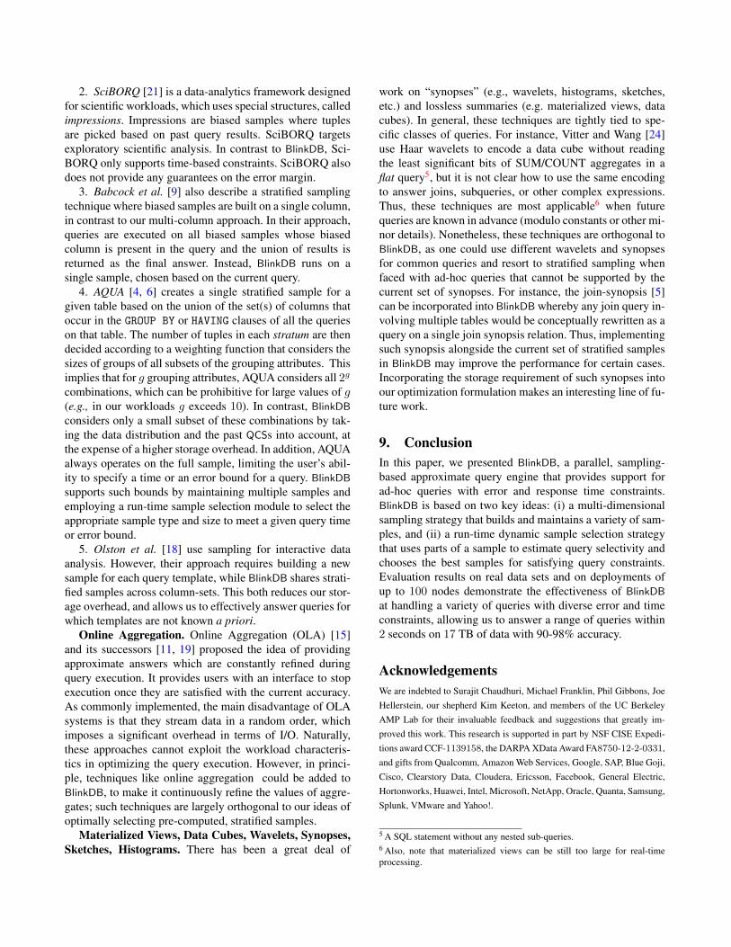
7.4 Time/Accuracy GuaranteesIn this set of experiments, we evaluate BlinkDB’s effective-ness at meeting different time/error bounds requested by theuser. To test time-bounded queries, we picked a sample of20 Conviva queries, and ran each of them 10 times, with amaximum time bound from 1 to 10 seconds. Figure 10(a)shows the results run on the same 17 TB data set, whereeach bar represents the minimum, maximum and average re-sponse times of the 20 queries, averaged over 10 runs. Fromthese results we can see that BlinkDB is able to accuratelyselect a sample to satisfy a target response time.

Figure 10(b) shows results from the same set of queries,also on the 17 TB data set, evaluating our ability to meetspecified error constraints. In this case, we varied the re-quested maximum error bound from 2% to 32% . The barsagain represent the minimum, maximum and average errorsacross different runs of the queries. Note that the measurederror is almost always at or less than the requested error.However, as we increase the error bound, the measured errorbecomes closer to the bound. This is because at higher er-ror rates the sample size is quite small and error bounds arewider.

7.5 Scaling UpFinally, in order to evaluate the scalability properties ofBlinkDB as a function of cluster size, we created 2 differ-ent sets of query workload suites consisting of 40 uniqueConviva queries each. The first set (marked as selective)consists of highly selective queries – i.e., those queries thatonly operate on a small fraction of input data. These queriesoccur frequently in production workloads and consist of oneor more highly selective WHERE clauses. The second set(marked as bulk) consists of those queries that are intendedto crunch huge amounts of data. While the former set’s in-put is generally striped across a small number of machines,the latter set of queries generally runs on data stored on alarge number of machines, incurring a higher communica-

1

2

3

4

5

6

7

8

9

10

QCS1(16)

QCS2(10)

QCS3(1)

QCS4(12)

QCS5(1)

Sta

tist

ical Err

or

(%)

Unique QCS

Uniform SamplesSingle ColumnMulti-Column

(a) Error Comparison (Conviva)

2

3

4

5

6

7

8

9

10

11

QCS1(4)

QCS2(6)

QCS3(3)

QCS4(7)

QCS5(1)

QCS6(1)

Sta

tist

ical Err

or

(%)

Unique QCS

Uniform SamplesSingle ColumnMulti-Column

(b) Error Comparison (TPC-H)

0.1

1

10

100

1000

10000

0 5 10 15 20 25 30 35

Tim

e (

seco

nds)

Statistical Error (%)

Uniform SamplesSingle ColumnMulti-Column

(c) Error Convergence (Conviva)Figure 9. 9(a) and 9(b) compare the average statistical error per QCS when running a query with fixed time budget of 10seconds for various sets of samples. 9(c) compares the rates of error convergence with respect to time for various sets ofsamples.

0

2

4

6

8

10

12

2 3 4 5 6 7 8 9 10

Act

ual R

esp

onse

Tim

e(s

eco

nds)

Requested Response Time (seconds)

(a) Response Time Bounds

0

5

10

15

20

25

30

35

1 2 4 8 16 32

Act

ual Err

or

(%)

Requested Error Bound (%)

(b) Relative Error Bounds

0

5

10

15

20

1 20 40 60 80 100

Query

Late

ncy

(se

conds)

Cluster Size (# nodes)

Selective + CachedSelective + Non-Cached

Bulk + CachedBulk + Non-Cached

(c) ScaleupFigure 10. 10(a) and 10(b) plot the actual vs. requested maximum response time and error bounds in BlinkDB. 10(c) plots thequery latency across 2 different query workloads (with cached and non-cached samples) as a function of cluster size

tion cost. Figure 10(c) plots the query latency for each ofthese workloads as a function of cluster size. Each query op-erates on 100n GB of data (where n is the cluster size). Sofor a 10 node cluster, each query operates on 1 TB of dataand for a 100 node cluster each query operates on around10 TB of data. Further, for each workload suite, we evaluatethe query latency for the case when the required samples arecompletely cached in RAM or when they are stored entirelyon disk. Since in reality any sample will likely partially re-side both on disk and in memory these results indicate themin/max latency bounds for any query.

8. Related WorkPrior work on interactive parallel query processing frame-works has broadly relied on two different sets of ideas.

One set of related work has focused on using additionalresources (i.e., memory or CPU) to decrease query pro-cessing time. Examples include Spark [25], Dremel [17]and Shark [13]. While these systems deliver low-latency re-sponse times when each node has to process a relativelysmall amount of data (e.g., when the data can fit in theaggregate memory of the cluster), they become slower asthe data grows unless new resources are constantly beingadded in proportion. Additionally, a significant portion ofquery execution time in these systems involves shuffling orre-partitioning massive amounts of data over the network,which is often a bottleneck for queries. By using samples,BlinkDB is able to scale better as the quantity of data grows.Additionally, being built on Spark, BlinkDB is able to effec-tively leverage the benefits provided by these systems whileusing limited resources.

Another line of work has focused on providing approxi-mate answers with low latency, particularly in database sys-tems. Approximate Query Processing (AQP) for decisionsupport in relational databases has been the subject of ex-tensive research, and can either use samples, or other non-sampling based approaches, which we describe below.

Sampling Approaches. There has been substantial workon using sampling to provide approximate responses, includ-ing work on stratified sampling techniques similar to ours(see [14] for an overview). Especially relevant are:

1. STRAT [10] builds a single stratified sample, whileBlinkDB employs different biased samples. However, themore fundamental difference is in the assumptions and goalsof the two systems. STRAT tries to minimize the expectedrelative error of the queries, for which it has to make strongerassumptions about the future queries. Specifically, STRATassumes that fundamental regions (FRs) of future queries areidentical to the FRs of past queries, where FR of a query isthe exact set of tuples accessed by that query. Unfortunately,in many domains including those discussed in this paper, thisassumption does not hold, since even queries with slightlydifferent constants can have different FRs and thus, havingseen one of them does not imply that STRAT can minimizethe error for the other. In contrast, BlinkDB relies on theweaker assumption that the set of columns that have co-appeared in the past are likely to co-appear in the future too.Thus, instead of directly minimizing the error (which wouldbe impossible without assuming perfect knowledge of futurequeries), BlinkDB focuses on maximizing the coverage ofthose column-sets, which as shown in §2, is much moresuitable to ad-hoc workloads.

2. SciBORQ [21] is a data-analytics framework designedfor scientific workloads, which uses special structures, calledimpressions. Impressions are biased samples where tuplesare picked based on past query results. SciBORQ targetsexploratory scientific analysis. In contrast to BlinkDB, Sci-BORQ only supports time-based constraints. SciBORQ alsodoes not provide any guarantees on the error margin.

3. Babcock et al. [9] also describe a stratified samplingtechnique where biased samples are built on a single column,in contrast to our multi-column approach. In their approach,queries are executed on all biased samples whose biasedcolumn is present in the query and the union of results isreturned as the final answer. Instead, BlinkDB runs on asingle sample, chosen based on the current query.

4. AQUA [4, 6] creates a single stratified sample for agiven table based on the union of the set(s) of columns thatoccur in the GROUP BY or HAVING clauses of all the querieson that table. The number of tuples in each stratum are thendecided according to a weighting function that considers thesizes of groups of all subsets of the grouping attributes. Thisimplies that for g grouping attributes, AQUA considers all 2g

combinations, which can be prohibitive for large values of g(e.g., in our workloads g exceeds 10). In contrast, BlinkDBconsiders only a small subset of these combinations by tak-ing the data distribution and the past QCSs into account, atthe expense of a higher storage overhead. In addition, AQUAalways operates on the full sample, limiting the user’s abil-ity to specify a time or an error bound for a query. BlinkDBsupports such bounds by maintaining multiple samples andemploying a run-time sample selection module to select theappropriate sample type and size to meet a given query timeor error bound.

5. Olston et al. [18] use sampling for interactive dataanalysis. However, their approach requires building a newsample for each query template, while BlinkDB shares strati-fied samples across column-sets. This both reduces our stor-age overhead, and allows us to effectively answer queries forwhich templates are not known a priori.

Online Aggregation. Online Aggregation (OLA) [15]and its successors [11, 19] proposed the idea of providingapproximate answers which are constantly refined duringquery execution. It provides users with an interface to stopexecution once they are satisfied with the current accuracy.As commonly implemented, the main disadvantage of OLAsystems is that they stream data in a random order, whichimposes a significant overhead in terms of I/O. Naturally,these approaches cannot exploit the workload characteris-tics in optimizing the query execution. However, in princi-ple, techniques like online aggregation could be added toBlinkDB, to make it continuously refine the values of aggre-gates; such techniques are largely orthogonal to our ideas ofoptimally selecting pre-computed, stratified samples.

Materialized Views, Data Cubes, Wavelets, Synopses,Sketches, Histograms. There has been a great deal of

work on “synopses” (e.g., wavelets, histograms, sketches,etc.) and lossless summaries (e.g. materialized views, datacubes). In general, these techniques are tightly tied to spe-cific classes of queries. For instance, Vitter and Wang [24]use Haar wavelets to encode a data cube without readingthe least significant bits of SUM/COUNT aggregates in aflat query5, but it is not clear how to use the same encodingto answer joins, subqueries, or other complex expressions.Thus, these techniques are most applicable6 when futurequeries are known in advance (modulo constants or other mi-nor details). Nonetheless, these techniques are orthogonal toBlinkDB, as one could use different wavelets and synopsesfor common queries and resort to stratified sampling whenfaced with ad-hoc queries that cannot be supported by thecurrent set of synopses. For instance, the join-synopsis [5]can be incorporated into BlinkDB whereby any join query in-volving multiple tables would be conceptually rewritten as aquery on a single join synopsis relation. Thus, implementingsuch synopsis alongside the current set of stratified samplesin BlinkDB may improve the performance for certain cases.Incorporating the storage requirement of such synopses intoour optimization formulation makes an interesting line of fu-ture work.

9. ConclusionIn this paper, we presented BlinkDB, a parallel, sampling-based approximate query engine that provides support forad-hoc queries with error and response time constraints.BlinkDB is based on two key ideas: (i) a multi-dimensionalsampling strategy that builds and maintains a variety of sam-ples, and (ii) a run-time dynamic sample selection strategythat uses parts of a sample to estimate query selectivity andchooses the best samples for satisfying query constraints.Evaluation results on real data sets and on deployments ofup to 100 nodes demonstrate the effectiveness of BlinkDB

at handling a variety of queries with diverse error and timeconstraints, allowing us to answer a range of queries within2 seconds on 17 TB of data with 90-98% accuracy.

AcknowledgementsWe are indebted to Surajit Chaudhuri, Michael Franklin, Phil Gibbons, JoeHellerstein, our shepherd Kim Keeton, and members of the UC BerkeleyAMP Lab for their invaluable feedback and suggestions that greatly im-proved this work. This research is supported in part by NSF CISE Expedi-tions award CCF-1139158, the DARPA XData Award FA8750-12-2-0331,and gifts from Qualcomm, Amazon Web Services, Google, SAP, Blue Goji,Cisco, Clearstory Data, Cloudera, Ericsson, Facebook, General Electric,Hortonworks, Huawei, Intel, Microsoft, NetApp, Oracle, Quanta, Samsung,Splunk, VMware and Yahoo!.

5 A SQL statement without any nested sub-queries.6 Also, note that materialized views can be still too large for real-timeprocessing.

References[1] Apache Hadoop Distributed File System. http://hadoop.apache.org/

hdfs/.[2] Apache Hadoop Mapreduce Project. http://hadoop.apache.org/

mapreduce/.[3] TPC-H Query Processing Benchmarks. http://www.tpc.org/tpch/.[4] S. Acharya, P. B. Gibbons, and V. Poosala. Congressional samples for approxi-

mate answering of group-by queries. In ACM SIGMOD, May 2000.[5] S. Acharya, P. B. Gibbons, V. Poosala, and S. Ramaswamy. Join synopses for

approximate query answering. In ACM SIGMOD, June 1999.[6] S. Acharya, P. B. Gibbons, V. Poosala, and S. Ramaswamy. The Aqua approxi-

mate query answering system. ACM SIGMOD Record, 28(2), 1999.[7] S. Agarwal, S. Kandula, N. Bruno, M.-C. Wu, I. Stoica, and J. Zhou. Re-

optimizing Data Parallel Computing. In NSDI, 2012.[8] G. Ananthanarayanan, S. Kandula, A. G. Greenberg, I. Stoica, and y. . . p. . . e.

. h. b. . D. others title = Reining in the Outliers in Map-Reduce Clusters usingMantri, booktitle = OSDI.

[9] B. Babcock, S. Chaudhuri, and G. Das. Dynamic sample selection for approxi-mate query processing. In VLDB, 2003.

[10] S. Chaudhuri, G. Das, and V. Narasayya. Optimized stratified sampling forapproximate query processing. TODS, 2007.

[11] T. Condie, N. Conway, P. Alvaro, J. M. Hellerstein, K. Elmeleegy, and R. Sears.Mapreduce online. In NSDI, 2010.

[12] G. Cormode. Sketch techniques for massive data. In Synposes for Massive Data:Samples, Histograms, Wavelets and Sketches. 2011.

[13] C. Engle, A. Lupher, R. Xin, M. Zaharia, et al. Shark: Fast Data Analysis UsingCoarse-grained Distributed Memory. In SIGMOD, 2012.

[14] M. Garofalakis and P. Gibbons. Approximate query processing: Taming theterabytes. In VLDB, 2001. Tutorial.

[15] J. M. Hellerstein, P. J. Haas, and H. J. Wang. Online aggregation. In SIGMOD,1997.

[16] S. Lohr. Sampling: design and analysis. Thomson, 2009.[17] S. Melnik, A. Gubarev, J. J. Long, G. Romer, S. Shivakumar, M. Tolton, and

T. Vassilakis. Dremel: interactive analysis of web-scale datasets. Commun. ACM,54:114–123, June 2011.

[18] C. Olston, E. Bortnikov, K. Elmeleegy, F. Junqueira, and B. Reed. Interactiveanalysis of web-scale data. In CIDR, 2009.

[19] N. Pansare, V. R. Borkar, C. Jermaine, and T. Condie. Online Aggregation forLarge MapReduce Jobs. PVLDB, 4(11):1135–1145, 2011.

[20] C. Sapia. Promise: Predicting query behavior to enable predictive cachingstrategies for olap systems. DaWaK, pages 224–233. Springer-Verlag, 2000.

[21] L. Sidirourgos, M. L. Kersten, and P. A. Boncz. SciBORQ: Scientific datamanagement with Bounds On Runtime and Quality. In CIDR’11, 2011.

[22] A. Thusoo, J. S. Sarma, N. Jain, et al. Hive: a warehousing solution over a map-reduce framework. PVLDB, 2(2), 2009.

[23] S. Tirthapura and D. Woodruff. Optimal random sampling from distributedstreams revisited. Distributed Computing, pages 283–297, 2011.

[24] J. S. Vitter and M. Wang. Approximate computation of multidimensional aggre-gates of sparse data using wavelets. SIGMOD, 1999.

[25] M. Zaharia et al. Resilient distributed datasets: A fault-tolerant abstraction forin-memory cluster computing. In NSDI, 2012.

[26] M. Zaharia, A. Konwinski, A. D. Joseph, et al. Improving MapReduce Perfor-mance in Heterogeneous Environments. In OSDI, 2008.