improved modeling of three-point estimates for decision
TRANSCRIPT
Calhoun: The NPS Institutional Archive
Theses and Dissertations Thesis and Dissertation Collection
2016-03
Improved modeling of three-point estimates for
decision making: going beyond the triangle
Mulligan, Daniel W.
Monterey, California: Naval Postgraduate School
http://hdl.handle.net/10945/48571

NAVAL POSTGRADUATE
SCHOOL
MONTEREY, CALIFORNIA
THESIS
Approved for public release; distribution is unlimited
IMPROVED MODELING OF THREE-POINT ESTIMATES FOR DECISION MAKING: GOING
BEYOND THE TRIANGLE
by
Daniel W. Mulligan
March 2016
Thesis Advisor: Mark Rhoades Second Reader: Walter Owen

THIS PAGE INTENTIONALLY LEFT BLANK

i
REPORT DOCUMENTATION PAGE Form Approved OMB No. 0704–0188
Public reporting burden for this collection of information is estimated to average 1 hour per response, including the time for reviewing instruction, searching existing data sources, gathering and maintaining the data needed, and completing and reviewing the collection of information. Send comments regarding this burden estimate or any other aspect of this collection of information, including suggestions for reducing this burden, to Washington headquarters Services, Directorate for Information Operations and Reports, 1215 Jefferson Davis Highway, Suite 1204, Arlington, VA 22202-4302, and to the Office of Management and Budget, Paperwork Reduction Project (0704-0188) Washington, DC 20503. 1. AGENCY USE ONLY (Leave blank)
2. REPORT DATE March 2016
3. REPORT TYPE AND DATES COVERED Master’s thesis
4. TITLE AND SUBTITLE IMPROVED MODELING OF THREE-POINT ESTIMATES FOR DECISION MAKING: GOING BEYOND THE TRIANGLE
5. FUNDING NUMBERS
6. AUTHOR(S) Daniel W. Mulligan 7. PERFORMING ORGANIZATION NAME(S) AND ADDRESS(ES)
Naval Postgraduate School Monterey, CA 93943-5000
8. PERFORMING ORGANIZATION REPORT NUMBER
9. SPONSORING /MONITORING AGENCY NAME(S) AND ADDRESS(ES)
N/A
10. SPONSORING / MONITORING AGENCY REPORT NUMBER
11. SUPPLEMENTARY NOTES The views expressed in this thesis are those of the author and do not reflect the official policy or position of the Department of Defense or the U.S. Government. IRB Protocol number ____N/A____. 12a. DISTRIBUTION / AVAILABILITY STATEMENT Approved for public release; distribution is unlimited
12b. DISTRIBUTION CODE
13. ABSTRACT (maximum 200 words) Decision making in engineering development projects and programs relies on numbers. This
quantitative support can involve uncertainty that is frequently characterized by three-point estimates of decision variables. Modeling of these estimates for analysis commonly utilizes the triangular distribution for its simplicity, but errors could be introduced if another distribution model is more appropriate for the data. This study measures statistics from distribution types ranging from fully flat to narrowly peaked, fitting estimates for all sizes of minimum to maximum ranges and spanning the complete spectrum of asymmetry. The study compares common statistical values for each distribution to an equivalent triangular distribution. It calculates the error size for the mean, high-confidence interval, and coefficient of variation. The study then provides recommendations for when to use a triangular distribution or a different model. The guidelines are based on a weight factor of the distribution mode and the estimate’s maturity to produce an objective set of guidelines for selecting distribution shapes best suited to model any given three-point estimate. With these guidelines, estimators and modelers can quickly and easily provide a more accurate uncertainty analysis to support decision makers.
14. SUBJECT TERMS project management, program management, systems engineering, decision making, uncertainty, uncertainty modeling, three-point estimate, triangular distribution, probability distribution, mode weight
15. NUMBER OF PAGES
91 16. PRICE CODE
17. SECURITY CLASSIFICATION OF REPORT
Unclassified
18. SECURITY CLASSIFICATION OF THIS PAGE
Unclassified
19. SECURITY CLASSIFICATION OF ABSTRACT
Unclassified
20. LIMITATION OF ABSTRACT
UU NSN 7540–01-280-5500 Standard Form 298 (Rev. 2–89) Prescribed by ANSI Std. 239–18

ii
THIS PAGE INTENTIONALLY LEFT BLANK

iii
Approved for public release; distribution is unlimited
IMPROVED MODELING OF THREE-POINT ESTIMATES FOR DECISION MAKING: GOING BEYOND THE TRIANGLE
Daniel W. Mulligan Civilian, National Aeronautics and Space Administration
B.S., United States Naval Academy, 1988
Submitted in partial fulfillment of the requirements for the degree of
MASTER OF SCIENCE IN SYSTEMS ENGINEERING MANAGEMENT
from the
NAVAL POSTGRADUATE SCHOOL March 2016
Approved by: Mark Rhoades Thesis Advisor
Walter Owen, DPA Second Reader
Ronald Giachetti, Ph.D. Chair, Department of Systems Engineering

iv
THIS PAGE INTENTIONALLY LEFT BLANK

v
ABSTRACT
Decision making in engineering development projects and programs relies on
numbers. This quantitative support can involve uncertainty that is frequently
characterized by three-point estimates of decision variables. Modeling of these estimates
for analysis commonly utilizes the triangular distribution for its simplicity, but errors
could be introduced if another distribution model is more appropriate for the data. This
study measures statistics from distribution types ranging from fully flat to narrowly
peaked, fitting estimates for all sizes of minimum to maximum ranges and spanning the
complete spectrum of asymmetry. The study compares common statistical values for each
distribution to an equivalent triangular distribution. It calculates the error size for the
mean, high-confidence interval, and coefficient of variation. The study then provides
recommendations for when to use a triangular distribution or a different model. The
guidelines are based on a weight factor of the distribution mode and the estimate’s
maturity to produce an objective set of guidelines for selecting distribution shapes best
suited to model any given three-point estimate. With these guidelines, estimators and
modelers can quickly and easily provide a more accurate uncertainty analysis to support
decision makers.

vi
THIS PAGE INTENTIONALLY LEFT BLANK

vii
TABLE OF CONTENTS
I. INTRODUCTION..................................................................................................1 A. BACKGROUND: DECISION MAKING WITH THREE-
POINT ESTIMATES.................................................................................1 B. RESEARCH QUESTIONS: POTENTIAL ERROR IN
COMMON PRACTICE ............................................................................9 C. METHODOLOGY: COMPARING DISTRIBUTION
STATISTICS ............................................................................................10
II. STUDY OF TRIANGULAR DISTRIBUTION VERSUS OTHER TYPES OF DISTRIBUTIONS ...........................................................................13 A. DISTRIBUTION AND DECISION VARIABLE
FRAMEWORK ........................................................................................13 B. FOUR REPRESENTATIVE NOTIONAL CASES ..............................17 C. REPRESENTATIVE DISTRIBUTIONS ..............................................19 D. ANALYSIS OF DECISION VARIABLE VALUES .............................29
1. By Estimate Case..........................................................................29 2. By Decision Variable....................................................................39
III. SELECTION OF ALTERNATIVE DISTRIBUTION TYPES .......................47 A. QUALITATIVE RELATIONSHIPS OF DISTRIBUTIONS ..............47 B. VISUAL SURVEY ...................................................................................47 C. QUALITATIVE MODE WEIGHT........................................................49 D. QUANTITATIVE MODE WEIGHT .....................................................50 E. PRACTICAL APPLICATION ...............................................................54
IV. CONCLUSION ....................................................................................................63 A. OBJECTIVE GUIDELINES FOR USE OF TRIANGULAR
DISTRIBUTION OR OTHER DISTRIBUTION .................................63 B. SUBJECTIVE AND OBJECTIVE GUIDELINES FOR
DISTRIBUTION SELECTION ..............................................................64
APPENDIX: DISTRIBUTION EQUATIONS ..............................................................67
LIST OF REFERENCES ................................................................................................69
INITIAL DISTRIBUTION LIST ...................................................................................71

viii
THIS PAGE INTENTIONALLY LEFT BLANK

ix
LIST OF FIGURES
Figure 1. Subjective Uncertainty Boundary Interpretation and Tail Extension for 70% Confidence Interval Applied to Subject Matter Expert Elicitation. ....................................................................................................5
Figure 2. Common Triangular Distribution Model of a Three-Point Estimate, with Probability Density Function and Cumulative Distribution Function. ......................................................................................................6
Figure 3. Common Probability Distributions Used in Uncertainty Analysis. .............8
Figure 4. Common Triangular Distribution Model of a Scaled Three-Point Estimate, with Probability Density Function and Cumulative Distribution Function. ................................................................................14
Figure 5. Scaled Distribution High-Confidence Point Cumulative Probability as Function of Asymmetry. ........................................................................17
Figure 6. Boundary Distribution Choices for Scaled Case A′. ..................................22
Figure 7. Representative Distribution Model PDFs for Scaled Three-Point Estimate Case A′ = [0,0.5,1.0]. ..................................................................23
Figure 8. Examples of Constrained Beta-n Distribution at Various Degrees of Asymmetry. ................................................................................................25
Figure 9. Examples of Constrained Beta-o Distribution at Various Degrees of Asymmetry. ................................................................................................26
Figure 10. Representative Distribution Model PDFs for Scaled Three-Point Estimate Case B′ = [0,0.33,1.0]. ................................................................27
Figure 11. Representative Distribution Model PDFs for Scaled Three-Point Estimate Case C′ = [0,0.125,1.0]. ..............................................................28
Figure 12. Representative Distribution Model PDFs for Scaled Three-Point Estimate Case D′ = [0,0,1.0]. .....................................................................29
Figure 13. Case A High-Confidence Point Base Unit Difference from Triangular as a Function of Range Magnitude Proportion. .......................33
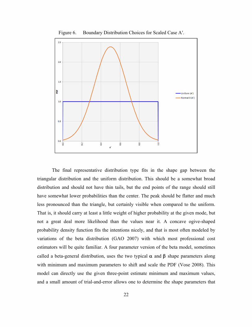
Figure 14. Case A High-Confidence Point Base Unit Difference from Triangular as a Function of Range Magnitude Proportion (Lognormal). ..............................................................................................34
Figure 15. Scaled Distribution Mean Shift as a Function of Asymmetry. ..................40
Figure 16. Scaled Distribution Mean Difference from Triangular Mean as a Function of Asymmetry. ............................................................................40
Figure 17. Scaled Distribution SD Shift as a Function of Asymmetry. ......................42

x
Figure 18. Scaled Distribution High-Confidence Point Shift as a Function of Asymmetry. ................................................................................................42
Figure 19. Scaled Distribution High-Confidence Point Difference From Triangular as a Function of Asymmetry. ...................................................43
Figure 20. Scaled Distribution Coefficient of Variation Shift as a Function of Asymmetry. ................................................................................................44
Figure 21. Scaled Distribution Coefficient of Variation Difference from Triangular as a Function of Asymmetry. ...................................................45
Figure 22. Representative Distribution Model PDFs for Scaled Three-Point Estimate Case A′ = [0,0.5,1.0]. ..................................................................48
Figure 23. Benefit-to-Cost (B/C) Ratio of Options for Design Down-Selection Decision Using High-Confidence Value from Triangular Modeling of Uncertainty. ...........................................................................................57
Figure 24. Cost as an Independent Variable (CAIV) Plot for Design Down-Selection Decision Using High-Confidence Value from Triangular Modeling of Uncertainty. ...........................................................................57
Figure 25. Benefit-to-Cost (B/C) Ratio of Options for Design Down-Selection Decision Using High-Confidence Value from Beta Modeling of Uncertainty. ................................................................................................60
Figure 26. Cost as an Independent Variable (CAIV) Plot for Design Down-Selection Decision Using High-Confidence Value from Beta Modeling of Uncertainty. ...........................................................................61

xi
LIST OF TABLES
Table 1. Case A′ Statistical and Comparison Data. .................................................30
Table 2. Case B′ Statistical and Comparison Data. ..................................................35
Table 3. Case C′ Statistical and Comparison Data. ..................................................37
Table 4. Case D′ Statistical and Comparison Data. .................................................38
Table 5. Three-point Estimates For Design Down-Selection Decision Figures of Merit, and High-Confidence Value From Triangular Modeling of Uncertainty. ................................................................................................55
Table 6. Multiple Attribute Decision-Making Analysis for Design Down-Selection Decision Using High-Confidence Value from Triangular Modeling of Uncertainty. ...........................................................................56
Table 7. Three-Point Estimates for Design Down-Selection Decision Figures of Merit, and High-Confidence Value from Beta Distribution Modeling of Uncertainty. ...........................................................................59
Table 8. Multiple Attribute Decision-Making Analysis for Design Down-Selection Decision Using High-Confidence Value from Beta Modeling of Uncertainty. ...........................................................................60
Table 9. Objective Guidelines for Use of Triangular Distribution or Other Distribution. ...............................................................................................64
Table 10. Subjective and Objective Guidelines for Distribution Selection. ..............65

xii
THIS PAGE INTENTIONALLY LEFT BLANK

xiii
LIST OF ACRONYMS AND ABBREVIATIONS
AF CRUH Air Force Cost Risk and Uncertainty Handbook
AIE Applied Information Economics
AoA Analysis of alternatives
B/C Benefit-to-cost ratio
CAIV Cost as an independent variable
CBA Cost-benefit analysis
CDF Cumulative distribution function
CER Cost estimating relationship
CI Confidence interval
CRA Cost risk analysis
CV Coefficient of variation
FMEA Failure modes and effects analysis
FOM Figure of merit
GAO Government Accountability Office
JCL Joint confidence level
MADM Multiple attribute decision making
MOE Measure of effectiveness
MOP Measure of performance
NPV Net present value
PDF Probability density function
PMBOK Project Management Body of Knowledge
PRA Probabilistic risk assessment
ROM Rough order of magnitude
SD Standard deviation
SME Subject matter expert
SRA Schedule risk analysis
UMDO Uncertainty-based multidisciplinary design optimization

xiv
THIS PAGE INTENTIONALLY LEFT BLANK

xv
EXECUTIVE SUMMARY
Decisions in development programs for large complex systems, such as major
weapon systems or spacecraft, are inevitably made under uncertainty. New applications
of technology and first-time work approaches mean that very little direct evidence of past
performance, either technical or programmatic, will be available to support planning
decisions that are crucial to the success of the program. Estimates of the cost of scope to
be performed and work activity durations are especially vulnerable to uncertainty due to
inexact relationships to previously executed tasks. Even technical measures sometimes
have large unknowns or undefined content that still require quantification for engineering
use in design, performance and environment parameters.
When uncertain estimates with a subjective basis are used, they typically take the
form of a three-point estimate. These estimates are usually generated by eliciting the
opinions of subject matter experts, who in their best judgment provide a best case, worst
case, and most likely quantitative estimate for the value in question. Common practice for
quantitatively analyzing the uncertainty of the given three-point estimate is the use of a
triangular distribution model to provide for probabilistic and statistical handling of an
estimate.
While explicit characterization of the estimate uncertainty is a best practice,
inattentive default use of the simple triangle model can introduce significant error in
some infrequent conditions, when the estimate data supports the modeling of a different
and more appropriate type of distribution. This study does not focus on areas where
analysts have significant objective sample data available leading to explicit objective
distribution models for use, and it does not address maturity of elicitation techniques for
subjective estimating that might correct for biases by adjusting the values of a three-point
estimate. Instead, the purpose of this study is to examine the specific case when a
subjective three-point estimate is provided and the data is modeled as-is for use in
decision making. This examination allows for measurement of the potential error possible
in the common practice of using a triangle model to represent the three-point estimate.
The study also recommends alternative solutions to minimize this error. This measurable

xvi
error can be predicted from observation of the given three-point estimate data, and
countered with simple selection of alternative distribution model types for uncertainty
analysis. Simple guidelines with objective indicators to identify vulnerable estimate
conditions and to support alternative distribution selections are developed as results
herein.
In this study, measurement of error size is conducted by comparison of the
common statistical values of mean and standard deviation (SD) as they apply to use in
decision variables. The error size is calculated for multiple estimate cases varying in
asymmetry and minimum to maximum range, each modeled by multiple possible
distribution choices fit to the three-point estimate values. The study provides tabulation
of differences for each distribution’s statistical values versus the equivalent values for a
matching triangular distribution, and identifies ranges of error magnitude possible for
each estimate case. It also provides graphical display of values for all estimate cases that
extend the point observations of each case into general findings.
This study develops an objective method to help choose an appropriate model in
the cases where a distribution selection other than the default triangle model should be
used. It also examines a mode weight factor that applies to the shape and scale of the
typical alternative distributions. Quantifying this factor and using it in a derivation of
parameters of a customized beta distribution relates it exactly to statistical measures of
each type of typical distribution. Association of the values of this mode weight factor
with qualitative scales of subject matter expert elicitation confidence or basis of estimate
maturity lead to an intuitive score that points objectively to a distribution choice with
matching shape and scale.
The results of this study culminate in two simple guideline tables. The first
generalizes the regions of three-point estimate cases where triangles are safe from
significant error. These regions occur in combinations of near-symmetrical estimate
values, small relative minimum to maximum range magnitude and medium basis of
estimate maturity are found. This table also indicates less frequent conditions where
three-point estimates are vulnerable to error, thereby recommending a model choice other
than triangle. The second guideline table utilizes a simple five-point qualitative scale

xvii
related to either a degree of subjective confidence in the mode of an elicited three-point
estimate, or a measure of the maturity of the basis of the given estimate. The scale then
matches those scores to typical distributions suggested by an appropriate corresponding
mode weight.
This research benefits modelers conducting uncertainty analysis by providing
improved repeatability, accuracy and credibility of analytical results without sacrificing
agility or simplicity. It also benefits managers who structure quantitatively based decision
analyses, who will find increased rigor in the handling of data inputs and have more
explicit and complete use of available data. Decision makers will have the most accurate
data that best represents known states of uncertainty, with avoidance of hidden risks or
situations of decision reversal as a result.

xviii
THIS PAGE INTENTIONALLY LEFT BLANK

1
I. INTRODUCTION
A. BACKGROUND: DECISION MAKING WITH THREE-POINT ESTIMATES
All project and program managers are inevitably faced with situations where they
are called upon to make decisions with only uncertain information available to support
the basis of their choices. This is especially true in complex engineering development
projects, such as spacecraft and major weapon systems, where cutting-edge technologies
meet first-use cases and once state-of-the-art heritage systems are modified for new
applications, with little directly analogous data upon which to draw. Explicit
characterization of uncertainty is preferred in such cases since “the superiority of even
simple quantitative models for decision making has been established for many areas
normally thought to be the preserve of expert intuition” (Hubbard 2014, 8).
Most engineering analyses will utilize objectively determined uncertainty, where
statistically significant amounts of measured data provide full definition of the range and
distribution of values of a particular quantity of interest. Still, there are numerous
analyses that support decisions throughout the entire systems engineering life cycle that
rely on subjective uncertainty to enable actionable results. Several key examples are
drawn from general life cycle process descriptions in the NASA Systems Engineering
Handbook and paraphrased in the following paragraphs.
From the earliest stages of pre-formulation, capability engineering portfolios and
feasibility studies utilize quantified Pareto optimality and cost as an independent variable
(CAIV) analyses. These analyses can determine system capabilities or scope to pursue in
a development program. The effects of uncertainty on capability estimates can alter the
position of specific content on or relative to an efficient frontier, and therefore effect
whether those capabilities are included in development or not. Prior to acquisition and
contracting for a system, values of subjective estimates often provide boundary data for
simulation and use case development that support acquisition strategies.

2
While developing system requirements, initial estimates of expected performance
and quality measures are determined. These aid in determining measures of effectiveness
(MOE), and measures of performance (MOP) that have realistic threshold and objective
values. Requirements-based parametric cost estimates early in the life cycle for proposed
systems frequently rely upon subjective uncertainty of technical parameter inputs to cost
estimating relationship (CER) models. Analysis of alternatives (AoA) models utilizing
multiple criteria decision-making techniques are fundamental to selection of technical
solutions for a system. These strategic decisions precede the move into the design phases
of a program, and can be strongly influenced by uncertain estimates.
In design and analysis cycles, engineering trade studies might use subjective
component performance estimates to prune unfavorable configurations from further
detailed study. Specific configuration selections often rely on cost-benefit analyses that
can be sensitive to estimating uncertainty. Prior to detailed failure modes and effects
analyses (FMEA), preliminary quantification of risk probabilities and severity influence
reliability requirements and approaches in preliminary design. Detailed design discipline
may involve uncertainty-based multidisciplinary design optimization (UMDO) methods
effective under measured objective uncertainty but can utilize subjective uncertainty
inputs when needed.
Initial build-up or bottom-up cost estimates often require subjective estimation of
their cost model inputs to enable aggregate program cost risk analysis (CRA) to
accompany milestone design reviews. Schedule logic network tasks tend to rely on
subjective estimates of durations that affect critical path determinations and schedule risk
analysis (SRA), and coupled CRA-SRA analyses provide for joint confidence level (JCL)
evaluations required for authorization of major government development programs.
Expert elicitation of extremely remote and unobserved failure rates is often
needed in system safety probabilistic risk assessment (PRA) to determine aggregate
probability of loss of mission or loss of system. In manufacturing and production phases,
uncertain demand and timing can have significant impact on operations and logistics
optimization models and queuing simulations that influence facility layout, capacity and
outfitting. Early predictions of future learning curve effects on repeat production runs
3
rely on subjective observations and judgments. These predictions strongly influence total
cost of ownership and effective unit cost for the life of a program.
Development test and evaluation plans generally rely on objective information to
qualify systems and verify specification and requirements compliance, but they can use
subjective estimates of MOPs to aid in the design of test objectives and data collection
plans or for low fidelity analysis of anticipated test results to gauge cost effectiveness of
proposed test campaigns (2007).
Clearly, subjective uncertainty has widespread applicability in many domains of
systems engineering. This study focuses on the analytical circumstances where elicitation
of quantities by estimators and subject matter experts (SME) is necessary, and on the
assumptions commonly used to characterize subjective uncertainty.
A widely used solution in this type of scenario is the application of three-point
estimates to represent the believed range of uncertainty in the parameter of the decision
(PMI 2008). The three-points given for such an estimate indicate the range of an
estimator’s knowledge and belief given as the optimistic value, the most likely value, and
the pessimistic value of the quantity in question (PMI 2008); or in layman’s terms, the
best case, most likely case and worst case. Generation of these subjective estimate
quantities by SMEs may be the result of elicitation workshops, Delphi method exercises,
or even standard estimating practices in mature organizations (Vose 2008).
Quality of elicitation results vary widely with the maturity of the methods and
techniques used to collect the three-point data; furthermore, results have been noted to be
very susceptible to significant under estimation by Cooke (1991), Vose (2008), Hubbard
(2014) and many others. They indicate that a number of common cognitive biases of the
SMEs come into play. To adjust for this flaw, these authors suggest bias correction
techniques ranging from explicit fractile designations by SMEs during elicitation, to
calibration training for estimators to enable standardized confidence intervals for their
estimates. By far the most commonly advocated bias correction technique is fractile
interpretation of the provided three-point estimate data post elicitation. That is, estimators
designate upper and lower extreme values as being specific fractile values of an adjusted

4
continuous distribution in order to capture additional uncertainty range. The designated
fractiles (e.g., 5th and 95th percentiles), in effect enclose a specified confidence interval
(CI), and fitting a distribution to those fractiles extends the tails of the modeled
distribution beyond the provided extremes according to the distribution shape fitted.
There is extensive support for the general method in literature, with much in the form of
non-distribution approximation formulas for mean and variance, but no strong consensus
on the best fractile levels or best distribution shape to use in general practice. Perry and
Greig (1975) espouse a distribution-free approximation using 5th and 95th percentiles,
and an equivalent 90% CI is used by Moder and Rogers (1968) with a PERT
approximation formula. Davidson and Cooper (1976) recommended an 80% CI with re-
weighted PERT parameters (Keefer and Bodily 1983), and Vose (2008) recommends an
80% CI with a triangular distribution. The 10th to 90th percentiles of a Weibull
distribution are suggested by Kujawski, Alvero and Edwards (2004) as an optimistic
model. Capen (1975) suggests that only 70% CI is generally captured by SMEs (USAF
2007), and the 2007 Air Force Cost Risk and Uncertainty Handbook (AF CRUH) uses
this as a standard for subjective uncertainty bounds, calculating extended tail values with
uniform, triangular or lognormal distributions in skew-suggested proportions, as shown in
Figure 1. Kujawski et al. (2004) rounds out the low end of the range of CI variety with an
additional recommendation for a 20th to 80th percentile Weibull for pessimistic cases.

5
Figure 1. Subjective Uncertainty Boundary Interpretation and Tail Extension for 70% Confidence Interval Applied to Subject Matter Expert Elicitation.
Source: Air Force Cost Risk and Uncertainty Handbook 2007, page vii.
The choices of which CI value to use in bias correction and which distribution
shape to model the SME estimate have drastic effects on how much the distribution tails
extend. Both aspects are obviously variables that must be assumed by a modeler in order
to make best use of a three-point estimate as a continuous random variable, allowing for
greatest flexibility of usage in probabilistic modeling and statistical handling. Whatever
value of CI the modeler selects when modeling the adjusted and extended distribution,
many of the basic distribution types like uniform, triangular, PERT, and beta still need to
utilize minimum and maximum values as model input parameters. The analyst is
effectively modeling just another three-point estimate, albeit with new absolute extremes.
With bias correction via fractile interpretation at any CI level, or even no adjustment at
all, modeling any three-point subjective uncertainty is still ultimately an exercise in
selecting some probability distribution shape and fitting it to a triplet of values. As such,
this study bypasses CI selection and assumes the starting point for research occurs after

6
any bias correction, assumes that the given three-point set includes the extended absolute
extremes if any, and focuses on the effects of distribution shape selection.
More commonly the distribution model used for a three-point estimate is the
triangular distribution (Vose 2008), a default assumption made for many reasons but
chiefly for its simplicity. Its use is often based on the premise that very little information
is available about the actual distribution (Keefer and Bodily 1983). An example of
triangular distribution is shown in Figure 2.
Figure 2. Common Triangular Distribution Model of a Three-Point Estimate, with Probability Density Function and Cumulative Distribution Function.
The parameters of a triangular distribution are defined as the minimum, the mode,
and the maximum (Vose 2008) of the modeled uncertain quantity. These conceptually
align exactly with the three values of the given three-point estimate, and allow for
modeling of this distribution without any kind of transformation or fitting. The triangular
distribution is simple to draw, visualize and discuss without any advanced knowledge of

7
statistics or uncertainty modeling to make its range of values be explainable or
understood. It is even simple to calculate its statistical outputs, such as mean and standard
deviation, without any need to resort to advanced software for modeling or simulation
(see triangular distribution equations in the Appendix). Finally, the triangular distribution
is a fair middle-ground distribution choice if there is no other information to suggest that
the most likely value of the three-point estimate has either very high or very low
confidence or sensitivity (PMI 2008). Yet, it is the obvious attractiveness of all these
reasons that should raise a note of caution about this very common practice: it is all too
easy to select the triangular distribution by default without giving rigorous conscious
thought to the assumptions and limitations embedded in its model. When another
distribution shape is more appropriate to the state of uncertainty about an estimated
variable, one could reasonably expect some degree of error by modeling it with the
simple triangular distribution, depending on the particular statistics to be drawn from it.
Introduction of significant error in the quantities that form the bases of decisions can
present unidentified risk inherent in the choice, or might even alter the selection if the
error magnitude was known.
If one surmises that an error introduced by the use of a triangular distribution in
modeling a three-point estimate could exist and was significant enough to affect the
outcome of a decision, the logical solution is to choose another distribution shape that
better represents the range of the decision variable and thereby reduce the error. Figure 3
shows a palette of possible distribution shapes from which an estimator or analyst can
choose, as described in the U.S. Government Accountability Office Cost Assessment
Guide (Government Accountability Office [GAO] 2007). Although the distribution
shapes shown can be used to model any estimated quantity, they are not limited only to
cost. Reasons for selecting one shape over another are often difficult to justify, unless the
quantity being modeled is that of a known physical process that generates particular types
of distributions. Many estimates, especially those for first-time costs or activity durations,
are not the outcome of known processes and therefore rely on the subjective judgment
and experience of analysts to determine their shapes from any additional available data or
assumptions.

8
Figure 3. Common Probability Distributions Used in Uncertainty Analysis.
Source: GAO Cost Assessment Guide 2007, page 152.
Several methods for fitting various parametric distributions to a given three-point
range of values are described concisely in the AF CRUH (USAF 2007) or other modeling
texts, and while not highly complex procedures they do require a moderate understanding
of probability and statistics to execute them. Moreover, the unique parameters of more
esoteric distributions are often difficult to match to the units of the estimated quantity
without additional detailed explanation of the transformation, putting further distance
9
between the decision maker’s understanding and the relevant data. The preceding
activities all take additional time and effort to generate meaningful results that are useful
for decision making. While these issues are not necessarily a major obstacle to explicit
distribution modeling usage in sufficiently experienced programs, they do tend to provide
inertia, thus the typical reliance on the simple triangular distribution model in general,
even in mature organizations.
B. RESEARCH QUESTIONS: POTENTIAL ERROR IN COMMON PRACTICE
With uncertainty analysis of three-point estimates by use of the triangular
distribution model so commonplace, the accuracy of the model can be assumed to be at
least a “close enough” approximation of the given data. Yet, consider any case when a
decision was being made and an uncertain estimate quantity was relatively close to the
decision threshold point; even small errors in such circumstances could mean the
potential for making choices with possible unseen risk of exceeding the threshold, or
even altering the decision if a more precise quantity were known.
Is it possible that using a triangular distribution might significantly over- or understate the statistical values derived from its model when another distribution shape is a truer representation of the state of knowledge of the uncertain variable?
More directly, how large can such an error be, and under what circumstances?
Graves (2001) states that underestimates are likely due to the finite upper limit of
the distribution, and Moran (1999) believes that overestimates happen because of the
distribution’s inability to portray the expert’s confidence level of achieving the most
likely value and/or knowledge of the shape of the distribution (quoted in Brown 2008). A
study by Perry and Greig (1975) measured errors of PERT approximations at 5th and
95th percentiles against a wide range of beta distributions, but they did not address the
triangular distribution. Keefer and Bodily (1983) measured average and maximum error
of several types of discrete approximations and indicate that triangular approximations
are very poor matches for beta distributions in general, but they did not detail the error
magnitudes of triangular distribution versus particular individual distributions one might

10
expect to find in common use such as those in Figure 3. This study explores the potential
magnitudes of an error with default use of a triangular distribution model versus several
specific distribution shape selections.
From an heuristic point of view, (simple, quick, and close enough) methods such
as the triangular model are generally preferred to other (difficult, slow, and somewhat
closer) solutions that might be available by use of other parametric distribution models in
conducting uncertainty analysis of three-point estimate data.
Is it possible to find a way of selecting non-triangular distribution shapes that is just as simple and intuitive to use and understand as the triangle?
Perry and Greig (1975) point out that subjective estimates are best modeled as
rounded uni-modal distributions in general, but they do not suggest any factors to assist
in shape parameter selection. Vose (2008) developed a modified PERT distribution,
which allows for an additional parameter to adjust the standard PERT model’s
peakedness. This study leverages Vose’s distribution and additional parameter to
determine and recommend a mechanism for factor-guided shape selection.
The purpose of the study of these questions is to measure and analyze
shortcomings in the commonly applied methods via objective identification of conditions
in three-point estimate data that are vulnerable to error, quantify error magnitudes and
recommend methods to reduce error. This information benefits any engineer, program
manager or analyst making any type of decision relying on uncertain three-point estimate
data at any point in the systems engineering life cycle.
C. METHODOLOGY: COMPARING DISTRIBUTION STATISTICS
The method of study to answer these questions involves the most basic of
analyses: simple comparison of subjects with only one factor varied. Since quantitative
values used to support decisions can be drawn from many points within a distribution
model, several fixed statistical measures that are common to any type of distribution are
used as the specific values for comparison. While any three-point estimate is simple in
form, the complete range of possible combinations of their values represent a vast
spectrum of conditions. They range from very narrow spans with minimum and
11
maximum values very close to each other, to very broad spans with the maximum value
orders of magnitude larger than the minimum. They also range from completely right-
skewed with the most likely value very close to the minimum, through symmetrical, to
completely left-skewed with the most likely value very close to the maximum. This
diversity creates quite a challenge to consistently compare different estimates and
different distribution shapes fit to them. A transformation algorithm is provided in
Chapter II to allow for the examination and comparison of any set of estimates in a
common, scaled unit space.
This study designates several three-point estimate cases to represent common
states of asymmetry and range magnitude size, and conducts graphical extrapolation for
the statistical measures under consideration for conditions between these cases. By
default, a triangular distribution is fit to each three-point estimate case to quantify the
decision variable values used in common practice. Also, a set of several different
alternative distributions are fit to each of the given three-point estimate cases, spanning
the range of common distribution types that could be selected for an uncertainty analysis.
This study calculates the designated decision variable statistical measures for every
combination, and computes as a measure of error a simple percent difference from the
equivalent triangular model value. Mechanizing the observations of error size for
different conditions of the three-point estimate cases produces a set of objective
guidelines that can be used to screen the given data of any three-point estimate, and
suggest when triangular distribution use would be vulnerable to producing significant
error.
Visual and statistical examination of the set of representative distributions used in
the previously described data collection reveals an intrinsic factor common to every
distribution selected: mode weight. Quantification of this factor is used in a custom-
derived beta distribution to mimic the typical representative distribution shapes and
match their statistical values. Using the mode weight factor, one can produce guidelines
that allow for simple and repeatable designation of distribution model shapes most
appropriate to the state of knowledge about any given three-point estimate.
12
Chapter II describes the detailed conduct of measurement of statistical decision
variable values for each distribution shape and calculation of differences for the
equivalent values drawn from triangular distributions. Chapter III examines the
association of mode weight values with distribution shapes, and provides a demonstration
of the use of mode weight in distribution selection. This study concludes in Chapter IV,
with a summary of the findings and a succinct listing of guidelines that will enable the
results of this study to be applied to any case of decision making with three-point
estimates.

13
II. STUDY OF TRIANGULAR DISTRIBUTION VERSUS OTHER TYPES OF DISTRIBUTIONS
A. DISTRIBUTION AND DECISION VARIABLE FRAMEWORK
The first research question is a rather simple one: can the triangular distribution
significantly over- or underestimate the decision variable values? The methods of study
to answer it are simple as well:
1. Identify several statistical measures used in decision making that can be drawn from any distribution.
2. Identify several representative three-point estimate cases.
3. Fit several different alternative distributions to each of the given three-point estimate cases and compute the statistical measures of each.
4. Compare the statistical values of each alternate distribution to the equivalent values of the triangular distribution.
To begin, establishing a basic nomenclature and coordinate framework for the
study is advantageous. Let any three-point estimate be described as a triplet of values in
the units of the quantity being estimated, X, where a is defined as the minimum value, b
is the most likely value (mode), and c is the maximum value. The three-point estimate
can be written simply as the set X = {a,b,c}, and all possible values of the estimate are
constrained by a ≤ x ≤ c. Further, to put any three-point estimate into a common, scaled
framework to enable comparison of shapes and proportions, a simple transformation can
be conducted. Let r be the range magnitude, the span distance of x values from minimum
to maximum, defined as r = c - a. The scaled variable X́́́′ that is proportionally equivalent
to X is measured in units of r. Let a′ be the scaled minimum, defined as 0; c′ is the scaled
maximum, defined as 1.0; and the scaled mode b′ is the distance of the mode from the
minimum of the original estimate relative to its range magnitude, defined as b′ = (b - a) /
r. In fact, all values in the range use the same scaling equation to determine the scaled
distance from the minimum, so the equation can be generalized as x′ = (x - a) / r.
Therefore, the scaled variable is expressed similarly to the given three-point expression,
as the triplet X′ = [a′,b′,c′]. The different bracket type is used to differentiate the
transformed set from the original set, and the notation ′ used with any variable indicates it

14
is from the scaled estimate, including any statistical measures drawn from distribution
models of the scaled values. To demonstrate, the first representative three-point estimate
for the study is labeled Case A. This case is a simple task duration estimate of 30 days +/-
10%, with its three-point estimate expressed as A = {27,30,33}. Two simple calculations
from these given parameters produce the key scaling transformation values r = 6 and b′ =
0.5, and yield the scaled three-point estimate A′ = [0,0.5,1.0]. Figure 4 displays the scaled
Case A′ value modeled with a default triangular distribution assumed that generates a
probability density function (PDF) and overlaid cumulative density function (CDF).
Figure 4. Common Triangular Distribution Model of a Scaled Three-Point Estimate, with Probability Density Function and Cumulative Distribution
Function.
Estimate parameters for this study are modeled using @Risk software by the
Palisade Corporation, and graphed using Microsoft Excel to produce figures for analysis.
If one compares the scaled model in Figure 4 to the model of the untransformed base
units in Figure 2, one can see that the two distributions have similar shapes, proportions,

15
and densities. They in fact have equivalent probability densities, which can be verified by
test via the CDF curves: select a random x′ value within the scaled distribution, for
example 0.70. The cumulative probability for this value taken from the scaled distribution
in Figure 4 is 82.0%. Transforming the x′ value back into base units of x (days) using the
previous scaling equation yields 31.2, and examining the associated cumulative
probability value from the distribution in Figure 2 results in 82.0%, the same as for the
scaled point. The importance of this demonstration is the fact of proportional equivalence
of the probability density functions, so that quantitative observations about the statistical
values of the scaled distribution can be directly related to the same statistics of the
original unscaled distribution. Plotting any other distribution types in base and scaled
units, and testing for probability equivalence yields the same result as with the triangles
displayed in Figures 2 and 4: the cumulative probability for any point x′ is equal to the
cumulative probability for the matching transformed x value in base units. While this
scaling transformation is not strictly necessary to study a single three-point estimate case,
it is a highly useful analysis tool when working with multiple three-point estimates of
varying sizes and proportions. This scaling transformation can be used with any kind of
three-point estimate regardless of its units, breadth of range magnitude, or degree of
asymmetry, either right- or left-skewed. This allows all three-point estimates, and all
distribution types fit to them, to be compared in the exact same scaled unit space.
With a consistent nomenclature and scaled unit space for comparison established,
the next determination needed is the set of statistical values for comparison. In fields
where measurements and data abound, quantitatively-based decisions routinely rely on
frequency-type data from multiple tests, and typically use statistical values of the set of
sample data to represent the expected probabilistic outcome of the quantity in question.
When similar principles are applied to uncertain subjective estimates as they are to
distributions of variable populations of measurements, they result in estimate distribution
shapes from which statistical values can be derived. Most often, especially with technical
performance parameters (NASA 2007), the decision statistic of an uncertain distribution
is the mean (designated for this study as ). This is the expected value of the modeled
variable that for decision-making purposes can be compared to a specification threshold

16
value or used as the representative point value in other computations. Another common
decision measurement routinely used in project and program management is a high-
confidence estimate value, for example the 70th percentile value of a cost estimate (GAO
2007), or the “P-80” duration in a schedule network (Hulett 2009). This high-confidence
point traced from a cumulative density function provides reasonably good assurance that
the value being estimated will actually occur at or below the high-confidence point value.
The best cumulative probability or confidence level percentile to use will vary somewhat
according to local standards or practices, specific analytical application and decision
maker preferences. For this study’s purposes, a good generic statistic to indicate a high-
confidence point value is the mean plus one standard deviation (SD, or ). If one were
examining a variable with a normal distribution, this would equate to an 84% cumulative
probability that the actual value seen would be expected to be equal or less than the
provided ( + ) point. Confidence level values for the generic high-confidence point (
+ ) for various distributions at differing degrees of asymmetry are shown in Figure 5,
and they generally fall in the range of 79% to 85% confidence that is consistent with
general project management uses. One can easily extend this same decision statistic to
higher multiples of (e.g., two-sigma or three-sigma) to provide for further increased
confidence levels, as is often done to establish test thresholds to qualify systems for
uncertain environments (NASA 2007).

17
Figure 5. Scaled Distribution High-Confidence Point Cumulative Probability as Function of Asymmetry.
Finally, a third decision variable frequently used as an indicator of riskiness
(Everitt 1998) is the coefficient of variation (CV), which provides a measure of the
volatility and broadness of the uncertain quantity relative to the magnitude of its expected
value. This is defined as CV = 100 * ( / ), with low values indicating relatively small
variations around the mean, and increasing CV values corresponding to increasingly
larger variation away from the mean. For this study, the mean and standard deviation are
computed for each scaled distribution, and the decision variables used for comparison are
′, (′ + ′), and CV′.
B. FOUR REPRESENTATIVE NOTIONAL CASES
This study presents four representative notional cases of three-point estimates, to
demonstrate utility in multiple decision domains and with different types of units, and to
represent the possible range of asymmetry that has a large impact on the comparative
outcomes of the selected decision statistics. The four cases (A,B,C,D) are presented and
based on several different uses of the three-point estimation methodology, and the
different uses illustrate the wide variation of application of this methodology. Case A was
previously used as an example earlier in the preceding section, a scheduled activity with a

18
task duration estimate of 30 days +/- 10%. This three-point estimate is a symmetrical set
of values with a fairly narrow range of uncertainty, and the three-point estimate is
provided by a simple spread around a point estimate rather than explicit elicitation of
each point. A = {27,30,33}, and scaled A′ = [0,0.5,1.0].
Case B is based on a bid estimate for a future scope of work largely different from
what a particular supplier has executed previously. Through facilitated elicitation, the
estimators identify some previously performed work that is mostly analogous to the new
scope, and with an adjustment factor they estimate the most likely cost to be $400k. Since
the work process is new to them, there is a realistic concern that they may experience
quality turn-backs and repeat executions of the work, costing up to twice as much as the
most likely value. Also, several streamlining initiatives have been undertaken since the
previous analogous work was done, and the estimators optimistically feel that efficiencies
from those initiatives may be able to cut the cost in half for their best case. B =
{200,400,800}, B′ = [0,0.33,1.0].
The third uncertain estimate, Case C, is based on an estimate of the mass of a
secondary structural component early in the preliminary design phase of a system, prior
to its preliminary design review (PDR). The prevailing design configuration is already
established, and is suitable for best known loads and environments for the system.
Analysis of the volume and material of the design give a predicted mass of 8.76 lbs.
System design trades are still underway, and if a few load case constraints are
implemented, engineers are confident they can adjust the pattern of some ribs on this
component and reduce the mass to 7.91 lbs. The same system-level design trades also
have identified a remotely possible alternate configuration for the system that would
greatly increase the loads through this component. In that event, a more robust version of
this structural component could be as high as 14.71 lbs., which is considered the highest
(i.e., worst case) mass estimate for this component. C = {7.91,8.76,14.71}, C′ =
[0,0.125,1.0].
Finally, Case D is not a practical project management or engineering estimate
example in itself, but rather a logical extreme to demonstrate examination of the full
range of asymmetrical skewing possible with any three-point estimate, which would be a

19
boundary condition of the subject matter being examined in this study. If one extends the
trend of increasing asymmetry as seen in the progression of the previous three cases, any
distributions that model these points become increasingly right-skewed and the logical
limit for this progression is reached when the most likely value and the minimum value
are the same (i.e., b = a). Any three-point estimate fitting this pattern will scale
identically, so the given values for this case are arbitrarily selected: D = {100,100,200},
which provides the scaled counterpart D′ = [0,0,1.0].
While the cases under examination here are examples where asymmetry in the
given estimates would be modeled by right-skewed distributions, the same transformation
and scaling proportions would apply to left-skewed distributions and the common
statistical values drawn from them if a given estimate case called for it.
C. REPRESENTATIVE DISTRIBUTIONS
To examine the potential differences of possible solutions for Case A, selection of
some distribution types that could be used to model this three-point estimate in addition
to the default triangular distribution is necessary. Working from the outside in, the
boundary distributions representing the extremes of what models could be selected are
identified, and then the intermediate distribution choices are filled in to provide a
balanced cross-section of choices to examine. At the extreme limit of subjective
uncertainty, there is no knowledge of the relative probabilities associated with any of the
values in the specified three-point estimate range, and the logical and well-established
model for such a rough estimate is the uniform distribution (Vose 2008). This distribution
does not require any transformation of the provided three-point values or curve fitting to
model it; the parameters are simply the minimum and maximum of the range, a and c.
This distribution model applies equal probabilities to all values in the range, and
effectively gives no weight to the provided most likely value, b (i.e., it is no more or less
likely than any other value in the range). For Case A of this study, the scaled estimate
parameters are modeled by the uniform distribution as uniform (0,1).
On the opposite end of the spectrum of potential distribution choices, the least
uncertain and most mature estimates are often those constructed from multiple samples of

20
previous actual measurements of matching content (NASA 2007). Most physical
processes or repetitive iterations of identical tasks exhibit Gaussian variability (Vose
2008), represented by a normal distribution. When lacking any specialized procedures
like reliability analyses, six-sigma process control, or very specific testing protocols with
their own distribution models, it is doubtful that any narrower or more peaked
distribution model than the normal could be a suitable choice; certainly a subjective
three-point estimate should not be modeled and characterized as more mature or more
certain than measured variability would usually produce. Likewise, many analyses
typically assume normal behavior of their sample data (USAF 2007), so selection of this
distribution to represent the model for the best case boundary of this study has good
precedent. The uniform and normal distributions are also used as the standard models in
Douglas Hubbard’s popular Applied Information Economics (AIE) method for
measurements in business case decisions (Hubbard 2014).
Fitting a normal distribution to the given values of the Case A′ three-point
estimate introduces another choice. The normal distribution model is open-ended with its
tails theoretically extending to positive and negative infinity, so a suitable truncation of
the tails must be determined and the body of the bell curve fit to scale within the provided
three-point range. In this study three-sigma is utilized as the truncation range, meaning
the range magnitude between the mode and maximum, or mode and minimum since this
is a symmetrical distribution, of the given three-point estimate represents three multiples
of standard deviation for a normal distribution with its mean equal to the given mode.
This assumption provides for a very high confidence interval associated with the
minimum to maximum range, a suitably peaked and narrow distribution to compare with
other distribution choices without it being overly narrow and good conceptual synergy
with engineering modeling and simulation analyses that frequently use three-sigma
dispersions to set threshold values for qualification testing or design limits for uncertain
environments (NASA 2007). For illustration, a standard normal distribution with = 0
and = 1.0 produces the traditional bell-shaped curve, and three-sigma truncation would
limit the range of interest to mean plus and minus three multiples of (i.e., from x = -3.0
to x = +3.0), which encloses a confidence interval of 99.7%. The matching three-point

21
estimate would be X = {-3,0,3}. Any normal distribution utilizing the specific three-
sigma truncation range in this study is identified by the label normal-3. For the scaled
Case A′ data, the mean of the normal-3 distribution model is set equal to b′, and the
standard deviation of the normal-3 distribution model is calculated by ′ = (c′ - b′) / 3;
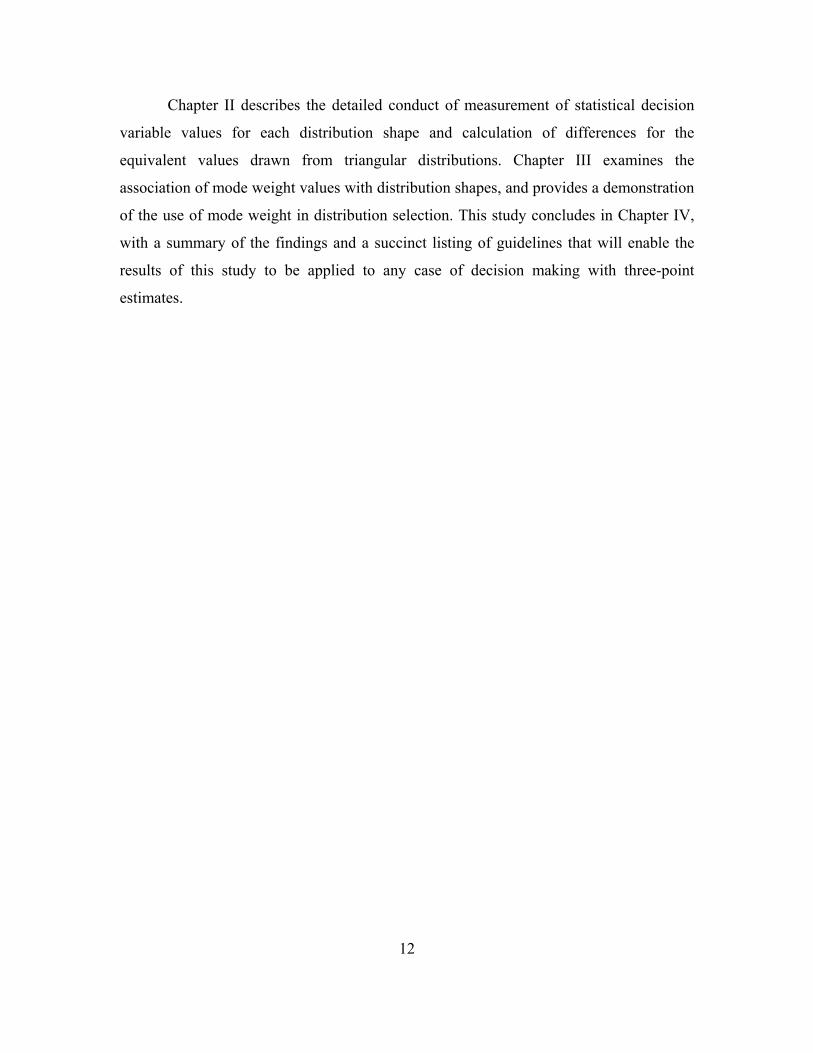
the model itself with these two parameters is normal (0.5,0.167). Figure 6 displays the
probability density functions for the designated boundary uniform and normal-3
distributions for scaled Case A′.
Clearly, for purposes of this study to compare possible alternative distribution
choices to the triangular distribution, the triangle must be included as a choice, with the
scaled model PDF shown previously in Figure 4. A pattern of greater or lesser degree of
peakedness emerges as a discriminator among these three candidate distributions, and
other models ranging in this dimension can be selected from the palette in Figure 3. To
choose an intermediate distribution between the shapes of the triangular and normal
distributions requires something with more weight around the peak than the triangle has
and longer thinner tails out to the end points of the range, but not as peaked nor as narrow
as the normal. A very obvious choice presents itself: the PERT distribution, a special case
of the beta distribution shown in Figure 3. This model was in fact built around the
premise of giving greater weight than the triangle does to the most likely value and is a
staple for project management professionals (PMI 2008). As a bonus the PERT
distribution has the added benefit of utilizing the same modeling parameters as the
triangle, so there is no need for additional transformation to use the provided three-point
values. For Case A′, the scaled data is modeled as PERT (0,0.5,1.0).
22
Figure 6. Boundary Distribution Choices for Scaled Case A′.
The final representative distribution type fits in the shape gap between the
triangular distribution and the uniform distribution. This should be a somewhat broad
distribution and should not have thin tails, but the end points of the range should still
have somewhat lower probabilities than the center. The peak should be flatter and much
less pronounced than the triangle, but certainly visible when compared to the uniform.
That is, it should carry at least a little weight of higher probability at the given mode, but
not a great deal more likelihood than the values near it. A concave ogive-shaped
probability density function fits the intentions nicely, and that is most often modeled by
variations of the beta distribution (GAO 2007) with which most professional cost
estimators will be quite familiar. A four parameter version of the beta model, sometimes
called a beta-general distribution, uses the two typical and shape parameters along
with minimum and maximum parameters to shift and scale the PDF (Vose 2008). This
model can directly use the given three-point estimate minimum and maximum values,
and a small amount of trial-and-error allows one to determine the shape parameters that

23
produce a distribution model that represents the desired shape profile: = = 1.25. This
ogive-shaped distribution is labeled beta-o for ease of discussion. Modeled for this study
for Case A′, it is beta-general (1.25,1.25,0,1.0). Figure 7 displays all five representative
distribution model PDFs for the scaled Case A′ estimate values.
Figure 7. Representative Distribution Model PDFs for Scaled Three-Point Estimate Case A′ = [0,0.5,1.0].
The distribution selections for Case B used to represent the same array of
potential degrees of peakedness require some adjustments from the five model selections
that were used in Case A, due to the asymmetry of the Case B three-point estimate. The
uniform, triangle and PERT distributions can still be used because they utilize the values
of the three-point estimate directly for their distribution parameters. The normal-3
distribution that was previously used in Case A as the best case boundary distribution,
however, is not well suited to represent largely skewed estimates due to its inherent
symmetry. Two choices present themselves to handle this situation: one, to truncate the

24
long side of the skewed estimate by treating the short side as the three-sigma range, and
continue with a normal distribution using that resultant short side computed standard
deviation in conjunction with a mean equal to the three-point mode. Such an assumption
would be fitting if the long side extreme point, either the minimum or the maximum
depending on the {a,b,c} values provided, were actually a singular outlier value that was
atypical of the expected estimate range. That presupposes a high state of knowledge
about the estimate itself and a unique adjustment for a special case, but that runs counter
to the premise of this study where any distribution shape must generically fit the given
three-point estimate. The second choice, which does not truncate the provided estimate
data, is to substitute in place of the normal-3 another distribution that has similar
statistical characteristics but can follow the asymmetrical shape of the skewed estimate
range. A tuned case of the beta distribution can exactly mimic the mean and standard
deviation statistics of the normal-3 distribution for symmetrical cases when = = 4.0,
and can maintain a similar curvature shape and scale of dispersion while fitting it to
skewed three-point estimates by the simple expedient of constraining the sum of its shape
parameters. One can simply use trial and error to adjust the shape parameters, constrained
such that + = 8.0, along with the given minimum and maximum to fit any given
three-point estimate {a,b,c} values regardless of their asymmetry. That is, one “turns the
knob” on just one shape parameter until the resulting skewed beta distribution matches
the three-point estimate proportions. Alternatively, one can use a method described in
Chapter III of this study that uses derived equations to quickly compute and from any
given three-point values (see Chapter III, Section D). By either method, the specific
model that fits the scaled Case B′ is beta-general (3,5,0,1). Figure 8 displays the normal-
like constrained beta PDF, labeled as the beta-n distribution, at increasing degrees of
asymmetry exhibited by the study cases.

25
Figure 8. Examples of Constrained Beta-n Distribution at Various Degrees of Asymmetry.
With the normal-3 substitution for the skewed Case B estimate settled by use of
beta-n in its place, the other representative distribution to adjust is the ogive-shaped beta-
o. Using the same convention of simply constraining the sum of its shape parameters as
was done for beta-n, the beta-o distribution shape and scale can be automatically
maintained throughout varying degrees of asymmetry defined by + = 2.5, as initially
set in Case A. Figure 9 displays scaled beta-o distributions for increasingly skewed
estimates, including the specific Case B′ that is modeled as beta-general (1.17,1.33,0,1).

26
Figure 9. Examples of Constrained Beta-o Distribution at Various Degrees of Asymmetry.
As a result of completing these distribution model adjustments, similar to Case A
there are five representative distributions to examine for Case B: uniform, beta-o,
triangle, PERT and beta-n. The scaled representations of these are modeled as uniform
(0,1), beta-general (1.17,1.33,0,1), triangle (0,0.33,1), PERT (0,0.33,1) and beta-general
(3,5,0,1). These five model PDFs are plotted in Figure 10.

27
Figure 10. Representative Distribution Model PDFs for Scaled Three-Point Estimate Case B′ = [0,0.33,1.0].
Collecting the statistical values of representative distributions for Case C is a
simple matter of continuing the constraining of sums method to select shape parameters
that fit the beta-o and beta-n distributions to the provided Case C three-point estimate
values. The five models that fit the scaled C′ proportions are uniform (0,1), beta-general
(1.06,1.44,0,1), triangle (0,0.125,1), PERT (0,0.125,1) and beta-general (1.75,6.25,0,1).
Figure 11 indicates the PDFs.

28
Figure 11. Representative Distribution Model PDFs for Scaled Three-Point Estimate Case C′ = [0,0.125,1.0].
The final case for this study, the logically extreme limit of asymmetry given in
Case D is modeled using the same distribution types as the previous cases, with shape
parameters computed by the same constrained sum technique. D′ is examined by the PDF
models uniform (0,1), beta-general (1,1.5,0,1), triangle (0,0,1), PERT (0,0,1) and beta
(1,7,0,1). Graphical plots of the D′ models are found in Figure 12.

29
Figure 12. Representative Distribution Model PDFs for Scaled Three-Point Estimate Case D′ = [0,0,1.0].
Each of the four estimate cases have been modeled by potential distribution
choices spanning a realistic range of possible degrees of maturity about the given
estimate, with five distinct distributions for each estimate case. Two statistical measures
from each modeled distribution have been calculated, and combined to represent three
decision variable quantities that could support decision making. Comparison of the
magnitude of differences in the resulting decision variables is the focus of the next
section.
D. ANALYSIS OF DECISION VARIABLE VALUES
1. By Estimate Case
As discussed in Section A of this chapter, the decision variable quantities to be
examined are ′, (′ + ′), and CV′. Since the selection of the decision variables for this
study are combinations of basic statistical measures, one can calculate the values using

30
standard equations for each distribution type (see equation listing in Appendix).
Additionally, any software tool used to model or simulate these types of distribution
models will produce the mean and standard deviation values as a matter of course. For
Case A′, these values for each representative distribution are listed in Table 1, along with
simple percent differences from the equivalent value of the Case A′ triangular distribution
statistics. For graphical reference, the PDF models associated with the statistical values of
each A′ distribution are plotted in Figure 7 in previous Section C.
Table 1. Case A′ Statistical and Comparison Data.
Distribution ′
Difference from
triangular ′ ′ ( ′ + ′)
Difference from
triangular ( ′ + ′) CV′
Difference from
triangular CV′
Uniform (A′) 0.50 0% 0.29 0.79 12% 57.7 41%
Beta-o (A′) 0.50 0% 0.27 0.77 9% 53.5 31%
Triangular (A′) 0.50 0% 0.20 0.70 0% 40.8 0%
PERT (A′) 0.50 0% 0.19 0.69 -2% 37.8 -7%
Normal-3 (A′) 0.50 0% 0.17 0.67 -5% 33.3 -18%
The most obvious comparison one can draw is that the mean values ′ for all
distribution models for this case are identical, and equal to the given mode b′ = 0.5. In
fact, this holds true for all symmetrical distributions one might choose to model the
symmetrical estimate data for Case A, or indeed any symmetrical three-point estimate.
This illustrates a valuable finding: if a decision maker is using the mean, only the mean
and no other statistical value, as the quantity to support his decision then selection of a
distribution to model a symmetrical three-point estimate is arbitrary or even unnecessary
since the mean is equivalent to the provided mode.
If the decision maker was seeking a high-confidence value instead, the (′ + ′)
values for this symmetrical estimate indicate measurable differences between the
triangular distribution and each of the other four choices, with a rather sizeable worst

31
case difference for a uniform. To put this back into the context of the primary research
question, what if one needed the high-confidence value of a given three-point estimate
that was modeled as a triangle by default, but the estimate was actually so rough that a
uniform distribution was more appropriate to the state of knowledge about the estimate?
Could the true high-confidence value actually be different from what would be used in
the triangle-modeled decision, and the decision maker therefore be unknowingly under-
accounting the value of the high-confidence point? Recall that the original three-point
estimate data was transformed into scaled unit space for comparison; the indicated
difference is therefore a percentage of the range magnitude of the three-point estimate
rather than a percentage of the high-confidence value itself. Thus, the high-confidence
value for the decision could be higher by up to 12% of r, not 12% more of x. A widely
spread estimate with large minimum to maximum range magnitude will produce a much
larger error in units of the base value than will a small range magnitude, although they
both represent a change in base value units that is sized as an equal percentage of r.
Uncertain spans of hundreds of units width can introduce error for this decision
scenario in the tens of units, while single digit range magnitudes only generate error sizes
of fractions of a unit. For Case A specifically, the scaled high-confidence point for the
uniform distribution transforms via the scaling equation in Section A back to 31.7 days,
while the high-confidence point for the default triangle transforms to 31.2 days. The half-
day difference in high-confidence duration is only 1.6% longer in actual units of time for
the estimate if it were being modeling as a uniform distribution instead of as a triangle,
due to the small range magnitude and respectively high minimum of three-point estimate
A where r = 6 and a = 27. This error, the worst possible error in this scenario if one were
incorrectly assuming a triangle but should have actually used uniform, is probably not
significant enough on its own to influence or alter the outcome of any decisions about the
given estimated task duration. Yet, consider that this task may run on a schedule critical
path in series with hundreds of other tasks with similar duration estimate uncertainties,
and those unrecognized half-days could quickly add up to a noticeable delay.
Additionally, consider if instead of a short task duration, another estimate for a
symmetrical case had much larger units, for example A2 = {$200k, $500k, $800k}. The

32
scaled models are exactly the same, A2′ = A′ = [0.0.5,1], and A2′ would still have the
uniform-versus-triangle worst case high-confidence error of 12% of r, but this time the
base unit high-confidence values are 673.2 and 622.5 respectively, for an error in $k of
8.1%. As on overrun of a project budget, that would certainly be a noticeable amount,
and could certainly change decisions like budget allocations or even cost-benefit analysis
of alternatives.
Since the true size in base units of the difference of high-confidence values of a
pair of distributions varies with the values of the range magnitude r and minimum a, it
cannot be stated definitively that the high-confidence difference will be significant in all
instances of every symmetrical three-point estimate, even at the largest possible
difference between triangle and uniform. If all possible range magnitude sizes and
minimums are considered for every symmetrical three-point estimate (e.g., A3, A4 ...
AN) with ever-increasing proportions of r / a, then the true difference in base units for
estimate AN approaches the A′ scaled high-confidence difference listed in Table 1. The
curves of differences as a function of range magnitude proportion are plotted in Figure
13, where it can be seen that beyond range magnitude proportions of about 10-to-1 the
differences converge quite closely to the values of the scaled distribution A′ differences
listed in Table 1. True base unit differences are still reasonably close to the scaled
differences at range magnitude proportions down to about 5-to-1, a good analysis
threshold point.

33
Figure 13. Case A High-Confidence Point Base Unit Difference from Triangular as a Function of Range Magnitude Proportion.
Simply converting the horizontal units of Figure 13 to a logarithmic scale allows
observation of another good general threshold point in Figure 14, namely that all high-
confidence point differences become diminishingly small for any distribution choices
when the range magnitude proportion is about 0.2 or less (i.e., when the maximum of the
given three-point estimate is only 20% higher than the minimum). This is a noteworthy
threshold, where differences from triangle for any alternate distribution are small enough
to be negligible and use of a triangular distribution to represent the three-point estimate is
sufficient.
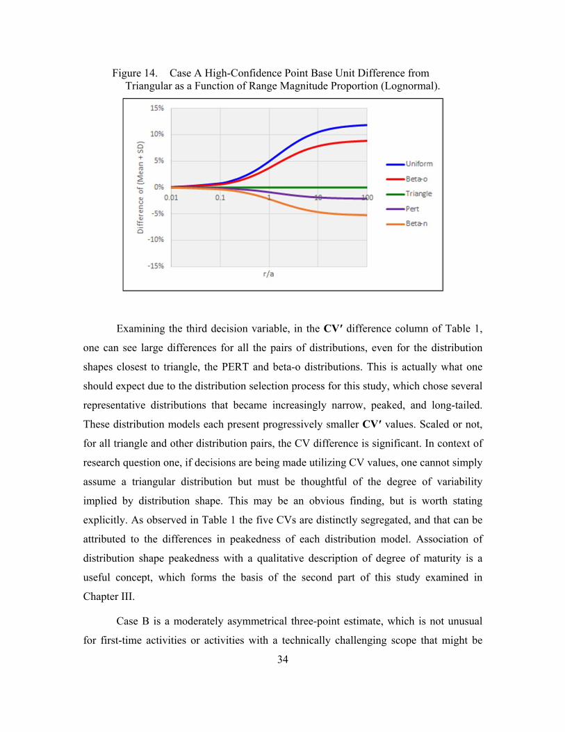
34
Figure 14. Case A High-Confidence Point Base Unit Difference from Triangular as a Function of Range Magnitude Proportion (Lognormal).
Examining the third decision variable, in the CV′ difference column of Table 1,
one can see large differences for all the pairs of distributions, even for the distribution
shapes closest to triangle, the PERT and beta-o distributions. This is actually what one
should expect due to the distribution selection process for this study, which chose several
representative distributions that became increasingly narrow, peaked, and long-tailed.
These distribution models each present progressively smaller CV′ values. Scaled or not,
for all triangle and other distribution pairs, the CV difference is significant. In context of
research question one, if decisions are being made utilizing CV values, one cannot simply
assume a triangular distribution but must be thoughtful of the degree of variability
implied by distribution shape. This may be an obvious finding, but is worth stating
explicitly. As observed in Table 1 the five CVs are distinctly segregated, and that can be
attributed to the differences in peakedness of each distribution model. Association of
distribution shape peakedness with a qualitative description of degree of maturity is a
useful concept, which forms the basis of the second part of this study examined in
Chapter III.
Case B is a moderately asymmetrical three-point estimate, which is not unusual
for first-time activities or activities with a technically challenging scope that might be

35
considered somewhat risky and have a presumption of unexpected but possible high end
values somewhat larger than the low end nominally expected values (NASA 2007). All of
the representative distributions fit to this case are right-skewed, except of course for the
uniform that is always symmetrical between its minimum and maximum. This skewness
results in a mean for each distribution that is higher than the mode of the given three-
point estimate. Table 2 lists the respective statistics and decision variable values for the
scaled B′ versions of the five representative distribution shapes, which were depicted
graphically in Figure 10 in Section C.
Table 2. Case B′ Statistical and Comparison Data.
Distribution ′
Difference from
triangular ′ ′ ( ′ + ′)
Difference from
triangular ( ′ + ′) CV′
Difference from
triangular CV′
Uniform (B′) 0.50 13% 0.29 0.79 21% 57.7 23%
Beta-o (B′) 0.47 5% 0.27 0.73 12% 57.2 22%
Triangular (B′) 0.44 0% 0.21 0.65 0% 46.8 0%
PERT (B′) 0.39 -13% 0.18 0.57 -12% 47.4 1%
Beta-n (B′) 0.37 -16% 0.16 0.54 -18% 43.0 -8%
For the selected boundary distribution shapes normal-like beta-n and uniform,
scaled absolute differences of means from the triangle can be as high as 16% and 13%
respectively. The smallest difference in scaled mean values occurs between the ogive-
shaped beta-o distribution and the triangle, with the scaled beta-o mean being 5% higher
than the scaled triangle mean. Even this smallest size of a difference would certainly trip
most cost variance reporting thresholds, but again the differences in Table 2 are for
scaled distributions and are percentages of r, not x. Plots similar to Figures 13 and 14
reinforce the applicability of the 5-to-1 and 20% range magnitude proportion thresholds
for utilizing the scaled differences to assess three-point estimates at this moderate degree
of asymmetry. There is no question that variations of 5% or more could easily alter the

36
outcomes of decisions based only on the mean value of a triangularly modeled three-
point estimate if the alternate distribution was known and modeled instead. The
differences from triangular are larger still for the high-confidence point, where values
drawn would be further rightward down the long tail of each distribution. The beta-o still
exhibits the smallest scaled difference, a clearly significant 12%, and all other
distributions have increasingly larger differences up to the uniform distribution, which
produces a substantial 21% difference from the triangular high-confidence point. For CV′
values, as with Case A, they are distinctly sequenced for each distribution, although the
PERT and triangle CVs approach each other when skewed this much. While the
asymmetry of Case B alters the relative differences somewhat compared to the same Case
A pairs and they are slightly smaller overall, the general spread and order holds. All three
decision variable observations substantiate a general finding for all moderately skewed
estimates: whether decisions are based upon means, high-confidence points, or
coefficients of variation, distribution shape choice will measurably affect the statistical
values used to support those decisions, and uninformed usage of triangular distribution
models by default will introduce sizeable error.
The third case examined in this study is the highly asymmetrical three-point
estimate provided in Case C. Here the maximum is many times further away from the
mode than the minimum is, such that the vast majority of the minimum to maximum
range is above the mode. No matter the choice of distribution model type, except for the
uniform again, the proportions of the given three-point values will result in an extremely
right-skewed distribution with a very long tail extending out to the maximum, as depicted
in the PDF graphs in the previous section in Figure 11. With this severely asymmetrical
condition, the largest scaled difference of the mean is for the normal-like beta-n
distribution, a staggering 42% lower than the triangular mean. Even with the base units
for range magnitude and minimum of this example case in the single digits of pounds,
when transformed this is still a significantly different mean value that could affect
engineering trades. In scaled terms, even the smallest difference one could expect if an
ogive-shaped beta-o were instead the appropriate model is still 13% higher than the mean

37
of the respective scaled triangular distribution. All the Case C′ statistical values for the
common decision variables are listed in Table 3.
Table 3. Case C′ Statistical and Comparison Data.
Distribution ′
Difference from
triangular ′ ′ ( ′ + ′)
Difference from
triangular (′ + ′) CV′
Difference from
triangular CV′
Uniform (C′) 0.50 33% 0.29 0.79 32% 57.7 -3%
Beta-o (C′) 0.43 13% 0.26 0.69 15% 62.2 5%
Triangular (C′) 0.38 0% 0.22 0.60 0% 59.3 0%
PERT (C′) 0.25 -33% 0.16 0.41 -31% 65.5 10%
Beta-n (C′) 0.22 -42% 0.14 0.36 -40% 63.0 6%
The size of the differences for Case C′ high-confidence points are exaggerated
even further than they were in the moderately skewed Case B′. From the smallest
absolute difference from triangle of 15% for beta-o, to largest difference of 40% for beta-
n, all are significant and could dramatically change decision outcomes. Oddly, the CV′
differences shrink in size for Case C when compared to Case B. This phenomenon is a
result of the extreme asymmetry of these distributions, as all of the tailed distribution
CVs have grown to now exceed that of the uniform, which had originally been the most
uncertain distribution type with the largest CV′ value in the preceding Cases A and B.
This effect coupled with the preceding observations for mean and high-confidence point
differences leads to the general finding from examination of all Case C decision
variables: when three-point estimates exhibit extreme asymmetry, all distribution models
for them have higher than typical coefficients of variation, and statistical measures are
very sensitive to distribution shape choices. Care should be taken to explicitly model any
such estimate, with consideration given to decomposing and extracting off-nominal
outliers from the nominal estimate range for individual decision handling of the outlier.

38
Case D takes the effects of asymmetry to the extreme logical limits. Here, the
various distribution PDFs in Figure 12 are barely recognizable, no longer peaked with
tails extending off in both directions. Now they appear almost as asymptotes approaching
the limit of one maximum likelihood end-point at varying closure rates. Yet, each
distribution still retains a semblance of its originally intended role in the spread of
degrees of uncertainty. The uniform distribution is exactly the same as it has been for all
cases, flat constant probability for all values. Beta-o is still concave throughout the range,
although it is now a single fat rounded tail leveling off toward flatness as it approaches
the significant end-point. The triangular distribution plots a linear diagonal with its right-
triangle slope defined by the range magnitude. PERT is a fully convex curve, all long thin
tail falling away from the prominent peak now situated at the extreme end-point. What
was originally the normal-like beta-n is even more deeply convex than PERT, displaying
a veritable exponential-like spike at the most likely end. The comparative PDF plot of all
these distributions was displayed previously in Figure 12, and the accompanying scaled
Case D′ statistical values are found in Table 4.
Table 4. Case D′ Statistical and Comparison Data.
Distribution ′
Difference from
triangular ′ ′ ( ′ + ′)
Difference from
triangular ( ′ + ′) CV′
Difference from
triangular CV′
Uniform (D′) 0.50 50% 0.29 0.79 39% 57.7 -18%
Beta-o (D′) 0.40 20% 0.26 0.66 16% 65.5 -7%
Triangular (D′) 0.33 0% 0.24 0.57 0% 70.7 0%
PERT (D′) 0.17 -50% 0.14 0.31 -46% 84.5 20%
Beta-n (D′) 0.13 -63% 0.11 0.24 -59% 88.2 25%
Starting from the narrowest distribution, beta-n, the mean for each distribution
moves steadily further away from the significant end point (i.e., the minimum in this
case) for each distribution shape normally representing a step increase of the degree of

39
uncertainty. When compared to the triangular distribution in the middle of the pack, the
beta-n delivers the largest difference in scaled mean, the most extreme error possible for
any decision scenario at 63% less than the triangular mean for the same three-point
estimate. On the other end of the distribution shape spectrum, the uniform’s difference is
comparably large at fully 50% higher than triangle. Here the triangle’s closest neighbor
with the smallest difference of means is again the beta-o, and it is still 20% higher in this
most extremely skewed condition. High-confidence points have comparably large
variances, with absolute value differences ranging from 16% to 59%. CV behavior is
even more abnormal than with Case C, exhibiting conceptually reversed observations
from standard experience with the uniform now lowest and each progressively more
peaked distribution bizarrely presenting an increasingly larger CV. One would not expect
to utilize CV for decision making in this type of extreme case. A general finding for this
case related to decision variable differences is the same as for Case C only more so:
maximum size of statistically-based decision variable variation due to distribution choice
occurs at the extreme limit of asymmetry.
2. By Decision Variable
Since analysis of each of the separate three-point cases indicates such a significant
effect due to asymmetry, a perhaps more useful set of observations can be made when
examining each decision variable for each distribution type across all Cases A-D and the
points between, to the full extent of asymmetrical orientations possible. Figure 15 shows
the mean for each scaled distribution type as a function of its relative asymmetry, and
Figure 16 computes the size difference from triangle for scaled means of each type of
distribution throughout the entire range of possible asymmetry.

40
Figure 15. Scaled Distribution Mean Shift as a Function of Asymmetry.
Figure 16. Scaled Distribution Mean Difference from Triangular Mean as a Function of Asymmetry.
Here the axes are quite different than the previous PDF graphs; the horizontal axis
indicates the relative position of the mode b′ within the distribution range, which is the

41
distribution peak position as a percentage of the range magnitude and serves as a form of
shorthand for the degree of asymmetry. The left edge, zero on the horizontal axis, is the
limit of every right-skewed distribution with the mode equal to the minimum; 0.5 in the
center is any symmetrical distribution with the mode equidistant from its end points; and
the far right of the graph at 1.0 is the extreme limit of left-skewed distributions where the
mode is equal to the maximum. The vertical axis is either the corresponding scaled mean
value as in Figure 15, or the percent difference of that distribution’s mean from a same-
skewed triangle mean. Note that the four specific estimate cases in this study would be
represented by vertical lines drawn at D′ = 0, C′ = 0.125, B′ = 0.33 and A′ = 0.5. It is
clear from Figure 16 that for every distribution choice the absolute size of the difference
from triangle mean is heavily influenced by the asymmetry of the estimate being
modeled. When making decisions based on mean values from any given three-point
estimate, if the estimate basis is either very rough or very mature then a triangular
distribution should not be used, unless the estimate is symmetrical. If the estimate
maturity is somewhere between those two subjective extremes (i.e., excluding uniform or
beta-n) then a triangular distribution can be a good approximate model through small
amounts of skewing. When the asymmetry of a given three-point estimate is more severe
than 2-to-1 (i.e., scaled mode less than 0.33 or more than 0.66) explicit distribution
selection is necessary.
Graphing the high-confidence points through the full range of asymmetry is a
similar exercise. Figure 17 plots the scaled SD for each distribution as a function of
asymmetry, and when combined with the mean values from Figure 15 produces the
generic high-confidence point value (i.e., [′ + ′]) across the asymmetry range as shown
in Figure 18. When these values for each distribution type are compared to the high-
confidence point value of the triangular distribution, the difference is plotted in Figure
19.

42
Figure 17. Scaled Distribution SD Shift as a Function of Asymmetry.
Figure 18. Scaled Distribution High-Confidence Point Shift as a Function of Asymmetry.

43
Figure 19. Scaled Distribution High-Confidence Point Difference From Triangular as a Function of Asymmetry.
When high-confidence values from a three-point estimate are the basis of decision
making, explicit choice of distribution shape should be used for all symmetrical and
right-skewed cases. For less common left-skewed cases, a triangle approximation has
reasonably small error near the 2-to-1 asymmetry point (i.e., 0.66) and possibly tolerable
error for greater left-skewed estimates if the range magnitude is also small.
Coefficient of variation is easily determined from values in Figures 15 and 17,
and the resulting scaled CV as a function of asymmetry is plotted in Figure 20.

44
Figure 20. Scaled Distribution Coefficient of Variation Shift as a Function of Asymmetry.
The typically expected stratification of CV for each distribution is seen for all
symmetrical and left-skewed distributions, and also holds for slightly right-skewed
distributions. As experienced when examining Cases C and D, any right-skewed
asymmetry much beyond the 2-to-1 point (i.e., scaled mode smaller than 0.33) begins to
display abnormal CV behavior. This is an artifact of a rapidly shrinking denominator (
with a generally steady numerator (). When CV differences from triangle are computed
for each distribution type, the unusual set of curves in Figure 21 appear.
45
Figure 21. Scaled Distribution Coefficient of Variation Difference from Triangular as a Function of Asymmetry.
CV differences can be large in almost all cases of asymmetry, and the CV values
themselves behave unusually in the extremely right-skewed region where the difference
is relatively small. Since CV is innately sensitive to the selected shape of a distribution, if
it is being used as the primary basis for a decision, the triangular distribution model
should never be automatically assumed, only used by explicit choice.
When conducting program analyses and basing decisions on three-point estimates,
triangular distributions are commonly utilized to model the estimate and produce
statistical measures. This study contends that default usage of triangular distribution
models can introduce measurable error in the decision making statistical values if a more
appropriate distribution type is better suited to the state of knowledge about the given
estimate but not used. By modeling a representative suite of distribution shapes to signify
boundary-to-boundary states of knowledge for specified cases of three-point estimates,
and by extrapolation through the full range of asymmetry possible by any three-point
estimate, this study has quantitatively measured the size of error a decision maker might
unknowingly accept from use of triangular distribution model by assumption rather than
explicit selection. This is not to suggest that the triangle model is not useable or useful; it

46
is very well suited for modeling some of the most frequently encountered types of three-
point estimates, such as symmetrical or only slightly skewed estimates with relatively
small range magnitudes and medium basis of maturity. Outside of these situations, other
distribution choices are warranted to avoid introducing error by model shape. Simplified
guidelines from findings in this chapter’s analysis appear in tabular form in the
conclusions in Chapter IV.
When explicitly choosing distribution types to accurately model given estimates,
several concepts from this chapter come into consideration to help guide the selection
process. Chapter III of this study examines and simplifies them, and recommends an
intuitive method for easy selection of a distribution model for any three-point estimate.

47
III. SELECTION OF ALTERNATIVE DISTRIBUTION TYPES
A. QUALITATIVE RELATIONSHIPS OF DISTRIBUTIONS
In Chapter II, several observations showed that there are circumstances in
modeling three-point estimates when explicit selection of an alternative distribution is
called for. As displayed in Figure 3 in Chapter I, there are many potential choices of
distribution models, but few with the attractive simplicity of the most commonly used
model: the triangular distribution. Several concepts were touched upon in the Chapter II
that can be leveraged to produce a simplified set of guidelines to assist in the complex
distribution selection process: 1) distribution peakedness can be associated with the
maturity of the basis of an estimate or state of knowledge about the value being
estimated; 2) stratification of coefficients of variation occurs with distribution shapes that
have greater or lesser amounts of dispersion away from their modes, and quantitatively
relates distribution statistical values to their peakedness; and 3) differing levels of
constrained sums of shape parameters for beta distributions provide for distinctly
differently peaked shapes that retain their relative scale of dispersion throughout the full
range of possible asymmetry. Taken together, these concepts allow for a cohesive
quantitative scale consistently proportional to qualitative degree of confidence in the
basis of any given three-point estimate, simply called mode weight and labeled d.
B. VISUAL SURVEY
Consider a visual survey of the PDFs of the representative distributions used in
the study in Chapter II such as Figure 7, repeated here as Figure 22 for reference.

48
Figure 22. Representative Distribution Model PDFs for Scaled Three-Point Estimate Case A′ = [0,0.5,1.0].
The normal distribution, or normal-3 or beta-n, presents the familiar bell-shaped
curve with relatively pointed peak, steep sides enclosing a narrow body, tapering down to
rapidly thinner and thinner tails that extend far from the body to the distant end points.
The very highest probabilities are clustered relatively tightly at values close to the mode
while only a short distance away the probabilities are much lower, and odds become
vanishingly remote out near the end points that can be generally be viewed as outlier
values of the estimated quantity. Progressing in order of typical step increases of CV,
indicating larger dispersions, one sees the PERT distribution. While it is shaped similarly
to the normal, the differences of its curvature describe much about the shift of
probabilities in this model. Its peak is blunted, with a wider more loosely clustered body
providing greater chances of occurrence to values further from the mode. The slopes are
less steep making the middle-range values not vastly less likely than the mode, and the
tails cover a much shorter range of values to the end points and are much thicker, lending

49
some reasonable possibility of occurrence to the values further out toward the ends. The
triangular distribution is in the middle of the pack of increasing dispersions, thickening
the tails and broadening the shoulders of the body until a fixed linearly decreasing rate of
lower probabilities spreads steadily and shallowly down from the mode to finitely
possible minimum and maximum values. Next, the ogive-shaped beta-o has no tails to
speak of, the clustering of its body values so diffuse that it is simply a wide flat-topped
hump. The mode is still visible, but with a corresponding probability not much greater
than the vast majority of its neighbors. Finally, the uniform distribution has no visibly
distinguishable mode, and its end-points are the complete conceptual opposite of outliers,
being just as credible and just as likely as the provided mode value and every other value
in the range with the same flat probability. This distribution shape progression from
mode-centric, tightly clustered normal, through looser clustering, broadening and
flattening, to the mode-ignorant flat uniform distribution exhibits the steady scaling
influence of an intrinsic factor such as mode weight at work.
C. QUALITATIVE MODE WEIGHT
As described in Section A of the preceding chapter, when the representative
distributions in this progression were selected for study, they were intended to cover the
broad spectrum of uncertainty about a given estimate. Not uncertainty in the sense that
more uncertainty would mean the minimum to maximum range magnitude of the
estimated quantity would be greater; rather uncertainty about the state of knowledge of
the basis supporting the three-point estimate itself. Very mature estimates supported by
vast experience with a large amount of actual observations of highly similar scope could
approach what might be expected from a purely objective statistical study, and might
exhibit as close to normal-like certainty about the most likely value as a subjective
estimate would allow. This state of knowledge would correspond to very high subjective
confidence in the mode value and very high mode weight. When estimate extrapolations
are based upon only a few actual data points or when the similarity of analogous scope is
tenuous, SMEs and analysts become progressively less confident in the superiority of
their provided mode. When the scope is virtually unknown and rough estimates are
merely educated guesses, the confidence that the mode point of a provided three-point

50
estimate is truly the most likely value is very low, and therefore the mode weight is very
low. Ranked classes of estimates like this are recognized by the Association for the
Advancement of Cost Engineering, International and follow a graduated scale of estimate
maturity as one of the segregating criteria (2011). Ordered this way, the qualitative
progression related to estimate maturity follows the same sense of decreasing mode
weight as the visual survey did, and suggests an easy association. A straightforward five-
step Likert scale for assigning an intuitive qualitative value to the basis of estimate
maturity can accompany a provided three-point estimate, and provide a credible rationale
for distribution model selection. This scale is indicated in the first two columns of Table
10 in the conclusion of this study, with matching distribution shape choices indicated to
model the three-point estimates they accompany. For best results, collecting this
“qualitative fourth point” from the SME during elicitation of their quantified three-point
estimate assures that the subjective confidence in elicited mode weight assessment is
appropriate for the estimator’s belief. It is not strictly necessary, however, to alter or re-
execute the existing elicitation methods of a program to gain this beneficial data. If three-
point estimates have already been provided but lack a qualitative fourth point given by
the estimator, analysts and modelers can quickly and consistently assume an equivalent
qualitative level of the estimate maturity based on any additional data they may have on
hand regarding that and other past estimates in the program. Complete lack of any
supplemental information to help guide the assumption of estimate maturity is suggestive
of a Very Low designation, and progressively more supportive information steps up the
estimate maturity score intuitively from there. One of the five representative distribution
shapes used throughout this study is associated with each qualitative level, and can be
easily modeled in any statistical software tool with the three-point estimate quantities
given. Of these, only the beta-o and beta-n distributions require any kind additional
processing of the simple three-point parameters to enable their modeling, and those are
handled via a straightforward substitution equation derivation.
D. QUANTITATIVE MODE WEIGHT
Underlying the qualitative scale of the last section, a quantitative basis can be
developed. The mode weight concept was used explicitly in the creation of the PERT

51
distribution (Vose 2008), where the scheduling PERT network assumption was used that
an average task duration was four times more sensitive to the most likely value of a three-
point estimate than it was to either the optimistic or pessimistic end-point durations. This
weighting scheme constrains the mean of a beta distribution that fixes the shape
parameters relative to the provided three-point values. The parameterization all occurs in
the background with the shape parameters already fully defined in terms of only the
points {a,b,c}, as well as the typical distribution equations for mean and standard
deviation. David Vose (2008) cleverly extends that derivation to a create a modified
PERT distribution, where the fixed PERT network assumption is generalized and
replaced by a variable that can tune the sensitivity of the most likely value, thus fixing the
shape parameters of a default PERT distribution to a constrained set that is comparatively
more or less dispersed, varying with the now quantitative fourth point, d. Thus, a single
“knob” can be turned to completely define and shape parameters for any mode
weight for any three-point estimate, and mimic all the representative distributions used
previously in this study. Most modeling software tools allow use of PERT distributions
directly, but not Vose’s modified PERT with a fourth point parameter for mode weight;
however, nearly all tools support the use of some form of the beta-general distribution.
Since PERT was designed as a special case of a beta distribution, modified PERT with
the mode weight parameter d can also be computed as a beta-general distribution that can
be modeled, as follows:
Given an estimate {a,b,c,d}, where a ≤ b ≤ c, and 0 ≤ d
From PERT equations (Appendix): ( 4* )
6
a b c
Mod-PERT version (Vose 2008): ( * )
( 2)
a d b c
d
, d = 4 for standard PERT.
From beta-general equations (Appendix), solved for each shape parameter:
( )*(2* )
( )*( )
a b a c
b c a

52
*( )
( )
c
a
By substituting from mod-PERT:
( * )*(2* )
( 2)
( * )*( )
( 2)
a d b ca b a c
d
a d b cb c a
d
( * )*
( 2)
( * )( 2)
a d b cc
d
a d b ca
d
The shape parameters are fully defined in terms of {a,b,c,d}, although the
equations do not algebraically simplify well. This complexity can be overcome with
practical spreadsheet formula use, and the outcome can then be modeled as beta-general
(,,a,c). These are the equations used in Chapter II to calculate shape parameters for all
designated special versions of beta with a fixed mode weight value (i.e., beta-o where d =
0.5, and beta-n where d = 6.0). Discovery of the specific d value that produced statistical
values matching those of the desired distribution was a matter of trial-and-error “turning
the knob” and varying the value of d until the resulting beta-general model output the
specific values of the target distribution for the symmetrical estimate case. After that,
calculating the shape parameters for every state of asymmetry for a given fixed-d
distribution type like beta-o led empirically to the discovery that the sum of and was
always constant regardless of how skewed the {a,b,c} points were and established the
constrained sum method described in Chapter II.
These two equations can be mechanized with pre-defined fixed values of d to
quickly produce shape parameters for the beta-o and beta-n distributions for any provided
three-point estimate, and modeled for analysis simply with beta-general. This means all
five discrete representative distributions can be simply selected using the qualitative

53
fourth point per the first two columns of Table 10 in the conclusion, and simply modeled
using the corresponding mode weight detent value in the last column along with the given
three-point estimate values. A savvy analyst might recognize that three of the five
distributions in the representative set are variations of beta, and the uniform distribution
results by default when the two shape parameter equations are run with d = 0, or simply
any beta-general when = = 1. If one considers that the statistical mean and standard
deviation values of a symmetrical triangular distribution can be duplicated by matching
moments of a beta distribution exactly as was done by beta-n for the normal-3, a mode
weight value for this triangle-like dispersion can be set and used as a beta-t distribution
throughout the span of asymmetry. With this substitution, one can model every possible
estimate case with a custom-fit beta-general model using fully quantitative 4-pt.
estimates, ranging the continuous mode weight variable 0 ≤ d ≤ 6 to fine-tune an exact
mode weight at or even between the “detent” values that automatically match shape
parameters to the representative distributions. Such a modeling layout would enable real-
time graphing that could be utilized to augment SME elicitation of three-point estimate
quantities with on-the-fly turning of knob d to auto-generate distributions without even
needing to choose a discrete distribution model shape. It would also greatly simplify
spreadsheet formula construction for highly complex decision models, with only one
model type scripted in and one of the entered parameter values “selecting” the
distribution shape by virtue of its value. Modeling all estimates as beta distributions in
this fashion would also establish excellent conjugate priors for any future endeavors in
Bayesian updating of estimates. All just as simple as {a,b,c,d}.
Revisiting the secondary research question of this study, when distribution
modeling other than triangular is called for, can alternative distributions be simply,
intuitively and credibly selected? Yes, because the qualitative scale described previously
and listed in Table 6 in the conclusion is certainly simple, and the companion mode
weight concept with estimate maturity judgment should be very easy to grasp by any
SME, estimator or modeler.

54
E. PRACTICAL APPLICATION
As an illustration of these findings put into practice, consider a type of decision
that is fairly commonplace in systems engineering execution: balanced down-selection of
a design configuration. In the following example, the decision is a choice between two
discrete options, and is supported quantitatively by routine cost-benefit analysis (CBA) in
the form of simple benefit-to-cost ratios (Boardman 2014) and displays of Pareto
optimality (De Neufville and Scholtes 2011) via plots of cost as an independent variable
(CAIV).
The benefit attribute figures of merit (FOM) for this trade are the mass of the
respective designs, determined by the decision maker to be critically important, and the
time for installation of the components into the system since the assembly activities are
on the critical path of the development program schedule. For both FOMs, the preference
is for the FOM to be as low as possible, and the decision maker requests high-confidence
estimates as the basis for the analysis. The first option, Design 1, is at a pre-PDR state of
maturity and estimates for its mass, installation duration, and cost are the result of expert
elicitation which yielded three-point estimates to capture subjective uncertainty. The
values of these three estimates were seen earlier in this study as estimate Case C (mass),
Case A (duration), and Case B (cost). The second option in this decision, Design 2, is a
modification of well understood heritage hardware. The estimate data for this option is
based principally on actual measurement of previous implementations of this design, but
with some subjective uncertainty elicited to account for the nature of the modifications.
The minimum, most likely, and maximum values of the three-point estimates of all
FOMs for both design options are listed in Table 5. The common practice of modeling
the uncertainty via a triangular probability distribution is utilized for all FOMs, and the
mean and standard deviation are computed from the resulting PDFs and summed to
produce the high-confidence estimates.
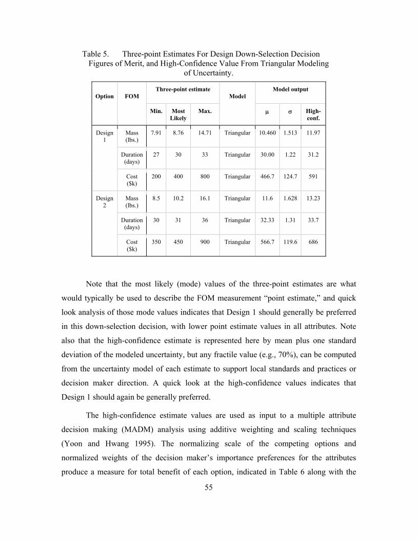
55
Table 5. Three-point Estimates For Design Down-Selection Decision Figures of Merit, and High-Confidence Value From Triangular Modeling
of Uncertainty.
Option
FOM
Three-point estimate Model
Model output
Min. Most Likely
Max. High-conf.
Design 1
Mass (lbs.)
7.91 8.76 14.71 Triangular 10.460 1.513 11.97
Duration (days)
27 30 33 Triangular 30.00 1.22 31.2
Cost ($k)
200 400 800 Triangular 466.7 124.7 591
Design 2
Mass (lbs.)
8.5 10.2 16.1 Triangular 11.6 1.628 13.23
Duration (days)
30 31 36 Triangular 32.33 1.31 33.7
Cost ($k)
350 450 900 Triangular 566.7 119.6 686
Note that the most likely (mode) values of the three-point estimates are what
would typically be used to describe the FOM measurement “point estimate,” and quick
look analysis of those mode values indicates that Design 1 should generally be preferred
in this down-selection decision, with lower point estimate values in all attributes. Note
also that the high-confidence estimate is represented here by mean plus one standard
deviation of the modeled uncertainty, but any fractile value (e.g., 70%), can be computed
from the uncertainty model of each estimate to support local standards and practices or
decision maker direction. A quick look at the high-confidence values indicates that
Design 1 should again be generally preferred.
The high-confidence estimate values are used as input to a multiple attribute
decision making (MADM) analysis using additive weighting and scaling techniques
(Yoon and Hwang 1995). The normalizing scale of the competing options and
normalized weights of the decision maker’s importance preferences for the attributes
produce a measure for total benefit of each option, indicated in Table 6 along with the

56
high-confidence cost estimate of each design project, expressed as net present value
(NPV).
Table 6. Multiple Attribute Decision-Making Analysis for Design Down-Selection Decision Using High-Confidence Value from Triangular
Modeling of Uncertainty.
Attribute Weight Design 1: High-confidence estimate, triangular
Design 2: High-confidence estimate, triangular
Scale Factor
Raw Scaled Weighted Raw Scaled Weighted
MINIMIZE Mass (lbs.)
0.8 11.97 1.000 0.800 13.23 0.905 0.724 11.97
MINIMIZE Duration (days)
0.2 31.2 1.000 0.200 33.7 0.928 0.186 31.2
Total Benefit 1 1.000 0.910
Cost [NPV constant FY11] ($k)
591 686
B/C (scaled-weighted benefit/$k)
1.691 1.325
One can examine the ratio of the total benefit measure to cost in the bottom row
of Table 6, or with a variety of simple graphical interpretations, like the column chart in
Figure 23, to compare the relative magnitudes of this indicator for preference.
When the total benefit measure for an option is plotted in two-dimensional
fashion as an x-y scatter plot with the cost estimate as the independent variable,
additional analytical trade-off comparisons become possible, such as determination of
relative position of various options to a Pareto optimal efficient frontier or cost threshold,
identification of dominated alternatives, and clustering of options suggesting further
compromise design trades that can be explored. The binary condition of this design
down-selection decision makes for a basic yet unambiguous CAIV plot, in Figure 24. By
all quantitative indications in this CBA, selection of Design 1 is supported as the
recommended choice for the decision maker in this case.

57
Figure 23. Benefit-to-Cost (B/C) Ratio of Options for Design Down-Selection Decision Using High-Confidence Value from Triangular Modeling of
Uncertainty.
Figure 24. Cost as an Independent Variable (CAIV) Plot for Design Down-Selection Decision Using High-Confidence Value from Triangular
Modeling of Uncertainty.

58
Now recall the discussion of the elicitation of three-point estimates for the FOM
values of each option. This study has found that elicitation information provides data to
support guidance to select distribution model shapes possibly more appropriate than
triangle for the state of knowledge about the subjective uncertainty. Design 1 is an
immature design not yet through PDR, so engineers do not convey strong confidence in
the mode of its mass estimate remaining very near that value through iterative design and
analysis cycles. The duration estimate is based on judgment only, without supporting data
of actual task completions, and the cost estimate is of rough order of magnitude (ROM)
fidelity at best. Qualitatively, all three are judged to have “Low” estimate maturity and/or
confidence about the mode values. From Table 10 in the conclusion, the recommended
distribution model shape for all three of these FOMs is beta-o, the distribution that is an
ogive-shaped flattened hump that concavely spans the minimum to maximum range
without tails.
In contrast, Design 2 estimates are drawn from an experience base with a heritage
design, with prior actual data to support the provided three-point estimates, strong
confidence in the mode values as being truly the most likely points, and the extreme end
point values being seen as outliers. All three of these FOM estimates are judged as “Very
High” maturity, and a normal distribution would be appropriate. Since the provided three-
point parameters are not symmetrical, beta-n is the recommended model shape. In both
design option cases, the qualitative guidance that allows designation of a distribution
shape also provides a quantitative detent value for the mode weight parameter d, which is
then used in the derived customized beta distribution equations from the previous section
to compute the beta distribution shape parameters for each three-point estimate. The
additional model parameters and shape designation labels are included with the original
three-point values for all FOMs in Table 7.

59
Table 7. Three-Point Estimates for Design Down-Selection Decision Figures of Merit, and High-Confidence Value from Beta Distribution
Modeling of Uncertainty.
Option
FOM
Three-point estimate Est.
maturity, mode conf.
Model
Model parameters Model output
Min. Most Likely
Max. d High-conf.
Design 1
Mass (lbs.)
7.91 8.76 14.71 L Beta-o 0.5 1.063 1.438 10.800 1.797 12.60
Duration (days)
27 30 33 L Beta-o 0.5 1.250 1.250 30.00 1.60 31.6
Cost ($k)
200 400 800 L Beta-o 0.5 1.167 1.333 480.0 160.0 640
Design 2
Mass (lbs.)
8.5 10.2 16.1 VH Beta-n 6 2.342 5.658 10.725 1.153 11.88
Duration (days)
30 31 36 VH Beta-n 6 2.000 6.000 31.50 0.87 32.4
Cost ($k)
350 450 900 VH Beta-n 6 2.091 5.909 493.8 80.6 574
As with the previous analysis using triangular modeling, the mean and standard
deviation are computed for each uncertainty distribution from the same original three-
point estimate parameters, modeled this time as beta-o and beta-n respectively, and
summed to produce the high-confidence estimate value for each FOM. The CBA
methods are repeated using the new high-confidence point values as input, with results
shown in Table 8 and Figures 25 and 26.
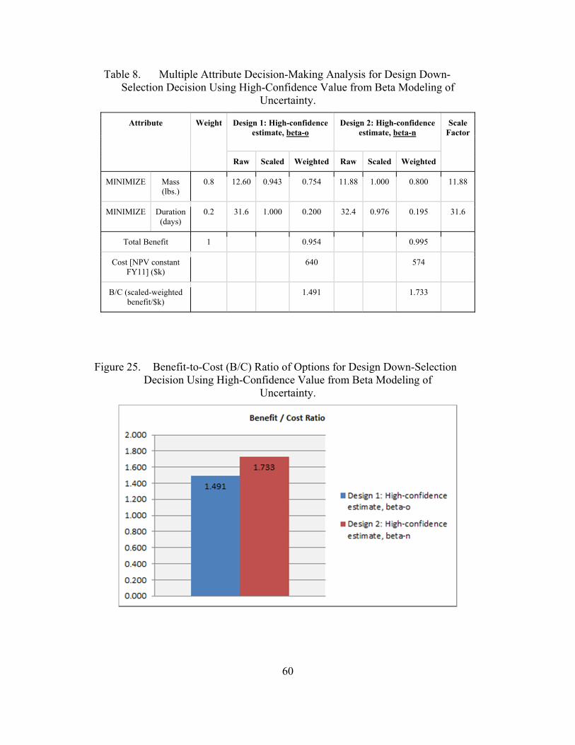
60
Table 8. Multiple Attribute Decision-Making Analysis for Design Down-Selection Decision Using High-Confidence Value from Beta Modeling of
Uncertainty.
Attribute Weight Design 1: High-confidence estimate, beta-o
Design 2: High-confidence estimate, beta-n
Scale Factor
Raw Scaled Weighted Raw Scaled Weighted
MINIMIZE Mass (lbs.)
0.8 12.60 0.943 0.754 11.88 1.000 0.800 11.88
MINIMIZE Duration (days)
0.2 31.6 1.000 0.200 32.4 0.976 0.195 31.6
Total Benefit 1 0.954 0.995
Cost [NPV constant FY11] ($k)
640 574
B/C (scaled-weighted benefit/$k)
1.491 1.733
Figure 25. Benefit-to-Cost (B/C) Ratio of Options for Design Down-Selection Decision Using High-Confidence Value from Beta Modeling of
Uncertainty.
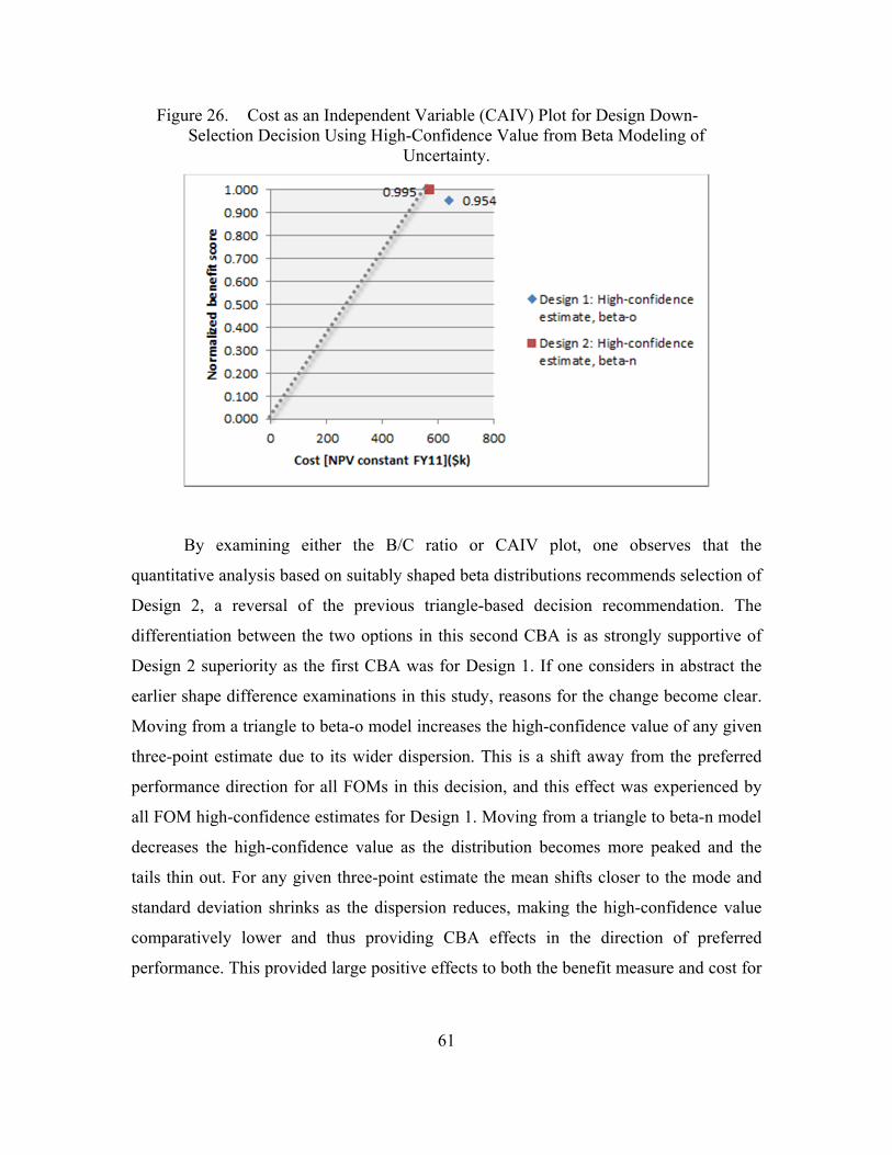
61
Figure 26. Cost as an Independent Variable (CAIV) Plot for Design Down-Selection Decision Using High-Confidence Value from Beta Modeling of
Uncertainty.
By examining either the B/C ratio or CAIV plot, one observes that the
quantitative analysis based on suitably shaped beta distributions recommends selection of
Design 2, a reversal of the previous triangle-based decision recommendation. The
differentiation between the two options in this second CBA is as strongly supportive of
Design 2 superiority as the first CBA was for Design 1. If one considers in abstract the
earlier shape difference examinations in this study, reasons for the change become clear.
Moving from a triangle to beta-o model increases the high-confidence value of any given
three-point estimate due to its wider dispersion. This is a shift away from the preferred
performance direction for all FOMs in this decision, and this effect was experienced by
all FOM high-confidence estimates for Design 1. Moving from a triangle to beta-n model
decreases the high-confidence value as the distribution becomes more peaked and the
tails thin out. For any given three-point estimate the mean shifts closer to the mode and
standard deviation shrinks as the dispersion reduces, making the high-confidence value
comparatively lower and thus providing CBA effects in the direction of preferred
performance. This provided large positive effects to both the benefit measure and cost for

62
Design 2, and coupled with the negative effects suffered by Design 1 to overturn the
recommendation of the first CBA.
This example demonstrates the utility of all aspects of this study: observation of
the magnitude of potential error due to distribution shape selection, effect of uncertainty
modeling shape assumptions on decision outcomes, simplicity of qualitative designation
of mode weight to guide suggested distribution shape selection, and ease of quantification
of model shape parameters when mode weight is applied along with the standard three-
point values.
Chapter IV provides a summary of the findings of this study, and identifies areas
for further research. It also provides a succinct listing of guidelines in the form of two
tables that assist in identifying cases when alternative distributions are recommended, and
assist in distribution shape selection. These tables will enable the results of this study to
be applied to any case of decision making with three-point estimates.

63
IV. CONCLUSION
The research approach of this study has been to measure common statistic values
of mean and standard deviation from a large number of probability distributions
transformed into a common scaled unit space, spanning four estimate cases with varying
degrees of asymmetry and five representative distribution models with shapes
progressing from highly peaked to fully flat. Graphical extrapolation completed
quantification of the common statistics for the selected set of distributions for all degrees
of asymmetry possible from any three-point estimate, and additional graphical excursions
were used to characterize the thresholds of applicability of the scaled measurements
relative to the possible proportions of transformed estimate base unit minimum to
maximum ranges. Combinations of the statistic values were used to represent quantities
that could typically support development program decision making under uncertain
conditions when only subjective three-point estimates would be available. Comparison of
the decision variable values from each of the alternative distributions to equivalent points
from triangular distributions calculated an error magnitude if the non-triangular
distribution was surmised to be more suitable for the decision scenario. Given any
condition where non-triangular distributions would be best to support a decision, intuitive
scales were developed to associate a quantitative parameter for mode weight with a
qualitative estimate maturity or SME confidence in their elicited most likely point. When
the mode weight parameter was used in derivation of custom beta distributions, both
qualitative and quantitative pointers to distribution choices were determined.
A. OBJECTIVE GUIDELINES FOR USE OF TRIANGULAR DISTRIBUTION OR OTHER DISTRIBUTION
This study demonstrated that default usage of triangular distribution models can
introduce measurable error in the decision-making statistical values if a more appropriate
distribution type is better suited to the state of knowledge about the given estimate but
not used. In this way, the primary research question of whether triangle modeling can
under- or over-state the values used as a basis of decision making was answered with
definitive calculated differences for each combination of estimate asymmetry, minimum
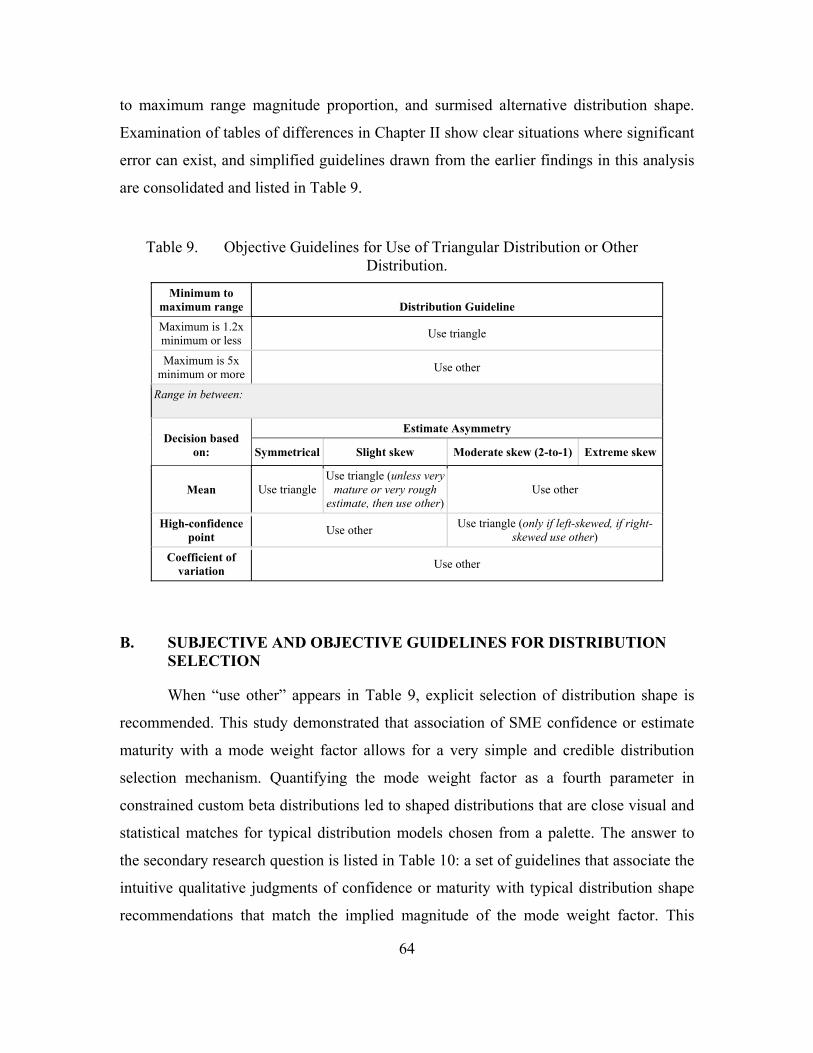
64
to maximum range magnitude proportion, and surmised alternative distribution shape.
Examination of tables of differences in Chapter II show clear situations where significant
error can exist, and simplified guidelines drawn from the earlier findings in this analysis
are consolidated and listed in Table 9.
Table 9. Objective Guidelines for Use of Triangular Distribution or Other Distribution.
Minimum to maximum range Distribution Guideline
Maximum is 1.2x minimum or less
Use triangle
Maximum is 5x minimum or more
Use other
Range in between:
Decision based on:
Estimate Asymmetry
Symmetrical Slight skew Moderate skew (2-to-1) Extreme skew
Mean Use triangle Use triangle (unless very
mature or very rough estimate, then use other)
Use other
High-confidence point
Use other Use triangle (only if left-skewed, if right-
skewed use other)
Coefficient of variation
Use other
B. SUBJECTIVE AND OBJECTIVE GUIDELINES FOR DISTRIBUTION SELECTION
When “use other” appears in Table 9, explicit selection of distribution shape is
recommended. This study demonstrated that association of SME confidence or estimate
maturity with a mode weight factor allows for a very simple and credible distribution
selection mechanism. Quantifying the mode weight factor as a fourth parameter in
constrained custom beta distributions led to shaped distributions that are close visual and
statistical matches for typical distribution models chosen from a palette. The answer to
the secondary research question is listed in Table 10: a set of guidelines that associate the
intuitive qualitative judgments of confidence or maturity with typical distribution shape
recommendations that match the implied magnitude of the mode weight factor. This

65
enables modelers to use the given three-point data with a simple fourth point to guide
distribution choice. If desired, the custom beta distribution accepts free-form use of the
mode weight d as a continuous variable instead of the discrete detent values matching
typical distribution shapes, which allows estimators to fine-tune peakedness in their
models.
Table 10. Subjective and Objective Guidelines for Distribution Selection.
Confidence in elicited
mode
Maturity of basis of estimate
Typical distribution
shape
Equivalent constrained custom beta
label
Custom beta constrained
shape parameter sum
Mode weight parameter (d) detent value
Very High VH Normal-3, Beta-n Beta-n 8 6
High H PERT Beta-p 6 4
Medium M Triangle Beta-t 5 3
Low L Beta-o Beta-o 2.5 0.5
Very Low VL Uniform Beta-u = =1 0
While the results of this study provide useful guidelines for any development
program using three-point estimates to make a step improvement in their modeling
practices, they are by no means the end point of analytical maturity in the area of three-
point estimate modeling, which is itself only a small segment of the domain of
uncertainty analysis. Topics for further research to extend the applicability of this study
in three-point estimate modeling include: 1) random survey of numerous three-point
estimates to determine frequency of cases matching categories in Table 9 guidelines; 2)
examination of whether mode weight tuning can be used to counter common elicitation
biases; 3) whether extending mode weight values d > 6 to produce still narrower
distribution shapes could match lognormal or other more specialized distribution models;
4) practicality and methods for Bayesian updating of three-point estimates modeled by
custom beta; 5) whether mode weight should drift with asymmetry rather than staying
constant; 6) validation studies to explicitly match broad user-base designations of
qualitative Likert scale values to exact d values rather than common typical shapes; and
7) whether qualitative scales in Table 9 are extensible to additional factors like degree of

66
technical challenge and plan aggressiveness to infer approximate three-point estimate
values from single point estimates.
When engineers and managers are called upon to make decisions under
uncertainty and a three-point estimate is the best data available, the data itself can
objectively guide modelers to use the distribution models that most accurately match the
state of the given information. Distribution shape selection can be crucial to the outcome
of the decision. While the simple triangular distribution is sufficient in many common
scenarios, observations about the provided three-point estimate data can identify
conditions when decision variables may be vulnerable to error and other distribution
shapes are better suited as models of uncertainty. When Table 9 estimate guidelines are
used in conjunction with pointers to Table 10 distribution selection criteria, an analyst is
well armed to quickly and easily go beyond the triangle to model and compute the most
accurate data possible in support of major development program decision makers.

67
APPENDIX: DISTRIBUTION EQUATIONS
Common distribution equations (Vose 2008, Appendix III.7).
Triangular distribution
( )
3
a b c
2 2 2( * * * )
18
a b c a b b c a c
Uniform distribution
( )
2
a c
2( )
12
c a
PERT distribution
( 4* )
6
a b c
( )*( )
7
a c
Beta distribution (4 parameter beta-general)
( 1)*( )
( 2)
c ab a
, if > 1, >1
*( )
( )
c aa
2
2
* *( )
( 1)*( )
c a

68
THIS PAGE INTENTIONALLY LEFT BLANK

69
LIST OF REFERENCES
Association for the Advancement of Cost Engineering, International. 2011. Cost Estimate Classification System. AACEI Recommended Practice No. 17R-91. Morgantown, WV: Association for the Advancement of Cost Engineering, International.
Boardman, Anthony E. 2006. Cost-benefit Analysis: Concepts and Practice. Upper Saddle River, NJ: Pearson/Prentice Hall.
Brown, Cinda L. 2008. Improved Methodology for Developing Cost Uncertainty Models for Naval Vessels. Monterey, CA: Naval Postgraduate School.
Cooke, Roger M. 1991. Experts in Uncertainty: Opinion and Subjective Probability in Science. New York, NY: Oxford University Press.
De Neufville, Richard, and Scholtes, Stefan. 2011. Flexibility in Engineering Design. Cambridge, MA: MIT Press.
Everitt, Brian S., and A. Skrondal. 1998. The Cambridge Dictionary of Statistics. 4th ed. Cambridge, UK: Cambridge University Press.
Hubbard, Douglas W. 2014. How to Measure Anything: Finding the Value of “Intangibles in Business.” 3rd ed. Hoboken, NJ: John Wiley and Sons, Inc.
Hulett, David T. 2009. Practical Schedule Risk Analysis. Burlington, VT: Gower Press.
Keefer, Donald L., and Bodily, Samuel E. 1983. “Three-Point Approximations for Continuous Random Variables.” Management Science 29(5): 595–609. http://dx.doi.org/10.1287/mnsc.29.5.595
Kujawski, E., Alvaro, M., and Edwards, W. 2004. “Incorporating psychological influences in probabilistic cost analysis.” Systems Engineering 7(3):195–216.
Moder, Joseph. J., and Rogers, E. G. 1968. “Judgment Estimates of the Moments of PERT Type Distributions.” Management Science 15(2):B76–B83.
National Aeronautics and Space Administration. 2007. NASA Systems Engineering Handbook. NASA Handbook No. NASA/SP-2007-6105, Rev. 1. Washington, DC: National Aeronautics and Space Administration.
Palisade Corporation. 2014. @Risk for Excel, Version 6.3.1 Industrial Edition. Ithaca, NY: Palisade Corporation. http://www.palisade.com/risk/.
Perry, C., and Greig, I. D. 1975. “Estimating the Mean and Variance of Subjective Distributions in PERT and Decision Analysis.” Management Science 21(12):1477-1480. http://dx.doi.org/10.1287/mnsc.21.12.1477

70
Project Management Institute. 2008. A Guide to the Project Management Body of Knowledge. 4th ed. PMBOK Guide, ANSI/PMI 99–001-2008. Newtown Square, PA: Project Management Institute, Inc.
U.S. Air Force. 2007. U.S. Air Force Cost Risk and Uncertainty Handbook. Hanscom AFB, Bedford, MA: Air Force Cost Analysis Agency.
U.S. Government Accountability Office. 2007. Cost Assessment Guide: Best Practices for Estimating and Managing Program Costs. GAO-07-1134SP. Washington, DC: U.S. Government Accountability Office.
Vose, David. 2008. Risk Analysis: A Quantitative Guide. 3rd ed. Chichester, West Sussex, UK: John Wiley & Sons, Ltd.
Yoon, Kwangsun, and Hwang, C. L. 1995. Multiple Attribute Decision Making: An Introduction. Thousand Oaks, CA: Sage Publications.

71
INITIAL DISTRIBUTION LIST
1. Defense Technical Information Center Ft. Belvoir, Virginia 2. Dudley Knox Library Naval Postgraduate School Monterey, California