Implementing the National Weather Service Global Workflow (GWF)

on the Azure CloudUsing the cloud to predict cloudiness

This work was part of the Azure HPC Collaboration Center funded by Microsoft in partnership with Intel.

Authors: Steve Bongiovanni • Andrew Qualkenbush • Chris Young • Don Avart

2

Table of Contents

1. Executive Summary .............................................................................................................................. 3

2. RedLine Lab .......................................................................................................................................... 5

2.1. Global Workflow Build and Configure - Redline HPC Lab ......................................................... 5

2.1.1. Operating System Choice ...................................................................................................... 5

2.1.2. Standard Linux Software Stack ............................................................................................. 5

2.1.3. RedLine Lab Configuration .................................................................................................. 6

2.1.4. Support Libraries and Applications for GWF ....................................................................... 6

2.2. Initial GWF Run Attempts ............................................................................................................ 8

2.3. Running GWF in the RedLine HPC Lab ...................................................................................... 9

3. Azure Setup ......................................................................................................................................... 10

3.1. Azure Lustre® Build and Test .................................................................................................... 10

3.2. Azure CycleCloud Setup and Test .............................................................................................. 11

3.3. Moving Global Workflow to Azure ............................................................................................ 13

4. Azure Execution .................................................................................................................................. 14

4.1. Running Low Resolution Forecast on Azure .............................................................................. 14

4.2. Increasing Forecast Resolution ................................................................................................... 14

4.3. Running at Full Resolution Using Only Publicly Available Data .............................................. 15

4.3.1. Cold Start Data from the NOAA NOMADS FTP Site ......................................................... 15

4.3.2. Warm Start Data from the NOAA AWS Data Store ............................................................ 16

4.3.3. Currently Insufficient Publicly Available Data for Full GWF Forecast Cycles ................. 16

5. Summary ............................................................................................................................................. 17

6. About RedLine .................................................................................................................................... 17

3

Implementing the National Weather Service

Global Workflow (GWF) on the Azure Cloud

1. Executive Summary

NOAA/NCEP’s Global Workflow (GWF) is a complex and interconnected series of batch jobs

that cycles through the global forecast system (GFS). Additional job steps include the analysis

(GSI), Hybrid EnKF (Ensemble Kalman Filter), POST and verification. The various components

have dependencies on other components of the workflow, all of which are controlled by one of

two workflow managers: ecFlow (when run in production) or Rocoto (when run by developers).

A flowchart and description of the steps can be found here: https://github.com/NOAA-

EMC/global-workflow/wiki/Global-Workflow-System-Jobs

In production, the GWF runs, or cycles, four times daily (00, 06, 12, and 18 UTC). In development,

it can be configured to run for a single cycle or, more often than not, 4 cycles a day to perform a

specific meteorological experiment or to develop future enhancements. These experiments and

enhancements are primarily run on a handful of systems either owned by or in cooperation with

NOAA. Access to these systems is limited to NOAA scientists and a relatively small number of

non-NOAA collaborators. These systems are physically limited to their existing hardware

resources, and individuals must receive the proper security credentials to gain access to some of

these systems. This unfortunately limits the amount of scientific and development work, as well

as collaboration, that can be accomplished. The ability to run the full GWF in the cloud opens

significant opportunities for NOAA to achieve the objectives of improving forecast skill and

testing new scientific algorithms from government, academic and commercial entities as being

envisioned by the establishment of NOAA's Earth Prediction Innovation Center (EPIC) and their

Big Data project to place more data in the cloud.

RedLine Performance Solutions (RedLine), working with Microsoft and Intel corporations, set out

to determine the feasibility of running the GWF in the Azure cloud. Our scope included building

all of the required executables and libraries, collecting and formatting the required data, and

cycling through a data assimilation loop to deliver the required input data to the GFS forecast

model, which produces forecast output. The forecast output from each cycle, along with current

observational data, feeds into the next forecast cycle. Achieving this goal of GWF operation on

Azure presented a number of challenges detailed throughout this paper. At a high level, two of the

most challenging aspects of the project were:

• Configuration: As stated above, the GWF is supported by NOAA on a select few

computing systems. Each of these systems are unique with a number of differences (e.g.,

4

parallel filesystems, job schedulers, processor configurations). The GWF, which is

accessible to the public on GitHub, assumes a standard configuration based on one of these

supported systems. To be best utilized by the public it needs to be more easily configured

and documentation improved.

• Data: There are two ways to start the GWF: a cold-start or warm-start. A warm-start means

that data from a previous cycle is used as input for the next cycle, while a cold-start

generally uses data that has been archived or created from a source other than the GWF

itself. Each of these methods requires specific data to be available. We are aware of two

locations that provide data for running the GWF: the NOAA public FTP site, inclusive of

NOMADS, and the NOAA Big Data project hosted by AWS. While neither site has all the

data required to either cold-start or warm-start the GWF, we had access to the additional

data needed.

The approach adopted for this project had three distinct steps:

• Step 1: Build and run the GWF in the RedLine lab. Building all of the code and running

at low resolution on lab resources avoids any charges against a fixed number of Azure

credits allotted by Microsoft while we worked through build and machine configuration

issues.

• Step 2: Build and test a parallel filesystem on the Azure cloud. Running the GWF requires

a robust parallel filesystem such as Lustre. Given that we did not have specific filesystem

requirements defined for the project, the approach was to define a base configuration for

Lustre and perform scaling tests to show linear scalability. We assumed we could scale to

a level that would meet our performance requirements.

• Step 3: Migrate data and executables to Azure and run GWF. Once GWF executables and

libraries had been built and tested in the lab, and a well-defined parallel filesystem was

established, integrating the components and running on Azure would be the final step.

Despite the challenges we encountered, we achieved our objectives, successfully cycling the GWF

through multiple iterations, at low-resolution and cold-starting the GWF at full-resolution on the

Azure cloud, opening doors to more collaboration and scientific innovation. The details of how

the executables and libraries were built, issues encountered and how they were resolved, and

ultimately the results of running GWF on the Azure cloud follow in the remainder of this paper.

5

2. RedLine Lab

RedLine decided to conserve the Azure resource allotment by initially building and executing the

Global Workflow in the RedLine lab.

2.1. Global Workflow Build and Configure - Redline HPC Lab

The Global Workflow is a collection of software that includes all applications required to produce

weather forecasts on a cycling basis. The GWF runs in production 4 times daily, using varying

resources, depending on the job that is running. In operations, the workflow has a highwater mark

of 800 Intel Broadwell (28 core) nodes. In development, it is used at varying resolutions, with

significantly fewer compute resources, to perform meteorological experiments and develop future

enhancements. NOAA uses a variety of machines in its production and development environments.

These machines use several different operating systems.

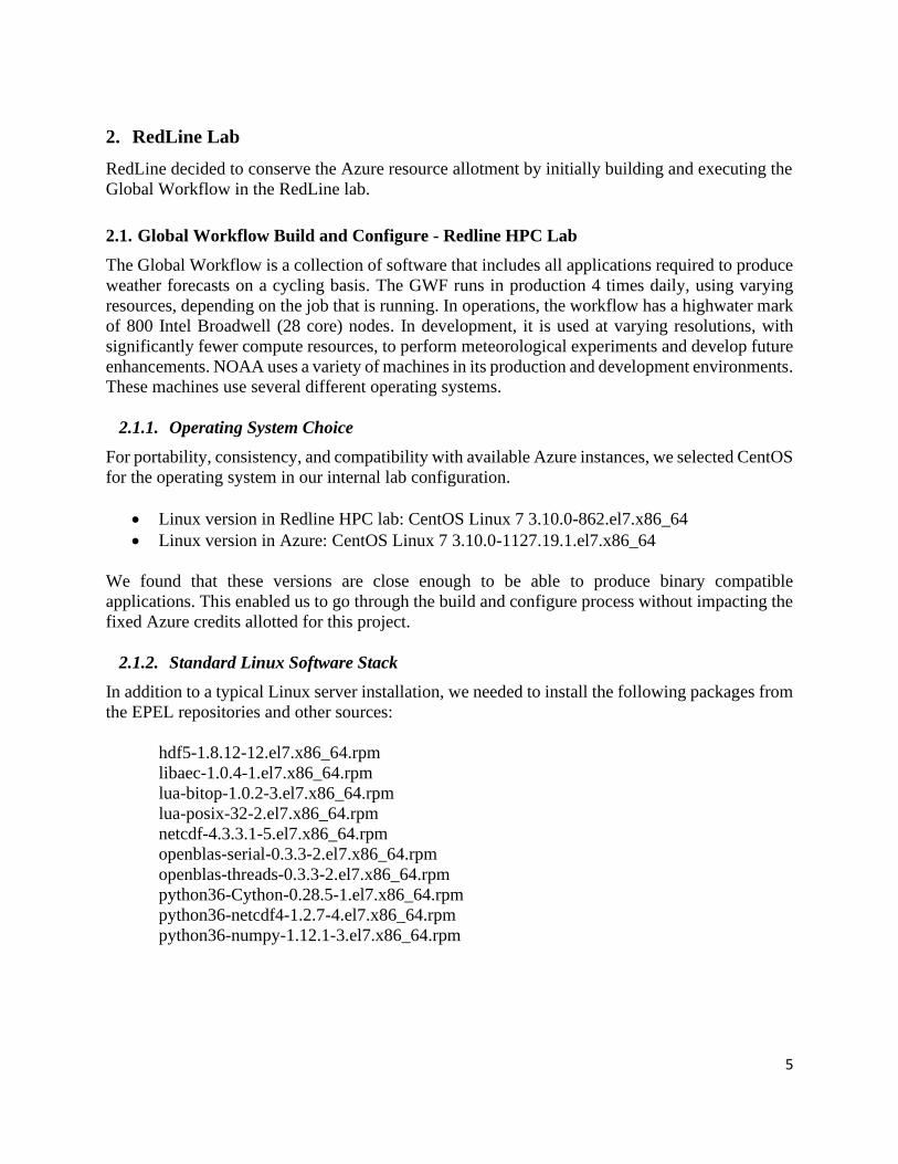
2.1.1. Operating System Choice

For portability, consistency, and compatibility with available Azure instances, we selected CentOS

for the operating system in our internal lab configuration.

• Linux version in Redline HPC lab: CentOS Linux 7 3.10.0-862.el7.x86_64

• Linux version in Azure: CentOS Linux 7 3.10.0-1127.19.1.el7.x86_64

We found that these versions are close enough to be able to produce binary compatible

applications. This enabled us to go through the build and configure process without impacting the

fixed Azure credits allotted for this project.

2.1.2. Standard Linux Software Stack

In addition to a typical Linux server installation, we needed to install the following packages from

the EPEL repositories and other sources:

hdf5-1.8.12-12.el7.x86_64.rpm

libaec-1.0.4-1.el7.x86_64.rpm

lua-bitop-1.0.2-3.el7.x86_64.rpm

lua-posix-32-2.el7.x86_64.rpm

netcdf-4.3.3.1-5.el7.x86_64.rpm

openblas-serial-0.3.3-2.el7.x86_64.rpm

openblas-threads-0.3.3-2.el7.x86_64.rpm

python36-Cython-0.28.5-1.el7.x86_64.rpm

python36-netcdf4-1.2.7-4.el7.x86_64.rpm

python36-numpy-1.12.1-3.el7.x86_64.rpm

6

In addition to the packages available in the standard repositories, we also directly downloaded and

installed:

● Spack - https://spack.io/

● LMOD (Lua Modules) - https://lmod.readthedocs.io/en/latest/

● Rocoto - http://christopherwharrop.github.io/rocoto/

Some of the build processes for GWF required newer versions of software than were available

from repositories. Using Spack, we built and installed the latest versions of the following packages:

● Ruby

● Python

● Cmake.

2.1.3. RedLine Lab Configuration

The Azure instance selected uses the Slurm Workload Manager. We adjusted the Redline Lab

Slurm configuration to match the Azure configuration, with the exception of some node

instantiation options that were specific to the Azure instance. The RedLine Lab consists of 24 Intel

Haswell compute nodes each with 2 Intel(R) Xeon(R) CPU E5-2680 v3 @ 2.50GHz and 128GB

RAM per node. Other features of the lab include a 28 TB Lustre parallel filesystem, Mellanox

FDR Infiniband high-speed interconnect, and the Slurm batch scheduler.

2.1.4. Support Libraries and Applications for GWF

The GWF is a diverse collection of applications written over a period of years by many individuals,

groups, and organizations. At various times during the process, different support libraries were

either popular, appropriate, or necessary. These support libraries came from several sources, but

over time many fell under the purview of NOAA. There have been several attempts to consolidate

these libraries, culminating in what is now referred to as hpc-stack, which is part of the NCEPLIBS

project. We selected hpc-stack for building the required GWF support libraries and applications.

2.1.4.1. HPC-STACK

Currently, all of the GWF library dependencies can be satisfied by the hpc-stack build process

and is exclusively being used by the UFS weather model (the core of the GFS) and the GWF now.

At the time the project was implemented, it did not appear that any of the then “configured” NCEP

machines made exclusive use of the hpc-stack build modules and libraries. They instead seemed

to use other pre-built versions of the required libraries in custom locations. To enhance portability

despite the unintended incompatibility amongst the “configured” machines, we opted to

consolidate all prerequisites for the GWF into a single path. As with the “build” portion of the

GWF, hpc-stack is a consolidation of numerous libraries and applications that have been brought

together under a single script-based build system. To the credit of those that developed this

system, it worked very well. We easily built the requisite libraries with both Intel ics/2018.4 and

Intel ics/2020.0 compiler suites. The main web location for hpc-stack is on github:

https://github.com/NOAA-EMC/hpc-stack.

7

HPC-STACK components used in this project:

NCEPLIBS Third Party Libraries

● NCEPLIBS-bacio ● NCEPLIBS-sigio ● NCEPLIBS-sfcio ● NCEPLIBS-gfsio ● NCEPLIBS-w3nco ● NCEPLIBS-sp ● NCEPLIBS-ip ● NCEPLIBS-ip2 ● NCEPLIBS-g2 ● NCEPLIBS-g2c ● NCEPLIBS-g2tmpl ● NCEPLIBS-nemsio ● NCEPLIBS-nemsiogfs ● NCEPLIBS-w3emc ● NCEPLIBS-landsfcutil ● NCEPLIBS-bufr ● NCEPLIBS-wgrib2 ● NCEPLIBS-prod_util ● NCEPLIBS-grib_util ● NCEPLIBS-ncio ● NCEPLIBS-wrf_io ● EMC_crtm ● EMC_post

● udunits ● PNG ● JPEG ● Jasper ● SZip ● Zlib ● HDF5 ● PNetCDF ● NetCDF ● ParallelIO ● nccmp ● nco ● CDO ● FFTW ● GPTL ● Tau2 ● Boost ● Eigen

2.1.4.2. Global Workflow Software Stack

The diversity of GWF applications, tools, and languages used makes the task of creating a unified

script-based build environment very difficult. There are a variety of build paradigms from simple

shell-based build scripts, to conventional makefile-based builds, to Cmake-based builds, all under

the control of a set of high-level shell scripts. Making this task even more challenging is the process

of making this future-compatible. GWF pulls or clones particular versions of the various

applications during the build process. With multiple git subprojects, tracking changes made to

facilitate our build was very difficult as the subdirectories were subject to different git repositories.

To make changes to the GWF, one needs to push changes to many different projects and git

repositories. This significantly complicated tracking changes we made to the GWF for this project.

8

We were able to establish the essential specifications of the “configured” machines to determine

which one most closely matched our configuration and was the most generic. We opted to use that

as our model for the code modifications required to do the porting to the RedLine Lab environment.

This might not seem like it should be a requirement, but the GWF code is infused with very specific

“special case code” that is unique to each of the machines. In some cases, it operates by checking

hostnames and in other cases, by checking the existence of a particular filesystem path - which is

assumed to be unique. Given this method of the prior “porting,” it is not hard to imagine the

difficulties encountered in doing a new “port.” Nearly 120 files needed to be changed or created

anew to facilitate the GWF build process.

We experimented with potential schemes to simplify the porting process by “externalizing” much

of the machine-specific configurations. This included applying the LMOD collection capability to

allow upgrades to module versions without editing tens of files if support libraries were updated.

We also created a single highest-level run script to define and map the needed environment

variables, module versions, and compiler arguments. However, we encountered apparent

shortcomings in the LMOD collection feature that prevented conditional redefinition of

environment variables in module files. After many iterations, and under significant time

constraints, we elected to abandon the porting process simplifications.

At the time the project was implemented, none of the NOAA supported machines make exclusive

use of the hpc-stack built libraries and applications, but instead have locally built versions of the

support libraries in different locations. Given that none of the GWF predefined configurations for

the supported machines seemed to work using only hpc-stack out of the box, significant effort was

required to integrate the hpc-stack versions of all the libraries with GWF. However, this effort was

worthwhile as it will greatly simplify running GWF in the cloud. Given that there is still no uniform

specification regarding which environment variables are defined in the different hpc-stack module

files, and there is a similar situation on the GWF side with its build process requiring different

environment variables, we needed to experimentally and iteratively determine the required

mapping from what was defined by hpc- stack to what was required by the GWF. Our objective

was to determine the viability of running the GWF outside of the configured NOAA environment

and that part of the project proved to be difficult.

However, we were eventually able to overcome these challenges and did complete the build of the

entire GWF in our “generic” Linux environment.

2.2. Initial GWF Run Attempts

After the build was completed, we moved to the testing phase of the project. This involved

configuring the running environment with the specific configuration of our cluster and gathering

the necessary data to perform a complete forecast cycle. We anticipated some difficulty in this

process. As we worked through the porting process, it became clear the differently configured

machines kept their required input and static data in different locations. This static data

requirement does not seem to be documented anywhere. The initial iterations in this regard were

slow as it took time to identify what the static data was and subsequently obtain it. The GWF run

scripts used by the Rocoto workload manager are well-instrumented, most of them have shell

tracing enabled, which makes tracking backward to determine failure causes straightforward.

9

Once we worked through the failures in the run scripts caused by the missing data, we were able

to start running the GWF applications. This started well, but we quickly encountered some

segmentation faults dealing with GDAS/ENKF (Global Data Assimilation System/Ensemble

Kalman Filter). After extensive experimentation and investigation, we learned that NOAA has not

yet upgraded to the Intel 2020.0 compiler suite on their supported machines and that it was not

officially supported by the GWF. To the best of our knowledge, we were the first to attempt to

build with this version. Since debugging GDAS/ENKF was not in the scope for this project, we

opted to roll back to the 2018.4 version of the Intel compiler suite. The downgrade went perfectly

smoothly and only required a redefinition of a few environment variables in our highest-level build

scripts to rebuild both the hpc-stack and the GWF. With this new build, we had no further issues

with application failures of this nature.

2.3. Running GWF in the RedLine HPC Lab

In our lab environment, we utilized a 24-node cluster and ran the GWF at a low resolution

(C192/C96). We had some issues with the initial node configuration since the naming of some

settings in the configuration files was not obvious. We were able to do a cold-start run at this

resolution in the lab. What follows is a portion of a ‘rocotostat’ output for our test run in the

RedLine Lab environment:

CYCLE TASK JOBID STATE EXIT STATUS TRIES DURATION

===============================================================================================================================

202009011800 gdasfcst 5508 SUCCEEDED 0 1 371.0

202009011800 gdaspost000 5519 SUCCEEDED 0 1 301.0

202009011800 gdaspost001 5520 SUCCEEDED 0 1 193.0

202009011800 gdaspost002 5521 SUCCEEDED 0 1 196.0

202009011800 gdaspost003 5522 SUCCEEDED 0 1 194.0

202009011800 gdaspost004 5523 SUCCEEDED 0 1 196.0

202009011800 gdaspost005 5524 SUCCEEDED 0 1 189.0

202009011800 gdaspost006 5525 SUCCEEDED 0 1 196.0

202009011800 gdaspost007 5526 SUCCEEDED 0 1 189.0

202009011800 gdaspost008 5527 SUCCEEDED 0 1 196.0

202009011800 gdaspost009 5528 SUCCEEDED 0 1 187.0

202009011800 gdaspost010 5529 SUCCEEDED 0 1 197.0

Getting to the point of being able to run sequential full cycles did require several iterations and

restarts to figure out some of the “quirks” of the Rocoto workflow manager.

10

3. Azure Setup

Once we had a stable, successful GWF build and execution in the RedLine lab, we built the Azure

environment.

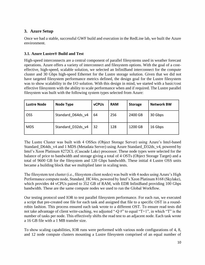
3.1. Azure Lustre® Build and Test

High-speed interconnects are a central component of parallel filesystems used in weather forecast

operations. Azure offers a variety of interconnect and filesystem options. With the goal of a cost-

effective, high-speed, scalable solution, we selected an InfiniBand interconnect for the compute

cluster and 30 Gbps high-speed Ethernet for the Lustre storage solution. Given that we did not

have targeted filesystem performance metrics defined, the design goal for the Lustre filesystem

was to show scalability in the I/O solution. With this design in mind, we started with a basic/cost

effective filesystem with the ability to scale performance when and if required. The Lustre parallel

filesystem was built with the following system types selected from Azure:

Lustre Node Node Type vCPUs RAM Storage Network BW

OSS Standard_D64ds_v4 64 256 2400 GB 30 Gbps

MDS Standard_D32ds_v4 32 128 1200 GB 16 Gbps

The Lustre Cluster was built with 4 OSSes (Object Storage Server) using Azure’s Intel-based

Standard_D64ds_v4 and 1 MDS (Metadata Server) using Azure Standard_D32ds_v4, powered by

Intel’s Xeon Platinum 8272CL (Cascade Lake) processor. These node types were selected for the

balance of price to bandwidth and storage giving a total of 4 OSTs (Object Storage Target) and a

total of 9600 GB for the filesystem and 120 Gbps bandwidth. These initial 4 Lustre OSS units

became a building block that we multiplied later in scaling tests.

The filesystem test cluster (i.e., filesystem client nodes) was built with 4 nodes using Azure’s High

Performance compute node, Standard_HC44rs, powered by Intel’s Xeon Platinum 8168 (Skylake),

which provides 44 vCPUs paired to 352 GB of RAM, with EDR InfiniBand providing 100 Gbps

bandwidth. These are the same compute nodes we used to run the Global Workflow.

Our testing protocol used IOR to test parallel filesystem performance. For each run, we executed

a script that pre-created one file for each task and assigned that file to a specific OST in a round-

robin fashion. This process ensured each task wrote to a different OST. To ensure read tests did

not take advantage of client write-caching, we adjusted “-Q #” to equal “T+1”, in which “T” is the

number of tasks per node. This effectively shifts the read test to an adjacent node. Each task wrote

a 16 GB file with a 1 MB transfer size.

To show scaling capabilities, IOR runs were performed with various node configurations of 4, 8,

and 12 node compute clusters mounting a Lustre filesystem comprised of an equal number of

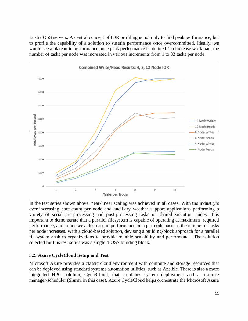
11

Lustre OSS servers. A central concept of IOR profiling is not only to find peak performance, but

to profile the capability of a solution to sustain performance once overcommitted. Ideally, we

would see a plateau in performance once peak performance is attained. To increase workload, the

number of tasks per node was increased in various increments from 1 to 32 tasks per node.

In the test series shown above, near-linear scaling was achieved in all cases. With the industry’s

ever-increasing core-count per node and ancillary weather support applications performing a

variety of serial pre-processing and post-processing tasks on shared-execution nodes, it is

important to demonstrate that a parallel filesystem is capable of operating at maximum required

performance, and to not see a decrease in performance on a per-node basis as the number of tasks

per node increases. With a cloud-based solution, devising a building-block approach for a parallel

filesystem enables organizations to provide reliable scalability and performance. The solution

selected for this test series was a single 4-OSS building block.

3.2. Azure CycleCloud Setup and Test

Microsoft Azure provides a classic cloud environment with compute and storage resources that

can be deployed using standard systems automation utilities, such as Ansible. There is also a more

integrated HPC solution, CycleCloud, that combines system deployment and a resource

manager/scheduler (Slurm, in this case). Azure CycleCloud helps orchestrate the Microsoft Azure

12

infrastructure to auto-scale compute resources as needed. It integrates with most popular

schedulers to keep the user/researcher/scientist job submission process the same.

CycleCloud was used to deploy the clusters in this project, for both the Slurm compute and the

Lustre filesystem cluster outlined above. CycleCloud required a server to be built (Standard D3 v2

VM, (Virtual Machine) was selected) in the Azure environment, that interacted with the Azure

API to deploy and configure servers into a Slurm cluster. Once the CycleCloud server was

deployed, a browser or the CycleCloud CLI could be used to interact with the CycleCloud

application.

CycleCloud included a variety of built-in templates for different schedulers and filesystems, but

we used customized templates for both of our deployed clusters. The Slurm template was

customized to provide support for mounting a Lustre filesystem, while the Lustre filesystem

template was customized to support the hardware configuration we decided to use for the Lustre

environment. This was required since the standard “LFS Community” template did not support the

specific disk attached to the VMs. It also needed customization to start a separate HSM

(Hierarchical Storage Management) node instead of running this function on the MDS in the

cluster. The HSM node was required to enable push and pull of the Lustre filesystem data to blob

storage so the Lustre cluster can be shut down when not needed, but the data can be easily restored

when it is re-deployed.

The Slurm cluster had the option of using standard images for the head node and compute nodes,

but we created a customized version of a Centos 7.7 HPC-based image available in Azure. The

customized Slurm template installed Lustre client packages on the nodes as they are deployed, but

we installed these and other needed packages into our image. This has the added benefit of

speeding up the node deployment process, since these customizations do not have to be performed

on every node at deployment time. We used the following software stack on the Slurm cluster:

• CentOS Linux release 7.7.1908 (kernel - 3.10.0-1127.19.1.el7.x86_64)

• Mellanox OFED-5.2-1.0.4

• Lustre client 2.12.5.

The HC44 VM was chosen for both head node and compute nodes and consists of:

• 44 Intel Xeon Platinum 8168 processor cores

• 8 GB of RAM per CPU core

• No hyperthreading

• AVX-512 extensions

• 100 Gb/sec Mellanox EDR InfiniBand.

When the CycleCloud cluster was started, a head node was deployed and configured as a Slurm

master. The CycleCloud deployment process generated a Slurm configuration with references for

the future compute nodes expected to be placed into service. This expected node count is calculated

from the “Max HPC Cores” configuration item in the Slurm template and requires a cluster restart

to modify. The compute nodes could either be started manually from the CycleCloud web or CLI

interfaces, or started when a user submitted a job. An idle time could be set to stop the nodes if a

13

job had not been run on them in a certain period of time or they could also be stopped manually

via the CycleCloud web interface or command line. We manually started and stopped compute

resources in the Slurm cluster, and excluded our Slurm partition from terminating nodes after a

pre-defined idle time. This allowed us to better control cost/usage of the nodes and enabled easier

debugging of application runtime issues.

An important configuration item to note is the “VM Scale Set” limit in CycleCloud. By default, it

only permits CycleCloud to run 100 VMs, too few for our test. We opened a support ticket with

Azure to increase this limit to 300 VMs.

CycleCloud had basic user and group configuration options to add userids (including ssh keys)

and groups that would be added to all of the nodes on deployment. This negated the need to add

any user/group information in the image itself. Once the CycleCloud cluster was deployed, users

could log into the head node using their own user accounts (password or public key authentication)

to compile code, submit jobs, etc. Once deployed, the cluster would be recognizable and

comfortable for users with a general HPC background.

3.3. Moving Global Workflow to Azure

To make our implementation and deployment of the GWF as portable as possible, we opted to

force the entire workflow including builds, installations, support data, input data and run

directories into a single directory tree. This simplified the process of moving the workflow from

the RedLine lab to Azure. Since we had binary compatibility, we could confidently copy that single

directory tree to the parallel filesystem we had configured on Azure, make some minor changes to

the system shell setup scripts, and run in place. If the Azure cluster had a different chip architecture

than our lab, the process of rebuilding for an alternate architecture would be a straightforward

process with the changes we had made to the build scripts.

Once we had the Lustre filesystem running (see below for a detailed description), we simply

synchronized our single directory tree between the lab and Azure using ‘rsync.’ We took care to

preserve symbolic links, which are used heavily in the GWF and LMOD, as well as other packages

in the tree.

We encountered some unexpected behavior when saving our Lustre filesystem to a “blob” in

Azure. In some cases, file ownership was lost and some symbolic links were broken. This was

easily fixed with a second ‘rsync’ command from the Redline Lab and a simple reinstallation of

the Intel compiler suite. The total size of the GWF and the low-resolution data was about 240GB.

14

4. Azure Execution

Once we created the Azure environment and migrated the GWF from the RedLine lab to Azure,

we were ready to run the GWF at first low-, then at the operational resolution.

4.1. Running Low Resolution Forecast on Azure

After the move to Azure and working out the few issues we encountered in that process, we were

able to rerun the low resolution forecasts with no issues. Given that we did not change the

resolution, and the configuration of the nodes was similar, we re-used the same configuration from

the RedLine lab in the Azure environment and instantiated a 24-node cluster to mimic what we

used in the lab.

On “spinning up” the cluster in Azure, we noted several issues that we expect will be resolved in

the future on Azure. The time to bring up the cluster was longer than expected, ranging from 5 to

15 minutes. We also found that nodes occasionally did not complete the configuration phase of the

startup, requiring a terminate-node action and subsequent restart before the node was available as

part of the cluster. We also occasionally observed the entire cluster become available, only to

immediately and spontaneously self-terminate. However, once all the nodes in the cluster were up

and running, we had no further problems with either stability, availability, or performance.

Given that we had a known working configuration for GWF with all required data for the low-

resolution run, we were able to repeat our lab run on Azure with similar results. Due to the limited

Azure budget, we shut down the cluster to work on preparing for a full-resolution run once we

confirmed the ability to run a single cycle at low resolution.

4.2. Increasing Forecast Resolution

The next step in the process was to increase the resolution to (C768/C384) using a maximum of

150 nodes, 44 cores each for a total of 6600 processors, and run that full resolution forecast on

Azure. To run at this resolution, we needed to gather not only the full resolution startup and input

data but also additional corresponding support data at that resolution. We were able to obtain the

cold-start data, subsequent observational input data, and the support data required to run at full

resolution. Using this data, we were able to “cycle” the GWF at full resolution. We did encounter

some of the same “quirks” in running via Rocoto that were resolved by reinitializing its internal

run database. What follows is a portion of a ‘rocotostat’ for our first successful run of GWF at full

resolution on the Azure platform. It can be seen that this is a clean run with exit statuses of zero

and only a single attempt at execution for each application.

SUCCESSFUL FULL RESOLUTION CYCLE CYCLE TASK JOBID STATE EXIT STATUS TRIES DURATION

================================================================================================================================

202103021800 gdasfcst 128 SUCCEEDED 0 1 2254.0

202103021800 gdaspost000 148 SUCCEEDED 0 1 304.0

202103021800 gdaspost001 139 SUCCEEDED 0 1 289.0

202103021800 gdaspost002 140 SUCCEEDED 0 1 314.0

202103021800 gdaspost003 141 SUCCEEDED 0 1 294.0

202103021800 gdaspost004 142 SUCCEEDED 0 1 305.0

202103021800 gdaspost005 143 SUCCEEDED 0 1 317.0

15

202103021800 gdaspost006 144 SUCCEEDED 0 1 299.0

202103021800 gdaspost007 145 SUCCEEDED 0 1 304.0

202103021800 gdaspost008 146 SUCCEEDED 0 1 314.0

202103021800 gdaspost009 147 SUCCEEDED 0 1 296.0

202103021800 gdaspost010 149 SUCCEEDED 0 1 305.0

202103021800 gdasvrfy 150 SUCCEEDED 0 1 7.0

202103021800 gdasarch 151 SUCCEEDED 0 1 5.0

202103021800 gdasefcs02 130 SUCCEEDED 0 1 2248.0

202103021800 gdasefcs03 131 SUCCEEDED 0 1 2244.0

202103021800 gdasefcs04 132 SUCCEEDED 0 1 2272.0

202103021800 gdasefcs05 133 SUCCEEDED 0 1 2273.0

202103021800 gdasefcs06 134 SUCCEEDED 0 1 2279.0

202103021800 gdasefcs07 135 SUCCEEDED 0 1 2225.0

202103021800 gdasefcs08 136 SUCCEEDED 0 1 2230.0

202103021800 gdasefcs09 137 SUCCEEDED 0 1 2239.0

202103021800 gdasefcs10 138 SUCCEEDED 0 1 2217.0

202103021800 gdasechgres 152 SUCCEEDED 0 1 205.0

202103021800 gdasepos000 153 SUCCEEDED 0 1 466.0

202103021800 gdasepos001 154 SUCCEEDED 0 1 467.0

4.3. Running at Full Resolution Using Only Publicly Available Data

Since a secondary objective of this project was to establish the viability of running GWF on Azure

using only publicly available input data, we attempted to start a new forecast run using only this

data. The primary data stores used by NOAA that are intended to provide the required data for

GWF runs are:

• NOMADS - https://ftp.ncep.noaa.gov/data/nccf/com/gfs/prod/

• AWS S3 Data Store - noaa-gfs-warmstart-pds.s3.amazonaws.com

4.3.1. Cold Start Data from the NOAA NOMADS FTP Site

We referenced the NOMADS (NOAA Operational Model Archive and Distribution System)

website, which makes non-restricted data for running GWF at full scale available to the public for

research and collaboration purposes. Using the available documentation as a guide, we set out to

initialize and run a new forecast cycle using only this publicly available data. Due to the volume

of the “cold-start” portion of the data, specifically the ENKF/GDAS data, NOAA only retains data

for the prior 4 cycles. The NOMADS site has somewhat limited bandwidth, and throttles access to

a single IP address that has heavy usage and eventually will block that IP address if there are too

many requests or connections in a short period of time. This caused unexpected delays in

downloading the required data. Unfortunately, we opted to start pulling the GFS data first, but by

the time its download completed, the ENKF data cycle we needed had rolled off the system,

requiring us to download the GFS data again to match the ENKF data that was then available.

On attempting to start a forecast using only this data, we quickly realized that not all of the required

data was available on the NOMADS site. We discovered there might be some workarounds that

we could attempt (e.g., renaming certain files, in some cases using the “wrong” files to fill in the

cold-start data). The workarounds would allow the model to run, but would impact the first few

cycle’s forecast results. This was a long, iterative, and somewhat tedious process, that in the end

was unsuccessful. It might not be impossible, but it was impractical given our time constraints.

16

4.3.2. Warm Start Data from the NOAA AWS Data Store

NOAA also has a big data initiative in which other data is being provided to the public via multiple

AWS S3 data stores. The data located here is different from that on the NOMADS site. This site

includes “warm-start” data to bootstrap a forecast cycle based on the output of a prior run.

However, at the time we attempted the run it did not appear that this site had all of the data needed

to do a complete forecast cycle. It was an iterative process to attempt a forecast cycle using only

this data. We were informed that at one point all of the required data for a restart was on the site,

but it was not clear that it had ever been run on anything other than a NOAA-configured machine,

which typically has other required run data or direct access to the remainder of the required data

already available in its local file systems. It is possible that the version of GWF that we were using,

which was the latest version as of May 2021, may require a different data layout or different files

than a prior version which might have run in the past. At this time, we were unable to achieve a

successful run using only the data available on the AWS data store but we are confident that NOAA

will address these issues in the future.

4.3.3. Currently Insufficient Publicly Available Data for Full GWF Forecast Cycles

In the end, we were unable to achieve a complete successful run using only publicly available data

sources. This does not mean that it is impossible, or that there might be other data of which we are

unaware, but to the best of our knowledge, the current data is insufficient. This is by no means a

permanent condition, as NOAA is actively engaged in collaboration efforts and is aware of these

limitations.

17

5. Summary

The magnitude of the various efforts by many people at NOAA and elsewhere should not be

underestimated. To unify a build process for diverse code bases for a wide variety of applications

is a significant undertaking. We applaud the efforts of NOAA and others in this regard. There are

still areas that can be improved in the GWF build process to ease this effort, especially related to

consolidating all machine-specific code to a unified location. Even this, which sounds simple, is

complicated by the fact that the changes need to be made in a way that would not adversely affect

the integrity of the stand-alone build processes of the component applications.

Regardless of these various difficulties, our goal was to assess the viability of running full

resolution weather forecasts on the Azure platform. To that end, this was a major success. We were

able to “port” the code to machines that are not NOAA-maintained and we were able to

successfully run full resolution weather forecasts on the Azure platform.

6. About RedLine

RedLine has been working with National Weather Service (NWS) and National Centers for

Environmental Prediction (NCEP) for over 20 years on both the operational and research high

performance computing contracts, administration of operational workflows, and scientific support

development. We have optimized the models at both the hardware and software levels, helped

establish the NGGPS (Next Generation Global Prediction System), are participating in the JEDI

(Joint Effort for Data assimilation Integration) project to develop the next generation data

assimilation system and contributed to the NOAA RDHPCS cloud pilot study. Our RedLine team

continues to staff HPC operations on the WCOSS II (Weather and Climate Operational

Supercomputing System) contract and will be supporting NOAA on the recently awarded EPIC

contract. RedLine’s unique experience gives us insight into how the models are developed and

implemented into operations, and how this process for research to operations could be managed in

a more unified modeling environment.