implementation and refinement techniques for abstract

Refinement andImplementation Techniques

forAbstract State Machines

Dissertationzur Erlangung des Grades eines Doktorsder Naturwissenschaften (Dr. rer. nat.)

im Fachbereich Informatikder Universitat Ulm

vorgelegt von

Joachim Schmid

aus Tuttlingen

Abteilung fur Programmiermethodik und Compilerbau(Leiter: Prof. Dr. Helmuth Partsch)

2002

II

Amtierender Dekan: Prof. Dr. Gunther Palm

Gutachter: Prof. Dr. Helmuth Partsch (Universitat Ulm)Prof. Dr. Friedrich von Henke (Universitat Ulm)Prof. Dr. Egon Borger (Universitat Pisa)

Tag der Prufung: 17. Juni 2002

Danksagung

An dieser Stelle mochte ich mich bei allen Personen bedanken, die mich bei derErstellung dieser Arbeit unterstutzt haben.

Besonderen Dank gilt Herrn Prof. Dr. Egon Borger, der stets ein offenesOhr fur Fragen und Diskussionen hatte und mich zu dieser Arbeit motivierte.

Bedanken mochte ich mich fur die tatkraftige Unterstutzung durch Dr. PeterPappinghaus, der meine Promotion bei der Siemens AG betreute. Dank giltauch allen anderen Mitarbeitern von CT SE 4, welche manchmal von ihrerArbeit abgehalten wurden.

Dank gilt der Siemens AG, die mir die notwendigen Arbeitsmittel zur Verfu-gung stellte und mich finanziell unterstuzte. Insbesondere mochte ich mich beidem Fachzentrumsleiter Prof. Dr. Wolfram Buttner bedanken, der sich bereiterklart hatte, diese Dissertation durch die Siemens AG zu unterstutzen.

III

Contents

Introduction 1

1 Submachine Concept 31.1 Standard ASMs . . . . . . . . . . . . . . . . . . . . . . . . . . . . 41.2 Sequential Composition and Iteration . . . . . . . . . . . . . . . 5

1.2.1 Sequence Constructor . . . . . . . . . . . . . . . . . . . . 61.2.2 Iteration Constructor . . . . . . . . . . . . . . . . . . . . 81.2.3 Bohm-Jacopini ASMs . . . . . . . . . . . . . . . . . . . . 10

1.3 Parameterized Machines . . . . . . . . . . . . . . . . . . . . . . . 131.4 Further Concepts . . . . . . . . . . . . . . . . . . . . . . . . . . . 15

1.4.1 Local State . . . . . . . . . . . . . . . . . . . . . . . . . . 151.4.2 ASMs with Return Value . . . . . . . . . . . . . . . . . . 161.4.3 Error Handling . . . . . . . . . . . . . . . . . . . . . . . . 17

1.5 Related Work . . . . . . . . . . . . . . . . . . . . . . . . . . . . . 17

2 Component Concept 192.1 Component . . . . . . . . . . . . . . . . . . . . . . . . . . . . . . 20

2.1.1 Formal Definition . . . . . . . . . . . . . . . . . . . . . . . 202.1.2 Abstraction . . . . . . . . . . . . . . . . . . . . . . . . . . 232.1.3 Verification . . . . . . . . . . . . . . . . . . . . . . . . . . 232.1.4 Defining Components . . . . . . . . . . . . . . . . . . . . 25

2.2 Composition of Components . . . . . . . . . . . . . . . . . . . . . 312.2.1 Formal Definition . . . . . . . . . . . . . . . . . . . . . . . 312.2.2 Defining Composition . . . . . . . . . . . . . . . . . . . . 37

2.3 Component based Verification . . . . . . . . . . . . . . . . . . . . 412.4 Related Work . . . . . . . . . . . . . . . . . . . . . . . . . . . . . 49

3 Execution of Abstract State Machines 513.1 Functional Programming and ASMs . . . . . . . . . . . . . . . . 513.2 Lazy Evaluation . . . . . . . . . . . . . . . . . . . . . . . . . . . 523.3 Lazy Evaluation and ASMs . . . . . . . . . . . . . . . . . . . . . 54

3.3.1 Nullary Dynamic Functions . . . . . . . . . . . . . . . . . 543.3.2 Firing Rules . . . . . . . . . . . . . . . . . . . . . . . . . . 563.3.3 Unary Dynamic Functions . . . . . . . . . . . . . . . . . . 573.3.4 Referential Transparency . . . . . . . . . . . . . . . . . . 59

3.4 Sequential Execution of Rules . . . . . . . . . . . . . . . . . . . . 623.5 Related Work . . . . . . . . . . . . . . . . . . . . . . . . . . . . . 64

V

VI CONTENTS

4 The AsmGofer System 654.1 The Interpreter . . . . . . . . . . . . . . . . . . . . . . . . . . . . 65

4.1.1 Expression Evaluation . . . . . . . . . . . . . . . . . . . . 664.1.2 Dealing with Files . . . . . . . . . . . . . . . . . . . . . . 664.1.3 Other Commands . . . . . . . . . . . . . . . . . . . . . . 67

4.2 Sequential ASMs . . . . . . . . . . . . . . . . . . . . . . . . . . . 674.2.1 Nullary Dynamic Functions . . . . . . . . . . . . . . . . . 684.2.2 Unary Dynamic Functions . . . . . . . . . . . . . . . . . . 704.2.3 Update Operator . . . . . . . . . . . . . . . . . . . . . . . 714.2.4 N-ary Dynamic Functions . . . . . . . . . . . . . . . . . . 714.2.5 Execution of Rules . . . . . . . . . . . . . . . . . . . . . . 724.2.6 Rule Combinators . . . . . . . . . . . . . . . . . . . . . . 73

4.3 Distributed ASMs . . . . . . . . . . . . . . . . . . . . . . . . . . 744.4 An Example: Game of Life . . . . . . . . . . . . . . . . . . . . . 76

4.4.1 Static Semantics . . . . . . . . . . . . . . . . . . . . . . . 764.4.2 Dynamic Semantics . . . . . . . . . . . . . . . . . . . . . 78

4.5 Automatic GUI Generation . . . . . . . . . . . . . . . . . . . . . 794.6 User defined GUI . . . . . . . . . . . . . . . . . . . . . . . . . . . 81

5 Applications 855.1 The Light Control System . . . . . . . . . . . . . . . . . . . . . . 855.2 Java and the Java Virtual Machine . . . . . . . . . . . . . . . . . 855.3 Hardware Verification . . . . . . . . . . . . . . . . . . . . . . . . 865.4 FALKO . . . . . . . . . . . . . . . . . . . . . . . . . . . . . . . . 87

Conclusions and Outlook 89

Zusammenfassung 93

Appendix 95

A Submachine Concept 95A.1 Deduction Rules for Update Sets . . . . . . . . . . . . . . . . . . 95

B Component Concept 99B.1 Syntax . . . . . . . . . . . . . . . . . . . . . . . . . . . . . . . . . 99B.2 Semantics . . . . . . . . . . . . . . . . . . . . . . . . . . . . . . . 100B.3 Type system . . . . . . . . . . . . . . . . . . . . . . . . . . . . . 102B.4 Constraints . . . . . . . . . . . . . . . . . . . . . . . . . . . . . . 104

References 105

Introduction

The notion of Abstract State Machines (ASMs), defined by Gurevich in [33, 34],has been used successfully for the design and the analysis of numerous complexsoftware and hardware systems (see [16] for an overview). The outstandingfeatures which are responsible for this success are the simple yet most generalnotion of state—namely mathematical structures, providing arbitrary abstractdata types—together with the simultaneous execution of multiple atomic actionsas the notion of state transforming basic machine step.

This view, of multiple atomic actions executed in parallel in a common state,comes however at a price: the standard composition and structuring principles,which are needed for high-level system design and programming in the large,are not directly supported and can be introduced only as refinement steps. Alsothe freedom in the choice of the appropriate data structures, which provides apowerful mechanism to describe systems at various levels of abstraction, has aprice: it implies an additional step to turn these abstractions into executablemodels, so that experimental validation can be done via simulation.

In this thesis we enhance the usefulness of ASMs for software engineeringpractice by:

• defining three major composition concepts for ASMs, namely componentmachine, parameterized submachine, and iteration, which cannot be dis-pensed with in software engineering (Chap. 1, Chap. 2)

• developing a tool that allows to execute these extended ASMs and comeswith a graphical user interface, to support experimental analysis (Chap. 3,Chap. 4)

We have tested the practicality of the proposed concepts and of their implemen-tation (Chap. 5), namely by the design and the analysis

• of a well-known software engineering case study in the literature and of amiddle sized industrial software development project (for a train timetableconstruction and validation system). This project work also included thedevelopment of a proprietary compiler from ASMs to C++.

• of the Java language and its implementation on the Java Virtual Machine

• of an industrial ASIC design and verification project. This project workalso included the development of a compiler from ASM components toVHDL.

Part of this work has been published already in [17, 18, 19, 61, 63, 64].

1

2 Introduction

Notational conventions

Throughout this thesis we stick to standard mathematical terminology. Never-theless, we list here some frequently used notations.

We write P(X ) for the set of all subsets of X .

We write X � f for the domain restriction of the function f to the set X :

X � f := {(x , f (x )) | x ∈ dom(f ) ∩X }

We use ε for the empty sequence and · to separate elements in a sequence.Further, we write R≥n for the universe containing all sequences of R with lengthgreater or equal than n.

R≥n = Rn ∪ Rn+1 ∪ . . .Rn = R · . . . · R︸︷︷︸

n

Since only some functions are partial in this thesis we denote them by the symbol7→ instead of symbol → for total functions. For example:

f : R1 7→ R2

The composition of functions is denoted by f ◦ g .

We use Nn to denote the set of natural numbers from zero to n.

Chapter 1

Submachine Concept

It has often been observed that Gurevich’s definition of Abstract State Ma-chines (ASMs) [33] uses only conditional assignments and supports none of theclassical control or data structures. On the one side this leaves the freedom—necessary for high-level system design and analysis—to introduce during themodeling process any control or data structure whatsoever which may turn outto be suitable for the application under study. On the other hand it forcesthe designer to specify standard structures over and over again when they areneeded, at the latest when it comes to implement the specification. In this re-spect ASMs are similar to Abrial’s Abstract Machines [1] which are expressedby non-executable pseudo-code without sequencing or loop (Abstract MachineNotation, AMN). In particular there is no notion of submachine and no callingmechanism. For both Gurevich’s ASMs and Abrial’s Abstract Machines, variousnotions of refinement have been used to introduce the classical control and datastructures. See for example the definition in [37] of recursion as a distributedASM computation (where calling a recursive procedure is modeled by creating anew instance of multiple agents executing the program for the procedure body)and the definition in [1, 12.5] of recursive AMN calls of an operation as calls tothe operation of importing the implementing machine.

Operations of B-Machines [1] and of ASMs come in the form of atomic ac-tions. The semantics of ASMs provided in [33] is defined in terms of a functionnext from states (structures) to states which reflects one step of machine execu-tion. We extend this definition to a function describing, as one step, the resultof executing an a priori unlimited number n of basic machine steps. Since ncould go to infinity, this naturally leads to consider also non halting compu-tations. We adapt this definition to the view of simultaneous atomic updatesin a global state, which is characteristic for the semantics of ASMs, and avoidprescribing any specific syntactic form of encapsulation or state hiding. Thisallows us to integrate the classical control constructs for sequentialization anditeration into the global state based ASM view of computations. Moreover thiscan be done in a compositional way, supporting the corresponding well knownstructured proof principles for proving properties for complex machines in termsof properties of their components. We illustrate this by providing structuredASMs for computing arbitrary computable functions, in a way which combinesthe advantages of functional and of imperative programming. The atomicity ofthe ASM iteration constructor we define below turned out to be the key for a

3

4 Submachine Concept

rigorous definition of the semantics of event triggered exiting from compoundactions of UML activity and state machine diagrams, where the intended in-stantaneous effect of exiting has to be combined with the request to exit nesteddiagrams sequentially following the subdiagram order, see [11, 12].

For structuring large ASMs extensive use has been made of macros as no-tational shorthands. We enhance this use here by defining the semantics ofnamed parameterized ASM rules which include also recursive ASMs. Aiming ata foundation which supports the practitioners’ procedural understanding anduse of submachine calls, we follow the spirit of the basic ASM concept [33]where domain theoretic complications—arising when explaining what it meansto iterate the execution of a machine “until . . . ”—have been avoided, namelyby defining only the one-step computation relation and by relegating fixpoint(“termination”) concerns to the metatheory. Therefore we define the semanticsof submachine calls only for the case that the possible chain of nested calls ofthat machine is finite. We are thus led to a notion of calling submachines whichmimics the standard imperative calling mechanism and can be used for a defini-tion of recursion in terms of sequential (not distributed) ASMs. This definitionsuffices to justify the submachines used in [64] for a hierarchical decompositionof the Java Virtual Machine into loading, verifying, and executing machines forthe five principal language layers (imperative core, static classes, object orientedfeatures, exception handling, and concurrency).

The third kind of structuring mechanism for ASMs we consider in this paperis of syntactical nature, dealing essentially with name spaces. Parnas’ [56] infor-mation hiding principle is strongly supported by the ASM concept of externalfunctions which provides also a powerful interface mechanism (see [10]). A moresyntax oriented form of information hiding can be naturally incorporated intoASMs through the notion of local machine state, of machines with return valuesand of error handling machines which we introduce in Section 1.4.

1.1 Standard ASMs

We start from the definition of basic sequential (i.e. non distributed) ASMs in[33] and survey in this section our notation.

Basic ASMs are built up from function updates and skip by parallel compo-sition and constructs for if then else, let and forall. We consider the choose-construct as a special notation for using choice functions, a special class ofexternal functions. Therefore we do not list it as an independent construct inthe syntactical definition of ASMs. It appears however in the appendix be-cause the non-deterministic selection of the choose-value is directly related tothe non-deterministic application of the corresponding deduction rule.

The interpretation of an ASM in a given state A depends on the given envi-ronment Env , i.e. the interpretation ζ ∈ Env of its free variables. We use thestandard interpretation [[t ]]Aζ of terms t in state A under variable interpretationζ, but we often suppress mentioning the underlying interpretation of variables.The semantics of standard ASMs is defined in [33] by assigning to each rule R,given a state A and a variable interpretation ζ, an update set [[R]]Aζ which—ifconsistent—is fired in state A and produces the next state nextR(A, ζ).

An update set is a set of updates, i.e. a set of pairs (loc, val) where loc isa location and val is an element in the domain of A to which the location is

1.2 Sequential Composition and Iteration 5

intended to be updated. A location is n-ary function name f with a sequenceof length n of elements in the domain of A, denoted by f 〈a1, . . . , an〉. If u isan update set then Locs(u) denotes the set of locations occurring in elementsof u (Locs(u) = {loc | ∃ val : (loc, val) ∈ u}). An update set u is calledinconsistent if u contains at least two pairs (loc, v1) and (loc, v2) with v1 6= v2

(i.e. |u| > |Locs(u)|), otherwise it is called consistent .For a consistent update set u and a state A, the state fireA(u), resulting from

firing u in A, is defined as state A′ which coincides with A except f A′(a) = val

for each (f 〈a〉, val) ∈ u. Firing an inconsistent update set is not allowed, i.e.fireA(u) is not defined for inconsistent u. This definition yields the following(partial) next state function nextR which describes one application of R in astate with a given environment function ζ ∈ Env . Sometimes, we omit theenvironment ζ.

nextR : State(Σ)× Env → State(Σ)nextR(A, ζ) = fireA([[R]]Aζ )

The following definitions describe the meaning of standard ASMs. We useR and S for rules, x for variables, s and t for expressions, p for predicates(boolean expressions), and u, v for semantical values and update sets. We writef A for the interpretation of the function f in state A and ζ ′ = ζ x

u is the variableenvironment which coincides with ζ except for x where ζ ′(x ) = u.

[[x ]]Aζ = ζ(x )[[f (t1, . . . , tn)]]Aζ = f A([[t1]]Aζ , . . . , [[tn ]]Aζ )[[skip ]]Aζ = ∅[[f (t1, . . . , tn) := s]]Aζ = {(f 〈[[t1]]Aζ , . . . , [[tn ]]Aζ 〉, [[s]]Aζ )}[[{R1, . . . ,Rn}]]Aζ = [[R1]]Aζ ∪ · · · ∪ [[Rn ]]Aζ

[[if t then R else S ]]Aζ =

{[[R]]Aζ , if [[t ]]Aζ = trueA

[[S ]]Aζ , otherwise[[let x = t in R]]Aζ = [[R]]Aζ x

vwhere v = [[t ]]Aζ

[[forall x with p do R]]Aζ =⋃

v∈V

[[R]]Aζ xv

where V = {v | [[p]]Aζ xv

= trueA}

Remark 1.1 Usually the parallel composition {R1, . . . ,Rn} of rules Ri is de-noted by displaying the Ri vertically one above the other.

For a standard ASM R, the update set [[R]]Aζ is defined for any state A and forany variable environment ζ, but nextR(A, ζ) is undefined if [[R]]Aζ is inconsistent.

1.2 Sequential Composition and Iteration

The basic composition of ASMs is parallel composition (see [35]). It is forpractical purposes that in this section we incorporate into ASMs their sequentialcomposition and their iteration, but in a way which fits the basic paradigm ofparallel execution of all the rules of a given ASM. The idea is to treat thesequential execution P seq Q of two rules P and Q as an “atomic” action, inthe same way as executing a function update f (t1, . . . , tn) := s, and similarlyfor the iteration iterate(R) of rule R, i.e. the repeated application of sequentialcomposition of R with itself, as long as possible. The notion of repetition yields


a definition of the traditional while (cond) R construct which is similar toits proof theoretic counterpart in [1, 9.2.1]. Whereas Abrial explicitly excludessequencing and loop from the specification of abstract machines [1, pg. 373],we take a more pragmatic approach and define them in such a way that theycan be used coherently in two ways, depending on what is needed, namely toprovide black-box descriptions of abstract submachines or glass-box views oftheir implementation (refinement).

1.2.1 Sequence Constructor

If one wants to specify executing one standard ASM after another, this hasto be explicitly programmed. Consider for example the function pop back inthe Standard Template Library for C++ (abstracting from concrete data struc-tures). The function deletes the last element in a list. Assume further that wehave already defined rules move last and delete where move last sets the listpointer to the last element and delete removes the current element. One maybe tempted to program pop back as follows to first execute move last and thendelete:

pop back ≡if mode = Move then

move lastmode := Delete

if mode = Deletedeletemode := Move

This definition has the drawback that the user of pop back must know thatthe action to be completed needs two steps, which really is an implementationfeature. Moreover the dynamic function mode, which is used to program thesequential ordering, is supposed to be initialized by Move. Such an explicitprogramming of execution order quickly becomes a stumbling block for largespecifications, in particular the initialization is not easily guaranteed withoutintroducing an explicit initialization mechanism.

Another complication arises when sequentialized rules are used to refineabstract machines. In the machine on the lefthand side of the picture below,assume that the simultaneous execution of the two rules R and S in state 1 leadsto state 2. The machine on the right side is supposed to refine the machine onthe lefthand side with rules R and S refined into the sequence of rules R1R2R3

and S1S2 respectively. There is no obvious general scheme to interleave theRi -rules and the Sj -rules, using a mode function as above. What should happenif rule R2 modifies some locations which are read by S2? In such cases R and Scould not be refined independently of each other.


R1

3R

1SS 2

R2

R

S

1 2 1 2

Therefore we introduce a sequence constructor yielding a rule P seq Q whichcan be inserted into another ASM but whose semantical effect is neverthelessthe sequential execution of the two rules P and Q . If the new rule P seq Q hasto share the same status as any other ASM rule together with which it may beexecuted in parallel, one can define the execution of P seq Q only as an atomicaction. Obviously this is only a way to “view” the sequential machine fromoutside; its refined view reveals its internal structure and behavior, constitutedby the non atomic execution, namely in two steps, of first P and then Q .

Syntactically the sequential composition P seq Q of two rules P and Q isdefined to be a rule. The semantics is defined as first executing P , obtaining anintermediate state, followed by executing Q in the intermediate state. This isformalized by the following definition of the update set of P seq Q in state A.

Definition 1.2.1 (Sequential execution) Let P and Q be rules. We define

[[P seq Q ]]A = [[P ]]A ⊕ [[Q ]]A′

where A′ = nextP (A) is the state obtained by firing the update set of P in stateA, if nextP (A) is defined; otherwise A′ can be chosen arbitrarily.

The notion u ⊕ v denotes the merging of the update set v with update setu where updates in v overwrite updates in u. We merge an update set v withu only if u is consistent, otherwise we stick to u because then we want bothfireA(u) and fireA(u ⊕ v) to be undefined.

u ⊕ v =

{{(loc, val) | (loc, val) ∈ u ∧ loc 6∈ Locs(v)} ∪ v , consistent(u)u, otherwise

Proposition 1.2.1 (Persistence of inconsistency) If the update set [[P ]]A

is not consistent, then [[P seq Q ]]A = [[P ]]A

The next proposition shows that the above definition of the seq constructorcaptures the intended classical meaning of sequential composition of machines,if we look at them as state transforming functions1. Indeed we could havedefined seq via the composition of algebra transforming functions, similarly toits axiomatically defined counterpart in Abrial’s AMN [1] where seq comes asconcatenation of generalized substitutions.

1We assume that f (x) is undefined if x is undefined, for every function f (f is strict).


Proposition 1.2.2 (Compositionality of seq)

nextPseqQ = nextQ ◦ nextP

This characterization illustrates that seq has the expected semiring proper-ties on update sets:

Proposition 1.2.3 The ASM constructor seq has a left and a right neutralelement and is associative, i.e. for rules P , Q , and R the following holds:

[[skip seq R]]A = [[R seq skip ]]A = [[R]]A (left and right neutral)[[P seq (Q seq R)]]A = [[(P seq Q) seq R]]A (associative)

1.2.2 Iteration Constructor

Once a sequence operator is defined, one can apply it repeatedly to define theiteration of a rule. This provides a natural way to define for ASMs an itera-tion construct which encapsulates a computation with a finite but a priori notexplicitly known number of iterated steps into an atomic action (one-step com-putation). As a by-product we obtain the classical loop and while constructs,cf. [1, 9.2].

The intention of rule iteration is to execute the given rule again and again—as long as needed and as long as possible. We define

Rn =

{skip , n = 0Rn−1 seq R, n > 0

Denote by An the state obtained by firing the update set of the rule Rn in stateA, if defined (i.e. An = nextRn (A)).

There are obviously two stop situations for iterated ASM rule application,namely when the update set becomes empty (the case of successful termination)and when it becomes inconsistent (the case of failure, given the persistence ofinconsistency as formulated in Proposition 1.2.1).2 Both cases provide a fixpointlim

n→∞[[Rn ]]A for the sequence ([[Rn ]]A)n>0 which becomes stable if a number n is

found where the update set of R, in the state obtained by firing Rn−1, is emptyor inconsistent.

Proposition 1.2.4 (Fixpoint Condition) ∀m ≥ n > 0 the following holds:if [[R]]An−1 is not consistent or if it is empty, then [[Rm ]]A = [[Rn ]]A

Therefore we extend the syntax of ASM rules by iterate(R) to denote theiteration of rule R and define its semantics as follows.

Definition 1.2.2 (Iteration) Let R be a rule. We define

[[iterate(R)]]A = limn→∞

[[Rn ]]A, if ∃ n ≥ 0 : [[R]]An = ∅ ∨¬consistent([[R]]An )

2We do not include here the case of an update set whose firing does not change the givenstate, although including this case would provide an alternative stop criterion for implemen-tations of ASMs.


The sequence ([[Rn ]]A)n>0 eventually becomes stable only upon terminationor failure. Otherwise the computation diverges and the update set for theiteration is undefined. An example for a machine R which naturally produces adiverging (though in other contexts useful) computation is iterate(a := a + 1),see [46, Exl. 2, pg. 350].

Example 1.2.1 (Usage of iterate) The ASM model for Java in [20] includesthe initialization of classes which in Java is done implicitly at the first use ofa class. Since the Java specification requires that the superclass of a class c isinitialized before c, the starting of the class initialization is iterated until aninitialized class c′ is encountered (i.e. satisfying initialized(c′), as eventuallywill happen towards the top of the class hierarchy). We define the initializationof class class as follows:

initialize ≡c := class seq iterate(if ¬initialized(c) then

createInitFrame(c)if ¬initialized(superClass(c)) then

c := superClass(c))

The finiteness of the acyclic class hierarchy in Java guarantees that this ruleyields a well defined update set. The rule abstracts from the standard sequentialimplementation (where obviously the class initialization is started in a numberof steps depending on how many super classes the given class has which are notyet initialized) and offers an atomic operation to push all initialization methodsin the right order onto the frame stack (the frame stack contains the methodcalls).

The macro to create new initialization frames can be defined as follows. Thecurrent computation state, consisting of method , program, program position posand localVars, is pushed onto the frames stack and is updated for starting theinitialization method of the given class at position 0 with empty local variablesset.

createInitFrame(c) ≡classState(c) := InProgressframes := frames · (method , program, pos, localVars)method := c/<clinit>program := body(c/<clinit>)pos := 0localVars := ∅

While and Until. The iteration yields a natural definition of while loops. Awhile loop repeats the execution of the while body as long as a certain conditionholds.

while (cond)R = iterate(if cond then R)

This while loop, if started in state A, terminates if eventually [[R]]An becomesempty or the condition cond becomes false in An (with consistent and nonempty previous update sets [[R]]Ai and previous states Ai satisfying cond). If theiteration of R reaches an inconsistent update set (failure) or yields an infinite


sequence of consistent non empty update sets, then the state resulting fromexecuting the while loop starting in A is not defined (divergence of the whileloop). Note that the function nextwhile(cond)R is undefined in these two caseson A.

A while loop may satisfy more than one of the above conditions, like while(false) skip . The following examples illustrate the typical four cases:

• (success) while (cond) skip• (success) while (false) R• (failure) while (true) a := 1

a := 2• (divergence) while (true) a := a

Example 1.2.2 (Usage of while)The following iterative ASM defines a while loop to compute the factorial func-tion for given argument x and stores the result in a location fac. It uses mul-tiplication as given (static) function. We will generalize this example in thenext section to an ASM analogue to the Bohm-Jacopini theorem on structuredprogramming [8].

compute fac ≡ (fac := 1) seq (while (x > 0) fac := x ∗ facx := x − 1)

Remark 1.2 As usual one can define the until loop in terms of while and seqas first executing the body once and then behaving like a while loop:

do R until (cond) = R seq (while (¬cond)R).

The sequencing and iteration concepts above apply in particular to theMealy-ASMs defined in [10] for which they provide the sequencing and thefeedback operators. The fundamental parallel composition of ASMs providesthe concept of parallel composition of Mealy automata for free. These threeconstructs allow one to apply to Mealy-ASMs the decomposition theory whichhas been developed for finite state machines in [22].

1.2.3 Bohm-Jacopini ASMs

The sequential and iterative composition of ASMs yields a class of machineswhich are known from [8] to be appropriate for the computation of partialrecursive functions. We illustrate in this section how these Bohm-Jacopini-ASMs naturally combine the advantages of the Godel-Herbrand style functionaldefinition of computable functions and of the Turing style imperative descriptionof their computation.

Let us call Bohm-Jacopini-ASM any ASM which can be defined, using thesequencing and the iterator constructs, from basic ASMs whose functions arerestricted as defined below to input, output, controlled functions and somesimple static functions. For each Bohm-Jacopini-ASM M we allow only oneexternal function, a 0-ary function for which we write inM . The purpose ofthis function is to contain the number sequence which is given as input for thecomputation of the machine. Similarly we write outM for the unique (0-arp)function which will be used to receive the output of M . Adhering to the usual


practice one may also require that the M -output function appears only on thelefthand side of M -updates, so that it does not influence the M -computation andis not influenced by the environment of M . As static functions we admit only theinitial functions of recursion theory, i.e. the following functions from Cartesianproducts of natural numbers into the set N of natural numbers: +1, all theprojection functions U n

i , all the constant functions C ni and the characteristic

function of the predicate 6= 0.Following the standard definition we call a number theoretic function f :

Nn → N computable by an ASM M if for every n-tuple x ∈ Nn of argumentson which f is defined, the machine started with input x terminates with outputf (x ). By “M started with input x” we mean that M is started in the statewhere all the dynamic functions different from inM are completely undefinedand where inM = x . Assuming the external function inM not to change itsvalue during an M -computation, it is natural to say that M terminates in astate with output y , if in this state outM gets updated for the first time, namelyto y .

Proposition 1.2.5 (Structured Programming Theorem)Every partial recursive function can be computed by a Bohm-Jacopini-ASM.

Proof. We define by induction for each partial recursive function f a machineF computing it. Each initial function f of recursion theory is computed by thefollowing machine F consisting of only one function update which reflects thedefining equation of f . The following machine F is well-defined, since it containsa singleton function update and therefore, the update set is always consistent.

F ≡ outF := f (inF )

For the inductive step it suffices to construct, for any partial recursive definitionof a function f from its constituent functions fi , a machine F which mimics thestandard evaluation procedure underlying that definition. We define the follow-ing macros for using a machine F for given arguments in, possibly including toassign its output to a location out :

F (in) ≡ inF := in seq Fout := F (in) ≡ F (in) seq out := outF

We start with the case of function composition. If functions g , h1, . . . , hm arecomputed by Bohm-Jacopini-ASMs G ,H1, . . . ,Hm , then their composition fdefined by f (x ) = g(h1(x ), . . . , hm(x )) is computed by the following machine F :

F ≡ {H1(inF ), . . . ,Hm(inF )} seq outF := G(outH1 , . . . , outHm)

For reasons of simplicity but without loss of generality we assume that thesubmachines have pairwise disjoint signatures. Hence, the machine F is well-defined, since the locations in the update sets of H1, . . . ,Hm are disjoint.

Unfolding this structured program reflects the order one has to follow forevaluating the subterms in the defining equation for f , an order which is implic-itly assumed in the equational (functional) definition. First the input is passedto the constituent functions hi to compute their values, whereby the input func-tions of Hi become controlled functions of F . The parallel composition of the


submachines Hi(inF ) reflects that any order is allowed here. Then the sequenceof outHi

is passed as input to the constituent function g . Finally g ’s value onthis input is computed and assigned as output to outF .

Similarly let a function f be defined from g , h by primitive recursion:

f (x , 0) = g(x ), f (x , y + 1) = h(x , y , f (x , y))

and let Bohm-Jacopini-ASMs G ,H be given which compute g , h. Then thefollowing machine F computes f , composed as sequence of three submachines.The start submachine of F evaluates the first defining equation for f by initial-izing the recursor rec to 0 and the intermediate value ival to g(x ). The whilesubmachine evaluates the second defining equation for f for increased values ofthe recursor as long as the input value y has not been reached. The outputsubmachine provides the final value of ival as output.

F ≡ let (x , y) = inF in{ival := G(x ), rec := 0} seq(while (rec < y) {ival := H (x , rec, ival), rec := rec + 1}) seqoutF := ival

If f is defined from g by the µ-operator, i.e. f (x ) = µ y(g(x , y) = 0), and ifa Bohm-Jacopini-ASM G computing g is given, then the following machine Fcomputes f . The start submachine computes g(x , rec) for the initial recursorvalue 0, the iterating machine computes g(x , rec) for increased values of therecursor until 0 shows up as computed value of g , in which case the reachedrecursor value is set as output.

F ≡ {G(inF , 0), rec := 0} seq(while (outG 6= 0) {G(inF , rec + 1), rec := rec + 1}) seqoutF := rec

Remark 1.3 The construction of Bohm-Jacopini-ASMs illustrates, throughthe idealized example of computing recursive functions, how ASMs allow topragmatically reconcile the often discussed conceptual dichotomy between func-tional and imperative programming. In the context of discussing the “func-tional programming language” Godel used to exhibit undecidable propositionsin Principia Mathematica, as opposed to the “imperative programming lan-guage” developed by Turing and used in his proof of the unsolvability of theEntscheidungsproblem (see [14]), Martin Davis [28] states:

“The programming languages that are mainly in use in the softwareindustry (like C and FORTRAN) are usually described as being im-perative. This is because the successive lines of programs writtenin these languages can be thought of as commands to be executedby the computer . . . In the so-called functional programming lan-guages (like LISP) the lines of a program are definitions of oper-ations. Rather than telling the computer what to do, they definewhat it is that the computer is to provide.”

The equations which appear in the Godel-Herbrand type equational defini-tion of partial recursive functions “define what it is that the computer is to

1.3 Parameterized Machines 13

provide” only within the environment for evaluation of subterms. The corre-sponding Bohm-Jacopini-ASMs constructed above make this context explicit,exhibiting how to evaluate the subterms when using the equations (updates),as much as needed to make the functional shorthand work correctly. We showin the next section how this use of shorthands for calling submachines, whichappear here only in the limited context of structured WHILE programs, can begeneralized as to make it practical without loss of rigor.

1.3 Parameterized Machines

For structuring large ASMs extensive use has been made of macros which, se-mantically speaking, are mere notational shorthands, to be substituted by thebody of their definition. We enhance this use here by introducing named param-eterized ASM rules which in contrast to macros also support recursive ASMs.

We provide a foundation which justifies the application of named parameter-ized ASMs in a way which supports the practitioners’ procedural understanding.Instead of guaranteeing within the theory, typically through a fixpoint operator,that under certain conditions iterated calls of recursive rules yield as “result”a first-class mathematical “object” (namely the fixpoint), we take inspirationfrom the way Kleene proved his recursion theorem [46, Section 66] and leaveit to the programmer to guarantee that a possibly infinite chain of recursiveprocedure calls is indeed well founded with respect to some partial order.

We want to allow a named parameterized rule to be used in the same wayas all other rules. For example, if f is a function with arity 1 and R is a namedrule expecting two parameters, then R(f (1), 2) should be a legitimate rule, too.In particular we want to allow rules as parameters, like in the following examplewhere the given dynamic function stdout is updated to ”hello world”:

rule R(output) =output("hello world")

rule output to stdout(msg)stdout := msg

R(output to stdout)

Therefore we extend the inductive syntactic definition for rules by the followingnew clause, called a rule application with actual parameters a1, . . . , an :

R(a1, . . . , an)

and coming with a rule definition of the following form:

rule R(x1, . . . , xn) = body

where body is a rule. R is called the rule name, x1, . . . , xn are the formal pa-rameters of the rule definition. They bind the free occurrences of the variablesx1, . . . , xn in body .

The basic intuition the practice of computing provides for the interpretationof a named rule is to define its semantics as the interpretation of the rule bodywith the formal parameters replaced by the actual arguments. In other words


we unfold nested calls of a recursive rule R into a sequence R1,R2, . . . of ruleincarnations where each Ri may trigger one more execution of the rule body,relegating the interpretation of possibly yet another call of R to the next in-carnation Ri+1. This may produce an infinite sequence, namely if there is noordering of the procedure calls with respect to which the sequence will decreaseand reach a basis for the recursion. In this case the semantics of the call of Ris undefined. If however a basis for the recursion does exist, say Rn , it yields awell defined value for the semantics of R through the chain of successive callsof Ri ; namely for each 0 ≤ i < n with R = R0, Ri inherits its semantics fromRi+1.

Definition 1.3.1 (Named ruled) Let R be a named rule declared by ruleR(x1, . . . , xn) = body , let A be a state.

If [[body [a1/x1, . . . , an/xn ]]]A is defined, then[[R(a1, . . . , an)]]A = [[body [a1/x1, . . . , an/xn ]]]A

For the rule definition rule R(x ) = R(x ) this interpretation yields no valuefor any [[R(a)]]A, see [46, Example 1, page 350]. In the following example theupdate set for R(x ) is defined for all x ≤ 10, with the empty set as update set,and is not defined for any x > 10.

rule R(x ) = if x < 10 then R(x + 1)if x = 10 then skipif x > 10 then R(x + 1)

Example 1.3.1 (Defining while by a named rule) Named rules allow usto define the while loop recursively instead of iteratively:

rule whiler (cond ,R) =if cond then

R seq whiler (cond ,R)

This recursively defined whiler behaves differently from the while of the pre-ceding section in that it leads to termination only if the condition cond willbecome eventually false, and not in the case that eventually the update set of Rbecomes empty. For example the semantics of whiler (true, skip ) is not defined.

Example 1.3.2 (Starting Java class initialization)We can define the Java class initialization of Example 1.2.1 also in terms ofa recursive named rule, avoiding the local input variable to which the actualparameter is assigned at the beginning.

rule initialize(c) =if initialized(superClass(c)) then

createInitFrame(c)else

createInitFrame(c) seq initialize(superClass(c))

Remark 1.4 Iterated execution of (sub)machines R, started in state A, un-avoidably leads to possibly undefined update sets [[R]]A. As a consequence

1.4 Further Concepts 15

[[R]]A = [[S ]]A denotes that either both sides of the equation are undefined orboth are defined and indeed have the same value. In the definitions above weadhered to an algorithmic definition of [[R]]A, namely by computing its valuefrom the computed values [[S ]]A of the submachines S of R. In the appendix wegive a deduction calculus for proving statements [[R]]A = u meaning that [[R]]A

is defined and has value u.

1.4 Further Concepts

In this section we enrich named rules with a notion of local state, show howparameterized ASMs can be used as machines with return value, and introduceerror handling for ASMs which is an abstraction of exception handling as foundin modern programming languages.

1.4.1 Local State

Basic ASMs come with a notion of state in which all the dynamic functions areglobal. The use of only locally visible parts of the state, like variables declaredin a class, can naturally be incorporated into named ASMs. It suffices to extendthe definition of named rules by allowing some dynamic functions to be declaredas local, meaning that each call of the rule works with its own incarnation oflocal dynamic functions f which are to be initialized upon rule invocation byan initialization rule Init(f ). Syntactically we allow definitions of named rulesof the following form:

rule name(x1, . . . , xn) =local f1[Init1]...local fk [Initk ]body

where body and Initi are rules. The formal parameters x1, . . . , xn bind the freeoccurrences of the corresponding variables in body and Initi . The functionsf1, . . . , fk are treated as local functions whose scope is the rule where they areintroduced. They are not part of the signature of the ASM. Initi is a rule usedfor the initialization of fi . We write local f := t for local f [f := t ].

For the interpretation of a call of a rule with local dynamic functions, theupdates to the local functions are collected together with all other functionupdates made through executing the body. This includes the updates requiredby the initialization rules. The restriction of the scope of the local functions tothe rule definition is obtained by then removing from the update set u, which isavailable after the execution of the body of the call, the set Updates(f1, . . . , fk )of updates concerning the local functions f1, . . . , fk . This leads to the followingdefinition.

Definition 1.4.1 (Name rule with local state) Let R be a rule declarationwith local functions as given above. If the right side of the equation is defined,we set:

[[R(a1, . . . , an)]]A =[[({Init1, . . . , Initk} seq body)[a1/x1, . . . , an/xn ]]]A \Updates(f1, . . . , fk )


We assume that there are no name clashes for local functions between dif-ferent incarnations of the same rule (i.e. each rule incarnation has its own setof local dynamic functions).

Example 1.4.1 (Usage of local dynamic functions) The use of local dy-namic functions is illustrated by the following rule computing a function f de-fined by a primitive recursion from functions g and h which are used here asstatic functions. The rule mimics the corresponding Bohm-Jacopini machine inProposition 1.2.5.

rule F (x , y) =local ival := g(x )local rec := 0(while (rec < y) {ival := h(x , rec, ival), rec := rec + 1}) seqout := ival

1.4.2 ASMs with Return Value

In the preceding example, for outputting purposes the value resulting fromthe computation is stored in a global dynamic function out . This formulationviolates good information hiding principles known from Software Engineering.To store the return value of a rule R in a location which is determined by therule caller and is independent of R, we use the following notation for a new rule:

l ← R(a1, . . . , an)

where R is a named rule with n parameters in which a 0-ary (say reserved)function result does occur with the intended role to store the return value.Let rule R(x1, . . . , xn) = body be the declaration for R, then the semanticsof l ← R(a1, . . . , an) is defined as the semantics of Rl(a1, . . . , an) where Rl isdefined like R with result replaced by l :

rule Rl(x1, . . . , xn) = body [l/result ]

In the definition of the rule R by body , the function name result plays therole of a placeholder for a location, denoting the interface which is offered forcommunicating results from any rule execution to its caller. One can apply si-multaneously two rules l ← R(a1, . . . , an) and l ′ ← R(a ′1, . . . , a

′n) with different

return values for l and l ′.

Remark 1.5 When using l ← R(a1, . . . , an) with a term l of form f (t1, . . . , tn),a good encapsulation discipline will take care that R does not modify the valuesof ti , because they contribute to determine the location where the caller expectsto find the return value.

Example 1.4.2 (Using return values) Using this notation the above Exam-ple 1.4.1 becomes f (x , y)← F (x , y) where moreover one can replace the use ofthe auxiliary static functions g , h by calls to submachines G ,H computing them,namely ival ← G(x ) and ival ← H (x , rec, ival).

1.5 Related Work 17

Example 1.4.3 A recursive machine computing the factorial function, usingmultiplication as static function.

rule Fac(n) =local x := 1if n = 1 then

result := 1else

(x ← Fac(n − 1)) seq result := n ∗ x

1.4.3 Error Handling

Programming languages like C++ or Java support exceptions to separate errorhandling from “normal” execution of code. Producing an inconsistent updateset is an abstract form of throwing an exception. We therefore introduce anotion of catching an inconsistent update set and of executing error code.

The semantics of try R catch f (t1, . . . , tn)S is the update set of R if eitherthis update set is consistent (“normal” execution) or it is inconsistent and thelocation loc determined by f (t1, . . . , tn) is not updated inconsistently. Otherwiseit is the update set of S .

Since the rule enclosed by the try block is executed either completely or notat all, there is no need for any finally clause to remove trash.

Definition 1.4.2 (Try catch) Let R and S be rules, f a dynamic functionwith arguments t1, . . . , tn . We define

[[try R catch f (t1, . . . , tn)S ]]A ={v , ∃ v1 6= v2 : (loc, v1) ∈ u ∧ (loc, v2) ∈ uu, otherwise

where u = [[R]]A and v = [[S ]]A are the update sets of R and S respectively, andloc is the location f 〈[[t1]]A, . . . , [[tn ]]A〉.

1.5 Related Work

The sequence operator defined by Zamulin in [74] differs from our concept withrespect to rules leading to inconsistent update sets for which it is not defined.In case everything is consistent, both definitions compute the same resultingupdate set. For consistent update sets Zamulin’s loop constructor coincideswith our while definition in Example 1.2.2.

In Anlauff’s XASM [2], calling an ASM is the iteration of a rule until acertain condition holds. [2] provides no formal definition of this concept, butfor consistent update sets the XASM implementation seems to behave like ourdefinition of iterate.

Named rules with parameters appear in the ASM Workbench [29] and inXASM [2], but with parameters restricted to terms. The ASM Workbench doesnot allow recursive rules. Recursive ASMs have also been proposed by Gurevichand Spielmann [37]. Their aim was to justify recursive ASMs within distributedASMs [33]. If R is a rule executed by agent a and has two recursive calls to R,


then a creates two new agents a1 and a2 which execute the two correspondingrecursive calls. The agent a waits for termination of his slaves a1 and a2 and thencombines the result of both computations. This is different from our definitionwhere executing a recursive call needs only one step, from the caller’s view, sothat the justification remains within purely sequential ASMs without invokingconcepts from distributed computing. Through our definition the distinctionbetween suspension and reactivation tasks in the iterative implementation ofrecursion becomes a matter of choosing the black-box or the glass-box view forthe recursion. The updates of a recursive call are collected and handed over tothe calling machine as a whole to determine the state following in the black-boxview the calling state. Only the glass-box view provides a refined inspection ofhow this collection is computed.

Chapter 2

Component Concept

The last chapter extended the ASM semantics by several structuring principleslike parametrized machines and sequential execution of rules. However, for largespecifications, these concepts are not sufficient, because it is difficult to dividea specification into smaller independent parts. One key technique to solve sucha problem is the usage of components. Hence, we introduce in this chapter anotion of ASM component.

Our component notion is in particular useful for specifying the abstractbehavior of digital hardware circuits. See [9] for a general discussion abouthardware design with Abstract State Machines.

The idea is to write abstract models of the hardware to be designed usingthe component concept. These models can be used to validate the design.In the second step, we refine those validated abstract models to their finalimplementations (the concrete models) and show that the refined models behavein some sense as the abstract models. To do this, we introduce a component-wiseverification technique. This proceeding has the advantage, that we can use theabstract system (the composition of the abstract models) for validating systemproperties instead of doing this in the much more complex concrete system (thecomposition of the concrete models). The abstract system model is the groundmodel in the sense of [10].

There are two main languages for hardware design, namely VHDL [39, 24]and Verilog [65]. Since VHDL is the language commonly used in Europe, we willfocus on that language. It is a powerful programming language for designinghardware (see [13] for a rigorous ASM description of the semantics of VHDL)but it is generally recognized that VHDL is not suited for high-level descriptions.On the other hand, a hardware designer would not be happy if he has to writethe formal piece of a specification (the abstract models) in one language andlater he has to encode it in a different language. Hence, the solution is to designa language which is very similar to VHDL, but which can be used for high-leveldescriptions.

We are now going to describe our specification language for components andtheir composition and show how our formal composition model can be used tosimplify formal verification in large hardware systems. This chapter is dividedinto four parts. Section 2.1 introduces the formal component model and thespecification language to define such components. In Section 2.2 we introducethe composition of components for the formal model and for the specification

19

20 Component Concept

Figure 2.1 Graphical notation of a component

i2 o2

o1i1

language. Based on the composition model we introduce in Section 2.3 a verifi-cation technique which allows formal verification for large compositions wherethe verification can be done component-wise.

2.1 Component

The term component is widely used in software and hardware engineering. Inthis section we first define our formal component model and then we introducea syntax to define such components. Our notation of component consists ofinputs, outputs, state elements, an output function, and a next state function.The inputs and outputs constitute the component interface which is the onlypossibility to interact with the component.

Figure 2.1 illustrates the graphical notation used in this chapter for a com-ponent with inputs i1, i2 and outputs o1, o2 in a black-box view.

2.1.1 Formal Definition

The component interface is defined by inputs and outputs. Given the inputvalues, the component computes—depending on the current state—the valuesfor the outputs. For the relation between inputs (outputs) and values we usea notion of input (output) state which assigns a value to each input (output).The universe Val denotes the universe of values:

Definition 2.1.1 (Input and Output state) For a set I of inputs and a setO of outputs, the total functions

i : I → Valo : O → Val

are called input state and output state, respectively. We denote the universe ofall total functions from I to Val by the symbol I. Similarly, we use O for theuniverse of all total functions from O to Val .

The behavior of a component depends on the input state and on the internalstate. Similar to the input state we introduce a notion of internal state for therelation between state elements and their values:

Definition 2.1.2 (Internal state) For a set S of state elements, a total func-tion

s : S → Val

2.1 Component 21

is called an internal state or simply a state. We denote the universe of all totalfunctions from S to Val by the symbol S.

Our following component definition is similar to Finite State Machines [21].We have inputs, outputs, an output function, and a state transition function.In contrast to automata, our state is represented as an assignment from stateelements to values similar to dynamic functions in ASMs [33].

Definition 2.1.3 (Component) A tuple (I ,O ,S ,next , out) is called a com-ponent. The sets I and O are the inputs and outputs, S is the set of stateelements. The total output function

out : I×S→ O

computes the output state, given an input and internal state. Similar to out ,the total function

next : I×S→ S

determines the next (internal) state of the component. We require the sets I ,O , and S to be disjoint.

Remark 2.1 The requirement, that I , O , and S have to be disjoint is not arestriction, because feedback wires can be introduced when composing compo-nents.

Let i be an input state and let s be an internal state for a component(I ,O ,S ,next , out). The output function out(i, s) defines the output values;next(i, s) defines the next internal state (one computation step). We now ex-tend these two functions as usual for a sequence of input states:

Definition 2.1.4 (Run) Let (I ,O ,S ,next , out) be a component. Let s be aninternal state. For a sequence of input states is ∈≥ n∗I we define the next statefunction

nextn : I≥n ×S→ S

for n ≥ 0 as follows:

next0(is, s) = snextn+1(i · is, s) = nextn(is,next(i, s))

For a sequence of input states io · . . . · in · . . . · in+k (k ≥ 0), we define the outputfunction

outn : I≥n+1 ×S→ O

for n ≥ 0 in terms of the next state function nextn :

outn(i0 · . . . · in+k , s) = out(in ,nextn(i0 · . . . · in−1, s))

Remark 2.2 The definition of this output function outn for a sequence of inputstates i · is implies (as expected) that

out0(i · is, s) = out(i, s)


The output function out computes for given input and internal state anoutput state. Usually, a subset of input values is sufficient to compute the valuefor an output o. Hence, we define a notion of dependency set for an output owhich contains at least those inputs where the output value of o depends on,i.e., inputs not in this set can not influence the output value. This is formalizedas follows:

Definition 2.1.5 (Dependency set) Let (I ,O ,S ,next , out) be a component.A set

I depo ⊆ I

is a dependency set for output o ∈ O if the following condition is true:

∀ i1, i2 ∈ I, s ∈ S :(I dep

o � i1 = I depo � i2)⇒ out(i1, s)(o) = out(i2, s)(o)

Obviously, the set I is always a dependency set. However, much more inter-esting is a dependency set which is as small as possible. We say a dependencyset is minimal (with respect to set inclusion), if there is no proper subset whichis a dependency set, too:

Definition 2.1.6 (Minimal dependency set) Let I depo be a dependency set

for output o ∈ O in component (I ,O ,S ,next , out). The set I depo is called a

minimal dependency set if there is no proper subset which is a dependency setfor o, too.

Obviously, for each output o there is a minimal dependency set, because Iis a dependency set for o, and one can remove elements as long as the resultingset remains a dependency set for o. The following lemma states that there isexactly one minimal dependency set:

Lemma 2.1.1 (Minimal dependency set: uniqueness)Let (I ,O ,S ,next , out) be a component. For each o ∈ O , there is exactly oneminimal dependency set.

Proof by Contradiction. Assume, there are two different minimal dependencysets I dep1 and I dep2 for an output o ∈ O . We show that then I dep1 ∩ I dep2 is adependency set which implies, that neither I dep1 nor I dep2 can be minimal.Let i1, i2 be two input states coinciding on I dep1 ∩ I dep2 :

(I dep1 ∩ I dep2) � i1 = (I dep1 ∩ I dep2) � i2

Then there is an input state v coinciding with i1 on I dep1 and coinciding withi2 on I dep2 :

I dep1 � v = I dep1 � i1 ∧ I dep2 � v = I dep2 � i2

This implies that the output function for o for input states i1 and i2 is equal:

out(i1, s)(o) = out(v , s)(o) = out(i2, s)(o)

Hence, I dep1 ∩ I dep2 is a dependency set for o. �

2.1 Component 23

Remark 2.3 If there are two disjoint dependency sets for an output o, thenthe output function for o does not depend on the input values, i.e., the emptyset is a dependency set.

Remark 2.4 The above property about minimality of dependency sets is usefulfor theory. However, in practice it is difficult to compute this minimal set, butit is possible to compute a good approximation by analyzing the dependenciesin the definition of the corresponding output function.

2.1.2 Abstraction

For two components C and A we define what it means that A is an IO-abstraction of C . Usually, we use A for the abstract component and C forthe concrete component. In the literature ([26, 27, 62], e.g.) the notion ab-straction is used with many different interpretations. Often, abstraction in theliterature implies some mathematical relation between the abstract and concretemodel.

Our notion of abstraction defines a relation (mapping) between inputs/out-puts of the abstract and concrete component. To distinguish this notion fromthe term used in the literature, we call this an IO-Abstraction:

Definition 2.1.7 (IO-Abstraction) Let C and A be two components with

C = (IC ,OC ,SC ,nextC , outC )A = (IA,OA,SA,nextA, outA)

Without loss of generality, we require the sets IA,OA,SA, IC ,OC ,SC to bepairwise disjoint. Let mapI and mapO be partial injective functions (not totallyundefined) and let map be their union:

mapI : IA 7→ IC

mapO : OA 7→ OC

map = mapI ∪mapO

We call A an IO-abstraction of C with respect to the mapping function map.

The mapping function map defines a correspondence between the identifiersin the abstract component A and in the concrete component C . This definitionof abstraction is very weak, because there is no need that all inputs or outputsin the abstract model are present in the concrete model and vice versa. Wedo enforce only, that two different identifiers in the abstract model—if they aremapped at all—are mapped to two different identifiers in the concrete model.

2.1.3 Verification

General techniques for verifying ASMs have been introduced for theorem provingin [59, 31] and for model checking in [72]. Hence, we could use one of thesetechniques to proof properties about our components. Since we also want touse the abstract models for simulation purpose, we have to translate them intoVHDL code. For VHDL, there are already model checkers and we use one ofthem to proof properties. Hence, we translate our specification language into


VHDL and therefore we do not discuss how to verify ASMs. The translation toVHDL is not described in this thesis.

In Section 2.3 we will introduce a component based verification technique.For this technique, we need a notion of formula. Hence, we introduce a very sim-ple property language—boolean combination of timed input/output variables—for the formal component model defined in the previous section. The notationsi t and ot correspond to the input value of i at time t and output value of o attime t . For instance, the formula

i t ∧ ot+1 ∨ ¬i t ∧ ¬ot+1

states that the input value of i at time t is equal to the output value of o attime t + 1. It follows the formal definition:

Definition 2.1.8 (Formula) The formulas over an input set I and output setO with respect to time period w are inductively defined:

• for i ∈ I , t ∈ Nw , i t is a formula (i t is also called a variable)

• for o ∈ O , t ∈ Nw , ot is a formula (ot is also called a variable)

• if F , G are formulas, then also F ∧G , F ∨G

• if F is a formula, then also ¬F

We use vars(ϕ) to denote the set of variables in ϕ.

For a formula ϕ and component C , we define what it means that ϕ is validin C (C is a model for ϕ). In the following definition, C is a model for ϕ if theformula ϕ is valid for every possible sequence of input states and initial internalstate. Without loss of generality, we assume that each input and output is ofbasic type boolean 1:

Definition 2.1.9 (Model) Let ϕ be a formula over input set I and output setO with respect to time period w . A component C = (I ,O ,S ,next , out) is amodel for ϕ (denoted by C |= ϕ) if the following property holds:

∀ is ∈ I≥w+1, s ∈ S : ϕ(is, s) = true

where ϕ(is, s) is defined as follows:

• for i ∈ I , 0 ≤ t ≤ w : i t(i0 · · · . . . · it · . . . · it+k , s) = it(i)

• for o ∈ O , 0 ≤ t ≤ w : ot(is, s) = out t(is, s)

• (F ⊕G)(is, s) = F (is, s)⊕G(is, s), ⊕ = ∧,∨

• (¬F )(is, s) = ¬(F (is, s))

We will use these definitions about formulas in Section 2.3 where we intro-duce the component based verification technique.

1Otherwise one has to extend the formula language in Def. 2.1.8.

2.1 Component 25

Figure 2.2 An example: FlipFlop

component FlipFlopuse library std_logicinterface {S : in std_logicD : in std_logicR : in std_logicO : out std_logic

}state { val : std_logic }

function O is valrule FlipFlop is {if S=’1’ thenval := D

if R=’1’ thenval := ’0’

}end component

2.1.4 Defining Components

In Section 2.1.1 we defined a formal model for components. For these com-ponents we now introduce a specification language inspired by VHDL. Thissubsection defines this language by introducing the syntax and by defining thetranslation from the syntax to our formal component model.

Syntax

Syntactically a component consists of a name (the component name), a (possibleempty) sequence of used libraries, and a non-empty sequence of componentdeclarations (compdecl).

The libraries are used to declare signatures of external functions and externaltypes. A library itself is based on other libraries and a sequence of librarydeclarations (libdecl).

component ::= component idusedecl∗

compdecl+

end component

library ::= library idusedecl∗

libdecl+

end library

usedecl ::= use library id

The grammar for compdecl and libdecl will be defined below. The symbols ′+′,′∗′, and ′?′ denote one or more, zero or more, and zero or one iteration (′?′ willbe used later).

Before we introduce the grammar rules, we want to give an impression aboutthe language. Figure 2.2 defines a component called FlipFlop. The componenthas three inputs, namely S ,D ,R of type std logic which is a commonly usedtype for bits in VHDL. Additionally, the interface contains an output O . Thevalue for this output is defined by a function having the same name. Thebehavior of our FlipFlop is defined by the main rule FlipFlop: Whenever S isequal to ′1′ we store the input value of D in a state element val ; if the input Ris ′1′, then we reset val to zero. Setting S and R simultaneously to ′1′ makesno sense, except when D is ′0′. Note that val is a state element and an updateto it is visible not until the next step. This means, if R is ′1′ at time t , then Ois ′0′ at time t + 1.


We are now going to introduce the grammar rules in detail and then wedefine the relation to the formal component model.

A component declaration (compdecl) is either a rule declaration, a functiondeclaration, a type declaration, an alias-type declaration, an interface declara-tion, or a state declaration. Type declarations and alias declarations are alsoadmitted in library declarations. Additionally, a library declaration (libdecl)can be a signature declaration for an external function. The declarations aredescribed in detail below. We underline syntactic symbols to distinguish themfrom the corresponding meta symbols. In particular, this applies for the symbols′(′, ′)′, ′{′, ′}′ and ′,′.

compdecl ::= ruledecl| fundecl| typedecl| aliasdecl| interface { ifacedecl+ }| state { statedecl+ }

libdecl ::= sigdecl| typedecl| aliasdecl

A signature declaration (sigdecl) in a library declares the argument typesand the return type of a function. In the view of the component such a functionis external and is defined by the run-time environment (and , or on bits, e.g.).A type declaration (typedecl) introduces a new type; the syntax for types is de-scribed in Appendix B. An alias declaration (aliasdecl) introduces an additionalname for an already existing type.

sigdecl ::= function id types? : typetypedecl ::= type id is typedefaliasdecl ::= typealias id is type

Rule declarations (ruledecl) and function declarations (fundecl) are very sim-ilar. Both have a name and may have a list of formal parameters which can beused in the rule and function body. It is not allowed to define multiple rules orfunctions with the same name. This applies to all other declarations, too.

ruledecl ::= rule id parameters? is rulefundecl ::= function id parameters? is term

parameters ::= (parameter(,parameter)∗)parameter ::= id (: type)?

The interface of a component is defined in terms of inputs and outputs. Asin VHDL, the types for inputs and outputs must not be function types 2.

A component reads input values and provides output values. Inputs andoutputs are declared by in and out, respectively.

ifacedecl ::= id : (in | out) type

The internal state elements of a component can be defined with state decla-rations. In terms of ASMs, a state declaration defines a dynamic function and

2Otherwise we can not compile the language into VHDL.

2.1 Component 27

Figure 2.3 Interface and state declarations

[type] 7→ t[id : type] 7→ {State(id , t , ε)}

[type] 7→ t , [type1] 7→ t1, . . . , [typen ] 7→ tn[id(type1, . . . ,typen) : type] 7→ {State(id , t , 〈t1, . . . , tn〉)}

(statedecl)

[decl1] 7→ ds1, . . . , [decln ] 7→ dsn[state {decl1 . . . decln}] 7→ ds1 ∪ . . . ∪ dsn

(state)

[type] 7→ t[id : in type] 7→ {In(id , t)}

[type] 7→ t[id : out type] 7→ {Out(id , t)}

(ifacedecl)

[decl1] 7→ iface1, . . . , [decln ] 7→ ifacen[interface {decl1 . . . decln}] 7→ iface1 ∪ . . . ∪ ifacen

(interface)

declares the argument and return type of it.

statedecl ::= id types? : typetypes ::= (type(,type)∗)

The dynamic behavior of a component is defined by ASM rules. Rules arebuilt from the skip rule, the function update, and the call rule.

rule ::= skip| {rule+}| rulecall| funterm := term| if term then rule (else rule)?

rulecall ::= id terms?funterm ::= id terms?terms ::= (term(,term)∗)

The skip rule does nothing, it is like a semicolon in C++. The function updateassigns a new value to the function symbol on the lefthand side for the givenarguments. A call rule is similar to a function call: For the identifier in the callrule (leftmost identifier), there must be a rule declaration statement and thelength and types of the formal arguments from the rule declaration statementmust match the parameters in the call rule. A sequence of rules can be groupedto one rule by curly braces. The else part in the if then rule is optional. Thesemantics of rules is described in detail in the next section.

The syntax and semantics for terms and types is listed in Appendix B wherewe also list static constraints about the definitions introduced above. However,these constraints are similar as in other programming languages; for instance,every identifier must be defined, the program must be well typed, etc.

Interpretation

The remaining paragraphs in this subsection define the interpretation of theprevious syntax definitions. More precisely, we introduce derivation rules totransform a syntactical component into the mathematical model of subsection


Figure 2.4 Type and signature declarations

[typedef ] 7→ def[type id is typedef ] 7→ {Typedef (id , def )}

(typedecl)

[type] 7→ t[typealias id is type] 7→ {Alias(id , t)}

(aliasdecl)

[type] 7→ t[function id : type] 7→ {Sig(id , t , ε)}

[type] 7→ t , [type1] 7→ t1, . . . , [typen ] 7→ tn[function id(type1, . . . , typen) : type] 7→ {Sig(id , t , 〈t1, . . . , tn〉)}

(sigdecl)

2.1.1. The derivation rules are shown in Fig. 2.3, 2.4, 2.5. We use the notation

[str ] 7→ def

to denote that a syntactical string str is transformed into a set of abstractdeclarations def .

We gather all abstract declarations in an environment env . This is expressedby the derivation rule below. It states that if a syntactical string decl can betransformed (by Fig. 2.3 2.4, 2.5) to a set ds, then each element in this set isalso contained in env .

[decl ] 7→ ds, d ∈ dsd ∈ env

In our specification language we do not commit to any special ordering ofthe declarations. However, the environment env can only be computed, if alldeclarations can be sorted topologically (no cyclic definitions), because env isalso used in the interpretation of types and terms (see Appendix B). Therefore,any kind of recursion for function and rule definitions is prohibited.

In the following paragraphs, we consider the interpretation of the introducedsyntax parts such that we can eventually define the interpretation for a syntac-tical component definition.

Inputs, Outputs, States. Figure 2.3 defines the interpretation for inputs,outputs, and state elements. They are translated to the abstract declarationsIn(. . .),Out(. . .),State(. . .). Hence, the sets I , O , and S (the inputs, the out-puts, and the state elements) can be defined by looking into the environmentenv (′ ′ matches anything):

In(id , ) ∈ envid ∈ I

Out(id , ) ∈ envid ∈ O

State(id , , ) ∈ envid ∈ S

Function and rules. Figure 2.5 shows the interpretation for function andrule declarations. The interpretation of rules (update sets) and functions (termvalues) depends on the input and internal state. This dependence is not evident

2.1 Component 29

Figure 2.5 Function and rule declarations

[rule] 7→ r[rule id is rule] 7→ {Rule(id , ε, r)}

[rule] 7→ r , [p1] 7→ id1, . . . , [pn ] 7→ idn

[rule id(p1, . . . ,pn) is rule] 7→ {Rule(id , id1 · . . . · idn , r)}

(ruledecl)

[term] 7→ f[function id is term] 7→ {Fun(id , ε, f )}

[term] 7→ f , [p1] 7→ id1, . . . [pn ] 7→ idn

[function id(p1, . . . ,pn) is term] 7→ {Fun(id , 〈id1, . . . , idn〉, f )}

(fundecl)

from the figure. In the figure, we have the conditions [rule] 7→ r and [term] 7→ fand the question is what are r and f . Let us first consider r which is definedby the following rule:

∀ i, s, ζ : [[rule]]i,sζ = r(i, s, ζ)[rule] 7→ r

If [rule] 7→ r holds, then r is a function from input state, internal state, andlocal variable environment to an update set. The notation [[rule]]i,sζ = r(i, s, ζ)means that rule is interpreted as the update set r(i, s, ζ) with respect to inputstate i, internal state s, and local variable environment ζ.

The definition of f in [term] 7→ f is similar to definition of r in [rule] 7→ rdescribed above.

∀ i, s, ζ : [[term]]i,sζ = f (i, s, ζ)[term] 7→ f

The notation [[term]]i,sζ interprets term with respect to input state i, internalstate s, and local variable environment ζ. For more information, see Appendix Bwhere term interpretation is defined in detail for our specification language.

Output function. The value of an output is defined in our specification lan-guage by a nullary function having the same name.3 Therefore, for any nullaryfunction definition, where the function name id is in the set of outputs, we de-fine the function outid which computes for given input state and internal statethe value for the output. We use ⊥ for the empty local variable environment.

Fun(id , ε, f ) ∈ env , id ∈ O∀ i ∈ I, s ∈ S : outid(i, s) = f (i, s,⊥)

Usage of libraries. A component may include library declarations of a librarylib by using the usedecl syntax

use library lib


Figure 2.6 Rules

[[skip]]i,sζ = ∅[[{rule1 . . . rulen}]]i,sζ = [[rule1]]

i,sζ ∪ · · · ∪ [[rulen ]]i,sζ

[[f := t ]]i,sζ = {(f , ε, [[t ]]i,sζ )}[[f (t1, . . . ,tn) := t ]]i,sζ = {(f , 〈[[t1]]i,sζ · . . . · [[tn ]]i,sζ 〉, [[t ]]

i,sζ )}

[[r(t1, . . . ,tn)]]i,sζ = [[r ]]i,sζ ([[t1]]i,sζ , . . . , [[tn ]]i,sζ )

[[if t then rule1 else rule2]]i,sζ =

{[[rule1]]

i,sζ , [[t ]]i,sζ = true

[[rule2]]i,sζ , [[t ]]i,sζ = false

[[r ]]i,sζ = f where f (p1, . . . , pn) = [[body ]]i,sid1→p1,...,idn→pnand

Rule(r , id1 · . . . · idn , body) ∈ env

For the interpretation of such a usedecl statement we can include all librarydeclarations into the environment env . This is done by the rules below wherewe assume, that the function content returns (by a database lookup, e.g.) thesyntactical library content for the specified library name:

content([lib]) 7→ ds[use library lib] 7→ ds

[uses] 7→ ds, [decl1] 7→ ds1, . . . , [decln ] 7→ dsn[library id uses decl1 . . . decln end library] 7→ ds ∪ ds1 ∪ · · · ∪ dsn

Rule interpretation. Figure 2.6 defines the interpretation for rules for giveninput state, internal state, and local variable environment. The notation usedis similar to the definition of ASMs in [64]. Rules are built up from skip andfunction updates. The update set of skip is the empty set and the update set ofa function update is the singleton set containing the update itself. The identifierf in a function update must be an element of S and the number and types ofarguments must match the state element definition of f .

The update set of a parallel execution is the union of the correspondingupdate sets and the update set of a call rule is the update set of the rule body(defined by the environment env) with instantiated parameters in the localvariable environment.

Next state function. The next state function computes for given internalstate (and input state) an internal state which is obtained by executing one stepof the component. In our language, we execute the nullary rule which has thesame name as the component and we call this the main rule of the component.4

Executing a rule with respect to an input and internal state yields an updateset (see Figure 2.6). For a consistent update set u for the main rule with respectto given input state i and internal state s, we define the next internal state

3The syntactic constraints in Appendix B ensure that there is a nullary function definitionfor each output.

4The syntactic constraints in Appendix B ensure that there is a nullary rule with the nameof the component.

2.2 Composition of Components 31

next(i, s) = snew which we obtain by applying the update set u to s as follows:The internal state snew coincides with s except for the following condition:

For (s〈t1 · . . . · tn〉, t) ∈ u ⇒ snew (s)(t1, . . . , tn) = t

Note that n denotes the arity of the state element s.In case the update set u is inconsistent, the next internal state coincides

with the current state: next(i, s) = s.

Component interpretation. Based on the previous definitions, we can de-fine the interpretation for the whole syntactic component definition:

Definition 2.1.10 (Interpretation for components) Let

C = [component id uses decl1 . . . decln end component]

be a syntactical component definition. Let env be the environment defined bythe previous derivation rules for the declaration statements decl1, . . . , decln andthe uses statements. The interpretation for C is (I ,O ,S ,next , out) where I ,O , S , outo , and next are defined by the previous definitions for C and out isdefined in terms of outo :

∀ o ∈ O , i ∈ I, s ∈ S : out(i, s)(o) = outo(i, s)

The above definition transforms the syntactically defined component to ourformal component framework as stated in the next lemma. This includes inparticular that out and next must be total functions.

Lemma 2.1.2 Let C be a syntactical component definition. The interpretation(I ,O ,S ,next , out) defined above is a component.

Proof. The syntactic constraints (see Appendix B) ensure that there is an outputfunction for each output. Therefore, the defined out function is total. The nextstate function next is total by construction. �

2.2 Composition of Components

In this section we build new components based on already existing components.We first introduce the formal model for composing components and then showhow component composition can be defined using our specification language.

2.2.1 Formal Definition

For a set of components we could build a new component by putting one interface(containing all inputs and outputs) around the basic components. The behaviorof this new component would be the union of the single behaviors. However, weare more interested in building a new component where the behavior is definedby the behavior and interaction of the single components. Therefore, we connectinputs and outputs of the single components.

Figure 2.7 shows an example for a composition of the components A1,A2,A3.In that example, i2 is connected with o1, i3 with o3, and i4 with o2.


Figure 2.7 Example for composition of components

A1

A3

A2i3i2i1

i4

o1

o2

o3

o4o1=i1

o2=’1’

o3=’1’

o4=i2&(i3|i4)

To define the connections among inputs and outputs of the single compo-nents, we introduce a notion of connection function. For the example in Fig. 2.7,the connection function cf is defined as follows:

cf (i) =

o1, i = i2o3, i = i3o2, i = i4

If cf (i) = id , then the input value for i is determined by id . It follows theformal definition of a connection function:

Definition 2.2.1 (Connection function)Let C1, . . . ,Cn be components. Let Ci = (Ii ,Oi ,Si ,nexti , outi). Without lossof generality, we require the sets Ii ,Oi ,Si to be pairwise disjoint. A partialfunction

cf : (I1 ∪ · · · ∪ In) 7→ (I1 ∪ · · · ∪ In ∪O1 ∪ · · · ∪On)

connecting inputs and outputs or inputs and inputs is called a connection func-tion for the components C1, . . . ,Cn , if cf viewed as a relation is acyclic.

The definition of connection function raises two questions: (i) why do weallow connecting input with input and (ii) why do we restrict the set of validconnection functions? The answer to the first question is simple, because it’suseful that in the composition several inputs get the same input value and wewill use this feature later.

The restriction of the set of valid connection functions ensures that eitheran input is not connected, or it is connected only with an output, or with aninput which is transitively not connected to the original input. This impliesthat for connected inputs we can always determine the source which determinesthe input value.

We introduce cf ∗ to denote the connection function obtained from cf whereeach input element is mapped to the identifier which eventually determines the


input value (cf ∗ can be viewed as the reflexive transitive closure of cf ):

cf ∗(i) =

cf ∗(cf (i)), cf (i) ∈ dom(cf )cf (f ) i ∈ dom(cf )i , otherwise

The requirement, that cf must be acyclic does not prohibit cyclic definitionsof outputs. In fact, there are situations where the behavior of a compositionis not well-defined. For example, consider the composition in Fig. 2.7 withan additional connection from o4 to i1. Then we would have the followingdefinitions:

o1 = i1, i1 = o4, o4 = i2&(i3 | i4), i2 = o1

If we unfold the definition of o1, then we see that o1 is defined recursively. Wewant to prohibit such compositions. Therefore, we analyze the resulting depen-dencies in the composed model by the following two definitions of dependencyfunction and dependency relation.

The definition of dependency function below combines the dependency setsof the single outputs into one function. We will use it in the definition of adependency relation.

Definition 2.2.2 (Dependency function)Let C1, . . . ,Cn be components with

Ci = (Ii ,Oi ,Si ,nexti , outi)I = I1 ∪ · · · ∪ InO = O1 ∪ · · · ∪On

A function

I dep : O → P(I )

is a called dependency function with respect to C1, . . . ,Cn if for o ∈ Oi , I dep(o)is a dependency set for each o in component Ci .

A dependency set I dep(o) contains the inputs, the output o at least dependson. If o is element of Oi , then I dep(o) ⊆ Ii , i.e., the dependency set containsonly inputs belonging to the same component. However, if an output o dependson an input i and i is connected with id , then o also depends on id .

In the following definition of dependency relation we extend the dependenciesin the dependency set with respect to the connections among the components.A pair (id1, id2) in the dependency relation means that the value of id1 dependson the value of id2:

Definition 2.2.3 (Dependency relation)Let C1, . . . ,Cn be components with

Ci = (Ii ,Oi ,Si ,nexti , outi)

Let cf be a connection function for C1, . . . ,Cn . Let I dep be a dependency func-tion with respect to C1, . . . ,Cn . A smallest set dep fulfilling the following two


Figure 2.8 Composed component

A1

A3

A2i3i2i1

i4

o1

o2

o3

o4o1=i1

o2=’1’

o3=’1’

o4=i2&(i3|i4)

i1o4

o3

o2

o1

properties is called a dependency relation with respect to connection functioncf and dependency function I dep :

∀ i ∈ dom(cf ) : (i , cf (i)) ∈ dep∀ o ∈ O1 ∪ . . . ∪On , i ∈ I dep(o) : (o, i) ∈ dep

If the dependency relation contains no cycle, then no output in the composedmodel could depend on its own value (instantaneously). This is a necessarycondition to define the interpretation for the composition of the components.

The composition we define in the next theorem for components C1, . . . ,Cn

and connection function cf is a component where

• the set of inputs is the union of the inputs of the single components withoutthose inputs which are connected to other identifiers, i.e. which are in thedomain of cf .

• the set of outputs is the union of the outputs of the single components.The same applies to the state elements.

• the output function for an output o is the output function of the corre-sponding component where o is defined. Since in the composed modelwe have an input state for the inputs of the composed model, we definethe input state for the single components by using the input state forthe composition, the connection function, and the output functions of thesingle components. In particular, if an input is connected to an output,then the input value is the result of the output function of the output itis connected to.

• the next state function for a state element s is the result of the next statefunction of the corresponding component where s is defined.

Figure 2.8 illustrates the component obtained from the composition shownin Fig. 2.7 according to the previous description of composition. In the figure,only i1 is an input of the composed component, because all other inputs of thesingle components are connected to outputs. On the other hand, all outputs of


the single components are also outputs of the composition regardless whetherthey are connected or not.

The following theorem formalizes this composition principle in terms of thegiven single components according to the previous description and states thatthe composition is a component:

Theorem 2.2.1 (Composition of components)Let C1, . . . ,Cn be components with

Ci = (Ii ,Oi ,Si ,nexti , outi)

Let cf be a connection function for C1, . . . ,Cn . The tuple (I ,O ,S ,next , out)with I , O , S , out , next defined below is a component if there is a dependencyfunction I dep with respect to C1, . . . ,Cn , such that the dependency relation depwith respect to cf and I dep is acyclic:

I = (I1 ∪ · · · ∪ In) \ dom(cf )O = O1 ∪ · · · ∪On

S = S1 ∪ · · · ∪ Sn

o ∈ Oi

out(i, s)(o) = outi(ii ,Si � s)(o)s ∈ Si

next(i, s)(s) = nexti(ii ,Si � s)(s)

cf ∗(id) ∈ I , id ∈ Iiii(id) = i(cf ∗(id))

cf ∗(id) ∈ Oj , id ∈ Iiii(id) = outj (ij ,Sj � s)(cf ∗(id))

Proof. We have to show that the output function out and the next state functionnext are well-defined. The crucial point is the definition of the input state ii fora component Ci depending on the global input state i. For the input state iiwe have to show that it is well defined.

Let us first consider the definition ii(id) = outj (ij ,Sj �s)(cf ∗(id)) in the deduc-tion rule at right bottom. Since I dep(cf ∗(id)) is a dependency set for outputcf ∗(id), the following property is satisfied for each input state v :

I dep(cf ∗(id)) � v = I dep(cf ∗(id)) � ii ⇒outj (ij ,Sj � s)(cf ∗(id)) = outj (v ,Sj � s)(cf ∗(id))

This implies that we only need the input values ii(n) for n ∈ I dep(cf ∗(id)). Theother input values can be chosen arbitrarily. Since the dependency relation depis acyclic, the definition of ii(id) is acyclic, too. �

Remark 2.5 A composition C ′ in Theorem 2.2.1 where the set of outputs is asubset of O is a component, too. In such a case we have to restrict the domainof the output function out to the new domain.

Given the dependency sets for the single components, we can compute a de-pendency set for each output in the composition. An input i of the compositionis in the dependency set for an output o, if the pair (o, i) is in the transitiveclosure of the corresponding dependency relation:


Figure 2.9 Graphical composition principle

F2F1D2

D1

R

O1

O2D

S

R

O D

S

R

O

state val state val

state togglefunction Sfunction O2

Lemma 2.2.1 (Dependency set of composition)Let C1, . . . ,Cn be components. Let cf be a connection function for C1, . . . ,Cn ,let I dep be a dependency function with respect to C1, . . . ,Cn , let dep be adependency relation with respect to cf and I dep , and let C = (I ,O ,S ,next , out)be the composition of C1, . . . ,Cn according to Theorem 2.2.1. Then the set I dep

o

defined below is a dependency set for output o ∈ O .

∀ o ∈ O , i ∈ I : i ∈ I depo ⇔ (o, i) ∈ dep+

where dep+ is the transitive closure of dep.

Proof. We have to show that I depo is a dependency set for output o. Given

the dependency relation dep we first determine the dependency set I depj ,o for an

output o with respect to the corresponding component Cj where the output ois defined (I dep

j ,o is a dependency set according to Def. 2.2.3).

∀ o ∈ Oj , i ∈ Ij : i ∈ I depj ,o ⇔ (o, i) ∈ dep

Consider now two input states u and v for the composition C . We have to showthe following property:

I depo � u = I dep

o � v ⇒ out(u, s)(o) = out(v , s)(o)

Let output o be defined in component Cj and let uj and vj be the input statesresulting from u and v according to Theorem 2.2.1 for component Cj . We nowprove the following property which implies that the output functions for theinput states u and v are equal.


o � v ⇒ I depj ,o � uj = I dep

j ,o � vj

For i ∈ I depj ,o we have to distinguish three cases:


1. i ∈ IThis implies that i ∈ I dep

o , u(i) = uj (i), v(i) = vj (i), and thereforeuj (i) = vj (i).

2. cf ∗(i) ∈ ISimilar to the first case.

3. cf ∗(i) ∈ ONow we prove that I dep

cf ∗(i) is a dependency set for output cf ∗(i). Thisproof terminates, because in that proof there is no need to prove thatI depo is a dependency set for o, because the dependency relation dep in

Theorem 2.2.1 is acyclic.

By construction of dep, the following property holds:

i ∈ I depo ∧ cf ∗(i) ∈ O ⇒ I dep

o ⊇ I depcf ∗(i)

With this property we can conclude our proof:


o � v⇒ I dep

cf ∗(i) � u = I depcf ∗(i) � v

⇒ out(u, s)(cf ∗(i)) = out(v , s)(cf ∗(i))⇒ uj (i) = vj (i)

�

Remark 2.6 The dependency set I depo constructed in Lemma 2.2.1 for output

o in the composition C is not necessarily minimal, even if the correspondingdependency sets for the single components are minimal.

2.2.2 Defining Composition

This subsection defines a syntax for the specification language which allows todefine components by composition.

For the formal model, we defined composition by connecting single com-ponents as was illustrated by Fig. 2.8. Syntactically, we allow a more generalcomposition technique, namely inclusion of components (similar to VHDL, e.g.in [6]). Figure 2.9 illustrates this composition technique. The figure shows acomponent M with inputs D1,D2,R, outputs O1,O2, state variable toggle, andfunctions S ,O2. The component M includes the components F1 and F2 anddefines connections among the different interfaces.

We first introduce the syntax to define such compositions and then we showhow to reduce it to the formal composition model, namely to connect singlecomponents.

Syntax

Components can be included similarly to libraries. There is no need to includea library twice, but two instances of one component may differ from each otherdue to their state. Therefore, an inclusion statement for components consists ofa component name (of the component to be included) and an alias name. The


Figure 2.10 Composition principle

component Muse library std_logicuse component FlipFlop as F1use component FlipFlop as F2interface {D1 : in std_logicD2 : in std_logicR : in std_logicO1 : out std_logicO2 : out std_logic

}state { toggle : std_logic }function O2 is F1:O and F2:O

connect {F1:D = D1F2:D = D2O1 = F1:0F1:R = RF2:R = RF1:S = SF2:S = S

}rule M is {toggle := not(toggle)

}function S is toggle and not(R)end component

same component may be included several times with different alias names. Weextend the usedecl statement for components.

usedecl ::= use library id | use component id as id

Figure 2.10 illustrates the composition in our specification language (Fig. 2.9is the graphical representation of Fig. 2.10). In the example, the FlipFlop com-ponent is included as F1 and F2. For connecting identifiers we provide a con-nection section as can be seen in the figure. Additionally, the notation alias : idallows to reference outputs of included components (the definition of functionO2, e.g.); alias is a component C included with alias name alias, and id is anoutput in C .

We are now going to explain the syntactical constructs in detail. For con-necting inputs and outputs we introduce the connection statement where wecan define connections between the including and the included component andamong included components. Therefore, we extend the compdecl statement witha connection section.

compdecl ::= ruledecl| fundecl| typedecl| aliasdecl| interface { ifacedecl+ }| state { statedecl+ }| connect { conndecl+ }

conndecl ::= id = id : id| id : id = (id : id | id)

Let C be an including component and let C1, . . . ,Cn be included compo-nents. There are four possibilities to connect among these components.

• Output id1 of C with output id2 of Ci (id1 = Ci : id2)• Input id1 of Ci with input id2 of C (Ci : id1 = id2)• Input id1 of Ci with nullary function id2 in C (Ci : id1 = id2)• Input id1 of Ci with output id2 of Cj (Ci : id1 = Cj : id2)


Figure 2.11 Reduction to connecting single components

O1O2S

F2:OF1:O

RD1D2

MF1

D

S

R

O

F2

D

S

R

O

The value for the identifier on the lefthand side in a connection is determinedby the identifier on the righthand side.

Interpretation

The following paragraphs define the interpretation of the introduced syntax frocomposing components. Instead of defining a new framework for this composi-tion technique, we reduce it to the composition of connecting single components.

Figure 2.11 illustrates the reduction principle for the composition shown inFig. 2.9. We lift the included components F1 and F2 outside the includingcomponent M .Now we have three components connected to each other and wecan apply the composition Theorem 2.2.1.

We are now going to describe this reduction in detail and we start with theinterpretation for the component inclusion statement:

[use component c as id ] 7→ {Use(c, id)}

For Use(c, id) ∈ env and C = (I ,O ,S ,next , out) the interpretation of c, weintroduce the notation Cid = (Iid ,Oid ,Sid ,nextid , outid) for a correspondingcopy of C .

The notation c : id transforms the syntactical string c : id into the semanticalidentifier idc in component c. Note that we assume that all inputs, outputs,and state elements in different components are disjoint.

In the interpretation of the connection statement defined in Fig. 2.12 wehave to distinguish the different connections as introduced in the syntax part.We use OutOut when connecting output with output, InIn for input with input,InOut for input with output, and InFun for input with function.

We can now define the interpretation of composition based on Theorem 2.2.1:If a component C uses the component instantiations C1, . . . ,Cn , then we definea component C ′ and compose the components C ′,C1, . . . ,Cn according to Theo-rem 2.2.1. The component C ′ is obtained from C by eliminating the componentinclusion statements and the connection section. Furthermore, referenced out-puts of Ci in C (using the notation Ci : id in terms) are treated as primaryinputs of C ′, and nullary functions in C which appear as the righthand-side inthe connection section of C are added as outputs in C ′.


Figure 2.12 Connection declarations

id1 ∈ O , c : id2 ∈ Oc

[id1 = c : id2] 7→ {OutOut(id1, c : id2)}id2 ∈ I , c : id1 ∈ Ic

[c : id1 = id2] 7→ {InIn(id2, c : id1)}

c : id1 ∈ Ic ,Fun(id2, ε, f ) ∈ env[c : id1 = id2] 7→ {InFun(c : id1, id2)}

c1 : id1 ∈ Ic1 , c2 : id2 ∈ Oc2

[c1 : id1 = c2 : id2] 7→ {InOut(c1 : id1, c2 : id2)}

For the example in Fig. 2.11 this means that we modify component M toM ′ where we introduce two new inputs F1:O and F2:O and a new output S .We connect O in component F1 with the new input F1:O in M ′ and O in F2with the new input F2 :O in M ′, and S with F1 :S and F2 :S . We now definethis composition formally:

Definition 2.2.4 (Interpretation for composition) Let

C = [component id uses decl1 . . . decln end component]

be a syntactically defined component. The interpretation of C is

(I ,O ,S ,next , out)

where I ,S , out ,next are defined as in Theorem 2.2.1 for the components

C ′0,C1, . . . ,Cn

and connection function cf defined below. The set of outputs O of the newcomponent is the set O0 (the same outputs as in the definition of the interfacein C ). C0 is the interpretation of C without the component inclusion andconnection statements and where terms like c : id are treated as inputs of C .

{C1, . . . ,Cn} = {Cid | Use(c, id) ∈ env}I ′ = {c : id | c : id ∈ terms(C ) ∨ ∃ o : OutOut(o, c : id) ∈ env}O ′ = {id2 | InFun(id1, id2) ∈ env}C ′

0 = (I0 ∪ I ′,O0 ∪O ′,S0,next0, out ′)

out ′(i, s)(o) =

{f (i, s,⊥), Fun(o, ε, f ) ∈ envi(c : id), OutOut(o, c : id) ∈ env

cf (i) =

o, InOut(i , o) ∈ env ∨ InFun(i , o) ∈ envi ′, InIn(i , i ′) ∈ envc : id , i = c : id ∧ (c : id ∈ terms(C )∨

∃ o : OutOut(o, c : id) ∈ env)

We assume that the function terms(C ) computes the set of all basic expressionsin the definitions of the syntactical component C .

2.3 Component based Verification 41

Figure 2.13 Abstract connection function

x Acf A

x C y C

cf C

y A

map map

2.3 Component based Verification

Automatic property verification (model checking, e.g.) seems to be possible forsmall components (small models). However, when reasoning about a composi-tion of components, usually properties cannot be verified due to the complexityof the composed model.

In this section we introduce a verification technique which allows us to infera property for a composed model from a (modified) property in a simplifiedcomposed model.

In the literature ([27, 62], e.g.), usually the user defines an abstraction func-tion (with certain properties). The verification system automatically abstractsthe model with respect to the given abstraction function and proves the propertyin the abstracted model. Often, the abstraction has to fulfill some propertiessuch that each valid formula in the abstracted model holds in the original model,too. However, finding the right abstraction function is a difficult task.

We do not apply an abstraction function to a model to obtain an abstractedmodel. We assume that the model and its abstraction are given without knowinga functional relation between them. The disadvantage is that if the formulaholds in the abstracted model, then we cannot conclude that the formula holdsin the original model, too. This is obvious, since the abstraction may behavecompletely different from the original model. On the other hand it is easier tobuild such abstractions.

In contrast to other compositional verification proposals ([32, 5, 73], e.g.)we use the abstract models for the environment behavior.

Assume we have the components C1, . . . ,Cn together with connection func-tion cf resulting in the composition C . Further, we want to prove formula ϕfor model C , but this is not possible due to complexity issues. Let us furtherassume that IO-abstractions Ai of Ci are given and A (similar to C ) is the com-position of A1, . . . ,An . To conclude whether ϕ holds in C we check whether anextended version of ϕ holds in an extended model of A. The assumption is thatautomatic property proving (model checking) is possible in A extended with onecomponent Ci . Thus, A1, . . . ,An have to reduce the complexity of C1, . . . ,Cn ;otherwise we would have the same problem as proving in C .

We connect the models A1, . . . ,An (to obtain A) according to C1, . . . ,Cn ;i.e., if there is a connection from id1 to id2 in the composition C , and both iden-tifiers have a mapping from the abstract components, then the correspondingabstract identifiers are connected. This is illustrated in Fig. 2.13 and formalizedin the following definition of cf A:


Definition 2.3.1 (Abstract connection function) Let cf C be a connectionfunction for the components C1, . . . ,Cn . Let Ai be an IO-abstraction of Ci withrespect to mapping function mapi . The connection function cf A for A1, . . . ,An

for the composition A is determined by

cf C (xC ) = yC ,map(xA) = xC ,map(yA) = yC

cf A(xA) = yA

where map is the union of the single mapi functions. Without loss of generality,we require the inputs, outputs, and state elements in C1, . . . ,Cn ,A1, . . . ,An tobe pairwise disjoint.

We now extend the abstract composition A with all concrete components Ci

and we connect each mappable input in the abstract model with the correspond-ing input in the concrete component. This implies that in such a compositionno output of a concrete component is connected. We will use this extendedcomposition as a first model for proving the formula ϕ.

Figure 2.14 shows an example for the abstract components A1,A2,A3 andthe concrete components C1,C2,C3 with mapping functions map1,map2,map3

and connection function cf C , cf A defined below.

map1(i1) = i5,map1(o1) = o5,map1(o2) = o6

map2(i2) = i6,map2(i3) = i7,map2(i4) = i8,map2(o4) = o8

map3(o3) = o7

cf C (i6) = o5, cf C (i7) = o7, cf C (i8) = o6

cf A(i2) = o1, cf A(i3) = o3, cf A(i4) = o2

The following definition formalizes this composition:

Definition 2.3.2 (Abstract-to-concrete composition) Let cf C be a con-nection function for the components C1, . . . ,Cn . Let Ai be an IO-abstraction ofCi with respect to mapping function mapi . Let cf A be the connection functiondefined by Def. 2.3.1. The component AC obtained by composing the com-ponents A1, . . . ,An ,C1, . . . ,Cn with respect to connection function cf definedbelow is called the abstract concrete composition of A1, . . . ,An ,C1, . . . ,Cn withrespect to connection function cf C .

cf A(xA) = yA

cf (xA) = yA

xA ∈ IAi ,mapi(xA) = xC

cf (xC ) = xA

The abstract-to-concrete composition is a component which contains all ab-stract and concrete components where the abstract components are connectedas in the abstract composition and all inputs of the abstract components whichcan be mapped to concrete inputs are connected to them.

Our aim is to prove formula ϕ in C by proving a modified ϕ in the abstractcomposition A. The inputs and outputs in A and C are disjoint (by assumption)but we know their relation due to the mapping function. Hence, we can tosubstitute the inputs and outputs in formula ϕ to translate them to A and wefirst define what we mean with substitution:

Definition 2.3.3 (Formula substitution) Let ϕ be a formula over input setI and output set O with respect to time period w . Let f be an injective function


Figure 2.14 Example for an abstract concrete composition

A1

C1A3

C3

A2

C2

i3i2i1

i4

i5i6i7i8

o1

o2

o3

o4

o5

o6

o7

o8

o1=i1

o2=’1’

o5=i5

o3=’1’

o4=i2&(i3|i4)

o8=i6&(i7|i8)

i9

i10o7=i10

o6=i9

from I ∪ O to any set. ϕ[f ] is the formula ϕ where all identifiers id ∈ dom(f )are substituted by f (id).

Our concept of abstraction does not ensure that all inputs and outputs in theconcrete composition are available in the abstract composition. This is natural,because A should be a simplification of C . The formulas for C which can betransformed to formulas for A are called expressible in A:

Definition 2.3.4 (Expressible formula) Let C be the composition of thecomponents C1, . . . ,Cn with respect to connection function cf C . Let Ai be anIO-abstraction of Ci with respect to mapping function mapi and let ϕ be aformula over input set IC and output set OC of C with respect to time periodw . Let A be the composition of A1, . . . ,An with cf A as defined in Def. 2.3.1.A formula ϕ in the signature of C is called expressible in A if all identifiers inϕ have a mapping from C :

∀ (id , t) ∈ vars(ϕ) : id ∈ ran(map)

where map is the union of mapi .

This implies that ϕ[map−1] is a formula over input set IA and output set OA

with respect to time period w where map−1 is the inverse function of map (notethat map is an injective function).

As stated before, we want to prove an extended version of formula ϕ in theabstract composition together with one concrete component. Before we cometo this, we first prove an extended version of ϕ in the abstract compositiontogether with all concrete components. If this extended formula holds, then ϕholds in the composition C .

In the following theorem we extend formula ϕ by ψ, which states that everyoutput in A which is connected to an input has the same value as the corre-sponding mapped output in the concrete component at each timepoint.


The idea here is that for a given property ϕ the components Ai and Ci

behave in the same way with respect to their output values. Note that bothcomponents already get the same inputs by the constructed connection function:

Theorem 2.3.1 Let AC be the abstract concrete composition of the concretecomponents C1, . . . ,Cn and the abstract components A1, . . . ,An with respectto connection function cf C , let C be the composition of C1, . . . ,Cn with respectto cf C and let A be the composition of A1, . . . ,An with respect to cf A. LetAi be an IO-abstraction of Ci with respect to mapping function mapi . Let ϕbe an expressible formula in A over input set IC and output set OC of C withrespect to time period w . Then the following property holds:

AC |= ϕ[map−1] ∧ ψC |= ϕ

where ψ is defined as

ψ =∧

1≤i≤n

∧0≤t≤w

∧o∈OA

i ∩ ran(cf A)

ot = mapi(o)t

and a = b stands for (a ∧ b) ∨ (¬a ∧ ¬b).

Proof by Contradiction. Let AC |= ϕ[map−1] ∧ ψ be valid and C |= ϕ benot valid. This implies, that there is a sequence of input states us for thecomposition C and an internal state s, such that

ϕC (us, s) = false

where ϕC denotes the formula with respect to component C . On the otherhand, there is a sequence of input states vs and an internal state s′ for thecomposition AC with the properties below such that ϕAC (vs, s′) holds.

SC � s = SC � s′

us = u0 · . . . · uw

vs = v0 · . . . · vw

v t(i) =

ut(cf ∗C (i)) i ∈ IC1 ∪ . . . ∪ IC

n , cf ∗C (i) ∈ IC

out tC (us, s)(cf ∗C (i)) i ∈ IC1 ∪ . . . ∪ IC

n , cf ∗C (i) 6∈ IC

ut(cf ∗C (map(i))) i ∈ dom(map), cf ∗C (map(i)) ∈ IC

out tC (us, s)(cf ∗C (map(i))) i ∈ dom(map), cf ∗C (map(i)) 6∈ IC

arbitrary otherwise

Since ϕC (us, s) = false, ϕAC (vs, s′) = true, and the input values in us coincidewith the input values in vs on the common subset, there must be a variable ot

in ϕ, such that out tC (us, s)(o) 6= out tAC (vs, s′)(map−1(o)).From ψ we know that out tAC (vs, s′)(map−1(o)) = out tAC (vs, s′)(o). Let sj ands′j be the internal states at time t for component Cj resulting from the inputstates us and vs, respectively.

sj = SCj � next tC (us, s)

s′j = SCj � next tAC (vs, s′)


Let uj and vj be the input states at time t for component Cj resulting from thesequence of input states us and vs according to Theorem 2.2.1, respectively. Letoutj be the output function for component Cj . From the previous discussion weknow that outj (uj , sj )(o) 6= outj (vj , s′j )(o) and we consider the two cases whythese output values can be different:

1. sj = s′jThe input states uj and vj must be different, because the correspondingoutput functions outj (uj , sj )(o) and outj (vj , sj )(o) are different. Hence,for i ∈ dom(uj ) there are seven cases to discuss:

(a) i ∈ IC . Contradiction, because vj (i) is also defined as uj (i).

(b) i 6∈ IC , cf ∗C (i) 6∈ IC , i ∈ IAC . This implies cf ∗C (i) ∈ OC anduj (i) = out tC (us, s)(cf ∗C (i)). Contradiction, because vj (i) is definedas out tC (us, s)(cf ∗C (i)).

(c) i 6∈ IC , cf ∗C (i) ∈ IC , i ∈ IAC . Contradiction, because uj (i) andvj (i) are both defined as ut(cf ∗C (i)).

(d) i 6∈ IC , cf ∗C (i) ∈ IC , i 6∈ IAC , cf ∗(i) ∈ IAC . Let i ′ = cf ∗(i).Auxiliary statement (1) below implies i ′ ∈ IA and (2) implies i ′ ∈dom(map). uj (i) is defined as ut(cf ∗C (i)) and vj (i) is defined asv t(cf ∗(i)) = v t(i ′) =def ut(cf ∗C (map(i ′))) =(3) ut(cf ∗C (i)). Con-tradiction.

(e) i 6∈ IC , cf ∗C (i) ∈ IC , i 6∈ IAC , cf ∗(i) 6∈ IAC . Let i ′ = cf ∗(i).Hence, i ′ ∈ OA, i ′ ∈ dom(map). This case is not possible, because(3) is violated (the connection in the concrete composition eventuallyleads to an input and the connection in the abstract compositioneventually leads to an output).

(f) i 6∈ IC , cf ∗C (i) 6∈ IC , i 6∈ IAC , cf ∗(i) ∈ IAC . This impliesuj (i) = out tC (us, s)(cf ∗C (i)),vj (i) = v t(cf ∗(i)) =(2) out tC (us, s)(cf ∗C (map(cf ∗(i))))

=(3) out tC (us, s)(cf ∗C (cf ∗C (i))) = out tC (us, s)(cf ∗C (i)).Contradiction.

(g) i 6∈ IC , cf ∗C (i) 6∈ IC , i 6∈ IAC , cf ∗(i) 6∈ IAC . Let o = cf ∗C (i) ando′ = cf ∗(i). (2) implies o′ ∈ dom(map), (3) implies map(o′) = o,because cf ∗C (id1) = id2 ⇔ id1 = id2 for o ∈ OC . We continuethe proof for the output values of o and o′. The proof terminates,because the dependency relation dep in Theorem 2.2.1 is acyclic.

Auxiliary statements:

(1) id ′ = cf (id)⇒ id ′ ∈ IA ∪OA

(2) id ′ = cf (id)⇒ id ′ ∈ dom(map)

(3) id ∈ IC1 ∪ . . . ∪ IC

n : cf ∗C (map(cf ∗(i))) = cf ∗C (i)Proof: Let i1 = i , ik+1 = cf C (ik ), j1 = i , jk+1 = cf (jk ). Hence,map(jk+1) = ik is an invariant.

2. sj 6= s′jThe time point t must be greater than 0, because the initial state s′

coincide on the set SC with the initial state s. Hence, there is a time


point t ′ with 0 ≤ t ′ < t , such that the corresponding states s and s′

at time t ′ are equal and the input states are different. At that time wecontinue the proof with the first case. �

Theorem 2.3.1 seems to be useless, because the model AC (in which we provethe extended property of ϕ) is even larger than C . Further, we have to provethe equality of several outputs. Fortunately, in the proof of Theorem 2.3.1 wecan reduce the number of equalities to prove and we can divide the proof in ACto n proofs in n smaller models.

We first analyze the set of outputs where it is sufficient to prove equality.Therefore, we define an extended version of a dependency set for an outputwhich takes time into account.

A pair (i , t) is in a dependency set I depo,w , if the output value of o at time w

depends on the input value of i at time t . A set I depo,w is a dependency set for o

with respect to time period w , if pairs (i , t) not in I depo,w can not influence the

output value of o at time w :

Definition 2.3.5 (Dependency set)Let C = (I ,O ,S ,next , out) be a component. A set

I depo,w ⊆ I × Nw

is a dependency set for output o ∈ O with respect to time period w if thefollowing condition is true:

∀ is1, is2 ∈ I≥w+1, s ∈ S :(∀ (i , t) ∈ I dep

o,w : ist1(i) = ist

2(i))⇒ outw (is1, s)(o) = outw (is2, s)(o)

Note that we use the notation ist where is is a sequence of input states andist is the t th input state (starting counting at zero).

Similar to the dependency function in Def. 2.2.2 we define a dependencyfunction which also takes time into account. We further add those dependencieswhich occur due to the connection function. For example, if an output valuefor o at time t depends on the input i1 at t1 and i1 is connected to o1, thenwe add all dependencies of o1 at time t1 to the dependencies of o at t . This isformalized in the following definition.

Definition 2.3.6 (Dependency function)Let C1, . . . ,Cn be components with

Ci = (Ii ,Oi ,Si ,nexti , outi)I = I1 ∪ · · · ∪ InO = O1 ∪ · · · ∪On

Let cf be a connection function for C1, . . . ,Cn . Let I depo,t be a dependency set

for o ∈ Oi in component Ci with respect to time period t where 0 ≤ t ≤ w . Afunction

I depw : O × Nw → P((I ∪O)× Nw )


satisfying the rules below, is called a dependency function with respect toC1, . . . ,Cn , connection function cf , and time period w .

(i , t ′) ∈ I depo,t

(i , t ′) ∈ I depw (o, t)

(i , t ′) ∈ I depw (o, t), cf (i) = id

(id , t ′) ∈ I depw (o, t)

(id1, t1) ∈ I depw (o, t), (id2, t2) ∈ I dep

w (id1, t1)

(id2, t2) ∈ I depw (o, t)

For an output o and given time point t , this dependency function I depw (o, t)

defines the set of inputs and outputs at certain time points upon which thevalue of o at t depends.

When we proof Theorem 2.3.1 we can see that it is sufficient to show theequality for those outputs and time points where the formula ϕ contains asubformula id t and id t depends on.

The function vars(ϕ) in Def. 2.1.8 computes the set of formula variablesin ϕ. For each variable ot in this set, we compute the set of variables wherethe variable ot depends on. The union of these sets is an upper bound for theequality check in Theorem 2.3.1.

Lemma 2.3.1 For given dependency function I depw with respect to components

C1, . . . ,Cn , connection function cf , and time period w , we can reduce the proofobligations in Theorem 2.3.1 to the following ψ:

ψ =∧

1≤i≤n

∧0≤t≤w

∧o∈OA

i ∩ ran(cf A),(o,t)∈deps

ot = mapi(o)t

where deps =⋃{I dep

w (o, t) ∪ {(o, t)} | (o, t) ∈ vars(ϕ)}.

Proof. Follows immediately from the proof of Theorem 2.3.1 by analyzing forwhich outputs the equation is needed. �

The abstract concrete composition AC contains all abstract and all concretecomponents. As can be seen in Def. 2.3.2, the outputs of the concrete compo-nents are not connected and therefore the concrete components cannot influencethe behavior of AC . This is the reason why we can define reduced versions ofAC where we use all abstract components and only one concrete component.

We define a model ACi which we obtain from AC by removing the concretecomponents Cj 6=i and the corresponding connections:

Definition 2.3.7 (Restricted abstract-to-concrete composition)Let cf C be a connection function for the components C1, . . . ,Cn . Let Ai bean IO-abstraction of Ci with respect to mapping function mapi . Let cf A bethe connection function defined by Def. 2.3.1. The component ACi obtained bycomposing the components Ci ,A1, . . . ,An with respect to connection functioncf (as defined in Def. 2.3.2 for given i) is called the abstract concrete compositionof C1, . . . ,Cn ,A1, . . . ,An with respect to connection function cf C restricted tocomponent Ci .

The proof obligations in Theorem 2.3.1 for the model AC can now be dividedinto n models where in each model we have only one concrete component. Since


the concrete components cannot influence the behavior of the AC model we canalso split the formula ψ into n sub-formulas. This is stated in the followingtheorem:

Theorem 2.3.2 Let ACi be the abstract concrete composition of the concretecomponents C1, . . . ,Cn and the abstract components A1, . . . ,An with respect toconnection function cf C restricted to component Ci . Let C be the compositionof C1, . . . ,Cn with respect to cf C and let A be the composition of A1, . . . ,An

with respect to cf A. Let Ai be an IO-abstraction of Ci with respect to mappingfunction mapi . Let I dep

w be a dependency function with respect to Ci , connectionfunction cf C , and time period w . Let ϕ be an expressible formula in A overinput set IC and output set OC of C over time period w . Then the followingproperty holds:

AC1 |= ϕ[map−1] ∧ ψ1, . . . , ACn |= ϕ[map−1] ∧ ψn

C |= ϕ

where ψi is defined as

ψi =∧

0≤t≤w

∧o∈OA

i ∩ ran(cf A),(o,t)∈deps

ot = mapi(o)t

where deps =⋃{I dep

w (o, t) ∪ {(o, t)} | (o, t) ∈ vars(ϕ)}.

Proof. Follows immediately from Lemma 2.3.1 and the fact that the outputs ofthe concrete components are not connected. �

Usage of Theorem 2.3.2

Let ϕ be a formula for the composition C and expressible in A. We want toprove ϕ in C , but this is not possible due to complexity issues. We try to proveinstead the modified version of ϕ in AC1, . . . ,ACn . If we succeed, then byTheorem 2.3.2 we know that ϕ holds in C . If the property fails in one of thesemodels, then by model checking, we get an input state where the property fails.We analyze this counter example for ACi , if it is a counter example for C , thenwe know that the property does not hold in C . If it is not a counter examplein C , then we have to modify our abstract model or the concrete composition,since they behave differently from each other.

Remarks

For given concrete components Ci and abstract components Ai we can auto-matically apply the introduced verification technique for a formula ϕ, becausethe models ACi and the extended version of ϕ can be generated automatically.The crucial point is how to define the abstract models. They have to containall features which we are interested in proving and they also have to be simpleenough, such that verification is possible.

This verification technique is in particular useful when the abstract modelsare already part of the specification for the designed hardware. In such a casehigh-level properties can be proved in the abstract models during the specifi-cation phase and the final implementation can be checked against the abstractmodels with the introduced verification technique. The implementation canthen be seen as a refinement of the abstract models.

2.4 Related Work 49

2.4 Related Work

Our component definition is similar to the definition of Mealy automata [21].It is well-known that the composition of Mealy automata is not necessarily aMealy automaton. In our work, we do not commit to any particular algorithmto detect whether the composition of given Mealy machines is a Mealy machine.Moreover, we use a notion of dependency set to decide whether the compositionis a valid component. The Mealy composition problem is related to the detectionof hazards in digital circuits. Some algorithms to detect hazards are describedin [48].

We compose components by connecting inputs and outputs with a so-calledconnection function. Usually, in the literature [32, 50] automata are composedby name sharing, i.e. inputs and outputs with the same name are connected.We do not use the technique of name sharing, because we need a more flexibleway of composition.

The most important difference between our proposal and others [40, 27] isthe notion of abstraction. Our notion of abstraction does not necessarily implyany functional relation between the concrete and the abstract model. Roughlyspoken, our concrete models are a refinement of the abstract models with respectto some properties.

The best studied approach to compositional verification is the assume-gua-rantee paradigm [58, 62, 5, 40], where component properties are verified contin-gent on properties that are assumed of the environment [62]. This is differentfrom our approach, because we use abstract models to simulate the environ-ment. Abstract models for the environment are also used in lazy compositionalverification [62]. However, that approach uses for each component a model forthe environment, whereas in our approach the environment is given by the com-position of the abstract models. Additionally, the compositional verification iscompletely different from ours.

This is not the first proposal for a component concept for Abstract StateMachines. For instance, [2] introduces XASM as a component based language.However, a major weakness of that language is the lack of support in modelinghierarchy which is of utmost importance for modeling complex architectures(see [3]).

The main contribution of this chapter is the introduction of a component con-cept for Abstract State Machines. This concept is especially useful for hardwaredesign. We introduced a component based verification technique, where systemproperties about the composition of concrete models can be proven in a simplermodel. There is no need to split system properties into component properties asneeded for other compositional approaches (assume-guarantee, e.g.). Further-more, if the concrete and abstract models are given, then our proof techniquecan be applied without user interaction.

Chapter 3

Execution of Abstract StateMachines

In the previous chapters we introduced structuring and composition conceptsfor ASMs. We can use these concepts to specify systems, but up to now we cannot execute them. Executable specifications are desirable for validation purpose(as can be seen in [64], e.g.).

The question arises how we can execute ASM specifications. There are atleast two possibilities: (i) building a new tool from scratch or (ii) extending anexisting one. Building a new tool and designing a new language is an interestingsubject, but it needs a lot of man power. On the other hand, extending anexisting tool is also very interesting and more effective, because we can useexisting work. Hence, we decided to extend an existing tool.

We take the TkGofer [67] interpreter which is a conservative extension ofGofer [43] (a functional programming language similar to Haskell [66]) and ex-tend it in order to make it suitable for executing Abstract State Machines.

In Section 3.1 we discuss the combination of functional programming andASMs. As a result of this discussion we present in Section 3.2 a natural seman-tics for a functional programming language with lazy evaluation. Section 3.3extends and modifies the semantics presented in Section 3.2 with respect tolanguage features needed for executing ASMs. Eventually, Section 3.4 describesthe semantics extension for the seq construct introduced in Section 1.2.

3.1 Functional Programming and ASMs

Combining functional programming and ASMs can be done by integrating ASMsinto functional programming; in our case into TkGofer. The main question ishow to integrate a notion of state in a functional language.

There is a standard answer to this question in the functional community:use monads. For an introduction and discussion about monads we refer thereader to [69]. Here, we assume the reader has basic knowledge of monads andwe now discuss whether we can use them to represent the ASM state.

Consider an ASM specification with two nullary dynamic functions f and g .We can define a state monad [49] where the monad captures the two dynamicfunctions. We assume, that this monad is defined as the type MyState a where

51

52 Execution of Abstract State Machines

a is the result type of the corresponding action of the monad. We assume,there are two functions for updating f and g and two functions for accessingtheir values. These functions have the following signatures where F and G areassumed to be the types of f and g , respectively.

update f : F → MyState ()update g : G → MyState ()read f : MyState Fread g : MyState G

These functions are sufficient to represent an ASM with state functions f andg as a monadic expression. For instance, consider the following ASM rule:

f := f + g

It can now be represented using the do-notation for monads [41] as follows:

do f ← read fg ← read gupdate f (f + g)

The first line stores the value of the dynamic function f in the variable f ; thesecond line is similar for g . In the last line, the function f is updated to thesum of the values of the variables f and g .

There is an obvious disadvantage with monads: we can not access the valuesof dynamic functions on the expression level. More precisely, we have to trans-form ASM rules by lifting dynamic function accesses to the monadic level asindicated in the above example. This is a general problem when using monads.Due to this, we do not use monads to represent state. Hence, the question iswhat else can we do?

There seems to be no appropriate solution in a pure functional language.Hence, we extend and modify an existing system, such that it can deal withdynamic functions and parallel updates.

The system we will extend is TkGofer; it is based on lazy evaluation. Insteadof describing the implementation, we discuss the extension on the semantics levelwhere we introduce new primitive expressions to support the ASM features.

The aim is to extend the semantics in a way, such that we can adapt theGofer implementation [44] accordingly (and also TkGofer).

3.2 Lazy Evaluation

In this section we present a semantics for lazy evaluation. The semantics istaken from [47] where it is described in detail. We repeat the definitions here,because we will extend them in the next two sections.

The language considered in [47] is based on the lambda-calculus [4] extendedwith let-expressions and is normalized to a restricted syntax. This normalizedsyntax is characterized in [47] as: “normalized λ-expressions have two distin-guishing features: all bound variables are distinct, and all applications are ap-plications of an expression to a variable”. The normalized λ-expressions are

3.2 Lazy Evaluation 53

Figure 3.1 Basic λ-expressions

Γ ` λx .e ⇓vi Γ ` λx .e

(lambda)

Γ ` e ⇓vi Γ1 ` λy .e ′, Γ1 ` e ′[x/y ]⇓v

i Γ2 ` zΓ ` e x ⇓v

i Γ2 ` z(apply)

Γ ` e ⇓0i Γ1 ` z , upd(x )

(Γ, x 7→ e) ` x ⇓0i (Γ1, x 7→ z ) ` z

(variable)

(Γ, x1 7→ e1, . . . , xn 7→ en) ` e ⇓vi Γ1 ` z

Γ ` let x1 = e1, . . . , xn = en in e ⇓vi Γ1 ` z

(let)

defined in [47] by the following syntax:

x ∈ Vare ∈ Exp ::= λx .e

| e x| x| let x1 = e1, . . . , xn = en in e

The dynamic semantics is defined in [47] by deduction rules and is shown inFig. 3.1 where the following naming conventions are used:

Γ ∈ Heap = Var 7→ Expz , y ∈ Val ::= λx .e

For the time being, ignore the super-script and sub-script values at the symbol⇓ in Fig. 3.1 which are not present in the original definition. The symboldenotes reduction of terms and is explained in [47] as: “Judgments of the formΓ ` e ⇓ Γ1 ` z are to be read, the term e in the context of the set of bindings Γreduces to the value z together with the (modified) set of bindings Γ1.” Ignorealso the predicate upd(x ) in the variable rule which is not present in the originaldefinition, too. If z is an expression, then z denotes the expression where allbound variables are replaced by fresh variables (; alpha-conversion).

The lambda rule in Fig. 3.1 states that λ-expressions are not further reduced.This is not surprisingly, because in lazy evaluation, expressions are evaluatedonly when necessary.

An application e x is reduced by first reducing e to a lambda-expressionλy .e ′, and then reducing the function body e ′ with the formal parameter ysubstituted by the argument x .

If a variable binding x 7→ e is in the heap, then we reduce a variable x byreducing the expression e (see variable rule). Let-expressions introduce newvariable bindings (see let rule).

For more details about these definitions, we refer the reader to [47].


Figure 3.2 Nullary dynamic functions

Γ ` init ⇓11 Γ1 ` z , (Γ1, init(x ) 7→ z , old(x ) 7→ z ) ` dyn0 x ⇓v

i Γ2 ` yΓ ` initVal x init ⇓v

i Γ2 ` y(init)

Γ ` dyn0 x ⇓0i Γ ` dyn0 x

(read)

(Γ, old(x ) 7→ z ) ` dyn0 x ⇓10 (Γ, old(x ) 7→ z ) ` z

(read)

(Γ, init(x ) 7→ z ) ` dyn0 x ⇓11 (Γ, init(x ) 7→ z ) ` z

(read)

3.3 Lazy Evaluation and ASMs

Usually, one would semantically distinguish between expressions and rules. Ex-tending a lazy evaluation semantics would then mean to define the ASM seman-tics on top of a semantics for expressions as it is usually done in the literature.

The problem arises when we want to adapt the TkGofer system in the sameway as we adapted the semantics, because we have to implement the ASMsemantics on top of expression evaluation. Since the TkGofer run-time systemis heavily based on expressions, this would probably be nearly impossible.

Another possibility is to use expressions for representing the ASM featureslike parallel updates and rules. This has the advantage, that we stay in thefunctional world and therefore, it would be easier to extend the TkGofer system.

In the following subsections, we extend and modify the semantics for lazyevaluation in order to make it suitable for ASMs. In particular, we introducenew primitive expressions to define dynamic functions, to update them, and toexecute rules.

3.3.1 Nullary Dynamic Functions

Nullary dynamic functions have an initial value and can be updated during arun. Let us first discuss how to define nullary dynamic functions and how torepresent the function values in the heap structure.

We use an expression initVal to define a nullary dynamic function and weextend our expression syntax as follows:

Exp ::= . . . | initVal x1 x2

The expression initVal x1 x2 can be viewed as a primitive function taking twoarguments. The first is the name of the dynamic function and the second itsinitial value. Using this syntax, the following term is valid1 and evaluates to 10.

let f = initVal f 5in f + f

1We abstract from the fact that function arguments must be variables, see [47] for thetransformation algorithm.

3.3 Lazy Evaluation and ASMs 55

Figure 3.3 Firing rules

Γ ` lhs ⇓0i Γ1 ` dyn0n, Γ1 ` rhs ⇓1

i Γ2 ` zΓ ` update lhs rhs ⇓v

i (Γ2,new(n) 7→ z ) ` rule(upate)

Γ ` r ⇓vi (Γ1, old 7→ o,new 7→ n) ` rule

Γ ` fire1 r ⇓vi (Γ1, old 7→ o ⊕ n) ` io

(fire)

Γ ` rule⇓vi Γ ` rule Γ ` io⇓v

i Γ ` io(rule, io)

Figure 3.2 defines the semantics for initializing and reading nullary dynamicfunctions. At the end of this subsection we will explain the rules in detail.

We extend the universe of values by an element dyn0 to represent nullarydynamic functions as values:

Val ::= . . . | dyn0 x

The argument to dyn0 denotes the name of the dynamic function (the same asspecified for initVal). We also extend our heap by two functions init and oldfor the current and the initialization values of dynamic functions:

Heap = . . . ∪ {old , init}old : Id 7→ Valinit : Id 7→ Val

The heap function old assigns the current value to a dynamic function whereasinit assigns the initial value. Initially, the current value and the initial value arethe same.

We store the initial value, because it might be that we need the initialvalue of a dynamic function, but the function already contains a newer value.Consider the following scenario (see the example below) where the initial valueof a dynamic function g depends on the initial value of a dynamic functionf . Assume now, that f is evaluated and updated in the first step, but g isnot evaluated (lazy evaluation). If g is evaluated in the second step, then weinitialize the dynamic function g using the value of f . In our scenario, forthis initialization we must use the intial value of f and not the current value.In the following example we use a not furthermore described function ioseq todenote sequential execution. Such a function can be implemented in Gofer usingmonads (see [45], e.g.).

let f = initVal f 1,g = initVal g f

in ioseq (fire1 (f := f + 1)) (print g)

We will describe the update operator := and the fire1 rule in the next sub-section. However, the value of g would be 2 and not 1 if we would not store theintial value of f .


Figures 3.1 and 3.2 use an annoted version of the reduction symbol ⇓vi which

is not present in the original semantics definition in [47]. The variables v andi denote in which context an expression is evaluated. If i is equal to 1, thenwe evaluate expressions with respect to initial values of dynamic functions. Forinstance, consider the reduction of the initial value for a dynamic function inFig. 3.2 (rule init).

The variable v denotes whether a reduction should stop at dyn0 x or whetherwe want to reduce this value to a basic value. By a basic value we mean a valuedifferent from dyn0. If v is 0, then dynamic functions are not evaluated. Weneed this feature for the update rule in Fig. 3.3.

Consider now the rules in Fig. 3.2. The init rule first evaluates the expressioninit to the value z . Now z is stored as the initial and current value of x and xis evaluated to y using one of the read rules.

The first read rule will be used in Fig. 3.3 where we need the name of thedynamic function on the lefthand-side of a function update. Therefore, thevalue dyn0 x is not further reduced. The last two read rules are used to get thefunction value. The first of them returns the current value and the last returnsthe initial value.

3.3.2 Firing Rules

Similar to the definition of dynamic functions with initVal , we provide a prim-itive function update for function updates (see Fig. 3.3). Therefore, we extendthe expression syntax:

Exp ::= . . . | update x1 x2

The arguments for the update function are the lefthand-side and righthand-sideexpressions of the update. Usually, an update is written as lhs := rhs insteadof update lhs rhs.

Consider now the update definition in Fig. 3.3. We evaluate the lefthand-side expression to a dynamic function dyn0 x . It is important to evaluate therighthand-side expression (in contrast to the usual lazy evaluation of argu-ments), because the expression might contain dynamic functions which haveto be evaluated in the current state. We store the update itself in the heapusing a function new :

Heap = . . . ∪ {new}new : Id 7→ Val

In the definition of update in Fig. 3.3, we do not overwrite the value in old ,because the value might be used in succeeding updates in the same state.

We introduce a special value rule to ensure that function updates, expres-sions, and firing of rules are nested correctly (rules can not be used in expres-sions, e.g.).

Val ::= . . . | rule | ioExp ::= . . . | fire1 x

Rules can be fired with fire1 where we require that the argument of fire1 evalu-ates to value rule. In this case, the fire1 expression evaluates to value io whichcorresponds to the IO type in TkGofer (see rule fire in Fig. 3.3).


Figure 3.4 Unary dynamic functions

Γ ` initFun x ⇓vi Γ ` dyn1 x

(init)

Γ ` dyn1 x ⇓vi Γ ` dyn1 x

(read)

Γ ` e ⇓1i Γ1 ` dyn1n, Γ1 ` x ⇓1

i (Γ2, old(n, y) 7→ z ) ` y

Γ ` e x ⇓1i (Γ2, old(n, y) 7→ z ) ` z

(apply)

Γ ` e ⇓0i Γ1 ` dyn1n

Γ ` e x ⇓0i Γ1 ` (dyn1n) x

(apply)

Γ ` lhs ⇓0i Γ1 ` (dyn1n) x , Γ1 ` x ⇓1

i Γ2 ` y , Γ2 ` rhs ⇓1i Γ3 ` z

Γ ` update lhs rhs ⇓vi (Γ3,new(n, y) 7→ z ) ` rule

(upd)

Firing a rule means to make dynamic function updates visible. Thus, wetake the values in old and overwrite them with the values stored in new . Thisis done by the operator ⊕ in Fig. 3.3:

o ⊕ n = {(f , z ) | (f , z ) ∈ o, f 6∈ dom(n)} ∪ n

Our semantics definition of function updates is very convenient and powerful.For instance, we can define an alias to a dynamic function and update the aliasinstead of the dynamic function itself. The semantics is the same as directlyupdating the dynamic function.

Consider the following example, where the lefthand-side of the update is anif-then-else expression:

let f = initVal f 5,g = initVal g 3,useF = . . .

in let a = if useF then f else gin update (a := a + f )

In general, we can use any term on the lefthand-side if it evaluates to a dynamicfunction. This is more useful when dealing with unary dynamic functions whichcan then be abbreviated by nullary variables. On the other hand, there is alsoa disadvantage with this semantics, because in general only at run-time, we candetect whether the lefthand-side of an update really evaluates to a dynamicfunction.

3.3.3 Unary Dynamic Functions

Similar to nullary dynamic functions, we define unary dynamic functions byusing an expression initFun x where x is the name of the dynamic function.Hence, we extend our expression syntax by this primitive function:

Exp ::= . . . | initFun x


For unary dynamic functions we do not consider initialization in this semantics,because an initialization for a unary function would be a finite mapping; torepresent such mappings we would have to deal with tuple and list expressions.However, the semantics can be extended for initializing unary dynamic functionssimilarly to the initialization of nullary dynamic functions.

As can be seen in Fig. 3.4, the initFun x expression evaluates to the valuedyn1 x which corresponds to dyn0 x for nullary functions. Hence, we extend theuniverse of values:

Val ::= . . . | dyn1 x

Since a unary function can only be evaluated together with an argument,the read rule for dyn1 x in Fig. 3.4 evaluates to itself (similar to the rule forlambda abstraction).

Let us now consider the unary function update. Usually, a function updatelooks syntactically as follows:

f a := t

This illustrates that the operator := is a function with two arguments of the sametype and the lefthand-side expression of the operator must represent a unarydynamic function application. The problem is to split the function applicationinto the function symbol and the function argument. This may look trivial, butin fact, it is a non-trivial problem and it may become clearer if we write theabove example with the update function instead of the operator:

update (f a) t

Note that this expression is translated to a restricted syntax where only variablesare allowed as function arguments (see [47] for the transformation algorithm):

let x = f ain update x t

This implies that the update function does not get the function application(the lefthand-side term of the update) as its argument and therefore we mustevaluate the variable x in the above example to get the function symbol to beupdated.

The crucial point is how much has to be evaluated; if we evaluate x com-pletely, then we would return the result of the function application and notthe application itself. Hence, we distinguish two cases for evaluating functionapplications. Both cases are shown in Fig. 3.4 by the two apply rules.

The first apply rule is used in the context of a reduction to a basic value (v =1). The rule evaluates the expression e to a dynamic function, the argumentx to a value, and returns the value which is stored in the heap function old(similarly to the read rule for nullary dynamic functions).

The second apply rule is used in the update rule where the lefthand-sideexpression of the update is reduced in context v = 0. The rule evaluates theexpression e to a value dyn1n and returns the function application with itsargument. As can be seen in the upd rule, this application is used to splitthe function symbol from the argument of the expression lhs. Afterwards, the


function argument and the righthand-side of the update are evaluated and theupdate is stored in the heap function new (similarly to nullary updates).

As already stated, this technique of function updates allows very flexibleupdates. For instance, consider the following example where the lefthand-sideexpression is an if-then-else expression.

let f = initFun f ,x = . . . ,a = if x = 5 then f 2 else f 3

in update a 7

In the example, depending on the value of x , either f 2 or f 3 is updated.The disadvantage is that we can not statically ensure, that the lefthand-side

expression represents a unary function update.

3.3.4 Referential Transparency

Referential transparency is an important property in functional languages. Itmeans that an expression always evaluates to the same value no matter when weevaluate the expression. Obviously, this property is not true in our semanticsextension, because the value of a dynamic function depends on the currentstate. This leads to some problems in our definitions. For instance, considerthe following example:

let f = initVal f 1,g = f + 1

in ioseq (fire1 (f := g)) (print g)

The expected output is 3, because in the first step, g = f + 1 = 1 + 1 = 2 isassigned to f and the value of g = f + 1 = 2 + 1 = 3 is printed in the secondstep. However, in our semantics up to now, the value 2 is printed, because in thefirst step the definition of g is set to 2 and not newly reevaluated in the secondstep. Indeed, the fact that variable definitions are overwritten by the evaluatedvalue is the problem in our semantics (see rule variable in Fig. 3.1. Hence, onesolution might be to prevent overwriting of definitions, but then we would havea very inefficient language, because expressions would not be shared.

A more useful strategy is to analyze for which definitions the referentialtransparency is violated. The remaining definitions can be safely overwrittenby the evaluated value. The referential transparency is violated for a functiondefinition if the definition transitively depends on a dynamic function, i.e., oninitVal or initFun. We will come to this later.

Usually, a functional programming language supports top-level definitionsand not only one functional expression as in our language. For instance, considerthe following Gofer program:

fac n = if n = 0 then 1 else n ∗ fac(n − 1)g = fac 7h = g + fac 2

Such top-level definitions must be represented in our syntax by a top-level letexpression. Furthermore, usually only top-level definitions are stored in a global


Figure 3.5 Variables and dynamic expressions

Γ ` e ⇓vi Γ1 ` z , ¬upd(x )

(Γ, x 7→ e) ` x ⇓vi (Γ1, x 7→ e) ` z

(variable)

Γ ` e ⇓0i Γ1 ` y , Γ1 ` y ⇓1

i Γ2 ` z , upd(x ),

(Γ, x 7→ e) ` x ⇓1i (Γ2, x 7→ y) ` z

(variable)

Γ ` e ⇓vi Γ1 ` z

(Γ, x 7→ e) ` dynamic x ⇓vi (Γ1, x 7→ e) ` z

(dynamic)

environment table. Hence, due to technical reasons, we have to restrict ouranalysis (dependence on dynamic functions) to the variable definitions in thetop-level let expression. On the other hand, the evaluation machine with thisrestriction is more efficient. Consider the following example:

let f = initVal f 1,h = λx .x + x ,g = h (f + 2)

in fire1 (f := g)

The expression h (f + 2) would be translated to the restricted syntax

let x = f + 2 in h x

If we do not restrict the dependence analysis to top-level definitions, then wewould not overwrite the definition of x , because x depends on the dynamicfunction f . This implies that in the definition of

h = λx .x + x

we would evaluate the variable x twice. With the restriction to top-level defini-tions in the analysis, we overwrite the definition of x after the first evaluationand therefore evaluate it only once.

We assume there is a predicate upd(x ) which is false if x is a top-level defini-tion depending (transitively but not directly) on a dynamic function. Otherwiseupd(x ) is required to be true. It is very important, that upd(x ) is true if x de-pends directly on a dynamic function. This seems to be strange, but considerthe following example:

let f = initVal f 1in f + f

If upd(x ) would be false, then each time accessing variable f , we would createthe dynamic function f .

As can be seen in Fig. 3.1, the variable rule there applies only if upd(x ) istrue. The other variable rules are shown in Fig. 3.5. The first variable rule inthat figure is similar to that in Fig. 3.1 except that the definition of x in theheap is not modified. The second variable rule in Fig. 3.5 considers the casethat a variable x should be evaluated to a basic value (different from dyn0).


Consider now the case that f in the above expression f + f should be evalu-ated to a basic value (v = 1). According to the second variable rule in Fig. 3.5we first evaluate f to a value in the context v = 0. The result y (in our exampledyn0 f ) of this evaluation is used to overwrite the definition of our dynamic func-tion f . Eventually, we evaluate the intermediate value y to a basic value (v = 1)and return the result z with fresh bound variables (value 1 in our example).

This treatment of variables implies a restriction of the usage of initVal andinitFun: They are allowed only in top-level definitions and must not appear asfunction arguments. In particular, examples like the following definition for gmake no sense:

let f = initVal f 1,g = f + initVal g 2

in . . .

Now our semantics works fine except for the case where the argument forfire1 is not a top-level definition. Consider the following example:

let f = initVal f 1,fire = λn. λr . if n = 1 then fire1 r

else ioseq (fire1 r) (fire (n − 1) r)in fire 2 (f := f + 1)

The intended behavior if fire n n is to execute n steps of the rule r . Hence, theexpected result for f after executing the program is the value 3. However, f isupdated twice to 2, because the expression fire 2 (f := f + 1) is replaced by

let x1 = let x2 = f + 1 in f := x2

in fire 2 x1

and x2 is evaluated once. This problem occurs very rarely. For instance considerthe program below similar to the previous one where the function f is in factupdated to 3.

let f = initVal f 1,fire = λn. λr . if n = 1 then fire1 r

else ioseq (fire1 r) (fire (n − 1) r),act = f := f + 1

in fire 2 act

However, we can fix our semantics, such that both programs compute the sameresult and the same heap as expected. We do this by introducing anotherprimitive function dynamic:

Exp ::= . . . | dynamic x

The reduction rule is defined in Fig. 3.5 by the rule dynamic. This rule firstcreates a copy of the expression and then evaluates the copy. We use thisexpression to define our fire1 rule:

let f = initVal f 1,fire1 = λr . fire1 (dynamic r),fire = λn. λr . if n = 1 then fire1 r

else ioseq (fire1 r) (fire (n − 1) r)in fire 2 (f := f + 1)


Note that we provide prelude definitions for the functions fire1,fire, :=, . . . andtherefore there is no need for the user to take care of this problem:

This concludes the extension of the semantics for lazy evaluation and westate the following informal theorem.

Theorem 3.3.1 (Soundness) With the described restriction for initVal andinitFun and with the predefined functions fire1, :=, ioseq, an expression eval-uates to its expected value with respect to the semantics of lazy evaluation andASMs.

To formulize and prove this theorem, one first must translate a program inour syntax (where rules and expressions are represented as expressions) to asyntax where we syntactically distinguish among rules, functions, and dynamicfunctions. Then one could use the usual ASM semantics [33] for the theorem.

Additionally, one must restrict our syntax, because we know no ASM seman-tics, where expressions like the following could be represented without trans-forming the definitions:

let f = initVal f 1,x = . . . ,a = if x = 7 then f 2 else f 3,act = a := a + 1

in fire1 act

In fact, this feature in our semantics is useful to introduce an alias for a locationwhich may be more expressive than the original expression.

In summary, proofing this theorem would be really difficult and we leave theproof for further investigation.

3.4 Sequential Execution of Rules

In Section 1.2 we introduced the concept of sequential execution of rules. Thesequential execution of two rules is to fire the second rule in the intermediatestate established by executing the first rule in the initial state. On the levelof update sets, the semantical concept is intuitive. However, it is difficult tointegrate the concept in our semantics for lazy evaluation: we have the sameproblem as in the previous section, namely to represent the sequential executionof two rules as a functional expression.

Let us first consider an example to illustrate why the seq concept is prob-lematic in our semantics:

seq (f := 5)(

f := 6h := h + f

)g := f

The first of the two rules is the sequential execution of f := 5 and the tworules on the righthand-side. In parallel to this sequential execution, we havethe update g := f . This update needs the initial value of f , but the updateh := h + f needs the value of f from the update f := 5.

In our semantics, we execute all updates sequentially with the same effect asif they would be executed in parallel. As demonstrated in the example above,

3.4 Sequential Execution of Rules 63

Figure 3.6 Sequential execution

Γ ` r1⇓vi,l+1 (Γ1,newl+1 7→ n1) ` rule

(Γ1, oldl+1 7→ n1) ` r2⇓vi,l+1 (Γ3,newl 7→ n,newl+1 7→ n2) ` rule

Γ ` seq r1 r2⇓vi,l (Γ3,newl 7→ n ∪ (n1 ⊕ n2), oldl+1 7→ ∅) ` rule

(Seq)

this implies that we have to work with different values for f depending on wherethe function is accessed.

We parametrize our heap functions old and new with an additional levelindex l and add this index to our previous reduction rules to the reductionsymbol ⇓. The notation ⇓v

i,l means to reduct in context v , i with level index l .Furthermore, we modify the read and update rule for dynamic functions. Forinstance, consider the modified read rule for nullary dynamic functions:

6 ∃ k ′ : k < k ′ ≤ l : Γ = (Γ′, oldk ′ 7→ y)

(Γ, oldk (x ) 7→ z ) ` dyn0 x ⇓10,l (Γ, oldk (x ) 7→ z ) ` z

The rule implies that for given index l , we use oldk where k is maximal.When updating a nullary dynamic function in the context of index level l ,

then we store the update in the function newl :

Γ ` lhs ⇓0i,l Γ1 ` dyn0n, Γ1 ` rhs ⇓1

i,l Γ2 ` z

Γ ` update lhs rhs ⇓vi,l (Γ2,newl(n) 7→ z ) ` rule

The read and update rules for unary functions are modified similarly andnot further discussed here.

To summarize, the previous reduction rules pass the given level index tothe sub-reductions. When reading a dynamic function in level l , then we use amaximal k such that oldk is defined and when updating a dynamic function inlevel l , then we use newl .

We increment the level index for the evaluation of the arguments of the seqconstruct. The seq construct is also a basic expression and takes two rules asits arguments:

Exp ::= . . . | seq x1 x2

The semantics of seq is defined in Fig. 3.6, where for given level l we evaluatethe rule r1 in level l + 1. This leads to an update set n1 which is copied tooldl+1 to evaluate the rule r2 (also in level l + 1) to get the update set n2. Theresult of the sequential execution is now a heap where we merge the updates n(we already have for level l) and the updates n1 and n2 for level l + 1. Sincer2 is executed after r1, the updates in n2 overwrite updates in n1 (denoted byn1⊕n2). The updates n and n1⊕n2 have to be applied in parallel and thereforewe build the union of both update sets.

Note that we did not consider inconsistent update sets in our semantics.However, the semantics could be easily extended.

Now, the soundness theorem could be extended for the seq construct usingthe ASM semantics for seq as described in Section 1.2.


3.5 Related Work

There are already some tools for executing ASMs. For instance XASM [2] andthe ASM Workbench [30]. In the next paragraphs we will briefly describe themand then we will discuss related work with respect to updatable functions.

The ASM Workbench is an interpreter written in ML. Its language syntax isalso inspired by ML. There is no sequence operator. However, an advantage ofthis tool is that it can translate finite ASMs into the language for the SMV modelchecker for proving properties. The tool provides a graphical user interface todebug an ASM run.

XASM is an ASM compiler written in C . Static functions can be definedin C , too. The tool has some interesting features; for instance, an ASM withreturn value can itself be used as a function, or for given grammar rules, thetool generates the corresponding parser and graphically shows the control flowwhile executing the rules on the syntax tree. In fact, the tool is especially usefulwith respect to attributed grammars.

In [53], updatable variables are introduced in a simple functional languagewith lazy evaluation. To guarantee confluence and referential transparency,the author introduces a static criterion based on abstract interpretation whichchecks that any side-effect (variable update) remains invisible. This criterion istoo restrictive for combining ASMs and functional programming.

Another proposal for updatable variables is given in [55, 25] where the au-thors show that their new calculus is a conservative extension of the classicallambda calculus. This proposal is similar to using monads except that statetransformers (used for updatable variables) are introduced in the semantics in-stead of defined in terms of basic lambda expressions. Therefore, the introducedlanguage has the same disadvantages as described in the beginning of this chap-ter when discussing monads.

Updatable functions are introduced in [54], where the functional languageFun is described. The formal semantics is not completely defined. Therefore,it is difficult to compare the work with our proposal. However, it seems thatFun is a functional language with strict evaluation and the mutable variablesare similar to references in Standard ML [71, 57].

The above mentioned proposals use the term representation to store vari-able/function updates instead of using an explicit store as in our work. Fur-thermore, all updates in these proposals are not applied simultaneously andtherefore not suitable for combining ASMs and functional programming. Thesame applies for Standard ML.

The main contribution of this chapter is the extension of the lambda cal-culus (with lazy evaluation semantics) for simultaneous function updates. Thisextended calculus can be used to represent ASMs. With this work, it is straight-forward to extend an implementation of a functional system with lazy evalu-ation. For instance, the next chapter introduces the AsmGofer system whichextends Gofer in that way.

Chapter 4

The AsmGofer System

AsmGofer [60] is an advanced Abstract State Machine (ASM) [16] programmingsystem. It is an extension of the functional programming language Gofer [43]which is similar to Haskell [66]. More precisely, AsmGofer introduces a notionof state and parallel updates into TkGofer [67] and TkGofer extends Gofer tosupport graphical user interfaces.

AsmGofer has been used successfully for several applications. For instance,Java and the Java Virtual Machine [64], the Light Control Case Study [18],Simulating UML Statecharts [23].

In this chapter we introduce the AsmGofer programming environment. Weassume basic knowledge in functional programming, like algebraic data types,functional expressions, and pattern matching. For an introduction into func-tional programming we refer the reader to [7, 68]. This chapter is not a referencemanual for AsmGofer. Unfortunately, up to now, there is no such manual.

In Section 4.1 we briefly explain the Gofer command line interface for load-ing, editing, and running examples. Section 4.2 and Section 4.3 introduce thenotations and constructs for sequential and distributed ASMs in AsmGofer. InSection 4.4 we use sequential ASMs to define the well-known Game of Life ex-ample. For this example, we show in Section 4.5 how our GUI generator works,and in Section 4.6 we define a customized GUI for the game.

4.1 The Interpreter

Gofer and AsmGofer are interpreters. In this section we describe the commandline interface of Gofer and AsmGofer. After starting AsmGofer, the outputlooks as in Fig. 4.1. At startup the system reads a prelude file where all li-brary functions (map, head , tail , fst , . . .) are defined. We use the preludetk.prelude-all-asm. The Gofer system is ready for new commands when the? prompt occurs. One can now evaluate arbitrary expressions, load and editfiles, load projects, and find function and type definitions. In the followingsubsections we explain these features of the command line.

65

66 The AsmGofer System

Figure 4.1 AsmGofer system at startup

4.1.1 Expression Evaluation

Expressions can be evaluated in Gofer using the command line. For instance,typing 5+2 and pressing the enter key results in 7 being displayed.

? 5+27(3 reductions, 7 cells)?

The Gofer system evaluates the expression and reports the result together withinformation about the used cells1 and reduction steps. This information givesan impression about the complexity and size of the evaluation. Another shortexample is the sum of squares of numbers from one to ten.

? sum (map (\x -> x*x) [1..10])385(124 reductions, 185 cells)?

When the user enters an expression, Gofer first tries to typecheck it. If theexpression has a unique type, then Gofer evaluates the expression, otherwisea type error is reported. For example, consider the wrongly typed expression5+"Hello".

? 5+"Hello"ERROR: Type error in application*** expression : 5 + "Hello"*** term : 5*** type : Int*** does not match : [Char]?

4.1.2 Dealing with Files

The command line can be used to evaluate expressions, but not to providedefinitions. Functions and types can be defined only in files (also called scripts).The command :l filename.gs loads the file filename.gs. File names do not

1A cell is a synonym for head element.

4.2 Sequential ASMs 67

have to end with .gs, but this is a usual extension for gofer scripts. The :lcommand removes all definitions of previously loaded files except the definitionsin the prelude file. To append definitions contained in another file file2.gs, thecommand :a file2.gs can be used.

If a file is modified, then :r reloads all dependant files. In case there is asyntax or a type error, the interpreter shows the file name and the line numberwhere the error occurred. Typing :e opens an editor with the corresponding fileat the corresponding line number. The editor used by Gofer can be determinedin the environment variables EDITOR and EDITLINE.

Especially for many files, it is cumbersome to load files with the :a com-mand. Therefore Gofer supports so-called project files; each line in a project filecontains a file name. The files in file.p are loaded by :p file.p in the order inwhich they appear in file.p. The reload command :r works for projects, too.Additionally, an arbitrary file can be edited by typing :e filename.gs.

4.1.3 Other Commands

As already mentioned, Gofer typechecks every expression. Furthermore, the in-terpreter supports a command to print the type of a given expression. Considerthe input :t "Hello".

? :t "Hello""Hello" :: String?

The command :t determines the type and prints it to standard output. Theoperator :: separates the type information from the expression. In our case thetype is String . Additional information will be displayed by typing :i String.

? :i String-- type constructortype String = [Char]?

Now Gofer tells us, that String is an alias for [Char ] which is a list of characters.Gofer remembers the file name and line number for each function and type

definition. Entering :f sum instructs Gofer to open the editor with the corre-sponding file and to jump to the position where sum is defined.

The command to quit the interpreter is :q.

? :q[Leaving Gofer]joe: >

Gofer supports several other commands. Typing :? prints a list of known com-mands and short descriptions. For further information we refer the reader tothe Gofer manual which is included in the AsmGofer distribution [60].

4.2 Sequential ASMs

Encoding ASMs in a purely functional programming language like Gofer seemsto be a contradiction on terms, because a pure functional language has no side-effects, whereas each ASM update has a main-effect on the global state. In fact,


AsmGofer is not Gofer with additional definitions in Gofer to support ASMs.Rather, AsmGofer modifies the evaluation machine in the Gofer run-time systemto support a notion of state (see Section 3.1 for a discussion about this topic).On the other hand, we do not change the Gofer syntax and therefore we haveto represent the ASM features as expressions. We provide special functions andoperators to define dynamic functions and to perform updates, as we are goingto explain in this section.

4.2.1 Nullary Dynamic Functions

Since we do not provide any special ASM syntax, we have to represent a dynamicfunction as an ordinary functional term. For this purpose, the prelude containsa function initVal with the following signature (see below for an explanation ofEq):

initVal :: Eq a ⇒ String → a → a

With this function we can create a 0-ary dynamic function f by the followingdefinition:

f = initVal "name" init

The first argument "name" is a name for the dynamic function which is usedonly in error messages. Due to technical reasons in the Gofer implementation,we cannot access the function name f as given by the lefthand-side expression ofthe function definition. The second argument init is the initial value for f . TheinitVal function is defined in such a way, that the return type of the functionis equal to the type of the initial value, as can be seen from the signaturedeclaration above.

In Gofer there is no need to define function signatures for function defini-tions. Usually, Gofer can deduce the types. However, we suggest to define thesignatures anyway, because this enhances the readability of type error reportsby Gofer. To improve readability we further suggest to write signatures fordynamic functions with the type alias Dynamic:

type Dynamic t = t

Note that this definition of Dynamic implies that there is no semantic differencebetween a type A and Dynamic A. Dynamic is added only for better readability.A declaration of a dynamic function may then look as follows:

f :: Dynamic Intf = initVal "f" 0

The notation Eq a ⇒ . . . in the signature for initVal means that the type amust be an instance of type class Eq . We refer the reader to [38] for a discussionof type classes. In the following we use the term class as an alias for type class.Being an instance of Eq implies that the equality operator == is defined forthat type. AsmGofer needs this operator for the consistency check of updates,namely to determine whether two values are equal. All basic types in AsmGoferare already defined as an instance of class Eq and for all user-defined types, theuser has to provide the corresponding definition. Alternatively, one can define


a type to be an instance of the class AsmTerm (defined in the prelude), whichmakes it an instance of class Eq using the type class features of Gofer. For moreinformation about type classes in Gofer, we refer the reader to [42].

data MyType = . . .

instance AsmTerm MyType

For AsmGofer, a dynamic function behaves similarly to other functions. Forinstance, we can enter f in the command line to evaluate the function:

? f0(5 reductions, 19 cells)?

In our definition of f we defined zero as the initial value for the dynamic function.It is also possible to use the special predefined expression asmDefault , whichcorresponds to an undefined value for each type, defined as an instance of classAsmTerm:

asmDefault :: AsmTerm a ⇒ a

We can now use this undefined value to define the dynamic function f :

f :: Dynamic Intf = initVal "f" asmDefault

This undefined value is not an implementation of the value undef of the Li-pari Guide [33]. In particular, AsmGofer can not use this undefined value incomputations. Therefore, whenever an expression evaluates to asmDefault , As-mGofer stops the computation and reports an error message. Note that Goferuses lazy evaluation [51] which implies that expressions are evaluated only whennecessary.

? f(5 reductions, 18 cells)ERROR: evaluation of undefined ’asmDefault’*** dynamic function: "f"?

However, it is possible to specify for any type an own undefined value. Forexample we could define 0 as the undefined value for expressions of type Int , asin the following instance definition.

instance AsmTerm Int whereasmDefault = 0

This definition implies that 0 and asmDefault are treated as equal. This will bebecome more interesting for unary dynamic functions as discussed in the nextsubsection.

The above kind of undefined is more flexible than the undefined in the LipariGuide, where undefined is treated like an ordinary value which can be used incomputations. In AsmGofer one can use the predefined asmDefault expressionwhere a computation is abrupted whenever this expression occurs, but one canalso define an element which should be used instead of undefined.


4.2.2 Unary Dynamic Functions

We provide a function initAssocs which can be used to define unary dynamicfunctions.

initAssocs :: (AsmOrd a,Eq b)⇒ String → [(a, b)]→ Dynamic(a → b)

The first argument is the name for the dynamic function, which is used onlyin error messages. The second argument is an initialization list. If this list isempty, then the dynamic function is undefined (in the sense above) for eachargument. In the type signature for initAssocs we can see that type a mustbe an instance of class AsmOrd and b an instance of class Eq . Requiring bto be an instance of Eq allows one to determine whether two values are equalwhen checking the consistency of updates. Requiring a to be an instance ofAsmOrd is used to compare two arguments. The equality operator would besufficient, but we can implement unary dynamic functions more efficiently usingbinary search, if there is an ordering on the argument type. The class AsmOrdis defined as follows.

class AsmOrd a whereasmCompare :: a → a → Int

The function asmCompare returns for two arguments either −1, 0, or 1 de-pending on whether the first argument is less than, equal to, or greater thanthe second argument. If we define a type as an instance of AsmTerm, then itautomatically becomes an instance of class AsmOrd .

Similarly to nullary dynamic functions we can introduce unary dynamicfunctions, but using initAssocs instead of initVal .

g :: Dynamic(Int → Int)g = initAssocs "g" [(0, 1), (1, 1)]

The function g can be used like other unary functions, except when the functionshould be evaluated for an argument which is not in the domain of the func-tion. In that case, AsmGofer uses the expression asmDefault already introducedabove.

? g 11(6 reductions, 16 cells)? g 2(4 reductions, 15 cells)ERROR: evaluation of undefined ’asmDefault’*** dynamic function: "g"?

Additionally, AsmGofer supports some other functions to determine the do-main and the range of unary dynamic functions, to check whether an expressionis in the domain of a function, and to compute the current association list(function represented as a finite mapping).

dom :: Ord a ⇒ Dynamic(a → b)→ {a}ran :: Ord b ⇒ Dynamic(a → b)→ {b}inDom :: a → Dynamic(a → b)→ Boolassocs :: Dynamic(a → b)→ [(a, b)]


The predefined Gofer class Ord defines the operators <,≤, >,≥. The type {a}is the type corresponding to the power set of type a similar to the list type[a] except that there are no duplicate values. The requirements on class Ordare used to sort the expressions in a set. The domain of a dynamic functiononly contains those expressions which are mapped to a value different from theundefined element for the corresponding type.

4.2.3 Update Operator

Up to now we introduced nullary and unary dynamic functions. Now the ques-tion arises how we can update dynamic functions. As usual in ASMs we providethe := operator.

(:=):: AsmTerm a ⇒ a → a → Rule ()

The operator takes two arguments of the same type (which must be an instanceof AsmTerm) and returns something of the special type Rule (). We use thistype to represent rules. Additionally, we use the do notation for monads [66] inGofer to denote parallel execution of rules. The do notation and monads [69]are not described in this chapter, because this would explode this introduction.Roughly spoken, the do notation for rules in AsmGofer can be viewed as takinga set of rules and combining them to one rule as in the example below forsomeUpdate.

someUpdate :: Rule ()someUpdate = do

f := 5g 2 := 7 + f

The other basic rule is the skip rule which has the empty set as update set.

skip :: Rule ()

This skip rule is especially useful in if-then-else expressions when no else partis needed.

someOtherUpdate :: Rule ()someOtherUpdate =

if f == 2 theng 2 := 7 + f

else skip

4.2.4 N-ary Dynamic Functions

We do not provide syntax for dynamic functions with arity greater than one.However, such dynamic function can be represented as a unary dynamic functionby using a tuple for the arguments. Additionally, one can define an auxiliarydynamic function as illustrated in the following example for a 2-ary dynamicfunction g :

g aux :: Dynamic((Int ,String)→ String)g aux = initAssocs "g" some init

g :: Int → String → Stringg i s = g aux (i , s)


The function g is a 2-ary function. We can use g to access the values of g aux .On the other hand, we can also use g to update the dynamic function g aux ,because g i s and g aux (i , s) are treated equally by AsmGofer.

my updates :: Rule ()my updates = do

g 5 "great" := "hello"g 7 "other" := g 3 "strange"

4.2.5 Execution of Rules

In the previous subsections we defined dynamic functions and updates to them.The question is how to execute the updates and especially, what to do with thetype Rule () ? Expressions of type Rule () correspond to rules and have a side-effect on the global state. Gofer supports IO actions [45] of type IO (), whichare used to perform input-output-operations like printing a string on standardoutput. Printing a string is a side-effect. In Gofer, this side-effect is implementedby a primitive function which on evaluation prints the corresponding string onstandard output. The monad ensures that the function must be evaluated inorder to proceed. We use the same technique to define primitive functions havinga side-effect on a global state to implement dynamic functions. However, todistinguish in the type system between IO actions and rules, we use an abstracttype Rule and we provide the following functions to transform expressions oftype Rule () into IO actions which can be executed by the Gofer interpreter.

fire :: Int → Rule ()→ IO ()fire1 :: Rule ()→ IO ()fireWhile :: Bool → Rule ()→ IO ()fireUntil :: Bool → Rule ()→ IO ()fixpoint :: Rule ()→ IO ()

The first function fire takes two arguments. The first argument is the numberof steps to execute the rule specified by the second argument.

? fire 2 someUpdate2 steps(102 reductions, 228 cells)?

The fire1 function is a specialization of fire where the number of steps to executeis fixed to 1. The fireWhile and fireUntil functions take a condition and a ruleas arguments and fire while or until the condition holds. The fixpoint functionfires its argument as long as the resulting update set is not empty.

Execution of rules is possible only if the corresponding update set is consis-tent. An update set is inconsistent if it contains updates to assign two differentvalues to the same location.

? fire1 (do f := 1; f := 2)(22 reductions, 60 cells)ERROR: inconsistent update*** dynamic function : "f"*** expression (new) : 2*** expression (old) : 1?


4.2.6 Rule Combinators

The Lipari Guide [33] introduces several rules like import , extend , choose, andvar over . We have implemented forall , choose, and create where forall corre-sponds to var over and create to the import rule in the Lipari Guide. The resulttype of the rule combinators in this subsection is always Rule ().

Our forall rule takes a range constraint similar to list comprehension in Goferand a rule to execute.

forall i ← dom(g) dog i := g i + 1

In this example the rule body is executed for each i in the domain of g . It isalso possible to loop over several variables.

forall i ← dom(g), j ← {1..10} doh(i , j ) := g i + j

On the other hand, the choose rule below chooses one i in the domain of g andexecutes the body. If the domain of g is empty, then the rule is equivalent toskip.

choose i ← dom(g) dof := f + g i

We provide an alternative choose rule where we can determine with an ifnoneclause what should happen when the range constraint is empty.

chooseIfNone i ← dom(g) dof := f + g i

ifnonef := 0

In this example the update f := 0 is performed if the domain of g is empty,otherwise an element in the domain is chosen as in the choose rule above.

The Lipari Guide [33] supports an import rule which takes anonymous el-ements from a special universe reserve. Imported elements are no longer inthat universe and no element of reserve is an element of any other universe.In AsmGofer we want to support something similar. However, it is difficult toimplement the semantics of the import rule according to the Lipari Guide in afunctional language with algebraic data types. Therefore, we provide a createrule which can be used to deal with anonymous elements. The rule only ensuresthat a “created” expression was never created previously by a create rule, andif two create rules are executed in parallel, then both elements are different.Consider the following example for creating heap references.

create ref doheap(ref ) := Object(..)

The create rule works for expressions of type Int . When the necessity arises touse the create rule for a type different from Int , then we have to define this typeas an instance of the following type class Create.

class Create a wherecreateElem :: Int → a


When defining a type a as an instance of class Create we must provide animplementation for the createElem function. This function expects an integervalue as its argument and transforms it to an expression of the correspondingtype a. It is important, that the definition of createElem is an injective function.Otherwise the create rule does not “create” always different elements of thecorresponding types.

instance Create MyType wherecreateElem i = . . .

Sometimes it is useful to choose one rule among a set of rules. For thatreason we provide the choose among rule.

choose amongf := f + 1f := f + 2f := f + 3

In Section 1.2 we introduced the concepts of sequential execution and itera-tion of rules. Both concepts are implemented in AsmGofer by the functions seqand iterate.

seq :: Rule ()→ Rule ()→ Rule ()iterate :: Rule ()→ Rule ()

The result of seq is the sequential execution of the argument rules. The secondrule is executed in the intermediate state established by the first rule. Theiterate construct is similar to the fixpoint function in the previous subsection,except that the result is a rule and not an IO action. Note also, that intermediatestates are not visible to other rules. Both constructs are atomic and executedin one step.

4.3 Distributed ASMs

In the previous section we described constructs for sequential ASMs. In theLipari Guide [33] there is also a definition for distributed (or multi agent) ASMs.In sequential ASMs there is one agent firing always the same set of rules. In adistributed ASM there are several agents firing rules. Furthermore, the set ofactive agents might be dynamic.

In our implementation of multi agent ASMs we can define for each agent arule to execute. Such a rule gets as its first argument (self in the example inFig. 4.2) the agent which executes the rule. For instance, consider the defini-tions for the well known Dining Philosophers problem in Fig. 4.2 where eachphilosopher is an agent. In the figure the functions fork and mode are dynamicfunctions parametrized over a philosopher. It is important that we parametrizethe Up constructor over a philosopher, too. Otherwise we do not know whichfork is used by which philosopher. The dynamic function phils assigns to aphilosopher the exec rule. In our case each philosopher executes the same rule.

We provide a special function multi with the following signature to executeagents.

multi :: Dynamic(a → AgentRule a)→ Rule ()

4.3 Distributed ASMs 75

Figure 4.2 Dining philosophers

type AgentRule a = a → Rule ()type Philosopher = Intdata Fork = Up(Philosopher) | Downdata Mode = Think | Eat

instance AsmTerm Fork whereasmDefault = Down

instance AsmTerm Mode whereasmDefault = Think

fork :: Dynamic(Philosopher → Fork)fork = initAssocs "fork" [ ]

mode :: Dynamic(Philosopher → Mode)mode = initAssocs "mode" [ ]

phils :: Dynamic(Philosopher → AgentRule Philosopher)phils = initAssocs "phils" [(ph1, exec), (ph2, exec), . . .]

exec :: AgentRule Philosopherexec self =

if mode(self ) == Think ∧ lfork == Down ∧ rfork == Down then dolfork := Up(self )rfork := Up(self )mode(self ) := Eat

else if mode(self ) == Eat then dolfork := Downrfork := Downmode(self ) := Think

else skipwhere lfork = fork(self )

rfork = fork(right)right = (self + 1) ‘mod‘ card(dom(phils))


This function takes as its argument a dynamic function like the function philsin Fig. 4.2. The function result is a rule. The implementation of multi choosesnon-deterministically a subset of the domain of phils and executes in parallelfor each element in this subset the corresponding rule. This could be describedby the following pseudo rule.

multi actions =forall act ← some subset(dom(actions))do

(actions act)(act)

Note that not necessarily all agents execute the same rule as in our example. Itis important that multi never chooses a subset which leads to an inconsistentupdate. This is useful in particular for our example, because the rule

multi phils

never chooses a set of philosophers where a fork is shared by two philosophers,because then we would get an inconsistent update for the dynamic functionfork .

4.4 An Example: Game of Life

In this section we briefly introduce Conway’s well-known Game of Life andthen we show how to formulate the static and dynamic semantics in AsmGofer.Figure 4.3 shows a typical pattern of this game. The game consists of a n ×mmatrix; each cell is either alive or dead. The rules for survival, death and birthare as follows (see [70]):

• Survival: each living cell with two or three alive neighbors survives untilthe next generation.

• Death: each living cell with less than two or more than three neighborsdies.

• Birth: each dead cell with exactly three living neighbors becomes alive.

In the following two subsections we illustrate the use of AsmGofer by meansof the Game of Life example. We define the static and dynamic semantics.

4.4.1 Static Semantics

The definitions in this subsection are ordinary Gofer definitions. In the nextsubsection when presenting the dynamic semantics we use constructs which areavailable only in AsmGofer.

Each cell in the matrix is either alive or dead and therefore we define a typeState consisting of the two constructors Dead and Alive.

data State = Dead | Alive

Both constructors can be viewed as nullary functions creating elements of typeState. Note that in Gofer, type names and constructor names must always startwith an upper case letter. Functions on the other hand with a lower case letter.

4.4 An Example: Game of Life 77

Figure 4.3 Conway’s Game of Life

For the representation of cells we use pairs of integer values and we define atype Cell as an alias for them.

type Cell = (Int , Int)

Further, we define a nullary function cN to denote the number of columnsand rows. In order to loop later through all possible cells, we define a functioncomputing such a list. In the definition below we use the concept of list compre-hension. The function result is a list of pairs (i , j ) where i and j range from 0 tocN−1. The order in the list is as follows: [(0, 0), (0, 1), . . . , (0, cN−1), (1, 0), . . .].

cN :: IntcN = 8

cells :: [Cell ]cells = [(i , j ) | i ← [0..cN − 1], j ← [0..cN − 1]]

In the rules for Game of Life we need for each cell the number of aliveneighbors. A cell has at most 8 neighbors. The following definition computes alist of tuples (i ′, j ′) where (i ′, j ′) is a neighbor different from (i , j ) and a validposition in the game.

neighbors :: Cell → [Cell ]neighbors(i , j ) = [(i ′, j ′) | i ′ ← [i − 1..i + 1], j ′ ← [j − 1..j + 1],

(i , j ) 6= (i ′, j ′), valid i ′, valid j ′]where valid i = i ∈ [0..cN − 1]

With the definition of neighbors, we can define the number of alive neighbors.This is the length of the list neighbors restricted to those elements which arealive.

aliveNeighbors :: Cell → IntaliveNeighbors cell = length([c | c ← neighbors cell , status c == Alive])

For the time being, let us assume there is a function status with the signaturebelow. In the next subsection we will define status as a dynamic function, since


it may change its value during execution.

status :: Cell → State

4.4.2 Dynamic Semantics

In this subsection we describe the dynamic semantics of the game in terms ofASMs. To do this, we first have to store for each cell whether it is alive or dead.Therefore we use a unary dynamic function status initialized with state Deadfor each cell.

status :: Dynamic(Cell → State)status = initAssocs "status" [(c,Dead) | c ← cells]

instance AsmTerm State

Now we can define two rules letDie and letLive for the behavior of a cellwith n alive neighbors. Both rules correspond to the last two rules (Death andBirth) at the beginning of this section. The first rule Survival is automaticallyestablished by ASM semantics. Since everything must be an expression in Gofer(as already stated), we can not omit the else branch in the following definitions.

letDie :: Cell → Int → Rule ()letDie cell n =

if status cell == Alive ∧ (n < 2 ∨ n > 3) thenstatus cell := Dead

else skip

letLive :: Cell → Int → Rule ()letLive cell n =

if status cell == Dead ∧ n == 3 thenstatus cell := Alive

else skip

It remains to execute both rules for all possible cells. For this purpose weuse the forall rule of AsmGofer.

gameOfLife :: Rule ()gameOfLife =

forall cell ← cells dolet n = aliveNeighbors cellletDie cell nletLive cell n

These definitions are sufficient for the dynamic behavior of the game. Wecan use the command line to validate our specification. For instance, considerfollowing scenario:

? status (2,3)Dead(66 reductions, 175 cells)? fire1 gameOfLife

4.5 Automatic GUI Generation 79

Figure 4.4 Configuration for Game of Life@FUNSstatus@TERMSstatus (2,3)@RULESgameOfLifeinitField@CONDSFalse@FILESoutput guiMain.gs@GUImain gmaintitle Game of Life@DEFAULThistoryupdate

0 steps(126277 reductions, 259144 cells, 2 garbage collections)? status (2,3)Dead(66 reductions, 175 cells)? fire1 (do status (2,3) := Alive; status (3,4) := Alive)1 steps(131 reductions, 352 cells)? status (2,3)Alive(66 reductions, 176 cells)? assocs status[((0,0),Dead), ((0,1),Dead), ..., ((2,3),Alive),...](386 reductions, 2182 cells)?

AsmGofer reports zero execution steps in the above output for the first fire1expression, because no update was performed.

Obviously, this kind of executing rules and debugging is very time consum-ing. Fortunately, AsmGofer extends TkGofer whose features can be used todefine graphical user interfaces as we will describe in the next two sections.

4.5 Automatic GUI Generation

A useful feature of AsmGofer is the automatic generation of a GUI. Obviously,the generated GUI is independent of the application domain, but it can be usedto debug and validate a specification at early stages.

The GUI generator is written in AsmGofer itself and reads some configu-ration information from a file called gui.config which must be located in thecurrent working directory. The configuration file provides information about


Figure 4.5 Generated GUI for Game of Life

dynamic functions to display, expressions to display, rules the user may select inthe GUI to execute, and some conditions for iterative execution of rules. Withthis information, the generator creates a new file containing the correspondingGUI definitions.

Figure 4.4 shows a configuration file for our example. The file is dividedinto several sections which we are now going to explain. Section FUNS containsdynamic function names which should be displayed in the GUI. Additionallythe GUI displays expressions which are defined in the TERMS section. In ourcase we display only the expression status (2, 3). The GUI generator creates alist box where the user can select a rule to execute. All names in the RULESsection are listed in that box. Obviously these names must be of type Rule ().We add the following rule initField to our definitions for the game to initializethe matrix.

initField :: Rule ()initField = do

forall c ← cells doif c ∈ init then

status c := Aliveelse

status c := Deadwhere init = [(3, 4), (4, 4), (5, 4), (4, 3), (5, 5)]

Selected rules in the list box can be executed step by step and while or untila certain condition holds. The conditions which can be selected are defined inthe CONDS section. All expressions in this section must be of type Bool .

The output entry in the section FILES denotes the file in which the generatorshould create the corresponding GUI definitions. Additionally, the main andtitle entries define the function name to start the resulting GUI and the titlefor the main window, respectively. In our case we can run the generated GUIwith the function gmain.

In the DEFAULT section we can specify whether we want a history for theexecution steps to move forward and backwards and whether the GUI shouldbe updated during execution of a rule while or until a condition holds.

With the configuration file in Fig. 4.4 we can type genGUI in the unix shell.This command calls the GUI generator, reads the information in the config-uration file and writes the file guiMain.gs. If the file game.gs contains theAsmGofer definitions introduced in the previous chapter, then we define thefollowing project file game.p for Gofer.

4.6 User defined GUI 81

Figure 4.6 Rule and condition window, Dynamic function status

game.gsguiMain.gs

We now load this project file by typing :p game.p in the Gofer command line.The expression gmain starts the generated GUI and the main window in Fig. 4.5appears. Clicking on the rules button displays the list box containing the rulesspecified in the RULES section of the configuration file. The same applies for thebox displaying the conditions. Figure 4.6 shows both windows. Note that thecondition True is always present.

The content of dynamic functions is displayed in the main window. Doubleclicking on such a dynamic function opens a new window which displays onlythe values for that dynamic function. Figure 4.6 also shows this window for thedynamic function status.

The quit button in Fig. 4.5 is self explaining. Pressing the run buttonexecutes the rule selected in the rule window while or until the selected conditionin the condition window holds. If the check button show updates is enabled,then the GUI will be updated in each step during iterative execution with run;otherwise only after the iterative execution.

If the history button is enabled, then AsmGofer stores the complete historyof execution steps. The buttons + and - move backwards and forwards in thehistory. Finally, the fire button executes one step of the selected rule.

4.6 User defined GUI

This section describes how to fire rules from a GUI. For this reason, we define agraphical user interface for Conway’s Game of Life using the features of TkGofer.In this section, we assume the reader is familiar with TkGofer [67].

As already mentioned, the function fire1 transforms a rule into an IO actionand is of type Rule ()→ IO (). On the other hand, TkGofer provides a functionliftIO transforming an IO action into a GUI action. This implies that thefollowing definition for oneStep is a GUI action which first executes one stepof the rule gameOfLife and then updates each field in the list fields containing


Figure 4.7 Graphical user interface

pairs of buttons and cells. GUI actions are always executed sequentially fromtop to bottom (see [67] for more information).

oneStep :: Fields → GUI ()oneStep(fields) = do

liftIO (fire1 gameOfLife)seqs [cset f (background(color c)) | (f , c)← fields]

type Field = (Button,Cell)type Fields = [Field ]

We are now going to define the remaining functions for the GUI (see Fig. 4.7)and we start with a function yielding a color to represent a cell depending onits status.

color :: Cell → Stringcolor cell = if status cell == Dead then "lightgrey" else "red"

Since we do not want to initialize the dynamic function status by enteringcommands on the command line we define each field in the matrix in Fig. 4.7in such a way, that the status of the corresponding cell toggles whenever weclick on the field. Therefore we define a toggle action similarly to the oneStepaction above. It first switches the status for the given cell and then updates thebackground color of the corresponding button in the GUI.

toggle :: Field → GUI ()toggle(b, cell) = do

liftIO (fire1(if status cell == Dead thenstatus cell := Alive

elsestatus cell := Dead))

cset b (background(color cell))

A Gofer program is usually started by a function called main. Hence wedefine main as creating the main window and the elements as shown in Fig. 4.7.

4.6 User defined GUI 83

All functions used in this definition are already introduced or described in [67]except controlWindow .

main :: IO ()main = start $ do

w ← window [title "Game of Life" ]q ← button [text "quit" , command quit ]wbfire ← button [text "fire" ]wfields ← binds [button[background(color c), font "courier" ]w

| c ← cells]let fields ′ = zip fields cellsseqs [cset f (command(toggle(f , c))) | (f , c)← fields ′]cset bfire (command(oneStep fields ′))pack (matrix cN fields ^^fillX bfire ^^fillX q)controlWindow(fields ′)

The function controlWindow creates an additional window (see Fig. 4.8) tocontrol the execution. This window contains a run button to start automaticexecution (iterative execution of oneStep) and a cancel button to stop it.

controlWindow :: Fields → GUI ()controlWindow(fields) = do

w ← window [title "speed control" ]t ← timer [initValue 1000, active False, command(oneStep(fields))]bc ← button [text "cancel" , active False]wbr ← button [text "run" ]ws ← hscale [scaleRange (0, 3000), tickInterval 1000,

text "delay in ms" , height 200, initValue 1000]wpack (flexible(flexible s^^bc << br))cset s (command(do v ← getValue s; setValue t v))cset br (command(animation(t , s, bc, br)))cset bc (command(do cset t (active False)

cset br (active True)cset bc (active False)))

The definition creates a new window with a timer object, two buttons canceland run, and a scaler. Whenever the timer expires, the oneStep action is exe-cuted. In our definition, the timer expires every second (assuming the timer isactive).

When clicking on the run button, the action animation is executed whichdisables the run button, enables the cancel button, and activates the timer.This implies that then oneStep is executed every second.

animation :: (Timer ,Scale,Button,Button)→ GUI ()animation(t , s, bc, br) = do

cset br (active False)cset bc (active True)cset t (active True)

Loading the source code (downloadable at [60]) in AsmGofer and typingmain starts the GUI. We can initialize the dynamic function status by clicking


Figure 4.8 Control execution

on the corresponding fields to establish the glider pattern as shown in Fig. 4.7.The fire button in the main window executes one step of the gameOfLife rule.On the other hand, the run button in the control window executes gameOfLifeiteratively. Pressing the quit button terminates the GUI and the interpreter isready for further commands.

Chapter 5

Applications

This chapter describes some applications and case studies where the introducedrefinement and implementation techniques were applied. Additionally, Sec-tion 5.4 describes the FALKO application where ASMs are compiled to C++.

5.1 The Light Control System

The Light Control System was a case study of the Dagstuhl seminar aboutRequirements Capture, Documentation, and Validation [15]. For this case study,E. Borger, E. Riccobene, and J. Schmid used ASMs to capture the informallystated requirements. The following paragraph is the abstract of the publishedpaper [18].

We show how to capture informally stated requirements by an ASM (Ab-stract State Machine) model. The model removes the inconsistencies, ambigu-ities and incomplete parts in the informal description without adding detailswhich belong to the subsequent software design. Such models are formulatedusing application-domain-oriented terminology and standard software engineer-ing notation and bridge the gap between the application-domain and the systemdesign views of the underlying problem in a reliable and practical way, avoid-ing any formal overhead. The basic model architecture reflects the three mainsystem parts, namely for the manual and automatic light control and for hand-ling failures and services. We refine the ground model into a version that isexecutable by AsmGofer and can be used for high-level simulation, test anddebugging purposes.

5.2 Java and the Java Virtual Machine

The following paragraphs are part of the introduction of Java and the JavaVirtual Machine [64] written by R. F. Stark, J. Schmid, and E. Borger.

The book provides a structured and high-level description, together with amathematical and an experimental analysis, of Java and of the Java VirtualMachine (JVM), including the standard compilation of Java programs to JVMcode and the security critical bytecode verifier component of the JVM. Thedescription is structured into modules (language layers and machine compo-nents), and its abstract character implies that it is truly platform-independent.

85

86 Applications

It comes with a natural refinement to executable machines on which code can betested, exploiting in particular the potential of model-based high-level testing.The analysis brings to light in what sense, and under which conditions, legalJava programs can be guaranteed to be correctly compiled, to successfully passthe bytecode verifier, and to be executed on the JVM correctly, i.e., faithfullyreflecting the Java semantics and without violating any run-time checks. Themethod we develop for this purpose, using Abstract State Machines which onemay view as code written in an abstract programming language, can be appliedto other virtual machines and to other programming languages as well.

We provide experimental support for our analysis, namely, by the validationof the models in their AsmGofer executable form. Since the executable Asm-Gofer specifications are mechanically transformed into the LATEX code for thenumerous models which appear in the text, the correspondence between thesespecifications is no longer disrupted by any manual translation. AsmGofer is anASM programming system, extending TkGofer to execute ASMs which comewith Haskell definable external functions. It provides a step-by-step executionof ASMs, in particular of Java/JVM programs on our Java/JVM machines, withGUIs to support debugging. The appendix which accompanies the book con-tains an introduction to the three graphical AsmGofer user interfaces: for Java,for the compiler from Java to bytecode, and for the JVM. The Java GUI offersdebugger features and can be used to observe the behavior of Java programsduring their execution. As a result, the reader can run experiments by executingJava programs on our Java machine, compiling them to bytecode and executingthat bytecode on our JVM machine.

5.3 Hardware Verification

The introduced specification language and verification technique in Chapter 2was experimentally used for two projects at Siemens Corporate Technology.Since these are industrial and thus highly confidential projects, we can onlytouch the experiments.

We now report about the first experiment. When the experiment started,the verbal specification was already given. Almost at the same time, for somecomponents in the specification we built abstract models and the hardware de-signers started encoding in VHDL based on the verbal specification. Since thespecification could be interpreted differently, some of the abstract models be-haved differently from the models designed by the hardware experts. However,the introduced verification technique could be applied to show that one smallcomponent was buggy. For this component, the specification was exact enough,such that the abstract model and the concrete model behave similarly. Weformalized a high-level property (about the composition of the studied compo-nents) which was valid in the abstract composition but the equality check ofTheorem 2.3.2 failed due to a bug in the concrete implementation of that smallcomponent.

In the second experiment the VHDL code for some components was alreadygiven. The problem was, that important properties could not be proved in thecomposed model, because this model was too complex. Therefore, the intro-duced specification language was used to build abstract models with respect tothe property to be proved. The composed abstract model was simple enough

5.4 FALKO 87

such that the desired properties could be proven. However, the introduced ver-ification technique was not applied, since it is not yet supported enough due toinsufficient tool support. On the other hand, this experiment shows, that ab-stract models can be built which are simple enough but contain the functionalityneeded for interesting properties.

For further experiments it would be important that the abstract models aredeveloped during the specification phase and then used as a pattern for thefinal implementation. Otherwise, if somebody (not familiar with the designedhardware, e.g.) tries to build an abstract model and hardware designers buildindependently their VHDL implementation, then probably the abstract modelsbehave differently from the concrete models and it would be difficult to applythe introduced verification technique.

5.4 FALKO

FALKO [17] is a software system for railway simulation. The software consistsof three components, namely the train supervision, interlocking system, and theprocess simulator. The first two components are manually encoded in C++ andthe process simulator is designed using ASM-SL [29, 30]. The specification isdetailed enough such that it can be executed using the ASM-Workbench [30]with an additional oracle for the external functions in the specification.

The ASM-Workbench was used to debug the specification for small test sce-narios. We compiled this specification into C++ using our compilation schemeintroduced in [61]. The generated code is used successfully since January 1999in the final product release. Until now (April 2001) no bugs in the compilationscheme have been discovered and only two specification bugs occurred. Whenthe specification bugs were discovered, the team which implemented the othercomponents fixed the bugs directly in the generated code, because they were notfamiliar with the ASM specification and the provided tool environment. Theyalso introduced a new feature in the compiled code. This illustrates that thegenerated code is readable enough so that people not familiar with the com-pilation scheme can fix and extend the produced code. Meanwhile, the bugshave been fixed in the specification, the new feature was introduced, and thespecification was recompiled into C++ to prevent inconsistencies between thespecification and the code.

For more information about the FALKO specification and the generated codelike size and effort, we refer the reader to [17].

Conclusions and Outlook

This thesis introduced several structuring and composition principles for Ab-stract State Machines. For instance, sequential execution of machines, iterationof machines, parametrized machines, or components. These concepts can beused to structure single machines (by using parametrized machines, sequentialexecution, iteration, e.g.) as well as to divide large specifications into simplerparts by using the introduced component concept.

Most of these concepts are applied in several applications and some of themare implemented in AsmGofer. In the following paragraphs we will summarizethe chapters of this thesis.

Submachines. In the Lipari Guide [33] ASMs are defined inductively mainlyby guarded function updates. In particular, there is no concept of named ma-chines and no concept of sequential execution; essential features for structuringmachines. In this work, we introduced parametrized machines (possibly recur-sive), sequential execution of two machines, fixpoint iteration of a machine, localstate inside machines, machines with return values, and error handling. Theseconcepts are useful to structure machines. On the other hand, to divide a spec-ification into independent parts, the defined component concept is appropriate.

Components. We defined a notion of ASM components inspired by digitalhardware circuits. Based on the defined formal semantics, we introduced a com-position principle where inputs and outputs of single components are connectedto each other in order to define the interaction among the components. Fur-thermore, we discuss the conditions under which the resulting composition is awell-defined component.

Usually, properties have to be proven about the composition of components(system properties), but due to complexity issues, this can not be done automa-tically; this is known as the state explosion problem in the literature. Therefore,we introduced a component-based verification technique which allows us to provea desired system property in a less complex model. For this verification tech-nique, we assume that for each concrete component there is a correspondingabstract component. However, we do not require a (known) functional rela-tion between the models as it is usually required in the literature. The abovementioned less complex model is the composition of all abstract componentstogether with one concrete component. Therefore, we have to apply the prooffor each concrete component. The abstract components in this composition canbe regarded as the simulation of the environment for the corresponding concretecomponent.

89

90 Conclusions and Outlook

The aim is to show that if a desired system property holds in the less com-plex models, then the property also holds in the composition of the concretecomponents (without explicitly proving this). To ensure this, we must prove astronger property in the less complex models.

In order to evaluate this ASM component concept, we built a tool to com-pile such components into VHDL code. This had the advantage that we coulduse existing VHDL tools (a model checker for VHDL, e.g.) to apply the intro-duced component based verification technique for automatically proving systemproperties.

Executing ASMs. We discussed how to extend and modify a semantics forlazy evaluation in order to support dynamic functions and simultaneous functionupdates which are essential features in ASMs.

Usually, in the literature, an ASM semantics is defined on top of a givensemantics for terms. This means that new syntactic constructs and their inter-pretation are defined for ASM rules, dynamic functions, and function updates.Our semantics is not defined on top of a semantics for terms, because our aim isto extend an existing system for lazy evaluation (lazy evaluation is a semanticsfor λ-terms) according to the semantics extension. If we would define an ASMsemantics on top of lazy evaluation, then we would have to introduce ASM rules,dynamic functions, and function updates in the corresponding implementationwhich implies to build a new tool based on another one. Hence, we representall ASM features as λ-terms. We do this by defining new functional expressionsand by modifying the lazy evaluation semantics in order to behave as expectedin ASMs.

One main problem is the fact that referential transparency of expressions isno longer a property of the extended language. However, we adapted the lazyevaluation semantics in order to behave correctly according to ASM semantics.

We applied this semantics extension on the functional programming systemTkGofer (based on lazy evaluation) and obtained AsmGofer—an advanced ASMprogramming system.

AsmGofer. AsmGofer is different from other ASM tools in a sense that rulesare treated as expressions. In particular, one can define expressions on top offiring rules, because firing a rule is an expression, too. This allows to buildgraphical user interfaces to observe the current state and to execute arbitraryASM rules. Usually, in other tools, rules can be executed only by the run-timesystem.

AsmGofer is usually too slow for performance critical applications (it is an in-terpreter), but it is rather suitable for executable specifications and their valida-tion. Although there are some other ASM tools (ASM-Workbench [30], XASM[2], e.g.), the AsmGofer system is probably the most powerful and flexible toolwith respect to the supported language features. For instance, multi agent ASMsare supported, non-deterministic selection of elements and rules, sequential ex-ecution and iteration of rules, higher-order functions, recursive definitions forrules and functions, constructor classes, graphical user interfaces, etc. Of course,some of these features come from TkGofer, but this illustrates the usefulness ofcombining functional programming and ASMs.

Conclusions and Outlook 91

Applications. AsmGofer was extensively used in the book Java and the JavaVirtual Machine [64] where the ASM models in the book for Java, the Javacompiler, and the Java Virtual Machine are executable with this tool. The ex-ecutable models come with a graphical user interface to observe the executionsteps. In the models, recursive machines and machines parametrized over ma-chines are used in order to get compact and intuitive definitions. Probably, thebook contains the most complex application considered with ASMs in such adetailed way. Without AsmGofer, much more effort would had been necessaryin order to get executable models.

In an industrial software project for train simulation (FALKO), we havedemonstrated that in principle it is possible to compile structured ASMs intoefficient C++ code. In fact, in that project the generated code is used success-fully in the final product release.

Outlook

The introduced component concept is focused on hardware systems. For soft-ware systems, one could think about a more general component concept. Forinstance, the possibility to use functions and rules in interface definitions. Thiswould complicate the composition notion and the corresponding component-based verification technique.

Not all submachine and composition concepts are integrated into the lazyevaluation semantics and also not in the AsmGofer system. Some of them shouldbe easy to integrate (catching inconsistent update sets, e.g.) and some othersmight be really hard (local state, e.g.), because we have to use the frameworkprovided by Gofer.

AsmGofer allows to define expressions on top of rules (graphical user inter-faces, e.g.). However, in the semantics extension we did not take into accountthis feature. This is a very interesting research area, because it leads to some-thing like programming on a meta level for ASMs.

In the industrial application for railway simulation, the ASM specificationwas embedded into an HTML documentation. The implemented ASM compilerextracts from this documentation the formal parts and generates the C++ code.This enabled seamless transition from the documentation to the executable codeand was a major reason for the success of the project.

The procedure for the book Java and the Java Virtual Machine was similarlyto the mentioned industrial application. This patency was very helpful for thedesign and implementation. However, the developed tools in this thesis areexperimental. One useful continuation of this work could be to implement theintroduced composition concepts in a tool suitable for industrial software designsupporting seamless transition from the documentation til the executable code.

Zusammenfassung

Gurevich fuhrt in [33] den Begriff der Abstrakten Zustandsmachinen (ASMs)ein. Diese Maschinen wurden in zahlreichen Anwendungen fur den Entwurf undfur die Analyse von Software- und Hardware-Systemen erfolgreich angewandt(einen Uberblick gibt [16]). Ein wesentlicher Aspekt fur diesen Erfolg ist einallgemeiner Zustandsbegriff (eine mathematische Struktur) mit der notwendigenAbstraktionsmoglichkeit in Verbindung mit einer Zustandsubergangsfunktion(Maschinenschritt) als der simultanen Ausfuhrung von atomaren Aktionen.

Die simultane Ausfuhrung von atomaren Aktionen im gleichen Zustand hatjedoch ihren Preis: Bekannte Kompositions- und Strukturierungsprinzipien (not-wendig fur die Beschreibung von großeren Systemen) werden nicht unterstutztund konnen nur mit Hilfe von Verfeinerungsschritten verwendet werden. Ebensohat auch die Moglichkeit zur Datenabstraktion, welche die Beschreibung einesSystems auf unterschiedlichen Ebenen ermoglicht, ihren Preis: In einem weite-ren Verfeinerungsschritt mussen diese Abstraktionen in eine ausfuhrbare Formgebracht werden, so daß eine Validierung der Spezifikation durch Simulationermoglicht wird.

Die vorliegende Arbeit erweitert das Spektrum der Einsatzmoglichkeiten vonASMs fur das Software Engineering hinsichtlich der folgenden Punkte:

• Definition von drei wichtigen Kompositionskonzepten fur ASMs: Kompo-nenten, Parametrisierte Untermaschinen und Iteration.

• Entwicklung eines Werkzeuges fur die Ausfuhrung der erweiterten ASMswelches eine grafische Benutzeroberflache fur die experimentielle Analyseermoglicht.

Parametrisierte Untermaschinen und Iteration erlauben die Strukturierungvon einzelnen atomaren Aktionen; das Komponentenkonzept hingegen ermog-licht die Aufteilung einer Spezifikation in unabhangige kleinere Teile, welchezusammen das Gesamtsystem beschreiben. Basierend auf diesem Komponen-tenkonzept stellt die Arbeit eine Verifikationsmethode vor, die sich fur Korrekt-heitsbeweise von Komponenten und deren Komposition eignet.

Die Grundlage fur das entwickelte Werkzeug zur Ausfuhrung der erweiter-ten ASMs bildet eine Semantikbetrachtung fur eine funktionale Sprache mitverzogerter Auswertung und deren Erweiterung im Hinblick auf die Anforderun-gen zur Ausfuhrung von ASMs (beispielsweise dynamische Funktionen und si-multane Funktionsaktualisierungen). Das entstandene Werkzeug AsmGofer isteine konservative Erweiterung des Gofer Systems.

93

94 Zusammenfassung

Die Anwendbarkeit der vorgestellten Kompositionskonzepte und deren Im-plementierungen wurde fur den Entwurf und die Analyse von folgenden Anwen-dungen evaluiert:

• eine aus der Literatur bekannte Fallstudie und eine industrielle Anwen-dung mittlerer Große fur die Simulation von Zugfahrplanen. In diesemProjekt entstand auch ein Compiler von ASMs nach C++. Die entspre-chende ASM-Spezifikation wurde von Peter Pappinghaus und JoachimSchmid gemacht. Das Compilations-Schema wurde entworfen und imple-mentiert von Joachim Schmid.

• Java and the Java Virtual Machine. Ein Buch, das die Definition, Verifi-kation und die Validierung von Java und der Virtuellen Maschine mit Hilfevon ASMs behandelt. Die Beweise wurden von Robert Stark und EgonBorger entwickelt. Der Bytecode-Verifier wurde von Robert Stark undJoachim Schmid entworfen und Robert Stark zeigt, dass der Verifier jedeslegale Java-Programm — erzeugt nach dem vorgestellten Compilations-Schema — akzeptiert. Die ausfuhrbaren Modelle mit AsmGofer wurdenvon Joachim Schmid entwickelt.

• ein industrielles ASIC Projekt mit formaler Verifikation. In diesem Pro-jekt entstand ein Compiler von ASMs nach VHDL welcher bereits vonGiuseppe Del Castillo fur ein Verifikationsprojekt eingesetzt wurde.

In der industriellen Anwendung fur die Simulation von Zugfahrplanen wurdedie ASM-Spezifikation in eine HTML-Dokumentation eingebettet. Ausgehendvon der HTML-Dokumentation konnte der C++ Code erzeugt werden. Diesermoglichte den nahtlosen Ubergang von der Dokumentation bis hin zum aus-fuhrbaren Modell und trug wesentlich zum Erfolg des Projektes bei.

Ahnlich wurde auch beim Buch Java and the Java Virtual Machine vorge-gangen. Diese Durchgangigkeit hat sich als sehr hilfreich und nutzlich erwiesen.Allerdings ist die Werkzeugunterstutzung (entstanden in dieser Arbeit) noch ex-perimentell. Eine mogliche Fortfuhrung dieser Arbeit ware die Integration dervorgestellten Kompositionskonzepte in einem Werkzeug, das industriellen An-forderungen genugt, und welches die Durchgangigkeit von der Dokumentationbis hin zum ausfuhrbaren Modell unterstutzt.

Teile der Arbeit und deren Anwendung sind veroffentlich in [17] (industrielleAnwendung), [18] (Fallstudie aus der Literatur), [19] (Kompositions- und Struk-turierungsprinzipien), [61] (Kompilierung von ASMs nach C++) und [64] (Javaund die Virtuelle Machine).

Appendix A

Submachine Concept

A.1 Deduction Rules for Update Sets

The following rules provide a calculus for computing the semantics of standardASMs and for the constructs introduced in this paper.

We use R, Ri , and S for rules, f for functions, x for variables, s and t forexpressions, p for predicates (boolean expressions), and u and v for semanticalvalues and update sets.

Function and variable evaluation.

∀ i : [[ti ]]Aζ = vi[[f (t1, . . . , tn)]]Aζ = f A(v1, . . . , vn) [[x ]]Aζ = ζ(x )

variable(x )

Skip rule.

[[skip ]]Aζ = ∅

Guarded rules.

[[t ]]Aζ = trueA, [[R]]Aζ = u

[[if t then R else S ]]Aζ = u

[[t ]]Aζ = falseA, [[S ]]Aζ = u

[[if t then R else S ]]Aζ = u

Function update.

∀ i : [[ti ]]Aζ = vi , [[s]]Aζ = u

[[f (t1, . . . , tn) := s]]Aζ = {(f 〈v1, . . . , vn〉, u)}

Parallel combination and let rule.

∀ i : [[Ri ]]Aζ = ui

[[{R1, . . . ,Rn}]]Aζ = u1 ∪ · · · ∪ un

[[t ]]Aζ = v , [[R]]Aζ xv

= u

[[let x = t in R]]Aζ = u

95


Quantified rules.

V = {v1, . . . , vn}, ∀ i : [[R]]Aζ xvi

= ui

[[forall x with p do R]]Aζ = u1 ∪ · · · ∪ unV = {v | [[p]]Aζ x

v= trueA}

[[p]]Aζ xv

= trueA, [[R]]Aζ xv

= u

[[choose x with p do R]]Aζ = u

[[choose x with p do R]]Aζ = ∅6 ∃ v : [[p]]Aζ x

v= trueA

Sequential composition.

[[R]]Aζ = u, [[S ]]fireA(u)ζ = v

[[R seq S ]]Aζ = u ⊕ vconsistent(u)

[[R]]Aζ = u

[[R seq S ]]Aζ = uinconsistent(u)

Iteration.

[[Rn ]]Aζ = u

[[iterate(R)]]Aζ = un ≥ 0, inconsistent(u)

[[Rn ]]Aζ = u, [[R]]fireA(u)ζ = ∅

[[iterate(R)]]Aζ = un ≥ 0, consistent(u)

Parameterized Rules with local state. Let R be a named rule as in Section1.4.1:

[[({Init1, . . . , Initk} seq body)[a1/x1, . . . , an/xn ]]]Aζ = u

[[R(a1, . . . , an)]]Aζ = u \Updates(f1, . . . , fk )

Error Handling.

[[R]]Aζ = u

[[try R catch f (t1, . . . , tn)S ]]Aζ = u6 ∃ v1 6= v2 : (loc, v1) ∈ u ∧ (loc, v2) ∈ uwhere loc = f 〈[[t1]]Aζ , . . . , [[tn ]]Aζ 〉

[[R]]Aζ = u, [[S ]]Aζ = v

[[try R catch f (t1, . . . , tn)S ]]Aζ = v∃ v1 6= v2 : (loc, v1) ∈ u ∧ (loc, v2) ∈ uwhere loc = f 〈[[t1]]Aζ , . . . , [[tn ]]Aζ 〉

Remark A.1 The second rule for choose reflects the decision in [33] that anASM does nothing when there is no choice. Obviously also other decisions couldbe formalized in this manner, e.g. yielding instead of the empty set an updateset which contains an error report.

A.1 Deduction Rules for Update Sets 97

Remark A.2 The rule for forall is formulated as finitary rule, i.e. it can beapplied only for quantifying over finite sets. The set theoretic formulation inSection 1.1 is more general and can be formalized by an infinitary rule. Itwould be quite interesting to study different classes of ASMs, corresponding todifferent finitary or infinitary versions of the forall construct.

Appendix B

Component Concept

B.1 Syntax

Type definition. A type is either an enumeration of type constructors or an arraytype; the range for array types is optional.

typedef ::= {type constructor(,type constructor)∗}| array of type| array[ range ] of type

range ::= constant (to | downto) constanttype constructor ::= id | char

Type instantiation. Array types can be restricted to ranges. Additionally, integeris a valid type.

type ::= id ([ range ])∗ | integer | (type) ([ range ])∗

Term syntax. Terms can be defined using if-then-else, binary operators, unary op-erators, function applications, and constants.

term ::= if then else termif then else term ::= if term then term else term | or xor termor xor term ::= and term ((or | xor) and term)∗

and term ::= relational term (and relational term)∗

relational term ::= rotate term ((= | 6= | < | ≤ | > | ≥) add sub term)?add sub term ::= mul term ((+ | − | &)mul term)∗

mul term ::= not term (∗ not term)∗

not term ::= not not term | unary termunary term ::=+ not term | − not term | postfix termpostfix term ::= primary term([ term | constant (to | downto) constant ])∗

primary term ::= funterm | basic constant | (term) | id ′ (term)

Basic constants. Integers, characters, and bit-vectors (sequence of 0 and 1) areconstants.

basic constant ::= integer | char | ′′ (0 | 1)+ ′′

Constants. Expressions containing only constant expressions, are treated as con-

99


stants, too.

constant ::= constaddconstadd ::= constmul ((+ | −) constmul)∗

constmul ::= constexp (∗ constexp)∗

constexp ::= integer | id | (constant)

Basic Universes. ID denotes identifiers, INT denotes integer values, and CHARdenotes characters:

id ::= IDinteger ::= INTchar ::= CHAR

B.2 Semantics

Values. A value is either an integer, a type constructor, or a sequence of values (usedfor arrays).

Val = Integer | Constructor | Sequence(Val∗)

To represent the interpretation of types, we use the following definition of Type:

Type = Integer | Boolean | Inst(Type,Range)| Array(Type) | Constructors((Char | id)∗) | Rule

Type definitions.

[[{cons1, . . . ,consn}]] = Constructors(cons1, . . . , consn)

[[array of type]] = Array([[type]])[[array[ range ] of type]] = Inst(Array([[type]]), [[range]])

[typedef ] 7→ def ⇔ [[typedef ]] = def[type] 7→ t ⇔ [[type]] = t

Types. The following lines define the interpretation of types. The notion i1 to i2 andi1 downto i2 are range specifications for arrays.

[[integer]] = Integer[[type [ range ]]] = Inst([[type]], [[range]])[[(type)]] = [[type]]

[[id ]] = normalize(id)[[i1 to i2]] = To(i1, i2)[[i1 downto i2]] = DownTo(i1, i2)

The function normalize is defined inductively on types and substitutes identifiers bythe corresponding type definitions.

normalize(id) =

{normalize(type), Alias(id , type) ∈ env

normalize(type), TypeDef (id , type) ∈ env

normalize(Array(type)) = Array(normalize(type))normalize(Inst(type, range)) = Inst(normalize(type), range)normalize(Integer) = Integernormalize(Boolean) = Booleannormalize(Constructors(c1, . . . , cn)) = Constructors(c1, . . . , cn)

B.2 Semantics 101

If-then-else expressions.

[[if cond then term1 else term2]]i,sζ =

{[[term1]]

i,sζ , [[cond ]]i,sζ = true

[[term2]]i,sζ , [[cond ]]i,sζ = false

Binary operators.

[[αterm1 bop βterm2]]i,sζ = [[bopT (α),T (β)]]([[term1]]

i,sζ , [[term2]]

i,sζ )

Unary operators.

[[uop αterm]]i,sζ = [[uopT (α)]]([[term]]i,sζ )

Identifiers.

[[f ]]i,sζ =

ζ(f ), f is formal parameter

i(f ), f is input identifier

s(f ), f is state variable

fext , f is library function

g , f is function definition,

g(p1, . . . , pn) = [[body ]]i,sid1→p1,...,idn→pnand

Fun(f , 〈id1, . . . , idn〉, body) ∈ env

Function application.

[[f (term1, . . . ,termn)]]i,sζ = [[f ]]i,sζ ([[term1]]i,sζ , . . . , [[termn ]]i,sζ )

Array indexing and slicing.

[[αterm [ index ]]]i,sζ = valiwhere Sequence(val1, . . . , valn) = [[term]]i,sζ

Inst( , range) = T (α)

i = select(range, [[index ]]i,sζ )

[[αterm [ range1 ]]]i,sζ = Sequence(vali , . . . , valj )

where Sequence(val1, . . . , valn) = [[term]]i,sζ

Inst( , range2) = T (α)(i , j ) = select(range2, [[range1]])

Basic terms.

[[integer ]]i,sζ = integer

[[char ]]i,sζ = char

[[vector ]]i,sζ = Sequence(vector)

Type cast.

[[id ′ (term)]]i,sζ = [[term]]i,sζ

Given a range specification and an index or another range specification, the functionselect computes the corresponding element number(s) in a sequence of values.

select(To(i1, i2), j ) = 1 + j − i1select(DownTo(i1, i2), j ) = 1 + i1 − jselect(To(i1, i2),To(j1, j2)) = (1 + j1 − i1, 1 + j2 − i1)select(DownTo(i1, i2),DownTo(j1, j2)) = (1 + i1 − j1, 1 + i1 − j2)


B.3 Type system

Type compatibility is denoted by the symbol �. If t1 � t2, then the type t1 may beused when t2 is expected. This is implies, that t2 is more general than t1. The relationis defined as follows:

Inst(t1, r1) � Inst(t2, r2) = t1 � t2 ∧ size(r1) = size(r2)Inst(t1, r) � Array(t2) = t1 � t2Array(t1) � Array(t2) = t1 � t2t � t = True

In the remaining part of this section, we list inference rules to deduce the type of termsand rules. T (t) denotes the type of t .

If-then-else expressions.

T (term1) � T (term2), T (cond) = Boolean

T (if cond then term1 else term2) = T (term2)

T (term2) � T (term1), T (cond) = Boolean

T (if cond then term1 else term2) = T (term1)

Binary operators.

T (term1) = t1, T (term2) = t2, T (bopt1,t2) = tbinT (term1 bop term2) = tbin

Unary operators.

T (term) = t , T (uopt) = tunT (uop term) = tun

Local variables. We use Tn·id to denote the type of parameter id in function or rulen.

id is formal parameter, n is current function or rule

T (id) = Tn·id

Input and Output identifiers.

In(id , type) ∈ env

T (id) = type

Out(id , type) ∈ env

T (id) = type

State variables.

State(id , type, 〈t1, . . . , tn〉) ∈ env , T (termi) � tiT (f (term1, . . . ,termn)) = type

Library function signatures.

Sig(id , type, 〈t1, . . . , tn〉) ∈ env , T (termi) � tiT (f (term1, . . . ,termn)) = type

Function signatures.

Fun(f , 〈id1, . . . , idn〉, body) ∈ env , T (termi) � Tf ·idi , T (body) = t

T (f (term1, . . . ,termn)) = t

Array indexing and slicing.

T (term) = Inst(type, ), T (index ) = Integer

T (term [ index ]) = type

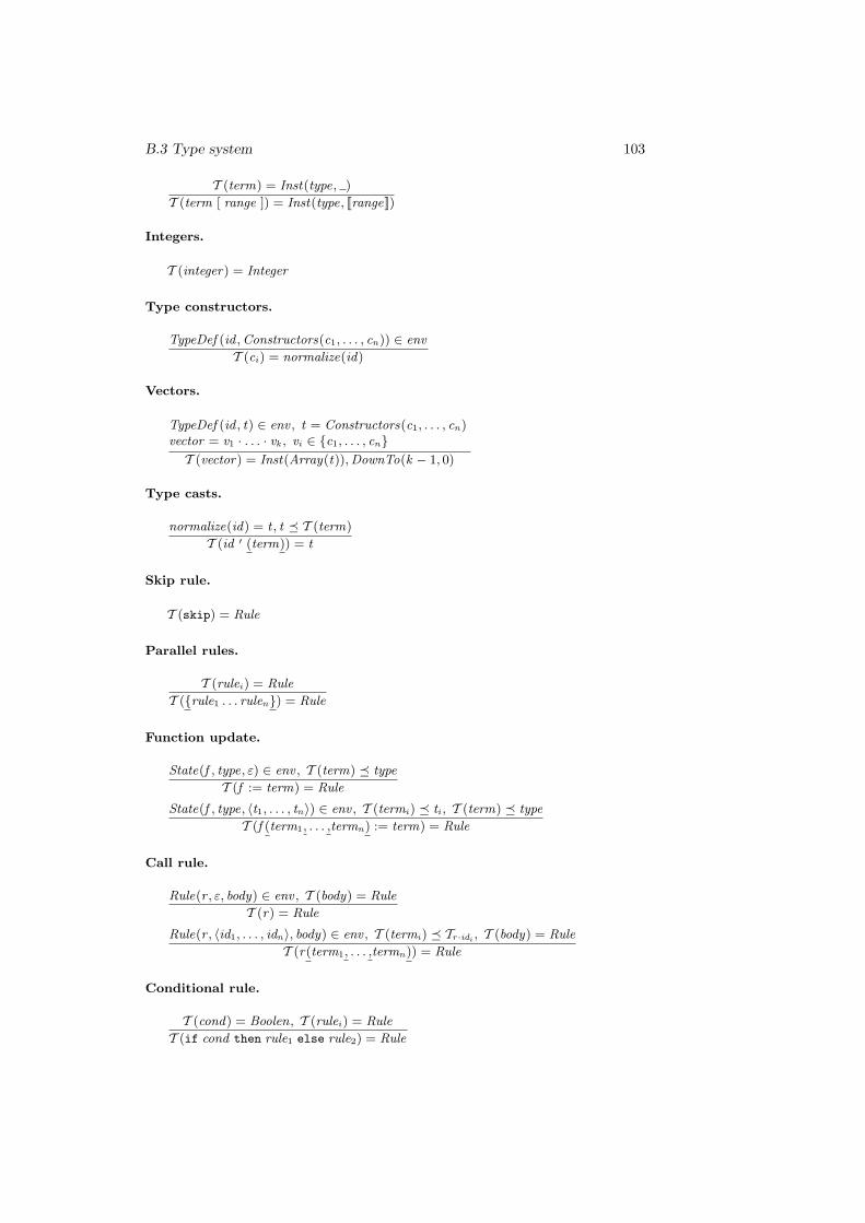
B.3 Type system 103

T (term) = Inst(type, )

T (term [ range ]) = Inst(type, [[range]])

Integers.

T (integer) = Integer

Type constructors.

TypeDef (id ,Constructors(c1, . . . , cn)) ∈ env

T (ci) = normalize(id)

Vectors.

TypeDef (id , t) ∈ env , t = Constructors(c1, . . . , cn)vector = v1 · . . . · vk , vi ∈ {c1, . . . , cn}T (vector) = Inst(Array(t)),DownTo(k − 1, 0)

Type casts.

normalize(id) = t , t � T (term)

T (id ′ (term)) = t

Skip rule.

T (skip) = Rule

Parallel rules.

T (rulei) = Rule

T ({rule1 . . . rulen}) = Rule

Function update.

State(f , type, ε) ∈ env , T (term) � type

T (f := term) = Rule

State(f , type, 〈t1, . . . , tn〉) ∈ env , T (termi) � ti , T (term) � type

T (f (term1, . . . ,termn) := term) = Rule

Call rule.

Rule(r , ε, body) ∈ env , T (body) = Rule

T (r) = Rule

Rule(r , 〈id1, . . . , idn〉, body) ∈ env , T (termi) � Tr·idi , T (body) = Rule

T (r(term1, . . . ,termn)) = Rule

Conditional rule.

T (cond) = Boolen, T (rulei) = Rule

T (if cond then rule1 else rule2) = Rule


B.4 Constraints

Constraints for C = [component id uses decl1 . . . decln end component]

Main rule. The component contains a rule having the same name as the component:

∃ Rule(id , ε, body) ∈ env : T (id) = Rule

Outputs. For each output id1, there is either a nullary function with the same name,or id1 is connected to an output id2. The corresponding types must be compatible.

∀ Out(id1, type) ∈ env : ∃Fun(id1, ε, body) ∈ env : T (id1) � type ∨∃OutOut(id1, id2) ∈ env : T (id2) � type

Type compatibility of connections.

∀ OutOut(id1, id2) ∈ env : T (id2) � T (id1)∀ InOut(id1, id2) ∈ env : T (id2) � T (id1)∀ InIn(id1, id2) ∈ env : T (id2) � T (id1)∀ InFun(id1, id2) ∈ env : T (id2) � T (id1)

References

[1] J. R. Abrial. The B-Book. Assigning Programs to Meanings. CambridgeUniversity Press, 1996.

[2] M. Anlauff. XASM – An extensible, component-based Abstract State Ma-chines language. In Gurevich et al. [36], pages 69–90.

[3] M. Anlauff, D. Fischer, P. W. Kutter, J. Teich, and R. Weper. Hierarchi-cal microprocessor design using XASM. In Moreno-Dıaz and Quesanda-Arencibia [52], pages 271–274. Extended Abstract.

[4] H. Barendregt. The Lambda Calculus. Its Syntax and Semantics, vol-ume 103 of Studies in Logic and the Foundations of Mathematics. North-Holland, 1981.

[5] S. Berezin, S. Campos, and E. M. Clarke. Compositional reasoning inmodel checking. In W.-P. de Roever, H. Langmaack, and A. Pnueli, editors,Compositionality. The Significant Difference, volume 1536 of Lecture Notesin Computer Science, pages 81–102. Springer-Verlag, 1998.

[6] J. Berge, O. Levia, and J. Rouillard. Hardware Component Modeling.Kluwer Academic Publishers, 1996.

[7] R. Bird. Introduction to Functional Programming using Haskell. PrenticeHall, 1998.

[8] C. Bohm and G. Jacopini. Flow diagrams, Turing Machines, and languageswith only two formation rules. Communications of the ACM, 9(5):366–371,1966.

[9] E. Borger. Why use evolving algebras for hardware and software engineer-ing? In M. Bartosek, J. Staudek, and J. Wiederman, editors, Proceedingsof SOFSEM’95, 22nd Seminar on Current Trends in Theory and Practiceof Informatics, volume 1012 of Lecture Notes in Computer Science, pages236–271. Springer-Verlag, 1995.

[10] E. Borger. High level system design and analysis using Abstract StateMachines. In D. Hutter, W. Stephan, P. Traverso, and M. Ullmann, editors,Current Trends in Applied Formal Methods (FM-Trends 98), number 1641in Lecture Notes in Computer Science, pages 1–43. Springer-Verlag, 1999.

[11] E. Borger, A. Cavarra, and E. Riccobene. An ASM semantics for UMLActivity Diagrams. In T. Rust, editor, Algebraic Methology and Software

105

106 REFERENCES

Technology, number 1816 in Lecture Notes in Computer Science. Springer-Verlag, 2000.

[12] E. Borger, A. Cavarra, and E. Riccobene. Modeling the dynamics of UMLstate machines. In Gurevich et al. [36], pages 223–241.

[13] E. Borger, U. Glasser, and W. Muller. Formal definition of an abstractVHDL’93 simulator by EA-Machines. In C. D. Kloos and P. T. Breuer,editors, Formal Semantics for VHDL, pages 107–139. Kluwer AcademicPublishers, 1995.

[14] E. Borger, E. Gradel, and Y. Gurevich. The Classical Decision Problem.Perspectives in Mathematical Logic. Springer-Verlag, 1997.

[15] E. Borger, B. Horger, D. L. Parnas, and D. Rombach, editors. RequirementsCapture, Documentation and Validation, Dagstuhl-Seminar-Report 242,1999. Web pages at http://www.iese.fhg.de/Dagstuhl/seminar99241.html.

[16] E. Borger and J. Huggins. Abstract State Machines 1988–1998. CommentedASM bibliography. Bulletin of EATCS, 64:105–127, February 1998. Up-dated bibliography available at http://www.eecs.umich.edu/gasm/.

[17] E. Borger, P. Pappinghaus, and J. Schmid. Report on a practical applica-tion of ASMs in software design. In Gurevich et al. [36], pages 361–366.Online available at http://www.tydo.de/files/papers/.

[18] E. Borger, E. Riccobene, and J. Schmid. Capturing requirements by Ab-stract State Machines. the Light Control case study. Journal of UniversalComputer Science, 6(7), 2000.

[19] E. Borger and J. Schmid. Composition and submachine concepts. In P. G.Clote and H. Schwichtenberg, editors, Computer Science Logic (CSL 2000),number 1862 in Lecture Notes in Computer Science, pages 41–60. Springer-Verlag, 2000.

[20] E. Borger and W. Schulte. Modular design for the Java Virtual Machine ar-chitecture. In E. Borger, editor, Architecture Design and Validation Meth-ods, pages 297–357. Springer-Verlag, 2000.

[21] W. Brauer. Automatentheorie. B. G. Teubner, 1984.

[22] A. Bruggemann, L. Priese, D. Rodding, and R. Schatz. Modular decompo-sition of automata. In E. Borger, G. Hasenjager, and D. Rodding, editors,Logic and Machines. Decision Problems and Complexity, number 171 inLecture Notes in Computer Science, pages 198–236. Springer-Verlag, 1984.

[23] A. Cavarra and E. Riccobene. Simulating UML statecharts. In Moreno-Dıaz and Quesanda-Arencibia [52], pages 224–227. Extended Abstract.

[24] K. C. Chang. Digitial Design and Modeling with VHDL and Synthesis.IEEE Computer Society Press, 1997.

[25] K. Chen and M. Odersky. A type system for a lambda calculus with assign-ment. In Theoretical Aspects of Computer Science, number 789 in LectureNotes in Computer Science, pages 347–364. Springer-Verlag, 1994.

http://www.eecs.umich.edu/gasm/

http://www.tydo.de/files/papers/

REFERENCES 107

[26] E. M. Clarke, O. Grumberg, and D. E. Long. Model checking and abstrac-tion. ACM Transactions on Programming Languages and Systems, pages343–354, 1992.

[27] E. M. Clarke, O. Grumberg, and D. E. Long. Model checking and ab-straction. ACM Transactions on Programming Languages and Systems,16(5):1512–1542, 1994.

[28] M. Davis. The Universal Computer. The Road from Leibniz to Turing.W.W. Norton, New York, 2000.

[29] G. Del Castillo. The ASM Workbench. an open and extensible tool envi-ronment for Abstract State Machines. In Proceedings of the 28th AnnualConference of the German Society of Computer Science. Technical Report,Magdeburg University, 1998.

[30] G. Del Castillo. The ASM-Workbench. A tool environment for computeraided analysis and validation of ASM models. PhD thesis, University ofPaderborn, 2000.

[31] A. Dold. A formal representation of Abstract State Machines using PVS.Verifix Report Ulm/6.2, 1998.

[32] O. Grumberg and D. E. Long. Model checking and modular verification.ACM Transactions on Programming Languages and Systems, 16(3):843–871, 1994.

[33] Y. Gurevich. Evolving Algebras 1993. Lipari Guide. In E. Borger, editor,Specification and Validation Methods, pages 9–36. Oxford University Press,1995.

[34] Y. Gurevich. May 1997 draft of the ASM guide. Technical Report CSE-TR-336-97, University of Michigan EECS Department, 1997.

[35] Y. Gurevich. Sequential Abstract State Machines capture sequential algo-rithms. ACM Transactions on Computational Logic, 1(1), 2000.

[36] Y. Gurevich, M. Odersky, and L. Thiele, editors. Abstract State Machines,ASM 2000, number 1912 in Lecture Notes in Computer Science. Springer-Verlag, 2000.

[37] Y. Gurevich and M. Spielmann. Recursive Abstract State Machines. Jour-nal of Universal Computer Science, 3(4):233–246, 1997.

[38] C. Hall, K. Hammond, S. P. Jones, and P. Wadler. Type classes in Haskell.ACM Transactions on Programming Languages and Systems, 18(2):109–138, 1996.

[39] U. Heinkel. VHDL reference. A pratical guide to computer-aided integratedcircuit design, including VHDL-ASM. John Wiley Ltd, 2000.

[40] T. A. Henzinger, S. Qadeer, S. K. Rajamani, and S. Tasıran. An assume-guarantee rule for checking simulation. Formal Methods in Computer-AidedDesign, 1997.

108 REFERENCES

[41] G. Hutton and E. Meijer. Monadic parser combinators. Technical Re-port NOTTCS-TR-96-4, Department of Computer Science, University ofNottingham, 1996.

[42] M. P. Jones. An introduction to Gofer, 1991. Available in the Goferdistribution at http://www.cse.ogi.edu/~mpj/goferarc/index.html.

[43] M. P. Jones. Gofer. Functional programming environment, 1994. Web pageat http://www.cse.ogi.edu/~mpj/goferarc/index.html.

[44] M. P. Jones. The implementation of the Gofer functional programmingsystem. Research Report YALEU/DCS/RR-1030, 1994.

[45] S. P. Jones and P. Wadler. Imperative functional programming. In Confer-ence record of the 20th Annual ACM SIGPLAN-SIGACT Symposium onPrinciples of Programming Languages, Charleston, South Carolina, pages71–84, 1993.

[46] S. C. Kleene. Introduction to Metamathematics. D. van Nostrand, Prince-ton, New Jersey, 1952.

[47] J. Launchbury. A natural semantics for lazy evaluation. In ConferenceRecord of the 20th Annual ACM SIGPLAN-SIGACT Symposium on Prin-ciples of Programming Languages, pages 144–154, 1993.

[48] L. Lavagno and A. Sangiovanni-Vincentelli. Algorithms for Synthesis andTesting of Asynchronous Circuits. Kluwer Academic Publishers, 1993.

[49] S. Liang, P. Hudak, and M. Jones. Monad transformers and modular inter-preters. In Conference record of POPL ’95, 22nd ACM SIGPLAN-SIGACTSymposium on Principles of Programming Languages, pages 333–343, 1995.

[50] N. A. Lynch and M. R. Tuttle. An introduction to input/output automata.Technical Report MIT/LCS/TM-373, M.I.T. Laboratory for Computer Sci-ence, 1988.

[51] J. Maraist, M. Odersky, and P. Wadler. The call-by-need lambda calculus.Journal of Functional Programming, 8(3), 1994.

[52] R. Moreno-Dıaz and A. Quesanda-Arencibia, editors. Formal Methods andTools for Computer Science, Eurocast. Universidad de Las Palmas de GranCanaria, 2001.

[53] M. Odersky. How to make destructive updates less destructive. In Pro-ceedings, 18th ACM Symposium on Principles of Programming Languages,pages 25–26, 1991.

[54] M. Odersky. Programming with variable functions. ICFP’98, Proceedingsof the 3rd ACM SIGPLAN International Conference on Functional Pro-gramming, 34(1):105–116, 1998.

[55] M. Odersky, D. Rabin, and P. Hudak. Call-by-name, assignment, andthe lambda calculus. In Conference record of the 20th Annual ACMSIGPLAN-SIGACT Symposium on Principles of Programming Languages,Charleston, South Carolina, pages 43–56, 1993.

http://www.cse.ogi.edu/~mpj/goferarc/index.html

http://www.cse.ogi.edu/~mpj/goferarc/index.html

REFERENCES 109

[56] D. L. Parnas. Information distribution aspects of design methodology. InInformation Processing 71, pages 339–344. North Holland Publishing Com-pany, 1972.

[57] L. C. Paulson. ML for the Working Programmer. Cambridge UniversityPress, 1996.

[58] A. Pnuelli. In transition from global to modular temporal reasoning aboutprograms. In K. R. Apt, editor, Logics and Models of Concurrent Systems,Computer and System Science, pages 123–144. Springer-Verlag, 1985.

[59] G. Schellhorn. Verifikation abstrakter Zustandsmaschinen. PhD thesis, Uni-versity of Ulm, 1999. For an english version see http://www.informatik.uni-ulm.de/pm/kiv/papers/verif-asms-english.pdf.

[60] J. Schmid. Executing ASM specifications with AsmGofer. Web pages athttp://www.tydo.de/AsmGofer/, 1999.

[61] J. Schmid. Compiling Abstract State Machines to C++. In Moreno-Dıazand Quesanda-Arencibia [52], pages 298–300. Extended Abstract.

[62] N. Shankar. Lazy compositional verification. In H. Langmaack, A. Pnueli,and W.-P. de Roever, editors, Compositionality. The Significant Differ-ence, volume 1536 of Lecture Notes in Computer Science, pages 541–564.Springer-Verlag, 1998.

[63] R. F. Stark and J. Schmid. Java bytecode verification is not possible.In Moreno-Dıaz and Quesanda-Arencibia [52], pages 232–234. ExtendedAbstract.

[64] R. F. Stark, J. Schmid, and E. Borger. Java and the Java Virtual Machine.Definition, Verification, Validation. Springer-Verlag, 2001. See web pagesat http://www.inf.ethz.ch/~jbook/.

[65] E. D. Thomas and R. P. Moorby. The Verilog Hardware Description Lan-guage. Kluwer Academic Publishers, 2000.

[66] S. Thompson. Haskell. The Craft of Functional Programming. Addison-Wesley, second edition, 1999.

[67] T. Vullinghs, W. Schulte, and T. Schwinn. An introduction to Tk-Gofer, 1996. Web pages at http://pllab.kaist.ac.kr/seminar/haha/tkgofer2.0-html/user.html.

[68] P. Wadler. The essence of functional programming. In Proceedings ofthe 19th Symposium on Principles of Programming Languages, pages 1–14,1992.

[69] P. Wadler. Monads for functional programming. In J. Jeuring and E. Mei-jer, editors, 1st International Spring School on Advanced Functional Pro-gramming Techniques, pages 24–52. Springer-Verlag, 1995.

[70] J. Walton. Conway’s Game of Life, 2000. Web pages at http://www.reed.edu/~jwalton/.

http://www.informatik.uni-ulm.de/pm/kiv/papers/verif-asms-english.pdf

http://www.informatik.uni-ulm.de/pm/kiv/papers/verif-asms-english.pdf

http://www.tydo.de/AsmGofer/

http://www.inf.ethz.ch/~jbook/

http://pllab.kaist.ac.kr/seminar/haha/tkgofer2.0-html/user.html

http://pllab.kaist.ac.kr/seminar/haha/tkgofer2.0-html/user.html

http://www.reed.edu/~jwalton/

http://www.reed.edu/~jwalton/

110 REFERENCES

[71] A. Wikstrom. Functional programming using Standard ML. Prentice Hall,1987.

[72] K. Winter. Model checking for Abstract State Machines. Journal of Uni-versal Computer Science, 3(5):689–701, 1997.

[73] Q. Xu and M. Swarup. Compositional reasoning using the assumption-commitment paradigm. In W.-P. de Roever, H. Langmaack, and A. Pnueli,editors, Compositionality. The Significant Difference, volume 1536 of Lec-ture Notes in Computer Science, pages 565–583. Springer-Verlag, 1998.

[74] A. Zamulin. Object-oriented Abstract State Machines. In Proceedings ofthe 28th Annual Conference of the German Society of Computer Science.Technical Report, Magdeburg University, 1998.

implementation and refinement techniques for abstract

Documents