Louisiana State UniversityLSU Digital Commons

LSU Master's Theses Graduate School

2007

Impingement Heat Transfer In The Leading EdgeCavity Of A Gas Turbine VaneAmar Jeetendra Panchangam NivarthiLouisiana State University and Agricultural and Mechanical College

Follow this and additional works at: https://digitalcommons.lsu.edu/gradschool_theses

Part of the Accounting Commons

This Thesis is brought to you for free and open access by the Graduate School at LSU Digital Commons. It has been accepted for inclusion in LSUMaster's Theses by an authorized graduate school editor of LSU Digital Commons. For more information, please contact gradetd@lsu.edu.

Recommended CitationPanchangam Nivarthi, Amar Jeetendra, "Impingement Heat Transfer In The Leading Edge Cavity Of A Gas Turbine Vane" (2007).LSU Master's Theses. 263.https://digitalcommons.lsu.edu/gradschool_theses/263

IMPINGEMENT HEAT TRANSFER IN THE LEADING EDGE CAVITY OF A GAS TURBINE VANE

Submitted to the Graduate Faculty of the Louisiana State University and

Agricultural and Mechanical College in partial fulfillment of the

requirements for the degree of Master of Science in Mechanical Engineering

in

The Department of Mechanical Engineering

by Amar Jeetendra Panchangam Nivarthi

B.S., Osmania University, Hyderabad, India, 2004 May 2008

ii

Acknowledgements

First of all I would like to express my sincere gratitude to Dr. Shengmin Guo and

Dr. Sumanta Acharya for providing me with an opportunity to work in this research.

Without their guidance, financial support and help, this work would never have been

completed. I’d like to thank them for their belief and faith in me.

I am indebted to my project liaisons Dr. Mike Blair and Dr. Jesse Christophel of

Pratt and Whitney for their continued support of this project both financially and

technically. I would also like to thank my committee member Dr. Muhammad Wahab for

his valuable suggestions

Last, but not the least, I would like to thank my friends and family for their

motivation, support and help.

iii

Table of Contents

Acknowledgements ....................................................................................................................... ii

Abstract ......................................................................................................................................... iv

Chapter 1: Introduction ................................................................................................................1 1.1 Impingement Cooling .....................................................................................................3 1.2 Literature Survey ............................................................................................................5 1.3 Objectives and Outline of the Thesis .............................................................................9

Chapter 2: Discharge Coefficients of Film Cooling Holes and Impingement Holes..............11 2.1 Experimental Setup ......................................................................................................11 2.1.1 Test Section and Flow Layout .......................................................................11 2.1.2 Impingement Plate .........................................................................................12 2.1.3 Target Surface ................................................................................................12 2.1.4 Coolant Supply ...............................................................................................13 2.2 Flow Calculations- Coefficient of Discharge ..............................................................15 2.2.1 Procedure for Impingement Hole Cd Measurement ..................................16 2.2.2 Procedure for Film Cooling Hole Cd Measurement ...................................18

Chapter 3: Liquid Crystal Based Heat Transfer Tests ............................................................22 3.1 Experimental Setup ......................................................................................................22 3.1.1 Temperature Measurement ..........................................................................22 3.1.2 Heating Arrangement ....................................................................................22 3.1.3 CCD-Camera and Endoscope .......................................................................23 3.2 Thermochromic Liquid Crystal Technique ...............................................................23 3.3 Benchmarking of the Camera-Endoscope Combination ...........................................25 3.3.1 Experimental Procedure and Results ...........................................................27 3.4 Theory and Mathematical Formulation .....................................................................31 3.5 Experimental Procedure ..............................................................................................34 3.6 Post Processing of Liquid Crystal Images ..................................................................35

Chapter 4: Heat Transfer Results and Discussion ....................................................................39 4.1 Heat Transfer Results ...................................................................................................39 4.1.1 Heat Transfer Contours ................................................................................40 4.1.2 Area Average of Heat Transfer Coefficients ..............................................51 4.2 Discussion of the Results ..............................................................................................57 4.2.1 Jet Impingement on Inclined Surface ..........................................................58 4.2.2 Cross Flow Momentum versus Jet Momentum ..........................................61 4.2.3. Film Cooling Configuration .........................................................................64 4.2.4. Flow Path of Least Resistance .....................................................................66

Chapter 5: Conclusions ...............................................................................................................67

References .....................................................................................................................................68

Vita ................................................................................................................................................71

iv

Abstract

Jet Impingement Cooling is an internal cooling technique used in the leading edge

cavities of Turbine Vanes. This involves a series of jets impinging onto the internal

surfaces of a turbine vane/blade through the impingement plate. For the model tested

here, the area around the blade/vane leading edge was studied for both heat transfer

performance and aerodynamics losses. The performance of an Impingement cooling

system depends on parameters like the spent flow effect on the downstream jet, film

cooling configuration, and tip flow condition. The present study focuses on analyzing the

effect of these parameters on a unique impingement cooling configuration. A Liquid

Crystal based technique was used to obtain the heat transfer distribution on the target

surface. A novel Camera-Endoscope combination was used to capture the liquid crystal

images in a confined space. Heat Transfer Contours were obtained for a total of six

different cases based on differing film cooling hole configurations and tip condition. Peak

heat transfer values are observed in the impingement zone along with a characteristic

reduction in heat transfer as we move away from the impingement zone. The results

indicated that the cross flow had a negative impact on the peak heat transfer value but

improved the uniformity of heat transfer distribution. The film cooling configuration was

found to affect the amount of cross flow and the location of the impingement zone of the

jet. The cross flow effect is found to have reduced effect with an increase in the available

number of film cooling holes leading to an increase in the peak heat transfer. The tip

condition was altered for the last case in which it adversely affected the extent of jet

impingement. Line plots for all the contours showed the spent flow effect. A fluid

dynamic analysis of all the above effects was presented.

1

Chapter 1

Introduction

The gas turbine is extensively used as a power plant for aircraft propulsion and power

generation. The main components of a gas turbine are the compressor, combustion

chamber and the turbine. A schematic of all the stages is shown in Fig 1.1(i). The

schematic can be represented by a closed thermodynamic cycle shown in Fig 1.1(ii). The

cycle has four stages, representing the physical phenomena taking place at different

sections of a gas turbine at the same time. The fresh air enters the compressor (1-2) where

it undergoes a compression. The typical compressor efficiency is around 85% to 88% for

a modern design. However, for simplicity, an isentropic compression was used here.

Subsequently the compressed air flows into the combustion chamber where it mixes with

the fuel and is ignited resulting in energy addition (2-3) to the flow. In this process, the

small pressure loss is mainly due to flow mixing and the viscous effect, thus a constant

pressure process was used here. The hot gas mixture of air and combustion products then

enters the turbine where it expands to the low back pressure (3-4) and produces power.

The irreversibility loss in the expansion is small thus an isentropic process can be used in

the first approximation. A part of this power is used to drive the compressor and the rest

is extracted from the system as either thrust (jet engine) or shaft work (power

production). As with any internal combustion engine the main aim is to achieve better

performance and reliability. The demand for fuel efficient and higher thrust engines has

posed a huge challenge to the engineers. Both thermal efficiency and thrust output

increase with increasing Turbine Inlet Temperature. This dependence illustrated in the

Fig 1.2 below.

2

4

3

2

1

0

250

500

750

1000

1250

1500

1750

2000

0 500 1000 1500 2000

Specific Entropy, s [J/kg K]

Tem

pera

ture

, T [K

]

r T =6, r p =10

(i) (ii)

Fig 1.1: Gas Turbine Schematic and thermodynamic cycle [1]

Fig 1.2: Increase in Specific Core Power with Increasing Inlet Temperature (Saunter et al., 1992 )

The limiting factor to increasing turbine inlet temperature is the permissible

operating temperature of the blade material. Therefore cooling of the blades is the only

way to use the existing blade material with increased inlet temperatures. The modern gas

3

turbine blades have both internal as well surface cooling mechanisms which utilize the air

extracted from the compressor. Cooling is crucial to safeguard the engine for normal

operation, also the cooling leads to a reduced thermal efficiency, an optimized cooling

technique has to be developed.

Figure 1.3 shows the schematic of a blade cooling system that is both internally

and externally cooled. As mentioned above, the compressor provides the coolant air to

the cooling passages. The coolant passes from the trailing edge, where a pin fin system is

used to maximize heat transfer, through the internal cooling passages and rib turbulators

into the leading edge. The leading edge region has a plate with a number of holes which

provides a jet impingement cooling mechanism on the inner surface of the cavity. The

coolant is then ejected through a row of holes on the leading edge itself known as the film

cooling holes. The exiting air acts as a protective film between the outer surface of the

leading edge and the incoming hot mainstream air.

1.1 Impingement Cooling

Jet impingement heat transfer is one of the most effective heat transfer

enhancement techniques in the internal cooling of gas turbine vanes. This involves the

impingement of a fluid jet on the internal surface of the leading edge of a vane/blade to

provide an extremely high rate of cooling. The heat transfer distribution around a turbine

vane is shown in Fig 1.4. Jet impingement heat transfer is suitable for the leading edge of

a vane, where the thermal load is highest and a thicker cross-section enables

accommodation of a coolant plenum and impingement holes. Jet impingement cooling is

capable of providing an extremely high peak heat transfer coefficient for the region under

4

the impingement jet. The mechanism of heat transfer of a jet impinging a target surface is

illustrated in Fig 1.5

Fig 1.3: Schematic of a cooling system in a Modern Multi-Pass Turbine Blade (Han, Dutta and Ekkad, 2000)

The jet after impinging spreads along the target surface providing a thin stagnant

boundary layer. A stagnant core is formed at the point where the jet impinges. The

coolant in the stagnant core is continuously replaced by the jet thus providing a step

change in temperature at any given point in time. This creates an extremely high peak in

the heat transfer. As the coolant fluid moves away from the core, heat transfer takes place

in the convection mode at a comparatively lesser rate. A typical heat transfer distribution

in a jet impingement system is shown in Fig 1.6. As evident from Fig 1.6, although the jet

5

Fig 1.4: Variation of heat transfer rate around a turbine vane (Han, Dutta and Ekkad, 2000)

impingement cooling has the advantage of achieving significantly enhanced overall heat

transfer rates it inherently suffers from a highly non uniform cooling distribution.

Therefore a number of jets are used in tandem to provide a more uniform heat

transfer distribution. This gives rise to design concerns such as the effect of spent flow

from the upstream jets on the downstream jets and interference between impingement

flows of adjacent jets. Designers have to therefore employ a host of geometric parameters

like the hole geometry, shape & size and spacing of the holes to optimize the heat transfer

distribution. Also other parameters like to jet to cross flow ratio and positioning of the

jets with respect to film cooling holes have to be considered in the design process.

1.2 Literature Survey

Research results during the past four decades on jet impingement heat transfer are

Possibility of shock - boundary layer interaction if severe it can cause separation

UNSTEADY WAKE FLOW

Possibility of -transition followed by relaminarisation

Possibility of Goertler instabilities. due to concave curvature

6

available in a large body of literature. Livingood and Hrycak, 1973, Martin, 1977, Downs

and James, 1987, and Humber and Viskanta, 1994, have provided extensive reviews of

Fig 1.5: Illustration of Jet Impingement and Flow visualization photograph (http://www.me.umn.edu)

Fig 1.6: Heat Transfer Distribution in a Jet Impingement System (Bruchez and Goldstein, 1975)

previous literature. Both analytical and numerical studies were performed. Early research

showed that the predominant factor in jet impingement heat transfer is the effect of the

spent flow. Goldstein and Timmers, 1982, showed that spent air from upstream jets

tended to lower local heat transfer coefficients and, in the limit, a flow visualization

7

showed that the cross flow can sweep away the downstream jets such that the jet

impingement was prevented. A series of studies of jet impingements heat transfer under

the effect of imposed (external) cross flow in addition to the existing spent flow were

conducted. Florschuetz et. al., 1980, 1981, 1984, and Florschuetz, 1982, found that

increasing the ratio between the imposed cross-flow mass flow rate and impingement jet

flow rate from 0.2 to 0.4 could significantly reduce Nusselts number by a factor greater

than 2.5.

Bruchez and Goldstein, 1975, experimentally studied the influence of cross flow

on the heat transfer characteristic of partially confined and staggered impinging jets

issuing from discrete round holes and slots respectively. For single or multiple jets, flow

visualization results showed that the cross flow made the flow highly three-dimensional,

which also increased the complexity of the flow structure and heat transfer situation.

Huang et al., 1998, presented detailed heat transfer distributions for an array of in-line

jets impinging on a plate with different cross flow orientations by employing a transient

liquid crystal method. The different cross flow directions were created by changing the

test section open ends. They reported that the highest heat transfer coefficients are

obtained for a cross flow orientation where flow exits in both directions.

For the imposed cross flow case, Huang, Mujumdar, and Douglas, 1984

conducted a numerical investigation on the effect of the cross flow rate on the heat

transfer performance under a turbulent impinging slot jet. They compared the predicted

Nusselts number distribution including the effect of cross flow with those without cross

flow. It was found that the location of the maximum Nusselts number shifted downstream

due to the deflection of the jet by the cross flow. They further observed that the Nusselts

8

number far downstream from the slot exit for the case with imposed cross flow was

higher than that without cross flow, which was in agreement with the Metzger, et al.'s,

1969 experimental observation on round jets in an imposed cross flow. The decrease of

the Nusselts number over the downstream region was due to the total mass flow rate

exhausted through downstream direction which increased as the cross-flow rate was

increased. Galant and Martinez, 1982, presented a formulation of the cross flow influence

upon impingement heat transfer rates for arrays of circular based on the jet height and

diameter. The formulation is shown below where Z=Height of the jet, D=Diameter of

the jet, m= Cross flow to jet momentum ratio and ψ =Analytical Function of Z/D

xxNu

mDZm

DZ

Re08.0

067.0, 951.0536.0

=

⎟⎠⎞

⎜⎝⎛=⎟

⎠⎞

⎜⎝⎛ −

−

ψ

A study more relevant to the current situation was presented by Taslim and

Setayeshgar, 2001, through a series of experiments of jet impingement on a leading edge

wall with film holes. They studied circular and racetrack shaped impingement holes

under both pure shower head and simulated tip flow condition. The jets in this study had

a greater height (Z/D) than the jets used in the current study. Fig 1.7 shows the Nusselts

number variation with respect to Jet Reynolds number for different flow configurations.

The 70 % showerhead case in Fig.1.7 refers to the flow configuration where 30 %

of the flow exits through the tip while the rest exits through the film cooling holes. The

current study is being conducted to obtain the heat transfer characteristics of a jet

impingement system on a unique target surface geometry under different cross flow

conditions and film cooling configurations.

Eq. 1.1

9

1.3 Objectives and Outline of the Thesis

The current study involved a total of three stages. They are:

Task 1: Calculation of Coefficient of Discharge of the Impingement and the Film

Cooling Holes (Chapter 2)

Fig 1.7: Comparison of results of racetrack shaped and round cross over jets (Taslim and Setayeshgar, 2001 )

Task 2: Benchmarking of the Camera-Endoscope technique against a Standard Camera-

Lens Technique (Chapter 2)

Task 3: Liquid crystal based heat transfer tests on the internal cooling cavity surfaces

under different impingement and cross flow conditions (Chapter 3)

The purpose of the first task is to obtain more information on the flow distribution

within the test section under the given flow conditions. The discharge coefficient values

are to be supplied to the Project Sponsor for the development of a flow model. The

second task involved validation the novel image capturing technique being used in the

current study by comparing it with a proven camera-lens technique. Heat transfer tests

10

were carried out on a rectangular channel using both the techniques and the results were

compared. The third task involved obtaining the heat transfer contours for jet

impingement under various configurations. The objective of these tests is to gain an

understanding of the effect of different test parameters i.e. amount of cross flow, film

cooling configuration and tip flow condition on the final heat transfer contour. The term

cross flow in the present case refers to the existing spent flow from the upstream jets as

well as an external cross flow provided in the radial direction. Each case had a different

combination of the film cooling holes and hence there was a variation in the number of

film holes available in each case. A variation of one of these cases was performed with a

closed tip condition to obtain an understanding of the effect of tip condition on the heat

transfer.

11

Chapter 2

Discharge Coefficients of Film Cooling Holes and Impingement Holes

2.1 Experimental Setup

The following sub sections describe the experimental set-up used in calculating

the discharge coefficients.

2.1.1 Test Section and Flow Layout

The coolant flow from the supply tank is routed through a ball valve and a

particulate filter to the flow circuit shown in Fig.2.1. The flow circuit consists of two

branches: one leading to the impingement array and the other branch feeds the external

cross flow plenum. At the inlet of each branch a Needle valve (Valve 2 and Valve 3 in

Fig 2.1) is installed to adjust the flow rates in the respective branches. By adjusting these

two valves, the flow rate through the test section can be conveniently controlled.

Fig 2.1: Flow Circuit to that supplies air to the impingement plenum and the cross flow plenum

The Flow rates in the branches are monitored by two Omega FLR-D series, digital

flow meters. The operating pressure is 100 psi and the operating range is 20 CFM-250

CFM. The air pressure at the inlet of these flow meters is obtained from an upstream

pressure gauge and the flow is corrected for that value of the pressure.

12

The test section, in which the target plate and the impingement plate are housed,

is made of perspex. It consists of the impingement plenum, peanut cavity and the outer

chamber into which the peanut cavity discharges its flow. Figure 2.2 shows the cross

section of the test section. The relevant chambers are labeled. The peanut cavity is

encompassed by the target surface, the impingement plate and the support plate. The

peanut cavity represents a scaled up model of the leading edge cavity of a turbine vane.

The impingement cavity is made up of the impingement plate, the support plate and the

external structure. The feed air from the air storage tank enters the impingement chamber

and flows through the impingement holes into the peanut cavity where it strikes the target

surface. The air from the peanut cavity sits through the film cooling holes into the

external chamber which in turn exhausts the air into the atmosphere through two 2-inch

holes. Figure 2.3 shows the solid model of the test section. The arrow in the figure

indicates the cross flow direction. The tip exit of the peanut cavity is at the end pointed

by the arrow. The target surface and impingement plate are described in detail in the sub

sections.

2.1.2 Impingement Plate

The impingement plate is also constructed from Perspex. It has an inline row

impingement holes. There are total of three sets of impingement holes with varying

diameter. All the three sets and their arrangement are shown in Fig 2.4

2.1.3 Target Surface

The target surface is shown in Fig 2.5. It is constructed from Perspex and

represents a section of the leading edge of a turbine vane. It has five rows of inclined film

cooling holes of which the first four (Rows 1-4) represent the showerhead rows and fifth

13

Pressure Tap 1- Used to measure static pressure within the chamber

Pressure Tap 2- used to measure the stagnation pressure of theair stream upstream of the hole.

Air Supply

2 inches

Peanut Cavity

Impingement Chamber

row (row 5) represents the gill row. The impingement jets strike the target on inclined

surface on which the row 4 is located. This represents the suction side of the leading edge

cavity in a turbine vane. As evident from the geometry, the jet strikes the target surface at

an angle of 30.50. The relevant dimensions are shown in the Fig. 3.6. A layer of black

paint is sprayed on the inside of the target surface. Liquid crystal is then applied in the

form of a fine spray on the black paint.

Fig 2.2: Cross Sectional view of the Test Section

2.1.4 Coolant Supply

The feed air to the impingement plate comes from a dedicated Atlas Copco GR

110 two-stage screw compressor. The air from the compressor is passed through a

Pneumatech Inc. heatless, regenerative air dryer to remove any moisture that might be

present in the supply. The pressurized, dry air from the drier is stored in a storage tank

downstream. The purpose of the storage tank is to ensure a constant supply of dry air

Target Surface

External Chamber

Impingement Plate

Support Plate

14

without transmitting any supply pressure fluctuations due to the compressor cycle of

operation.

Fig 2.3: Solid Model of the Test Section

Fig 2.4: Impingement Plate and arrangement of the Impingement Holes

15

Fig 2.5: Target Surface

2.2 Flow Calculations- Coefficient of Discharge

The first stage of the project involved the measurements of the discharge coefficients

of the Impingement Holes and Film Cooling Holes. This stage of the project was

specifically carried out on the request of the sponsor in order for them to set up a flow

model of the test rig based on the Discharge Coefficients furnished by the team at LSU.

The flow model was computed using in-house software at Pratt and Whitney. The input

parameters to this flow model were the pressure ratios across the impingement plate and

the target plate along with the discharge coefficients of the holes. These parameters were

used to set up a network flow model based on the principle of conservation of flow across

all the sets of holes to compute the flow distribution across the Impingement plate and the

16

target surface. The sponsor then used the consequent flow distribution model as the basis

to estimate the heat transfer coefficient distribution at the test location.

2.2.1 Procedure for Impingement Hole Cd Measurement

The discharge coefficients for the impingement holes are calculated by opening up

the peanut cavity. This is achieved by removing the target surface from the top of the

impingement plate and allowing the air to pass through the impingement holes into the

outer plenum instead of the impingement cavity. A static pressure probe is then used to

measure the pressure in the impingement plenum upstream of the impingement holes and

the downstream pressure at the ‘vena contracta’ (cross section where the jet has the least

diameter) of the jet. In case of the impingement holes, which have a contoured edge, the

vena contracta is located exactly at the exit of the hole. These values of pressure are then

used in the Bernoulli’s equation to calculate the theoretical flow rate through the holes.

The ratio of the observed flow rate (as obtained from the Flow Meter) and the calculated

theoretical flow rate gives us the discharge coefficient of the hole. The experiment was

repeated twice for each set of holes.

There are a total of twenty three impingement holes with three distinct groupings

based on the diameter of the holes (D) and the pitch (distance between the holes i.e.

X/D). This is shown in Fig 2.4 of the impingement plate. The discharge coefficients are

calculated separately for each set of holes. When the flow test is being performed on one

set of holes the others are closed using duct tape. This ensures minimal interference on

the jets under test from the spent flow of jets from other holes. Figure 2.6 shows the

variation of coefficient of discharge with varying flow rates. The two sets of data are

17

represented as ‘run1’ and ‘run 2’ in Fig 2.6. ‘run 1’ and ‘run 2’ refer to the consecutive

sets of experiments performed on each set of holes under similar conditions.

It can be seen from Fig 2.6 that the discharge coefficients of the holes increases with

increase in Reynolds number and tend to reach constant value at higher Reynolds

numbers i.e. the coefficient of discharge increases as the flow increases but at higher flow

rates the coefficient of discharge flattens out. The flow rate in the heat transfer tests is in

the range of constant coefficient of discharge. A sample calculation of the discharge

coefficient is shown below. The uncertainty in the calculated value of discharge

coefficient is also shown.

QActual= 70.1514 ft^3/min = 0.0331 m^3/s

P1= Upstream Pressure = 1830 Pa

P2= Downstream Pressure = 90 Pa

Y= Expansion Factor (~1)

d= Diameter of the hole = 0.525 in= 0.0133 m

A (5 holes in this case)=Total Area = 45

2dπ×

= 6.9831e-004 m^2

QTheoretical= ρ)(2 21 PPYA −

= 0.0362 m^3/s

Cd= llTheoretica

Actual

QQ

= 0.914

The uncertainty in Cd is mainly due to the instrument error. Accuracy of the flow

meter = %2± of the full scale (Obtained from the manual provided). The pressure

gauge was calibrated using a liquid manometer and was found to have no errors.

Another 1% error is included to account for the fluctuations in the supply and

18

accuracy errors in the pressure gauge resolution. Therefore the uncertainty in the

present study is concluded to be %3± . Also the test section used in the experimental

set up, described in section 2.1.1 has a number of contact surfaces. These contact

surfaces exist between the middle section of the body and the side plates and in the

peanut cavity between the target surface, the support plate and the impingement plate.

These contact surfaces are sealed using silicon sealant and adhesive cork tape.

However, it was found form pressure readings for high pressure flow tests that there

was some amount of leakage. It is surmised that this could be a result of some

sections of the sealing buckling under the influence of the supply air pressure. This

leakage effect adds to the uncertainty discussed above although the exact amount is

difficult to determine.

2.2.2 Procedure for Film Cooling Hole Cd Measurement

The procedure used to measure the discharge coefficients of the film-cooling holes is

similar to the procedure described above for the impingement holes. The downstream

pressure for the film-cooling holes is the pressure measured at the vena contracta of the

jet issuing from the film cooling hole. This pressure was measured using a pressure

probe. However, the measurement of a representative downstream pressure for the film

cooling hole presented a problem since there is pressure distribution within the peanut

cavity. This is a result of the expansion of the jet flow leading to an increasing pressure

profile downstream of the impingement jet. This pressure distribution is further affected

by the presence of spent flow from the other jets situated upstream of the probe.

Therefore for the purpose of calculation of discharge coefficients it was agreed by the

team that the upstream pressure for the film cooling hole would be the static pressure

19

Impingement Holes D=0.525, X=1.5

0.5

0.6

0.7

0.8

0.9

1

0 50000 100000 150000 200000

Re

Cd Run 1

Run 2

Impingement Holes D=0.6, X=1.25

0.5

0.6

0.7

0.8

0.9

1

0 50000 100000 150000 200000

Re

Cd Run 1

Run 2

Impingement Holes D=0.6, X=1.5

0.5

0.6

0.7

0.8

0.9

1

0 50000 100000 150000

Re

Cd Run 1

Run2

Fig 2.6: Variation of discharge coefficient with respect to flow rate for impingement holes, D=diameter of the hole, X=Pitch of the holes (Fig 2.4)

20

measured using a static pressure tap in the impingement plate. Subsequent to the

measurement of the pressures (upstream and downstream) a formula based on the

Bernoulli’s principle was used to compute the theoretical flow through the film cooling

holes. The coefficient of discharge was calculated as the ratio between this calculated

flow and the observed flow corrected for the discharge coefficient of the impingement

holes. Figure 2.7 shows the trend of coefficient of discharge with respect to flow rates for

film cooling holes. ‘Run1’ and ‘Run 2’ in Fig 2.7 represent the data sets of the two runs

of the experiment.

Film Cooling Holes on the Leading Edge Side (Rows 1-3)

0

0.1

0.2

0.3

0.4

0.5

0.6

0.7

0.8

0.9

0 20000 40000 60000 80000

R e

Run 1Run 2

Film Cooling Holes on the Suction Side (Row 4)

0

0.1

0.2

0.3

0.4

0.5

0.6

0.7

0.8

0.9

0 10000 20000 30000 40000 50000 60000 70000 80000

Re

Run 1

Run 2

Fig 2.7: Variation of Coefficient of Discharge with Flow Rate for Film Cooling Holes, Row Numbers correspond to those shown in Fig 2.5

(continued on page 21)

21

Film Cooling Holes on the Gill Row (Row 5)

0

0.1

0.2

0.3

0.4

0.5

0.6

0.7

0.8

0.9

0 10000 20000 30000 40000 50000 60000 70000 80000

Re

Run 1

Run 2

22

Chapter 3

Liquid Crystal Based Heat Transfer Tests

This chapter explains in detail the experimental setup used, the theory behind the

experiment, procedure involved and the image processing technique used in the heat

transfer tests.

3.1 Experimental Setup

The experimental set up consists of all the apparatus described in section 2.1. The

additional components used in the experimental set up for the heat transfer tests are

described in the sub sections below.

3.1.1 Temperature Measurement

The temperature of the feed air to the impingement plenum and the surface

temperature of the target plate are continuously monitored using K-type thermocouples.

A total of seven thermocouples were positioned at 10%, 50% and 90% span wise

locations on the target surface to monitor the surface temperature. The thermocouples

were calibrated using a digital calibration meter. An Omega DMB seven channel, digital

data acquisition board was used to log the data from the thermocouples.

3.1.2 Heating Arrangement

A heater-blower combination is used to supply the hot air required to heat the

target surface. The heater is an inline coil-based heater with a power rating of 1000 W.

The target surface is heated by running the hot air from the heater blower combination

through the peanut cavity till the required test temperature is attained. Then the heater-

blower combination is disconnected from the flow circuit.

23

3.1.3 CCD-Camera and Endoscope

The liquid crystal images are captured using a Camera-Endoscope combination.

The camera used in the current studies is a Pulinx CCD camera capable of recording 30

frames per second. The endoscope is essentially an industrial boroscope manufactured by

ITI technology. The endoscope has a special attachment which allows it to be coupled to

the lens of the CCD camera. There is a fiber optic cable within the stem of the endoscope

which transmits the optical images from the endoscope lens to the camera lens. A sleeve

equipped with a 450 mirror is also provided with the endoscope. By sliding the sleeve

over the endoscope, the target surface can be viewed at right angles. Figure 3.1 shows

the endoscope and the accompanying sleeve with the mirror

Fig 3.1: Endoscope and Accessory Sleeve

The illumination for the image was provided using a graduated halogen light

source connected directly to the endoscope. This light source is customized for use with

the endoscope and is manufactured by ITI. The images from the Camera are directly

uploaded to the computer using an on-board frame grabber card PCI 1400.

3.2 Thermochromic Liquid Crystal Technique

Thermochromic Liquid Crystal (TLC) can be bought commercially in micro-

encapsulated form and in the work reported here it is spray-painted onto the target

24

surface. The crystals display color from blue to green to yellow as the surface

temperature cools from a temperature above the high threshold level (or in reverse if the

surface is heated from below the lower threshold temperature). Above this upper

threshold and below the lower threshold level, the TLC is clear. TLC is available with

either a wide or narrow band of temperature during which the color play is visible.

Narrow band TLC can be used to measure the surface temperature to an accuracy of

about 0.1 °C and can be used to locate a particular temperature isotherm at a particular

color, hue or intensity value. Multiple narrow band crystals can be used to identify

multiple isotherms, and the surface temperature at a particular time can be recorded by

recording the color play of the crystals. Wide band TLC are implemented if a continuous

variation in temperature with time is required, as the color play is over a significantly

larger temperature range and the full color play is used to measure the temperature

variation over 20°C.

In addition to providing temperature traces at points on the surface of the turbine

vane, the TLC images are an effective flow visualization tool. The flow through the vane

cavity can be found to be skewed toward the leading edge

For the current studies a narrow band liquid crystal in the temperature range of

39.5-40.5 degrees centigrade has been employed. The liquid crystal was calibrated and

the calibration curve of hue variation with temperature is shown in the Fig 3.2. The

threshold hue value for processing the liquid crystal images was chosen at 39.50C.

25

Temperature vs Hue

0

0.1

0.2

0.3

0.4

0.5

0.6

0.7

0.8

38 39 40 41 42 43

Temperature

Hue

Fig 3.2: Calibration curve for the Liquid Crystal

3.3 Benchmarking of the Camera-Endoscope Combination

The second stage of the project involved validating the CCD Camera- Endoscope

technique against a standard, proven technique. The benchmark test used in this case

involved the measurement of heat transfer coefficients on the wall of a rectangular

channel using a CCD Camera-Lens combination. The Camera-Lens technique is a proven

technique that has been used extensively in previous studies involving the derivation of

heat transfer profile using Thermochromic liquid crystal. This phase was mandated since

the Camera-Endoscope technique was being used for the first time in a liquid crystal

based heat transfer test. The experimental rig for this test is shown in Fig 3.3 below.

The setup for this phase includes a

• 4:1 aspect ratio channel with heating elements in the walls. Hydraulic

Diameter=21.875 mm

• Liquid crystal sheets inserted behind the heating element

26

• Liquid Crystal spray (described in Section 3.2) on the channel (inner) surface of

the wall

• Kapton sheet

• K-type Thermocouple

• CCD camera

• Adjustable Lens

• Endoscope

• Light source

• Power supply for the heating elements

• Air Supply

Fig 3.3: Experimental Setup for Benchmarking the Camera-Endoscope combination

The Rectangular Channel was constructed using four separate Perspex walls which

can be combined between two rectangular, steel pipe sections to form the channel. A

27

series of specially designed double ended threaded screws are used to connect the plates

with each other and with the cast iron pipe sections. The heating elements are embedded

in all the walls and are exposed to the coolant air flowing in the channel through a thin

Kapton sheet. The Channel is supplied with coolant air from one end through a metal

pipe. The other end is left open to the atmosphere. The coolant air is sourced from a

compressor (Characteristics specified in section 2.1.4) capable of supplying air at a

constant pressure. The flow rate is maintained constant by employing a throttle valve

upstream of the channel. The liquid crystal sheets used in the channel walls are located

behind the heating elements. The liquid crystal spray is sprayed on the Kapton sheet

attached to the inner surface of the channel wall. Both varieties of liquid crystal have

been calibrated separately. The heating elements are connected in parallel to a pair of

terminals. The power source for the heating elements is connected to these terminals. The

CCD Camera and the endoscope used in this test are the same as the ones used in the

actual heat transfer tests in section 3.1.3. A Nikon Nikkor AF-SVR DX adjustable, high

resolution, aspheric zoom lens was used in the camera Lens combination. Fig 3.3 shows

the camera-lens combination. The light source used in both the cases is also the same

(Section 3.1.3).

3.3.1 Experimental Procedure and Results

The heating elements were connected to the power source and the power setting is

adjusted to obtain a predetermined temperature on the channel wall. The wall temperature

is continuously monitored using a K-type thermocouple placed on the channel side of the

wall. The procedure involves the following steps:

28

• The air is supplied from the source at a constant rate. The calculated Reynolds

number of the flow is Re = 74423.65

• The power source to heating elements is adjusted such that a steady temperature

profile is reached throughout the walls of the channel. This involves getting a

steady color distribution in liquid crystal sheet.

• A specific area- X/Dh = 6.9 (X= Axial Distance from the entrance, Dh= Hydraulic

Diameter of the channel =21.9mm) is chosen in the wall and the camera –in both

combinations- is focused onto this area. The camera-lens combination focuses on

the liquid crystal sheet visible from the outside while the endoscope focuses on

the liquid crystal spray on the Kapton sheet located on the inner surface of the

channel wall. The light source used in both the cases is the endoscope light

source. A set of Liquid crystal Images obtained from both the combinations is

shown below

The dimensions of the area covered by Camera-Lens combination is 1.5 inches x

1.125 inches, whereas, the Camera-Endoscope captures a circular area of Diameter 0.75

inches. The relevant area has been indicated by a circle in the first liquid crystal image

captured by the Camera-Lens combination in Fig 3.4. Subsequently these images are

processed (described in Section 3.5) and the area averaged heat transfer coefficients are

compared.

The calculated values of average Heat Transfer Coefficients (HTC) for both the

cases are plotted against the temperature difference between the coolant flow and the

heated wall in Fig 3.5 below. Figure 3.6 shows a plot of Nusselts number variation with

increasing temperature for both the cases and both the cases are compared with values

29

calculated from the Dittus-Boelter equation. A good agreement is found between the

results obtained using both the combinations i.e. Camera-Lens and Camera-Endoscope.

The

CCD Camera with lens CCD Camera with endoscope

Fig 3.4.: Comparison of liquid crystal images captured by the Camera-Lens and the Camera-Endoscope combination.

benchmark tests provide a validation for further usage of the Camera-Endoscope

technique.

30

Temperature vs h

0

50

100

150

200

250

14 15 16 17 18

Temperature Difference (dT)

h (W

/m^2

- K)

Camera-Lens

Camera-Endoscope

Fig 3.5: Variation of Heat Transfer Coefficient (HTC) with respect to Temperature Difference

Temperature vs Nusselts No.

0

2040

60

80100

120

140160

180

14 15 16 17 18

Temperature Difference (dT)

Nu

Camera-lens

Camera-Endoscope

Dittus-Boelter

Fig 3.6: Variation of Nusselts number with respect to Temperature Difference

A sample calculation of all the values shown in the plots is given below. Also the

uncertainty in the calculated values of heat transfer coefficient and Nusselts number is

given. The calculated uncertainty is shown as the error bars for each value in the

plots.

31

Thermocouple Temperature, TTC= 39.50C

Flow rate= 71.15 CFM= 0.03358 m^3/s

Power input, q= 38 W

Area= 0.0155 m^2

Kinematic Viscosity= 1.41e-5

Hydraulic Diameter of the Rectangular Channel, Dh= 0.021875 m

Flow Reynolds Number, ReDh= 74423.65

Prandtl Number= 0.70

Thickness of the Kapton Sheet, dx = 0.0001 m

Thermal Conductivity of the Air, K= 0.0263 W/m-K

Temperature on the Liquid Crystal= 39.5+ ((q/Area)*dx/K) = 40.20C

Temperature Difference, dT = 40.2-24.9= 15.3

Heat Transfer Coefficient, h=q/ (Area*dT) =145.0114

Nusselts Number= 145.0114*0.021875/0.0263= 120.6131

Dittus-Boelter Correlation= 0.023*Re^(0.8)*Pr^(0.3)= 163.1635

Uncertainty for Heat Transfer Coefficient, h:

Uncertainty in the thermocouple reading= ± 0.50C

If T=39, Nu=149.9685 => Error=3.42%

If T=40, Nu=140.3716 => Error=3. 20%

Adding another 3% to account for the uncertainty in instrumentation, we have,

Total error on either side would be 6.42% to 6.2%

3.4 Theory and Mathematical Formulation

The target surface is modeled as a semi-infinitely thick slab subjected to transient

32

heat transfer. This means that the target surface is affected by the coolant flow at the

exposed end only while the other end is not affected by the boundary condition at the

exposed end i.e. the penetration depth of the cooling effect is low and confined to the

exposed end only. Penetration depth of a medium is dependent upon the thermal

diffusivity (α) and the duration of the test (t). Equation 3.1 defines the penetration depth

quantitatively

Penetration Depth tα= Eqn 3.1

The target surface is made of 1-inch thick perspex. Perspex has a low thermal

diffusivity value. Thermal diffusivity for perspex is equal to 1.099 x 10-7 m2/s and, the

maximum duration of heat transfer test in any configuration is only 15 Seconds.

Substituting in the formula for penetration depth we obtain a value of .0013 m or 0.051 in

which is much lesser than the thickness of the plate. Therefore the semi-infinite slab

assumption for the target surface is valid. Fig 3.7 below shows the schematic of

convective heat transfer over a semi-infinite slab.

Figure 3.7: Heat Transfer over a Semi Infinite Slab [3]

The slab is initially at a uniform temperature Ti at time, t = 0. At time t>0, the slab

is suddenly exposed to a stream of hot air of temperature Tm. The hot stream of air

33

provides a heat flux to the surface of the slab and convective heat transfer phenomenon

occurs. Balancing thermal energy in the surface of the slab yields the following equation,

tT

yT

xT

∂∂

=⎟⎟⎠

⎞⎜⎜⎝

⎛∂∂

+∂∂

α1

2

2

2

2

Eq 3.2

Subject to the following conditions,

iTT = at 0=t Eq 3.3

)( mw TThxTk −=∂∂

− at x = 0 and t ≥ 0 Eq 3.4

iTT = at x = ∞ and t ≥ 0 Eq 3.5

Where

Tw = Test surface wall temperature

Ti = Test surface initial temperature

Tm = Mainstream air temperature

k = Thermal conductivity of test plate material

α = Thermal diffusivity of test plate material

t = Time span for which hot mainstream air is blown

h = Heat transfer coefficient

Equation 3.3 represents the initial condition of the target surface. Equation 3.4

represents the convection boundary condition at x = 0. Equation 3.5 represents the

second boundary condition at x = ∞ i.e. the unaffected end of the target plate. Further

since the penetration depth is small, the lateral temperature gradient (y-direction) will be

small. Hence equation 3.2 can be reduced to the following one-dimensional form

tT

xT

∂∂

=∂∂

α1

2

2

Eqn 3.6

34

The solution of the problem comprised of equations 3.6, 3.3, 3.4 and 3.5 is of the

following form

⎟⎟⎠

⎞⎜⎜⎝

⎛⎟⎠

⎞⎜⎝

⎛−=−−

ktherfc

kth

TTTT

im

iw αα2

2

exp1 Eq 3.7

In Equation 3.7 all the material properties are known and the temperatures Ti and Tm are

measured by the thermocouples. The surface temperature Tw at different time instances t

is obtained from the heat transfer tests. Thus heat transfer coefficient h can be calculated.

3.5 Experimental Procedure

The endoscope is positioned at the test site in the peanut cavity and properly focused

to obtain a clear image. Then heater-blower combination is used to heat the target surface

to the required test temperature. The combination of heater blower is plugged to one end

of the test section and the heated air from the blower is circulated through the peanut

cavity. The heater-blower combination is run alternately from both ends of the test

section so that a fairly uniform temperature distribution may be obtained in the stream-

wise direction. Then the combination is switched off and disconnected from the setup.

The temperature of the target surface is continuously monitored by the thermocouples

placed on its surface. Before starting the actual heat transfer test acquisition and storage

of the target surface temperature in real time is started. After the test section has acquired

the test temperature, the frame grabbing software on the computer is activated to start

recording images of the liquid crystal in the peanut cavity at a predetermined frame rate.

Subsequently, coolant flow to the impingement plenum is begun. The test is continued till

the liquid crystal has passed through its calibrated temperature range and is completely

decolorized.

35

3.6 Post Processing of Liquid Crystal Images

The liquid crystal images obtained from the heat transfer test are processed to

extract the heat transfer contours. A MATLAB program has been developed to process

the set of images and superimpose the heat transfer information from all the frames onto

a single frame thus providing a detailed distribution of heat transfer coefficients. The

MATLAB code essentially solves equation 3.7 of section 3.4 for different time instances

and stores these values in an array. Then an image filter is applied to each of the frames

to isolate all the pixels that exhibit the threshold hue value corresponding to the one

degree transition band of the liquid crystal. This threshold hue value is obtained from the

calibration chart shown in Fig 3.2. The isolated pixel values in each frame represents an

isotherm i.e. all the points that are at the same temperature. All the isotherms thus

obtained are superimposed onto a single frame and are assigned the respective heat

transfer coefficient value from the previously stored array using the time instance of the

frame as a reference. A sample liquid crystal image and the final superimposed heat

transfer contour is shown in Fig 3.8. The color of each pixel corresponds to a heat

transfer coefficient value based on the color scale shown beside the figure. For example,

in Fig 3.8 the impingement zone lies in the color scale between 250 W/m2-K and 300

W/m2-K.

This heat transfer contour is in the camera view i.e. the pixel coordinates are

skewed in a perspective view and are do not represent the true physical dimensions of the

target Surface. Hence this image has to be transformed to coordinates that represent the

target surface as viewed by the endoscope lens when placed parallel to it i.e. the top view.

The procedure for obtaining the top view is based on using the reference image (Fig 3.11)

36

to create a grid based on the actual geometric location for the area of interest. The

reference image is that of a grid placed over the target surface at the exact location where

the actual heat transfer test was conducted. The highlighted points on the grid are used as

nodes. All the physical dimensions of the grid shown are in advance.

Fig 3.8: Transformation of Liquid crystal image into a heat transfer contour

Since both the physical location and camera-view coordinates for the nodes are

known, this information is used as reference to find a one-to-one mapping between the

pixels from the images in camera view to the top view. The required interpolation of the

final pixel coordinates is performed using the ‘griddata’ method in MATLAB. The area

of interest in the heat transfer contour image is represented by the white box in Fig 3.8.

Figure 3.10 and Fig 3.11 show the plot of final coordinates of pixel in the top view and

the transformed image respectively.

Showerhead Rows 1-3 Gill Row- Row 5

37

Fig 3.9: Physical Grid on the target surface

Fig 3.10: Plot of the final coordinates of the pixels in the top view, the plot coordinates indicate the physical location of each pixel

38

Fig 3.11: Top view of the Heat Transfer Contour showing the values of heat transfer coefficient in W/m^2-K. Color to heat transfer coefficient correlation is shown in the

color scale from 0-300 W/m^2-K

39

Chapter 4

Heat Transfer Results and Discussion

4.1 Heat Transfer Results

Five different film cooling rows configurations have been tested. All five cases

have the tip of the peanut cavity open to a plenum which in turn is exposed to the

atmosphere. A sixth case, which has the same film cooling hole configuration as the first

case but with tip closed has also been performed. The measured jet Reynolds number

(Rejet) based on the jet diameter for each of the cases lies within the range of 26000 to

26700. Two different ratios of external cross flow are also tested for all six cases. They

are 0.25Rejet and 0.5Rejet i.e. the ratio of the cross flow Reynolds number to the Jet

Reynolds number are 0.25 and 0.5 respectively. The cross flow Reynolds numbers are

based on the hydraulic diameter of the peanut cavity. The matrix in Table 4.1 clearly

shows the configuration of parameters used in each of the cases. Row numbers are based

on the numbering system used in Fig 3.6 of the target surface.

Table 4.1 - Table of the Test Matrix, Row 1-5 are represented in Fig 3.6

Row 1 Row 2 Row 3 Row 4 Row 5 Tip

Case 1 Open Open Open Open Open Open

Case 2 Open Open Open Open Open Closed

Case 3 Open Open Open Open Closed Open

Case 4 Open Open Open Closed Open Open

Case 5 Closed Closed Closed Closed Open Open

Case 6 Closed Closed Closed Closed Closed Open

40

4.1.1 Heat Transfer Contours

Cases 1, 2, 3, 4, 5 and 6 show the heat transfer contours for the six different

configurations used. For each of the cases the first column shows the heat transfer

contour as seen in the field of view of the endoscope and the second column shows the

same contour after it has been transformed into the orthogonal or top view. The heat

transfer contours represent the value of heat transfer coefficient h at each pixel in

W/m2K. Each Case is followed by a line plot which maps the heat transfer coefficient

against the stream wise location (from the top view of the contour). The line along which

each plot has been made is the line that passes through the point of maximum heat

transfer (PMHT) encompassing all the pixels from stream wise location -25 to 30. The

direction of the cross flow is from the positive coordinate to the negative coordinate of

the stream wise location indicated by an arrow in Fig 4.2.

In Case 1, where all the film cooling rows are open we see two distinct

impingement regions with two distinct peaks. Since all the film holes are open a greater

part of the spent flow exits through the film cooling holes than through the open tip. The

amount of flow leaving the peanut cavity through the tip is 30% and the rest exits through

the film cooling holes. In Case 1(ii) and Case 1(iii) there is a significant drop in heat

transfer in the impingement region owing to enhanced cross flow resistance encountered

by the impinging jet. Also the impingement zone has shifted downstream under greater

deflecting force from the increased cross flow. This is clearly illustrated in the line plot in

Fig 4.2. Also the upstream peak of all the line plots is greater than the downstream peak

clearly illustrating the effect of spent flow of the upstream jet on the downstream jet. In

all three instances of Case 1 there is a decline in heat transfer as we move away from the

41

impingement zone. However more uniform heat transfer profiles are observed in Case

1(ii) and Case 1(iii) than Case 1(i).

Case 2 is a variation of Case 1 in that the tip of the peanut cavity is closed during

the test. The entire cross flow exits through the film cooling holes. Therefore there is no

spent flow effect in this case. However just as in previous cases the line plot in Fig 4.3

shows a reduction the downstream peak compared to the upstream peak. This can be

attributed to the presence of jet to jet interaction. Compared to the previous cases there is

lower cross flow effect on the downstream jet and therefore the jets spreads in a uniform

circular fashion leading to an interaction between the spreading zones. In all the previous

cases the cross flow reduces the possibility of any such interaction. Although this case

exhibits the highest peak heat transfer coefficient compared to any of the previous cases,

the impingement zone has a much reduced area. This is mainly because the impingement

zone exists directly on top of the film cooling hole thereby reducing the effectiveness of

the jet. Unlike any of the previous case, the heat transfer contours for all three instances

of Case 2 exhibit similar heat transfer profiles and have nearly identical peak heat transfer

coefficients. This similarity indicates that the externally supplied cross flow has minimal

effect on the jet and is being routed through the film cooling holes upstream of the field

of view. Hence the impingement jets in the field of view are devoid of any influence by

external cross flow.

For Case 3, the number film cooling holes available for the cross flow to exit are

lesser compared to Case 1 since the gill row is closed. Therefore there is more cross flow

exiting through the tip than through the film cooling holes leading to a reduction in the

magnitude of the peak heat transfer coefficient from 276.4 W/m2K to 256.7 W/m2K.

42

There is an associated improvement in the heat transfer away from the impingement

region as the magnitude of cross flow has increased. When we compare line plots for

Case 1(ii) and Case 1(iii) with the plots for Case 3(ii) and 3(iii) we observe a slight

increase in the peak heat transfer coefficient and also an associated increase in the value

of the heat transfer coefficients away from the peak. A more uniform heat transfer profile

is observed for all three instances. This is also evident in the line plot in Fig 4.4 where the

slope of the peak is less steeper compared to Fig 4.2.

In Case 4 we have configuration similar to Case 3, but for the location of the open

rows of film cooling rows. Row 4, which is the row directly in the impingement zone, is

kept closed. Compared to Case 1(i) we see a 10 % increase in the value of peak heat

transfer coefficient in case 4(i). Also the impingement zone in Case 4(ii) is markedly

improved compared to the corresponding previous instances. The major difference that

can be observed between the present case and Case 3 is the improvement in the heat

transfer performance in the regions away from the impingement zones. The line plot in

Fig 4.5 also shows a lesser slope than witnessed in Case 1 indicating a more uniform

profile.

In Case 5 there is drastic reduction in the number of film cooling holes open

compared to the previous cases. Majority of the cross flow exits through the open tip. The

heat transfer contour for Case 5(i) is much more uniform than the corresponding

instances the previous cases as we move away from the jet. The peak heat transfer for

Case 5(i) stands at 257.6 W/m2K which is comparable to the results in Case 3(i). Case

5(ii) and Case 5(iii) witness a 15 % drop in the peak heat transfer compared to similar

43

instances in previous cases and exhibit only barely discernible peaks in the line plot in

Fig 4.6.

Table 4.2 - Case 1: Rows 1-5 are Open, Tip is also open

Heat transfer contour, camera view Processed Heat Transfer Contour

(h W/m^2-K) (i)

Pure Impingement Flow, Rejet = 26059

(ii)

Impingement +Cross Flow Recross-flowt/Rejet=0.25

(Table contd.)

44

(iii)

Impingement +Cross Flow Recross-flowt/Rejet =0.5

Location along Streamwise Location (in mm)

Hea

tTra

nsfe

rCoe

ffic

ient

(W/m

2 -K)

-30 -20 -10 0 10 20 30 4060

80

100

120

140

160

180

200

220

240

260

280

300Impingment Flow OnlyImpingement Flow-75%, Cross Flow-25%Impingement Flow-50%, Cross Flow-50%

Location along streamwise direction vs Heat Transfer Coefficient

| || |

Fig 4.1: Line Plot for Case 1

Cross Flow Direction

45

Table 4.3 - Case 2: Rows 1-5 are Open, Tip is Closed Liquid Crystal Image Processed Heat Transfer Contour

(h W/m^2-K) (i)

Pure Impingement Flow, Recross-flowt/Rejet =26601

(ii)

Impingement +Cross Flow Recross-flowt/Rejet =0.25

(Table contd.)

46

(iii)

Impingement +Cross Flow Recross-flowt/Rejet =0.5

Location along Streamwise direction (in mm)

Hea

tTra

nsfe

rCoe

ffici

ent(

W/m

2 -K)

-30 -20 -10 0 10 20 30

100

150

200

250

300Impingement Flow onlyImpingement Flow, Cross Flow-0.25Impingement Flow, Cross Flow-0.5

Location along Streamwise Direction vs Heat Transfer Coefficient

Fig 4.2: Line Plot for Case 2

47

Table 4.4 - Case 3: Rows 1-4 are Open, Row 5 (Gill Row) is Closed, Tip is Open Heat transfer contour, camera view Processed Heat Transfer Contour

(h W/m^2-K) (i)

Pure Impingement Flow, Rejet = 26432

(ii)

Impingement +Cross Flow Recross-flowt/Rejet =0.25

(Table contd.)

48

(iii)

Impingement +Cross Flow Recross-flowt/Rejet =0.5

Location along Streamwise direction (in mm)

Hea

tTra

nsfe

rCoe

ffici

ent(

W/m

2 -K)

-30 -20 -10 0 10 20 3050

75

100

125

150

175

200

225

250Impingement Flow onlyImpingment Flow, Cross Flow-.25Impingment Flow, Cross Flow-0.5

Location along Streamwise direction vs Heat Transfer Coefficient

⏐ ⏐ | |⏐ ⏐ | |

Fig 4.3: Line Plot for Case 3

49

Table 4.5 Case 4– Rows 1-3, Row 5 (Gill Row) are Open, Row 4 is closed, Tip Open Heat transfer contour, camera view Processed Heat Transfer Contour

(h W/m^2-K) (i)

Pure Impingement Flow, Rejet = 26107

(ii)

Impingement +Cross Flow Recross-flowt/Rejet =0.25

(Table contd.)

50

(iii)

Impingement +Cross Flow Recross-flowt/Rejet =0.5

Location along Streamwise direction (in mm)

Hea

tTra

nsfe

rCoe

ffici

ent(

W/m

2 -K)

-30 -20 -10 0 10 20 30 4050

100

150

200

250

300Impingement Flow onlyImpingement Flow, Cross Flow-0.25Impingement Flow, Cross Flow-0.5

Location along Streamwise direction vs Heat Transfer Coefficient

Fig 4.4: Line Plot for Case 4

51

Also there is a greater migration of the peaks in the downstream direction. The

second impingement zone observed in Case 1 and Case 2 is only partially captured in the

field of view in Case 5. All the film cooling holes are closed in Case 6 and the entire

cross flow exits from the tip opening of the peanut cavity. As observed in all the

previous cases the first instance with only pure impingement flow exhibits distinct

impingement zones and the characteristic reduction in the heat transfer value away from

the impingement zones. The cross flow is the predominant component in the instances

with external cross flow completely smothering the impingement jet. The line plot in Fig

4.7 corroborates the observations in the contours. The peak heat transfer coefficient

witnesses a 14 % decrease from Case 1(i) to Case 6(i).

4.1.2 Area Average of Heat Transfer Coefficients

Selection of an area to calculate the average value of heat transfer coefficient for

all the cases is quite difficult since the impingement region location is different for each

case depending on the flow configuration. The area selected to calculate the average

value of the heat transfer coefficient encompasses half the pitch distance between

consecutive film cooling holes and is shown in fig 4.7. The region of the film cooling

hole is excluded from the chosen area. The average was calculated by adding up the heat

transfer coefficient values at all the pixels within the selected area and then dividing this

sum by the total number of pixels. For the area considered, in each Case, the average

heat transfer coefficient is the highest for the case with pure impingement. This shows

that though the uniformity of heat transfer has increased with increasing cross flow the

associated decrease of heat transfer in the impingement zone drags down the average

value of heat transfer coefficient.

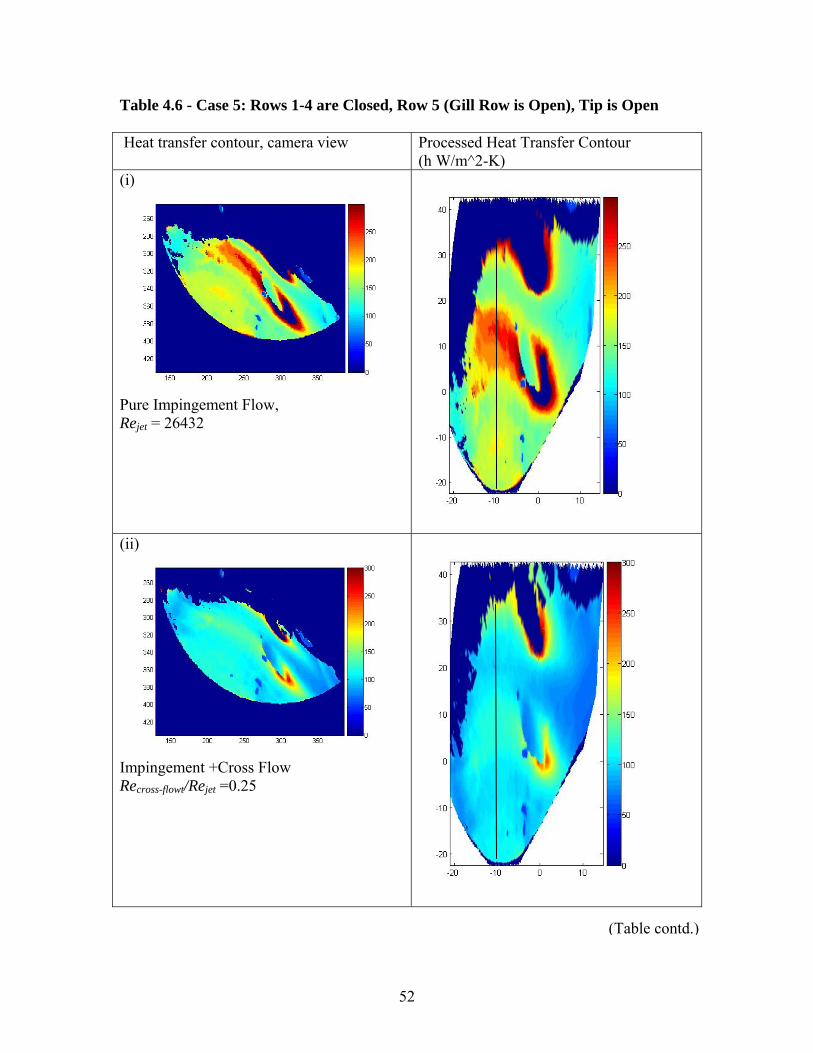
52

Table 4.6 - Case 5: Rows 1-4 are Closed, Row 5 (Gill Row is Open), Tip is Open Heat transfer contour, camera view Processed Heat Transfer Contour

(h W/m^2-K) (i)

Pure Impingement Flow, Rejet = 26432

(ii)

Impingement +Cross Flow Recross-flowt/Rejet =0.25

(Table contd.)

53

(iii)

Impingement +Cross Flow Recross-flowt/Rejet =0.5

Location along Streamwise direction (in mm)

Hea

tTra

nsfe

rCoe

fficien

t(W

/m2 -K

)

-30 -20 -10 0 10 20 30 4050

100

150

200

250

Impingement Flow onlyImpingement Flow Cross Flow-0.25Impingement Flow, Cross Flow-0.5

Location along Streamwise direction vs Heat Transfer Coefficient

Fig 4.5: Line Plot for Case 5

54

Table 4.7 - Case 6: Rows 1-5 are Closed, Tip is Open Heat transfer contour, camera view Processed Heat Transfer Contour

(h W/m^2-K) (i)

Pure Impingement Flow, Rejet = 26468

(ii)

Impingement +Cross Flow Recross-flowt/Rejet =0.25

(Table contd.)

55

(iii)

Impingement +Cross Flow Recross-flowt/Rejet =0.5

Location along Streamwise Direction (in mm)

Hea

tTra

nsfe

rCoe

ffici

ent(

W/m

2 -K)

-30 -20 -10 0 10 20 3050

75

100

125

150

175

200

225

Impingement Flow onlyImpingement Flow, Cross Flow-0.25Impingement Flow, Cross Flow-0.5

Location along Streamwise Direction vs Heat Transfer Coefficient

Fig 4.6: Line Plot for Case 6

56

Fig 4.7: Area selected for average (Blue region)

Table 4.8 - Average value of heat transfer coefficients within the area shown in Fig 4.8

CASE

Area average of heat transfer coefficients (W/m2K)

Case 1(i) 143 Case 1(ii) 128 Case 1(iii) 132 Case 2(i) 162 Case 2(ii) 150 Case 2(iii) 145 Case 3(i) 176 Case 3(ii) 108 Case 3(iii) 117 Case 4(i) 164 Case 4(ii) 119 Case 4(iii) 123 Case 5(i) 213 Case 5(ii) 186

(Table contd.)

57

Case 5(iii) 158 Case 6(i) 113 Case 6(ii) 111 Case 6(iii) 105

The average values of heat transfer are the lowest Case 6 owing to the relative

lack of cross flow when compared to Cases 1-5. The average value of heat transfer seems

to depend on not just the cross flow component but also the film cooling hole

configuration. The exact extent to which each of these components affects the average

value of heat transfer within the selected area cannot be ascertained.

4.2 Discussion of the Results

The magnitude of the maximum heat transfer coefficient and the location of the

stagnation point of the jet depend on the following factors,

• Jet Dimensions

o Height of the Jet

o Diameter of the jet

• Pressure ratio across the impingement hole,

• Number of impingement holes

• Arrangement of impingement holes

• Angle of Impingement of the jet

• Presence of Cross Flow

• Number of rows of Film cooling holes open

• Combination in which the rows of film cooling holes are employed.

Among the above mentioned factors the first four i.e. Jet Dimensions, Pressure ratio,

Number of Impingement Holes and Arrangement of Impingement holes are the same in

58

all the cases and hence can be considered to be constant. The Angle of Impingement is

also constant but its effects on the displacement of the point of maximum heat transfer

(Stagnation Point or Point of Maximum Mass Transfer) are discussed in detail in

relevance to the results obtained. The major distinguishing factors are the final three

factors which are the presence of cross flow, number of film cooling holes open and the

combination in which they are employed. The roles of these factors in the obtained

results are discussed in the subsequent sections.

4.2.1. Jet impingement on an inclined surface

The impingement of a jet on an inclined surface leads to the displacement of the

stagnation point and the point of maximum heat transfer (PMHT) from the geometric

impingement point (GIP) and a reduction in the magnitude of peak heat transfer

coefficient. Also the final heat transfer contour is not symmetric about the axis of

symmetry. This phenomenon has been observed in a number of studies on the

impingement of a jet on oblique surfaces. Sparrow and Lovell, 1980, conducted

experimental studies on the heat transfer characteristics of an obliquely impinging

circular jet. The experiments encompassed a range of incidence angles from normal

impingement to 300 and Reynolds number ranging from 2500 to 30000. It was observed

that any deviation from the normal impingement caused a migration of the point of

maximum heat transfer away from the GIP and a reduced peak heat transfer coefficient.

Also, the displacement of PMHT and reduction in the magnitude of peak heat transfer

coefficient increase with increasing inclination. It was also observed that neither the

maximum pressure point nor the stagnation point may coincide with the PMHT as well as

with each other. Crafton et al., 2006, conducted PIV measurements to locate the

59

stagnation point and the point of maximum pressure for jet angles 150, 300 and 450 angles

at various impingement distances (i.e. height of the jet). The stagnation point and the

point of maximum pressure were found to be located upstream (in the span wise

direction) of the GIP along the axis of symmetry of the jet. These locations of the point of

maximum heat transfer, stagnation point and point of maximum pressure were reported to

be a strong function of the inclination angle and a weaker function of the impingement

distance. Fig 4.8 below shows a comparison of the migration of stagnation point with

respect to inclination angle as recorded by various studies. The various parameters

shown in the Fig 4.8 are sV = Displacement of stagnation point from GIP, H= Height of

the jet, α= Inclination Angle, D= diameter of the jet. All the above studies also indicate a

decrease in the magnitude of maximum heat transfer coefficient. The above results have

been arrived at analytically by Dorrepaal, 1986 and numerically by Garg and Jayaraj,

1988. Figure 4.9 shows the increasing displacement of PMHT and reduction in the

magnitude of peak heat transfer with increasing jet inclination. In the present study the

inclination angle is constant for all the cases and has a value of θ =59.50 (i.e. α= 90-

θ=30.50). A representative cross section is shown in Fig 4.10. The location of the point of

maximum heat transfer seen in the heat transfer contours is a combination of the

inclination angle and the effect of cross flow. It is however difficult to quantify the

individual contribution of these components on the final location of the point of

maximum heat transfer. All the cases (1-6) exhibit this phenomenon to varying degrees.

The movement of the point of maximum heat transfer as a result of the

combination of inclination cross flow and inclination effect is in the range of 0.5D to

O.7D. A more exact figure is difficult to arrive at since pinpointing the location of the

60

Fig 4.8: Deviation of the stagnation point from the geometric impingement point divided by the impingement distance versus α (inclination angle)

Crafton et al, 2006

Fig 4.9: Migration of PMHT and the reduction in magnitude of peak heat tranfer coefficient with increasing jet inclination

Ekkad and Han, 1997

61

stagnation point or the point of maximum heat transfer accurately is not possible using

the current data. Figure 4.11 below shows the movement of the region of impingement

from the GIP for case 5(i). The pitch line for all the holes through which the GIP passes

is shown as a pink line at positive coordinate of 10 mm on the X-axis. The asymmetry of

the heat transfer profile about the axis of symmetry (passing through the GIP) is evident

from Fig 4.11.

Fig 4.10: Displacement of stagnation point

4.2.2. Cross Flow Momentum Versus Jet Momentum

The cross flow component in each of the test cases consists of two components

• Spent flow from the upstream jets

• Independent cross flow introduced in the second and third instances of each case

The cross flow can affect the cooling performance in the following ways:

62

• It provides a buffeting effect to reduce cooling performance by reducing the

impact of the jet flow on the surface.

Fig 4.11: Movement of the Region of Impingement from the GIP for case 5(i).

• It displaces the jet in the direction of the stream and leads to more lateral spread in

the span wise direction. The resulting jet structure is unique and is described in

detail below.

• It can also provide some heat transfer enhancement through increased convective

cooling due to increased mass flow rate the regions further away from the

impingement point of the jet.

The jet as it moves away from the impingement hole acquires the shape of a

horseshoe. This is a result of the interaction of the jet with the external flow. The

intermixing of the emerging jet from the impingement hole with the deflecting cross flow

63

leads to the development of a turbulent layer. As explained in the Chapter one the

peripheral particles of the jet have less velocity than the particles at the core of the jet.

These peripheral particles which are in direct interaction with the cross flow are more

forcefully bent and are moved along more curved trajectories which leads to the

deformation of the circular jet into a horse-shoe structure. Figure 4.12 below illustrates

the development of a counter rotating pair of vortices a.k.a. kidney pair of vortices within

the jet under the influence of cross flow.

As the jet moves away from the impingement hole, the particles of the jet branch out

more and more from the plane of symmetry and the legs of the horse shoe move apart.

The deformation of the jet is observed to a greater or lesser extent in all the cases under

study. The deformed structure of the jet is illustrated for the heat transfer contours of case

4(i) and case 5(i) in Fig 4.13. In the current cases under study, the jet momentum to

external cross flow momentum is in the range of 6 to 8 because of which a clear

development of kidney pair of vortices is not seen for the current height of the jet being

employed. However, the deformation in the imprint clearly shows the effect of the cross

flow. All the effects of cross flow described above compete with each other. There is a

competing effect between the jet momentum and mass flow rate of the cross flow.

As the cross flow increases the ability of the jet to penetrate the cross flow is reduced.

The above three effects act in tandem to give the final HTC contour, wherein, the heat

transfer coefficient at the stagnation point is reduced but a more uniform HTC contour is

obtained. This can be observed from the decrease in the slope of the curve in the line

plots from pure impingement case to cases with increased cross flow.

64

Fig 4.12: Development of a Horseshoe jet with counter rotating pair of vortices under the influence of cross flow, Lincoln, 2001

Also the local circulatory motion (the opposing vortices) within the horse shoe

may contribute to a slight increase in the heat transfer. Such an effect was reported by

Nakabe et al 1998. The exact extent to which each of the above factors affect the

magnitude of heat transfer and the position of PMHT is difficult to predict without further

information on the flow structure within the peanut cavity.

4.2.3. Film Cooling Holes Configuration

There are a total of five rows of film cooling holes on the target surface. Depending

on the number of rows opened and the combination in which these rows are opened, the

stagnation point is shifted accordingly. The combination and number of rows of film

cooling holes used affects the stagnation point and the heat transfer distribution in the

following ways:

65

• The total cross flow within the peanut cavity depends on the number of film

cooling rows kept open. As the number of film cooling holes is reduced there is

an increase in the cross flow. This leads to a greater deflection of the jet and

consequently a greater loss of jet momentum. This leads to a reduction in the peak

heat transfer coefficient. A minor increase in heat transfer away from the

impingement region is observed due to increase in the convective cooling

component.

Fig 4.13: Deformation of the circular jet under the effect of the cross flow for Case 4(i) and Case 5(i)

• The film cooling holes provide a path of lesser resistance to the cross flow when it

is interacting with the jet. Hence the combination in which the rows are used

plays a part in determining the heat transfer distribution. This is the reason why a

higher heat transfer is observed in case 5 when compared to case 2 though in both

66

the cases the same number of rows are kept open. In case 5 since the fourth

showerhead row (the Film Cooling Hole shown in the images belongs to this row)

is closed the cross flow is diverted away from the jet and hence we observe a

higher heat transfer coefficient.

• The location of PMHT of the jet is contingent on the direction in which the cross

flow is diverted. As the flow is diverted through the film cooling holes the PMHT

is deflected toward the hole. This effect is observed strongly in Case 2 where the

entire flow exiting the peanut cavity is routed through the film cooling holes.

4.2.4 Flow Path of Least Resistance

The Jet and the Cross Flow follow a path of least resistance. The Jet and the cross

flow act as inhibitors to each other. Also the flow path of the jet in the peanut cavity

is decided by the configuration of the film cooling holes and the tip condition. For the

tip open cases, a path of lesser resistance towards the tip exists which promotes more

cross flow and hence the impingement point of the jet is moved further downstream.

In case 2, however, the tip is closed and hence the Jet tends to move towards the

corresponding film cooling holes and hence an effective point of impingement is lost.

Therefore we see a decrease in the maximum heat transfer coefficient. Similarly the

configuration of film cooling holes also affects the location of the impingement point

of the jet. There is no direct impact on the location of the impingement point but the

changes in configuration changes the flow path for the spent flow and external cross

flow.

67

Chapter 5

Conclusions

A novel Camera-Endoscope based Liquid Crystal technique was used to study the

heat transfer behavior of a Jet Impingement cooling system under different film

cooling configurations and cross flow conditions. The study was conducted on scaled

model of the leading edge cavity of turbine vane. Heat transfer distribution on the

target surface was obtained for all the cases listed in Table 4.1. A comparison of the

heat transfer distributions indicates that external cross flow has a negative effect on

the peak value of heat transfer but creates a more uniform distribution. This trend is

observed in all the cases. The film cooling configuration plays a significant role in the

determination of the location of the impingement zone and the distribution of heat

transfer. Case 5 exhibits a higher heat transfer and a more uniform distribution than

Case 1 though both have the same number of film cooling rows open. The peak heat

transfer value in each of the cases seems to depend more on the extent of cross flow

than on the film cooling configuration. Closing the tip seems to be unsuitable for this

geometry since the effective impingement of the jet is lost as illustrated in Case 2

although there is an increase in the peak heat transfer. However, this condition might

be remedied by displacing the impingement zone away from the film cooling hole.

This may be achieved by either shifting the impingement holes with respect to the

film cooling holes or by altering the geometry of the target surface.

A further study of the flow structure within the peanut cavity is required to

determine the exact effect of the test parameters on the Impingement location and to

determine the quantify the suggested alterations in the geometry.

68

References

1. www.lag.ensieg.inpg.fr/bouziani/Research2.htm

2. http://www.me.umn.edu 3. Gas Turbine Heat Transfer and Cooling technology, Han J.C., Dutta S, Ekkad

S.V., Taylor and Francis, 2000

4. Bruchez, J. P. and Goldstein, R. J., 1975, "Impingement Cooling from a Circular Jet in a Crossflow," Int. J. of Heat Mass Transfer, Vol. 13, 1975, 719-730.

5. Chance J. L., 1974, "Experimental Investigation of Air Impingement Heat

Transfer under an Array of Round Jets," TAPPI vol. 57, no. 6, pp. 108-112

6. Crafton J, Campbell C, Elliott G, Sullivan J, 2006, ‘The impingement of sonic and sub-sonic jets onto a flat plate at inclined angles’, Experiments in Fluids, Springer-Verlag, No. 41, pg 699-710

7. Downs, S. J., and James, E. H., 1987, "Gas Impingement Heat Transfer - a

Literature Survey," ASME Paper No. 87-HT-35.

8. Dorrepaal J.M., 1986,‘An exact solution of the Navier–Stokes equation which describes non-orthogonal stagnation-point flow in two dimensions’, J Fluid Mech 163, pg 141–147

9. Ekkad, S. V., and Han, J. C., 1997, " Detailed Heat Transfer Distributions in

Two-Pass Square Channels with Rib Turbulators," Int. J. Heat and Mass Transfer, Vol.40, No. 11, pp.2525-2537.

10. Florschuetz, L. W., 1982, "Jet Array Impingement Flow Distribution and Heat Transfer Characteristics," NASA CR 3630.

11. Florschuetz, L. W., Berry, R. A., and Metzger, D.E., 1980, "Periodic Streamwise

Variation of Heat Transfer Coefficients for Inline and Staggered Arrays of Circular Jets with Crossflow of Spent Air," J. of Heat Transfer, Vol. 102, No.I, pp. 132-137.

12. Florschuetz, L. W., Truman, C. R., and Metzger, D.E., 1981, "Streamwise Flow

and Heat Transfer Distribution for Jet Impingement with Crossflow," J. of Heat Transfer, Vol. 103, No.2, pp. 337-342.

13. Florschuetz, L. W., Metzger, D.E., Su, C.C., Isoda, Y., Tseng, H. H., 1984, "Heat

Transfer Characteristics for Jet Array Impingement with Initial Crossflow," J. of Heat Transfer, Vol. 106, No.l, pp. 34-41

69

14. Florshuetz, L.W., Metzger, D.E., and Truman, C.R., 1981, “Jet Array Impingement with Crossflow Correlation of Streamwise Resolved Flow and heat Transfer Distributions,” NACA CR-3373,.

15. Foss J.F., Kleis S.J., 1972,‘The oblique impingement of an axisymmetric jet’,

NASA Technical Report 23-004-068

16. Galant S. and Martinez G., 1982, "Crossflow Influence upon Impingement Convective Heat Transfer in Circular Arrays of Jets, A General Correlation," Proceedings of the 7 th International Heat Transfer Conference, pp. 343 -348.

17. Garg, V. K., Jayaraj S, 1988, ‘Boundary layer analysis for two-dimensional slot

jet impingement on inclined plates’, Trans. of the ASME, Vol 110, pg 577-582

18. Gau, C and Chung, C.M., 1991, “Surface curvature Effect on Slot-Air-jet Impingement Cooling Flow and Heat Transfer Process,” Trans. of the ASME, Vol. 113, pp. 858–864.

19. Goldstein, R. J. and Timmers, J. F., 1982, "Visualization of Heat Transfer from

Arrays of Impinging Jets," Int. J. Heat and Mass Transfer Vol. 25, Dec. 1982, pp 1857-1868

20. Holdeman J. D., 1983, "Perspectives on the Mixing of a Row of Jets With A

Confined Crossflow," Lewis Research Center.

21. Huang, G. C., 1963, "Investigation of Heat Transfer Coefficients for Air Flow through Round Jets Impinging Normal to a Heat Transfer Surface," ASME Journal of Heat Transfer, Vol.85, 1963, pp. 237-243.

22. Huang, P. G., Mujumdar, A.S. and Douglas, W.J., 1984, "Numerical Prediction of

Fluid Flow and Heat Transfer Under a Turbulent Impinging Slot Jet with Surface Motion and Crossflow," ASME paper 84-WA/HT-33.

23. Huang, Y., Ekkad, S. V., and Han, J.C., 1998, "Detailed Heat Transfer

Distributions Under an Array of Orthogonal Impinging Jets," AIAA J. of Thermophysics and Heat Transfer, Vol. 12, No. 1, pp. 73-78.

24. Humber, A.M., and Viskanta, R., 1994, "Comparison of convective Heat Transfer

to Perimeter and Center Jets in a Confined, impingement Array of Axis-symmetric Air Jets," International Journal of Heat and Mass Transfer, vol. 37, pp. 3025-3030.

25. Kercher, D. M. and Tabakoff, W., 1969, "Heat Transfer by a Square Array of

Round Air Jets Impinging Perpendicular to a Flat Surface Including the Effect of Spent Air," ASME paper 69-GT-4, March, 1969.

70

26. Kline, S. J. and McClintock, J., 1953, "Describing Uncertainties in Single-Sample Experiments," Mechanical Engineering, Vol. 75, pp. 3-8

27. Lin, M., Wang, T. and Bunker, R.S., 2000, "Flow and Heat transfer of Confined

Impingement Jets Cooling", ASME Turbo Expo, Paper #2000-GT-223

28. Lincoln P.E. , 2001, ‘A Parametric Study of Jet/Vortex Interactions in the AMRL Water Tunnel’, Aeronautical and Maritime Research Laboratory DSTO-TR-1209

29. Livingood, J.N.B., and Hrycak, P., 1973, "Impingement Heat Transfer from

Turbulent Air Jets to Flat Plates - A Literature Survey," NASA TM X-2778.

30. Martin, H., 1977, "Heat and Mass Transfer between Impingement Gas Jets and Solid Surfaces," Advances in heat Transfer, Vol. 13, Academic Press, New York, pp. 1-60.

31. Metzger, D. E., Yamashita, T., and Jenkins, C. W., 1969, "Impingement Cooling

of Concave Surfaces with Lines of Circular Air Jets," Journal of Engineering of Power, Vol. 91, pp. 149-152.

32. Nakabe K et al, 1998,‘Generation of longitudinal vortices in internal flows with

an inclined impinging jet and enhancement of target plate heat transfer’, International Journal of Heat and Fluid Flow, Vol 19, pg 573-581

33. Saunter, M., Clouser, S., and Han, J. C., “Determination of Surface Heat Transfer

and Film Cooling Effectiveness in Unsteady Wake Flow Conditions.” AGARD Conference Proceedings 527, pp. 6-1 to 6-12, 1992

34. Sparrow E.M., Lovell B.J., 1980, ‘Heat Transfer Characteristics of Obliquely

Impinging Circular Jet’, Trans. of the ASME, Vol 102, pg 202-209

35. Taslim, M.E., Setayeshgar, L., 2001, ‘Experimental Leading-Edge Impingement Cooling Through Racetrack Crossover Holes’, ASME, Paper # 2001-GT-0153,

36. Taslim, M.E., Setayeshgar, L. and Spring, S.D. , 2001, ‘An Experimental

Evaluation of Advanced Leading Edge Impingement Cooling Concepts,’ J. of Turbomachinery, Vol.123, No. 2, pg 147-153

37. Van Treuren, K. W., Wang, Z., Ireland, P. T., and Jones, T. V., 1994, "Detailed

Measurements of Local Heat Transfer Coefficient and Adiabatic Wall Temperature Beneath an Array of Impingement Jets," Journal of Turbomachinery, Vol. 116, No. 2, 1994, pp. 369-374.

38. Viskanta, R., 1993, "Heat Transfer to Impinging Isothermal Gas and Flame Jets,"

Experimental Thermal and Fluid Science, Vol. 6, pp. 111-134.

71

Vita

Amar Jeetendra Panchangam Nivarthi was born in May 1982, to Mr. Rama

Murthy Panchangam Nivarthi and Ms. Sulochana Panchangam Nivarthi in Anantapur,

India. He attended St. Anthony’s High School and finished his Intermediate in

Mathematics and Science from St. Mary’s Junior College. He then earned his Bachelor of

Engineering degree in Mechanical Engineering from University College of Engineering,

Osmania University, Hyderabad, India. Amar then pursued his Master of Science in

Mechanical Engineering from Louisiana State University, Baton Rouge, under the

guidance of Dr. Shengmin Guo and Dr. Sumanta Acharya. Having fulfilled the

requirements set by the Graduate School and the Department of Mechanical Engineering

Amar will graduate in May 2008.