modeling single-phase and boiling liquid jet impingement cooling

National Renewable Energy Laboratory Innovation for Our Energy Future

A national laboratory of the U.S. Department of EnergyOffice of Energy Efficiency & Renewable Energy

NREL is operated by Midwest Research Institute Battelle Contract No. DE-AC36-99-GO10337

Modeling Single-Phase and Boiling Liquid Jet Impingement Cooling in Power Electronics S.V.J. Narumanchi, V. Hassani, and D. Bharathan

Technical Report NREL/TP-540-38787 December 2005

Modeling Single-Phase and Boiling Liquid Jet Impingement Cooling in Power Electronics S.V.J. Narumanchi, V. Hassani, and D. Bharathan

Prepared under Task No. FC05.7000

Technical Report NREL/TP-540-38787 December 2005

National Renewable Energy Laboratory 1617 Cole Boulevard, Golden, Colorado 80401-3393 303-275-3000 • www.nrel.gov

Operated for the U.S. Department of Energy Office of Energy Efficiency and Renewable Energy by Midwest Research Institute • Battelle

Contract No. DE-AC36-99-GO10337

NOTICE

This report was prepared as an account of work sponsored by an agency of the United States government. Neither the United States government nor any agency thereof, nor any of their employees, makes any warranty, express or implied, or assumes any legal liability or responsibility for the accuracy, completeness, or usefulness of any information, apparatus, product, or process disclosed, or represents that its use would not infringe privately owned rights. Reference herein to any specific commercial product, process, or service by trade name, trademark, manufacturer, or otherwise does not necessarily constitute or imply its endorsement, recommendation, or favoring by the United States government or any agency thereof. The views and opinions of authors expressed herein do not necessarily state or reflect those of the United States government or any agency thereof.

Available electronically at http://www.osti.gov/bridge

Available for a processing fee to U.S. Department of Energy and its contractors, in paper, from:

U.S. Department of Energy Office of Scientific and Technical Information P.O. Box 62 Oak Ridge, TN 37831-0062 phone: 865.576.8401 fax: 865.576.5728 email: mailto:[email protected]

Available for sale to the public, in paper, from: U.S. Department of Commerce National Technical Information Service 5285 Port Royal Road Springfield, VA 22161 phone: 800.553.6847 fax: 703.605.6900 email: [email protected] online ordering: http://www.ntis.gov/ordering.htm

Printed on paper containing at least 50% wastepaper, including 20% postconsumer waste

http://www.osti.gov/bridge

mailto:[email protected]

mailto:[email protected]

http://www.ntis.gov/ordering.htm

Executive Summary

Liquid jet impingement is actively being explored for cooling power electronics components – in particular, insulated gate bipolar transistors (IGBTs) found in inverters of hybrid automobiles. This study is divided into two parts – one involving single-phase jets and the other involving boiling jets. For boiling jets, nucleate boiling is the regime considered in this study since this is the most feasible range of operation for electronic cooling applications.

For single-phase jets, we have examined the average simulated chip-surface heat transfer coefficients obtained from the different jet impingement configurations available in the literature. This includes submerged, confined and submerged, and free-surface jets. Both single and multiple jets have been explored. The submerged 9-jet configuration, closely followed by the single confined submerged jet, yields the best heat transfer coefficients of all the configurations considered. Computational fluid dynamics (CFD) simulations were also performed in the CFD code FLUENT in order to validate the code against some existing experimental data in the literature. A reasonable match was found between experimental results and CFD predictions. IGBT package simulations were also performed with glycol-water jets. These simulations suggest that provided issues related erosion and corrosion are addressed, and with further heat transfer enhancement techniques, glycol-water jets at 105°C inlet temperatures can dissipate heat fluxes of up to 150-200 W/cm2.

Extensive experimental data for boiling jets in the nucleate boiling regime also exists in the literature. CFD simulations were also performed with boiling jets. A user defined function was incorporated in FLUENT in order to enable these computations. The code was again validated against existing experimental data in the literature. At this point, it is not entirely clear which fluid would be most feasible for automotive power electronics cooling applications in the boiling regime. Problems related to freezing rule out the use of both water and glycol-water mixture in the boiling regime. Surprisingly, in the context of cooling the IGBT package, CFD results with water as the fluid revealed that boiling jets do not provide any significant (less than 12 %) enhancements over non-boiling jets in terms of maximum temperatures in the solid domain. But it should be cautioned that these conclusions are only for this particular geometry and problem.

iii

Table of Contents

Executive Summary ....................................................................................................................... iii List of Tables ...................................................................................................................................v List of Figures ................................................................................................................................ vi List of Select Symbols and Abbreviations................................................................................... viii Objectives ........................................................................................................................................1 Part I: Single-Phase Liquid Jets .......................................................................................................2

1. Introduction..............................................................................................................................2 2. Single-Phase Liquid Jet Correlations.......................................................................................3

2.1 Different Correlations ........................................................................................................3 2.2 Results from Experimental Correlations............................................................................7

3. CFD Modeling of Single-Phase Liquid Jets: Validation with Experiments ..........................15 4. IGBT Package Simulations....................................................................................................18

4.1 Simulations with Glycol-Water (50%-50%) Mixture......................................................21 4.2 Simulations with Water....................................................................................................23

5. Other Considerations .............................................................................................................24 5.1 Pressure Drop Associated with Jets .................................................................................24 5.2 Erosion Due to Impinging Jets.........................................................................................25

6. Summary and Conclusions for Single-Phase Jets..................................................................27 Part II: Jets Involving Nucleate Boiling.........................................................................................28

7. Introduction............................................................................................................................28 8. Results from Correlations for Nucleate Boiling and CHF.....................................................31

8.1 Nucleate Boiling ..............................................................................................................31 8.2 Critical Heat Flux.............................................................................................................31

9. CFD Modeling of Jets in the Nucleate Boiling Regime: Validation with Experiments ........35 9.1 Validation with Experimental Study of Katto and Kunihiro [33]....................................35 9.2 Impact of Jet Orientation .................................................................................................39 9.3 Impact of Nozzle Diameter..............................................................................................39 9.4 Validation with Zhou and Ma [28] Experimental Study .................................................40

10. IGBT Package Simulations with Boiling Jets......................................................................42 11. Summary and Conclusions ..................................................................................................47

Acknowledgments..........................................................................................................................47 Appendix A: Properties of Various Fluids (from Aspen)..............................................................48 Appendix B: Eulerian Multiphase Model Description ..................................................................53 References......................................................................................................................................57

iv

List of Tables Table 2.1: Fluid (water) properties at 25°C .....................................................................................7 Table 3.1: Comparison between results from experimental correlations and CFD (FLUENT)....17 Table 4.1: Properties of water and glycol-water mixture at 105°C; water is at an operating

pressure of 3.6e+05 Pa to prevent boiling at 105°C, while glycol-water mixture is at 1.013e+05 Pa (1 atm) ....................................................................................................20

Table 4.2: Properties of different solid layer constituent materials at 105°C................................20 Table 4.3: Heat transfer results for the different cases ..................................................................21 Table 9.1: Properties of water and R-113 at 1 atmosphere pressure (1.013e+05 Pa)....................36 Table 9.2: Impact of gravity on the thermal predictions for the case of 100 W/cm2 (Katto and

Kunihiro [33])................................................................................................................39 Table 9.3: Impact of nozzle diameter on the thermal predictions for the case of 100 W/cm

(Katto and Kunihiro [33])2

..............................................................................................40Table 10.1: Properties of water at a pressure of 1.35e+05 Pa (1.3 atm)........................................44 Table 10.2: Summary of results obtained from IGBT package simulations..................................46

v

List of Figures Fig. 2.1: Different jet impingement configurations (taken from [13]): (a) free-surface jet,

(b) submerged jet, (c) confined submerged jet ..............................................................4 Fig. 2.2: Results for average chip-surface heat transfer coefficients from empirical correlations

for single circular jets.....................................................................................................8 Fig. 2.3: Results for the average chip-surface heat transfer coefficients from empirical

correlations for multiple circular jets.............................................................................9 Fig. 2.4: Results from empirical correlations for havg vs. the mass flow rate for single and

multiple jets....................................................................................................................9 Fig. 2.5: Impact of number of jets for submerged and free-surface configurations

(Womac et al. [5,6]) .....................................................................................................10 Fig. 2.6: Impact of nozzle pitch (Pn) for multiple submerged and free-surface jets (4 jets –

Womac et al. [6]) .........................................................................................................12 Fig. 2.7: Impact of SNP on the average chip-surface heat transfer coefficients for confined jet

configurations: (a) havg vs. mass flow rate, (b) havg vs. SNP/d.......................................14 Fig. 3.1: Free-surface jet (Womac et al. [5]) configuration .......................................................15 Fig. 3.2: Submerged jet (Womac et al. [5]) configuration .........................................................16 Fig. 3.3: Confined submerged jet (Garimella et al. [11]) configuration ....................................16 Fig. 4.1: IGBT half-bridge structure ..........................................................................................18 Fig. 4.2: Low-resistance IGBT structure....................................................................................19 Fig. 4.3: IGBT structure with dimensions..................................................................................19 Fig. 4.4: Axisymmetric domain used for the IGBT package simulation ...................................20 Fig. 4.5: Velocity contours in the domain with glycol-water.....................................................22 Fig. 4.6: Temperature contours in the domain with glycol-water at Tinlet = 105°C, vinlet = 8 m/s,

and 90 W/cm2 heat dissipation in the silicon die .........................................................22 Fig. 7.1: General boiling curve for saturated liquids..................................................................30 Fig. 7.2: Mechanism by which critical heat flux occurs ............................................................30 Fig. 8.1: Nucleate boiling curve for different fluids and configurations....................................32 Fig. 8.2: Comparison of results from different CHF correlations ..............................................32 Fig. 8.3: CHF for different saturated fluids from Monde’s correlation .....................................33 Fig. 8.4: Impact of subcooling on CHF with Monde’s correlation for FC72.............................34 Fig. 8.5: Impact of multiple jets on CHF with Monde’s correlation for saturated FC72...........34 Fig. 9.1: Domain used for the Katto & Kunihiro [33] validation study.....................................37 Fig. 9.2: Comparison of boiling curve from experiments (Katto and Kunihiro [33]) and CFD

modeling ......................................................................................................................37 Fig. 9.3: Vapor volume fraction for two cases: 50 W/cm2 (left) and 100 W/cm2 (right)...........38 Fig. 9.4: Wall superheat for two cases: 50 W/cm2 (left) and 100 W/cm2 (right) .......................38 Fig. 9.5: Liquid temperature in the domain for two cases: 50 W/cm2 (left) and 100 W/cm2

(right) ...........................................................................................................................38 Fig. 9.6: Domain for the Zhou and Ma [28] validation study ....................................................41 Fig. 9.7: Boiling curves from experiments and CFD predictions for the Zhou and Ma case [28]

with jet inlet velocities of 0.41 m/s and 11.36 m/s ......................................................41 Fig. 10.1: Axisymmetric domain used for the IGBT package simulation ...................................43 Fig. 10.2: Velocity contours in the domain ..................................................................................43 Fig. 10.3: Temperature contours in the domain - 45 W/cm2 (left) and 90 W/cm2 (right)...........44

vi

Fig. 10.4: Contours of vapor volume fraction - 45 W/cm2 (left) and 90W/cm2 (right) ...............44 Fig. 10.5: Temperature contours in the domain with boiling (left) and without boiling (right) –

for 45 W/cm2................................................................................................................45 Fig. 10.6: Temperature contours in the domain with boiling (left) and without boiling (right) –

for 90 W/cm2................................................................................................................46

vii

List of Select Symbols and Abbreviations

A Area of the target plate, m2

Acorr Area on the target plate corresponding to a single jet, m2

Ar Area ratio

C1, C2 Constants

CP Specific heat, J/KgK

d Jet diameter, m

D Target equivalent diameter, m

f Friction factor

h Heat transfer coefficient, W/m2K

hfg Latent heat, J/Kg

IGBT Insulated-gate bipolar transistor

k Thermal conductivity, W/mK

l Length of the side of a square chip, m

lN Length of the nozzle, m

L Average length of the wall jet region, m

Le Length of nozzle unit cell for an array, m

m,n Exponents

N Number of jets in a multiple jet configuration

Nu Nusselt number

P Power required per unit area, W/m2

Pn Nozzle pitch, m

Pr Prandtl number

qq ′′, Heat flux, W/cm2

R Equivalent radius of the target plate, m

Re Reynolds number

SNP Nozzle-to-target separation, m

u Liquid velocity, m/s

v Jet velocity at the nozzle exit, m/s

V& Flow rate, m3/s

viii

Greek symbols

Jα Relative nozzle area

ε Subcooling parameter

p∆ Pressure drop, Pa

T∆ Temperature difference, K

µ Dynamic viscosity, Ns/m2

ρ Density, Kg/m3

σ Surface tension, N/m

Subscripts

avg Average

CHF Corresponding to critical heat flux

d Jet diameter

di Jet diameter at the impingement plane

f Corresponding to fluid

J Nozzle exit value

l Length of the side of a square chip

l Corresponding to liquid

L Average length of the wall jet region

NP Nozzle-to-target

sat Corresponding to saturation

sub Corresponding to subcooling

v Corresponding to vapor

ix

Objectives Jet impingement has been an attractive cooling option in a number of industries over the past

few decades. Over the past 15 years, jet impingement has been explored as a cooling option in microelectronics. Recently, interest has been expressed by the automotive industry in exploring jet impingement for cooling power electronics components. The main purpose of this technical report is to explore from a modeling perspective both single-phase and boiling jet impingement cooling in power electronics, primarily from a heat transfer viewpoint. The discussion is from the viewpoint of the cooling of IGBTs (insulated-gate bipolar transistors), which are found in hybrid automobile inverters.

First, single-phase jets are examined. In the literature, single and multiple submerged, confined as well as free-surface jets have been investigated. Empirical correlations for heat transfer from the simulated chip surface have been presented. For single-phase liquid jets, non-dimensional correlations have been fairly well established in the literature.

In this report, we discuss in detail these correlations, as well as the heat transfer results from them, using water as a fluid. Computational fluid dynamics (CFD) modeling is also performed, within the framework of the code FLUENT. The CFD results are compared with experimental data from the literature to validate the numerical results and gain confidence in the CFD predictions. Simulations for the IGBT package are then performed. One of the FreedomCAR goals is to use glycol-water mixture at 105°C inlet temperature and also to dissipate close to 200 W/cm2 from the silicon die of the IGBT package. CFD simulations are presented that demonstrate conditions under which it may be possible to achieve these goals using glycol-water mixture. For comparison, results are also presented with water. Some aspects related to the practical implementation—such as pressure drop, erosion, and corrosion associated with impinging jets—are also discussed briefly.

Second, jets that involve nucleate boiling are examined. Typically, for electronic cooling applications, nucleate boiling is the preferred regime of operation because it involves the lowest wall superheats. As is the case with the single-phase jets, a number of experimental studies have been reported in the literature with submerged and free-surface jets that involve boiling. In the boiling literature, because of the difficult nature of the problem, the correlations are typically all dimensional.

In this report, we present CFD modeling of jets involving nucleate boiling. It is not possible to model boiling jets in the commercially available version of FLUENT, so a user-defined function (UDF) was used to perform these simulations. All the simulations relating to boiling jets are performed in close collaboration with the staff at Fluent, Inc. For nucleate boiling, the Eulerian multiphase model is used. A mechanistic model of nucleate boiling is implemented in a UDF in FLUENT. The numerical predictions are validated against experimental studies on submerged jets involving nucleate boiling. These experimental studies involve water and R-113 as the fluids. After this, IGBT package simulations are reported with a submerged boiling jet of water. To the best of our knowledge, these validations and IGBT package simulations with boiling jets are being reported for the first time. A comparison between single-phase and boiling jets from the heat transfer viewpoint and in the context of cooling the IGBT package is also presented.

1

Part I: Single-Phase Liquid Jets 1. Introduction

Single-phase liquid jets have been studied extensively in the literature [1-4]. These studies include experiments, theoretical analyses, and numerical simulations. Different configurations of impinging jets have been studied, including single free-surface jets [5], multiple free-surface jets [6-8], single submerged jets [5, 9, 10], multiple submerged jets [6, 9], and confined single submerged jets [3, 11-13]. Both planar and circular jets have been studied. In the context of electronic cooling, a large number of experimental correlations have been developed for the local and average heat transfer coefficients on the surface of the simulated chip [1-3]. Most of the simulated chips are either 10 x 10 mm2 or 12.7 x 12.7 mm2. Air jets have also been studied extensively [9]. Some of the non-dimensional heat transfer correlations developed from studies on air jets [9] can be applied to liquid jets also.

Researchers have explored the impact of a vast array of parameters—such as jet velocity, jet diameter, impact angle, nozzle-to-chip spacing, nozzle-to-nozzle spacing, turbulence levels, nozzle shapes, nozzle length, jet pulsations, jet confinement, chip-surface enhancement, and fluid properties—on the chip-surface heat transfer coefficients. All these are covered in detail in comprehensive reviews [1-3, 9].

In hybrid electric cars, inverters perform the DC/AC conversion. These inverters contain a number of insulated-gate bipolar transistors (IGBTs), which function as on/off switches. A substantial amount of power is dissipated by these IGBTs. Each IGBT has a silicon die area of 9 x 9 mm2, with a thickness of 0.25 mm. One goal of this report is to explore and compare the different single-phase jet impingement configurations reported in the literature for cooling these IGBTs.

Typically, the package consists of the silicon die, copper layer, aluminum nitride, copper layer, aluminum base plate, and heat sink. In automotive applications, a 50%-50% mixture of ethylene glycol and water is usually used as a coolant. In this report, we first consider a chip of 10 x 10 mm2 and look at the heat transfer performance of different single-phase jet impingement configurations such as single and multiple free-surface jets, single and multiple submerged jets, and confined jets (see Fig. 2.1, taken from [14]). We restrict ourselves to circular jets at this point. Different empirical correlations from the literature are used to gain insights into the average heat transfer coefficients that can be obtained from the chip surface. Numerical simulations (computational fluid dynamics [CFD]) are performed for some of the configurations reported in the literature. Simple calculations are also performed to understand the pressure drop associated with some of these jet impingement configurations. Another practical concern associated with these systems is erosion. High-velocity jets (> 5 m/s) have the potential to erode the material on which they impinge. We look at approximate numbers for the erosion rates for jets impinging on aluminum and copper.

IGBT package simulations are also performed with glycol-water mixture and water as fluids. The jet inlet velocity temperature is maintained at 105°C, and simulations are performed with two different heat fluxes of 90 and 200 W/cm2.

2

2. Single-Phase Liquid Jet Correlations

Extensive literature exists on single-phase jets (see Introduction). In this section, results are presented for the average chip-surface heat transfer coefficients obtained for different jet configurations. The intent is not to obtain results from all the correlations that appear in the literature. Rather, a few representative correlations, chosen to cover the different types of jet configurations, are presented in this section. These correlations are used because they should be applicable over a fairly wide range of parameters, and they should be able to replicate experimental data of other investigators who studied similar configurations within a reasonable percentage error. Although the motivation for this study is the possible use of single-phase jets for power electronics applications, the information presented could be of use in other applications as well.

2.1 Different Correlations

2.1.1 Martin correlation [9] for a single circular submerged jet

5.055.0

2/1

42.0

)200

Re1(Re2)(Re

/)6/(1.01/1.11)/,/(

)(Re)/,/(Pr

JJJ

NPNP

JNP

F

RddSRd

RddSRdG

FdSRdGNu

+=

⎭⎬⎫

⎩⎨⎧

−+−=

=

(2.1)

2,000 ≤ ReJ ≤ 400,000; 2.5 ≤ R/d ≤ 7.5; 2 ≤ SNP/d ≤ 12

where d = nozzle diameter, SNP = nozzle-to-target separation, R = equivalent radius of the target,

Nu = havgd/k, ReJ = ρ vd/µ, and Pr= µ CP /k.

3

(a) (b)

(c)

Fig. 2.1: Different jet impingement configurations (taken from [13]): (a) free-surface jet, (b)

submerged jet, (c) confined submerged jet 2.1.2 Womac et al. correlation [5] for a single circular submerged jet

This correlation is for the same jet configuration as the Martin correlation [9] presented previously.

22

214.0

/)9.1(2

)9.15.0()9.125.0(

)1(ReRePr

ldA

dldlL

ALlCA

dlCNu

r

rnLr

md

l

π=

−+−=

−+=

(2.2)

Red < 50,000; 1.65 ≤ d ≤ 6.55 mm; 1.5 ≤ SNP/d ≤ 4

where d = nozzle diameter, SNP = nozzle-to-target separation, l = length of the side of the square heat source, L = average length of the wall jet region, l = 12.7 mm, m = 0.5, n = 0.8, C1 = 0.785, C2 = 0.0257, Nul = havgl/k, Red = ρ vd/µ, ReL= ρ vL/µ , and Pr = µ CP /k.

4

2.1.3 Garimella and Rice [11] correlation for a single confined circular submerged jet

11.011.04.0695.0 PrRe160.0

−−

⎟⎠⎞

⎜⎝⎛

⎟⎠⎞

⎜⎝⎛=

dl

dSNu NNP

1.59 ≤ d ≤ 6.35 mm; 4,000 ≤ Re ≤ 23,000; 1 ≤ SNP/d ≤ 5 (2.3) 0.25 ≤ lN/d ≤ 12

05.052.04.0773.0 PrRe164.0

−−

⎟⎠⎞

⎜⎝⎛

⎟⎠⎞

⎜⎝⎛=

dl

dSNu NNP

parameter range is same as above, except 6 ≤ SNP/d ≤ 14

where d = nozzle diameter, SNP = nozzle-to-target separation, lN = length of the nozzle, Nu = havgd/k, Re = ρvd/µ , and Pr = µ CP /k.

2.1.4 Womac et al. correlation [5] for a single circular free-surface jet

22

214.0

/)(2

)5.0()25.0(

)1(ReRePr

ldA

dldlL

ALlCA

dlCNu

ir

ii

rnLr

i

md

li

π=

−+−=

−+=

(2.4)

Redi < 50,000; 1.65 ≤ d ≤ 6.55 mm; 3.5 ≤ SNP/d ≤ 10

where d = nozzle diameter, di = jet diameter in impingement plane, SNP = nozzle-to-target separation, l = length of the side of the square heat source, L = average length of the wall jet region, l = 12.7 mm, m = 0.5, n = 0.532, C1 = 0.516, C2 = 0.491, Nul = havgl/k, Redi = ρ vdi/µ, ReL= ρ vL/µ, and Pr = µ CP /k. 2.1.5 Martin correlation [9] for multiple circular submerged jets

3/2

05.0

6

42.0

Re5.0)(Re

)6/(2.01)2.21(2

),/(

)/6.0

/(1),/(

)(Re),/(),/(Pr

JANJ

JNP

JJJNP

J

NPJNP

ANJJNPJNPAN

F

dSdSG

dSdSK

FdSGdSKNu

=

−+−

=

⎥⎥⎦

⎤

⎢⎢⎣

⎡+=

=⎟⎠⎞

⎜⎝⎛

−

ααα

α

αα

αα

(2.5)

2,000 ≤ ReJ ≤ 100,000; 0.004 ≤ αJ ≤ 0.04; 2 ≤ SNP/d ≤ 12

5

where, αJ = (πd2)/(4Acorr..), d = nozzle diameter, SNP = nozzle-to-target separation, Nu = havgd/k, ReJ = ρ vd/µ, Pr = µ CP /k, AN stands for array of nozzles, and Acorr is the area corresponding to a single jet. 2.1.6 Womac et al. correlation [6] for multiple circular submerged jets

22

214.0

/)9.1(2

]9.1)2/[(]9.12/2[(

)1)((Re)(RePr

ldNA

dLdLL

ALlCA

dlCNu

r

ee

rnLr

md

l

π=

−+−=

−+=

(2.6)

5,000 ≤ Red ≤ 20,000; 0.5 ≤ d ≤ 1.0 mm; 2 ≤ SNP/d ≤ 4; N = 4 or 9 jets; l = 12.7 mm; m =

0.5; n = 0.8; C1 = 0.509; C2 = 0.0363

where, d = nozzle diameter, SNP = nozzle-to-target separation, l = length of the side of the square heat source, L = average length of the wall jet region, Le= length of nozzle unit cell for an array, Nul= havgl/k, Red = ρ vd /µ, ReL= ρ vL/µ,, and Pr= µ CP /k. 2.1.7 Womac et al. correlation [6] for multiple circular free-surface jets

22

214.0

4/)(2

)]2/()2/[()]2/(2/2[(

)1)((Re)(RePr

ldNA

dLdLL

ALlCA

dlCNu

ir

ieie

rnLr

i

md

li

π=

−+−=

−+=

(2.7)

5,000 ≤ Red ≤ 20,000; 0.5 ≤ d ≤ 1.0 mm; 2 ≤ SNP/d ≤ 20; N = 4 or 9 jets; l = 12.7 mm; m =

0.5; n = 0.579; C1 = 0.516; C2 = 0.344

where d = nozzle diameter, di= nozzle diameter at impingement plane, SNP = nozzle-to-target separation, l = length of the side of the square heat source, L = average length of the wall jet region, Le= length of nozzle unit cell for an array, Nul = havgl/k, Redi = ρ vdi /µ,, ReL= ρ vL/µ, and Pr= µ CP /k.

The chip-surface heat transfer results for these configurations have been tabulated in the form of plots. These correlations are used to obtain data for the average heat transfer coefficients from the chip surface. Plots have been generated for the average chip-surface heat transfer coefficient (h) vs. the mass flow rate, as well as h vs. the inlet velocity of the coolant (water). For all these cases, the chip is considered to be 10 x 10 mm2, simulating an IGBT.

6

Table 2.1: Fluid (water) properties at 25°C

ρ (kg/m3) 998 CP (J/kgK)

4,182

µ (Ns/m2) 0.001003k (W/mK) 0.60 Pr 7.0

2.2 Results from Experimental Correlations

In this section we look at the average chip-surface heat transfer coefficients for the different jet impingement configurations. As mentioned in the previous section, the chip is considered to have the dimension 10 x 10 mm2. All results are with water as the impinging fluid, and the properties of water corresponding to a temperature of 298 K (25°C) are chosen (Table 2.1). Figure 2.2 shows the average heat transfer coefficient as a function of the jet inlet velocity for the different single circular jet configurations (see Fig. 2.1). These include single circular submerged jets (Womac et al. [5], Martin [9]), single circular free-surface jets (Womac et al. [5]), and single circular confined and submerged jets (Garimella and Rice [11]). For the submerged circular jet, the diameter d = 1.65 mm, and SNP = 4d. For the free-surface circular jet, the diameter d = 1.65 mm, and SNP = 10d. For the confined and submerged circular jet, the diameter d = 1.65 mm, and SNP = 4d.

For all configurations, the heat transfer coefficient increases with velocity, as expected. For submerged and confined jets, a value of SNP = 4d was chosen so that the chip was within the potential core of the jet. Hence, this distance yields the maximum heat transfer possible from these configurations. For the free-surface jets, the actual value of SNP is less critical, unless the jet inlet velocity is so low that there is a substantial increase in velocity due to gravitational acceleration just prior to impact with the chip surface.

The results from the Martin [9] and Womac et al. [5] correlations for the single submerged circular jets are within 15% over a wide range of velocities. This gives confidence in using both these correlations within their respective ranges of validity. The single free-surface jet yields noticeably lower heat transfer coefficients, especially at higher velocities. This is attributed to splattering of the fluid, which causes the liquid film in the wall jet region to become thin, thereby causing the liquid to heat up owing to the boundary layer reaching the free surface of the liquid film [5]. The single circular confined and submerged jet configuration of Garimella and Rice [11] yields the highest heat transfer coefficients. They [11] postulate that confinement causes fluid recirculation and enhancement in the turbulence levels, thereby increasing the heat transfer from the chip surface. Perhaps confinement also impacts the pressure gradients and the boundary layer development on the chip surface, which in turn could enhance heat transfer.

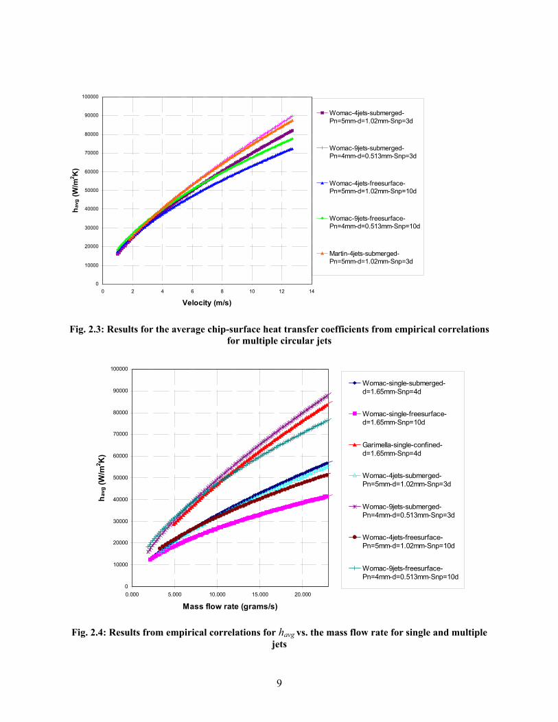
Figure 2.3 shows the results for the average chip-surface heat transfer coefficient as a function of jet velocity, obtained from multiple jet configurations, which includes both free-surface and submerged jets. In this figure, Pn refers to the distance between the nozzles. Results are presented for configurations involving 4 jets as well as 9 jets. For the submerged 4-jet configuration, with jet diameter d = 1.02mm, SNP = 3d, and nozzle pitch Pn = 5 mm, the Womac

7

et al. [5] and Martin [9] correlations yield results which are within 10% for the entire range of velocities presented in Fig. 2.3. This again gives confidence in the use of both the Martin and Womac et al. correlations. All other parameters remaining the same (i.e., number of jets, jet diameter, and Pn), the submerged jets yield higher heat transfer coefficients than free-surface jet configurations, especially at higher velocities. Importantly, at any given velocity, the mass flow rates from the different configurations are not the same.

In Fig. 2.4, the average heat transfer coefficients are plotted against the mass flow rate for all the different jet configurations (single and multiple jet, submerged, free-surface, and confined submerged jets). The following sections examine different aspects of the results.

2.2.1 Comparison between Martin [9] and Womac et al. [5] correlations for submerged circular jets

For the single submerged circular jet with diameter d = 1.65mm and SNP = 4d, the Martin [9] and Womac et al. [5] correlations are within 15%-20% for the entire range of mass flow rates considered (Fig. 2.2). For 4 multiple submerged jets of diameter d = 1.02 mm, SNP = 3d, and Pn =5 mm, the Martin [9] and Womac et al. [6] correlations are again within 15% (Fig. 2.3).

0

10000

20000

30000

40000

50000

60000

70000

80000

90000

100000

0 2 4 6 8 10 12 14

Velocity (m/s)

havg

(W/m

2 K)

Womac-submerged-d=1.65mm-Snp=4d

Womac-freesurface-d=1.65mm-Snp=10d

Martin-submerged-d=1.65mm-Snp=4d

Garimella-confined-d=1.65mm-Snp=4d

Fig. 2.2: Results for average chip-surface heat transfer coefficients from empirical correlations for

single circular jets

8

0

10000

20000

30000

40000

50000

60000

70000

80000

90000

100000

0 2 4 6 8 10 12 14

Velocity (m/s)

havg

(W/m

2 K)

Womac-4jets-submerged-Pn=5mm-d=1.02mm-Snp=3d


Womac-4jets-freesurface-Pn=5mm-d=1.02mm-Snp=10d


Martin-4jets-submerged-Pn=5mm-d=1.02mm-Snp=3d

Fig. 2.3: Results for the average chip-surface heat transfer coefficients from empirical correlations

for multiple circular jets

0

10000

20000

30000

40000

50000

60000

70000

80000

90000

100000

0.000 5.000 10.000 15.000 20.000

Mass flow rate (grams/s)

havg

(W/m

2 K)

Womac-single-submerged-d=1.65mm-Snp=4d

Womac-single-freesurface-d=1.65mm-Snp=10d

Garimella-single-confined-d=1.65mm-Snp=4d





Fig. 2.4: Results from empirical correlations for havg vs. the mass flow rate for single and multiple jets

9

These correlations have an average error of 10%-15%. These correlations were obtained from entirely different studies. In fact, the Martin [9] non-dimensional correlations were derived from studies on air jets. Therefore, this builds confidence in the use of either of these correlations, within their range of applicability.

2.2.2 Comparison between single and multiple submerged circular jet configurations

The 4 circular submerged jet configuration (Womac et al. [6]) yields heat transfer coefficients that are almost the same or slightly lower than the coefficients obtained from the single circular submerged jet configuration (Womac et al. [5]) (Fig. 2.4). However, the 9 circular submerged jet configuration (Womac et al. [6]) yields much larger heat transfer coefficients than the single submerged or 4 submerged jet configurations. This suggests that the arrangement of jets plays a critical role in determining the extent of heat transfer enhancement that can be obtained from multiple jets compared with single jets. When there is a larger number of multiple jets, the number of stagnation zones increases, the interactions between adjacent jets also increase [15, 16], and the wall jet regions decrease. These aspects combine to determine whether there are enhancements in the overall average heat transfer coefficients from the chip surface compared with the single jet. Figure 2.5 shows the average heat transfer coefficient as a function of the number of jets for two different mass flow rates, 10 and 20 grams/s. The results mentioned above are borne out more clearly in this figure.

0

10000

20000

30000

40000

50000

60000

70000

80000

90000

0 1 2 3 4 5 6 7 8 9 10

Number of jets

havg

(W/m

2 K)

Womac-submerged-10grams/s

Womac-submerged-20grams/s

Womac-freesurface-10grams/s

Womac-freesurface-20grams/s

Fig. 2.5: Impact of number of jets for submerged and free-surface configurations (Womac et al.

[5,6])

10

2.2.3 Comparison between single and multiple free-surface circular jet configurations

The 4 jet free-surface configuration of Womac et al. [6] with a pitch Pn = 5 mm yields higher heat transfer coefficients than the single free-surface jet configuration of Womac et al. [5] (Figs. 2.4, 2.5). Again, when the number of jets is increased to 9, the heat transfer coefficients are significantly higher than those corresponding to single free-surface jet and 4 jet configurations. Fig. 2.5 depicts these results for multiple free-surface jets.

2.2.4 Comparison between free-surface and submerged circular jet configurations

The single submerged jet with d = 1.65 mm yields higher heat transfer coefficients than the single free-surface jet of the same diameter, especially at larger mass flow rates (Figs. 2.4, 2.5). Similarly, the submerged 4 jet configuration yields larger heat transfer coefficients than the 4 jet free-surface configuration, all parameters (except SNP) remaining the same. The submerged 9 jet configuration also yields higher coefficients than the free-surface 9 jet configuration at larger mass flow rates. The underlying theme is that at larger mass flow rates, the submerged jet configurations yield higher heat transfer rates than the corresponding free-surface jet configurations (Figs. 2.4, 2.5). Submerged jets are associated with larger levels of fluid mixing and turbulence than free-surface jets. Additionally, with free-surface jets at higher mass flow rates, splashing of the liquid results in decreased film thickness. This decrease in liquid film thickness results in bulk warming of the liquid due to the boundary layers reaching the surface of the liquid film [5, 6]. Below a velocity of 2 m/s (Figs. 2.2, 2.3) or a flow rate of 5 grams/s (Fig. 2.4), free-surface and submerged jets yield similar average heat transfer coefficients.

2.2.5 Effect of nozzle pitch

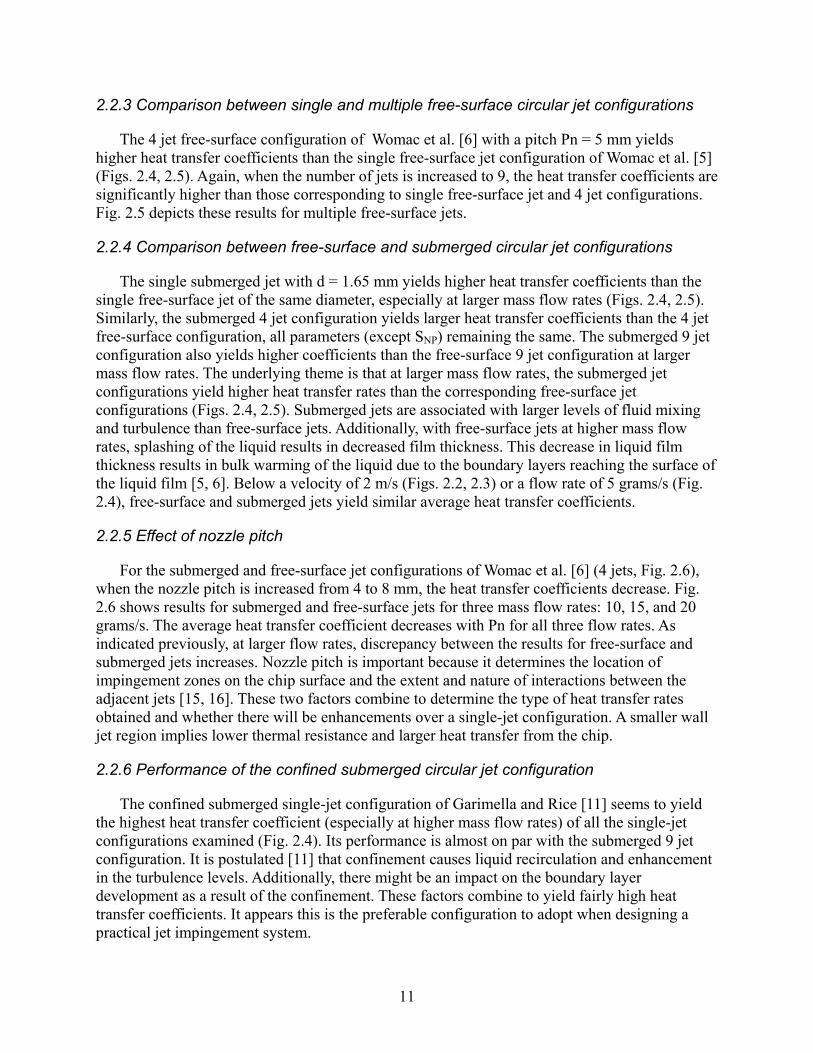
For the submerged and free-surface jet configurations of Womac et al. [6] (4 jets, Fig. 2.6), when the nozzle pitch is increased from 4 to 8 mm, the heat transfer coefficients decrease. Fig. 2.6 shows results for submerged and free-surface jets for three mass flow rates: 10, 15, and 20 grams/s. The average heat transfer coefficient decreases with Pn for all three flow rates. As indicated previously, at larger flow rates, discrepancy between the results for free-surface and submerged jets increases. Nozzle pitch is important because it determines the location of impingement zones on the chip surface and the extent and nature of interactions between the adjacent jets [15, 16]. These two factors combine to determine the type of heat transfer rates obtained and whether there will be enhancements over a single-jet configuration. A smaller wall jet region implies lower thermal resistance and larger heat transfer from the chip.

2.2.6 Performance of the confined submerged circular jet configuration

The confined submerged single-jet configuration of Garimella and Rice [11] seems to yield the highest heat transfer coefficient (especially at higher mass flow rates) of all the single-jet configurations examined (Fig. 2.4). Its performance is almost on par with the submerged 9 jet configuration. It is postulated [11] that confinement causes liquid recirculation and enhancement in the turbulence levels. Additionally, there might be an impact on the boundary layer development as a result of the confinement. These factors combine to yield fairly high heat transfer coefficients. It appears this is the preferable configuration to adopt when designing a practical jet impingement system.

11

0

10000

20000

30000

40000

50000

60000

4 4.5 5 5.5 6 6.5 7 7.5 8

Pn (mm)

havg

(W/m

2 K)

4 submerged jets - 10grams/s

4 freesurface jets - 10grams/s





Fig. 2.6: Impact of nozzle pitch (Pn) for multiple submerged and free-surface jets (4 jets – Womac

et al. [6])

2.2.7 Impact of nozzle-to-target distance (SNP) on the heat transfer performance of confined submerged circular jets

Figure 2.7 shows the impact of nozzle-to-target distance (SNP) on the heat transfer performance of confined submerged jets [11]. Figure 2.7(a) shows the average heat transfer coefficient vs. the mass flow rate for single submerged circular jets—both confined [11] and unconfined [5, 9]. For a jet with a diameter d = 1.65mm, and SNP = 4d, the Womac et al. correlation [5] and Martin correlation [9] yield results that are within 15%-20% of one another, as discussed previously. For the confined submerged jet configuration [11], four different SNP values are considered (Fig. 2.7(a)): SNP = 4d, SNP = 7d, SNP = 10d, and SNP = 14d. The heat transfer coefficients from SNP = 4d and 7d are almost the same. At these values of SNP, the chip is within the potential core of the jet, and there is little difference in the heat transfer performance of the two jets. However, when SNP is increased to 10d, the heat transfer coefficients fall, and there is a further decrease when SNP is increased to 14d. When SNP is increased such that the chip is outside the potential core of the jet, the jet strikes the chip with a much lower velocity, resulting in a decrease in the heat transfer coefficients. Figure 2.7(b) shows clearly the decrease in havg with increasing SNP/d. This trend holds for all three flow rates (10, 15, and 20 grams/s). The kink at SNP/d = 6 occurs because Garimella and Rice [11] present two different correlations, one for SNP/d ≤ 5 and the other for SNP/d > 5. The heat transfer performance of the confined submerged jet [11] with SNP = 14d is similar to the heat transfer performance of the unconfined submerged jet [5, 9] with SNP = 4d (Fig. 2.7(a)).

12

In summary, single-phase jets have the potential to yield fairly high heat transfer coefficients. The results with water jets indicate maximum coefficients on the order of 60,000 W/m2K with a jet inlet velocity of 7 m/s (Fig. 2.2) or a mass flow rate of 15 grams/s (Fig. 2.4). One of the goals in power electronics thermal management is to attain heat transfer coefficients on the order of 60,000 W/m2K in the heat sink. In that sense, single-phase liquid jets seem promising.

13

(a)

0

10000

20000

30000

40000

50000

60000

70000

80000

90000

100000

0 5 10 15 20

Mass flow rate (grams/s)

h avg

(W/m

2 K)

Womac-single-submerged-d=1.65mm-Snp=4d

Martin-single-submerged-d=1.65mm-Snp=4d





(b)

0

10000

20000

30000

40000

50000

60000

70000

80000

90000

3 5 7 9 11 13 15

Snp/d

h avg

(W/m

2 K)

Garimella-singlejet-d=1.65mm-10grams/s



Fig. 2.7: Impact of SNP on the average chip-surface heat transfer coefficients for confined jet

configurations: (a) havg vs. mass flow rate, (b) havg vs. SNP/d

14

3. CFD Modeling of Single-Phase Liquid Jets: Validation with Experiments

To corroborate some of the experimental results reported in the literature, we performed numerical simulations (CFD) for single free-surface [5], submerged [5], and confined submerged jet [11] configurations. The numerical simulations were performed using the commercial CFD code FLUENT, which is based on the finite volume method [17]. No single turbulence model yields results that match experimental data for different types of problems and a wide range of Reynolds numbers. The k-omega model is the most suitable model for this class of impinging jet flows. Hence, for all the results reported here, we employed the standard k-omega turbulence model with the enhanced wall treatment. The y+ values near the wall are maintained close to 1 in accordance with the requirements of using the enhanced wall treatment. Also, all the CFD results presented in this section are independent of the spatial mesh to within 5%. For the free-surface jets, the steady-state implicit volume-of-fluid method [18] is used. In this methodology, we perform a two-phase (air and water) simulation, and the interface between the phases is tracked. All simulations performed are axisymmetric cases. We tried to replicate the experimental conditions as closely as possible.

All the configurations, problem parameters, and results are given in Table 3.1. The heated target plate in all cases is assumed to be a circular disk with area equal to that of the actual target plate used in the experiments. Figure 3.1 shows the domain and representative velocity contours with free-surface jets, while Figs. 3.2 and 3.3 show these with submerged and confined submerged jets, respectively.

Fig. 3.1: Free-surface jet (Womac et al. [5]) configuration

15

Fig. 3.2: Submerged jet (Womac et al. [5]) configuration

Fig. 3.3: Confined submerged jet (Garimella et al. [11]) configuration

The CFD results for average chip-surface heat transfer coefficients indicate that for the single circular submerged jet configurations (Womac et al. [5]), a reasonable match (within 20%) exists with experimental data (obtained from correlations) over a wide range of Reynolds numbers. The discrepancy between CFD predictions and experimental data for single free-surface jets (Womac et al. [5]) is as much as 30% for the high Reynolds number cases. It is possible that for these free-surface jets, the shape of the free surface and the thickness of the liquid film are not being captured accurately at elevated Reynolds numbers. For the submerged confined jet configuration (Garimella and Rice [11]), again a good match is obtained between CFD predictions and experimental data (within 10%) over a wide range of Reynolds numbers.

Overall, we conclude that, for confined and unconfined submerged jets, there is a good match between CFD results and experimental data over a wide range of Reynolds numbers. However, for single free-surface jets, there is some discrepancy between CFD predictions and experimental results at higher Reynolds numbers.

16

Table 3.1: Comparison between results from experimental correlations and CFD (FLUENT) Configuration Problem parameters havg from

correlations (W/m2K)

havg from CFD (FLUENT) (W/m2K)

% difference between FLUENT and correlation

v = 3 m/s, d = 3.1 mm, D = 14.3 mm, SNP =

Re4d, d = 9,300 27,300 26,400 3

Single circular submerged jet (Womac et al. [5])

v = 15 m/s, Red = 46,400 69,300 81,400 16

v = 1 m/s, d = 3.1 mm, D = 14.3 mm, SNP =

Re4d, d = 3,100 11,500 14,000 20

v = 3 m/s, Red = 9,300 19,600 22,500 14

Single circular free-surface jet (Womac et al. [5])

v = 15 m/s, Red = 46,400 45,700 61,000 29

v = 1.3 m/s, d = 3.2mm, D = 11.3 mm, SNP = 4d, Red = 4,100

18,300 19,200 5

v = 3.3 m/s, Red = 10,300 34,800 34,800 0

Single circular submerged and confined jet (Garimella and Rice [11])

v = 7.0 m/s, Red = 22,100 59,100 54,500 8

17

4. IGBT Package Simulations

In Section 3, we demonstrated that the CFD code FLUENT can be used with a reasonable degree of confidence for modeling single-phase submerged liquid jets. In this section, we model jet impingement cooling of the IGBT package. Figure 4.1 shows the IGBT half-bridge structure. This structure has 12 IGBTs and 6 diodes. Typically, there are 3 half-bridges in an inverter for an automobile, so in all there are 36 IGBTs and 18 diodes. In this report, we focus on modeling one IGBT.

Figure 4.2 shows the low-resistance IGBT structure in which the aluminum plate is cut through to provide a path for direct impingement of the jet onto the copper layer of the DBC stack. The dimensions of the IGBT structure are indicated in Fig. 4.3. The silicon die is 0.25 mm thick, the solder layer is 0.05 mm thick, the AlN (aluminum nitride) layer is 0.64 mm thick, and the copper layers in the DBC stack are 0.35 mm thick. In this report, the thickness of the aluminum cold plate is taken to be 6 mm.

Figure 4.4 demonstrates the axisymmetric domain used for the IGBT package simulation. The jet impinges directly onto the copper wall as shown in Fig. 4.4. The jet diameter is taken to be 1.5 mm, and the distance between the jet inlet and the copper wall is 6 mm, which means that the target surface is within 4 diameters from the nozzle exit. As shown in Sections 2 and 3, for submerged jets, this means that the target surface is within the potential core of the jet. Because an axisymmetric domain is used, the radius of the silicon layer is 5.1 mm, the radii of the copper and AlN layers are 11.3 mm, and the radius of the outside of the aluminum layer is 13 mm. All the outside edges of the solid layers are adiabatic as indicated in Fig. 4.4.

Numerical simulations are carried out with glycol-water mixture (50%-50%) and water. The properties of the fluid are indicated in Table 4.1. A jet inlet temperature of 105°C is chosen, in accordance with the one of the essential requirements of the FreedomCAR Program. Simulations are performed with water for comparison. At atmospheric pressure (1.01325e+05 Pa), water boils at 100°C, so during the simulations with water the operating pressure is maintained at 3.61e+05 Pa. At this operating pressure, the saturation temperature of water is 140°C, so water does not boil at 105°C. The material properties of the solid layers are given in Table 4.2. Below we discuss the results obtained from the numerical simulations. Again, the k-omega turbulence model with enhanced wall treatment is used, consistent with the approaches described in Section 3. The numerical results presented below are expected to be mesh independent to within 5%.

Fig. 4.1: IGBT half-bridge structure

18

Fig. 4.2: Low-resistance IGBT structure

Fig. 4.3: IGBT structure with dimensions

19

CopperAluminum

Pressure outlet

Adiabatic

Jet inlet

Fig. 4.4: Axisymmetric domain used for the IGBT package simulation Table 4.1: Properties of water and glycol-water mixture at 105°C; water is at an operating pressure

of 3.6e+05 Pa to prevent boiling at 105°C, while glycol-water mixture is at 1.013e+05 Pa (1 atm)

Glycol-water mixture

Water

Density, kg/m3 1,008 955 Specific heat, J/kg-K 3,644 4,226 Dynamic viscosity, Ns/m2 0.000656 0.000267 Thermal conductivity, W/mK 0.43 0.68

Table 4.2: Properties of different solid layer constituent materials at 105°C

Aluminum Al. Nitride Copper Silicon Solder Density, kg/m3 2,719 3,260 8,960 2,330 8,904 Specific heat, J/kg-K 870 740 377 700 173 Thermal conductivity, W/mK 235 140 394 116 36

20

4.1 Simulations with Glycol-Water (50%-50%) Mixture

As shown in Table 4.3, two different cases are examined, one in which the heat dissipation in the silicon die is effectively 90 W/cm2 (corresponding to 72.9 W in a single IGBT) and the other in which the heat dissipation is 200 W/cm2 (corresponding to 162 W in a single IGBT). A heat dissipation of 200 W/cm2 is close to the upper limit of one of the important goals of the FreedomCAR Program, which is the reason we examine it here. For the case involving 90 W/cm2, we use a jet velocity of 8 m/s, while for the case involving 200 W/cm2 a jet velocity of 20 m/s is used. We use these velocities to limit the maximum temperatures in the domain to as close to 125°C as possible. This maximum temperature of 125°C is another important goal of the FreedomCAR Program. As already indicated, the jet inlet temperature is at 105°C, in line with another FreedomCAR goal.

Table 4.3: Heat transfer results for the different cases

Glycol-water mixture Water

90 W/cm2 200 W/cm2 90 W/cm2 200 W/cm2

Jet velocity, m/s 8 20 8 20 Tinlet, °C 105 105 105 105 Tmax, °C 125 135 119 127 hcopper, W/m2K 39,000 75,700 74,200 157,300 haluminum, W/m2K 19,800 40,500 37,100 76,500

4.1.1 Case with 90 W/cm2

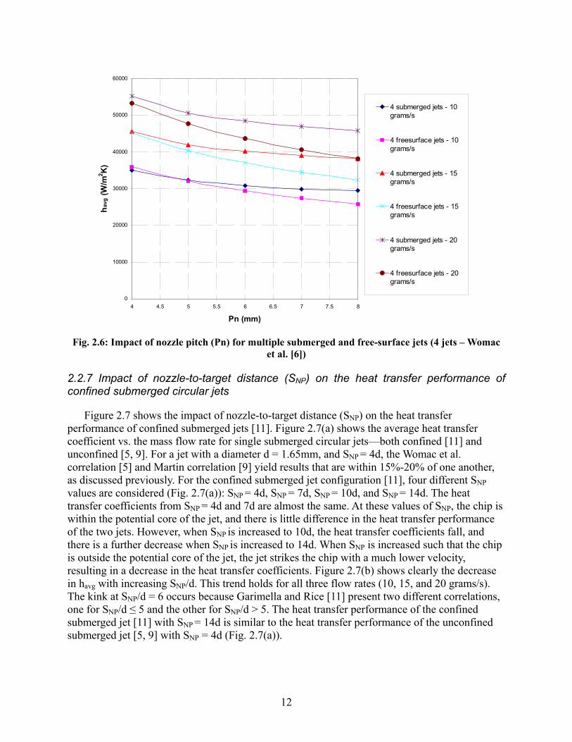
Figures 4.5 and 4.6 show the velocity and temperature contours, respectively, in the domain for the case in which the jet inlet velocity is 8 m/s and the heat dissipation in the silicon die is 90 W/cm2 (second column of Table 4.3). For this case, the heat transfer coefficients from the copper and aluminum surfaces are indicated in Table 4.3 (39,000 and 19,800 W/m2K, respectively). Because the enhanced wall treatment is used, the values of y+ near the copper and aluminum walls are driven close to a value of 1. These heat transfer coefficients are also in line with the values indicated by correlations from the literature [5, 9]. The maximum temperature in the domain is 125°C. For these single-phase flows, the mechanism of heat transfer is forced convection.


In this case, the heat dissipated in the die is 200 W/cm2, and a jet velocity of 20 m/s is used (column 3 of Table 4.3). The maximum temperature in the domain is 135°C. This is an important result; it gives us a sense of the velocities required to dissipate heat fluxes on the order of 200 W/cm2 while maintaining temperatures close to the program goals. The velocity required is high.

21

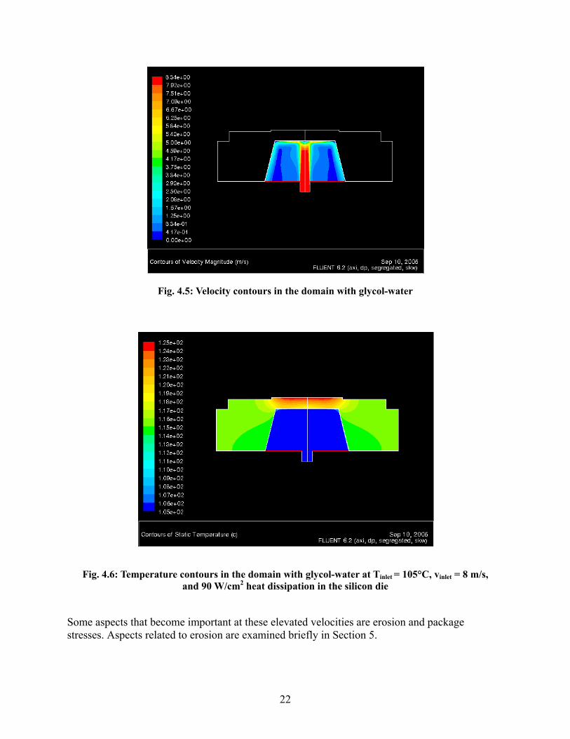
Fig. 4.5: Velocity contours in the domain with glycol-water

Fig. 4.6: Temperature contours in the domain with glycol-water at Tinlet = 105°C, vinlet = 8 m/s, and 90 W/cm2 heat dissipation in the silicon die

Some aspects that become important at these elevated velocities are erosion and package stresses. Aspects related to erosion are examined briefly in Section 5.

22

Probably the way to dissipate such high heat fluxes without using excessively high velocities would be to enhance the heat transfer coefficients from the solid surfaces (copper and aluminum). Some possibilities are surface enhancements and the use of pulsating/self-oscillating jets. In the literature, surface enhancements [19] and jet pulsations [20, 21] have been demonstrated to yield significant enhancements in heat transfer (as much as 100 % for each). With these and other possible enhancements, it may be conceivable that heat fluxes up to 200 W/cm2 can be dissipated without the need for velocities as high as 20 m/s. The other critical aspect is the need to clearly establish via experiments the impact of jet velocity on material erosion, corrosion, and package stresses.

4.2 Simulations with Water

For comparison with glycol-water results from a heat transfer viewpoint, simulations were also performed with water with a jet inlet temperature of 105°C. As indicated previously, the operating pressure is maintained at 3.6e+05 Pa to raise the saturation temperature to 140°C and prevent boiling at 105°C. From a modeling viewpoint this does not have major implications. The operating pressure is simply raised from atmospheric pressure to another reference pressure; nothing else changes.


Just as is the case with glycol-water mixture, the inlet velocity of the water jet is maintained at 8 m/s, and the jet inlet temperature is 105°C. The maximum temperature in the domain is only 119°C. As Table 4.3 shows, the heat transfer coefficients at the copper and aluminum walls are clearly higher than the corresponding case with glycol-water mixture.


In this case, the jet velocity is increased to 20 m/s with the jet inlet temperature maintained at 105°C. The maximum temperature in the domain is only 127°C compared with 135°C in the case with glycol-water mixture as the fluid. The heat transfer coefficients from the copper and aluminum walls are almost double the values of those obtained from the case with glycol-water mixture. More than anything, this indicates that water is a very good fluid to use from a heat transfer viewpoint. Of course, problems related to freezing prevent the use of water in the automotive industry.

Overall, these simulations suggest that if problems related to erosion and package stresses can be overcome or dealt with effectively in conjunction with enhancements in heat transfer coefficients (e.g., through surface enhancements and jet pulsations), then single-phase glycol-water jets realistically may be employed to remove heat fluxes in the vicinity of 200 W/cm2.

23

5. Other Considerations

As alluded to in Section 4, with single-phase jets involving high velocities, aspects such as erosion may become important. In this section, we briefly examine material erosion due to impinging jets, as well as the pressure drop associated with these jets.

5.1 Pressure Drop Associated with Jets

In this section, we examine simple approximate calculations of pressure drop associated with jet impingement systems. As an example, we consider a single submerged circular jet and multiple submerged circular jets (4 jets). For both the single and multiple jet configurations, the mass flow rate is kept the same. For the 4-jet configuration, there are two ways to keep the mass flow rate the same as the single-jet configuration. One way is to keep the diameter of the multiple jets the same as for the single-jet case and reduce the velocity for the multiple jets. The other way is to reduce the diameter of the multiple jets while keeping the velocity of the jets the same as that of the single-jet case. The results for the pressure drop and heat transfer rates for these three different configurations are revealing.

5.1.1 Single submerged circular jet

We consider a single submerged circular water jet of diameter d = 2 mm and SNP = 4d impinging on a chip of area 10 x 10 mm2. The jet velocity is 3.27 m/s, and the water properties shown in Table 2.1 are used. The Reynolds number of the jet is 6,509. The nozzle length is assumed to be 18 mm [5]. Using the Womac et al. correlation [5] for a single submerged circular jet, the Nusselt number is 481, and the average chip-surface heat transfer coefficient is 28,842 W/m2K. The pressure losses consist of the frictional losses in the nozzle and the dynamic pressure loss at the exit of the nozzle. There might be entry losses at the nozzle entry, but we assume that the nozzle configuration is such that these losses are negligible. In any case, the intent is not to get a very precise estimate of the pressure drop. Rather, the goal is to compare the pressure drops obtained for different configurations given that the assumptions made are common to all configurations.

The total pressure drop is given as the following [22]:

2

22 vv

dl

fp N ρρ +≈∆ (5.1)

25.0Re316.0=f (5.2)

where f is the friction factor given by the Blasius correlation for turbulent flow [22], ρ is the density, d is the diameter of the nozzle/jet, lN is the length of the nozzle, and v is the nozzle exit velocity. The first term on the right hand side of Eq. 5.1 gives the losses in the nozzle due to friction, while the second term gives the dynamic pressure loss. The value of ∆p is 7,025 Pa. The power requirement (per unit surface area of the chip surface) to overcome this pressure drop is the following [23]:

24

AVpP /&∆= (5.3)

where V is the total volume flow rate, and A is the area of the chip surface. In this case, P is 722 W/m

&2.

5.1.2 Multiple (4) submerged circular jets with same diameter as case 5.1.1

In this case, we examine 4 circular submerged jets with diameter d = 2 mm and SNP = 4d, but, to keep the same flow rate as the case in Section 5.1.1, the velocity is 0.82 m/s (i.e., velocity = 3.27/4). The Reynolds number for each jet in this case is 1,627. Using the Womac et al. correlation [6] for multiple submerged circular jets, the Nusselt number is 223, while the average chip-surface heat transfer coefficient is 13,408 W/m2K. The pressure drop ∆p is 483 Pa, while the power P is 50 W/m2.

5.1.3 Multiple (4) submerged circular jets with same velocity as case 5.1.1

In this case, the 4 circular jets have the same velocity as the case in Section 5.1.1 (3.27 m/s), but, to keep the same flow rate as case 5.1.1, the diameter is reduced to d = 1 mm. As before, SNP = 4d. This yields a Reynolds number for each jet of 3,254. From the Womac et al. correlation [6], the Nusselt number is 559, and the average chip-surface heat transfer coefficient is 33,560 W/m2K. The pressure drop ∆p is 7,345 Pa, while the power P is 755 W/m2.

So, for multiple jets, if the velocity is reduced to keep the mass flow rate the same as the single-jet case, there is a substantial drop in the heat transfer coefficient. This reinforces the importance of velocity in jet impingement cooling. However, for case 5.1.2, reducing the velocity and keeping the jet diameter the same as in case 5.1.1 results in a substantial reduction in the pressure drop and power requirement. For case 5.1.3, in which the diameter is decreased and the velocity kept the same as case 5.1.1, there is an approximately 15% increase in the heat transfer coefficient. However, this is accompanied by an increase in the pressure drop and power consumption. Ultimately, the choice of the jet impingement system is decided by which aspect is more important to the designer—the pressure drop constraints or the heat transfer requirements.

5.2 Erosion Due to Impinging Jets

For jet impingement configurations at high velocities (> 5 m/s), material erosion must be considered. Studies exist on erosion in materials such as copper and aluminum due to impinging jets. Typically, in power electronics applications, the heat sink is adjacent to an aluminum (or copper) base plate. So, if the heat sink incorporates a jet impingement configuration, the jet will impinge on aluminum or copper. The intent in the following discussion is not to present an exhaustive report on the jet impingement erosion literature. Rather, we extract numbers on erosion rates from representative studies.

Rao and Janakiram [24] and Janakiram and Rao [25] studied the erosion of aluminum due to plain jets using a rotating disk device. In this device, the specimen is mounted on a disk that is rotated at a certain frequency, and the jet impinges on the specimen at this frequency. The following is one sample result: for a plain water jet of diameter d = 6 mm with a velocity of 5

25

m/s at a standoff distance of 20 mm from an aluminum target placed in ambient air, the erosion rate is approximately 0.0014 mm/hour, given that the area of erosion is about 0.5d2 [24, 25]. The frequency with which the jets impinged on the specimen is 33.3 Hz. These experiments were performed only for a short duration (< 5 hours). It is well recognized in the erosion literature that erosion rates are a function of exposure time, so these results should be used with caution.

Results for erosion rates of copper due to impinging water jets have also been reported [26, 27]. These studies also used the rotating disk device [24, 25] for repeated jet impact on the specimen at a certain frequency. In this particular study [26, 27], frequencies up to 4.2 Hz could be achieved. For a filtered water jet of diameter d = 1.5 mm with a velocity of 125 m/s impinging on copper placed in ambient air, the peak average erosion rate is 0.00621 µm/impact. The number of impacts to attain the peak erosion rate is 38,000, while the cumulative erosion at peak is 0.233 mm. These experiments also were carried out for a short duration (< 4 hours). In fact, at a frequency of 4.2 Hz, it takes 2.5 hours to get 38,000 impacts, which means a rough number for the average erosion rate is 0.092 mm/hour. The velocity used in this study was particularly high (125 m/s).

From the sample results mentioned above, we see that erosion is a concern for jet impingement systems that involve a liquid impinging on copper or aluminum. A thorough experimental study should be conducted on the long-term erosion behavior of these materials before a practical implementation of jet impingement configurations. Another aspect that could be as important as erosion is corrosion due to electrochemical interactions. Fatigue loading on the package and the resulting stresses also must be considered.

26

6. Summary and Conclusions for Single-Phase Jets

We have examined the average simulated chip-surface heat transfer coefficients obtained from the different jet impingement configurations available in the literature. At higher jet velocities or mass flow rates, the submerged jets yield better heat transfer performance than corresponding free-surface jet configurations. The submerged 9-jet configuration, closely followed by the single confined submerged jet, yields the best heat transfer coefficients of all the configurations considered. Multiple jets yield enhancements in heat transfer coefficients over corresponding single-jet configurations. However, nozzle pitch and the location of the impingement zones on the chip surface are important factors in determining whether enhancement in heat transfer will be obtained compared with a single-jet configuration. Results from CFD simulations demonstrate a good match with experimental results for confined and unconfined submerged jet configurations. However, for the free-surface jet configuration, there is discrepancy between CFD results and experimental data, especially at higher velocities.

Pressure drop is an important consideration in the design of jet impingement systems. Simple calculations demonstrate that better heat transfer performance sometimes entails higher pressure drops—so there is a tradeoff. Erosion due to jets impinging on materials such as copper and aluminum is a concern and must be accounted for in a practical jet impingement system. In addition, corrosion due to electrochemical interactions, fatigue loading, and stresses in the packages due to impinging jets must be investigated.

IGBT package simulations demonstrate that, with further heat transfer enhancements and addressing of erosion-related issues, using glycol-water jets could enable dissipation of heat fluxes in the range of 200 W/cm2.

27

Part II: Jets Involving Nucleate Boiling

7. Introduction

Boiling liquid jets provide fairly high heat transfer coefficients (> 20,000 W/m2K), which makes them attractive for electronic cooling applications. The boiling curve for a saturated liquid is shown in Fig. 7.1. Typically, for electronic cooling applications, nucleate boiling is the preferred regime of operation because a small increase in wall superheat is accompanied by a large increase in the wall heat flux dissipated. Also, in electronics it may not be possible to afford very large temperature differences between the solid surfaces and the liquid, a characteristic essential for regimes such as film boiling. In the context of boiling liquid jets, extensive work has already been reported in the literature [14, 28-31]. Many studies have been carried out with circular [32-39] as well as planar [10, 40-42] jets in both the free-surface and submerged configuration. This includes single and multiple jets [36, 43-47]. In the nucleate boiling literature, most of the correlations are cited in the following form:

m

satsat TCq ∆=″ (7.1)

where C and m are determined by curve fit to the experimental data, ∆Tsat = Twall – Tsat is the wall superheat with Tsat being the saturation temperature of the fluid and Twall the wall temperature, and is the wall flux. Most of the heat transfer data are cited in the form given in Eq. 7.1, which can be rewritten as the following:

satq ′′

m

sub CqT

qh /1

⎟⎠⎞

⎜⎝⎛ ′′

+∆

′′= (7.2)

where h is the heat transfer coefficient, while ∆Tsub = Tsat – Tf , where Tf is the fluid temperature, is the amount of subcooling in the fluid. Nucleate boiling is governed by intense bubble motion and mixing, so it is a strong process that does not depend on many jet parameters, unlike single-phase jets. The jet diameter, jet orientation, number of jets, jet configuration (free surface or submerged), and even jet velocity do not have much of an impact on the heat transfer in nucleate boiling [14]. The target surface plays a critical role in the bubble nucleation process [48]. In fact, much of the difficulty in obtaining truly non-dimensional correlations for nucleate boiling arises from this. Surface conditions, surface aging, and even the condition of the surface during the course of an experiment [32] all have a considerable impact on the heat transfer results.

The other aspect that has been given considerable attention is the critical heat flux (CHF) (Fig. 7.1) [14, 30]. When CHF occurs, the temperature of the wall shoots up because of dryout conditions in which no liquid is in contact with the surface to sustain boiling. A schematic of this phenomenon is shown in Fig. 7.2 [14]. The liquid sublayer (Fig. 7.2) drawn from the main liquid jet supply sustains the boiling process. When liquid cannot be supplied to this sublayer, dryout occurs and CHF is reached. Considerable work has been done to develop non-dimensional

28

correlations that show the dependence of the CHF on other parameters [35, 46, 49-53]. The main correlations for CHF, which match reasonably with experimental data, are the following:

(a) Monde et al. [35, 46, 51-53]

)1(1)(

2221.0364.0343.0

2

645.0

sublv

l

fgv

CHF

dD

dDuuhq ε

ρσ

ρρ

ρ+⎟

⎠⎞

⎜⎝⎛ +⎟⎟

⎠

⎞⎜⎜⎝

⎛−⎟⎟

⎠

⎞⎜⎜⎝

⎛=

−

(7.3)

(b) Katto and Yokoya [50]

00403.0532.0

00403.0374.0

0.70166.0

1)(

0794.0

0155.0

12.1

2

≥⎟⎟⎠

⎞⎜⎜⎝

⎛=

≤⎟⎟⎠

⎞⎜⎜⎝

⎛=

⎟⎟⎠

⎞⎜⎜⎝

⎛+=

⎟⎠⎞

⎜⎝⎛ +⎟⎟

⎠

⎞⎜⎜⎝

⎛−

=

−

−

l

v

l

v

l

v

l

v

v

l

mm

lfgl

CHF

form

form

K

dD

dDuK

uhq

ρρ

ρρ

ρρ

ρρ

ρρ

ρσ

ρ

(7.4)

(c) Sharan and Lienhard [49]

v

l

rA

lfgv

CHF rDud

Drfuh

qρρ

ρσ

ρ=⎟⎟

⎠

⎞⎜⎜⎝

⎛⎟⎠⎞

⎜⎝⎛=

−

;1000)()(

2

33.0

(7.5)

where qCHF is the CHF, hfg is the latent heat, u is the liquid velocity, ρl is the liquid density, ρv is the vapor density, εsub is a cooling parameter, D is the effective target diameter corresponding to one jet, d is the jet diameter, and f and A are functions [49].

The correlation presented by Monde et al. and Katto and Yokoya are based on non-dimensional analyses, while the CHF correlation presented by Sharan and Lienhard is based on the mechanical energy stability criterion. In the next section, we explore the results obtained from these correlations for nucleate boiling and CHF.

29

Fig. 7.1: General boiling curve for saturated liquids

Fig. 7.2: Mechanism by which critical heat flux occurs

30

8. Results from Correlations for Nucleate Boiling and CHF

In this section, we examine results obtained from the correlations for nucleate boiling and also CHF for circular jets. We examine the CHF obtained for different fluids as a function of velocity, the impact of subcooling on CHF, and the influence of multiple jets on CHF. With regard to CHF, the goal is to maximize the CHF and stay away from the region where CHF occurs (by at least 50%). All the material properties used for the results presented in this section are given in Appendix A. These material properties were obtained from the software Aspen.

8.1 Nucleate Boiling

Figure 8.1 shows the heat flux as a function of the wall superheat for the different fluids and configurations. The figure on the left depicts Eq. 7.1, while the figure on the right depicts Eq. 7.2. The R-113 data are from [35, 36, 39], the water data from [32-36, 45], and the FC72 data from [43, 44, 54]. There is scatter in the data obtained from the studies of different investigators; hence a mean curve is depicted in Fig. 8.1. The curve highlights the superior nature of water as a heat transfer fluid. There is not much difference between single and multiple jets or between free-surface and submerged jets.

8.2 Critical Heat Flux

Figure 8.2 shows the comparison of results for CHF obtained as a function of velocity for saturated water and FC72. The three different correlations presented in Eqs. 7.3-7.5 are shown. The predictions are close to one another, which builds confidence in the use of any of these correlations.

Figure 8.3 presents the CHF for different saturated fluids, as a function of velocity, obtained by using Monde’s correlation (Eq. 7.3) [35, 46, 51-53]. As velocity increases, CHF also increases, as v1/3. Water again is the best fluid from a heat transfer viewpoint, with CHF of up to 600 W/cm2 at velocities of 8 m/s. Ammonia and R-134a are also good heat transfer fluids. The fluorocarbon class of fluids—FC72, 77, and 84 as well as OS-10—yield low CHF, with values between 35 and 50 W/cm2 even for velocities as high as 8 m/s. So, although these dielectric fluids are desirable for electronics cooling because they are electrically non-conducting, their thermal performance is poor compared with fluids such as water, ammonia, and R-134a.

31

Fig. 8.1: Nucleate boiling curve for different fluids and configurations

Fig. 8.2: Comparison of results from different CHF correlations

32

Fig. 8.3: CHF for different saturated fluids from Monde’s correlation

Figure 8.4 demonstrates the impact of subcooling on CHF for FC72, again using Monde’s correlation (Eq. 7.3). As subcooling increases, CHF also increases at all velocities. As subcooling increases, the dryout phenomenon happens at higher fluxes. This pushes up the CHF values. Higher velocities also postpone the dryout phenomenon in a sense to higher heat fluxes.

Figure 8.5 demonstrates the impact of multiple jets on the CHF for saturated FC72 using Monde’s correlation. The CHF is plotted against mass flow rate for 1-, 2-, and 4-jet configurations. The results seem to suggest that multiple jets do not have much impact on the CHF. This is again in line with the fact that boiling is a strong process that does not depend on several jet parameters. For Figs. 8.3-8.5, the jet diameter is taken to be 1.5 mm, and the chip is taken to be 10 mm x 10 mm.

33

Fig. 8.4: Impact of subcooling on CHF with Monde’s correlation for FC72

Fig. 8.5: Impact of multiple jets on CHF with Monde’s correlation for saturated FC72

34

9. CFD Modeling of Jets in the Nucleate Boiling Regime: Validation with Experiments

In this section, we present CFD modeling of jets in the nucleate boiling regime. Typically, in the literature, empirical correlations are presented only for certain simple geometries. For thermal design involving more complicated geometries, it is very important to have CFD modeling capability. Although multiphase models have been presented in the literature [55, 56], CFD modeling of boiling jets is still in its infancy [57, 58].

In the commercially available version of FLUENT, it is not possible to model jets involving nucleate boiling. Thus, we collaborated with the staff at Fluent, Inc. to implement a user-defined function (UDF) in FLUENT 6.2. This UDF incorporates the RPI model [56] within the Euler multiphase model framework in FLUENT 6.2. A description of the RPI model within the Eulerian framework is presented in Appendix B.

It is important to validate models against experimental data. To the best of our knowledge, not many validations of CFD models with experimental data on boiling jets have been reported in the literature. Therefore, we validate the code with two experimental studies on submerged boiling jets. The impact of aspects such as jet orientation and nozzle diameter are also explored numerically.

9.1 Validation with Experimental Study of Katto and Kunihiro [33]

First, we examine the experimental study of Katto and Kunihiro [33]. The domain and the boundary conditions are shown in Fig. 9.1. A water jet with 3°C subcooling at atmospheric pressure (i.e., with Tinlet = 97°C) impinges on a 10 mm diameter disk with an inlet velocity of 2 m/s. The baseline nozzle diameter is 1.6 mm, and the distance between the nozzle exit and the heated plate is maintained at 3 mm. A heat flux is imposed on the hotplate surface as shown in Fig. 9.1. This is a submerged jet configuration (see Fig. 2.1). An axisymmetric domain is established. Along with the boiling models, it would have been best to implement the k-omega turbulence models to maintain consistency with the single-phase discussion presented in previous sections. However, in FLUENT 6.2, the k-omega is not available with the Eulerian multiphase models. Hence, the RNG k-epsilon model with standard wall functions is used. With the use of the standard wall function, the y+ close to the walls should be maintained above 11.

All the results presented here are expected to be mesh independent to within 5%. The properties of water at 1 atmosphere pressure are listed in Table 9.1. Figure 9.2 shows the comparison of the wall superheats from the experiments and CFD modeling. There is ambiguity about the exact temperature measured in the experiments. All indications are that it is the stagnation point temperature reported in the experiments. Figure 9.2 shows the stagnation as well as the average wall superheat. The experimental data are close to the stagnation superheat (within 10%), which is encouraging. Given the nature of this problem, uncertainties on the order of even 40% are acceptable. There is temporal fluctuation in all quantities—such as temperature, fluid volume fraction, mass flow rates, and energy transfer rates—obtained from the CFD simulations. A temporal average is reported here.

35

Figure 9.3 indicates the vapor volume fraction for two cases: heat flux of 50 W/cm2 (left) and 100 W/cm2 (right). For the 100 W/cm2, the vapor volume fractions are much higher, as expected. Figure 9.4 lists the target surface superheat for two cases of 50 (left) and 100 W/cm2 (right). As expected, the superheat for the 100 W/cm2 case is higher than that for the 50 W/cm2 case. Also, the stagnation point is associated with the highest temperature, whereas away from the stagnation point the temperature is almost uniform. Figure 9.5 shows the liquid temperature in the domain for the two cases of 50 (left) and 100 W/cm2 (right). The liquid temperature rises as it flows along the hotplate and reaches a maximum temperature almost at the edge of the plate. The stagnation point is not associated with any vapor formation and accumulation because the liquid is not heated up and vapor condenses in the liquid. However, away from the stagnation point, as the liquid is heated up, the vapor formation is sustained. This is evident in Fig. 9.3.

Table 9.1: Properties of water and R-113 at 1 atmosphere pressure (1.013e+05 Pa)

Water R-113 Liquid Vapor Liquid Vapor Saturation temperature (°C)

100 47.6

Surface tension (N/m)

0.059 0.014

Latent heat (J/kg) 2,257,000 144,000

Density, kg/m3 958 0.6 1,507 7.5

Specific heat, J/kg-K

4,219 2,010 980 724

Dynamic viscosity, Ns/m2

0.000283 0.0000123 0.000523 0.0000108

Thermal conductivity, W/mK

0.68 0.025 0.074 0.01

36

Fig. 9.1: Domain used for the Katto & Kunihiro [33] validation study

Fig. 9.2: Comparison of boiling curve from experiments (Katto and Kunihiro [33]) and

CFD modeling

37

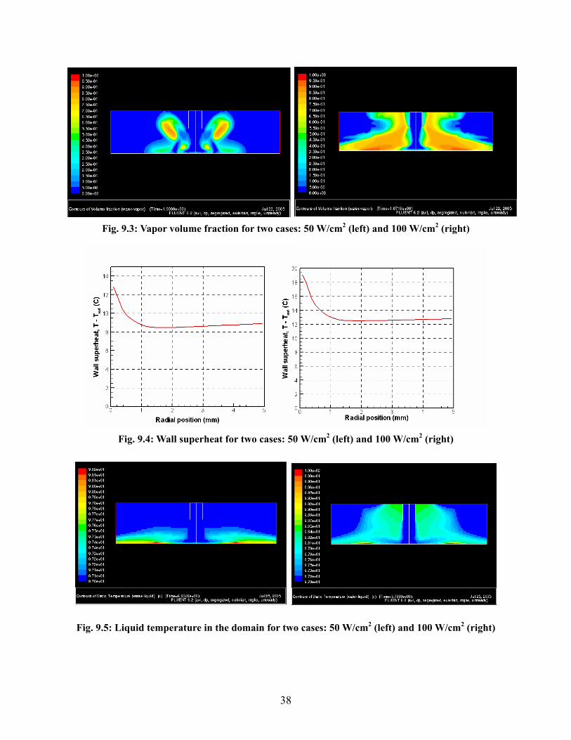
Fig. 9.3: Vapor volume fraction for two cases: 50 W/cm2 (left) and 100 W/cm2 (right)

Fig. 9.4: Wall superheat for two cases: 50 W/cm2 (left) and 100 W/cm2 (right)

Fig. 9.5: Liquid temperature in the domain for two cases: 50 W/cm2 (left) and 100 W/cm2 (right)

38

9.2 Impact of Jet Orientation

Typically, experiments have revealed that jet orientation does not affect nucleate boiling [14, 35]. To study the impact of jet orientation with respect to gravity, in Fig. 9.1 [33] the direction of gravity was reversed. In one case, the direction of vapor rise is against gravity (the baseline case), whereas in another case the direction of vapor rise is in line with gravity. The results are summarized in Table 9.2. For both cases (with 100 W/cm2), there is not much difference in the average wall superheat and the stagnation superheat, which is in line with experimental observations. However, for the case in which the vapor rise is in line with gravity, the vapor volume fraction increases because gravity causes the vapor to get locked up near the walls. The small difference in liquid temperature may also be related to this effect.

9.3 Impact of Nozzle Diameter

The Katto and Kunihiro study [33] indicates that the jet diameter does not have much impact on the boiling curve. Here, we test the code with this experimental observation. For the case of 100 W/cm2, three different nozzle diameters are used (Table 9.3). The 1.6 and 1.16 mm cases are comparable in terms of average wall superheat, liquid temperature, and vapor content. With the 1.6 mm nozzle, the velocity is 2 m/s; with the 1.16 mm nozzle, the velocity is 2.5 m/s; and with the 0.71 mm nozzle, the velocity is 2.4 m/s. For the 0.71 mm nozzle, the results are a little different. One possible reason is that for this smallest diameter nozzle, the ratio of target plate to nozzle diameter starts to become high, resulting in differences in the physics.

Table 9.2: Impact of gravity on the thermal predictions for the case of 100 W/cm2 (Katto and Kunihiro [33])

Vapor

rise direction against gravity

Vapor rise direction in line with gravity

Average wall superheat, K

12.5 12.6

Average liquid temperature, K

370.6 370.8

Average vapor content

0.33 0.5

Stagnation superheat, K

19 19

39

Table 9.3: Impact of nozzle diameter on the thermal predictions for the case of 100 W/cm2 (Katto and Kunihiro [33])

Nozzle diameter

1.6 mm 1.16 mm

0.71 mm

Average wall superheat, K

12.5 12.6 13.6

Average liquid temperature, K

370.6 370.5 370.9

Vapor content

0.3 0.3 0.4

9.4 Validation with Zhou and Ma [28] Experimental Study

In this section, we consider another experimental study with submerged boiling jets. This is the study by Zhou and Ma [28] with a submerged R-113 jet. The domain is shown in Fig. 9.6. As a simplification, the domain is assumed to be axisymmetric. The nozzle diameter is 1 mm. The target plate (constantan foil) area in the actual experiment is 5 mm x 5 mm, corresponding to a disk of radius 2.8 mm. The distance between the end of the nozzle and the target surface is 5 mm. In the experiments, the stagnation zone temperature is measured with a spatial resolution of about 0.2 mm. Figure 9.7 shows the results of the validation. The R-113 properties at atmospheric pressure are listed in Table 9.1. The fluid subcooling is 18.5°C, which means that the jet inlet temperature is 302.3 K. Two different jet velocities are presented: 0.41 and 11.36 m/s. The flow at 0.41 m/s is probably close to being laminar (Re ~ 2,000). At the elevated velocity, the saturation temperature of the fluid changes along the target wall; this aspect is accounted for in the code. For reference, in Fig. 9.7, the average wall superheat obtained from CFD is plotted along with the stagnation wall superheats. The match between experiments and CFD predictions is fair. Overall, these validations give some confidence in the Eulerian multiphase model implemented in FLUENT. Hence, we look at some IGBT package simulations involving boiling jets in the next section.

40

11.2 mm

5.6 mm

q5 mm

1 mm nozzle

Inlet

10 mm

Fig. 9.6: Domain for the Zhou and Ma [28] validation study

Fig. 9.7: Boiling curves from experiments and CFD predictions for the Zhou and Ma case [28] with

jet inlet velocities of 0.41 m/s and 11.36 m/s

41

10. IGBT Package Simulations with Boiling Jets

In the previous section, we established some confidence in the CFD predictions of FLUENT by comparison with experimental data from the literature. In this section, we explore IGBT package simulations with boiling jets. The axisymmetric domain used in the simulation is shown in Fig. 10.1. This domain is similar to the one presented in Section 4 with single-phase jets. The only difference is that in the domain here, the solder layer is considered as a wall with a certain thickness as opposed to explicitly being a separate layer in the domain. When the solder layer is a separate layer, it must be meshed. This poses problems because it implies a very thin layer must be meshed. These boiling simulations are fairly intensive and take several hours to converge, even with a small spatial mesh; for stability, they must be performed as transient simulations. If the spatial mesh is large, the simulations become quite intensive. Because of these factors, a fairly coarse mesh is used in the solid domain. In the liquid domain, the mesh is primarily governed by the need to keep the wall y+ above 11. The mesh used in the current simulations probably is mesh independent to about 10%.

These simulations are performed with water at 105°C. For the boiling simulations, the pressure is maintained at 1.35e+05 Pa, at which saturation temperature of the water is 108°C. So, there is a 3°C subcooling in the water temperature at the inlet. A volumetric heat generation term is included in the silicon layer to simulated heat dissipate. Two cases are considered – corresponding to 45 and 90 W/cm2 heat flux in the silicon die. These correspond to a heat dissipation of 36.5 and 73 W, respectively, in the silicon die. The jet inlet velocity is 2 m/s (Fig. 10.2). Figures 10.2 and 10.3 show the velocity and temperature contours, respectively, in the domain. For the case of 45 W/cm2, a maximum temperature of 121.5 °C is attained, while a maximum temperature of 139.3 °C is attained for the 90 W/cm2 case. The maximum temperatures are in the silicon die – as expected. The vapor volume fractions in the domain for the two cases are shown in Fig. 10.4. Clearly, the vapor generated for the 90 W/cm2 case is much larger than for the 45 W/cm2 case. The volume-averaged vapor fractions for the two cases are indicated in Table 10.2. For the 45 W/cm2 case, the volume-averaged vapor fraction is only 6%, while it is almost 70% for the 90 W/cm2. Figure 10.4 also gives a hint that in this reduced IGBT structure, the vapor does not have a very clear removal path. It tends to get trapped to some extent due to the confining copper and aluminum walls.

42

CopperAluminum

Fig. 10.1: Axisymmetric domain used for the IGBT package simulation

Fig. 10.2: Velocity contours in the domain

43

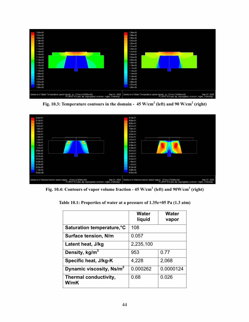
Fig. 10.3: Temperature contours in the domain - 45 W/cm2 (left) and 90 W/cm2 (right)

Fig. 10.4: Contours of vapor volume fraction - 45 W/cm2 (left) and 90W/cm2 (right)

Table 10.1: Properties of water at a pressure of 1.35e+05 Pa (1.3 atm)

Water

liquid Water vapor

Saturation temperature,°C 108

Surface tension, N/m 0.057

Latent heat, J/kg 2,235,100

Density, kg/m3 953 0.77

Specific heat, J/kg-K 4,228 2,068

Dynamic viscosity, Ns/m2 0.000262 0.0000124

Thermal conductivity, W/mK

0.68 0.026

44

In the past several sections, we have looked at single-phase jets and boiling jets. It would be useful to compare the performance of single-phase and boiling jets in the context of the IGBT package cooling. Figure 10.5 shows such a comparison for the case of 45 W/cm2. The plot on the left in Fig. 10.5 is the same as the plot on the left in Fig. 10.3, whereas the plot on the right in Fig. 10.5 is the case in which there is no boiling and everything else is identical to the case mentioned in this section. Figure 10.6 shows the case with and without boiling for 90 W/cm2. Table 10.2 also has a summary of all the results with and without boiling. For the cases not involving any boiling, the bubble nucleation site density is equal to zero. In all other aspects they are similar to the case involving boiling. This facilitates a direct comparison between the results from the two cases. The results are interesting. For the heat flux of 45 W/cm2, the case involving boiling gives maximum temperatures almost 2 degrees lower than the case not involving any boiling (Table 10.2). This translates to difference of about 10%. For the heat flux of 90 W/cm2, the case involving boiling actually yields maximum temperatures 2.7 degrees lower than the case not involving any boiling (Table 10.2). This translates to a difference of about 8 %. It is hard to conclusively state that boiling is giving any benefits over the case where there is no boiling – since the magnitude of enhancement is only about 10%. It is possible, that the mass fraction of the vapor being formed is not sufficient for boiling to be more beneficial than the single-phase jet impingement regime. The other possibility is that the geometry is preventing efficient removal of the vapor that is formed.

Fig. 10.5: Temperature contours in the domain with boiling (left) and without boiling (right) –

for 45 W/cm2

45

Fig. 10.6: Temperature contours in the domain with boiling (left) and without boiling (right) – for

90 W/cm2

Table 10.2: Summary of results obtained from IGBT package simulations

45 W/cm2 90 W/cm2

With boiling

Without boiling

With boiling

Without boiling

Tmax (°C) 121.5 123.4 139.3 142

Volume averaged vapor fraction

0.06 0 0.7 0

Volume averaged liquid temperature (°C)

105.2 105.2 106.3 105.4

Interestingly, what this means is that for this geometry and problem, from a heat transfer standpoint, forced convection cooling is almost as effective as the mechanism of vapor bubble nucleation in terms of thermal management of the silicon die. Of course, these numerical results need to be validated experimentally. The validations presented in section 9 give some degree of confidence in the predictions from the code. It would be interesting to see how experimental results from the IGBT package involving boiling would match up with the predictions presented here.

46

11. Summary and Conclusions

A survey of the nucleate jet impingement boiling literature indicates substantial experimental nucleate boiling data. There is considerable scatter in the data: uncertainties on the order of 40% are quite common. The nature of the target surface and the fluid-surface interaction is critical in determining the bubble nucleation process. The important CHF correlations in the literature yield results that agree with one another. Saturated fluorinerts (FC72, 77, 84) and OS-10 yield low CHFs on the order of 50 W/cm2, even with velocities as high as 8 m/s. Fluids such as water, ammonia, and R-134a have much superior heat transfer characteristics than fluorinerts. Several jet parameters—such as diameter, nozzle-to-target separation, velocity, number of jets, and orientation—do not have much of an impact on the nucleate boiling phenomenon.

We have observed some of these effects in our CFD simulations also. The CFD model and code are validated against two experimental studies involving submerged jets. To the best of our knowledge, this is the first time such validations are being reported. A reasonable match is found between the experimental boiling curves and those obtained by CFD. IGBT package simulations suggest that for the limited number of cases examined here, boiling jets are not providing any significant benefits over non-boiling jets. It is not entirely clear under what conditions boiling jets would be more beneficial than single-phase jets in the context of IGBT package cooling.

Regarding practical implementation with boiling jets, a separate loop would be necessary. Water is eliminated from the picture owing to freezing problems. Similar problems eliminate having boiling with the glycol-water mixture. Perhaps R-134a could be used, but this must be investigated further.

Overall, it appears the single-phase glycol-water jets in the single-phase regime should be investigated further. Glycol-water is likely to be readily accepted as a working fluid by the automotive industry. If practical concerns relating to reliability, erosion, corrosion, and package stresses are addressed, glycol-water jets can be implemented realistically. With further heat transfer enhancements, they can remove high heat fluxes of up to 200 W/cm2. In this first part of the report, we have demonstrated baseline conditions under which it may be possible to dissipate such heat fluxes using glycol-water jets in the single-phase regime.

Acknowledgments We acknowledge the support and funding provided by Susan Rogers, the program manager

for the advanced power electronics and electric machines project under DOE’s FreedomCAR Program. The numerical simulations on boiling jets were carried out in close collaboration with Andrey Troshko at Fluent, Inc. The material presented in Appendix B was also provided by Andrey Troshko.

47

Appendix A: Properties of Various Fluids (from Aspen) FC-87 Mol. Wt 288TEMP LIQUID VAPOR LIQUID VAPOR LIQUID VAPOR LIQUID VAPOR LIQUID LIQUID VAPOR TOTAL LIQUID VAPOR H-fg DENSITY DENSITY SPECIFIC SPECIFIC DYNAMIC DYNAMIC THERMAL THERMAL SURFACE PR PR PRES ENTHALPYENTHALPY HEAT HEAT VISCOSITYVISCOSITYCOND. COND. TENSION C kg/cum kg/cum kJ/kg-K kJ/kg-K N-sec/sqm N-sec/sqm Watt/m-K Watt/m-K N/m bar kJ/kg kJ/kg

-40 2169.412 0.440451 0.813851 0.614201 0.000521 9.24E-06 0.082135 0.006751 0.016385 5.159073 0.840185 0.029552 -9352.764 -9244.76 108.004-30 2132.848 0.816272 0.846947 0.646248 0.000467 9.58E-06 0.079699 0.007348 0.015409 4.960655 0.842347 0.056989 -9344.46 -9238.509 105.951-20 2095.454 1.426084 0.881347 0.679103 0.000422 9.92E-06 0.077263 0.007978 0.014433 4.815456 0.844777 0.103313 -9335.818 -9231.963 103.855-10 2057.148 2.367658 0.917106 0.712805 0.000385 1.03E-05 0.074827 0.00864 0.013457 4.714859 0.847611 0.177453 -9326.824 -9225.126 101.698

0 2017.836 3.76159 0.954304 0.747406 0.000353 1.06E-05 0.072392 0.009335 0.01248 4.652751 0.851002 0.290731 -9317.465 -9218.004 99.46110 1977.407 5.753317 0.987527 0.777447 0.000326 1.10E-05 0.069956 0.009995 0.011504 4.599171 0.854992 0.456967 -9307.734 -9210.612 97.12220 1935.728 8.516112 1.009805 0.79589 0.000302 1.14E-05 0.06752 0.010521 0.010528 4.522448 0.859702 0.692499 -9297.742 -9203.088 94.65430 1892.638 12.25584 1.033056 0.814555 0.000282 1.17E-05 0.065084 0.011053 0.009552 4.4768 0.86576 1.016151 -9287.523 -9195.492 92.03140 1847.942 17.21839 1.057598 0.833619 0.000262 1.21E-05 0.062483 0.011592 0.008585 4.428371 0.873543 1.449147 -9277.064 -9187.848 89.21650 1801.394 23.70943 1.083873 0.853332 0.000239 1.26E-05 0.059637 0.012137 0.007638 4.348479 0.883568 2.015641 -9266.354 -9180.181 86.17360 1752.684 32.09211 1.112519 0.874044 0.000216 1.30E-05 0.056647 0.012688 0.006711 4.244561 0.896535 2.741022 -9255.374 -9172.521 82.85370 1701.404 42.84063 1.144486 0.896294 0.000193 1.35E-05 0.053568 0.013245 0.005808 4.126203 0.913491 3.653775 -9244.103 -9164.901 79.20280 1647.01 56.57427 1.181256 0.92094 0.000171 1.40E-05 0.050417 0.013806 0.004929 4.005784 0.936038 4.784462 -9232.509 -9157.364 75.14590 1588.74 74.13904 1.225277 0.949438 0.00015 1.46E-05 0.047167 0.014372 0.004078 3.899832 0.966795 6.165969 -9220.549 -9149.963 70.586

100 1525.471 96.7471 1.280911 0.984471 0.000131 1.53E-05 0.043748 0.014943 0.003258 3.832127 1.010382 7.833454 -9208.162 -9142.77 65.392110 1455.44 126.3138 1.35677 1.031635 0.000113 1.62E-05 0.040051 0.015518 0.002474 3.841641 1.076055 9.827491 -9195.252 -9135.895 59.357120 1375.579 165.9498 1.472791 1.104262 9.77E-05 1.73E-05 0.035924 0.016096 0.001734 4.006811 1.184912 12.18665 -9181.659 -9129.503 52.156130 1279.627 221.8071 1.688304 1.244232 8.38E-05 1.88E-05 0.031171 0.016679 0.001048 4.540739 1.401041 14.95558 -9167.07 -9123.914 43.156

FC-72 Mol. Wt 338TEMP LIQUID VAPOR LIQUID VAPOR LIQUID VAPOR LIQUID VAPOR LIQUID LIQUID VAPOR TOTAL LIQUID VAPOR Hfg DENSITY DENSITY SPECIFIC SPECIFIC DYNAMIC DYNAMIC THERMAL THERMAL SURFACE PR PR PRES ENTHALPY ENTHALPY HEAT HEAT VISC. VISC. COND. COND. TENSION C kg/cum kg/cum kJ/kg-K kJ/kg-K N-sec/sqm N-sec/sqm Watt/m-K Watt/m-K N/m bar kJ/kg kJ/kg

-40 2612.37 0.028214 0.860321 0.612126 0.000766 8.58E-06 0.081051 6.23E-03 0.016882 8.13169 0.843564 0.001617 -9237.666 -9110.258 127.408-30 2570.31 0.066921 0.892533 0.64503 0.000678 8.90E-06 0.078867 6.80E-03 0.016022 7.674133 0.844932 0.004 -9228.903 -9103.979 124.924-20 2527.496 0.145709 0.925991 0.678649 0.000606 9.22E-06 0.076682 7.40E-03 0.015162 7.31839 0.84627 0.009062 -9219.811 -9097.373 122.438-10 2483.866 0.294413 0.960707 0.71299 0.000546 9.55E-06 0.074497 8.03E-03 0.014301 7.044734 0.847629 0.019013 -9210.378 -9090.438 119.94

0 2439.348 0.557218 0.996707 0.74807 0.000496 9.87E-06 0.072313 8.69E-03 0.013441 6.838821 0.849074 0.037289 -9200.592 -9083.172 117.4210 2393.858 0.995901 1.028204 0.778082 0.000454 1.02E-05 0.070128 9.32E-03 0.012581 6.652442 0.850542 0.068905 -9190.447 -9075.585 114.86220 2347.302 1.692838 1.047765 0.795566 0.000417 1.05E-05 0.067944 9.82E-03 0.011721 6.437611 0.851998 0.120796 -9180.066 -9067.816 112.2530 2299.567 2.753875 1.067837 0.81293 0.000386 1.08E-05 0.065759 1.03E-02 0.010861 6.271358 0.853899 0.202114 -9169.486 -9059.922 109.56440 2250.521 4.311383 1.088563 0.830254 0.000359 1.12E-05 0.063574 1.08E-02 0.010001 6.148139 0.856395 0.324457 -9158.702 -9051.92 106.78250 2200.008 6.528043 1.110129 0.847643 0.000335 1.15E-05 0.06139 1.14E-02 0.009141 6.064135 0.859674 0.50204 -9147.705 -9043.829 103.87660 2147.837 9.602192 1.132791 0.86523 0.000314 1.19E-05 0.059181 1.19E-02 0.008282 6.008568 0.86397 0.751795 -9136.487 -9035.672 100.81570 2093.774 13.7758 1.156895 0.883193 0.00029 1.22E-05 0.056757 1.24E-02 0.007436 5.905558 0.869583 1.093418 -9125.036 -9027.473 97.56380 2037.53 19.34659 1.182929 0.901781 0.000263 1.26E-05 0.054159 1.29E-02 0.006608 5.746804 0.876919 1.549389 -9113.336 -9019.259 94.07790 1978.732 26.69589 1.211594 0.921357 0.000236 1.30E-05 0.051456 1.35E-02 0.005798 5.546299 0.886557 2.14562 -9101.368 -9011.064 90.304

100 1916.896 36.29747 1.243941 0.942463 0.000208 1.34E-05 0.048684 1.40E-02 0.005008 5.320613 0.899323 2.909905 -9089.107 -9002.925 86.182110 1851.366 48.79144 1.281615 0.965982 0.000182 1.38E-05 0.045845 1.46E-02 0.00424 5.089172 0.916518 3.873778 -9076.517 -8994.889 81.628120 1781.224 65.05641 1.327349 0.993425 0.000158 1.43E-05 0.042905 1.51E-02 0.003497 4.875431 0.940294 5.071724 -9063.549 -8987.017 76.532130 1705.112 86.36403 1.386054 1.027613 0.000135 1.49E-05 0.039798 1.57E-02 0.002781 4.710197 0.974516 6.541475 -9050.132 -8979.391 70.741

48

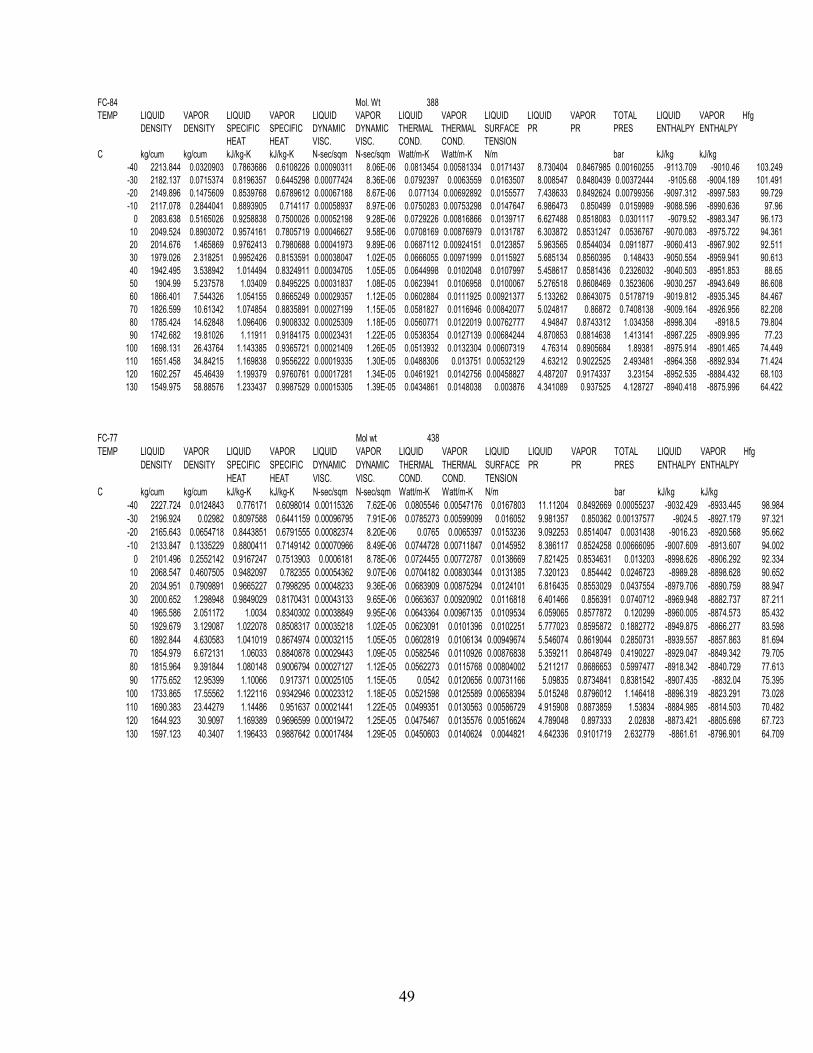
FC-84 Mol. Wt 388TEMP LIQUID VAPOR LIQUID VAPOR LIQUID VAPOR LIQUID VAPOR LIQUID LIQUID VAPOR TOTAL LIQUID VAPOR Hfg DENSITY DENSITY SPECIFIC SPECIFIC DYNAMIC DYNAMIC THERMAL THERMAL SURFACE PR PR PRES ENTHALPY ENTHALPY HEAT HEAT VISC. VISC. COND. COND. TENSION C kg/cum kg/cum kJ/kg-K kJ/kg-K N-sec/sqm N-sec/sqm Watt/m-K Watt/m-K N/m bar kJ/kg kJ/kg

-40 2213.844 0.0320903 0.7863686 0.6108226 0.00090311 8.06E-06 0.0813454 0.00581334 0.0171437 8.730404 0.8467985 0.00160255 -9113.709 -9010.46 103.249-30 2182.137 0.0715374 0.8196357 0.6445298 0.00077424 8.36E-06 0.0792397 0.0063559 0.0163507 8.008547 0.8480439 0.00372444 -9105.68 -9004.189 101.491-20 2149.896 0.1475609 0.8539768 0.6789612 0.00067188 8.67E-06 0.077134 0.00692892 0.0155577 7.438633 0.8492624 0.00799356 -9097.312 -8997.583 99.729-10 2117.078 0.2844041 0.8893905 0.714117 0.00058937 8.97E-06 0.0750283 0.00753298 0.0147647 6.986473 0.850499 0.0159989 -9088.596 -8990.636 97.96

0 2083.638 0.5165026 0.9258838 0.7500026 0.00052198 9.28E-06 0.0729226 0.00816866 0.0139717 6.627488 0.8518083 0.0301117 -9079.52 -8983.347 96.17310 2049.524 0.8903072 0.9574161 0.7805719 0.00046627 9.58E-06 0.0708169 0.00876979 0.0131787 6.303872 0.8531247 0.0536767 -9070.083 -8975.722 94.36120 2014.676 1.465869 0.9762413 0.7980688 0.00041973 9.89E-06 0.0687112 0.00924151 0.0123857 5.963565 0.8544034 0.0911877 -9060.413 -8967.902 92.51130 1979.026 2.318251 0.9952426 0.8153591 0.00038047 1.02E-05 0.0666055 0.00971999 0.0115927 5.685134 0.8560395 0.148433 -9050.554 -8959.941 90.61340 1942.495 3.538942 1.014494 0.8324911 0.00034705 1.05E-05 0.0644998 0.0102048 0.0107997 5.458617 0.8581436 0.2326032 -9040.503 -8951.853 88.6550 1904.99 5.237578 1.03409 0.8495225 0.00031837 1.08E-05 0.0623941 0.0106958 0.0100067 5.276518 0.8608469 0.3523606 -9030.257 -8943.649 86.60860 1866.401 7.544326 1.054155 0.8665249 0.00029357 1.12E-05 0.0602884 0.0111925 0.00921377 5.133262 0.8643075 0.5178719 -9019.812 -8935.345 84.46770 1826.599 10.61342 1.074854 0.8835891 0.00027199 1.15E-05 0.0581827 0.0116946 0.00842077 5.024817 0.86872 0.7408138 -9009.164 -8926.956 82.20880 1785.424 14.62848 1.096406 0.9008332 0.00025309 1.18E-05 0.0560771 0.0122019 0.00762777 4.94847 0.8743312 1.034358 -8998.304 -8918.5 79.80490 1742.682 19.81026 1.11911 0.9184175 0.00023431 1.22E-05 0.0538354 0.0127139 0.00684244 4.870853 0.8814638 1.413141 -8987.225 -8909.995 77.23

100 1698.131 26.43764 1.143385 0.9365721 0.00021409 1.26E-05 0.0513932 0.0132304 0.00607319 4.76314 0.8905684 1.89381 -8975.914 -8901.465 74.449110 1651.458 34.84215 1.169838 0.9556222 0.00019335 1.30E-05 0.0488306 0.013751 0.00532129 4.63212 0.9022525 2.493481 -8964.358 -8892.934 71.424120 1602.257 45.46439 1.199379 0.9760761 0.00017281 1.34E-05 0.0461921 0.0142756 0.00458827 4.487207 0.9174337 3.23154 -8952.535 -8884.432 68.103130 1549.975 58.88576 1.233437 0.9987529 0.00015305 1.39E-05 0.0434861 0.0148038 0.003876 4.341089 0.937525 4.128727 -8940.418 -8875.996 64.422

FC-77 Mol wt 438TEMP LIQUID VAPOR LIQUID VAPOR LIQUID VAPOR LIQUID VAPOR LIQUID LIQUID VAPOR TOTAL LIQUID VAPOR Hfg DENSITY DENSITY SPECIFIC SPECIFIC DYNAMIC DYNAMIC THERMAL THERMAL SURFACE PR PR PRES ENTHALPY ENTHALPY HEAT HEAT VISC. VISC. COND. COND. TENSION C kg/cum kg/cum kJ/kg-K kJ/kg-K N-sec/sqm N-sec/sqm Watt/m-K Watt/m-K N/m bar kJ/kg kJ/kg

-40 2227.724 0.0124843 0.776171 0.6098014 0.00115326 7.62E-06 0.0805546 0.00547176 0.0167803 11.11204 0.8492669 0.00055237 -9032.429 -8933.445 98.98-30 2196.924 0.02982 0.8097588 0.6441159 0.00096795 7.91E-06 0.0785273 0.00599099 0.016052 9.981357 0.850362 0.00137577 -9024.5 -8927.179 97.321-20 2165.643 0.0654718 0.8443851 0.6791555 0.00082374 8.20E-06 0.0765 0.0065397 0.0153236 9.092253 0.8514047 0.0031438 -9016.23 -8920.568 95.662-10 2133.847 0.1335229 0.8800411 0.7149142 0.00070966 8.49E-06 0.0744728 0.00711847 0.0145952 8.386117 0.8524258 0.00666095 -9007.609 -8913.607 94.002

0 2101.496 0.2552142 0.9167247 0.7513903 0.0006181 8.78E-06 0.0724455 0.00772787 0.0138669 7.821425 0.8534631 0.013203 -8998.626 -8906.292 92.33410 2068.547 0.4607505 0.9482097 0.782355 0.00054362 9.07E-06 0.0704182 0.00830344 0.0131385 7.320123 0.854442 0.0246723 -8989.28 -8898.628 90.65220 2034.951 0.7909891 0.9665227 0.7998295 0.00048233 9.36E-06 0.0683909 0.00875294 0.0124101 6.816435 0.8553029 0.0437554 -8979.706 -8890.759 88.94730 2000.652 1.298948 0.9849029 0.8170431 0.00043133 9.65E-06 0.0663637 0.00920902 0.0116818 6.401466 0.856391 0.0740712 -8969.948 -8882.737 87.21140 1965.586 2.051172 1.0034 0.8340302 0.00038849 9.95E-06 0.0643364 0.00967135 0.0109534 6.059065 0.8577872 0.120299 -8960.005 -8874.573 85.43250 1929.679 3.129087 1.022078 0.8508317 0.00035218 1.02E-05 0.0623091 0.0101396 0.0102251 5.777023 0.8595872 0.1882772 -8949.875 -8866.277 83.59860 1892.844 4.630583 1.041019 0.8674974 0.00032115 1.05E-05 0.0602819 0.0106134 0.00949674 5.546074 0.8619044 0.2850731 -8939.557 -8857.863 81.69470 1854.979 6.672131 1.06033 0.8840878 0.00029443 1.09E-05 0.0582546 0.0110926 0.00876838 5.359211 0.8648749 0.4190227 -8929.047 -8849.342 79.70580 1815.964 9.391844 1.080148 0.9006794 0.00027127 1.12E-05 0.0562273 0.0115768 0.00804002 5.211217 0.8686653 0.5997477 -8918.342 -8840.729 77.61390 1775.652 12.95399 1.10066 0.917371 0.00025105 1.15E-05 0.0542 0.0120656 0.00731166 5.09835 0.8734841 0.8381542 -8907.435 -8832.04 75.395

100 1733.865 17.55562 1.122116 0.9342946 0.00023312 1.18E-05 0.0521598 0.0125589 0.00658394 5.015248 0.8796012 1.146418 -8896.319 -8823.291 73.028110 1690.383 23.44279 1.14486 0.951637 0.00021441 1.22E-05 0.0499351 0.0130563 0.00586729 4.915908 0.8873859 1.53834 -8884.985 -8814.503 70.482120 1644.923 30.9097 1.169389 0.9696599 0.00019472 1.25E-05 0.0475467 0.0135576 0.00516624 4.789048 0.897333 2.02838 -8873.421 -8805.698 67.723130 1597.123 40.3407 1.196433 0.9887642 0.00017484 1.29E-05 0.0450603 0.0140624 0.0044821 4.642336 0.9101719 2.632779 -8861.61 -8796.901 64.709

4

49

OS-10 C6H18OSI2 HEXAMETHYLDISILOXANE Mol wt 138TEMP LIQUID VAPOR LIQUID VAPOR LIQUID VAPOR LIQUID VAPOR LIQUID LIQUID VAPOR TOTAL LIQUID VAPOR Hfg DENSITY DENSITY SPECIFIC SPECIFIC DYNAMIC DYNAMIC THERMAL THERMAL SURFACE PR PR PRES ENTHALPY ENTHALPY HEAT HEAT VISC. VISC. COND. COND. TENSION C kg/cum kg/cum kJ/kg-K kJ/kg-K N-sec/sqm N-sec/sqm Watt/m-K Watt/m-K N/m bar kJ/kg kJ/kg

-40 822.5764 0.00665639 1.63297 1.298418 0.00126701 5.12E-06 0.1488421 0.00732088 0.0213692 13.90052 0.9081757 0.00079451 -5123.997 -4879.131 244.866-30 813.3439 0.0147589 1.653871 1.320679 0.00105816 5.37E-06 0.1457652 0.00805451 0.0204219 12.00605 0.879904 0.00183689 -5107.564 -4866.043 241.521-20 803.9766 0.0303654 1.677041 1.344633 0.00089552 5.61E-06 0.1426883 0.00878813 0.0194839 10.52524 0.8585539 0.00393353 -5090.911 -4852.729 238.182-10 794.4662 0.0585073 1.702261 1.370077 0.00076685 5.86E-06 0.1396114 0.00952176 0.0185554 9.350144 0.8425326 0.00787441 -5074.016 -4839.177 234.839

0 784.8034 0.1064049 1.729318 1.396806 0.00066361 6.10E-06 0.1365345 0.0102553 0.0176368 8.405163 0.8306901 0.014853 -5056.859 -4825.378 231.48110 774.978 0.1838986 1.758009 1.424625 0.0005797 6.34E-06 0.1334576 0.010989 0.0167283 7.636355 0.8221779 0.0265778 -5039.423 -4811.327 228.09620 764.9788 0.3038214 1.788151 1.453353 0.00051072 6.58E-06 0.1303807 0.0117226 0.0158302 7.004555 0.8163609 0.04538 -5021.691 -4797.023 224.66830 754.793 0.4823007 1.819586 1.48283 0.00045342 6.83E-06 0.1273038 0.0124562 0.0149429 6.480888 0.8127606 0.0743122 -5003.651 -4782.467 221.18440 744.4063 0.7389978 1.852186 1.512917 0.00040535 7.07E-06 0.1242269 0.0131899 0.0140667 6.043778 0.8110165 0.117229 -4985.29 -4767.665 217.62550 733.8028 1.097315 1.885856 1.543504 0.00036469 7.31E-06 0.12115 0.0139235 0.013202 5.676905 0.8108603 0.1788457 -4966.596 -4752.627 213.96960 722.9641 1.58461 1.920542 1.574508 0.00033 7.56E-06 0.1180731 0.0146571 0.0123493 5.36781 0.812098 0.2647765 -4947.558 -4737.365 210.19370 711.8693 2.232483 1.956232 1.605875 0.0003002 7.81E-06 0.1149962 0.0153907 0.011509 5.106899 0.8145975 0.3815502 -4928.167 -4721.894 206.27380 700.4945 3.077183 1.992965 1.637586 0.00027442 8.06E-06 0.1119193 0.0161244 0.0106817 4.886757 0.8182815 0.5366084 -4908.412 -4706.232 202.1890 688.8116 4.160226 2.030835 1.66966 0.00025198 8.31E-06 0.1088424 0.016858 0.00986782 4.701646 0.8231234 0.7382907 -4888.283 -4690.398 197.885

100 676.7879 5.529292 2.070008 1.702158 0.00023233 8.57E-06 0.1057655 0.0175916 0.00906805 4.547155 0.8291474 0.9958106 -4867.769 -4674.417 193.352110 664.3848 7.239511 2.110737 1.735195 0.00021507 8.83E-06 0.1026886 0.0183288 0.0082831 4.420789 0.8362712 1.319225 -4846.855 -4658.314 188.541120 651.5557 9.355248 2.153386 1.768952 0.00019988 9.11E-06 0.0996116 0.0190737 0.00751376 4.320965 0.8444679 1.719395 -4825.527 -4642.118 183.409130 638.2443 11.95623 2.198472 1.803715 0.00018643 9.39E-06 0.0965347 0.019826 0.00676092 4.245864 0.8540099 2.208536 -4803.767 -4625.862 177.905

R134a C2H2F4 1,1,1,2-TETRAFLUOROETHANE Mol wt 102TEMP LIQUID VAPOR LIQUID VAPOR LIQUID VAPOR LIQUID VAPOR LIQUID LIQUID VAPOR TOTAL LIQUID VAPOR Hfg DENSITY DENSITY SPECIFIC SPECIFIC DYNAMIC DYNAMIC THERMAL THERMAL SURFACE PR PR PRES ENTHALPY ENTHALPY HEAT HEAT VISC. VISC. COND. COND. TENSION C kg/cum kg/cum kJ/kg-K kJ/kg-K N-sec/sqm N-sec/sqm Watt/m-K Watt/m-K N/m bar kJ/kg kJ/kg

-40 237.2421 0.4611456 7.113574 4.304863 0.0004582 9.24E-06 0.1118832 0.00877817 0.017549 29.13264 4.533588 0.514659 -54256.99 -52906.23 1350.76-30 232.2614 0.7326537 7.29484 4.437051 0.00040261 9.67E-06 0.107296 0.0094317 0.0160074 27.3732 4.5487 0.8446854 -54184.89 -52866.35 1318.54-20 227.1148 1.117957 7.49628 4.578949 0.00035405 1.01E-05 0.1027119 0.0100876 0.0144949 25.84012 4.581897 1.325307 -54110.85 -52826.62 1284.23-10 221.7793 1.648871 7.721196 4.732229 0.00031167 1.05E-05 0.098131 0.0107551 0.0130134 24.52341 4.629173 1.999861 -54034.67 -52787.33 1247.34

0 216.2268 2.364012 7.974679 4.899621 0.00027471 1.10E-05 0.0935533 0.0114349 0.011565 23.41722 4.692356 2.91761 -53956.1 -52748.82 1207.2810 210.4211 3.309706 8.264485 5.085336 0.00024247 1.14E-05 0.0889787 0.0121262 0.0101521 22.52169 4.77524 4.132022 -53874.84 -52711.45 1163.3920 204.3156 4.544748 8.602534 5.296129 0.00021434 1.18E-05 0.0844073 0.0128286 0.00877755 21.8458 4.884087 5.70205 -53790.55 -52675.68 1114.8730 197.8477 6.145251 9.00768 5.543016 0.00018978 1.23E-05 0.0798391 0.0135417 0.00744487 21.41236 5.029215 7.691183 -53702.75 -52642.09 1060.6640 190.9306 8.214045 9.511156 5.844856 0.00016831 1.28E-05 0.075274 0.0142649 0.00615844 21.26768 5.228328 10.16753 -53610.84 -52611.37 999.4750 183.4377 10.89695 10.16834 6.236217 0.00014953 1.33E-05 0.0707121 0.014998 0.00492388 21.50242 5.513844 13.20368 -53513.93 -52584.48 929.4560 175.1719 14.41975 11.08716 6.78798 0.00013306 1.38E-05 0.0661534 0.0157404 0.00374873 22.30192 5.95217 16.881 -53410.74 -52562.87 847.8770 165.7964 19.14706 12.51127 7.665124 0.00011862 1.44E-05 0.0615978 0.0164918 0.00264369 24.09349 6.697656 21.27995 -53299.12 -52548.72 750.480 154.6429 25.77939 15.13409 9.361812 0.00010617 1.51E-05 0.0570454 0.0172518 0.00162554 28.16858 8.213877 26.49102 -53175.06 -52546.11 628.9590 139.9615 36.05353 22.07586 14.26121 9.56E-05 1.61E-05 0.052496 0.0180201 0.00072545 40.2103 12.7564 32.61774 -53028.82 -52564.98 463.84

100 114.5738 58.83925 195.7743 99.10105 8.66E-05 1.82E-05 0.0479473 0.0187963 3.74E-05 353.5831 95.98024 39.72892 -52798.99 -52654.56 144.43

50

Water H2O Mol wt 18TEMP LIQUID VAPOR LIQUID VAPOR LIQUID VAPOR LIQUID VAPOR LIQUID LIQUID VAPOR TOTAL LIQUID VAPOR Hfg DENSITY DENSITY SPECIFIC SPECIFIC DYNAMIC DYNAMIC THERMAL THERMAL SURFACE PR PR PRES ENTHALPY ENTHALPY HEAT HEAT VISC. VISC. COND. COND. TENSION C kg/cum kg/cum kJ/kg-K kJ/kg-K N-sec/sqm N-sec/sqm Watt/m-K Watt/m-K N/m bar kJ/kg kJ/kg

-40 996.436 0.00026529 4.208358 1.85412 0.0174547 8.57E-06 0.5358424 0.0155843 0 137.0848 1.020093 0.00033442 -16138.67 -13543.26 2595.41-30 997.2833 0.00054849 4.209211 1.854973 0.00783347 8.66E-06 0.5253507 0.0158188 0 62.76326 1.015991 0.0006914 -16096.58 -13524.73 2571.85-20 998.1321 0.00113418 4.210273 1.856035 0.00425691 8.81E-06 0.5298711 0.0161575 0 33.8247 1.011948 0.00142962 -16054.48 -13506.2 2548.28-10 998.9823 0.0023455 4.211564 1.857326 0.00263733 9.00E-06 0.5428722 0.0165789 0 20.46021 1.007852 0.00295618 -16012.37 -13487.69 2524.68

0 999.7834 0.00484272 4.213165 1.850891 0.00179306 9.22E-06 0.5604835 0.0170696 0 13.47846 0.9992648 0.00610234 -15970.35 -13469.23 2501.1210 999.7544 0.00939079 4.18802 1.855403 0.00130652 9.46E-06 0.5795539 0.01762 0.0742191 9.441265 0.9962152 0.0122631 -15928.36 -13450.92 2477.4420 998.2859 0.0172845 4.176913 1.861333 0.00100204 9.73E-06 0.5979781 0.0182259 0.0727341 6.999293 0.9933401 0.0233586 -15886.54 -13432.68 2453.8630 995.7174 0.0303648 4.173026 1.869128 0.00079768 1.00E-05 0.614995 0.018885 0.071192 5.412665 0.9907071 0.0424095 -15844.8 -13414.56 2430.2440 992.257 0.0511614 4.172934 1.879292 0.00065324 1.03E-05 0.6300836 0.0195969 0.069594 4.326306 0.9884052 0.07375 -15803.07 -13396.61 2406.4650 988.0378 0.0830177 4.175038 1.89162 0.00054704 1.06E-05 0.6430042 0.0203627 0.0679414 3.551943 0.9861498 0.1233641 -15761.33 -13378.86 2382.4760 983.1517 0.1302341 4.178751 1.907041 0.00046651 1.09E-05 0.6537398 0.0211847 0.0662356 2.982022 0.9842589 0.1992349 -15719.56 -13361.39 2358.1770 977.6682 0.1981679 4.184023 1.926046 0.00040395 1.13E-05 0.6624192 0.0220655 0.064478 2.551466 0.9828266 0.3116902 -15677.75 -13344.24 2333.5180 971.6428 0.293336 4.191068 1.949195 0.00035435 1.16E-05 0.6692465 0.0230084 0.0626699 2.219071 0.981996 0.4737259 -15635.88 -13327.47 2308.4190 965.119 0.4234995 4.200195 1.976979 0.00031436 1.19E-05 0.6744478 0.0240167 0.0608129 1.957753 0.9818894 0.7013016 -15593.92 -13311.15 2282.77

100 958.1296 0.5977343 4.211722 2.00999 0.00028167 1.23E-05 0.6782375 0.0250936 0.0589086 1.749138 0.9826914 1.013585 -15551.87 -13295.34 2256.53110 950.6984 0.8264961 4.225923 2.048955 0.0002546 1.26E-05 0.6807996 0.0262418 0.0569585 1.580418 0.9846598 1.433146 -15509.68 -13280.11 2229.57120 942.8411 1.121684 4.243019 2.094816 0.00023194 1.30E-05 0.6822817 0.027464 0.0549645 1.44246 0.9881528 1.986096 -15467.34 -13265.51 2201.83130 934.5673 1.496712 4.263191 2.148813 0.00021279 1.33E-05 0.6827945 0.0287622 0.0529284 1.328618 0.99365 2.702174 -15424.81 -13251.62 2173.19

Freon 113 C2CL3F3 Mol wt 176TEMP LIQUID VAPOR LIQUID VAPOR LIQUID VAPOR LIQUID VAPOR LIQUID LIQUID VAPOR TOTAL LIQUID VAPOR Hfg DENSITY DENSITY SPECIFIC SPECIFIC DYNAMIC DYNAMIC THERMAL THERMAL SURFACE PR PR PRES ENTHALPY ENTHALPY HEAT HEAT VISC. VISC. COND. COND. TENSION C kg/cum kg/cum kJ/kg-K kJ/kg-K N-sec/sqm N-sec/sqm Watt/m-K Watt/m-K N/m bar kJ/kg kJ/kg

-40 155.2175 0.0142899 9.053397 6.748997 0.00200901 8.10E-06 0.0878792 0.00493634 0.0246975 206.9703 11.07988 0.0162432 -46846.36 -45045.69 1800.67-30 153.3161 0.0262135 9.166337 6.856888 0.00162298 8.49E-06 0.0857565 0.00537421 0.023503 173.4764 10.8305 0.0310439 -46755.26 -44978 1777.26-20 151.3826 0.0454639 9.286305 6.967504 0.00133465 8.87E-06 0.0836338 0.00581279 0.0223192 148.1931 10.63547 0.055973 -46662.99 -44909.43 1753.56-10 149.4148 0.0750873 9.41261 7.080246 0.00111502 9.26E-06 0.0815111 0.00626228 0.0211473 128.7582 10.46592 0.0958909 -46569.48 -44840.03 1729.45

0 147.41 0.1188192 9.544778 7.194684 0.00094468 9.64E-06 0.0793884 0.00672579 0.0199876 113.5787 10.31257 0.1570419 -46474.67 -44769.88 1704.7910 145.3654 0.1811035 9.682565 7.310556 0.00081045 1.00E-05 0.0772657 0.00720304 0.0188406 101.5619 10.17359 0.2471511 -46378.5 -44699.08 1679.4220 143.2778 0.2671065 9.825972 7.427773 0.00070312 1.04E-05 0.075143 0.00769376 0.0177068 91.94293 10.04762 0.3754731 -46280.91 -44627.75 1653.1630 141.1437 0.3827374 9.975263 7.546417 0.00061618 1.08E-05 0.0730203 0.00819769 0.0165866 84.17616 9.933748 0.552794 -46181.84 -44556.02 1625.8240 138.9587 0.5346896 10.131 7.66676 0.00054491 1.12E-05 0.0708976 0.00871458 0.0154807 77.86645 9.831461 0.7913976 -46081.23 -44484.04 1597.1950 136.7181 0.7305143 10.29407 7.789276 0.00048587 1.16E-05 0.0687749 0.00924417 0.0143896 72.72396 9.74061 1.105003 -45979.01 -44411.98 1567.0360 134.4164 0.9787418 10.46579 7.914687 0.00043646 1.19E-05 0.0666522 0.00978623 0.0133141 68.53436 9.661429 1.508686 -45875.1 -44340.01 1535.0970 132.0468 1.289064 10.64795 8.044016 0.00039475 1.23E-05 0.0645295 0.0103405 0.012255 65.13865 9.594574 2.018791 -45769.42 -44268.31 1501.1180 129.6017 1.672594 10.84303 8.178677 0.00035925 1.27E-05 0.0624068 0.0109068 0.011213 62.41975 9.5412 2.652839 -45661.85 -44197.11 1464.7490 127.0718 2.142725 11.05436 8.320679 0.0003288 1.31E-05 0.0602841 0.0114848 0.0101891 60.29345 9.503189 3.430129 -45552.27 -44126.64 1425.63

100 124.4455 2.714323 11.28653 8.472681 0.0003025 1.35E-05 0.0581614 0.0120744 0.00918462 58.70303 9.483128 4.36972 -45440.53 -44057.13 1383.4110 121.7089 3.406114 11.54587 8.638551 0.00027964 1.39E-05 0.0560387 0.0126754 0.00820059 57.61656 9.484987 5.492711 -45326.43 -43988.89 1337.54120 118.8443 4.240955 11.84142 8.823857 0.00025964 1.43E-05 0.053916 0.0132875 0.0072386 57.02509 9.514587 6.820953 -45209.74 -43922.25 1287.49130 115.8287 5.247725 12.18643 9.036939 0.00024197 1.47E-05 0.0517933 0.0139106 0.00630043 56.93502 9.580732 8.377307 -45090.15 -43857.62 1232.53

51

NH3 Mol wt 17TEMP LIQUID VAPOR LIQUID VAPOR LIQUID VAPOR LIQUID VAPOR LIQUID LIQUID VAPOR TOTAL LIQUID VAPOR Hfg DENSITY DENSITY SPECIFIC SPECIFIC DYNAMIC DYNAMIC THERMAL THERMAL SURFACE PR PR PRES ENTHALPY ENTHALPY HEAT HEAT VISC. VISC. COND. COND. TENSION C kg/cum kg/cum kJ/kg-K kJ/kg-K N-sec/sqm N-sec/sqm Watt/m-K Watt/m-K N/m bar kJ/kg kJ/kg

-40 691.0361 0.6256358 4.404344 2.022162 0.00028001 7.77E-06 0.6294909 0.0177447 0.0359254 1.959165 0.8853759 0.7040641 -4240.813 -2831.044 1409.769-30 678.3381 1.007388 4.455802 2.043218 0.00024409 8.14E-06 0.6063509 0.0187818 0.033409 1.793744 0.8858738 1.175483 -4196.473 -2812.925 1383.548-20 665.3183 1.554611 4.519254 2.069811 0.00021474 8.52E-06 0.5832109 0.0198378 0.0309259 1.664034 0.8890697 1.874151 -4151.541 -2795.486 1356.055-10 651.9417 2.313427 4.596288 2.103028 0.00019043 8.90E-06 0.5600709 0.0209166 0.0284777 1.56282 0.8952598 2.87048 -4105.887 -2778.906 1326.981

0 638.1666 3.337185 4.689035 2.144208 0.00017004 9.29E-06 0.5369309 0.0220175 0.0260664 1.484965 0.9050986 4.244788 -4059.366 -2763.379 1295.98710 623.9431 4.688662 4.800376 2.195111 0.00015271 9.69E-06 0.5137909 0.0231393 0.0236941 1.426848 0.919414 6.087715 -4011.812 -2749.128 1262.68420 609.2103 6.439881 4.934276 2.258044 0.00013782 1.01E-05 0.4906509 0.0242814 0.0213633 1.386015 0.9392708 8.496661 -3963.032 -2736.391 1226.64130 593.8926 8.678266 5.096293 2.336282 0.00012485 1.05E-05 0.4675109 0.0254428 0.0190768 1.360986 0.9661709 11.57854 -3912.801 -2725.444 1187.35740 577.8947 11.51032 5.294418 2.434564 0.0001134 1.10E-05 0.4443709 0.0266228 0.0168381 1.351194 1.002287 15.44744 -3860.842 -2716.609 1144.23350 561.0929 15.06987 5.540515 2.560057 0.00010317 1.14E-05 0.4212309 0.0278208 0.0146512 1.357089 1.050914 20.22468 -3806.815 -2710.27 1096.54560 543.3228 19.53059 5.85293 2.7241 9.39E-05 1.19E-05 0.3980909 0.0290362 0.0125209 1.380471 1.117294 26.03861 -3750.284 -2706.901 1043.38370 524.3573 25.12645 6.261566 2.945661 8.53E-05 1.24E-05 0.3749509 0.0302682 0.0104533 1.425275 1.21026 33.02438 -3690.67 -2707.118 983.55280 503.8681 32.18677 6.81869 3.258783 7.74E-05 1.30E-05 0.3518109 0.0315163 0.00845631 1.499374 1.345804 41.32333 -3627.168 -2711.752 915.41690 481.35 41.22834 7.624299 3.732502 6.98E-05 1.37E-05 0.3286709 0.03278 0.00654015 1.618897 1.556708 51.10205 -3558.593 -2722.094 836.499

100 455.9532 53.04621 8.899501 4.521085 6.25E-05 1.44E-05 0.3055309 0.0340588 0.00471973 1.820973 1.917303 62.50255 -3483.027 -2740.008 743.019110 426.0375 69.1555 11.24933 6.067776 5.55E-05 1.54E-05 0.2823909 0.0353522 0.00301801 2.209384 2.645179 75.698 -3396.958 -2769.024 627.934120 387.5426 93.15112 17.16711 10.31841 4.86E-05 1.68E-05 0.2592509 0.0366596 0.00147676 3.216595 4.721565 90.89019 -3292.295 -2817.413 474.882130 323.1052 139.8501 72.40244 49.8994 4.24E-05 1.95E-05 0.2361109 0.0379807 0.00020862 12.99228 25.60593 108.1927 -3131.422 -2918.37 213.052

52

Appendix B: Eulerian Multiphase Model Description The following are equations for conservation of mass, momentum, and energy for the Euler multiphase model implemented in FLUENT 6.2.

Mass conservation equation for phase q:

( ) ( ) ∑=

=⋅∇+∂∂ n

ppqqqqqq mv

t 1

&rραρα (B1)

Momentum conservation equation for phase q:

( ) ( ) ( )( )qvmqliftqqq

n

ppqpqpqqqqqqqqqqqqq

FFF

vmRgpvvvt

,,

1rrr

r&

rrrrr

+++

+++⋅∇+∇−=⋅∇+∂∂ ∑

=

ρα

ραταραρα (B2)

Energy conservation equation for phase q:

( ) ( ) (∑=

+++∇−∇+∂∂−=⋅∇+

∂∂ n

ppqpqpqqqqqqqqqqqqq hmQSqv

tphvh

t 1: &

rrr ταραρα ) (B3)

The following are restrictions on interfacial mass, momentum, and energy interfacial exchange terms:

0 , =−= ppqppq mmm &&& (B4)

0 , =−= ppqppq RRRrrr

(B5)

0 , =−= ppqppq QQQ (B6)

Most of subcooled boiling flows are turbulent, so mixture phase k-epsilon model is used:

( ) ( ) kmmkk

mtmmm SGkkvk

t+−+⎟⎟

⎠

⎞⎜⎜⎝

⎛∇⋅−∇=⋅∇+

∂∂ ερ

µρρ ,

,

Prr (B7)

( ) ( ) ( ) εεεε

ερεεµ

ερερ SCGCk

vt mmk

mtmmm +−+⎟⎟

⎠

⎞⎜⎜⎝

⎛∇⋅−∇=⋅∇+

∂∂

2,1,

Prr (B8)

In what follows is a closure for interfacial terms in the subcooled boiling model.

Mass conservation equation

Rate of vapor formation per unit of volume in Eq. B1 becomes

( ) (( )0,max//1

lsplwEisllvlv

n

pqp TTCLAqLATThmm −+′′+−==∑

=

&& ) (B9)

where is interfacial heat transfer coefficient calculated from Ranz-Marshall correlation, lvh

53

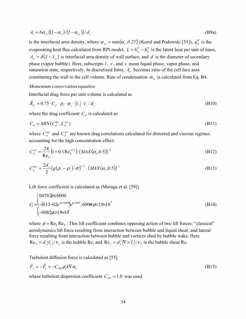
( ) ( )( ) vsvvsvi d116A // ααα −−= (B9a)

is the interfacial area density, where ( 250vsv .,min )αα = (Kurul and Podowski [55]), is the evaporating heat flux calculated from RPI model, is the latent heat per unit of mass,

Eq ′′00lsvs hhL −=

( ww xxA rr −= )δ is interfacial area density of wall surface, and is the diameter of secondary phase (vapor bubble). Here, subscripts , , and mean liquid phase, vapor phase, and saturation state, respectively. In discretized form, becomes ratio of the cell face area constituting the wall to the cell volume. Rate of condensation is calculated from Eq. B4.

dl v s

wA

vlm&

Momentum conservation equation

Interfacial drag force per unit volume is calculated as

vrrvldlv dvvCR /75.0 rrr⋅⋅⋅⋅⋅= αρ (B10)

where the drag coefficient is calculated as dC

),( visd

disdd CCMINC = (B11)

where and are known drag correlations calculated for distorted and viscous regimes accounting for the high concentration effect:

disdC vis

dC

( ) ( )( 275.0 5.0,Re1.01Re24 −⋅+= lb

b

visd MAXC α ) (B12)

( )( ) (( ) 12/1 5.0,/3

2 −⋅−= lllvdis

d MAXgd

C ασρρ ) (B13)

Lift force coefficient is calculated as (Moraga et al. [59])

⎧

×≥−

≤

5109.1 ,002.0

6000 ,0767.0

φ

φ

(B14)

where

( )⎪⎪⎨ ×<<−−= ×− 5103/36000/ 109.16000 ,2.012.0

7

φφφ eeCl

⎪⎪⎩

∇= ReRebφ . This lift coefficient comaerodynamics lift force resulting from interaction between bubble and liquid shear, and lateral

bines opposing action of two lift forces: “classical”

force resulting from interaction between bubble and vortices shed by bubble wake. Here lrvb vd ν/Re = is the bubble Re, and r

llvv vd ν/Re 2 r×∇= is the bubble shear Re.

Turbulent diffusion force is calculated as [55]

αρ ∇−=−=rr

(B15)

was used.

vlTDlv kCFF

where turbulent dispersion coefficient .1=C 0TD

54

Energy conservation equation It is reasonable to assume that the temperature of vapor inside bubbles is close to saturation. Therefore, the vapor energy conservation equation is not solved, and the temperature of vapor mass is set to saturation. The source term due to wall heating is entirely going into liquid phase:

(B16)

According to the RPI model, the total heat flux from wall to liquid is partitioned into three components:

(B17)

which are liquid convective heat flux, quenching heat flux, and evaporative heat flux. Under subcooled boiling conditions, the wall surface is subdivided into portion covered by nucleating bubbles and portion covered by fluid. Therefore, convective heat flux is expressed as

(B18)

where single phase heat transfer coefficient is derived from either log law if flow is logar c or Fourier law if flow is laminar. Liquid phase properties must be used while calcu for either turbulent or laminar flow.

Quenching heat flux models additional energy transfer related to liquid filling the wall vicinity after the bubble detachment:

(B19)

Evaporative heat flux is given by

wwl qAS ′′⋅=

EQlw qqqq ′′+′′+′′=′′

Ω ( )10 ≤Ω≤Ω−1

( )Ω−⋅−⋅=′′ 1TThq celllwlwl )(

lwhithmilating lwh

Qq ′′

( ) ( )celllwplllQ TTCfq −Ω=′′ − 5.05.02 ρκπ

Lfndq vvwE ρπ 3

6=′′ (B20)

In Eqs. B18-B20, closure must be provided for wall boiling parameters. Correct prediction of bubble departure diameter is very important because evaporation heat rate depends strongly on this parameter according to Eq. B20. It can be calculated from the following relation (Unal [60], Wei and Morel [61]):

(B21)

where all variables are in SI units. In Eq. B21:

vwd

( ) 5.0709.051042.2 −− ⋅⋅⋅⋅= θbapdvw

( )π

κρρ

spss

v

sw CTTa

2−

= (B22)

( ) ( ) ( )⎟⎟⎠⎞

⎜⎜⎝

⎛ ′′−

−=

lpll

wls

lv UCρ.q

TTMAXb00650

,/12

1ρρ

(B23)

( )0.1 ,61.0/lUMAX=θ (B24)

55

where subscript s denotes solid material of wall where boiling occurs. In Eqs. B23 and B24, an

means that b

ding h

r water boiling at atmospheric pressure.

Nucleation site de

25)

liquid temperature and velocity are local values at cells next to wall. Because FLUENT 6.2 isunstructured solver, calculation of these parameters is impossible in the general case. Again, these correlations were originally developed for use in structured or one-dimensional codes. So, instead of using local cross-section averaged values, we use local values at cell next to wall. This

ubble departure diameter will be somewhat overestimated, but bubble departure diameter is not very sensitive to local subcooling as follows from Eqs. B21 and B23. Accorto experimental data of Prodanovic et al. [62], Eqs. B21-B24 give reasonable agreement witexperiment fo

nsity is given by the following relation (Podowski [56]):

( )( ) 80.1200 satw TTn −= (B

Bubble departure frequency is calculated as

⎟⎟⎠

⎞⎜⎜⎝

⎛ ∆g ρ4=lvwd

fρ3

(B27)

(B26)

Effective wall area occupied by boiling sites is given by

( )0.1,25.0min 2 ηπ ndvw⋅=Ω

where ( )80/exp8.4 −⋅= Jaη and Jacob number is given by (Kenning and Victor [63]) ( ) ( ) 1−⋅−⋅= LTTCJa vlslpl ρρ .

Bubble diameter in free stream is givfunction of local subcooling

⎪⎨

⎧

−⋅

>⋅

= − 1105.1

5.13,105.13

sub

v

KT

d

n: one in turbulent kinetic energy and another in dissipation rate equation:

en by either constant value or by Unal correlation as a (Kurul and Podowski [55]): lsatsub TTT −=

−4

<<⋅− 5.130,0 4subsub KTT (SI units), (B28)

⎪⎩ <⋅ − 0,105.1 3

subT

Turbulence equations

Conventional mixture k-epsilon model contains two additional terms describing additional bubble stirring and dissipatio

vrvldk dvCS /75.0 2r⋅⋅⋅⋅= αρ (B29)

kv

rd Sd

vCCS

r33εε =

(Troshko and Hassan [64]).

(B30)

where 45.03 =εC

56

References 1. Webb, B.W. and Ma, C.-F., 1995, "Single-phase liquid jet impingement heat transfer",

Advances in Heat Transfer, 26, pp. 105-217. 2. Lienhard, J.H., 1995, "Liquid jet impingement", in Annual Review of Heat Transfer, pp.

199-270. 3. Garimella, S.V., 2000, "Heat Transfer and flow fields in confined jet impingement", in

Annual Review of Heat Transfer, pp. 413-494. 4. Narumanchi, S.V.J., Amon, C.H., and Murthy, J.Y., 2003, "Influence of pulsating

submerged liquid jets on chip-level thermal phenomena", ASME Journal of Electronic Packaging, 125,

5. Womac, D.J., Rrces with single circular liquid jets", ASME Journal

of Heat Transfer, 115, pp. 106-115. 6. Womac, D

impingemJournal of Heat Transfer, 116, pp. 482-486.

cteristics of arrays of free-surface liquid jets", General ASME, HTD - Vol.

n a . 1982, Tech. Report - Kansai U

9. Martin, H., 1977, "Heat and mass transfer between impinging gas jets and solid surfaces",

wa ., 1dimensional j Journal of Heat

Transfer, 112, pp. 891-898. 11. Garimella, S.V. and Rice, R.A., 1995, "Confined and submerged liquid jet impingement

heat transfer", ASME Journal of Heat12. Garimella, S.V. and Nenaydykh, B., 1996, "Nozzle-geometry effects in liquid jet

impingement heat transfer", International Journal of Heat and Mass Transfer, 39(14), pp.

ons

, D.H., Incropera, F.P., and Viskanta, R., 1993, "Jet impingement boiling", Advances in Heat Transfer, 23, pp. 1

15. Slayzak, S.J., Viskanta, R., and Incropera, F.P., 1994, "Effects of interaction between adjacent free surface planar jets on local heInternational J

16. Slayzak, S.J., Viskanta, R., and Incropera, F.P., 1994, "Effects of interactions between joining ro s on local heat transfer from the impingement

surface", ASME Journal of Heat Transfer, 116, pp. 88-95. 17. Patankar, S.V., 1980, "Numerical heat transfer and fluid flow", Taylor & Francis. 18. Fluent. User's Guide.

pp. 354-361. amadhyani, S., and Incropera, F.P., 1993, "Correlating equations for

impingement cooling of small heat sou

.J., Incropera, F.P., and Ramadhyani, S., 1994, "Correlating equations for ent cooling of small heat sources with multiple circular liquid jets", ASME

7. Pan, Y. and Webb, B.W., 1994, "Heat transfer charaPapers in Heat and Mass Transfer, Insulation and Turbomachinery, 271, pp. 23-28.

8. Yonehara, N. and Ito, I., Cooling characteristics of impinging multiple water jets ohorizontal plane niversity. p. 267-281.

Advances in Heat Transfer, 13, pp. 1-60. 10. Wadsworth, D.C. and Muda r, I 990, "Cooling of a multichip electronic module by

means of confined two- ets of dielectric liquid", ASME

Transfer, 117, pp. 871-877.

2915-2923. 13. Li, C.-Y. and Garimella, S.V., 2001, "Prandtl-number effects and generalized correlati

for confined and submerged jet impingement", International Journal of Heat and Mass Transfer, 44, pp. 3471-3480.

14. Wolf-132.

at transfer from the impingement surface", ournal of Heat and Mass Transfer, 37(2), pp. 269-282.

ad ws of circular, free-surface jet

57

19. Wadsworth, Dcritical heat flu

.C. and Mudawar, I., 1992, "Enhancement of single-phase heat transfer and x from an ultra-high-flux simulated microelectronic heat source to a

iley &

23.

24.

25. t with

ity,

6.2,

n

rectangular impinging jet of dielectric liquid", ASME Journal of Heat Transfer, 114, pp. 764-768. Zumbrunnen, D.A. and Aziz, M., 1993, "Conv20. ective heat transfer enhancement due to intermittency in an impinging jet", ASME Journal of Heat Transfer, 115, pp. 91-98. Camci, C.21. and Herr, F., 2002, "Forced convection heat transfer enhancement using a self-oscillating impinging planar jet", ASME Journal of Heat Transfer, 124, pp. 770-782. Fox, R.W. and McDonald, A.T., 1999, "Introduc22. tion to Fluid Mechanics", John WSons, Inc. Lee, D.-Y. and Vafai, K., 1999, "Comparative analysis of jet impingement and microchannel cooling for high heat flux applications", International Journal of Heat and Mass Transfer, 42, pp. 1555-1568. Rao, B.C.S. and Janakiram, K.S., 1978, "Studies on the characteristics of erosion with plainjets and jets with cavitation inducers", Journal of Testing and Evaluation, 6(6), pp. 332-340. Janakiram, K.S. and Rao, B.C.S., 1981, "Erosion studies due to liquid jet impingemenplain and cavitating jets", Journal of the Indian Institute of Science, 63(A), pp. 183-211.

26. Rao, P.V. and Buckley, D.H., 1987, "Unified empirical relations for cavitation and liquidimpingement erosion processes", Wear, 120, pp. 253-288. Thomas, G.P. and Brunton, J.H., 19727. 0, "Drop impingement erosion of metals", Proc. Roy. Soc. Lond. A, 314, pp. 549-565. Zhou, D.W. and Ma, C.F., 2004, "Local jet impingement boiling heat tr28. ansfer with R113", Heat and Mass Transfer, 40, pp. 539-549. Mudawar, I., 2000, "Assessment of high-h29. eat-flux thermal management schemes", in International conference on thermal, mechanics and thermomechanical phenomena in electronic systems, Las Vegas, NV, ASME, pp. 1-20. Mitsutake, Y. and Monde, M30. ., 2003, "Ultra high critical heat flux during forced flow boiling heat transfer with an impinging jet", ASME Journal of Heat Transfer, 125, pp. 1038-1045.

31. Liu, Z.-H., Tong, T.-F., and Qiu, Y.-H., 2004, "Critical heat flux of steady boiling for subcooled water jet impingement on the flat stagnation zone", ASME Journal of Heat Transfer, 126, pp. 179-183.

32. Copeland, R.J., 1970, "Boiling heat transfer to a water jet impinging on a flat surface (-1g)",Ph.D. thesis, Department of Mechanical Engineering, Southern Methodist UniversDallas, TX.

33. Katto, Y. and Kunihiro, M., 1973, "Study of the mechanism of burn-out in boiling system of high burn-out heat flux", Bull. JSME, 16(99), pp. 1357-1366.

34. Katto, Y. and Monde, M., 1974, "Study of mechanism of burn-out in a high heat-flux boiling system with an impinging jet", in 5th International Heat Transfer Conference, Bpp. 245-249.

35. Monde, M. and Katto, Y., 1978, "Burnout in a high heat-flux boiling system with an impinging jet", Int. J. Heat Mass Transfer, 21, pp. 295-305. Monde, M., 1980, "Burnout heat flux in saturated forced co36. nvection boiling with aimpinging jet", Heat Transfer - Japanese Research, 9(1), pp. 31-41.

58

37. Ma, C.-F. and Bergles, A.E., 1983, "Boiling jet impingement cooling of simulated microelectronic chips", in Heat Transfer in Electronic Equipment, ASME, New YorHTD-Vol. 28, pp. 5-12. Ma, C.-F.

k,

38. and Bergles, A.E., 1986, "Jet impingement nucleate boiling", Int. J. Heat Mass

39. ng

40.

, 1, FB-28, pp. 435-440. nucleate

, 65-1479.

44. t flow boiling of a mixture of

21-128.

ging jets", Heat Transfer - Japanese Research,

46. f Heat Transfer, 117, pp. 241-243.

",

48. .M., 1952, "A method of correlating heat-transfer data for surface boiling of

49. on", fer, 107, pp. 398-401.

jet

51. 985, "Critical heat flux in saturated forced convective boiling on a heated disk

52. n boiling on a heated

53. sk with multiple impinging jets", ASME Journal of Heat Transfer, 113, pp.

54. se electronic cooling using

Transfer, 29(8), pp. 1095-1101. Ruch, M.A. and Holman, J.P., 1975, "Boiling heat transfer to a Freon-113 jet impingiupward onto a flat, heated surface", Int. J. Heat Mass Transfer, 18, pp. 51-60. Katto, Y. and Ishii, K., 1978, "Burnout in a high heat flux boiling system with a forcedsupply of liquid through a plane jet", in Proceedings of the 6th International Heat TransferConference

41. Miyasaka, Y., Inada, S., and Owase, Y., 1980, "Critical heat flux and subcooledboiling in transient region between a two-dimensional water jet and a heated surface", J. Chem. Eng. Jpn., 13, pp. 29-35.

42. Mudawar, I. and Wadsworth, D.C., 1991, "Critical heat flux from a simulated chip to a confined rectangular impinging jet of dielectric liquid", Int. J. Heat Mass Transfer, 34(6)pp. 14

43. Nonn, T., Dagan, Z., and Jiji, L.M., 1988, "Boiling jet impingement cooling of simulated microelectronic heat sources", in Winter Annual Meeting, Chicago, Illinois, ASME, 88-WA/EEP-3, pp. 1-9. Nonn, T., Dagan, Z., and Jiji, L.M., 1989, "Jet impingemenFC-72 and FC-87 liquids on a simulated electronic chip", in National Heat Transfer Conference, HTD-Vol. 111, pp. 1

45. Monde, M., Kusuda, H., and Uehara, H., 1982, "Burnout heat flux in saturated forced convection boiling with two or more impinpp. 18-31. Monde, M. and Mitsutake, Y., 1996, "Critical heat flux in forced convective subcooledboiling with multiple impinging jets", ASME Journal o

47. Pais, M.R., Chow, L.C., and Mahefkey, E.T., 1993, "Multiple jet impingement coolingJournal of Thermophysics and Heat Transfer, 7(3), pp. 435-440. Rohsenow, Wliquids", Trans. Am. Soc. Mech. Engrs., Paper No. 51-A110, 74, pp. 969-976. Sharan, A. and Lienhard, J.H., 1985, "On predicting burnout in the jet-disk configuratiASME Journal of Heat Trans

50. Katto, Y. and Yokoya, S., 1988, "Critical heat flux on a disk heater cooled by a circularof saturated liquid impinging at the center", Int. J. Heat Mass Transfer, 31(2), pp. 219-227. Monde, M., 1with an impinging jet", Warme-und Stoffubertragung, 19, pp. 205-209. Monde, M., 1987, "Critical heat flux in saturated forced convectiodisk with an impinging jet", ASME Journal of Heat Transfer, 109, pp. 991-996. Monde, M. and Inoue, T., 1991, "Critical heat flux in saturated forced convective boiling on a heated di722-727. Estes, K.A. and Mudawar, I., 1995, "Comparison of two-phafree jets and sprays", ASME Journal of Electronic Packaging, 117, pp. 323-332.

59

55. Kurul, N. and Podowski, M.Z., 1990, "Multidimensional effects in forced convectiosubcooled boiling", in Ninth International Heat Transfer Conference, Jerusalem, Israel,BO-04, pp. 21-26.

n 1-

Eighth International Topical Meeting on Nuclear Reactor

57. se jet

58. d computation of heat exchanges in the configuration

59. ahey, R.T., 1999, "Lateral forces on spheres in turbulent

60. g the subcooled nucleate flow boiling of water up to 17.7 MN/m ", Int. J.

61. o-luid model", in Proceedings of ICONE 10, Arlington, VA, USA, 10,

62. phase Flow, 28(1), pp. 1-19.

),

32.

56. Podowski, R.M., et al., 1997, "A mechanistic model of the ebullition cycle in forced convection subcooled boiling", inThermal-Hydraulics, Kyoto, Japan, 3, pp. 1535-1542. Wang, D., Yu, E., and Przekwas, A., 1999, "A computational study of two phaimpingement cooling of an electronic chip", in Fifteenth IEEE Semi-therm Symposium,IEEE, pp. 10-15. Seiler, N., et al., 2003, "Modeling anof an impinging jet on a hot plate", in International conference on supercomputing in nuclear applications, SNA 2003, Paris, France, pp. 1-13. Moraga, F.J., Bonetto, F.J., and Luniform shear flow", International Journal of Multiphase Flow, 25, pp. 1321-1372. Unal, H.C., 1976, "Maximum bubble diameter, maximum bubble-growth time and bubble-growth rate durin 2

Heat Mass Transfer, 19, pp. 643-649. Wei, Y. and Morel, C., 2002, "Prediction of parameters distribution of upward boiling twphase flow with two-fpp. Prodanovic, V.A., 2002, "Bubble behavior in subcooled flow boiling of water at low pressures and low flow rates", Int. J. Multi

63. Kenning, D.B.R. and Victor, H.T., 1981, "Fully-developed nucleate boiling: overlap ofareas of influence and interference between bubble sites", Int. J. Heat Mass Transfer, 24(6pp. 1025-10

64. Troshko, A.A. and Hassan, Y.A., 2001, "A two-equation turbulence model of turbulent bubbly flows", International Journal of Multiphase Flow, 27, pp. 1965-2000.

60

F1147-E(12/2004)

REPORT DOCUMENTATION PAGE Form Approved OMB No. 0704-0188

The public reporting burden for this collection of information is estimated to average 1 hour per response, including the time for reviewing instructions, searching existing data sources, gathering and maintaining the data needed, and completing and reviewing the collection of information. Send comments regarding this burden estimate or any other aspect of this collection of information, including suggestions for reducing the burden, to Department of Defense, Executive Services and Communications Directorate (0704-0188). Respondents should be aware that notwithstanding any other provision of law, no person shall be subject to any penalty for failing to comply with a collection of information if it does not display a currently valid OMB control number. PLEASE DO NOT RETURN YOUR FORM TO THE ABOVE ORGANIZATION. 1. REPORT DATE (DD-MM-YYYY)

December 2005 2. REPORT TYPE

Technical Report 3. DATES COVERED (From - To)

5a. CONTRACT NUMBER

DE-AC36-99-GO10337

5b. GRANT NUMBER

4. TITLE AND SUBTITLE Modeling Single-Phase and Boiling Liquid Jet Impingement Cooling in Power Electronics

5c. PROGRAM ELEMENT NUMBER

5d. PROJECT NUMBER NREL/TP-540-38787

5e. TASK NUMBER FC067010

6. AUTHOR(S) S.V.J. Narumanchi, V. Hassani, and D. Bharathan

5f. WORK UNIT NUMBER

7. PERFORMING ORGANIZATION NAME(S) AND ADDRESS(ES) National Renewable Energy Laboratory 1617 Cole Blvd. Golden, CO 80401-3393

8. PERFORMING ORGANIZATION REPORT NUMBER NREL/TP-540-38787

10. SPONSOR/MONITOR'S ACRONYM(S) NREL

9. SPONSORING/MONITORING AGENCY NAME(S) AND ADDRESS(ES)

11. SPONSORING/MONITORING AGENCY REPORT NUMBER

12. DISTRIBUTION AVAILABILITY STATEMENT National Technical Information Service U.S. Department of Commerce 5285 Port Royal Road Springfield, VA 22161

13. SUPPLEMENTARY NOTES

14. ABSTRACT (Maximum 200 Words) Jet impingement has been an attractive cooling option in a number of industries over the past few decades. Over the past 15 years, jet impingement has been explored as a cooling option in microelectronics. Recently, interest has been expressed by the automotive industry in exploring jet impingement for cooling power electronics components. This technical report explores, from a modeling perspective, both single-phase and boiling jet impingement cooling in power electronics, primarily from a heat transfer viewpoint. The discussion is from the viewpoint of the cooling of IGBTs (insulated-gate bipolar transistors), which are found in hybrid automobile inverters.

15. SUBJECT TERMS Power electronics cooling; jet impingement cooling; modeling liquid jet impingement; automotive power electronics cooling; hybrid automotive inverters; cooling IGBTs

16. SECURITY CLASSIFICATION OF: 19a. NAME OF RESPONSIBLE PERSON a. REPORT

Unclassified b. ABSTRACT Unclassified

c. THIS PAGE Unclassified

17. LIMITATION OF ABSTRACT

UL

18. NUMBER OF PAGES

19b. TELEPHONE NUMBER (Include area code)

Standard Form 298 (Rev. 8/98) Prescribed by ANSI Std. Z39.18

modeling single-phase and boiling liquid jet impingement cooling

Documents