impact of evaluation methods on decision tree accuracy
TRANSCRIPT

Impact of Evaluation Methods on Decision Tree Accuracy
Batuhan Baykara
University of Tampere
School of Information Sciences
Computer Science
M.Sc. thesis
Supervisor: Prof. Martti Juhola
April 2015
i
University of Tampere
School of Information Sciences
Computer Science
Batuhan Baykara: Impact of Evaluation Methods on Decision Tree Accuracy
M.Sc. thesis, 72 pages, 6 index pages
April 2015
Decision trees are one of the most powerful and commonly used supervised learning
algorithms in the field of data mining. It is important that a decision tree performs
accurately when employed on unseen data; therefore, evaluation methods are used to
measure the predictive performance of a decision tree classifier. However, the
predictive accuracy of a decision tree is also dependant on the evaluation method
chosen since training and testing sets of decision tree models are selected according to
the evaluation methods.
The aim of this thesis was to study and understand how using different evaluation
methods might have an impact on decision tree accuracies when they are applied to
different decision tree algorithms. Consequently, comprehensive research was made on
decision trees and evaluation methods. Additionally, an experiment was conducted
using ten different datasets, five decision tree algorithms and five different evaluation
methods in order to study the relationship between evaluation methods and decision tree
accuracies.
The decision tree inducers were tested with Leave-one-out, 5-Fold Cross Validation,
10-Fold Cross Validation, Holdout 50 split and Holdout 66 split evaluation methods.
According to the results, cross validation methods were superior to holdout methods in
overall. Moreover, Holdout 50 split has performed the poorest in most of the datasets.
The possible reasons behind these results have also been discussed in the thesis.
Key words and terms: Data Mining, Machine Learning, Decision Tree, Accuracy,
Evaluation Methods.

ii
Acknowledgements
I wish to express my sincere gratitude to my supervisor Professor Martti Juhola who
have guided and encouraged me throughout this thesis. Additionally, I would like to
thank Kati Iltanen for her support and valuable comments.
I would also like to thank my parents and my little sister for their continued support and
motivation throughout my life.
March 2015, Tampere
Batuhan Baykara

iii
Table of Contents
1. Introduction ...................................................................................................................... 1
1.1. Research Questions ................................................................................................... 2
1.2. Structure of the Thesis ............................................................................................... 2
2. Knowledge Discovery in Databases (KDD) .......................................................................... 3
2.1. Data Mining ............................................................................................................... 5
2.2. Machine Learning ...................................................................................................... 7
2.2.1. Supervised Learning ........................................................................................... 8
2.2.2. Unsupervised Learning ....................................................................................... 9
2.2.3. Semi-Supervised Learning .................................................................................. 9
2.2.4. Reinforcement Learning ................................................................................... 10
2.3. What is the difference between KDD, Data Mining and Machine Learning? ............. 10
3. Decision Trees ................................................................................................................. 12
3.1. Univariate Decision Trees ........................................................................................ 14
3.1.1. Attribute Selection Criteria............................................................................... 17
3.1.1.1. Information Gain ...................................................................................... 18
3.1.1.2. Gain Ratio ................................................................................................ 19
3.1.1.3. Gini Index ................................................................................................. 20
3.1.1.4. Twoing Criterion ....................................................................................... 21
3.1.1.5. Chi-squared Criterion ............................................................................... 21
3.1.1.6. Continuous Attribute Split ........................................................................ 22
3.1.2. Pruning Methods ............................................................................................. 22
3.1.2.1. Cost Complexity Pruning .......................................................................... 25
3.1.2.2. Reduced Error Pruning ............................................................................. 25
3.1.2.3. Pessimistic Pruning ................................................................................... 26
3.1.2.4. Minimum Error Pruning ............................................................................ 26
3.1.2.5. Error Based Pruning.................................................................................. 27
3.1.3. Decision Tree Induction.................................................................................... 28
3.1.3.1. ID3 ........................................................................................................... 29
3.1.3.2. C4.5 .......................................................................................................... 30
3.1.3.3. C5.0 .......................................................................................................... 31
3.1.3.4. CART ........................................................................................................ 31
3.1.3.5. CHAID....................................................................................................... 32
3.1.4. Rule sets .......................................................................................................... 32
iv
3.1.5. Advantages and Disadvantages of Decision Trees ............................................. 34
3.2. Multivariate decision trees ...................................................................................... 36
4. Evaluation of Decision Trees ............................................................................................ 37
4.1. Performance Evaluation Metrics and Measures ....................................................... 37
4.2. Accuracy Estimating Methodologies ........................................................................ 40
4.2.1. Holdout Method .............................................................................................. 41
4.2.2. K-Fold Cross Validation .................................................................................... 42
4.2.3. Leave-one-out Method .................................................................................... 43
4.2.4. Bootstrapping .................................................................................................. 44
5. Research Method ............................................................................................................ 46
5.1. Motivation and Purpose of the Experiment.............................................................. 46
5.2. Datasets .................................................................................................................. 47
5.2.1. Detailed Dataset Explanations .......................................................................... 48
5.2.2. Preprocessing the Datasets .............................................................................. 51
5.3. Algorithms and Evaluation Methods Chosen ............................................................ 54
5.4. Tools Used ............................................................................................................... 55
5.4.1. WEKA ............................................................................................................... 55
5.4.2. IBM SPSS Modeler............................................................................................ 55
5.4.3. C5.0/See5 ........................................................................................................ 56
5.4.4. RapidMiner ...................................................................................................... 56
5.4.5. Other Tools ...................................................................................................... 57
6. Results ............................................................................................................................ 58
6.1. Result Evaluation ..................................................................................................... 63
7. Discussion and Conclusion ............................................................................................... 67
References .............................................................................................................................. 69
v
List of Figures
Figure 2.1. KDD process .......................................................................................................... 4
Figure 2.2. Machine learning process ...................................................................................... 8
Figure 3.1. PlayTennis example. ............................................................................................. 13
Figure 3.2. Branching types..................................................................................................... 15
Figure 3.3. Post-pruning example ............................................................................................ 23
Figure 3.4. TDIDT family ...................................................................................................... 28
Figure 3.5. Example tree. ........................................................................................................ 34
Figure 4.1. Confusion matrix examples. .................................................................................. 38
Figure 4.2. Detailed confusion matrix ..................................................................................... 39
Figure 4.3. Holdout method..................................................................................................... 41
Figure 4.4. K-Fold cross validation. ........................................................................................ 42

vi
List of Tables
Table 5.1. Dataset summary. ................................................................................................... 48
Table 5.2. Arrhythmia missing values. .................................................................................... 52
Table 5.3. Audiology missing values. ...................................................................................... 53
Table 5.4. Breast cancer missing values................................................................................... 53
Table 5.5. Hepatitis missing values. ........................................................................................ 53
Table 6.1. Arrhythmia test results. ........................................................................................... 59
Table 6.2. Audiology test results. ............................................................................................ 59
Table 6.3. Balance scale test results. ........................................................................................ 60
Table 6.4. Breast cancer test results. ........................................................................................ 60
Table 6.5. Glass test results. .................................................................................................... 61
Table 6.6. Hepatitis test results. ............................................................................................... 61
Table 6.7. Ionosphere test results. ............................................................................................ 62
Table 6.8. Iris test results. ....................................................................................................... 62
Table 6.9. Musk1 test results. .................................................................................................. 62
Table 6.10. Zoo test results...................................................................................................... 63
Table 6.11. Combined test results. ........................................................................................... 65

1
1. Introduction
For the past 20-30 years, the amount of data that has been digitalized or has been
gathered through digital environments such as the web has been in significant amounts.
It has been estimated that the amount of stored information doubles every 20 months
[Rokach and Maimon, 2014]. As a result, it has become impossible to digest the
gathered data manually by people and the need for other solutions that would enable
mankind to process the gathered data easier has arisen. Therefore, different data analysis
techniques have recently had vital importance in various areas: public health and
healthcare, science and research, law enforcement, financial business areas and
customer targeted commercial areas. Especially with the recent advancement in social
media services, immense amount of user data are being gathered and processed on daily
basis [Mosley Jr, 2012].
Receiving large amount of data has given companies, governments and private
people an opportunity to use these raw data and turn them into valuable information.
For instance, companies have started improving their businesses by the help of data.
Business intelligence (BI) and business analytics (BA) are two examples of business
enhancement techniques which are applied to existing large amount of data the
companies have gathered. Then the findings are used for future planning and decision
making in order to increase company’s profit margin. In order to make use of large
amount of data, some processes and techniques need to be applied. Data mining (DM),
machine learning (ML) and knowledge discovery in databases (KDD) are the processes
that enable turning data into useful knowledge. Application of these processes has
become more common for the past years and is becoming even more frequent.
Data mining is one of the mostly applied processes to make use of large amount of
data. There are different types of data mining objectives but the two most commonly
used are predictive modeling and descriptive modeling. Predictive modeling is essential
because through this task one can make predictions about the future by learning from
the previous data. This can be considered as a frequently applied task within the concept
of data mining. The predictive modeling objective is accomplished by making use of
various machine learning or data mining algorithms such as decision tree induction
algorithms. As it can be understood from the objective’s title, there needs to be a model
that could be used to make predictions from the learned data. Therefore, a model is built
from existing data by the help an algorithm where decision tree induction algorithms
can be considered as a good example. Later on, this model is used to make predictions
on the new unseen data.
Decision tree performances are evaluated according to the level of accuracy
obtained from the predictions that are made. Hence, accuracy is one of the most
important evaluation measures for decision trees. In order to make good and stable
predictions from the model, accuracy obtained from the decision tree model needs to be
high. However, there are various reasons that might affect the accuracy of decision tree
2
models negatively as well as positively. One of the possible reasons that might affect
accuracy is the evaluation method that is chosen for the decision tree induction. The
portions of the data to be used when the model is being built are decided according to
the choice of the evaluation method. Thus, the resulting accuracy of a decision tree is
dependent on the evaluation method that is chosen in the beginning of the induction
process.
Even though decision trees are widely and frequently applied in data mining and
machine learning context, there are not many studies that have made comparisons of
different decision tree algorithms when evaluated by different methods in terms of
performance. Therefore, the aim of this thesis is to study and understand how using
different evaluation methods might have an impact on decision tree accuracies when
they are applied to different decision tree algorithms.
1.1. Research Questions
As stated earlier in the introduction, the resulting accuracy of a decision tree on unseen
cases is dependent on the evaluation method. However, the degree of dependency and
the best overall evaluation method is unknown. Therefore, the main aim of this thesis is
to study the effects of evaluation methods on decision tree predictive performance
measures. Accordingly, the research questions that are going to be answered in this
thesis are given below;
1) How much does the evaluation method chosen affect the predictive
performance of decision trees?
2) Which evaluation method is superior to others in most cases?
1.2. Structure of the Thesis
The thesis is structured in the following way. After the introduction, background
information about the research field is given. Data mining, machine learning and
knowledge discovery are explained in detail and the differences between them are also
discussed. After the second part of the thesis, decision tree topic is explained in a
comprehensive manner so that the all literature knowledge needed in the experimental
part of the thesis is covered thoroughly. Decision tree structure is explained first and
then univariate decision trees are discussed in detail. Univariate topic includes the
subtopics of: attribute selection criteria, pruning methods, decision tree induction,
rulesets and advantages and disadvantages of decision trees. Afterwards, various state of
the art evaluation methods are explained. When all the literature regarding the thesis is
given, research methodology is explained. All the necessary background information
about the experimental part of the thesis are discussed in the research methodology part.
Lastly, the results are explained which finally lead to a brief discussion and conclusion
part.

3
2. Knowledge Discovery in Databases (KDD)
The terms data mining and knowledge discovery in databases have been very popular
for fields of research, industry and media attention especially since the 1990's. There is
not a conventional or universally used term that can summarize the objective of
obtaining valuable knowledge from some data. However, the mostly agreed term that
generalizes the process is; knowledge discovery in databases. “There is an urgent need
for a new generation of computational theories and tools to assist humans in extracting
useful information (knowledge) from the rapidly growing volumes of digital data. These
theories and tools are the subject of the emerging field of knowledge discovery in
databases (KDD) [Fayyad et al., 1996].”
KDD is vital because its application areas are very wide. Besides research, the main
business KDD application areas include marketing, finance, fraud detection,
manufacturing, telecommunications, and internet agents [Fayyad et al., 1996]. Of
course the area keeps expanding as days go by and now with the emerge of social
media, the application areas have started to shift towards processing raw data that are
being gathered from social sites to give leverage to a company or an organization. This
is mainly because the digital data that has been gathered through social sites and the
internet increased in large amounts. A recent and interesting example is the prediction
of flu trends [Han and Kamber, 2006]. Google, which is a world leading technology
firm and a search engine in the core, is receiving hundreds of millions of queries every
day. After processing those queries, Google has actually found out that a relation
between the number of people who have searched for flu related information exists with
the number of people who actually have flu symptoms. By the help of such analytics,
flu trends and activities can be estimated 2 weeks earlier than the traditional systems
can. This is just one example why KDD can be very important when it comes to
turning great amount of data to knowledge that might have great importance.
KDD cannot be seen as a single process; it is a process which has sub processes
within each other. Thus, it combines various different research fields according to the
objective of KDD process and the data that is going to be used. Some fields that are
considered part of KDD are; machine learning, data mining, pattern recognition,
databases, database management systems, statistics, artificial intelligence (AI),
knowledge acquisition for expert systems, data visualization and high performance
computing [Fayyad et al., 1996]. All these are combined to make one large process of
KDD which is generalized in 9 steps. A scheme for KDD is below in Figure 2.1.
4
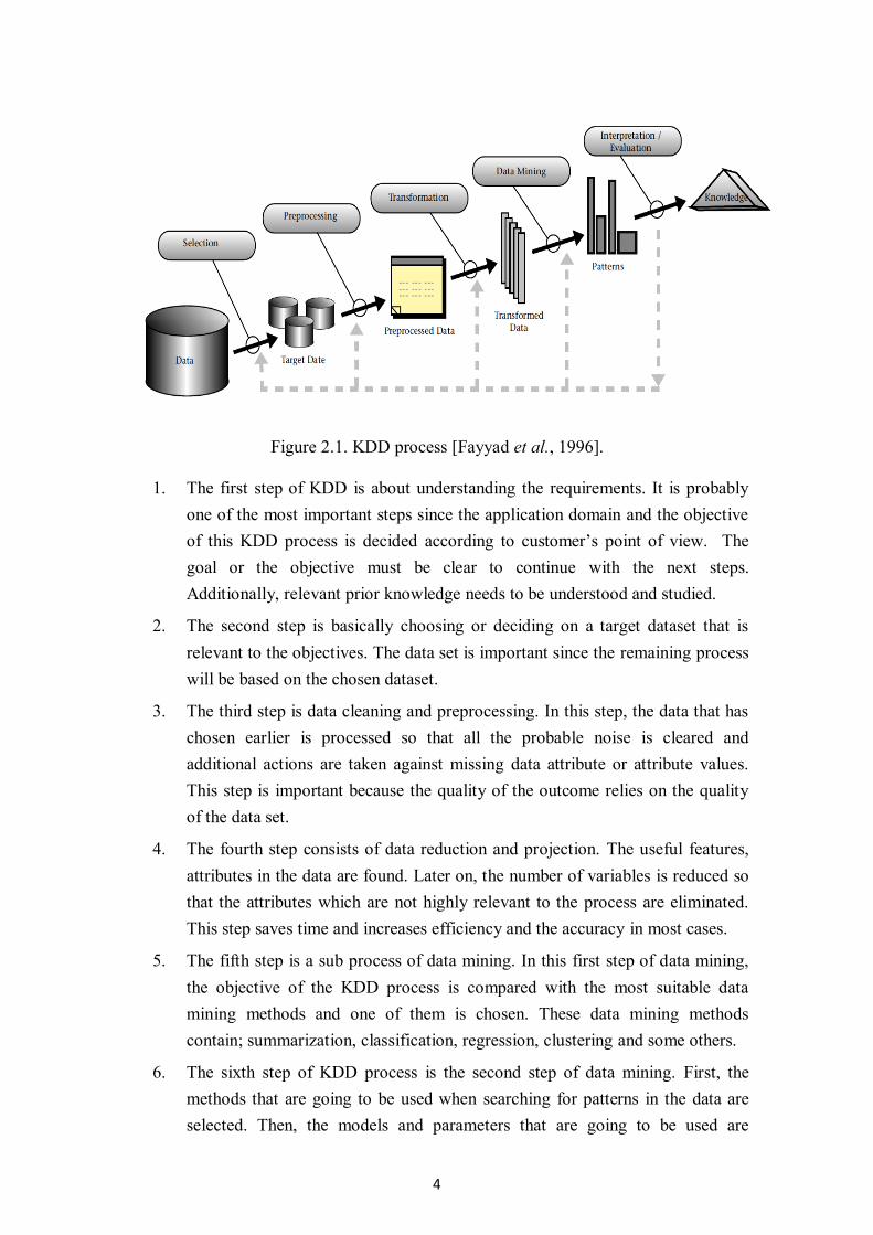
Figure 2.1. KDD process [Fayyad et al., 1996].
1. The first step of KDD is about understanding the requirements. It is probably
one of the most important steps since the application domain and the objective
of this KDD process is decided according to customer’s point of view. The
goal or the objective must be clear to continue with the next steps.
Additionally, relevant prior knowledge needs to be understood and studied.
2. The second step is basically choosing or deciding on a target dataset that is
relevant to the objectives. The data set is important since the remaining process
will be based on the chosen dataset.
3. The third step is data cleaning and preprocessing. In this step, the data that has
chosen earlier is processed so that all the probable noise is cleared and
additional actions are taken against missing data attribute or attribute values.
This step is important because the quality of the outcome relies on the quality
of the data set.
4. The fourth step consists of data reduction and projection. The useful features,
attributes in the data are found. Later on, the number of variables is reduced so
that the attributes which are not highly relevant to the process are eliminated.
This step saves time and increases efficiency and the accuracy in most cases.
5. The fifth step is a sub process of data mining. In this first step of data mining,
the objective of the KDD process is compared with the most suitable data
mining methods and one of them is chosen. These data mining methods
contain; summarization, classification, regression, clustering and some others.
6. The sixth step of KDD process is the second step of data mining. First, the
methods that are going to be used when searching for patterns in the data are
selected. Then, the models and parameters that are going to be used are
5
selected according to the data mining method chosen and the overall KDD
process objectives.
7. The seventh step is the last step of data mining process. In this step, the
methods and models that are chosen are applied to the dataset. Patterns that
might be interesting are searched for by being represented as classification
rules or trees, regression and clustering.
8. The eight step is the evaluation of the data mining results. The patterns that are
found or the data that has been summarized are examined in order to find
something useful. If not, the earlier steps can be repeated until something that
is relevant or useful is found.
9. The ninth, last step is consolidation of the found knowledge. The knowledge
that has been found is presented to the user in a clear and easily understandable
fashion.
This is the generalization of the KDD process and its steps. Some of these steps can
be skipped or combined according to the needs of users. As mentioned earlier, the steps
can be seen as iteration points or loops; therefore, some steps can be repeated to gain
better results.
2.1. Data Mining
“Data mining is the analysis of (often large) observational data sets to find unsuspected
relationships and to summarize the data in novel ways that are both understandable and
useful to the data owner [Hand et al., 2001].” To put it shortly, it is the process of
discovering interesting patterns and knowledge from large amount of data. Data mining
is formed in the intersection of various different fields such as: artificial intelligence,
machine learning, statistics and database systems. Machine learning is an important
field for data mining because most of the algorithms that are used in data mining
methods belong to algorithms that exist in machine learning field. In the beginning, data
mining term was mostly used by statisticians, database researchers and business
communities; however, nowadays it seems such a term is used by everyone to refer to
the whole KDD process [Jackson, 2002].
Data mining has its own purposes or tasks;
Exploratory Data Analysis: The task is to find a useful or rational connection
between variables through exploring the data. However, the main issue is there
are not any prior objectives or ideas when going through the exploration. It is
in random fashion and is based on interactive and visual techniques. The data
scientist try to spot an interesting pattern of information by visually analyzing
the obtained charts. Such a method can be very effective at times, mostly with
small datasets that have less number of variables; the human perspective can
analyze and spot some interesting patterns that machine and algorithms might
6
not. Some plots that are used to support the visual analysis process can be
scatter plots, box plots, pie charts and so on. Additionally, as dimensionality
increases it becomes harder to visualize the data thus leading to inefficient data
exploration results [Hand et al., 2001].
Descriptive Modeling: As it can be understood from the title, the task is to
describe the data. Some descriptive methods or models are; overall probability
distribution (density estimation), cluster analysis and dependency modeling
[Hand et al., 2001]. For example in cluster analysis the data is divided into
groups so that the data instances that are more related and close to each other
fall into the same groups. It is considered to be one of the most powerful
methodologies in descriptive modeling and in data mining.
Predictive Modeling: The main task is to make predictions and estimates on
new instances based on the models that have been built by examining the
already existing data instances [Hand et al., 2001]. It has two subcategories;
classification and regression. The difference between them is the target
attribute of classification models are categorical where as regression models are
numerical or quantitative. There have been many developments and
breakthroughs in predictive modeling thank to fields of machine learning and
statistics. One of those developments is decision trees and it is in the group of
predictive modeling. Decision trees are one of the most powerful and widely
used methods in the field.
Discovering patterns and rules: This task is different from the previously
mentioned ones since it does not require model building [Hand et al., 2001].
The main objective is to find interesting patterns in the existing data using
pattern detection or recognition methods. The most important example is
market database transactions. The aim is to find items that are bought
frequently and in accordingly with other items so that a frequent item set is
found. Then these frequent itemsets are used to assess and find relevant
patterns in the data. Such kind of pattern finding is called association rule
mining.
Retrieval by content: This task is also related with pattern finding and matching
instead of model building. The aim is to find patterns in the data that are
defined earlier or desired. Retrieval by content is used for image or text based
datasets mostly [Hand et al., 2001]. Similarity is the key measure in this task.
For example, image data are processed so that a sample image, sketch or
description is given beforehand to retrieve relevant image from the data. In text
based datasets, keywords can be the key similarity measure and such keyword
can be searched for in text based documents such as Word files, PDF files or
even Web pages.
7
The process of data mining has tried to be standardized throughout the years, which
eventually lead to two mostly used standards; CRISP-DM and SEMMA [Jackson,
2002]. Cross Industry Standard Process for Data Mining (CRISP-DM) is one of the
leading process methodologies for data mining that is used. The basic steps and
principle are almost identical to KDD process. It consists of the following steps:
business understanding, data understanding, data preparation, modeling, evaluation and
deployment. SEMMA is another process which actually is an acronym for its steps;
sample, explore, modify, model and assess. CRISP-DM is more widely used than
SEMMA.
2.2. Machine Learning
Machine learning (ML) is a field that was born from the field of artificial intelligence
(AI). Although being a computer science field, it is closely related with statistics and
many other fields such as philosophy, information theory, biology, cognitive science,
computational complexity and control theory. The main question that lead to the birth of
machine learning was: Can a machine be thought to think like human beings and learn?
This question was mainly raised after Alan Touring’s paper: “Computing Machinery
and Intelligence” and his research question: “Can machines think?” [Turing, 1950].
There were concentrated researches on ML and some important discoveries were made
such as perceptrons and neural networks. However, later on machine learning was left
outside the field of AI due to ML’s emphasis on logical and knowledge based approach.
Hence, both fields were separated and afterwards machine learning flourished in the
1990s as a separate field and started improving and expanding rapidly.
A clear definition that was given by Tom Mitchell declares machine learning as: "A
computer program is said to learn from experience E with respect to some class of tasks
T and performance measure P, if its performance at tasks in T, as measured by P,
improves with experience E [Mitchell, 1997].” Therefore, machine learning is the
science of teaching the machines to learn by itself with the use of existing data and
algorithms. The learning process is usually done through a model that is learned from
the existing data and this model is used for future predictions and acts. The model is
updated constantly or to put it in different words, the model learns at it sees new data.
The figure 2.2 below illustrates the machine learning process in a very clear and
detailed way.

8
Figure 2.2. Machine learning process [Lai et al., 2007].
In the first step of the process, data that is going to be used for the machine learning
purpose is gathered and transformed into a proper form. Then this data is divided into
three parts; training, testing and validation data. However, the data is usually divided
into two parts training and testing. Validation data is mostly used in neural networks
since its hidden nodes require another step of validating the hidden nodes. Afterwards
the training data is used in training phase of the process to learn the data and build a
model. Then, the acquired models are tested with the separate testing data to correct or
evaluate the models. The best model is chosen amongst the models at the testing phase.
If it is a specific algorithm that requires one more level of validation like neural
networks, the evaluation of models is made at validation level. If none of the models are
at satisfactory level, then the process is repeated until a specified quality is reached or
the process is quit. After the model is chosen, it means the model chosen is ready for
practical applications and is able to make predictions, learn and evolve with the system.
There are lots of machine learning algorithms and all of them have different type of
methodologies or structures; however, the algorithms can be differentiated from each
other in some level and be grouped according to some characteristics of their own.
Consequently, there are four different kinds of learning groups in which the algorithms
are grouped in; supervised learning, unsupervised learning, semi-supervised learning
and reinforcement learning.
2.2.1. Supervised Learning
In supervised learning, the data must have labeled attributes for inputs and most
importantly an attribute labeled for the desired output value [Alpaydin, 2014]. Each
data instance should have one variable that designates the desired output value
according to its input values or variables. The input variables should be important
factors in determining the output value, and should be kept at a reasonable and effective
9
amount. The output value can either be a categorical (for classification tasks) or
continuous (for regression tasks). These two types of tasks are used in decision tree
learning, which is a supervised algorithm, and will be explained in detail in the further
chapters.
The goal of supervised learning is to build a model that represents the training data
correctly and in a simple manner. The model is assessed before it is chosen amongst
other models according to its accuracy, precision or recall rate [Lai et al., 2007].
Additionally, it might be assessed and improved after it is being used in practical
solutions as well. Most commonly used algorithms in supervised learning besides
decision trees are; artificial neural networks, kernel estimators, naïve Bayes classifiers,
nearest neighbor algorithms, support vector machines and random forests (decision trees
with ensemble methods). Supervised learning algorithms’ application areas include;
bioinformatics, database marketing, information retrieval and more commonly pattern
recognition areas (image, voice and speech recognition).
2.2.2. Unsupervised Learning
Unlike supervised learning, the data does not have any prior output label. Therefore, the
algorithms’ main purpose is to learn the data by itself since the data is unlabeled.
Regularities, patterns or any kind of commonalities between the data samples are
investigated and tried to be grouped so that the data that are related to each other are in
the same group [Lai et al., 2007]. It is closely related with density estimation in
statistics [Alpaydin, 2014]. Three of the important unsupervised learning algorithms are
clustering, principal component analysis and EM algorithm. Clustering algorithm also
has its own various methodologies to group the data; k-means algorithm, mixture
models, hierarchical clustering and some other methodologies. However, the main goal
is to group the data instances in a way that the instances in the same group are called
clusters and the instances within the clusters are more similar to each other than in any
other instances that belong to different clusters. In other words, intracluster similarity is
high and intercluster similarity is low. Principal component analysis (PCA) is used for
reduction of the number of variables or dimensions in the data so that for example the
performance of learning can be maximized. Other important unsupervised method, the
expectation-maximization (EM) algorithm tries to maximize the likelihood of
parameters in the model acquired from the data in cases where equations in the learning
process cannot be solved directly.
2.2.3. Semi-Supervised Learning
As it can be understood from the title, semi-supervised learning is a group of supervised
learning algorithms and tasks that also make use of unsupervised learning or in other
words unlabelled data. The data used in semi-supervised learning mostly consists of

10
unlabelled data and a small amount of labeled data. The main reason to combine both
learning methods is to increase overall accuracy of the learning process. It has proven to
be better than the other supervised methods under some circumstances [Lai et al.,
2007]. A downside of semi-supervision exists; the labeled data needs to be generated by
highly skilled human beings thus making the whole process more expensive.
Semi-supervised learning can also be referred to as transductive learning or
inductive learning. It makes use of supervised and unsupervised learning algorithms and
combines the strengths from both sides to generate a semi-supervised algorithm. Some
semi-supervised methods are; self-training, mixture models, co-training and multiview
learning, graph based methods and semi-supervised support vector machines.
2.2.4. Reinforcement Learning
“Reinforcement learning (RL) is an approach to machine intelligence that combines the
fields of dynamic programming and supervised learning to yield powerful machine
learning systems [Lai et al., 2007].” A decision making agent, assume a robot, is given
a goal and the robot tries to reach that goal through learning by itself and acting back
and forth with an environment. Therefore, some key rules needs to be satisfied for a
basic RL model and these include;
1. A set of environment states.
2. A set of actions.
3. A set of rules for transitioning between states.
4. A set of rules for determining the rewards that are given at the end of
transitions.
5. A set of rules that describe what the agent or the robot observes.
Some of the best applications of reinforcement learning are game playing activities.
Since the games require a vast amount of state space, reinforcement methods come in
handy and learn from the human opponents while playing. Instead of the traditional
game AIs which require brute force search amongst the state space, RL can achieve
better results faster than the traditional methods.
2.3. What is the difference between KDD, Data Mining and Machine Learning?
After discussing the three topics, KDD, data mining and machine learning, all these
areas seem very similar and overlapped with each other. This would raise the question:
How are all these areas different than each other? There are different opinions on such a
question because to some people, the definitions of KDD and data mining differ.
However, according to the majority there is a connection between all these subjects, a
linkage.

11
As mentioned earlier, KDD is a process to turn digital data into knowledge and if
we were to make a connection between KDD and data mining, data mining is
considered as a sub process of KDD. KDD focuses on the whole process rather than just
the analysis part; therefore, it can be considered as a multidisciplinary activity which
encapsulates data mining as the core data analysis part to its own process. Now that the
difference between KDD and data mining is clear, what about machine learning and
how is it different than data mining? This is probably a more difficult question than the
first one since the line between both subjects is very thin. Machine learning and data
mining tries to solve the similar type of problems and the reason behind it is simple;
data mining makes use of machine learning algorithms in its own process. Data mining
itself also has some processes and the core of all data mining processes depends on the
algorithms used in it. These algorithms belong to machine learning field. Consequently,
machine learning is the study and development of algorithms that enable computers to
learn without being explicitly programmed where as data mining concentrates on a
bigger process which utilizes those algorithms and tries to find interesting patterns and
structures in the data. To sum up, machine learning is the field which aids data mining
in its process by providing algorithms. Moreover, data mining is the sub process of
KDD where the data is processed and analyzed in order to turn the raw data into
knowledge.

12
3. Decision Trees
Decision trees are in the group of supervised learning methods within the concept of
data mining and machine learning. Decision trees create solutions to classification
problems on various different fields such as engineering, science, medical fields and
other related fields. Thus, decision trees are considered to be one of the most powerful
tools that can accomplish classification and prediction tasks [Kantardzic, 2011].
Decision trees can be considered as a non-parametric method since no assumption is
made for the class densities and the tree structure or the model is not known before the
tree growing process [Alpaydin, 2014]. As mentioned earlier, decision trees are used for
predictive analysis in which the model is trained based on some dataset and then used
for predictive purposes. In order to learn from a dataset, decision tree models need to be
trained on that dataset. Later on, these models are tested on other data of the same kind,
which means it can either belong to the same dataset (the data would have been split in
to training and testing) or a testing data from another source, and are validated
afterwards. This means that the decision tree model is now capable of predicting new or
unseen data that would estimate which class the unseen data might belong to.
Decision trees are important in data mining for various reasons but one of the most
important reasons is that they provide accurate results overall. Additionally, the tree
concept is easily understandable compared to other classification methods and can also
be used by other scientific field researchers than computer science [Karabadji et al.,
2014].
Decision Tree Structure
Before discussing the details of the decision tree topic, it would be better to explain
decision trees in general. Decision trees have a root node, internal nodes and leaf
(terminal) nodes just like any other tree concepts [Tan et al., 2006].
Root node: This can be considered as the starting point of the tree where there
are no incoming edges but zero or more outgoing edges. The outgoing edges
lead to either an internal node or a leaf node. The root node is usually an
attribute of the decision tree model.
Internal node: Appears after a root node or an internal node and is followed by
either internal nodes or leaf nodes. It has only one incoming edge and at least
two outgoing edges. Internal nodes are always attributes of the decision tree
model.
Leaf node: These are the bottommost elements of the tree and normally
represent classes of the decision tree model. Depending on the situation, a leaf
node might not always represent a class label because in some cases a decision
cannot be made for some leaves. In that case, those leaves can be marked with
signs such as a question mark. However, if it can be classified, each leaf node
13
can have only one class label or sometimes a class distribution. Leaf nodes
have one incoming edge and no outgoing edges.
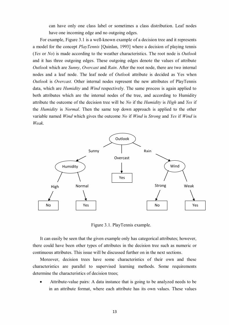
For example, Figure 3.1 is a well-known example of a decision tree and it represents
a model for the concept PlayTennis [Quinlan, 1993] where a decision of playing tennis
(Yes or No) is made according to the weather characteristics. The root node is Outlook
and it has three outgoing edges. These outgoing edges denote the values of attribute
Outlook which are Sunny, Overcast and Rain. After the root node, there are two internal
nodes and a leaf node. The leaf node of Outlook attribute is decided as Yes when
Outlook is Overcast. Other internal nodes represent the new attributes of PlayTennis
data, which are Humidity and Wind respectively. The same process is again applied to
both attributes which are the internal nodes of the tree, and according to Humidity
attribute the outcome of the decision tree will be No if the Humidity is High and Yes if
the Humidity is Normal. Then the same top down approach is applied to the other
variable named Wind which gives the outcome No if Wind is Strong and Yes if Wind is
Weak.
It can easily be seen that the given example only has categorical attributes; however,
there could have been other types of attributes in the decision tree such as numeric or
continuous attributes. This issue will be discussed further on in the next sections.
Moreover, decision trees have some characteristics of their own and these
characteristics are parallel to supervised learning methods. Some requirements
determine the characteristics of decision trees;
Attribute-value pairs: A data instance that is going to be analyzed needs to be
in an attribute format, where each attribute has its own values. These values
Outlook
Humidity
No
Yes
Wind
Yes
Yes
No
Sunny Rain
Overcast
Strong Weak Normal High
Figure 3.1. PlayTennis example.

14
can either be categorical or numeric. The same attribute cannot have different
values types in different data instances [Kantardzic, 2011].
Predefined output expectations: Every data instance that is going to be learned
from or that is going to be tested should be assigned a classification label or a
numeric output value.
Erroneous values: The training data might contain erroneous examples, but
decision trees can tolerate these errors. The error might be in attribute values or
in classification labels or continuous output values [Mitchell, 1997].
Missing values: The training data might contain missing data instance values,
but decision trees can tolerate these missing values as well. Similarly attribute
values, classification labels or continuous output values might be missing.
Sufficient data: A decision tree needs data like any other data mining method.
The number of training instances should be sufficient so that an effective and
robust tree construction could be done. The amount of test instances is also
very important in order to validate the accuracy of the decision tree
[Kantardzic, 2011]. Additionally, each class should have sufficient number of
instances to represent that class properly.
3.1. Univariate Decision Trees
Univariate by definition means involving one variate or variable quantity. Based on this
definition, it can be seen that choosing one attribute at a time to branch a tree node is
basically called univariate splitting. Continuing univariate branching while growing the
tree produces a univariate decision tree. Almost all of the commonly used decision tree
inducers and their splitting methods are constructed on the idea of univariate based tree
construction. The example in Figure 3.1 which was given to introduce the basic
structure of a decision tree was also in univariate form. The root node which was
Outlook had to make a three-way split since it had three attribute values, and the other
internal nodes also made splits in similar fashion. Additionally, constructing a decision
tree is usually a greedy method and is normally performed in a top down manner.
It would also be beneficial to explain branching types and the kind of attributes that
could be used when building a decision tree. There are basically three different
branching types [Han and Kamber, 2006];
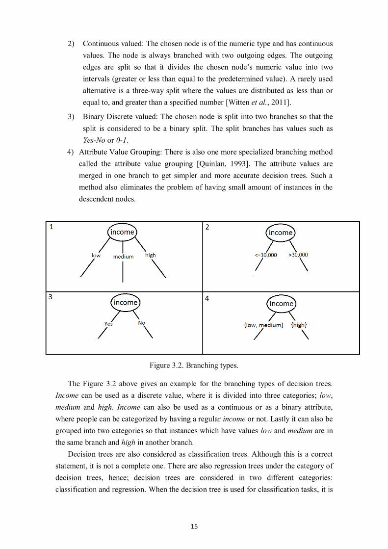
1) Discrete-valued: The chosen attribute in the decision tree induction is branched
so that all its categorical values (either ordinal or nominal) are used in their
own outgoing edges of the newly created node so that there is exactly one
branch for each attribute value. Basically, the node makes an n-way split
depending on the values of the node’s attribute where n denotes the number of
values the attribute has.
15
2) Continuous valued: The chosen node is of the numeric type and has continuous
values. The node is always branched with two outgoing edges. The outgoing
edges are split so that it divides the chosen node’s numeric value into two
intervals (greater or less than equal to the predetermined value). A rarely used
alternative is a three-way split where the values are distributed as less than or
equal to, and greater than a specified number [Witten et al., 2011].
3) Binary Discrete valued: The chosen node is split into two branches so that the
split is considered to be a binary split. The split branches has values such as
Yes-No or 0-1.
4) Attribute Value Grouping: There is also one more specialized branching method
called the attribute value grouping [Quinlan, 1993]. The attribute values are
merged in one branch to get simpler and more accurate decision trees. Such a
method also eliminates the problem of having small amount of instances in the
descendent nodes.
Figure 3.2. Branching types.
The Figure 3.2 above gives an example for the branching types of decision trees.
Income can be used as a discrete value, where it is divided into three categories; low,
medium and high. Income can also be used as a continuous or as a binary attribute,
where people can be categorized by having a regular income or not. Lastly it can also be
grouped into two categories so that instances which have values low and medium are in
the same branch and high in another branch.
Decision trees are also considered as classification trees. Although this is a correct
statement, it is not a complete one. There are also regression trees under the category of
decision trees, hence; decision trees are considered in two different categories:
classification and regression. When the decision tree is used for classification tasks, it is

16
called a classification tree and when it is used for regression tasks, it is referred to as a
regression tree [Rokach and Maimon, 2014].
Classification trees are designed for data which have finite number of class values.
The attributes can take numerical or categorical values. The main purpose of such kind
of trees is to classify the data to classification labels or classes by using classification
algorithms [Loh, 2011]. Splits of the tree or the goodness of the attributes are tested and
decided according to impurity measures. The attribute with the highest (or lowest
impurity) purity is chosen as the node to branch on. The main point for a purity measure
is to divide the attribute’s values into pure distributions of the classes. One of the mostly
used impurity measures is the entropy value [Quinlan, 1986] which will be discussed
later on.
The main idea behind the construction of a classification tree is fairly logical and
straightforward. It uses a top-down strategy and recursively splits starting from the root
node, where each node is branched according to the lowest impurity measure produced
amongst all other attributes. When there are no more splits available, the construction
stops.
One of the earliest classification trees was the concept learning system (CLS) [Hunt
et al., 1966]. Almost all of the other algorithms followed its approach including the ID3
algorithm which was found by Quinlan in 1979 [Quinlan, 1986]. The main idea of the
CLS was to begin with an empty decision tree and iteratively build the tree by adding
nodes until the tree classified all the training instances correctly. A pseudocode of the
CLS is given below [Hunt et al., 1966];
1. If all examples in the training instances in "C" are positive then create a node
called YES
If all examples in the training instances in "C" are negative then create a node
called NO
Otherwise, select and attribute A with values 𝑉1 ,𝑉2 , . . .𝑉𝑛 and create a
decision node
2. Partition the training examples in "C" into subsets 𝐶1,𝐶2, . . .𝐶𝑛 according to
the values of V.
3. Apply the algorithm to each of the sets in 𝐶𝑖 recursively.
Algorithm 1
The most popular and widely known inducers, for instance the C4.5 [Quinlan, 1993]
and CART [Breiman et al., 1984], they all use the same approach and even the most
recent inducers continue from the same path such as the C5.0 [Quinlan, 2004].
Regression trees are almost identical to classification trees; however, a regression
model has to be fitted to the algorithm. This means the aim of the tree is not
17
classification anymore, but it is regression. There are no more class labels or
classifications to make, instead the resulting leaf nodes of the tree are continuous values
which are used for prediction as well. Furthermore, entropy or similar measures cannot
be used as an impurity measure; mean squared error is used instead. Regression tree is
very similar to the classification trees and thus the same algorithm can be used by just
replacing the entropy measurements with mean squared errors calculations, and class
labels with averages [Alpaydin, 2014].
The only difference in the construction of a regression tree is the generation of leaf
nodes. These are generated by taking an average over the distributed target values of the
path that is taken after all the branching is done until that leaf node. Additionally, the
resulting tree is binary because the nodes are always branched into two partitions; some
value greater than or equal to, and a value less than the specified value. The algorithm
for constructing a regression tree is given below [Shalizi, 2009];
1. Start with single node containing all point values. Calculate the sum of squared
errors and prediction for leaves
2. If all the points in the node have the same value for all the input variables,
stop. Otherwise, search over all binary splits of all variables for the one which
will reduce sum of square errors (SSE) as much as possible. If the largest
decrease SSE would be less than some threshold or one of the resulting nodes
would contain less than some amount of points, stop. Otherwise, take that split,
creating two new nodes.
Algorithm 2
The first ever built regression tree is AID and it was built a couple of years before
THAID [Loh, 2011]. Both AID and CART follow a similar approach as Algorithm 2
which is a modified version of Algorithm 1.
3.1.1. Attribute Selection Criteria
Attribute selection is one of the fundamental properties of building a decision tree. The
selection of the attribute affects the entire decision tree since it will have an impact on
the efficiency and even the accuracy of the built tree. The aim is to generate a tree that
will efficiently and accurately classify the training data. The resulting model should be
as simple as possible which is also known as the Occam’s razor principle [Mitchell,
1997].
The main idea is based on purity and impurity in most of the cases. This means the
node that will be tested should be split into leaf or internal nodes (which are the values
of the tested attribute) that would be as pure as possible. The aim of purity is to partition
the data instances in training data so that the partitioned group (a leaf node or internal
18
node that a branch leads to from the tested node) would either have all or most of the
data instances in the same class category so that the entropy measure will be low [Han
and Kamber, 2006].
Additionally, commonly used decision trees are built as univariate decision trees;
therefore, the splitting criteria used in such trees are designed on top of univariate
factor. The following heuristic attribute selection methods are specifically used in
univariate trees: Information Gain, Gain Ratio, Gini Index, Twoing Criterion and Chi-
Squared criterion.
3.1.1.1. Information Gain
Information gain is one of the earliest and most commonly used decision tree attribute
selection criteria ever founded. Quinlan, who was the founder of the ID3 (Iterative
Dichotomiser 3) was also the first one who ever used information gain selection
criterion in a decision tree induction algorithm. However, without the concept of
entropy found by Claude E. Shannon [Shannon, 1951], information gain would not have
existed.
The criterion is based on top of information theory where the entropy measure plays
a key role. Entropy is the measure which tries to calculate the average amount of
information contained in each message received [Han et al., 2011]. In machine learning
terms, entropy tries to find the most valuable attribute that would be beneficial for a
model to be learnt.
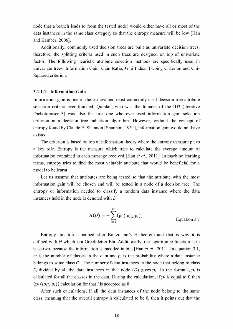
Let us assume that attributes are being tested so that the attribute with the most
information gain will be chosen and will be tested in a node of a decision tree. The
entropy or information needed to classify a random data instance where the data
instances held in the node is denoted with D.
𝐻 𝐷 = − p𝑖 (log2 p𝑖)
𝑚
𝑖=1
Equation 3.1
Entropy function is named after Boltzmann’s H-theorem and that is why it is
defined with H which is a Greek letter Eta. Additionally, the logarithmic function is in
base two, because the information is encoded in bits [Han et al., 2011]. In equation 3.1,
m is the number of classes in the data and 𝑝𝑖 is the probability where a data instance
belongs to some class 𝐶𝑖 . The number of data instances in the node that belong to class
𝐶𝑖 divided by all the data instances in that node (D) gives 𝑝𝑖 . In the formula, 𝑝𝑖 is
calculated for all the classes in the data. During the calculation, if 𝑝𝑖 is equal to 0 then
𝑝𝑖 (𝑙𝑜𝑔2 𝑝𝑖) calculation for that i is accepted as 0.
After such calculations, if all the data instances of the node belong to the same
class, meaning that the overall entropy is calculated to be 0, then it points out that the

19
node is totally pure and a leaf node can be formed. However, this is usually not the case,
so the calculations continue since the node is impure.
Now, if D is partitioned on an attribute A which can have categorical or numeric
values, it will either have n outcomes (attribute A’s values) or two outcomes if attribute
A is numeric. Let’s assume A is categorical; thus, the attribute A can split the existing D
into n partitions. Then, the expected information needed to classify a random data
instance when the attribute A is considered as root is calculated.
𝐻 𝐷|𝐴 = p(Aj)H(D|Aj
n
𝑗=1
Equation 3.2
The probability 𝑝(𝐴𝑗 ) is the relative frequency of the cases having 𝐴𝑗 over D. After
such a calculation, the overall entropy branching on the attribute A is found. The last
step is to calculate information gain for branching on the attribute A which is basically
subtracting the overall entropy of the attribute A from the original entropy calculation H
(D).
I(D|A) = H(D) − H(D|A)
Equation 3.3
Information gain in Equation 3.3 gives the gain that will be obtained after branching
on the attribute A. Therefore, information gain is calculated every time for every
possible attribute that can be branched on the test node to find the attribute which gives
the maximum information gain amongst the other attributes. The attribute with the
highest gain is branched on and the process continues until the classification is
completed.
3.1.1.2. Gain Ratio
Information Gain and Gini Index both favor attributes with many different values when
the attributes are tested because usually these attributes tend to have better entropy
calculations. This is because the more an attribute has values; it will have more chance
of turning its branches into a leaf node.
Quinlan uses the Gain Ratio attribute selection criterion in the C4.5 algorithm as an
update from ID3’s Information Gain method [Quinlan, 1993]. The only difference
between two attribute selection criteria is that Gain Ratio introduces a new
methodology; calculating the information on splitting attribute. By this normalization
method, the biased behavior is mostly eliminated.
𝐻 𝐴 = − p(Aj) log2 p(Aj)
n
𝑗=1
Equation 3.4
20
The calculation of split information on the splitting attribute is in fact an entropy
calculation. If the example given in Information Gain calculation is recalled, attribute A
was chosen as the test node and keeping that in mind, H(A) is denoted as the splitting
information of the attribute A in Equation 3.3. The probability of the value 𝐴𝑗 is simply
the relative frequency of that value.
GR D A =𝐼(𝐷|𝐴)
H(A)
Equation 3.5
When the Information Gain is calculated (which is exactly the same as in Equations
3.1-3.3), the information of that attribute is calculated next. Afterwards Information
Gain of the attribute is divided by the splitting information of the same attribute,
resulting in Gain Ratio. The attribute that has the highest Gain Ratio is chosen over the
rest of the tested attributes.
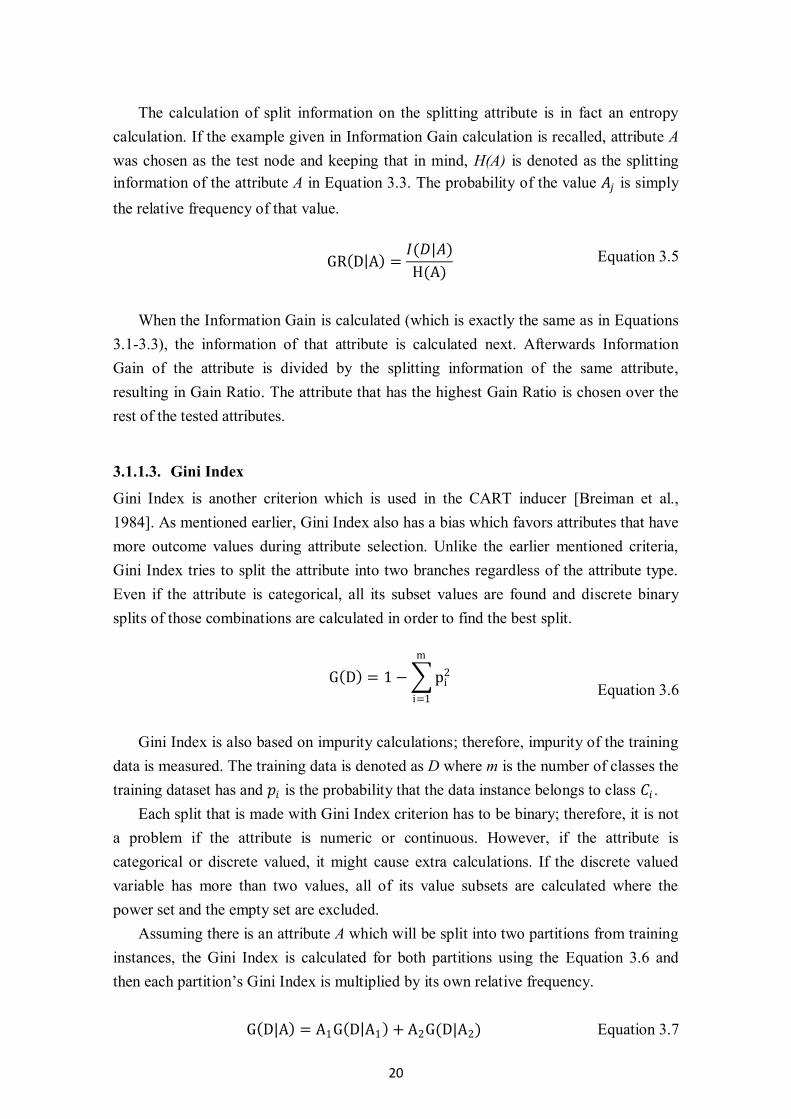
3.1.1.3. Gini Index
Gini Index is another criterion which is used in the CART inducer [Breiman et al.,
1984]. As mentioned earlier, Gini Index also has a bias which favors attributes that have
more outcome values during attribute selection. Unlike the earlier mentioned criteria,
Gini Index tries to split the attribute into two branches regardless of the attribute type.
Even if the attribute is categorical, all its subset values are found and discrete binary
splits of those combinations are calculated in order to find the best split.
G D = 1 − pi2
m
i=1
Equation 3.6
Gini Index is also based on impurity calculations; therefore, impurity of the training
data is measured. The training data is denoted as D where m is the number of classes the
training dataset has and 𝑝𝑖 is the probability that the data instance belongs to class 𝐶𝑖 .
Each split that is made with Gini Index criterion has to be binary; therefore, it is not
a problem if the attribute is numeric or continuous. However, if the attribute is
categorical or discrete valued, it might cause extra calculations. If the discrete valued
variable has more than two values, all of its value subsets are calculated where the
power set and the empty set are excluded.
Assuming there is an attribute A which will be split into two partitions from training
instances, the Gini Index is calculated for both partitions using the Equation 3.6 and
then each partition’s Gini Index is multiplied by its own relative frequency.
G D|A = A1G D A1 + A2G(D|A2)
Equation 3.7

21
The attribute which maximizes the difference between the initial Gini and the Gini
resulting after the split is chosen.
∆G D|A = G D − G(D|A)
Equation 3.8
3.1.1.4. Twoing Criterion
As in the case with Information Gain criterion, favoring test attributes which has wide
range of values is also an issue with Gini Index. Thus, the Twoing criterion is used in
the CART algorithm to overcome this bias [Rokach and Maimon, 2014].
T D A =P1P2
4[ |p A1,i − p A2,i |
m
i=1
]2
Equation 3.9
Assuming there is an attribute A which will be split into two partitions from training
instances D, P1 and P2 are the probabilities to get left or right nodes (binary nodes, first
node and second node). 𝑝 𝐴1,𝑖 and 𝑝 𝐴2,𝑖 are the probabilities of test node A’s first
and second partitions respectively where i is the given class. Gini Index and Twoing
work exactly the same when the target attribute is binary but when the target attribute is
multi valued, then Twoing criterion chooses attributes with evenly divided splits
[Rokach and Maimon, 2014]. This means Twoing criterion becomes biased as well
when the target attribute has more than two values. Lastly, Twoing criterion works
slower than the Gini Index resulting in efficiency loss [Kantardzic, 2011].
3.1.1.5. Chi-squared Criterion
Chi-squared criterion is used in CHAID inducer [Kass, 1980]. This criterion is used for
measuring the correlation between two attributes.
𝑋2 = (𝑥𝑗𝑖 − 𝐸𝑗𝑖 )2
𝐸𝑗𝑖
𝑚
𝑖
𝑛
𝑗
Equation 3.10
In Chi-squared criterion, split variables are decided based on the calculated p-values
[IBM, 2011]. If the attribute is categorical then Pearson Chi-square test is done
(Equation 3.10), if the attribute is continuous then an F test is made. The attribute with
smallest p-value is chosen amongst the ones that are computed and if it is greater than
the predetermined threshold, no further split is done along that branch and becomes a
leaf node. If the p-value is less than or equal to that predetermined threshold, the node is
split using the selected attribute. In the formula, 𝑥𝑗𝑖 is the frequency of the observed data
instances of attribute value j where the class that they belong is i. The expected

22
frequency of the data instances of attribute value j is denoted as 𝐸𝑗𝑖 where the class that
they belong is i. Equation 3.10 is for calculating the unadjusted p-value for categorical
attributes. Once the p-value is calculated, it can be adjusted by using the Bonferroni
adjustments. As a result, this criterion is based on observed and expected values where
frequency of the data instances classified in categories is essential.
3.1.1.6. Continuous Attribute Split
For numeric or continuous attributes, splitting is more or less the same as splitting a
categorical attribute. Information measure that will decide the goodness of the attribute
is obtained by the use of measures like; Information Gain, Gain Ratio, Gini Index.
However, the attribute values or possible split points are calculated differently since
continuous attributes do not have any predefined split values.
The commonly used technique is to find the middle point of each sorted adjacent
values in the dataset. This will result in (n-1) possible thresholds when there are n many
training instances [Maimon and Rokach, 2005]. Then these middle points become the
possible thresholds for a split. An information measure is calculated on every single
threshold that is found. Then, a threshold is selected amongst all according to the
calculated information measure. The split is made based on this threshold resulting in a
binary split.
The criteria that were introduced are used in commonly applied inducers both for
academic and business related purposes. The use and purpose of these univariate
splitting criteria are the same; however, all of them have different efficiency and
accuracy ratings on different kind of data sets. It is very hard to discuss which one has
better results by means of accuracy and efficiency since all these criteria are used in
different inducers and on different data sets most of the time. There are some researches
that have been made to find out which criterion results better in classifying a dataset in
terms of accuracy and Badulescu's article is one of them [Badulescu, 2007]. In the study
various attribute selection criteria (including Information Gain Ratio, Gini index, Chi-
squared criteria) have been tested. The error rates for Information gain ratio, Gini index
and Chi-squared criterion were respectively 13.41, 14.76 and 14.68. Therefore, it could
be considered that the findings have pointed out there is not much difference in terms of
accuracy between the commonly used attribute selection criteria. However, Information
Gain Ratio has outperformed the other criterion during these tests which were made by
using 29 different attribute selection measures [Badulescu, 2007].
3.1.2. Pruning Methods
One of the most important factors that are directly related with decision tree
accuracy is pruning. Pruning by definition is basically eliminating the subtrees and
replacing them with leaf nodes so that the performance of the tree can improve in terms

23
of accuracy and efficiency on unseen cases. One main reason why pruning is essential
lies behind the rule of Occam’s razor; “Among competing hypotheses, the one with the
fewest assumptions should be selected [Blumer et al., 1987].” This notion is very
accurate when the tree is overfitted. When the tree is overfitted, it becomes a tree model
with too much bias on the training data since it is purely grown out of the training data.
Hence, test data is needed to measure accuracy of the tree on new unseen cases and
prune the tree accordingly [Kantardzic, 2011]. The scientific studies have shown that
pruning can have crucial effect on decision tree accuracy [Mingers, 1989]. According to
another study, it has been shown that pruning can affect the accuracy up to 50% within
considerable confidence intervals [Frank, 2000].
Figure 3.3. Post-pruning example [Han et al., 2011].
An example of pruning is given above in Figure 3.3. As mentioned, pruning is
eliminating subtrees (𝐴3) and turning them into leaf nodes (class B). This shows the
significance of pruning even though the tree size is small. Now, if the tree becomes
larger than this (in which almost all of the data mining practices the tree size is much
larger than the tree in the figure), the significance of pruning becomes even more
important. It is because as the tree grows bigger, it becomes more complex and harder
to handle which also affects the accuracy because of overfitting. The accuracy is
affected because when the tree is too large or too complex the noisy or exceptional
cases can be included in the model and this action would lead to misclassification errors
[Tan et al., 2006]. Additionally, as the tree grows larger the subtrees grow larger with
the tree, producing more paths that lead to more and different classifications which can
lead to misclassification results in the end.
There are two different pruning approaches; prepruning and postpruning. In
prepruning, a decision tree is halted while growing so that it won’t get too complex.
24
However, in postpruning the tree is grown till its fullest and then pruned following a
bottom up or a top down strategy.
The tree that has been grown fully or, in other words, that have overfitted might not
be successful in classifying test cases. On the other hand, a tree that is not grown
adequately might not be enough to be a sufficient decision tree model and this would
result in unsuccessful classifications on the test data. Therefore, trying to find a
common solution that knows where and when to stop growing the tree is very hard and
is known as the horizon effect [Frank, 2000].
Prepruning is considered as a more interesting method because it would save time
since no time would be wasted growing subtrees that will be eliminated further on
[Witten et al., 2011]. Actually trees are not pruned in prepruning algorithms; instead
the algorithms are halted due to some stopping criterion. This criterion is usually based
on goodness of the split. As discussed earlier, decision trees need splitting criterion such
as Information Gain, Gini Index, Gain Ratio and so on to determine which attribute to
branch on. If the information measured at a test node is under some threshold that is
defined earlier, then the branching is halted on that path. Another prepruning strategy is
limiting the tree size and the instances in an internal node to some user-specific
threshold. Lastly, if a class distribution of instances is independent of the available
feature, the tree growing is halted. Thus, it can easily be concluded that prepruning is
based on restrictive conditions which are controlled by some threshold values.
Postpruning on the other hand is not restricted by thresholds. The tree is grown
entirely until it cannot grow anymore and then trimmed so that it gives better accuracy
on the test data. There are two major operations in postpruning; subtree replacement and
subtree raising [Witten et al., 2011]. Subtree replacement is the basic element of
pruning where the subtree is replaced with a leaf node. This operation might lower the
accuracy in the training data; however, it will increase the accuracy in the test data. The
other operation is subtree raising which is more complicated than subtree replacement
and is used in C4.5 inducer. The subtree on a path of the tree is pruned but replaced by
another subtree which has different leaf nodes and gives better accuracy. The new
subtree which replaces the old one is grown which means that subtree raising requires a
lot of time and it is a complex operation. One last important point of postpruning is
when the subtree is pruned and replaced with a leaf node, the criteria of labeling is the
frequency of instances in that subtree; the most frequent class is labeled as the leaf node
class after pruning [Han et al., 2011].
If pre and postpruning are compared, prepruning gives better efficiency since it halts
the tree growing which means producing trees faster; however, postpruning gives better
accuracy in overall according to most of the studies [Alpaydin, 2014]. One of the
reasons for postpruning giving better accuracy is the so called interaction effect; in
prepruning each attribute is evaluated individually before being pruned which means
neglecting the reactions between those attributes which might be important by terms of

25
accuracy [Frank, 2000]. Postpruning solves this issue since all possible attribute paths
and interactions are seen clearly in the fully grown tree. Therefore, postpruning is the
most widely used technique in pruning and some most important postpruning
algorithms are; cost-complexity pruning, minimum-error pruning, reduced error
pruning, pessimistic pruning and error based pruning.
3.1.2.1. Cost Complexity Pruning
Cost complexity pruning which is also referred to as the weakest link pruning is used in
CART [Breiman et al., 1993] inducer and it consists of two parts. In the first part, a
sequence of trees is built by training data. Each tree in the sequence is built so that the
succeeding tree is obtained by pruning one or more subtrees in the preceding tree where
the first tree of the sequence is the unpruned tree and the last of the sequence is the same
tree with only the root remaining. Subtrees are pruned according to their sizes in which
relatively have the smallest increases in their error rate on the training data. An error
rate 𝛼 is calculated by subtracting the error rate of the pruned tree from the initial tree
and then dividing it by the number of leaf difference between the initial and pruned
trees.
In the second part of the algorithm, one optimal tree is chosen from the sequence of
trees. In order to choose the optimal tree, generalization error of each and every pruned
tree is calculated so that the tree with the least generalization error is chosen. The
generalization error is estimated either by employing holdout method or cross validation
method.
Cost complexity pruning usually performs well in terms of accuracy; however, the
same statement cannot be made for its efficiency. The algorithm performs in quadratic
time since a sequence of pruned decision trees are being obtained and checked for
generalization errors which requires heavy time complexity [Frank, 2000]. Furthermore,
there were several issues with cost complexity pruning according to Quinlan [Quinlan,
1987]. The first problem was that it was unclear why cost complexity pruning method
was “superior to other possible models such as the product of error rate and number of
leaves.” Additionally, “it seems anomalous that the cost-complexity model used to
generate the sequence of subtrees is abandoned when the best tree is selected.”
Therefore, he would later on find new pruning algorithms; reduced error pruning and
pessimistic pruning which would aim to solve these problems and eventually lead to
another algorithm called error based pruning.
3.1.2.2. Reduced Error Pruning
This pruning algorithm suggested by Quinlan is a rather straightforward and simple
method [Quinlan, 1987]. The method follows a bottom up strategy where a fully grown
tree is pruned starting from the bottom-most non-leaf nodes. Then the algorithm checks
26
each internal node and replaces the node with the most popular classification category
(class label). The node to be replaced is chosen according to the number of errors it
produces when the subtree is kept as it is and when it is replaced with the most
frequently occurring class. The number of errors are calculated by using a separate test
set. If the number of errors increases when the subtree is pruned, then the subtree is
kept, otherwise pruned. The node with the most gain is pruned amongst all the other
internal nodes. The algorithm continues its recursion until the error calculated on the
nodes to be pruned makes no difference or does not improve tree accuracy.
3.1.2.3. Pessimistic Pruning
Pessimistic pruning is the other pruning algorithm suggested by Quinlan. The most
interesting point of this method is it does not need a separate pruning or test data to
employ the pruning algorithm [Quinlan, 1987]. It aims to improve the error rate
calculated when unseen data are classified. The key idea in the algorithm is to make an
assumption that ½ of an instance in leaf nodes of the trained subtree is going to be
classified incorrectly in addition to the already misclassified number of instances on that
subtree when unseen cases are encountered. This constant is obtained by using the
“continuity correction” for the binomial distribution [Quinlan, 1987].
The methodology is closely related with reduced error pruning such that it also tries
to replace subtrees with the most frequent classification in the data. It starts by
performing a top down traversal over the tree instead of a bottom up approach. All the
internal nodes are traversed recursively and pruned if the number of errors
(misclassified cases in the node) + ½ is within one standard error of the earlier
estimated number of errors in the subtree. If the internal node is pruned, its subtrees are
not checked for pruning.
According to Quinlan, this method has two advantages. Firstly, it is much faster
than cost complexity pruning and reduced error pruning since a sequence of trees is not
produced where almost all the same subtrees are traversed each time. Instead, only one
tree is taken into consideration and each subtree is examined at most once. The second
advantage is there is no need for a separate testing data to employ the pruning
algorithm; only training data is enough.
3.1.2.4. Minimum Error Pruning
Minimum error pruning was first introduced by Niblett and Bratko in 1986 [Niblett and
Bratko, 1987]. Its main objective is to prune the tree by the help of most frequent class
label.
The algorithm's aim is to find an expected error rate when it is predicted that all the
future examples will be in class c. The predicted or expected error rate is given in
Equation 3.11 where n is the total number of training instances, 𝑛𝑐 is the number of

27
instances in the most frequent class and k is the number of classes in the data [Mingers,
1989]. Algorithm first calculates the expected error rate at each internal node if that
subtree is pruned. Then calculates the expected error rate if the node is not pruned,
combined with weighting according to the proportion of observations along each
branch. If pruning the node gives a higher expected error rate, then the subtree is kept
otherwise pruned. These calculations continue recursively until the tree is totally pruned
according to the stopping criteria.
𝐸𝑘 =(𝑛 − 𝑛𝑐 − 𝑘 − 1)
𝑛 + 𝑘
Equation 3.11
It is also very similar to reduced error pruning because it also follows a bottom up
approach and prunes the tree if the error rate is more than the unpruned version of it.
The algorithm assumes that all classes are equally likely which is actually a
disadvantage, because in practice the classes are not equally likely so the results
obtained on practice becomes worse than expected.
3.1.2.5. Error Based Pruning
Error based pruning is basically a more complicated version of pessimistic pruning with
some important updates. It is used in the well known decision tree inducer C4.5. Both
error based pruning and C4.5 were introduced by Quinlan [Quinlan, 1993]. Like
pessimistic pruning, it does not require a separate pruning data to prune the tree.
However, unlike pessimistic pruning but similar to reduced error pruning, a bottom up
traversal is employed in the algorithm. The other important aspect of the algorithm is
that it provides subtree raising methodology in addition to subtree replacement and
combines them in one algorithm.
It estimates the errors as if the errors are binomially distributed like in pessimistic
pruning. Instead of having a standard error rule, it introduces a confidence interval on
the error counts which is 25% by default. The leaves’ error rates are calculated by
taking the confidence interval’s upper bound.
The algorithm works from bottom to up and estimates errors for 3 different cases
[Rokach and Maimon, 2014];
1) The overall error rate of the tree when node N does not prune its subtree
2) The overall error rate of the tree when node N prunes its subtree
3) The overall error rate of the tree when the node N’s subtree is pruned by
replacing the whole subtree with its most frequently used child node.
According to the error rate obtained, the option that has the lowest value is chosen
which means either the subtree is replaced with a leaf node or not. The last option is
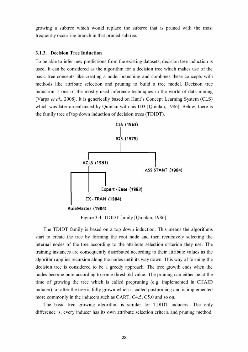
28
growing a subtree which would replace the subtree that is pruned with the most
frequently occurring branch in that pruned subtree.
3.1.3. Decision Tree Induction
To be able to infer new predictions from the existing datasets, decision tree induction is
used. It can be considered as the algorithm for a decision tree which makes use of the
basic tree concepts like creating a node, branching and combines these concepts with
methods like attribute selection and pruning to build a tree model. Decision tree
induction is one of the mostly used inference techniques in the world of data mining
[Varpa et al., 2008]. It is generically based on Hunt’s Concept Learning System (CLS)
which was later on enhanced by Quinlan with his ID3 [Quinlan, 1986]. Below, there is
the family tree of top down induction of decision trees (TDIDT).
Figure 3.4. TDIDT family [Quinlan, 1986].
The TDIDT family is based on a top down induction. This means the algorithms
start to create the tree by forming the root node and then recursively selecting the
internal nodes of the tree according to the attribute selection criterion they use. The
training instances are consequently distributed according to their attribute values as the
algorithm applies recursion along the nodes until its way down. This way of forming the
decision tree is considered to be a greedy approach. The tree growth ends when the
nodes become pure according to some threshold value. The pruning can either be at the
time of growing the tree which is called prepruning (e.g. implemented in CHAID
inducer), or after the tree is fully grown which is called postpruning and is implemented
more commonly in the inducers such as CART, C4.5, C5.0 and so on.
The basic tree growing algorithm is similar for TDIDT inducers. The only
difference is, every inducer has its own attribute selection criteria and pruning method.
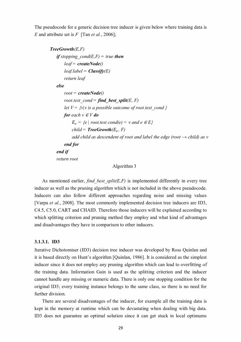
29
The pseudocode for a generic decision tree inducer is given below where training data is
E and attribute set is F [Tan et al., 2006];
TreeGrowth(E,F)
if stopping_cond(E,F) = true then
leaf = createNode()
leaf.label = Classify(E)
return leaf
else
root = createNode()
root.test_cond = find_best_split(E, F)
let V = {v|v is a possible outcome of root.test_cond }
for each v ∈ V do
𝐸𝑣 = {e | root.test cond(e) = v and e ∈ E}
child = TreeGrowth(𝐸𝑣 , F)
add child as descendent of root and label the edge (root → child) as v
end for
end if
return root
Algorithm 3
As mentioned earlier, find_best_split(E,F) is implemented differently in every tree
inducer as well as the pruning algorithm which is not included in the above pseudocode.
Inducers can also follow different approaches regarding noise and missing values
[Varpa et al., 2008]. The most commonly implemented decision tree inducers are ID3,
C4.5, C5.0, CART and CHAID. Therefore those inducers will be explained according to
which splitting criterion and pruning method they employ and what kind of advantages
and disadvantages they have in comparison to other inducers.
3.1.3.1. ID3
Iterative Dichotomiser (ID3) decision tree inducer was developed by Ross Quinlan and
it is based directly on Hunt’s algorithm [Quinlan, 1986]. It is considered as the simplest
inducer since it does not employ any pruning algorithm which can lead to overfitting of
the training data. Information Gain is used as the splitting criterion and the inducer
cannot handle any missing or numeric data. There is only one stopping condition for the
original ID3; every training instance belongs to the same class, so there is no need for
further division.
There are several disadvantages of the inducer, for example all the training data is
kept in the memory at runtime which can be devastating when dealing with big data.
ID3 does not guarantee an optimal solution since it can get stuck in local optimums
30
because it uses greedy strategy [Rokach and Maimon, 2014]. As mentioned earlier it
can overfit the data since it does not employ any pruning algorithm on its own.
Additionally, numeric or continuous data cannot be used directly in this inducer; it
should be converted into a categorical attribute before being used. Lastly, Information
Gain criteria can be biased on multiple valued attributes so it may not choose the best
greedy path on all times.
3.1.3.2. C4.5
C4.5 is considered as an evolved ID3. Quinlan targeted ID3’s weaknesses and made a
better inducer which is more efficient and accurate [Quinlan, 1993]. Gain Ratio is used
to overcome the bias of the earlier Information Gain criterion. It performs postpruning
by the help of error based pruning algorithm. Continuous and numeric data can be used
in C4.5 and it can also handle missing values. The growing algorithm stops when;
Every training instance belongs to the same class.
None of the remaining attributes provide better Information Gain.
There are no training instances in a node.
There are some very important enhancements on the existing ID3 algorithm. One of
them is attribute value grouping; attributes values are also tested as a group and
compared with all the other possible combinations of existing attribute values so that it
gives better Gain Ratio in order to be selected. As mentioned earlier, C4.5 can handle
missing values. The inducer accomplishes such a task by giving the option to mark the
missing values with “?” so that those missing values are handled in a probabilistic way
in decision tree construction. Another important enhancement is pruning. Error based
pruning gives a more pessimistic approach than pessimistic pruning which enables C4.5
to increase its accuracy and become more robust against noise. Additionally, subtree
raising feature is also implemented so that C4.5 not only prunes a branch from the tree
but it can also grow one that replaces the pruned branch. Error based pruning gives a
well overall accuracy and avoids the constructed tree from overfitting the training data
unlike ID3. The other important improvement is that the inducer can now use the
continuous attributes without converting them into categorical attributes. Instead it
marks each middle point of existing ordered or sorted attribute values as a possible
interval threshold and tests those intervals according to their Gain Ratio. The interval
with the highest Gain Ratio is then branched using a binary split. One downfall that
seems to be unresolved is the memory usage; the inducer keeps all the training data in
the runtime memory which results in poor efficiency.
31
3.1.3.3. C5.0
C5.0 in UNIX or See5 in Windows operating system is the successor of C4.5 [Quinlan,
2004]. It is a commercially used inducer; however, the single threaded version of the
inducer has been made public for personal or research related use only. C5.0 is much
more efficient than the predecessor C4.5 by means of computational power and memory
management [Rokach and Maimon, 2014]. A classification task that is completed in one
and a half hour with C4.5 can be completed in three and a half seconds with C5.0
inducer [Rokach and Maimon, 2014].
The tree is constructed again in a top down recursive and greedy manner. It is still
using postpruning methodology to avoid overfitting. An enhanced version of error
based pruning is implemented where again the confidence interval can be defined. Gain
Ratio and Information Gain are still the attribute selection criteria used in the inducer.
Nonetheless, there are some improvements over the C4.5 inducer [Quinlan, 2004];
A variant of boosting is implemented which increases the prediction accuracy
dramatically.
New data types such as dates, time, timestamps, “not applicable” values,
attribute misclassification costs and some attribute prefiltering functions.
The generated decision trees are smaller, more appropriate for Occam’s razor.
Speed and memory usage as mentioned earlier.
Each case instance can be weighted; giving it more importance over other
cases.
Generates less number of rules.
Can cope with dimensionality by winnowing.
3.1.3.4. CART
Classification and regression trees (CART) is another inducer found by [Breiman et al.,
1984]. The inducer algorithm also follows a top down greedy approach which
recursively grows the tree. It is different from the earlier mentioned inducers such that
it splits the attributes in binary no matter how many values the attribute has. This seems
like an advantage at first since there will not be the negative consequences of multi way
splits; however, the same attribute can be branched on different values of its own at the
proceeding levels of the tree which may produce a less interpretable and unnecessarily
long tree. The first version of the algorithm uses Gini Index for attribute selection
criteria but it is later on replaced by Twoing criteria since Gini Index tends to favor
attributes with more values. The reason Gini Index was chosen in the first place was
because it was thought that Gini Index gave better performance by terms of speed than
the Information Gain when it came to attribute selection [Kantardzic, 2011].

32
The pruning method chosen for the CART inducer is cost complexity pruning.
Hence, the pruning is supported by cross validation method where other inducers are
not such as C5.0 where a single-pass algorithm is derived from binomial confidence
limits [Hssina et al., 2014]. Another important difference that separates it from the other
inducers is that it looks for a possible solution that approximates the results when the
attribute has an unknown value. Lastly, CART inducer supports regression based
induction which is important since at the time it was introduced it was one of the most
accurate inducers which can employ regression by using least-squared error
methodology.
3.1.3.5. CHAID
Chi-squared automatic interaction detection (CHAID) is also another important inducer
that differently follows the THAID which is another classification tree algorithm. It is
mostly used for research purposes and in the industry for direct marketing because it is
fast and supports both classification and regression. It is one of the first successful
decision trees introduced by Gordon Kass in 1980 [Kass, 1980]. It was first used for
classifying nominal values only but later on it was adapted for other kind of attributes as
well. It uses F test for the continuous attributes, Pearson chi-square test for nominal and
likelihood ratio test for the ordinal attributes [Rokach and Maimon, 2014].
The inducer does not have a pruning algorithm. An interesting aspect of the
algorithm is that it treats the missing values as instances of the same category. CHAID
makes a multiway split for the tested attributes and needs large training data to work
effectively. During the splits each attribute is branched so that the children have
homogeneous values of the selected attributes. Additionally, the splits are made based
on a predefined threshold such that if the threshold is not met, the inducer will not
branch and it will stop. Some other stopping conditions are as follows;
Predefined tree depth is reached.
A threshold for being a parent node is reached in terms of instances the node
has.
A threshold for being child node is reached in terms of instances the node has.
3.1.4. Rule sets
Rules in general are very good ways to express knowledge or represent information
acquired from a plain or mined data set. In association rule mining, inferences are made
from data and expressed as rule sets. Nonetheless, another use for rules exists in
decision trees.
One of the reasons decision trees are preferred is because of their simplicity in
interpreting the results of the processed dataset. However, in most real world cases

33
decision trees can grow into very big and complex structures which make them hard to
interpret even though they might have been pruned [Han et al., 2011]. Therefore, rules
come in handy in such cases where the trees are simplified into IF-THEN rules which
are referred to as decision rules.
An IF-THEN rule is an expression in the form; IF condition THEN conclusion. The
“IF” part or the left hand side of a rule is called the rule antecedent or precondition. The
“THEN” part or the right hand side of a rule is called the rule consequent. The
consequent of the rule withholds the classification label or the prediction of that rule
[Han and Kamber, 2006]. Extracting rules from a grown decision tree is very
straightforward. Each extracted rule is basically the path from the root to a leaf node. To
extract rules, each split attribute is “ANDed” to the “IF” part of the rule according to its
value until the leaf node is reached which forms the consequent or the “THEN” part of
the rule.
The rules that are extracted are mutually exclusive and exhaustive since they are
directly extracted from the tree. There is a disjunction or “OR” implication between the
rules that are extracted which supports the idea of mutually exclusiveness. This also
means the rules cannot overlap or conflict with each other since the extracted rules
match the leaves of the tree in a one on one relationship. Exhaustive term means that
there is a rule for each training case (for each attribute-value combination occurring in
the tree) .
A rule set or decision rules can be pruned like a decision tree as well. Sometimes
the rules or parts of them can be useless or do not have proper decision tree accuracy
since the rules might have been extracted from an unpruned tree. In this case, the rules
are pruned according to some pruning algorithm. For example, C4.5 algorithm has a
feature where it produces decision rules as well as a decision tree and prunes the rules
using error based pruning. A consequence of rule pruning might be losing mutually
exclusiveness property since after pruning, there will not be any guarantee that each
possible path will go to a separate leaf node. However, this conflict can be handled just
like Quinlan has done in C4.5 by adapting a class-based ordering scheme [Han et al.,
2011]. It groups rules for a single class together and then determines a ranking of these
class rule sets.
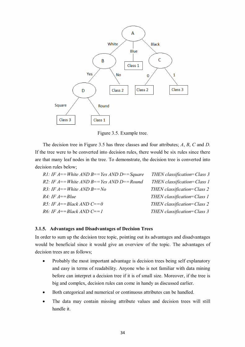
34
Figure 3.5. Example tree.
The decision tree in Figure 3.5 has three classes and four attributes; A, B, C and D.
If the tree were to be converted into decision rules, there would be six rules since there
are that many leaf nodes in the tree. To demonstrate, the decision tree is converted into
decision rules below;
R1: IF A==White AND B==Yes AND D==Square THEN classification=Class 3
R2: IF A==White AND B==Yes AND D==Round THEN classification=Class 1
R3: IF A==White AND B==No THEN classification=Class 2
R4: IF A==Blue THEN classification=Class 1
R5: IF A==Black AND C==0 THEN classification=Class 2
R6: IF A==Black AND C==1 THEN classification=Class 3
3.1.5. Advantages and Disadvantages of Decision Trees
In order to sum up the decision tree topic, pointing out its advantages and disadvantages
would be beneficial since it would give an overview of the topic. The advantages of
decision trees are as follows;
Probably the most important advantage is decision trees being self explanatory
and easy in terms of readability. Anyone who is not familiar with data mining
before can interpret a decision tree if it is of small size. Moreover, if the tree is
big and complex, decision rules can come in handy as discussed earlier.
Both categorical and numerical or continuous attributes can be handled.
The data may contain missing attribute values and decision trees will still
handle it.

35
The data might have error and decision trees will still handle it. They are robust
to noise.
It follows a nonparametric approach; therefore, it does not require any prior
assumptions regarding the type of distributions satisfied by the class and other
attributes [Tan et al., 2006].
Constructing decision trees are computationally inexpensive and fast which
enables constructing models that require large sized training datasets to be
easier, computationally inexpensive (in comparison with other machine
learning algorithms) and faster [Maimon and Rokach, 2005].
Decision tree representation is rich enough to represent any discrete values
classifier [Rokach and Maimon, 2014].
Decision trees can handle high dimensional data [Iltanen, 2014].
Decision trees can handle heterogeneous data [Iltanen, 2014].
Some of the disadvantages of decision trees are as follows;
Big majority of the inducers require the target value of the data instances to be
discrete valued only.
A subtree can be replicated many times in a decision tree because tree is
constructed in a divide and conquer manner (each subtree constructed is
independent) [Tan et al., 2006]. A decision tree cannot represent the same
subtrees as one so it will replicate the trees since every path is mutually
exclusive [Rokach and Maimon, 2014].
Since decision trees are greedy, they sometimes become overly sensitive and
tend to choose a split due to a noise or an irrelevant attribute. This would cause
all the subtrees of that split to change which would result in a wrong split and
affect the accuracy poorly.
Decision trees are greedy and recursive which results in decreasing the number
of instances and scattering them among nodes as the tree grows downwards.
When the leaf nodes are reached, sometimes the number of data instances that
is remaining for the leaf node might be very small. This would mean that the
remaining instances are not sufficient to make a statistically significant
decision for the class representation of the nodes [Tan et al., 2006]. This is also
known as the data fragmentation problem.
It is true that decision trees can handle missing values but this also has a
disadvantage. Handling the missing data require a lot of computation which is a
drawback by means of computational time [Rokach and Maimon, 2014].

36
A decision tree inducer mostly follows a univariate approach; therefore, these
inducers check one attribute at a time. This strategy divides the attribute space
into regions. The borders between two neighboring regions that belong to
different classes are called decision boundaries and these boundaries are
rectangular. Hence, this fact limits the expressiveness of the tree and withdraws
it from modeling complex relationships among continuous attributes. There are
some techniques such as oblique decision tree method and constructive
induction method but these methods are proven to be time consuming and
expensive by means of computation [Tan et al., 2006].
3.2. Multivariate decision trees
As mentioned earlier, univariate by definition means involving one variate or variable
quantity. On the other hand, multivariate means using multiple or more than one variate
or variable quantity at the same time. Therefore, multivariate decision trees can use use
all attributes at one node when branching [Alpaydin, 2014].
Hyperplanes with an arbitrary orientation are used [Kantardzic, 2011] in
multivariate trees. It means that there can be 2𝑑 𝑁𝑑 possible Hyperplanes (where d is
the number of dimensions and N is the number of possible thresholds for the split
points) which makes exhaustive search inefficient and impractical. Consequently, a
more practical way to follow is using linear multivariate node that takes weights for
each attribute and sums them up [Alpaydin, 2014]. Moreover, linear multivariate
decision trees choose the most important attributes amongst all so that the process
would become more efficient and practical.
Several decision tree inducers have been proposed according to multivariate
approach. One of the earliest examples was the CART algorithm. It would decrease the
dimensionality in the data preprocessing session to reduce the complexity at each node.
After the preprocessing, the inducer used multivariate approach by adjusting the
weights of the attributes one by one.
As a result, it can be said that multivariate decision trees are used to do a better
classification and approximation by the help of hyperplanes. However, this process is
very complex and time consuming which also requires more data than univariate trees
to bring optimal results.

37
4. Evaluation of Decision Trees
At the time a model is built for a decision tree, the first question that comes into mind is
how accurate or reliable the model is on unseen cases. This is the reason why evaluation
of decision trees is essential because one should be certain that the resulting decision
tree will be reliable and efficient. In some cases, there might be more than one decision
tree model for a specific machine learning problem and one of them must be preferred
over the others. In such cases, the only option to overcome such a problem is to take
some precautionary steps. This is achieved by using measures and metrics that will
estimate the overall performance of the inducer’s model for future use.
In this section, the most common and efficient metrics that are necessary for
decision trees are going to be discussed and some important questions will be answered.
What are some common metrics for estimating decision tree performance? What is
accuracy? What are other measures for decision tree evaluation? After discussing such
questions, widely used accuracy estimation methodologies will be discussed.
4.1. Performance Evaluation Metrics and Measures
Before discussing what kind of measures there are, the type of metrics that are used for
performance evaluation need to be explained. A metric for decision tree performance
can have various different meanings. In some cases, the performance is measured by
speed, sometimes by the size of the grown tree and in most cases it is measured by
accuracy. Below are some metrics that have been considered viable and their
definitions. [Han et al., 2011]
Accuracy Based: These are various measures that show the performance of
classifiers on rating systems or percentages. Accuracy based metrics have
dominated the evaluation methods and techniques since they give the most
realistic and easily calculable results. Some of them are accuracy (recognition
rate), error rate, recall, specificity and precision.
Speed: It is usually referred as the computational costs that are encountered
during building the model and using it afterwards.
Robustness: This is how reliable or correct predictions a classifier makes when
it encounters noisy data or data with missing values.
Scalability: This can be considered as an aspect to evaluate when the classifier
is given large amounts of data. It measures how well the classifier operates
given the large amount of data and is usually evaluated by classifying data of
increasing size.
Interpretability: The amount or extent where the results of the classifier can
be interpreted. This is a measurement where it can be very hard to assess
different classifiers based on it since it is subjective. As mentioned earlier,
interpretability of decision trees can be easy until some point; however, it is
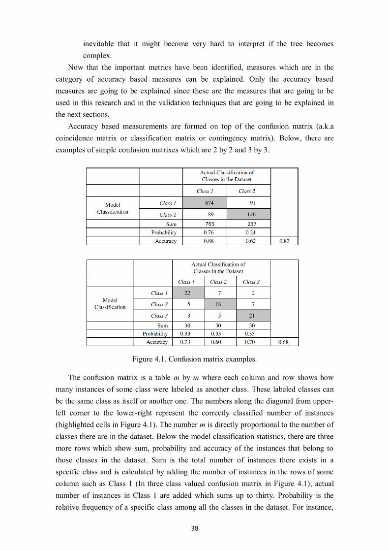
38
inevitable that it might become very hard to interpret if the tree becomes
complex.
Now that the important metrics have been identified, measures which are in the
category of accuracy based measures can be explained. Only the accuracy based
measures are going to be explained since these are the measures that are going to be
used in this research and in the validation techniques that are going to be explained in
the next sections.
Accuracy based measurements are formed on top of the confusion matrix (a.k.a
coincidence matrix or classification matrix or contingency matrix). Below, there are
examples of simple confusion matrixes which are 2 by 2 and 3 by 3.
Figure 4.1. Confusion matrix examples.
The confusion matrix is a table m by m where each column and row shows how
many instances of some class were labeled as another class. These labeled classes can
be the same class as itself or another one. The numbers along the diagonal from upper-
left corner to the lower-right represent the correctly classified number of instances
(highlighted cells in Figure 4.1). The number m is directly proportional to the number of
classes there are in the dataset. Below the model classification statistics, there are three
more rows which show sum, probability and accuracy of the instances that belong to
those classes in the dataset. Sum is the total number of instances there exists in a
specific class and is calculated by adding the number of instances in the rows of some
column such as Class 1 (In three class valued confusion matrix in Figure 4.1); actual
number of instances in Class 1 are added which sums up to thirty. Probability is the
relative frequency of a specific class among all the classes in the dataset. For instance,
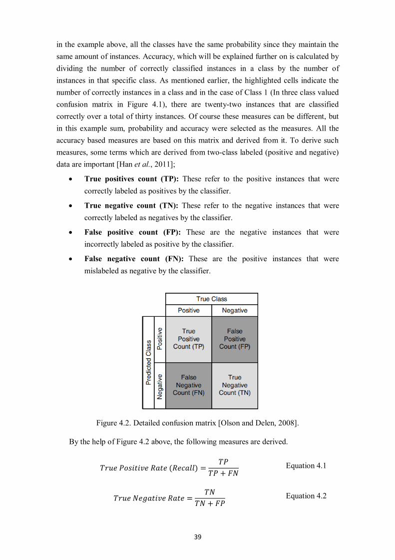
39
in the example above, all the classes have the same probability since they maintain the
same amount of instances. Accuracy, which will be explained further on is calculated by
dividing the number of correctly classified instances in a class by the number of
instances in that specific class. As mentioned earlier, the highlighted cells indicate the
number of correctly instances in a class and in the case of Class 1 (In three class valued
confusion matrix in Figure 4.1), there are twenty-two instances that are classified
correctly over a total of thirty instances. Of course these measures can be different, but
in this example sum, probability and accuracy were selected as the measures. All the
accuracy based measures are based on this matrix and derived from it. To derive such
measures, some terms which are derived from two-class labeled (positive and negative)
data are important [Han et al., 2011];
True positives count (TP): These refer to the positive instances that were
correctly labeled as positives by the classifier.
True negative count (TN): These refer to the negative instances that were
correctly labeled as negatives by the classifier.
False positive count (FP): These are the negative instances that were
incorrectly labeled as positive by the classifier.
False negative count (FN): These are the positive instances that were
mislabeled as negative by the classifier.
Figure 4.2. Detailed confusion matrix [Olson and Delen, 2008].
By the help of Figure 4.2 above, the following measures are derived.
𝑇𝑟𝑢𝑒 𝑃𝑜𝑠𝑖𝑡𝑖𝑣𝑒 𝑅𝑎𝑡𝑒 (𝑅𝑒𝑐𝑎𝑙𝑙) =𝑇𝑃
𝑇𝑃 + 𝐹𝑁
Equation 4.1
𝑇𝑟𝑢𝑒 𝑁𝑒𝑔𝑎𝑡𝑖𝑣𝑒 𝑅𝑎𝑡𝑒 =𝑇𝑁
𝑇𝑁 + 𝐹𝑃
Equation 4.2

40
𝐴𝑐𝑐𝑢𝑟𝑎𝑐𝑦 =𝑇𝑃 + 𝑇𝑁
𝑇𝑃 + 𝑇𝑁 + 𝐹𝑃 + 𝐹𝑁
Equation 4.3
𝑃𝑟𝑒𝑐𝑖𝑠𝑖𝑜𝑛 =𝑇𝑃
𝑇𝑃 + 𝐹𝑃
Equation 4.4
𝐹 𝑀𝑒𝑎𝑠𝑢𝑟𝑒 =2
1𝑃𝑟𝑒𝑐𝑖𝑠𝑖𝑜𝑛 +
1𝑅𝑒𝑐𝑎𝑙𝑙
Equation 4.5
The true positive rate (also known as hit rate or recall) is a very simple measure and
is calculated by dividing the number of correctly classified positives by the number of
all the positive instances. The false positive rate (as known as the false alarm) is
calculated by dividing the number of incorrectly classified negative instance by the
number of all the negative instances. Then, the most important measure accuracy is
estimated by dividing all the correctly classified instances by the total number of
instances. The rest of the measures such as precision and F-Measure are also important
measures.
4.2. Accuracy Estimating Methodologies
Previously, metrics and measurements that are required in accuracy estimating
methodologies are discussed in order to build a clear connection between the two
concepts. As mentioned earlier, accuracy is the most suitable measure for performance
evaluation of decision trees. Consequently, all the estimating methodologies that are
going to be discussed are based on accuracy metrics, hit rates, error rates and so on.
Estimating accuracy is important for several reasons. Firstly, it is needed to verify if
a model is reliable for future predictions. Secondly, when there is more than one model,
there needs to be some kind of measurement or a metric that can separate the best
among multiple models and this is where an accuracy estimation method comes in.
Lastly, it can be used in order to assign confidence intervals to multiple inducers so that
the outcome of a combining inducer can be optimized [Olson and Delen, 2008] .
In this thesis, several methodologies such as the holdout, k-fold cross validation,
leave-one-out and bootstrapping are discussed. Another important and widely used
method, receiver operating characteristic or as known as the ROC Curves, is not going
to be discussed since it will not be a part of the research. Nonetheless, the area under the
ROC curves, which is also based on the coincidence matrix is also an important
technique for visualizing, organizing and especially selecting classifiers based on their
performances.

41
4.2.1. Holdout Method
The holdout method is also referred to as the simple split or test sample estimation. This
method is probably the simplest and most commonly used practice among the
evaluation methods. The data is split randomly into two independent subsets: training
and testing. The split ratio that is preferred generally is; selecting the training set from
2/3 of the data and testing data from the remaining 1/3 [Olson and Delen, 2008]. After
the data is split into training and testing, a classification model is built by the inducer
using the training data.
Later on, this model is used to calculate the misclassification rate or the
performance of the built model. Predictions are made based on the classification model
by using the testing data as it can be seen from Figure 4.3.
Figure 4.3. Holdout method.
The holdout method is used when there is enough data that can be used for both
training and testing, separately. This is the reason why this method is used commonly
for big datasets.
As mentioned earlier, the key point of the method is to divide the existing data into
two parts; however, this might cause some problems since it assumes the data in two
subsets are of the same kind. The reason is simple; the testing dataset might not fully
represent the training dataset. Hence, the model built by training data cannot be
sufficient since it does not recognize the instances that represent different classes. In
other words, only a portion of the data is used to derive the model which leads to
pessimistic estimations of accuracy [Witten et al., 2011].
To eliminate such a problem, some precautions should be considered. For example,
the holdout method is based on random sampling which is not sufficient to build a
healthy model but a safety method like stratification can be taken to build a better
model. Stratification is used to gain a fairly distributed amount of classes in both data
subsets. A proportion (1/3 for testing and 2/3 for training as discussed earlier) is taken
from each class instances for each of those subsets so that classes are distributed
similarly in the subsets. However, stratification is just an optimistic safety method
which does not fully eliminate the issue. Instead, holdout subsampling is used to handle

42
this issue in a better manner. The holdout method is repeated k times and then the
overall accuracy is taken as the average of the accuracies obtained from each iteration
[Han et al., 2011].
4.2.2. K-Fold Cross Validation
When the data is limited and it is too risky to split into two subsets, other methods need
to be considered. One of these methods is called k-fold cross validation, also known as
the rotation estimation. It is a very important method within the validation techniques
since it aims to minimize the bias associated with random sampling of the training and
holdout method [Olson and Delen, 2008]. In order to minimize the bias, it makes full
use of the data.
In cross validation a fixed number k is decided as the number of folds that is going
to be used. According to the fold number that is selected, the data is portioned into k
mutually exclusive subsets which are of approximately equal size. Let us say we have
split the data D into k subsets {𝐷1,𝐷2 ,… ,𝐷𝑘}, each of these subsets is referred to as a
fold as stated earlier. Now the procedure is as follows; all the folds except the first fold
{𝐷2,𝐷3,… ,𝐷𝑘}, become the training subset where a model is trained and is tested on the
first fold {𝐷1}. Then, on the next iteration, the second fold {𝐷2} becomes the testing
subset, where another tree model is trained on the rest of the subsets {𝐷1,𝐷3 ,… ,𝐷𝑘}.
This procedure is repeated k times since every fold is going to act as a testing subset for
once (Figure 4.4).
Figure 4.4. k-fold cross validation.
When all the iterations are completed, the accuracy rates that are calculated at the
end of each iteration using the testing subset are summed, and then divided by the
number of folds to find the average classification rate. Cross validation accuracy (CVA)
is calculated as follows;
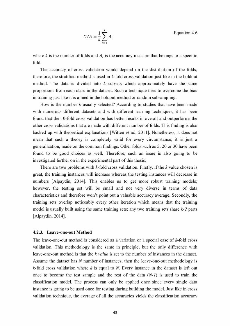
43
𝐶𝑉𝐴 =1
𝑘 𝐴𝑖
𝑘
𝑖=1
Equation 4.6
where k is the number of folds and 𝐴𝑖 is the accuracy measure that belongs to a specific
fold.
The accuracy of cross validation would depend on the distribution of the folds;
therefore, the stratified method is used in k-fold cross validation just like in the holdout
method. The data is divided into k subsets which approximately have the same
proportions from each class in the dataset. Such a technique tries to overcome the bias
in training just like it is aimed in the holdout method or random subsampling.
How is the number k usually selected? According to studies that have been made
with numerous different datasets and with different learning techniques, it has been
found that the 10-fold cross validation has better results in overall and outperforms the
other cross validations that are made with different number of folds. This finding is also
backed up with theoretical explanations [Witten et al., 2011]. Nonetheless, it does not
mean that such a theory is completely valid for every circumstance; it is just a
generalization, made on the common findings. Other folds such as 5, 20 or 30 have been
found to be good choices as well. Therefore, such an issue is also going to be
investigated further on in the experimental part of this thesis.
There are two problems with k-fold cross validation. Firstly, if the k value chosen is
great, the training instances will increase whereas the testing instances will decrease in
numbers [Alpaydin, 2014]. This enables us to get more robust training models;
however, the testing set will be small and not very diverse in terms of data
characteristics and therefore won’t point out a valuable accuracy average. Secondly, the
training sets overlap noticeably every other iteration which means that the training
model is usually built using the same training sets; any two training sets share k-2 parts
[Alpaydin, 2014].
4.2.3. Leave-one-out Method
The leave-one-out method is considered as a variation or a special case of k-fold cross
validation. This methodology is the same in principle, but the only difference with
leave-one-out method is that the k value is set to the number of instances in the dataset.
Assume the dataset has N number of instances, then the leave-one-out methodology is
k-fold cross validation where k is equal to N. Every instance in the dataset is left out
once to become the test sample and the rest of the data (N-1) is used to train the
classification model. The process can only be applied once since every single data
instance is going to be used once for testing during building the model. Just like in cross
validation technique, the average of all the accuracies yields the classification accuracy
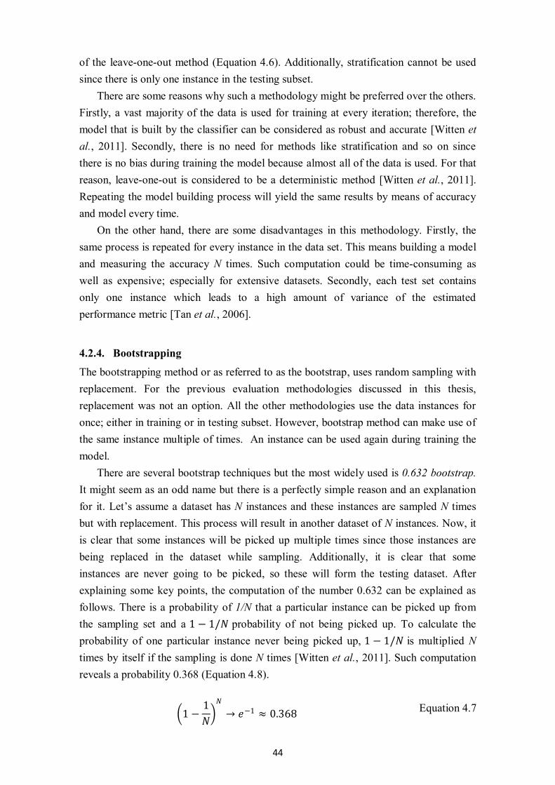
44
of the leave-one-out method (Equation 4.6). Additionally, stratification cannot be used
since there is only one instance in the testing subset.
There are some reasons why such a methodology might be preferred over the others.
Firstly, a vast majority of the data is used for training at every iteration; therefore, the
model that is built by the classifier can be considered as robust and accurate [Witten et
al., 2011]. Secondly, there is no need for methods like stratification and so on since
there is no bias during training the model because almost all of the data is used. For that
reason, leave-one-out is considered to be a deterministic method [Witten et al., 2011].
Repeating the model building process will yield the same results by means of accuracy
and model every time.
On the other hand, there are some disadvantages in this methodology. Firstly, the
same process is repeated for every instance in the data set. This means building a model
and measuring the accuracy N times. Such computation could be time-consuming as
well as expensive; especially for extensive datasets. Secondly, each test set contains
only one instance which leads to a high amount of variance of the estimated
performance metric [Tan et al., 2006].
4.2.4. Bootstrapping
The bootstrapping method or as referred to as the bootstrap, uses random sampling with
replacement. For the previous evaluation methodologies discussed in this thesis,
replacement was not an option. All the other methodologies use the data instances for
once; either in training or in testing subset. However, bootstrap method can make use of
the same instance multiple of times. An instance can be used again during training the
model.
There are several bootstrap techniques but the most widely used is 0.632 bootstrap.
It might seem as an odd name but there is a perfectly simple reason and an explanation
for it. Let’s assume a dataset has N instances and these instances are sampled N times
but with replacement. This process will result in another dataset of N instances. Now, it
is clear that some instances will be picked up multiple times since those instances are
being replaced in the dataset while sampling. Additionally, it is clear that some
instances are never going to be picked, so these will form the testing dataset. After
explaining some key points, the computation of the number 0.632 can be explained as
follows. There is a probability of 1/N that a particular instance can be picked up from
the sampling set and a 1 − 1/𝑁 probability of not being picked up. To calculate the
probability of one particular instance never being picked up, 1 − 1/𝑁 is multiplied N
times by itself if the sampling is done N times [Witten et al., 2011]. Such computation
reveals a probability 0.368 (Equation 4.8).
1 −1
𝑁 𝑁
→ 𝑒−1 ≈ 0.368
Equation 4.7

45
Now, if this computation is applied to a large dataset, it means that 36.8% of the
instances will probably never be picked up and will be used in testing subset. However,
the remaining 63.2% will probably be used at least once in training the model multiple
times. Thus, total of N instances will be used in building the model from training set.
This is the main explanation behind the 0.632 bootstrap method.
Bootstrapping method can be repeated as many times as it is necessary; there are not
any limitations like in leave-one out method. The final accuracy of bootstrap method is
calculated after all the repetitions are complete. After k times of repetition of bootstrap,
accuracy is calculated as summation of accuracies which are distributed in testing and
training subsets. The equation for the model, M, built by using bootstrap is below [Han
et al., 2011].
𝐴 𝑀 =1
𝑘 0.632 𝑥 𝐴(𝑀𝑖)𝑡𝑒𝑠𝑡𝑖𝑛 𝑔𝑠𝑒𝑡
𝑘
𝑖=1
+ 0.368 𝑥 𝐴(𝑀𝑖)𝑡𝑟𝑎𝑖𝑛𝑖𝑛𝑔 _𝑠𝑒𝑡
Equation 4.8
As mentioned earlier, the process can be repeated k many times and at each process,
63.2% form the training and 36.8% form the testing set. Combined accuracy of the
model that is generated at each iteration is calculated and then an average of all the
model accuracies is calculated that gives the overall accuracy of the model.

46
5. Research Method
Two different research methodologies have been used in this thesis. Literature review
has been the first methodology in the sense that the background information on decision
trees has been formed solidly. Then, literature was searched so that any information that
could be related with decision tree accuracy and its evaluation methods were understood
comprehensibly. These sorts of literature were also used to guide and manage the
experimental process in order to understand and interpret the results in a more
comprehensible fashion.
The second research methodology used is the experimental research strategy. In the
experimental part, tests were implemented in order to find patterns and understand the
relationship within decision tree accuracies that were evaluated by various different
evaluation methods.
In this part, the research methodologies that have been followed are going to be
discussed and explained in detail. The motivation behind these research methodologies,
validity of the methods, tools and techniques used in such methodologies are also stated.
Additionally, the data that has been used in the experiment is explained as well.
5.1. Motivation and Purpose of the Experiment
Decision trees are one of the most widely used machine learning algorithms as stated
earlier in the thesis. Decision trees create solutions to classification problems on various
different fields such as engineering, science, medical fields, and economical analytics.
For this reason, decision trees are considered to be one of the most powerful tools that
can accomplish such tasks [Kantardzic, 2011]. The possibility of being able to apply
decision trees in almost any classification and prediction field of data mining makes
decision trees essential. Therefore, accuracy of decision trees plays a key role especially
when there is more than one algorithm and evaluation model to choose from. Each
algorithm has its own methodology of building a model and the evaluation models also
play a big role in the process of building that specific model. The portions of the data to
be used are decided when building the decision tree model according to the choice of
the evaluation method. For example, when 50% holdout split is chosen, the model is
built using half of the available data. Another example would be when using the 10-fold
cross validation, the data is split into 10 partitions and a model is built using 9 partitions
and tested on the remaining one where this process is repeated 10 times. All these
choices of evaluation methods might have a great impact on the resulting accuracy and
decision tree model that is built accordingly with the evaluation method. Thus, finding
the correct evaluation method that would help build a better model and predict the
accuracy of the decision tree inducer is very important since it is the accuracy in the end
of an analysis that matters the most and that will lead to a good prediction in overall.
47
Although decision trees are widely and frequently applied in data mining and
machine learning context, there are not many studies that have made comparisons of
different decision tree algorithms regarding their performance when evaluated by
different methods. There are just some logical assumptions on which evaluation method
would perform better than the other according to some characteristics of the datasets
such the dataset size or number of attributes. Nonetheless, there is not a notion that has
been proven.
As a result, the aim of this thesis is to study how using different evaluation methods
might have effect on decision tree accuracies when they are applied to different decision
tree algorithms. Thus, five different decision tree algorithms were tested using five
different evaluation methods on ten different datasets. The results were analyzed
according to the accuracy measure and its standard deviation and standard error of
misclassification rate as evaluation measures.
5.2. Datasets
Choosing the datasets is essential in the experiment because the data that is chosen
needs to be reliable and applicable. Applicable means the data needs to be in the correct
format and ready for classification purposes. Additionally, not all types of data are
suitable for decision tree learning or classification to be specific. Therefore, the datasets
need to be chosen carefully and then should be preprocessed if it is not already.
For the experimental part of the thesis, all the datasets have been acquired from the
UCI machine learning repository [Bache and Lichman, 2015]. It is a very reliable
source of data where almost all the datasets are preprocessed or at least they are in
tabular format. This repository is mostly used for academic purposes because of the fact
that it is a reliable source of data. Hence, it is possible to confirm the validity and the
credibility of the all datasets that were used in the experiment.
Approximately twenty datasets were examined before the experiment; however,
only ten datasets were chosen due to some criteria. The chosen datasets are related with
various different fields including medical areas. Table 5.1 summarizes the details of the
datasets that are chosen according to numerous fields including; total number of
instances (cases), total number of classes, total number of attributes, missing values and
if the dataset is uniformly distributed or not.

48
Dataset No.
cases
No.
classes
No.
attributes
Continuous Categorical Missing
values
Uniform
distribution
Arrhythmia 452 16 279 207 72 Yes No
Audiology 226 24 69 0 69 Yes No Balance Scale 625 3 4 4 0 None No
Breast Cancer 286 2 9 0 9 Yes No
Glass 214 7 9 9 0 None No
Hepatitis 155 2 19 6 13 Yes No Ionosphere 351 2 34 34 0 None No
Iris 150 3 4 4 0 None Yes
Musk1 476 2 167 166 1 None Appx Zoo 101 6 18 1 17 None No
Table 5.1. Dataset summary.
All the necessary information is already given in the table but it would be beneficial
to explain the datasets and their context in more detail. For this reason, the datasets are
explained based on their context in the following part.
5.2.1. Detailed Dataset Explanations
Arrhythmia
Arrhythmia dataset is donated to the UCI repository in 1998 by Altay Guvenir from
Bilkent University. The data consists of 452 instances and 16 classes in total. There are
279 attributes in which are either continuous (207) or categorical (72). The dataset
contains some missing values and the classes of the data are not distributed uniformly.
The aim is to separate the different type of cardiac arrhythmia cases and to classify them
into one of 16 groups or classes in this case in order to distinguish the cases which have
arrhythmia or not. All the information regarding the attributes and classes cannot be
explained in detail in this thesis since there are a lot of different attributes and classes
involved in the dataset; however, those specific information could be accessed from the
repository [Guvenir et al., 1998].
Audiology
Standardized version of the audiology dataset is donated to the UCI repository in 1992
by Ross Quinlan but the primary donor was Professor Jergen from the Baylor College
of Medicine. The data consists of 226 instances and 24 classes in total. There are 69
attributes which all of them are categorical. The dataset contains some missing values
and the classes of the data are not distributed uniformly. The aim is to separate the
different type of audiology disorder causes and to classify them into one of 24 groups or
classes in order to distinguish the cases according to audiological disorder causes. All
the information regarding the attributes and classes cannot be explained in detail, but
those specific information could be accessed from the repository [Jergen, 1992].

49
Balance Scale
The dataset is donated to UCI repository in 1994 by Tim Hume from Carnegie-Mellon
University. It is an interesting and extraordinary dataset. The dataset has 625 instances,
3 classes and 4 attributes which are all continuous. It does not have any missing values
and the classes are not distributed uniformly. The best explanation and the aim of the
dataset is given by Hume himself; “This data set was generated to model psychological
experimental results. Each example is classified as having the balance scale tip to the
right, tip to the left, or be balanced. The attributes are the left weight, the left distance,
the right weight, and the right distance. The correct way to find the class is the greater
of (left-distance * left-weight) and (right-distance * right-weight). If they are equal, it is
balanced [Hume, 1994].”
Breast Cancer
Breast cancer dataset is donated to UCI repository in 1988 by Ming Tan and Jeff
Schlimmer who work in Carnegie-Mellon University. However, the original source of
the data is Matjaz Zwitter and Milan Soklic who are physicians in the oncology
department of University Medical center in Ljubljana, former Yugoslavia. The dataset
has 286 instances, 2 classes and 9 attributes which all of them are categorical. It only
has 8 missing attribute values in the dataset and the class values are not distributed
uniformly. The aim of the dataset is to try and find out if breast cancer will occur again
or not; therefore, all the attributes are related with breast cancer. For instance the
attributes include; age, menopause, tumor size, inv-nodes (the number of auxiliary
lymph nodes that contain metastatic breast cancer visible in histological examination),
node caps, degree of malignancy, breast (left, right), breast quadrant and irradiation.
More detailed information about the dataset can be accessed in the repository [Zwitter
and Soklic, 1988].
Glass Identification
Glass identification dataset is also another interesting dataset which was donated by
Vina Spiehler but the original owner of the data is B. German from Central Research
Establishment Reading, England. The dataset has 214 instances, 7 classes and 9
attributes which all of them are continuous. It does not have any missing values and its
class values are not distributed uniformly. The aim of the dataset is to classify glasses
into seven certain types of groups with the help of nine chemical elements. Therefore,
the attributes used to classify the glasses are; refractive index, sodium (Na), magnesium
(Mg), aluminum (Al), silicon (Si), potassium (K), calcium (Ca), barium (Ba) and iron
(Fe). The types of glasses that are trying to be classified are; building windows float
processed, building windows non float processed, vehicle windows float processed,
vehicle windows non float processed, containers, tableware and headlamps. More

50
detailed information on the dataset and other researches related to it can be found in the
repository [German, 1987].
Hepatitis
Hepatitis is also another important dataset that has been used in many researches. It
belongs to Gail Gong from Carnegie-Mellon University and has been donated in 1988.
The dataset has 155 instances, 19 attributes where 6 of them are continuous and 13 of
them are categorical. It has missing values and the attributes are not distributed
uniformly including the class attribute. The aim of the dataset is to classify hepatitis
cases according to previous patient mortality; the patient lived or died. All the
information regarding the attributes cannot be explained in detail in this thesis since
there are a lot of different attributes involved in the dataset; however, those specific
information could be accessed from the repository [Gong, 1988].
Ionosphere
Ionosphere dataset is donated to the UCI repository in 1989 by Vince Sigillito from
Space Physics Group. The data consists of 351 instances, 2 classes, 34 attributes and all
of the attributes are continuous. The dataset does not have any missing values and is
not distributed uniformly. The content and the aim of the data are best explained by
Sigillito himself “This radar data was collected by a system in Goose Bay, Labrador.
This system consists of a phased array of 16 high-frequency antennas with a total
transmitted power on the order of 6.4 kilowatts. The targets were free electrons in the
ionosphere. "Good" radar returns are those showing evidence of some type of structure
in the ionosphere. "Bad" returns are those that do not; their signals pass through the
ionosphere. Received signals were processed using an autocorrelation function whose
arguments are the time of a pulse and the pulse number. There were 17 pulse numbers
for the Goose Bay system. Instances in this database are described by 2 attributes per
pulse number, corresponding to the complex values returned by the function resulting
from the complex electromagnetic signal [Sigillito, 1989].”
Iris
Iris data is a very important dataset that has been used widely in the field of machine
learning and in some cases it is even used as an example dataset. It contains 150
instances, 3 classes, 4 attributes and all of the attributes are continuous. The data does
not have any missing values and is uniformly distributed. Iris dataset’s history dates
back to 1932 and it was collected to quantify the morphologic variation of Iris flowers
of the three related species; Iris-setosa, Iris-versicolor and Iris-virginica. The attributes
reveal information related to the plant’s morphological structure; sepal length, sepal
width, petal length and petal width. As understood from the dataset features, its aim is

51
to classify data instances into 3 different iris plant types. More detailed information
about the data itself can be found in the repository [Fisher, 1988].
Musk1
Musk1 data is donated to UCI repository by Tom Dietterich from Oregon State
University in 1994. The data contains 476 instances, 167 attributes where 166 are
continuous and 1 is categorical. There are no missing values in the dataset and the data
is approximately distributed uniformly. The aim and the content of the data is as follows
“This dataset describes a set of 92 molecules of which 47 are judged by human experts
to be musks and the remaining 45 molecules are judged to be non-musks. The goal is to
learn to predict whether new molecules will be musks or non-musks. However, the 166
features that describe these molecules depend upon the exact shape, or conformation, of
the molecule… When learning a classifier for this data, the classifier should classify a
molecule as "musk" if ANY of its conformations is classified as a musk. A molecule
should be classified as "non-musk" if NONE of its conformations is classified as a musk
[Dietterich, 1994].” More detailed information about the dataset can be found in the
repository.
Zoo
Zoo dataset is the smallest dataset that has been used in this thesis. The dataset belongs
to Richard Forsyth and is donated by him to the UCI repository in 1990. It consists of
101 instances, 6 classes, 18 attributes where 17 of them are categorical and 1 of them is
continuous. The dataset does not have any missing values and it is not distributed
uniformly. The aim of the data is to classify a wide range of animals into 7 classes by
the help of attributes that are related to animal characteristics such as: toothed, aquatic,
number of legs. All the information regarding the attributes cannot be explained in
detail in this thesis since there are a lot of different attributes involved in the dataset, but
those specific information could be accessed from the repository [Forsyth, 1990].
5.2.2. Preprocessing the Datasets
Some of the datasets that were chosen had to be preprocessed although their formats
were correct. The preprocessing that was applied to the datasets include discretization,
removing useless attributes with a lot of missing values and also changing the format of
missing values.
Firstly, all of the datasets were analyzed one by one to check if any attribute in the
datasets had any missing values and if they were relevant to the dataset or not. There
were four datasets that had missing attribute values, and these datasets had the highest
probability of having meaningless attributes. The reason behind this notion is simply
because of the amount of missing values might have great impact on the attributes and
make those attributes irrelevant to the datasets.

52
All of the datasets were examined and the datasets without missing values did not
require any preprocessing. However, the four datasets with missing values needed more
analysis so all the attributes that had the majority of their values missing were analyzed
one by one for each dataset. The attributes were dropped from the dataset and were
tested if they had any impact on predictive and descriptive accuracy using different
evaluation methods including the holdout 66 split, 10-fold cross validation and leave-
one-out method. The same splits were used in the tests and the data instances were
identical in each test (for attribute dropped version and the original versions). If were
any impact on the results, the attributes were kept and otherwise dropped.
The first dataset that had missing values was the Arrhythmia dataset. There were 5
attributes with missing values; T, P, QRST, J and heart rate where the amount of
missing values were 8, 22, 1, 376 and 1 respectively (Table 5.2). The only attribute that
had a major effect was J which had 83% of its values missing. If the attribute was taken
out there was a 5-10 percent change in accuracy, so it was decided not to remove the
attribute from the dataset. As a result, 98.21% of the attribute values in total were valid
and none of the attributes were removed.
Attributes Missing values (Amount) Missing values (Percentage)
T 8 1.8 %
P 22 4.85 %
QRST 1 0.2 %
J 376 83.2 %
Heart rate 1 0.2 %
Table 5.2. Arrhythmia missing values.
The second dataset that had missing values was the Audiology dataset (Table 5.3).
There were 7 attributes with missing values; ar_c, ar_u, bone, bser, o_ar_c, o_ar_u and
speech where the amount of missing values were 4(1.8%), 3(1.3%), 75(33.2%),
222(98%), 5(2.2%), 2(0.8%), 6(2.65%). Bser attribute had the majority of its values
missing so it was taken out and tested if anything by means of accuracy would change
and at each test the accuracy did not have any effect. Consequently, bser attribute was
removed from the dataset and after the removal dataset had 91.3% valid values.
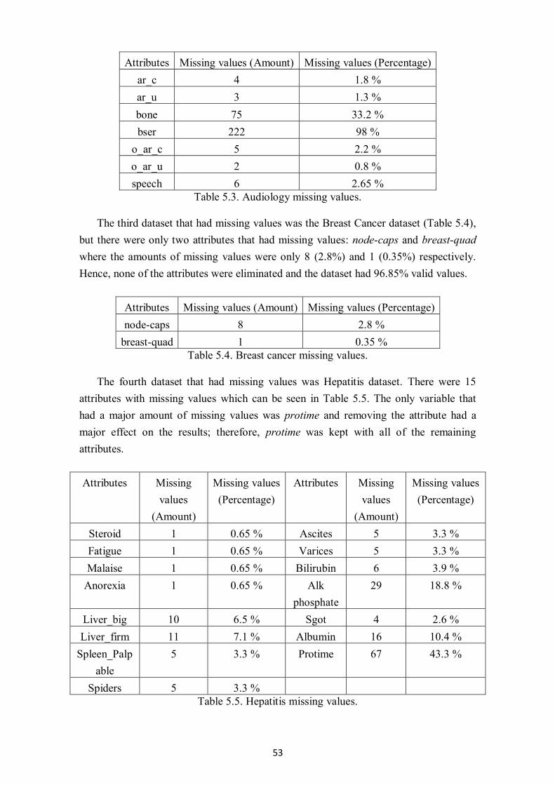
53
Attributes Missing values (Amount) Missing values (Percentage)
ar_c 4 1.8 %
ar_u 3 1.3 %
bone 75 33.2 %
bser 222 98 %
o_ar_c 5 2.2 %
o_ar_u 2 0.8 %
speech 6 2.65 %
Table 5.3. Audiology missing values.
The third dataset that had missing values was the Breast Cancer dataset (Table 5.4),
but there were only two attributes that had missing values: node-caps and breast-quad
where the amounts of missing values were only 8 (2.8%) and 1 (0.35%) respectively.
Hence, none of the attributes were eliminated and the dataset had 96.85% valid values.
Attributes Missing values (Amount) Missing values (Percentage)
node-caps 8 2.8 %
breast-quad 1 0.35 %
Table 5.4. Breast cancer missing values.
The fourth dataset that had missing values was Hepatitis dataset. There were 15
attributes with missing values which can be seen in Table 5.5. The only variable that
had a major amount of missing values was protime and removing the attribute had a
major effect on the results; therefore, protime was kept with all of the remaining
attributes.
Attributes Missing
values
(Amount)
Missing values
(Percentage)
Attributes Missing
values
(Amount)
Missing values
(Percentage)
Steroid 1 0.65 % Ascites 5 3.3 %
Fatigue 1 0.65 % Varices 5 3.3 %
Malaise 1 0.65 % Bilirubin 6 3.9 %
Anorexia 1 0.65 % Alk
phosphate
29 18.8 %
Liver_big 10 6.5 % Sgot 4 2.6 %
Liver_firm 11 7.1 % Albumin 16 10.4 %
Spleen_Palp
able
5 3.3 % Protime 67 43.3 %
Spiders 5 3.3 %
Table 5.5. Hepatitis missing values.
54
After the attributes with missing values were checked and the necessary removals
were made, the datasets were almost ready. All the algorithms except CHAID were
compatible with continuous attributes; therefore, the datasets that contained continuous
attributes needed to be discretized in order run tests on the RapidMiner tool. Hence,
discretization was applied to all of the datasets except Audiology and Breast Cancer.
The discretization was performed by the equal frequency binning and the thresholds of
the bins were selected so that all bins contain the same number of numerical values.
Equal frequency binning was chosen due to lack of choices provided by the RapidMiner
tool. Numerical values were assigned to the bin representing the range segment
covering the numerical values. In the discretization process, the number of bins varied
according to the characteristics of the data and its attribute values; the number of bins
which were chosen was either two or three. The ideal number of bins was determined
experimentally and the number of bins which performed optimal were chosen. In this
process, histograms were used to examine the data and different intervals were tried
accordingly. During the experimentation a wide range of bins were tested. The
discretized versions of the datasets were only used in the CHAID algorithm analysis and
for the rest of the algorithms the non-discretized versions of the datasets were used.
Lastly, RapidMiner and IBM SPSS Modeler did not recognize the missing values
automatically since “?” was used to represent missing values. Consequently, all of the
datasets’ missing values were replaced with null values instead of “?”, which is the
missing value format of WEKA and C5.0 tools. All of the datasets’ missing values were
adjusted accordingly before the tests that were made on RapidMiner and IBM SPSS
Modeler.
5.3. Algorithms and Evaluation Methods Chosen
There is a great range of different decision tree algorithms available but not all of them
are available in data mining tools and again not all of them are worth exploring. In this
thesis, four different decision tree algorithms were chosen according to their well
known performance in both private sectors and academic researches. Hence, the chosen
algorithms are the ones that have been discussed in the thesis; the well known C4.5,
C5.0, CART and CHAID. Additionally, boosting option of C5.0 has also been tested
since it would be interesting to compare the results with other algorithms in such
context. Consequently, there were five different algorithms including the boosted C5.0
algorithm.
The most widely used evaluation methods have been chosen to assess the selected
five decision tree algorithms. These evaluation methods include leave-one-out method,
5-fold cross validation, 10-fold cross validation, holdout method with 50 percent split
ratio and holdout method with 66 percent split ratio.

55
5.4. Tools Used
In order to accomplish good academic research and experiments on decision trees, tools
are vital. Choosing the correct tools for the job plays an important part in the academic
research and also in private businesses as well. Not all the tools have all the machine
learning and data mining algorithms built in; therefore, tools were chosen based on the
methods and algorithms that were going to be employed. In this case, four decision tree
algorithms were chosen to be tested on various evaluation methods; C4.5, C5.0, CART
and CHAID. These were chosen since they are the most widely used decision tree
algorithms in business and academic areas.
After the selection of algorithms were made, tools had to be selected based on
which algorithms were implemented in which tools. In the end, CART and C4.5 were
correctly implemented in the tool WEKA, CHAID was implemented in IBM SPSS
Modeler and C5.0 had its own tool which could be used under GNU license as
noncommercial purposes.
5.4.1. WEKA
Waikato Environment for Knowledge Analysis (WEKA) is a tool specifically made for
machine learning purposes by the University of Waikato. It is a collection of machine
learning algorithms and data preprocessing tools for researchers and practitioners of
machine learning and data mining [Hall et al., 2009]. The collection includes algorithms
for classification, regression, clustering and association rule mining. Additionally,
graphical user interfaces and visualization options can be used for data exploration and
algorithm evaluation. Data preprocessing is also another capability where different file
formats are supported such as ARFF (which is the native file format of WEKA), CSV,
Matlab ASCII files and so on [Bouckaert et al., 2010]. The current version of WEKA is
implemented by using JAVA programming language; therefore, it can run on any
machine and operating system. It is a very easy to use and efficient program.
The reason why WEKA is chosen for the experiments is that the decision tree
algorithms CART and especially C4.5 are almost identically implemented when
compared with the original algorithms. These implementations exist under the
classification and regression capabilities of the tool.
5.4.2. IBM SPSS Modeler
IBM Statistical Package for the Social Sciences Modeler (SPSS Modeler) is a data
mining and text analytics based tool that has been implemented by SPSS Inc. for
predictive and analytical analysis purposes. The company SPSS Inc. has been acquired
by IBM in 2009.
It provides various complex and advanced data mining algorithms, methods and
techniques. These algorithms, methods and techniques are applied as models, so one can

56
build models for many different analysis purposes. Such an option makes the process
visual and easily understandable for the majority of users. It also fastens the analysis
process due to simpler user experience. The tool is widely used in different industrial
fields such as customer analytics and customer relationship management (CRM), fraud
detection and prevention, forecasting demands and sales, healthcare quality
improvement, academic researches, telecommunications and many other [IBM, 2014a].
The tool provides algorithms from machine learning and data mining. Some of the
algorithms included are: decision trees, support vector machines, naïve bayes,
generalized linear mixed model, K-nearest neighbor algorithm and so on [IBM, 2014b].
The main reason IBM SPSS Modeler was chosen in this thesis is because it contains
implementations of the CHAID and C5.0 algorithms. Other decision tree
implementation in SPSS are; Exhaustive CHAID, CART and QUEST.
5.4.3. C5.0/See5
As discussed earlier in the thesis, C5.0 is an algorithm that has followed the earlier C4.5
decision tree algorithm. The computer program See5 is also implemented by Ross
Quinlan [Quinlan, 2004]. It has two versions; one is a single threaded version which is
open source and under GNU General Public License. It has dataset size limitations and
can be used for academicals purposes easily. The other version is the multithreaded
version which is commercially used in some products such as the IBM SPSS Modeller.
Besides being used commercially, it is also integrated into some open source
applications. For instance, another important statistical analysis tool R has a separate
package that utilizes the open source C5.0 algorithm implementation.
See5 can produce rulesets and decision trees. Additionally, it has a boosting option
built in which enables the algorithm to give better results under extensive datasets. This
tool is chosen because it gives a very simple and easy to use implementation of C5.0.
5.4.4. RapidMiner
RapidMiner is also another important and widely used tool that has a similar approach
as the IBM SPSS Modeler. The tool also uses models to build the process which again
makes the process visual, easily understandable and fastens the process of building an
analytical model and applying it. It provides an environment for machine learning, data
mining, text mining, predictive analytics and business analytics. It is used in business
and industrial applications and for academic researches. The tool provides usage for
research, education, training, rapid prototyping, application development and all steps
of data mining from visualization to validation and optimization [Hofmann and
Klinkenberg, 2013].

57
The tool is chosen since it provides many algorithms in data mining and machine
learning including decision trees such as CHAID, exhaustive CHAID and also provides
all the types of evaluation methods with the algorithms.
5.4.5. Other Tools
During the experimental part, 8-10 different data mining tools were analyzed and tested
in order to find the ones that are going to work with all the evaluation methods and also
would give stable and trustable results. Besides the tools explained above which have
been used in the experiments, there have also been some other tools that would have
been chosen if they had all possible evaluation methods that could be applied to the
algorithms. Some of the notable tools are R, StatSoft Statistica, Orange, IBM SPSS
Statistics and similar tools.
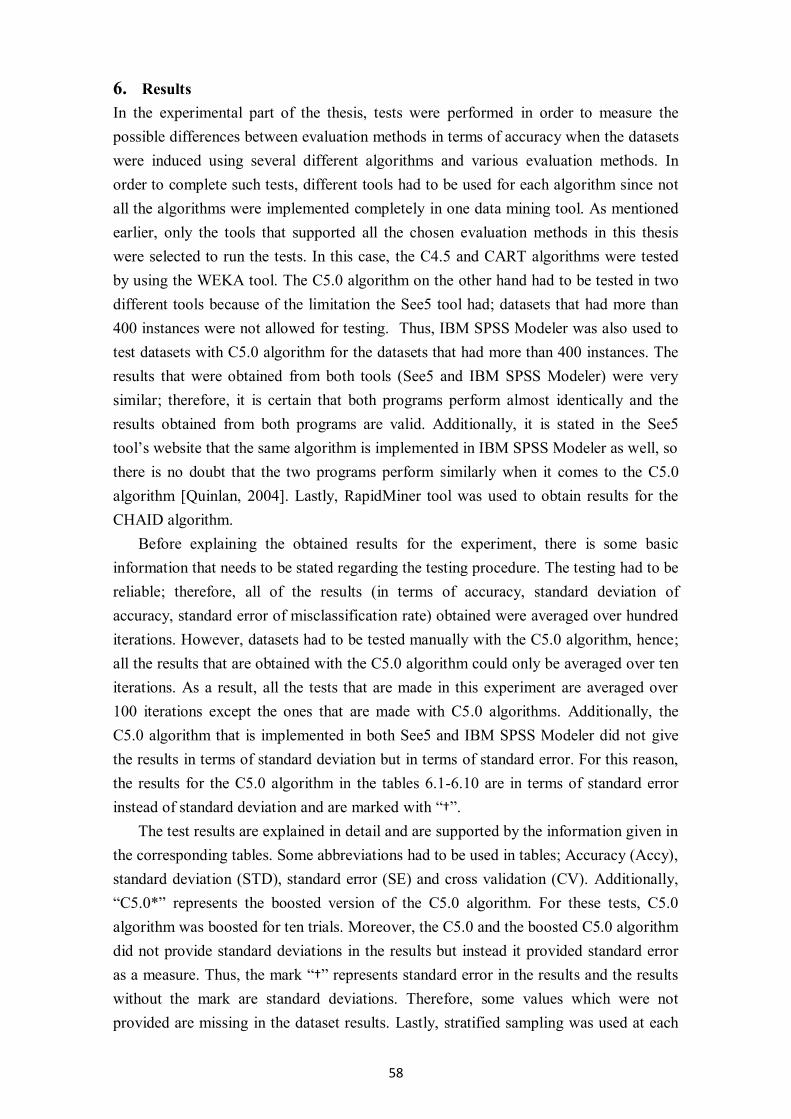
58
6. Results
In the experimental part of the thesis, tests were performed in order to measure the
possible differences between evaluation methods in terms of accuracy when the datasets
were induced using several different algorithms and various evaluation methods. In
order to complete such tests, different tools had to be used for each algorithm since not
all the algorithms were implemented completely in one data mining tool. As mentioned
earlier, only the tools that supported all the chosen evaluation methods in this thesis
were selected to run the tests. In this case, the C4.5 and CART algorithms were tested
by using the WEKA tool. The C5.0 algorithm on the other hand had to be tested in two
different tools because of the limitation the See5 tool had; datasets that had more than
400 instances were not allowed for testing. Thus, IBM SPSS Modeler was also used to
test datasets with C5.0 algorithm for the datasets that had more than 400 instances. The
results that were obtained from both tools (See5 and IBM SPSS Modeler) were very
similar; therefore, it is certain that both programs perform almost identically and the
results obtained from both programs are valid. Additionally, it is stated in the See5
tool’s website that the same algorithm is implemented in IBM SPSS Modeler as well, so
there is no doubt that the two programs perform similarly when it comes to the C5.0
algorithm [Quinlan, 2004]. Lastly, RapidMiner tool was used to obtain results for the
CHAID algorithm.
Before explaining the obtained results for the experiment, there is some basic
information that needs to be stated regarding the testing procedure. The testing had to be
reliable; therefore, all of the results (in terms of accuracy, standard deviation of
accuracy, standard error of misclassification rate) obtained were averaged over hundred
iterations. However, datasets had to be tested manually with the C5.0 algorithm, hence;
all the results that are obtained with the C5.0 algorithm could only be averaged over ten
iterations. As a result, all the tests that are made in this experiment are averaged over
100 iterations except the ones that are made with C5.0 algorithms. Additionally, the
C5.0 algorithm that is implemented in both See5 and IBM SPSS Modeler did not give
the results in terms of standard deviation but in terms of standard error. For this reason,
the results for the C5.0 algorithm in the tables 6.1-6.10 are in terms of standard error
instead of standard deviation and are marked with “†”.
The test results are explained in detail and are supported by the information given in
the corresponding tables. Some abbreviations had to be used in tables; Accuracy (Accy),
standard deviation (STD), standard error (SE) and cross validation (CV). Additionally,
“C5.0*” represents the boosted version of the C5.0 algorithm. For these tests, C5.0
algorithm was boosted for ten trials. Moreover, the C5.0 and the boosted C5.0 algorithm
did not provide standard deviations in the results but instead it provided standard error
as a measure. Thus, the mark “†” represents standard error in the results and the results
without the mark are standard deviations. Therefore, some values which were not
provided are missing in the dataset results. Lastly, stratified sampling was used at each

59
test so that there was a balance between the distribution of the chosen instances in both
training and testing data. The best result for each algorithm in the dataset results was
written in bold face for each of the following tables.
Arrhythmia Leave-one-out 5-Fold CV 10-Fold CV Holdout 50/50 Holdout 66/34
Accy. STD|SE Accy. STD|SE Accy. STD|SE Accy. STD|SE Accy. STD|SE
C4.5 66.37 - 65.74 3.98 65.83 5.86 64.57 3.18 65.53 3.19 CART 73.23 - 70.49 3.84 71.40 5.44 67.22 2.97 69.05 3.15 C5.0 69.00 2.20† 66.74 1.79† 67.42 1.97† 65.30 - 67.07 - C5.0 * 71.90 2.10† 72.00 1.91† 72.16 1.48† 71.28 - 71.31 - CHAID 53.10 - 48.47 6.24 54.09 1.82 51.68 14.76 45.19 17.09
Table 6.1. Arrhythmia test results.
Arrhythmia dataset was tested and the results are displayed in Table 6.1. According
to the results, leave-one-out method has been the best evaluation method for this dataset
since three out of five highest measured accuracies of the algorithms belong to the
leave-one-out method. In most of the cases, there is a 0.5-2 percent difference in terms
of accuracy when compared with the second best method which is 10-Fold CV. 5-Fold
CV is the third best after 10-Fold CV; however, there is a slight difference between both
so it could be counted as a draw between them. The fourth best is Holdout 66 split
followed by the Holdout 50 split which is the poorest in terms of accuracy. Again there
is not much difference between the two holdout splits. The most unexpected
performance belonged to the CHAID algorithm since it had very poor results when
compared with other algorithms. Lastly, the best algorithm overall was the boosted C5.0
in terms of accuracy.
Audiology Leave-one-out 5-Fold CV 10-Fold CV Holdout 50/50 Holdout 66/34
Accy. STD|SE Accy. STD|SE Accy. STD|SE Accy. STD|SE Accy. STD|SE
C4.5 77.88 - 77.38 4.55 77.35 7.39 75.55 3.43 77.40 3.30 CART 75.66 - 74.34 5.43 74.93 7.83 69.60 4.03 73.20 4.74 C5.0 77.90 2.80† 77.69 1.87† 77.52 2.42† 71.51 - 74.21 - C5.0 * 84.10 2.40† 84.16 2.06† 84.70 2.04† 77.79 - 79.72 - CHAID 30.53 - 37.28 4.79 37.17 1.63 47.26 13.92 45.36 15.62
Table 6.2. Audiology test results.
The results in Table 6.2 belong to the Audiology dataset. Leave-one-out is the best
evaluation method in terms of accuracy when compared with the other methods but the
difference between the accuracies are very small. The second best is 5-Fold CV but
again the accuracy difference between 10-Fold CV which is the third best, is very small
so that both methodologies basically performed identically. Then the Holdout 66 split is
the fourth best followed by the Holdout 50 split. Holdout 66 split is visibly better than
Holdout 50 in all of the algorithms except CHAID which performed very poorly and
way unstable since the STDs of the holdout methods were very high when compared
with other algorithms’ STDs. Additionally, the algorithm that performed best is boosted

60
C5.0 in most cases with 2-6 percent difference in terms of accuracy when compared
with other algorithms.
Balance Scale Leave-one-out 5-Fold CV 10-Fold CV Holdout 50/50 Holdout 66/34
Accy. STD|SE Accy. STD|SE Accy. STD|SE Accy. STD|SE Accy. STD|SE
C4.5 77.76 - 78.27 2.96 77.93 4.09 78.08 1.88 78.28 2.22 CART 79.36 - 78.46 2.93 79.15 4.09 77.88 1.80 78.52 2.00 C5.0 77.80 1.70† 78.66 1.12† 77.85 1.30† 77.49 - 78.79 - C5.0 * 81.10 1.60† 83.47 1.15† 82.74 1.09† 83.58 - 84.52 - CHAID 74.56 - 76.93 0.79 76.48 0.52 74.87 2.27 76.44 2.40
Table 6.3. Balance scale test results.
Holdout 66 split was the best evaluation method for the Balance Scale dataset
according to the results in Table 6.3. However, 5-Fold CV has performed almost
identically to Holdout 66 split with only 0-0.5 percent differences when compared. 10-
Fold CV was the third best evaluation method after the 5-Fold CV. The two worst
methods are Holdout 50 split and leave-one-out method. The dataset results could be
considered stable since the standard deviations are low even when compared with other
dataset results in general. The best algorithm in terms of accuracy is the boosted C5.0
for this dataset as well.
Breast Cancer Leave-one-out 5-Fold CV 10-Fold CV Holdout 50/50 Holdout 66/34
Accy. STD|SE Accy. STD|SE Accy. STD|SE Accy. STD|SE Accy. STD|SE
C4.5 75.52 - 72.77 4.09 73.93 5.65 71.19 2.62 71.37 3.51 CART 72.03 - 70.01 3.85 70.71 5.34 69.55 2.73 69.95 2.84 C5.0 75.50 2.50† 71.71 1.82† 73.30 2.12† 73.95 - 69.36 - C5.0 * 75.50 2.50† 71.18 2.11† 73.84 2.00† 71.58 - 70.81 - CHAID 64.49 - 64.36 2.29 64.33 1.87 64.53 3.78 64.82 4.96
Table 6.4. Breast cancer test results.
Breast cancer results are given in Table 6.4 and according to those results, leave-
one-out is the best evaluation method for the dataset. It gave 1.5-2 percent better
performance in terms of accuracy when compared with the second best method which is
the 10-Fold CV. Then it is 5-Fold CV which is the third best by the accuracy measure.
Lastly, both holdout methods have very close results; however, it could be stated that
Holdout 66 is better since it performed slightly better than Holdout 50 except for the
C5.0 algorithms. Furthermore, C5.0 and the boosted C5.0 algorithm performed almost
identically in every evaluation method. Additionally, the dataset has relatively stable
results when compared with other datasets since the STDs do not vary much. For this
dataset, C4.5 performed slightly better than other algorithms in general. This is
interesting since the boosted C5.0 had been performing very well on the other datasets.

61
Glass Leave-one-out 5-Fold CV 10-Fold CV Holdout 50/50 Holdout 66/34
Accy. STD|SE Accy. STD|SE Accy. STD|SE Accy. STD|SE Accy. STD|SE
C4.5 66.82 - 67.30 6.38 67.88 9.12 65.56 4.08 66.69 5.08 CART 72.90 - 70.24 6.16 70.49 8.48 65.33 4.88 68.55 5.57 C5.0 65.90 3.20† 69.00 3.29† 70.36 2.95† 66.60 - 65.27 - C5.0 * 76.20 2.90† 73.69 2.61† 77.06 2.55† 70.28 - 73.29 - CHAID 62.62 - 61.68 2.10 62.60 1.65 57.85 4.89 60.71 4.93
Table 6.5. Glass test results.
Table 6.5 shows the results for the Glass dataset. It could be argued from the results
that 10-Fold CV is the best method when compared with the rest. Then, leave-one-out
method is the second best followed by the 5-Fold CV. The worst methods are again the
holdout splits in terms of accuracy. However, Holdout 66 is better in most cases with
0.5-3.00 percent better accuracies. The dataset is slightly unstable since the STDs of the
holdout methods reach higher intervals; 4-5 percent. The best algorithm overall is again
the boosted C5.0 with clear differences in terms of accuracy.
Hepatitis Leave-one-out 5-Fold CV 10-Fold CV Holdout 50/50 Holdout 66/34
Accy. STD|SE Accy. STD|SE Accy. STD|SE Accy. STD|SE Accy. STD|SE
C4.5 80.00 - 79.03 5.81 79.26 8.72 78.81 3.86 78.68 4.69 CART 71.61 - 78.82 4.75 77.48 6.82 79.49 2.84 79.32 3.34 C5.0 78.70 3.30† 79.62 2.78† 78.75 2.83† 81.57 - 79.05 - C5.0 * 83.20 3.00† 83.35 3.03† 84.42 2.62† 80.89 - 81.69 - CHAID 79.35 - 78.80 2.34 80.21 2.32 77.99 3.88 78.32 4.70
Table 6.6. Hepatitis test results.
The results in Table 6.6 show the results for the Hepatitis dataset. Firstly, all the
results in the dataset are very close to each other apart from some exceptions. If one had
to decide the best evaluation method for this dataset, it would be 10-Fold cross
validation although it is tied up with Holdout 50 split. However, when the Holdout 50 is
compared with the 10-Fold CV, 10-Fold CV is slightly better. Strangely, when each
algorithm is compared one by one, 5-Fold is second best followed by the leave-one-out
method. Once again the two worst methods are considered to be the holdout splits.
Nevertheless, it should be stated that it is not a very reliable dataset since it has a
significant amount of missing values and the STDs are relatively higher. Additionally,
there is one more fact that has not changed once again; the algorithm that performed
best overall is the boosted C5.0.
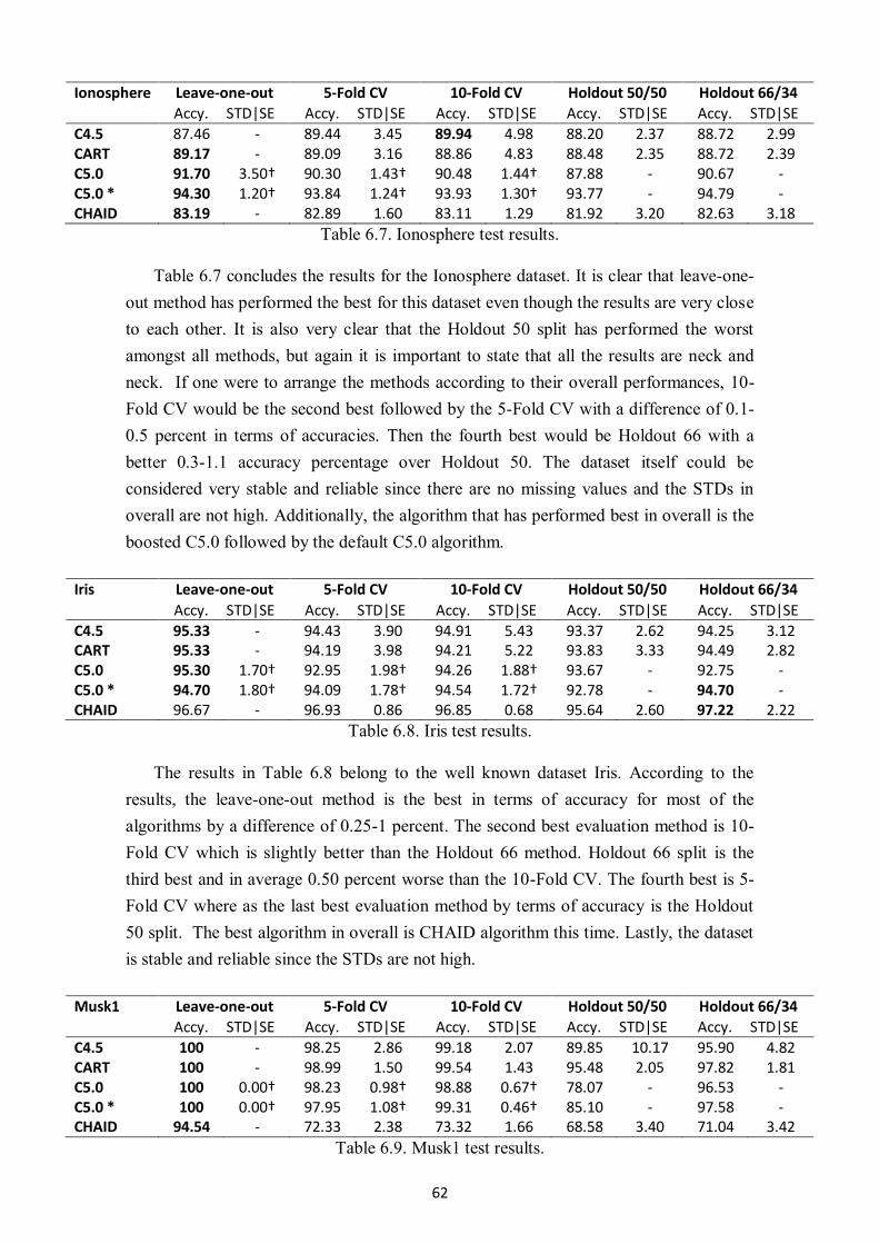
62
Ionosphere Leave-one-out 5-Fold CV 10-Fold CV Holdout 50/50 Holdout 66/34
Accy. STD|SE Accy. STD|SE Accy. STD|SE Accy. STD|SE Accy. STD|SE
C4.5 87.46 - 89.44 3.45 89.94 4.98 88.20 2.37 88.72 2.99 CART 89.17 - 89.09 3.16 88.86 4.83 88.48 2.35 88.72 2.39 C5.0 91.70 3.50† 90.30 1.43† 90.48 1.44† 87.88 - 90.67 - C5.0 * 94.30 1.20† 93.84 1.24† 93.93 1.30† 93.77 - 94.79 - CHAID 83.19 - 82.89 1.60 83.11 1.29 81.92 3.20 82.63 3.18
Table 6.7. Ionosphere test results.
Table 6.7 concludes the results for the Ionosphere dataset. It is clear that leave-one-
out method has performed the best for this dataset even though the results are very close
to each other. It is also very clear that the Holdout 50 split has performed the worst
amongst all methods, but again it is important to state that all the results are neck and
neck. If one were to arrange the methods according to their overall performances, 10-
Fold CV would be the second best followed by the 5-Fold CV with a difference of 0.1-
0.5 percent in terms of accuracies. Then the fourth best would be Holdout 66 with a
better 0.3-1.1 accuracy percentage over Holdout 50. The dataset itself could be
considered very stable and reliable since there are no missing values and the STDs in
overall are not high. Additionally, the algorithm that has performed best in overall is the
boosted C5.0 followed by the default C5.0 algorithm.
Iris Leave-one-out 5-Fold CV 10-Fold CV Holdout 50/50 Holdout 66/34
Accy. STD|SE Accy. STD|SE Accy. STD|SE Accy. STD|SE Accy. STD|SE
C4.5 95.33 - 94.43 3.90 94.91 5.43 93.37 2.62 94.25 3.12 CART 95.33 - 94.19 3.98 94.21 5.22 93.83 3.33 94.49 2.82 C5.0 95.30 1.70† 92.95 1.98† 94.26 1.88† 93.67 - 92.75 - C5.0 * 94.70 1.80† 94.09 1.78† 94.54 1.72† 92.78 - 94.70 - CHAID 96.67 - 96.93 0.86 96.85 0.68 95.64 2.60 97.22 2.22
Table 6.8. Iris test results.
The results in Table 6.8 belong to the well known dataset Iris. According to the
results, the leave-one-out method is the best in terms of accuracy for most of the
algorithms by a difference of 0.25-1 percent. The second best evaluation method is 10-
Fold CV which is slightly better than the Holdout 66 method. Holdout 66 split is the
third best and in average 0.50 percent worse than the 10-Fold CV. The fourth best is 5-
Fold CV where as the last best evaluation method by terms of accuracy is the Holdout
50 split. The best algorithm in overall is CHAID algorithm this time. Lastly, the dataset
is stable and reliable since the STDs are not high.
Musk1 Leave-one-out 5-Fold CV 10-Fold CV Holdout 50/50 Holdout 66/34
Accy. STD|SE Accy. STD|SE Accy. STD|SE Accy. STD|SE Accy. STD|SE
C4.5 100 - 98.25 2.86 99.18 2.07 89.85 10.17 95.90 4.82 CART 100 - 98.99 1.50 99.54 1.43 95.48 2.05 97.82 1.81 C5.0 100 0.00† 98.23 0.98† 98.88 0.67† 78.07 - 96.53 - C5.0 * 100 0.00† 97.95 1.08† 99.31 0.46† 85.10 - 97.58 - CHAID 94.54 - 72.33 2.38 73.32 1.66 68.58 3.40 71.04 3.42
Table 6.9. Musk1 test results.
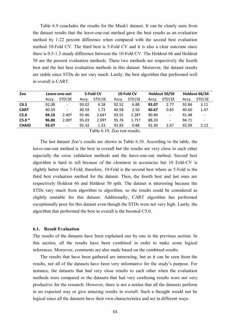
63
Table 6.9 concludes the results for the Musk1 dataset. It can be clearly seen from
the dataset results that the leave-one-out method gave the best results as an evaluation
method by 1-22 percent difference when compared with the second best evaluation
method 10-Fold CV. The third best is 5-Fold CV and it is also a clear outcome since
there is 0.5-1.3 steady difference between the 10-Fold CV. The Holdout 66 and Holdout
50 are the poorest evaluation methods. These two methods are respectively the fourth
best and the last best evaluation methods in this dataset. Moreover, the dataset results
are stable since STDs do not vary much. Lastly, the best algorithm that performed well
in overall is CART.
Zoo Leave-one-out 5-Fold CV 10-Fold CV Holdout 50/50 Holdout 66/34
Accy. STD|SE Accy. STD|SE Accy. STD|SE Accy. STD|SE Accy. STD|SE
C4.5 92.08 - 93.02 4.18 92.52 6.88 93.07 2.77 92.84 3.11 CART 40.59 - 40.59 1.73 40.58 2.50 40.67 0.85 40.60 1.47 C5.0 94.10 2.40† 92.46 2.64† 93.55 2.28† 90.80 - 91.48 - C5.0 * 96.00 2.00† 95.03 2.09† 95.76 1.75† 88.20 - 94.71 - CHAID 93.07 - 92.32 1.33 92.83 0.88 92.30 2.67 92.09 3.13
Table 6.10. Zoo test results.
The last dataset Zoo’s results are shown in Table 6.10. According to the table, the
leave-one-out method is the best in overall but the results are very close to each other
especially the cross validation methods and the leave-one-out method. Second best
algorithm is hard to tell because of the closeness in accuracies but 10 Fold-CV is
slightly better than 5-Fold; therefore, 10-Fold is the second best where as 5-Fold is the
third best evaluation method for the dataset. Then, the fourth best and last ones are
respectively Holdout 66 and Holdout 50 split. The dataset is interesting because the
STDs vary much from algorithm to algorithm, so the results could be considered as
slightly unstable for this dataset. Additionally, CART algorithm has performed
exceptionally poor for this dataset even though the STDs were not very high. Lastly, the
algorithm that performed the best in overall is the boosted C5.0.
6.1. Result Evaluation
The results of the datasets have been explained one by one in the previous section. In
this section, all the results have been combined in order to make some logical
inferences. Moreover, comments are also made based on the combined results.
The results that have been gathered are interesting, but as it can be seen from the
results, not all of the datasets have been very informative for the study’s purpose. For
instance, the datasets that had very close results to each other when the evaluation
methods were compared or the datasets that had very confusing results were not very
productive for the research. However, there is not a notion that all the datasets perform
in an expected way or give amazing results in overall. Such a thought would not be
logical since all the datasets have their own characteristics and act in different ways.

64
There are some interesting datasets which their results need to be interpreted. For
instance, Balance Scale dataset has been the only dataset where Holdout 66 has
performed the best amongst all the evaluation methods. If looked at the results (Table
6.3), it can be seen that almost all the results were very close to each other. Therefore,
ranking the evaluation methods was very difficult and not very decisive. The same issue
was present for the Hepatitis dataset (Table 6.6) since all the results were very close to
each other and it was very hard to find the best ones when ranking the evaluation
methods. Additionally, the results were very scattered and there were not any patterns
since evaluation results even differentiated according to the algorithm used. Moreover,
Zoo dataset (Table 6.10) had the same problems. Most of the results were very close to
each other and there were not any patterns in the results. The most probable reason
behind these issues for this particular dataset could be the size since it had only 101
instances in total. The size of the dataset might have been insufficient to build a model
that could be distinctive throughout all the evaluation methods. Apart from these three
datasets, in most cases the results were also close to each other when the best three
evaluation methods were considered; however, it was not as hard as these three datasets
to find a pattern.
There were also some datasets that performed well in overall and gave distinctive
results such the Breast Cancer dataset and Musk1 dataset. For instance it is very clear
that leave-one-out method has outperformed the other evaluation methods in the Breast
Cancer dataset. Another interesting point in the dataset is C5.0 and the boosted version
of C5.0 algorithm has almost performed identical. This is interesting because in most of
the time boosted C5.0 outperforms all the other algorithms when the algorithms are
ranked based on their overall performance in terms of accuracy. Musk1 dataset is also
interesting since every evaluation method performed in the same order by means of
performance and distinctively for each algorithm.
After taking these into consideration, it would be easier to combine the results and
discuss the findings over Table 6.11 below.

65
Dataset 1 2 3 4 5
Arrhythmia Leave-one-out 10-Fold CV 5-Fold CV Holdout 66 Holdout 50
Audiology Leave-one-out 5 Fold CV 10-Fold CV Holdout 66 Holdout 50
Balance Scale • Holdout 66 5-Fold CV 10-Fold CV Holdout 50 Leave-one-out
Breast Cancer Leave-one-out 10-Fold CV 5-Fold CV Holdout 66 Holdout 50
Glass 10-Fold CV Leave-one-out 5-Fold CV Holdout 66 Holdout 50
Hepatitis • 10-Fold CV 5-Fold CV Leave-one-out Holdout 66 Holdout 50
Ionosphere Leave-one-out 10-Fold CV 5-Fold CV Holdout 66 Holdout 50
Iris Leave-one-out 10-Fold CV Holdout 66 5-Fold CV Holdout 50
Musk1 Leave-one-out 10-Fold CV 5-Fold CV Holdout 66 Holdout 50
Zoo • Leave-one-out 10-Fold CV 5-Fold CV Holdout 66 Holdout 50
Total Leave-one-out (7/10) 10-Fold CV
(6/10)
5-Fold CV
(6/10)
Holdout 66
(8/10)
Holdout 50
(8/10)
Total • Leave-one-out (6/7) 10-Fold CV
(5/7)
5-Fold CV
(5/7)
Holdout 66
(6/7)
Holdout 50
(6/7)
Table 6.11. Combined test results.
In Table 6.11, the results have been ranked from 1-5 according to their
performances. The ranks are for the evaluation methods where rank 1 being the best
evaluation method for that specific dataset and 5 being the worst. Additionally, “•”
symbolizes the datasets (Balance Scale, Hepatitis and Zoo) that have been mentioned
earlier which have not been very informative for this experiment. At the end of the
table, the mostly occurring evaluation methods are selected according to their
frequencies. Lastly, Total• gives the overall results by excluding the datasets that have
not been very informative which are also marked with a dot.
There are some interesting results that can be seen in the combined results table.
Firstly, it can be observed that in almost every result Holdout 50 method has performed
the poorest by a substantial difference. This is a sensible result if decision tree growing
criteria are taken into consideration. In order to build a tree, there must be sufficient
data and the more the data the better trees will perform once grown. However, building
the model with the majority of the data might also cause overfitting issues. Therefore,
there is a thin line between obtaining a balanced, good overall performance for decision
trees in terms of accuracy. In this case, the experiment had datasets that did not have
many instances; the largest dataset (Balance Scale) had 625 data cases and the rest were
ranged between 150-350 cases. This might have caused the Holdout 50 method to
perform poorer when compared with other evaluation methods since it only used half of
the data to train the decision tree model.
Secondly, leave-one-out method could be considered as a cross validation method
since it is a special case of it as mentioned earlier. Taking this notion into consideration,

66
the evaluation methods that are applied in this experiment can be grouped into two
method categories; holdout methods and cross validation methods. If the results are
examined, it is clear that in almost every case cross validation methods have
outperformed the holdout methods.
As a result, the outcomes of the experiment revealed interesting points. However,
nothing much could be concluded about the results since the experiment does not have
sufficient amount of datasets to be conclusive. The only important outcomes of the
results were that cross validation methods outperformed the holdout methods and
Holdout 50 method performed poorest. Besides the insufficient number of datasets, each
dataset has its own characteristics and is very different in nature from another dataset.
This fact also makes it difficult to test which evaluation method is superior to other.
Moreover, there are other factors which contribute highly to the accuracy such as the
attribute selection criteria, pruning method, overfitting, curse of dimensionality, missing
and noisy data, data size, data distribution, data sampling method and the induction
algorithm itself. Therefore, it is very difficult to come to a verdict about the evaluation
methods in general; more detailed and comprehensive research is needed.
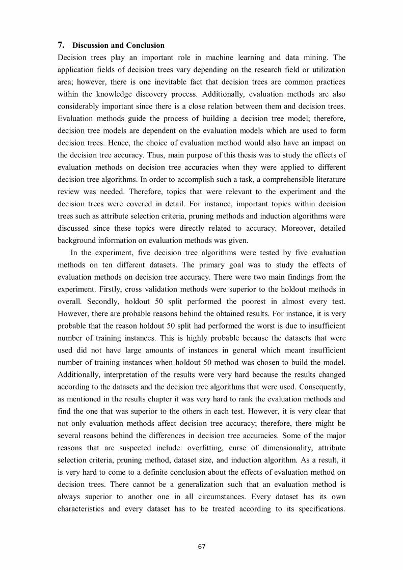
67
7. Discussion and Conclusion
Decision trees play an important role in machine learning and data mining. The
application fields of decision trees vary depending on the research field or utilization
area; however, there is one inevitable fact that decision trees are common practices
within the knowledge discovery process. Additionally, evaluation methods are also
considerably important since there is a close relation between them and decision trees.
Evaluation methods guide the process of building a decision tree model; therefore,
decision tree models are dependent on the evaluation models which are used to form
decision trees. Hence, the choice of evaluation method would also have an impact on
the decision tree accuracy. Thus, main purpose of this thesis was to study the effects of
evaluation methods on decision tree accuracies when they were applied to different
decision tree algorithms. In order to accomplish such a task, a comprehensible literature
review was needed. Therefore, topics that were relevant to the experiment and the
decision trees were covered in detail. For instance, important topics within decision
trees such as attribute selection criteria, pruning methods and induction algorithms were
discussed since these topics were directly related to accuracy. Moreover, detailed
background information on evaluation methods was given.
In the experiment, five decision tree algorithms were tested by five evaluation
methods on ten different datasets. The primary goal was to study the effects of
evaluation methods on decision tree accuracy. There were two main findings from the
experiment. Firstly, cross validation methods were superior to the holdout methods in
overall. Secondly, holdout 50 split performed the poorest in almost every test.
However, there are probable reasons behind the obtained results. For instance, it is very
probable that the reason holdout 50 split had performed the worst is due to insufficient
number of training instances. This is highly probable because the datasets that were
used did not have large amounts of instances in general which meant insufficient
number of training instances when holdout 50 method was chosen to build the model.
Additionally, interpretation of the results were very hard because the results changed
according to the datasets and the decision tree algorithms that were used. Consequently,
as mentioned in the results chapter it was very hard to rank the evaluation methods and
find the one that was superior to the others in each test. However, it is very clear that
not only evaluation methods affect decision tree accuracy; therefore, there might be
several reasons behind the differences in decision tree accuracies. Some of the major
reasons that are suspected include: overfitting, curse of dimensionality, attribute
selection criteria, pruning method, dataset size, and induction algorithm. As a result, it
is very hard to come to a definite conclusion about the effects of evaluation method on
decision trees. There cannot be a generalization such that an evaluation method is
always superior to another one in all circumstances. Every dataset has its own
characteristics and every dataset has to be treated according to its specifications.

68
Therefore, it is important to understand the data comprehensibly and chose the correct
evaluation method accordingly before building a decision tree model.
There were two limitations that were encountered in the thesis. First and most
importantly, the number of datasets that were tested was not sufficient. Therefore, the
experiment that was conducted was not very conclusive. Secondly, there were
difficulties when testing the datasets. The tools that were available did not have all the
necessary algorithms or the evaluation methods that were required for the experiment.
Therefore, it was hard to combine several tools in order to conduct the experiment.
Additionally, not all the tools available were open source. Thus, some important tools
were discarded due to lack of financial support.
For future work, a more comprehensible experiment with more datasets could be
made. Additionally, there were a few topics that were going to be tested but were
discarded in the later phases of the thesis. For instance, the total number of attributes
might also affect the accuracy of the decision trees. There are already solid findings in
the literature that the dimensionality affects accuracy but it would still be interesting to
test this notion on decision trees. Moreover, the effect of having different types of
attributes such as continuous, categorical or mixed might also affect accuracy of the
decision tree, so this issue could also be pursued. Lastly, dataset’s size might also have
effects on decision tree model’s accuracy. Hence, the datasets can be tested by taking
different proportions of the data using stratified sampling and the obtained results could
be analyzed to study the relation between the dataset size and decision tree accuracies
when built by different evaluation methods.

69
References
[Alpaydin, 2014] Alpaydin, E. (2014). Introduction to machine learning. MIT press.
[Bache and Lichman, 2015] Bache, K., and Lichman, M. (2015). {UCI} Machine
Learning Repository. Retrieved from http://archive.ics.uci.edu/ml
[Badulescu, 2007] Badulescu, L. A. (2007). The choice of the attribute selection
measure in Decision Tree induction. Annals of the University of Craiova-
Mathematics and Computer Science Series, 34, 88–93.
[Blumer et al., 1987] Blumer, A., Ehrenfeucht, A., Haussler, D., and Warmuth, M. K.
(1987). Occam’s razor. Information Processing Letters, 24(6), 377–380.
[Bouckaert et al., 2010] Bouckaert, R. R., Frank, E., Hall, M. A., Holmes, G.,
Pfahringer, B., Reutemann, P., and Witten, I. H. (2010). WEKA---Experiences
with a Java Open-Source Project. J.Mach.Learn.Res., 11, 2533–2541.
[Breiman et al., 1993] Breiman, L., Friedman, J. H., Olshen, R. A., and Stone, C. J.
(1993). Classification and Regression Trees, Wadsworth International Group,
Belmont, CA, 1984. Case Description Feature Subset Correct Missed FA
Misclass, 1, 1–3.
[Breiman et al., 1984] Breiman, L., Friedman, J., Stone, C. J., and Olshen, R. A. (1984).
Classification and regression trees. CRC press.
[Dietterich, 1994] Dietterich, T. (1994). Musk1 Dataset. Retrieved December 12, 2014,
from https://archive.ics.uci.edu/ml/datasets/Musk+(Version+1)
[Fayyad et al., 1996] Fayyad, U., Piatetsky-Shapiro, G., and Smyth, P. (1996). From
Data Mining to Knowledge Discovery in Databases.
[Fisher, 1988] Fisher, R. (1988). Iris Dataset. Retrieved December 12, 2014, from
https://archive.ics.uci.edu/ml/datasets/Iris
[Forsyth, 1990] Forsyth, R. (1990). Zoo Dataset. Retrieved December 12, 2014, from
https://archive.ics.uci.edu/ml/datasets/Zoo
[Frank, 2000] Frank, E. (2000). Pruning decision trees and lists. Citeseer. Retrieved
from
http://citeseerx.ist.psu.edu/viewdoc/download?doi=10.1.1.149.3509&rep=rep1&ty
pe=pdf
[German, 1987] German, B. (1987). Glass Identification Dataset. Retrieved December
12, 2014, from https://archive.ics.uci.edu/ml/datasets/Glass+Identification
[Gong, 1988] Gong, G. (1988). Hepatitis Dataset. Retrieved December 12, 2014, from
https://archive.ics.uci.edu/ml/datasets/Hepatitis
[Guvenir et al., 1998] Guvenir, A., Acar, B., and Muderrisoglu, H. (1998). Arrhythmia
Dataset. Retrieved December 02, 2014, from
https://archive.ics.uci.edu/ml/datasets/Arrhythmia
70
[Hall et al., 2009] Hall, M., Frank, E., Holmes, G., Pfahringer, B., Reutemann, P., and
Witten, I. H. (2009). The WEKA Data Mining Software: An Update. SIGKDD
Explor.Newsl., 11(1), 10–18.
[Han and Kamber, 2006] Han, J., and Kamber, M. (2006). Data Mining, Southeast Asia
Edition: Concepts and Techniques. Morgan kaufmann.
[Han et al., 2011] Han, J., Kamber, M., and Pei, J. (2011). Data Mining: Concepts and
Techniques (3rd ed.). San Francisco, CA, USA: Morgan Kaufmann Publishers Inc.
[Hand et al., 2001] Hand, D. J., Mannila, H., and Smyth, P. (2001). Principles of data
mining. MIT press.
[Hofmann and Klinkenberg, 2013] Hofmann, M., and Klinkenberg, R. (2013).
RapidMiner: Data mining use cases and business analytics applications. CRC
Press.
[Hssina et al., 2014] Hssina, B., Merbouha, A., Ezzikouri, H., and Erritali, M. (2014). A
comparative study of decision tree ID3 and C4. 5. International Journal of
Advanced Computer Science and Applications, 4(2).
[Hume, 1994] Hume, T. (1994). Balance Scale Dataset. Retrieved December 12, 2014,
from https://archive.ics.uci.edu/ml/datasets/Balance+Scale
[Hunt et al., 1966] Hunt, E. B., Marin, J., and Stone, P. J. (1966). Experiments in
induction.
[IBM, 2011] IBM. (2011). CHAID and Exhaustive CHAID Algorithms.
[IBM, 2014a] IBM. (2014a). IBM SPSS Modeler. Retrieved November 11, 2014, from
http://www-01.ibm.com/software/analytics/spss/products/modeler/
[IBM, 2014b] IBM. (2014b). IBM SPSS Modeler 16.0 Documentation. Retrieved
November 11, 2014, from
ftp://public.dhe.ibm.com/software/analytics/spss/documentation/modeler/16.0/en/
AlgorithmsGuide.pdf
[Iltanen, 2014] Iltanen, K. (2014). Decision Tree Induction 2. Retrieved November 11,
2014, from http://www.sis.uta.fi/~cskavi/timus14/lectures/classification_dt/
[Jackson, 2002] Jackson, J. (2002). Data Mining; A Conceptual Overview.
Communications of the Association for Information Systems, 8(1), 19.
[Jergen, 1992] Jergen, P. (1992). Audiology (Standadized) Dataset. Retrieved December
03, 2014, from https://archive.ics.uci.edu/ml/datasets/Audiology+(Standardized)
[Kantardzic, 2011] Kantardzic, M. (2011). Data mining: concepts, models, methods,
and algorithms. John Wiley & Sons.
[Karabadji et al., 2014] Karabadji, N. E. I., Seridi, H., Khelf, I., Azizi, N., and
Boulkroune, R. (2014). Improved decision tree construction based on attribute
selection and data sampling for fault diagnosis in rotating machines. Engineering
71
Applications of Artificial Intelligence, 35(0), 71–83. Retrieved from
http://www.sciencedirect.com/science/article/pii/S0952197614001328
[Kass, 1980] Kass, G. V. (1980). An exploratory technique for investigating large
quantities of categorical data. Applied Statistics, 119–127.
[Lai et al., 2007] Lai, C.-C., Doong, S.-H., and Wu, C.-H. (2007). Machine Learning. In
Wiley Encyclopedia of Computer Science and Engineering. John Wiley & Sons,
Inc. Retrieved from http://dx.doi.org/10.1002/9780470050118.ecse228
[Loh, 2011] Loh, W.-Y. (2011). Classification and regression trees. Wiley
Interdisciplinary Reviews: Data Mining and Knowledge Discovery, 1(1), 14–23.
Retrieved from http://dx.doi.org/10.1002/widm.8
[Maimon and Rokach, 2005] Maimon, O. Z., and Rokach, L. (2005). Data mining and
knowledge discovery handbook (Vol. 1). Springer.
[Mingers, 1989] Mingers, J. (1989). An empirical comparison of selection measures for
decision-tree induction. Machine Learning, 3(4), 319–342.
[Mitchell, 1997] Mitchell, T. (1997). Decision tree learning. Machine Learning, 414.
[Mosley Jr, 2012] Mosley Jr, R. C. (2012). Social media analytics: Data mining applied
to insurance Twitter posts. In Casualty Actuarial Society E-Forum, Winter 2012
Volume 2 (p. 1).
[Niblett and Bratko, 1987] Niblett, T., and Bratko, I. (1987). Learning decision rules in
noisy domains. In Proceedings of Expert Systems’ 86, The 6Th Annual Technical
Conference on Research and development in expert systems III (pp. 25–34).
Cambridge University Press.
[Olson and Delen, 2008] Olson, D. L., and Delen, D. (2008). Advanced data mining
techniques. Springer Science & Business Media.
[Quinlan, 1986] Quinlan, J. R. (1986). Induction of decision trees. Machine Learning,
1(1), 81–106.
[Quinlan, 1987] Quinlan, J. R. (1987). Simplifying decision trees. International Journal
of Man-Machine Studies, 27(3), 221–234.
[Quinlan, 1993] Quinlan, J. R. (1993). C4. 5: programs for machine learning (Vol. 1).
Morgan kaufmann.
[Quinlan, 2004] Quinlan, J. R. (2004). Data mining tools See5 and C5. 0.
[Rokach and Maimon, 2014] Rokach, L., and Maimon, O. (2014). Data mining with
decision trees: theory and applications. 2nd Edition (Vol. 69). World scientific.
[Shalizi, 2009] Shalizi, C. (2009). Classification and Regression Trees 36-350,
(November). Retrieved from
http://www.stat.cmu.edu/~cshalizi/350/lectures/22/lecture-22.pdf

72
[Shannon, 1951] Shannon, C. E. (1951). Prediction and entropy of printed English. Bell
System Technical Journal, 30(1), 50–64.
[Sigillito, 1989] Sigillito, V. (1989). Ionosphere Dataset. Retrieved December 12, 2014,
from https://archive.ics.uci.edu/ml/datasets/Ionosphere
[Tan et al., 2006] Tan, P.-N., Steinbach, M., and Kumar, V. (2006). Classification :
Basic Concepts , Decision Trees , and. Introduction to Data Mining, 67, 145–205.
doi:10.1016/0022-4405(81)90007-8
[Turing, 1950] Turing, A. M. (1950). Computing machinery and intelligence. Mind,
433–460.
[Varpa et al., 2008] Varpa, K., Iltanen, K., and Juhola, M. (2008). Machine learning
method for knowledge discovery experimented with otoneurological data.
Computer Methods and Programs in Biomedicine, 91(2), 154–164.
[Witten et al., 2011] Witten, I. H., Frank, E., Hall, M. a., and Mark, A. (2011). Hall
(2011)." Data Mining: Practical machine learning tools and techniques.
Complementary literature None (p. 664). Morgan Kaufmann, San Francisco.
Retrieved. Retrieved from
http://books.google.com/books?id=bDtLM8CODsQC&pgis=1
[Zwitter and Soklic, 1988] Zwitter, M., and Soklic, M. (1988). Breast Cancer Dataset.
Retrieved December 12, 2014, from
https://archive.ics.uci.edu/ml/datasets/Breast+Cancer