babu ram dawadi1 decision tree: outline decision tree representation decision tree representation...
TRANSCRIPT

Babu Ram DawadiBabu Ram Dawadi 11
Decision Tree: OutlineDecision Tree: Outline
Decision tree representationDecision tree representation ID3 learning algorithmID3 learning algorithm Entropy, information gainEntropy, information gain OverfittingOverfitting

Babu Ram DawadiBabu Ram Dawadi 22
Defining the TaskDefining the Task
Imagine we’ve got a set of data containing Imagine we’ve got a set of data containing several types, or several types, or classesclasses.. E.g. information about customers, and E.g. information about customers, and
class=whether or not they buy anything.class=whether or not they buy anything.
Can we predict, i.e Can we predict, i.e classifyclassify, whether a , whether a previously unseen customer will buy previously unseen customer will buy something?something?

33
An Example Decision TreeAn Example Decision Tree
We create a ‘We create a ‘decision treedecision tree’. It acts like ’. It acts like a function that can predict and a function that can predict and output given an inputoutput given an input
Attributen
AttributemAttributek
Attributel
vn1vn2
vn3
vm1 vm2
vl1 vl2
vk1 vk2Class1
Class2 Class2
Class2Class1
Class1

Babu Ram DawadiBabu Ram Dawadi 44
Decision TreesDecision Trees
The idea is to The idea is to ask a series of questionsask a series of questions, , starting at the root, that will lead to a leaf starting at the root, that will lead to a leaf node.node.
The The leaf node provides the classificationleaf node provides the classification..

55
Classification by Decision Tree InductionClassification by Decision Tree Induction Decision tree Decision tree
A flow-chart-like tree structureA flow-chart-like tree structure Internal node denotes a test on an attributeInternal node denotes a test on an attribute Branch represents an outcome of the testBranch represents an outcome of the test Leaf nodes represent class labels or class distributionLeaf nodes represent class labels or class distribution
Decision tree generation consists of two phasesDecision tree generation consists of two phases Tree constructionTree construction
At start, all the training examples are at the rootAt start, all the training examples are at the root Partition examples recursively based on selected attributesPartition examples recursively based on selected attributes
Tree pruningTree pruning Identify and remove branches that reflect noise or outliersIdentify and remove branches that reflect noise or outliers
Once the tree is build Once the tree is build Use of decision tree: Classifying an unknown sampleUse of decision tree: Classifying an unknown sample

66
Decision Tree for PlayTennisDecision Tree for PlayTennis
Outlook
Sunny Overcast Rain
Humidity
High Normal
Wind
Strong Weak
No Yes
Yes
YesNo

77
Decision Tree for PlayTennisDecision Tree for PlayTennis
Outlook
Sunny Overcast Rain
Humidity
High Normal
No Yes
Each internal node tests an attribute
Each branch corresponds to anattribute value node
Each leaf node assigns a classification

88
No
Decision Tree for PlayTennisDecision Tree for PlayTennis
Outlook
Sunny Overcast Rain
Humidity
High Normal
Wind
Strong Weak
No Yes
Yes
YesNo
Outlook Temperature Humidity Wind PlayTennis Sunny Hot High Weak ?

99
Decision TreesDecision Trees
Consider these Consider these data:data:
A number of A number of examples of examples of weather, for weather, for several days, several days, with a with a classification classification ‘PlayTennis.’‘PlayTennis.’

1010
Decision Tree AlgorithmDecision Tree Algorithm
Building a decision treeBuilding a decision tree1.1. Select an attributeSelect an attribute2.2. Create the subsets of the example data Create the subsets of the example data
for each value of the attributefor each value of the attribute3.3. For each subsetFor each subset
• if not all the elements of the subset if not all the elements of the subset belongs to same class repeat the belongs to same class repeat the steps 1-3 for the subsetsteps 1-3 for the subset

Babu Ram DawadiBabu Ram Dawadi 1111
Building Decision TreesBuilding Decision Trees
Let’s start building the tree from scratch. We first need to decide which attribute to make a decision. Let’s say we selected “humidity”
Humidity
high normal
D1,D2,D3,D4D8,D12,D14
D5,D6,D7,D9D10,D11,D13

1212
Building Decision TreesBuilding Decision Trees
Now lets classify the first subset D1,D2,D3,D4,D8,D12,D14 using attribute “wind”
Humidity
high normal
D1,D2,D3,D4D8,D12,D14
D5,D6,D7,D9D10,D11,D13

1313
Building Decision TreesBuilding Decision Trees
Subset D1,D2,D3,D4,D8,D12,D14 classified by attribute “wind”
Humidity
high normal
D5,D6,D7,D9D10,D11,D13
wind
strong weak
D1,D3,D4,D8D2,D12,D14

1414
Building Decision TreesBuilding Decision Trees
Now lets classify the subset D2,D12,D14 using attribute “outlook”
Humidity
high normal
D5,D6,D7,D9D10,D11,D13
wind
strong weak
D1,D3,D4,D8D2,D12,D14

1515
Building Decision TreesBuilding Decision Trees
Subset D2,D12,D14 classified by “outlook”
Humidity
high normal
D5,D6,D7,D9D10,D11,D13
wind
strong weak
D1,D3,D4,D8D2,D12,D14

1616
Building Decision TreesBuilding Decision Trees
subset D2,D12,D14 classified using attribute “outlook”
Humidity
high normal
D5,D6,D7,D9D10,D11,D13
wind
strong weak
D1,D3,D4,D8outlook
Sunny Rain Overcast
YesNo No

1717
Building Decision TreesBuilding Decision Trees
Humidity
high normal
D5,D6,D7,D9D10,D11,D13
wind
strong weak
D1,D3,D4,D8outlook
Sunny Rain Overcast
YesNo No
Now lets classify the subset D1,D3,D4,D8 using attribute “outlook”

1818
Building Decision TreesBuilding Decision Trees
Humidity
high normal
D5,D6,D7,D9D10,D11,D13
wind
strong weak
outlook
Sunny Rain Overcast
YesNo No
subset D1,D3,D4,D8 classified by “outlook”
outlook
Sunny Rain Overcast
YesNo Yes

1919
Building Decision TreesBuilding Decision Trees
Humidity
high normal
D5,D6,D7,D9D10,D11,D13
wind
strong weak
outlook
Sunny Rain Overcast
YesNo No
Now classify the subset D5,D6,D7,D9,D10,D11,D13 using attribute “outlook”
outlook
Sunny Rain Overcast
YesNo Yes

2020
Building Decision TreesBuilding Decision Trees
Humidity
high normal
wind
strong weak
outlook
Sunny Rain Overcast
YesNo No
subset D5,D6,D7,D9,D10,D11,D13 classified by “outlook”
outlook
Sunny Rain Overcast
YesNo Yes
outlook
Sunny Rain Overcast
YesYes D5,D6,D10

2121
Building Decision TreesBuilding Decision Trees
Humidity
high normal
wind
strong weak
outlook
Sunny Rain Overcast
YesNo No
Finally classify subset D5,D6,D10by “wind”
outlook
Sunny Rain Overcast
YesNo Yes
outlook
Sunny Rain Overcast
YesYes D5,D6,D10

2222
Building Decision TreesBuilding Decision Trees
Humidity
high normal
wind
strong weak
outlook
Sunny Rain Overcast
YesNo No
subset D5,D6,D10 classified by “wind”
outlook
Sunny Rain Overcast
YesNo Yes
outlook
Sunny Rain Overcast
YesYes wind
strong weak
YesNo

2323
Decision Trees and LogicDecision Trees and Logic
Humidity
high normal
wind
strong weak
outlook
Sunny Rain Overcast
YesNo No
(humidity=high (humidity=high wind=strong wind=strong outlook=overcast) outlook=overcast) (humidity=high (humidity=high wind=weak wind=weak outlook=overcast) outlook=overcast) (humidity=normal (humidity=normal outlook=sunny) outlook=sunny) (humidity=normal (humidity=normal outlook=overcast) outlook=overcast) (humidity=normal (humidity=normal outlook=rain outlook=rain wind=weak) wind=weak) ‘Yes’ ‘Yes’
outlook
Sunny Rain Overcast
YesNo Yes
outlook
Sunny Rain Overcast
YesYes wind
strong weak
YesNo
The decision tree can be expressed The decision tree can be expressed as an expression or if-then-else as an expression or if-then-else sentences:sentences:

2424
Using Decision TreesUsing Decision Trees
Humidity
high normal
wind
strong weak
outlook
Sunny Rain Overcast
YesNo No
Now let’s classify an unseen example: <sunny,hot,normal,weak>=?Now let’s classify an unseen example: <sunny,hot,normal,weak>=?
outlook
Sunny Rain Overcast
YesNo Yes
outlook
Sunny Rain Overcast
YesYes wind
strong weak
YesNo

2525
Using Decision TreesUsing Decision Trees
Classifying: <sunny,hot,Classifying: <sunny,hot,normalnormal,weak>=?,weak>=?
Humidity
high normal
wind
strong weak
outlook
Sunny Rain Overcast
YesNo No
outlook
Sunny Rain Overcast
YesNo Yes
Rain Overcast
Yeswind
strong weak
YesNo
outlook
Sunny
Yes

2626
Using Decision TreesUsing Decision Trees
Classification for: <Classification for: <sunnysunny,hot,,hot,normalnormal,weak>=Yes,weak>=Yes
Humidity
high normal
wind
strong weak
outlook
Sunny Rain Overcast
YesNo No
outlook
Sunny Rain Overcast
YesNo Yes
outlook
Sunny Rain Overcast
YesYes wind
strong weak
YesNo

2727
A Big Problem…A Big Problem…
Here’s another tree from the Here’s another tree from the same training same training datadata that has a different attribute order: that has a different attribute order:
Which attribute should we choose for each branch?Which attribute should we choose for each branch?

2828
Choosing AttributesChoosing Attributes
We need a way of We need a way of choosing the bestchoosing the best attributeattribute each time we add a node to the tree.each time we add a node to the tree.
Most commonly we use a measure called Most commonly we use a measure called entropyentropy..
Entropy measure the degree of Entropy measure the degree of disorderdisorder in a in a set of objects.set of objects.

2929
EntropyEntropy In our system we have In our system we have
9 positive examples9 positive examples 5 negative examples5 negative examples
The The entropy, E(S),entropy, E(S), of a set of a set of examples is:of examples is: E(S) = E(S) = -p-pii log p log pii
Where c = no of classes and pWhere c = no of classes and p i i
= ratio of the number of = ratio of the number of examples of this value over examples of this value over the total number of examples.the total number of examples.
P+ = 9/14P+ = 9/14 P- = 5/14P- = 5/14 E = - 9/14 logE = - 9/14 log22 9/14 - 5/14 log 9/14 - 5/14 log22 5/14 5/14
E = E = 0.9400.940
- In a - In a homogenoushomogenous (totally (totally ordered) system, the entropy is ordered) system, the entropy is 0. 0.
- In a - In a totallytotally heterogeneousheterogeneous system (totally disordered), all system (totally disordered), all classes have equal numbers of classes have equal numbers of instances; the entropy is 1instances; the entropy is 1
i=1i=1
cc

3030
EntropyEntropy
We can evaluate We can evaluate each each attributeattribute for their entropy. for their entropy. E.g. evaluate the attribute E.g. evaluate the attribute
““TemperatureTemperature”” Three values: ‘Hot’, ‘Mild’, Three values: ‘Hot’, ‘Mild’,
‘Cool.’‘Cool.’
So we have three subsets, So we have three subsets, one for each value of one for each value of ‘Temperature’.‘Temperature’.
SShothot={D1,D2,D3,D13}={D1,D2,D3,D13}
SSmildmild={D4,D8,D10,D11,D12,D14}={D4,D8,D10,D11,D12,D14}
SScoolcool={D5,D6,D7,D9}={D5,D6,D7,D9}
We will now find:We will now find: E(SE(Shothot))
E(SE(Smildmild))
E(SE(Scoolcool))

3131
EntropyEntropy
Shot= {D1,D2,D3,D13}
Examples:2 positive 2 negative
Totally heterogeneous + disordered therefore:p+= 0.5p-= 0.5
Entropy(Shot),=-0.5log20.5
-0.5log20.5 = 1.0
Smild= {D4,D8,D10, D11,D12,D14} Examples:4 positive2 negative
Proportions of each class in this subset:p+= 0.666p-= 0.333
Entropy(Smild),=-0.666log20.666
-0.333log20.333 = 0.918
Scool={D5,D6,D7,D9}
Examples:3 positive1 negative
Proportions of each class in this subset:p+= 0.75p-= 0.25
Entropy(Scool),=-0.25log20.25
-0.75log20.75 = 0.811

3232
GainGain
Now we can compare the entropy of the system Now we can compare the entropy of the system beforebefore we divided we divided it into subsets using “Temperature”, with the entropy of the it into subsets using “Temperature”, with the entropy of the system system afterwardsafterwards. This will tell us how good “Temperature” is . This will tell us how good “Temperature” is as an attribute.as an attribute.
The entropy of the system after we use attribute “Temperature” The entropy of the system after we use attribute “Temperature” is:is:
(|S(|Shothot|/|S|)*E(S|/|S|)*E(Shothot) + (|S) + (|Smildmild|/|S|)*E(S|/|S|)*E(Smildmild) + (|S) + (|Scoolcool|/|S|)*E(S|/|S|)*E(Scoolcool))
This difference between the entropy of the system before and This difference between the entropy of the system before and after the split into subsets is called the after the split into subsets is called the gaingain::
(4/14)*1.0 + (6/14)*0.918 + (4/14)*0.811 = (4/14)*1.0 + (6/14)*0.918 + (4/14)*0.811 = 0.91080.9108
Gain(S,Temperature) = 0.940 - 0.9108 = Gain(S,Temperature) = 0.940 - 0.9108 = 0.0290.029
E(before) E(afterwards)

3333
Decreasing EntropyDecreasing Entropy
7red class 7pink class: E=1.0All subset: E=0.0Both subsets
E=-2/7log2/7 –5/7log5/7
Has
a c
ross
?
Has
a r
ing?
Has
a r
ing?
no
no
no
yes
yes
yes
From the initial state,Where there is total disorder…
…to the final state where all subsets contain a single class

3434
Tabulating the PossibilitiesTabulating the Possibilities
Attribute=valueAttribute=value |+||+| |-||-| EE E after dividing E after dividing by attribute Aby attribute A
GainGain
Outlook=sunnyOutlook=sunny 22 33 -2/5 log 2/5 – 3/5 log 3/5 = 0.9709-2/5 log 2/5 – 3/5 log 3/5 = 0.9709 0.69350.6935 0.24650.2465
Outlook=o’castOutlook=o’cast 44 00 -4/4 log 4/4 – 0/4 log 0/4 = 0.0-4/4 log 4/4 – 0/4 log 0/4 = 0.0
Outlook=rainOutlook=rain 33 22 -3/5 log 3/5 – 2/5 log 2/5 = 0.9709-3/5 log 3/5 – 2/5 log 2/5 = 0.9709
Temp’=hotTemp’=hot 22 22 -2/2 log 2/2 – 2/2 log 2/2 = 1.0-2/2 log 2/2 – 2/2 log 2/2 = 1.0 0.91080.9108 0.02920.0292
Temp’=mildTemp’=mild 44 22 -4/6 log 4/6 – 2/6 log 2/6 = 0.9183-4/6 log 4/6 – 2/6 log 2/6 = 0.9183
Temp’=coolTemp’=cool 33 11 -3/4 log 3/4 – 1/4 log 1/4 = 0.8112-3/4 log 3/4 – 1/4 log 1/4 = 0.8112
Etc…Etc…
… etc This shows the entropy calculations…
3535
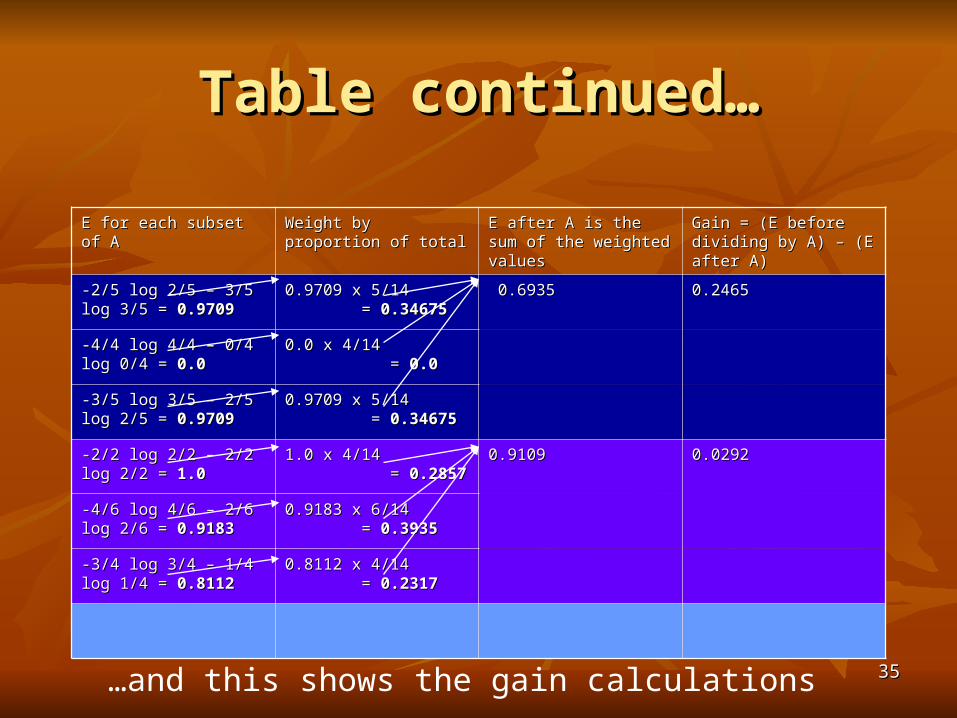
Table continued…Table continued…
E for each subset of AE for each subset of A Weight by proportion of Weight by proportion of totaltotal
E after A is the sum of the E after A is the sum of the weighted valuesweighted values
Gain = (E before dividing Gain = (E before dividing by A) – (E after A)by A) – (E after A)
-2/5 log 2/5 – 3/5 log 3/5 = -2/5 log 2/5 – 3/5 log 3/5 = 0.97090.9709
0.9709 x 5/14 = 0.9709 x 5/14 = 0.346750.34675
0.69350.6935 0.24650.2465
-4/4 log 4/4 – 0/4 log 0/4 = -4/4 log 4/4 – 0/4 log 0/4 = 0.00.0
0.0 x 4/14 = 0.0 x 4/14 = 0.00.0
-3/5 log 3/5 – 2/5 log 2/5 = -3/5 log 3/5 – 2/5 log 2/5 = 0.97090.9709
0.9709 x 5/14 = 0.9709 x 5/14 = 0.346750.34675
-2/2 log 2/2 – 2/2 log 2/2 = -2/2 log 2/2 – 2/2 log 2/2 = 1.01.0
1.0 x 4/14 = 1.0 x 4/14 = 0.28570.2857
0.91090.9109 0.02920.0292
-4/6 log 4/6 – 2/6 log 2/6 = -4/6 log 4/6 – 2/6 log 2/6 = 0.91830.9183
0.9183 x 6/14 = 0.9183 x 6/14 = 0.39350.3935
-3/4 log 3/4 – 1/4 log 1/4 = -3/4 log 3/4 – 1/4 log 1/4 = 0.81120.8112
0.8112 x 4/14 = 0.8112 x 4/14 = 0.23170.2317
…and this shows the gain calculations

3636
GainGain
We calculate the gain We calculate the gain for all the attributes.for all the attributes.
Then we see which of Then we see which of them will bring more them will bring more ‘order’ to the set of ‘order’ to the set of examples.examples.
Gain(S,Outlook) = Gain(S,Outlook) = 0.2460.246 Gain(S,Humidity) = 0.151Gain(S,Humidity) = 0.151 Gain(S,Wind) = 0.048Gain(S,Wind) = 0.048 Gain(S, Temp’) = 0.029Gain(S, Temp’) = 0.029
The first node in the tree The first node in the tree should be the one with should be the one with the highest value, i.e. the highest value, i.e. ‘‘Outlook’Outlook’..

3737
ID3 (Decision Tree Algorithm: ID3 (Decision Tree Algorithm: (Quinlan 1979)(Quinlan 1979)))
ID3 was the first proper decision tree ID3 was the first proper decision tree algorithm to use this mechanism:algorithm to use this mechanism:
Building a decision tree with ID3 algorithm1. Select the attribute with the most gain2. Create the subsets for each value of the attribute3. For each subset
1. if not all the elements of the subset belongs to same class repeat the steps 1-3 for the subset
Main Hypothesis of ID3:Main Hypothesis of ID3: The The simplest treesimplest tree that that classifies training examples will work best on future classifies training examples will work best on future examples (Occam’s Razor)examples (Occam’s Razor)

3838
ID3 (Decision Tree Algorithm)ID3 (Decision Tree Algorithm)
•Function DecisionTtreeLearner(Function DecisionTtreeLearner(Examples, TargetClass, Attributes)Examples, TargetClass, Attributes) •create a create a Root node for the treeRoot node for the tree •ifif all all Examples are positive, Examples are positive, returnreturn the single-node tree the single-node tree Root, with label = Yes Root, with label = Yes •ifif all all Examples are negative, Examples are negative, returnreturn the single-node tree the single-node tree Root, with label = No Root, with label = No •ifif Attributes list is empty,Attributes list is empty,
• returnreturn the single-node tree the single-node tree Root, with label = most common value of TargetClass in Examples Root, with label = most common value of TargetClass in Examples •elseelse
•A =A = the attribute from the attribute from Attributes with the highest information gain with respect to Examples Attributes with the highest information gain with respect to Examples •Make Make A the decision attribute for Root A the decision attribute for Root •forfor each possible value each possible value v of A:v of A:
•add a new tree branch below add a new tree branch below Root, corresponding to the test A = v Root, corresponding to the test A = v •let let Examplesv be the subset of Examples that have value v for attribute A Examplesv be the subset of Examples that have value v for attribute A •ifif Examplesv is empty Examplesv is empty thenthen
•add a leaf node below this new branch with label = most common value of add a leaf node below this new branch with label = most common value of TargetClass in TargetClass in ExamplesExamples
•elseelse •add the subtree DTL(add the subtree DTL(Examplesv, TargetClass, Attributes - { A })Examplesv, TargetClass, Attributes - { A })
•end ifend if•endend•returnreturn Root Root

3939
The Problem of OverfittingThe Problem of Overfitting
Trees may grow to Trees may grow to include include irrelevant irrelevant attributesattributes
NoiseNoise may add may add spurious nodesspurious nodes to the to the tree.tree.
This can cause This can cause overfitting overfitting ofof the the training data training data relative relative toto test data. test data. Hypothesis Hypothesis H H overfitsoverfits the data if there exists the data if there exists
H’ H’ with greater error than with greater error than HH, over training , over training examples, but less error than examples, but less error than HH over entire over entire
distribution of instances. distribution of instances.

4040
Fixing Over-fittingFixing Over-fitting
Two approaches to pruning
Prepruning: Stop growing tree during the training when it is determined that there is not enough data to make reliable choices.
Postpruning: Grow whole tree but then remove the branches that do not contribute good overall performance.

4141
Rule Post-PruningRule Post-PruningRule post-pruning
•prune (generalize) each rule by removing any preconditions (i.e., attribute tests) that result in improving its accuracy over the validation set
•sort pruned rules by accuracy, and consider them in this order when classifying subsequent instances
•IF (Outlook = Sunny) ^ (Humidity = High) THEN PlayTennis = No
•Try removing (Outlook = Sunny) condition or (Humidity = High) condition from the rule and select whichever pruning step leads to the biggest improvement in accuracy on the validation set (or else neither if no improvement results).
•converting to rules improves readability

4242
Advantage and Disadvantages of Decision TreesAdvantage and Disadvantages of Decision Trees
Advantages:Advantages: Easy to understand and map nicely to a production rulesEasy to understand and map nicely to a production rules Suitable for categorical as well as numerical inputsSuitable for categorical as well as numerical inputs No statistical assumptions about distribution of attributesNo statistical assumptions about distribution of attributes Generation and application to classify unknown outputs is very fastGeneration and application to classify unknown outputs is very fast
Disadvantages:Disadvantages: Output attributes must be categoricalOutput attributes must be categorical Unstable: slight variations in the training data may result in different Unstable: slight variations in the training data may result in different
attribute selections and hence different treesattribute selections and hence different trees Numerical input attributes leads to complex trees as attribute splits Numerical input attributes leads to complex trees as attribute splits
are usually binaryare usually binary

4343
HomeworkHomework
age income student credit_rating buys_computer<=30 high no fair no<=30 high no excellent no31…40 high no fair yes>40 medium no fair yes>40 low yes fair yes>40 low yes excellent no31…40 low yes excellent yes<=30 medium no fair no<=30 low yes fair yes>40 medium yes fair yes<=30 medium yes excellent yes31…40 medium no excellent yes31…40 high yes fair yes>40 medium no excellent no
Given the training data set, to identify whether a customer buys computer or not, Develop a Decision Tree using ID3 technique.

4444
Association RulesAssociation Rules
Example1:Example1: a female shopper buys a handbag is a female shopper buys a handbag is likely to buy shoeslikely to buy shoes
Example2Example2: when a male customer buys beer, he is : when a male customer buys beer, he is likely to buy salted peanutslikely to buy salted peanuts
It is not very difficult to develop algorithms that It is not very difficult to develop algorithms that will find this associations in a large databasewill find this associations in a large database The problem is that such an algorithm will also uncover The problem is that such an algorithm will also uncover
many other associations that are of very little value.many other associations that are of very little value.

4545
Association RulesAssociation Rules It is necessary to introduce some measures to distinguish It is necessary to introduce some measures to distinguish
interesting associations from non-interesting onesinteresting associations from non-interesting ones
Look for associations that have a lots of examples in the Look for associations that have a lots of examples in the database: support of an association ruledatabase: support of an association rule
May be that a considerable group of people who read all three May be that a considerable group of people who read all three magazines but there is a much larger group that buys A & B, magazines but there is a much larger group that buys A & B, but not C; association is very weak here although support but not C; association is very weak here although support might be very high.might be very high.

4646
Associations….Associations…. Percentage of records for which C holds, within the Percentage of records for which C holds, within the
group of records for which A & B hold: group of records for which A & B hold: confidenceconfidence
Association rules are only useful in data mining if we Association rules are only useful in data mining if we already have a rough idea of what is we are looking already have a rough idea of what is we are looking for.for.
We will represent an association rule in the following We will represent an association rule in the following way:way: MUSIC_MAG, HOUSE_MAG=>CAR_MAGMUSIC_MAG, HOUSE_MAG=>CAR_MAG Somebody that reads both a music and a house magazine is also very likely to Somebody that reads both a music and a house magazine is also very likely to
read a car magazineread a car magazine

Babu Ram DawadiBabu Ram Dawadi 4747
Associations…Associations…
Example: shopping Basket analysisExample: shopping Basket analysis
TransactionsTransactions ChipsChips RasbariRasbari SamosaSamosa CokeCoke TeaTea
T1T1 XX XX
T2T2 XX XX
T3T3 XX XX XX

4848
Example…Example… 1. find all frequent Itemsets:1. find all frequent Itemsets: (a) 1-itemsets(a) 1-itemsets
K= [{Chips}C=1,{Rasbari}C=3,{Samosa}C=2, K= [{Chips}C=1,{Rasbari}C=3,{Samosa}C=2, {Tea}C=1]{Tea}C=1]
(b) extend to 2-itemsets:(b) extend to 2-itemsets: L=[{Chips, Rasbari}C=1, {Rasbari,Samosa}C=2,L=[{Chips, Rasbari}C=1, {Rasbari,Samosa}C=2,
{Rasbari,Tea}C=1,{Samosa,Tea}C=1]{Rasbari,Tea}C=1,{Samosa,Tea}C=1] (c) Extend to 3-Itemsets:(c) Extend to 3-Itemsets:
M=[{Rasbari, Samosa,Tea}C=1M=[{Rasbari, Samosa,Tea}C=1

4949
Examples..Examples.. Match with the requirements:Match with the requirements:
Min. Support is 2 (66%)Min. Support is 2 (66%) (a) >> K1={{Rasbari}, {Samosa}}(a) >> K1={{Rasbari}, {Samosa}} (b) >>L1={Rasbari,Samosa}(b) >>L1={Rasbari,Samosa} (c) >>M1={}(c) >>M1={}
Build All possible rules:Build All possible rules: (a) no rule(a) no rule (b) >> possible rules:(b) >> possible rules:
Rasbari=>SamosaRasbari=>Samosa Samosa=>RasbariSamosa=>Rasbari
(c) No rule(c) No rule Support:Support: given the association rule X1,X2…Xn=>Y, the support is the Percentage given the association rule X1,X2…Xn=>Y, the support is the Percentage
of records for which X1,X2…Xn and Y both hold true.of records for which X1,X2…Xn and Y both hold true.

5050
Example..Example.. Calculate Confidence for b:Calculate Confidence for b:
Confidence of [Rasbari=>Samosa]Confidence of [Rasbari=>Samosa] {Rasbari,Samosa}C=2/{Rasbari}C=3{Rasbari,Samosa}C=2/{Rasbari}C=3 =2/3=2/3 66%66%
Confidence of Samosa=> RasbariConfidence of Samosa=> Rasbari {Rasbari,Samosa}C=2/{Samosa}C=2{Rasbari,Samosa}C=2/{Samosa}C=2 =2/2=2/2 100%100%
ConfidenceConfidence: Given the association rule X1,X2….Xn=>Y, the confidence is : Given the association rule X1,X2….Xn=>Y, the confidence is the percentage of records for which Y holds within the group of records for the percentage of records for which Y holds within the group of records for which X1,X2…Xn holds true.which X1,X2…Xn holds true.

5151
The A-Priori AlgorithmThe A-Priori Algorithm Set the threshold for Set the threshold for supportsupport rather high – to focus on a small number of best rather high – to focus on a small number of best
candidates, candidates,
Observation:Observation: If a set of items X has support s, then each subset of X must also If a set of items X has support s, then each subset of X must also have support at least shave support at least s..
( if a pair {i,j} appears in say, 1000 baskets, then we know there are at least 1000 ( if a pair {i,j} appears in say, 1000 baskets, then we know there are at least 1000 baskets with item i and at least 1000 baskets with item j )baskets with item i and at least 1000 baskets with item j )
Algorithm:Algorithm:
1)1) Find the set of candidate items – those that appear in a sufficient number of Find the set of candidate items – those that appear in a sufficient number of baskets by themselvesbaskets by themselves
2)2) Run the query on only the candidate itemsRun the query on only the candidate items

5252
Apriori AlgorithmApriori Algorithm
Scan the database and count the frequency of the candidate item-sets, then Large Item-sets are decided based on the user specified min_sup.
Based on the Large Item-sets, expand them with one more item to generate new Candidate item-sets.
Initialise the candidate Item-sets as single items in database.
Any new LargeItem-sets?
Stop
Begin
NO
YES

5353
Apriori: A Candidate Generation-and-test ApproachApriori: A Candidate Generation-and-test Approach
Any subset of a frequent itemset must be frequentAny subset of a frequent itemset must be frequent if if {beer, diaper, nuts}{beer, diaper, nuts} is frequent, so is is frequent, so is {beer, diaper}{beer, diaper} Every transaction having {beer, diaper, nuts} also contains Every transaction having {beer, diaper, nuts} also contains
{beer, diaper}{beer, diaper}
Apriori pruning principleApriori pruning principle: : If there is If there is anyany itemset which is itemset which is infrequent, its superset should not be generated/tested!infrequent, its superset should not be generated/tested!
The performance studies show its efficiency and The performance studies show its efficiency and scalabilityscalability

5454
The Apriori Algorithm — An ExampleThe Apriori Algorithm — An Example
Database TDB
1st scan
C1L1
L2
C2 C2
2nd scan
C3 L33rd scan
TidTid ItemsItems
1010 A, C, DA, C, D
2020 B, C, EB, C, E
3030 A, B, C, EA, B, C, E
4040 B, EB, E
ItemsetItemset supsup
{A}{A} 22
{B}{B} 33
{C}{C} 33
{D}{D} 11
{E}{E} 33
ItemsetItemset supsup
{A}{A} 22
{B}{B} 33
{C}{C} 33
{E}{E} 33
ItemsetItemset
{A, B}{A, B}
{A, C}{A, C}
{A, E}{A, E}
{B, C}{B, C}
{B, E}{B, E}
{C, E}{C, E}
ItemsetItemset supsup
{A, B}{A, B} 11
{A, C}{A, C} 22
{A, E}{A, E} 11
{B, C}{B, C} 22
{B, E}{B, E} 33
{C, E}{C, E} 22
ItemsetItemset supsup
{A, C}{A, C} 22
{B, C}{B, C} 22
{B, E}{B, E} 33
{C, E}{C, E} 22
ItemsetItemset
{B, C, E}{B, C, E}ItemsetItemset supsup
{B, C, E}{B, C, E} 22

5555
Problems with Problems with A-prioriA-priori Algorithms Algorithms
It is costly to handle a huge number of candidate sets. For example if It is costly to handle a huge number of candidate sets. For example if there are 10there are 1044 large 1-itemsets, the Apriori algorithm will need to large 1-itemsets, the Apriori algorithm will need to generate more than 10generate more than 1077 candidate 2-itemsets. Moreover for 100- candidate 2-itemsets. Moreover for 100-itemsets, it must generate more than 2itemsets, it must generate more than 2100100 10 103030 candidates in total. candidates in total.
The candidate generation is the The candidate generation is the inherent costinherent cost of the Apriori of the Apriori Algorithms, no matter what implementation technique is applied.Algorithms, no matter what implementation technique is applied.
To mine a large data sets for long patterns – this algorithm is NOT a To mine a large data sets for long patterns – this algorithm is NOT a good idea.good idea.
When Database is scanned to check Ck for creating Lk, a large When Database is scanned to check Ck for creating Lk, a large number of transactions will be scanned even they do not contain any number of transactions will be scanned even they do not contain any k-itemset.k-itemset.

Babu Ram DawadiBabu Ram Dawadi 5656
Artificial Neural Network: OutlineArtificial Neural Network: Outline PerceptronsPerceptrons Multi-layer networksMulti-layer networks BackpropagationBackpropagation
Neuron switching time : > 10Neuron switching time : > 10-3-3 secs secs Number of neurons in the human brain: ~10Number of neurons in the human brain: ~101111
Connections (synapses) per neuron : ~10Connections (synapses) per neuron : ~1044–10–1055
Face recognition : 0.1 secsFace recognition : 0.1 secs High degree of parallel computationHigh degree of parallel computation Distributed representationsDistributed representations

5757
Neural Network: CharacteristicsNeural Network: Characteristics
Highly parallel structure; hence a capability Highly parallel structure; hence a capability for fast computingfor fast computing
Ability to learn and adapt to changing system Ability to learn and adapt to changing system parametersparameters
High degree of tolerance to damage in the High degree of tolerance to damage in the connectionsconnections
Ability to learn through parallel and Ability to learn through parallel and distributed processingdistributed processing

5858
Neural NetworksNeural Networks
A neural Network is composed of a number of A neural Network is composed of a number of nodes, or units, connected by links. Each link nodes, or units, connected by links. Each link has a numeric weight associated with it.has a numeric weight associated with it.
Each unit has a set of Each unit has a set of input linksinput links from other from other units, a set of units, a set of output linksoutput links to other units, a to other units, a current current activation level,activation level, and a means of and a means of computing the activation level at the next step computing the activation level at the next step in time.in time.

5959
Linear treshold unit (LTU)Linear treshold unit (LTU)
x1
x2
xn
.
..
w1
w2
wn
w0
x0=1
i=0n wi xi
1 if i=0n wi xi >0
o(xi)= -1 otherwise
o
{
Input UnitActivation Unit
Output Unit

6060
Layered networkLayered network
Single layeredSingle layered Multi layeredMulti layered
I1
I2
H3
H4
O5
w13
w24
w14 w23w35
w45
Two layer, feed forward network with two inputs, two hidden nodes and one output node.

6161
PerceptronsPerceptrons A single-layered, feed-forward network can be A single-layered, feed-forward network can be
taken as a perceptron.taken as a perceptron.
Ij Wj,i Oi Ij Wj O
Single Perceptron

6262
Perceptron Learning RulePerceptron Learning Rule
wi = wi + wi
wi = (t - o) xi
t=c(x) is the target valueo is the perceptron output Is a small constant (e.g. 0.1) called learning rate
• If the output is correct (t=o) the weights wi are not changed• If the output is incorrect (to) the weights wi are changed such that the output of the perceptron for the new weights is closer to t.

6363
BackpropagationBackpropagation
A more sophisticated architecture that contains the A more sophisticated architecture that contains the hidden layers in which it has random weightings on hidden layers in which it has random weightings on its synapses in its initial stage.its synapses in its initial stage.
For each training instance, the actual output of the For each training instance, the actual output of the network is compared with the desired output that network is compared with the desired output that would give a correct answer.would give a correct answer. If there is a difference between the correct answer and the If there is a difference between the correct answer and the
actual answeractual answer Then the weightings of the individual nodes and synapses of the Then the weightings of the individual nodes and synapses of the
network are adjustednetwork are adjusted

6464
BackpropagationBackpropagation Process is repeated until the responses are more or less Process is repeated until the responses are more or less
accurateaccurate Once the structure of the network stablizes, the learning Once the structure of the network stablizes, the learning
stage is over, and the network is now trained and ready stage is over, and the network is now trained and ready to categorize unknown input.to categorize unknown input.
During the training stage, the network receives During the training stage, the network receives examples of input and output pairs corresponding examples of input and output pairs corresponding to records in the database, and adapts the weights to records in the database, and adapts the weights of the different branches until all the inputs match of the different branches until all the inputs match the appropriate outputs.the appropriate outputs.

6565
Genetic AlgorithmGenetic Algorithm Derived inspiration from biologyDerived inspiration from biology
The most fertile area for exchange of views between The most fertile area for exchange of views between biology and computer science is ‘evolutionary biology and computer science is ‘evolutionary computing’computing’
This area evolved from three stages or less This area evolved from three stages or less independent development:independent development: Genetic algorithmsGenetic algorithms Evolutionary programmingEvolutionary programming Evolution strategiesEvolution strategies

6666
GA..GA.. The investigators began to see a strong relationship between The investigators began to see a strong relationship between
these areas, and at present, genetic algorithms are consideered these areas, and at present, genetic algorithms are consideered to be among the most successful machine-learning techniques.to be among the most successful machine-learning techniques.
In the “origin of species”, Darwin described the theory of In the “origin of species”, Darwin described the theory of evolution, with the ‘natural selection’ as the central notion.evolution, with the ‘natural selection’ as the central notion. Each species has an overproduction of individuals and in a tough Each species has an overproduction of individuals and in a tough
struggle for life, only those individuals that are best adapted to the struggle for life, only those individuals that are best adapted to the environment survive.environment survive.
The long DNA molecules, consisting of only four building The long DNA molecules, consisting of only four building blocks, suggest that all the heriditary information of a human blocks, suggest that all the heriditary information of a human individual, or of any living creature, has been laid down in a individual, or of any living creature, has been laid down in a language of only four letters (C,G,A & T in language of language of only four letters (C,G,A & T in language of genetics)genetics)

6767
GA..GA..
The collection of genetic instruction for human The collection of genetic instruction for human is about 3 billion letters longis about 3 billion letters long Each individual inherits some characteristics of the Each individual inherits some characteristics of the
father and some of the mother.father and some of the mother. Individual differences between people, such as hair Individual differences between people, such as hair
color and eye color, and also pre-disposition for color and eye color, and also pre-disposition for diseases, are caused by differences in genetic diseases, are caused by differences in genetic codingcoding
Even the twins are different in numerous aspects.Even the twins are different in numerous aspects.

6868
GA..GA.. Following are the formula for constructing a genetic algorithm Following are the formula for constructing a genetic algorithm
for the solution of problemfor the solution of problem
Write a good coding in terms of strings of limited alphabetsWrite a good coding in terms of strings of limited alphabets
Invent an artificial environment in the computer where solution can Invent an artificial environment in the computer where solution can join each other join each other
Develop ways in which possible solutions can be combined. Like Develop ways in which possible solutions can be combined. Like father’s and mother’s strings are simply cut and after changing, stuck father’s and mother’s strings are simply cut and after changing, stuck together again called cross- over together again called cross- over
Provide an initial population or solution set and make the computer Provide an initial population or solution set and make the computer play evolution by removing bad solutions from each generation and play evolution by removing bad solutions from each generation and replacing them with mutations of good solutions replacing them with mutations of good solutions
Stop when a family of successful solutions has been produced Stop when a family of successful solutions has been produced

6969
ExampleExample

7070
Genetic algorithmsGenetic algorithms

7171
ClusteringClustering cluster is a collection of data objects, in which the objects cluster is a collection of data objects, in which the objects
similar to one another within the same cluster and dissimilar to similar to one another within the same cluster and dissimilar to the objects in other clusters the objects in other clusters
Cluster analysis is the process of finding similarities between Cluster analysis is the process of finding similarities between data according to the characteristics found in the data and data according to the characteristics found in the data and grouping similar data objects into clusters.grouping similar data objects into clusters.
Clustering: Given a database D = {t1, t2, .., tn}, a distance measure dis(ti, tj) defined between any two objects ti and tj, and an integer value k, the clustering problem is to define a mapping f: D -> {1, …, k} where each ti is assigned to one cluster Kj, 1<=j<=k. here ‘k’ is the number of clusters.

7272
Examples of Clustering ApplicationsExamples of Clustering Applications MarketingMarketing:: Help marketers discover distinct groups in their Help marketers discover distinct groups in their
customer bases, and then use this knowledge to develop targeted customer bases, and then use this knowledge to develop targeted marketing programsmarketing programs
Land useLand use:: Identification of areas of similar land use in an earth Identification of areas of similar land use in an earth observation databaseobservation database
InsuranceInsurance:: Identifying groups of motor insurance policy holders Identifying groups of motor insurance policy holders with a high average claim costwith a high average claim cost
City-planningCity-planning:: Identifying groups of houses according to their Identifying groups of houses according to their house type, value, and geographical locationhouse type, value, and geographical location
Earth-quake studiesEarth-quake studies:: Observed earth quake epicenters should be Observed earth quake epicenters should be clustered along continent faultsclustered along continent faults

7373
Clustering: ClassificationClustering: Classification
Partitioning ClusteringPartitioning Clustering Construct various partitions and then evaluate Construct various partitions and then evaluate
them by some criterionthem by some criterion
Hierarchical ClusteringHierarchical Clustering Create a hierarchical decomposition of the set of Create a hierarchical decomposition of the set of
data (or objects) using some criteriondata (or objects) using some criterion

7474
Partitioning Algorithms: Basic ConceptPartitioning Algorithms: Basic Concept
Partitioning method:Partitioning method: Construct a partition of a database Construct a partition of a database DD of of nn objects into a set of objects into a set of kk clusters clusters
Given a Given a kk, find a partition of , find a partition of k clusters k clusters that optimizes that optimizes the chosen partitioning criterionthe chosen partitioning criterion Heuristic methods: Heuristic methods: k-meansk-means and and k-medoidsk-medoids algorithms algorithms k-meansk-means (MacQueen’67): Each cluster is represented by the (MacQueen’67): Each cluster is represented by the
center of the clustercenter of the cluster k-medoidsk-medoids or PAM (Partition around medoids): Each cluster or PAM (Partition around medoids): Each cluster
is represented by one of the objects in the cluster is represented by one of the objects in the cluster

7575
The The K-MeansK-Means Clustering Method Clustering Method
1.1. Chose k number of clusters to be determinedChose k number of clusters to be determined2.2. Chose k objects randomly as the initial cluster Chose k objects randomly as the initial cluster
centerscenters3.3. RepeatRepeat
1. Assign each object to their closest cluster center, using Euclidean distance
2. Compute new cluster centers, calculate mean point
4.4. UntilUntil1.1. No change in cluster centers orNo change in cluster centers or2.2. No object change its clustersNo object change its clusters

7676
The The K-MeansK-Means Clustering Method Clustering Method
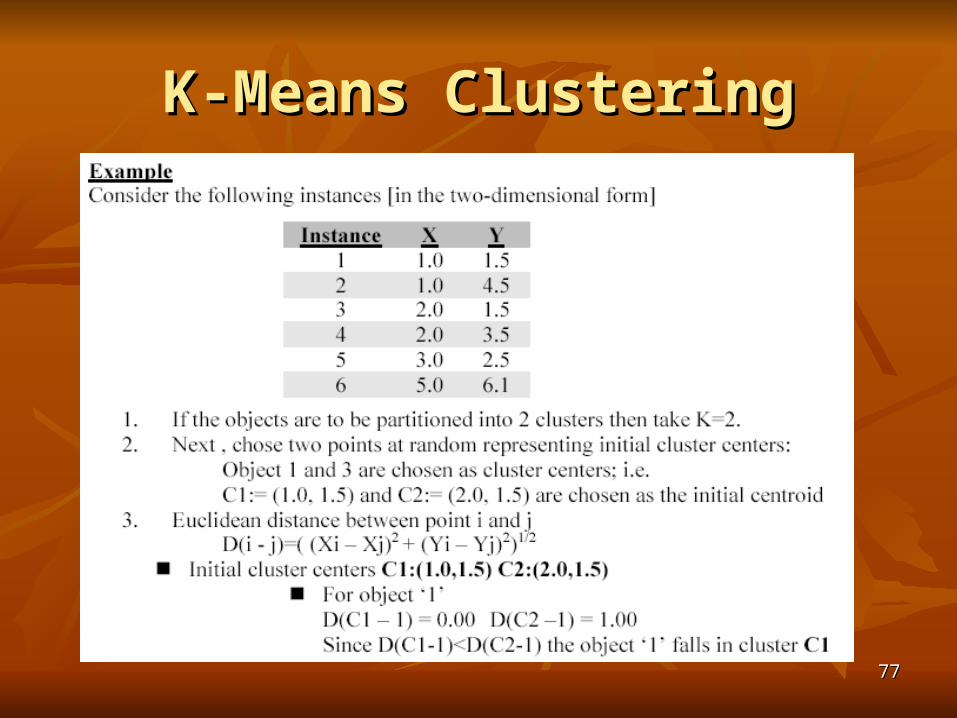
7777
K-Means ClusteringK-Means Clustering

7878
K-Means ClusteringK-Means Clustering

7979
K-Means ClusteringK-Means Clustering

8080
K-Means ClusteringK-Means Clustering

8181
Weakness of K-meansWeakness of K-means Applicable only when mean is defined, then
what about categorical data? Need to specify K, the number of clusters, in
advance run the algorithm with different K values
Unable to handle noisy data and outliers Works best when clusters are of approximately
of equal size

8282
Hierarchical ClusteringHierarchical Clustering
With hierarchal clustering, a nested set of cluster is created. Each level in the hierarchy has the separate set of clusters.
At the lowest level, each item is in its own unique cluster.
At the highest level, all items belong to the same cluster.

8383
Hierarchical Clustering: TypesHierarchical Clustering: Types AgglomerativeAgglomerative: :
starts with as many clusters as there are records, with each cluster having only one record. Then pairs of clusters are successively merged until the number of clusters reduces to k.
at each stage, the pair of clusters are merged which are nearest to each other. If the merging is continued, it terminates in the hierarchy of clusters which is built with just a single cluster containing all the records.
Divisive algorithm takes the opposite approach from the agglomerative techniques. These starts with all the records in one cluster, and then try to split that clusters into smaller pieces.

8484
AgglomerativeAgglomerative
DivisiveDivisive
Remove
Outlier
Remove
Outlier

8585
A Dendrogram Shows How the Clusters are Merged Hierarchically
Decompose data objects into a several levels of nested partitioning (tree of clusters), called a dendrogram.
A clustering of the data objects is obtained by cutting the dendrogram at the desired level, then each connected component forms a cluster.
A B C D E