Decision TreesDecision Trees

Review

• We introduced three styles of algorithms for linear classifiers:linear classifiers:– 1) Perceptron – learn classifier direction– 2) Logistic Regression – learn P(Y | X)) g g ( | )– 3) Linear Discriminant Analysis – learn P(X,Y)

• Linear separability– A data set is linearly separable if there exists a linear

hyperplane that separates positive examples fromhyperplane that separates positive examples fromnegative examples

Not linearly separable dataNot linearly separable data• Some data sets are not linearly separable!

O ti 1• Option 1– Use non-linear features, e.g., polynomial basis

functionsfunctions– Learn linear classifiers in the non-linear feature space– Will discuss more later

• Option 2– Use non-linear classifiers (decision trees, neural (

networks, nearest neighbors etc.)

Decision Tree for Playing TennisDecision Tree for Playing Tennis

Prediction is done by sending the example downPrediction is done by sending the example downthe tree till a class assignment is reached

DefinitionsDefinitions

• Internal nodes– Each test a feature – Branch according to feature values– Discrete features – branching is naturally definedg y– Continuous features – branching by comparing to a threshold

• Leaf nodesE h i l ifi ti– Each assign a classification

Decision Tree Decision Boundaries• Decision Trees divide the feature space into

axis-parallel rectangles and label each rectangle with one of the K classeswith one of the K classes

Hypothesis Space of Decision TreesHypothesis Space of Decision Trees• Decision trees provide a very popular and

ffi i t h th iefficient hypothesis space– Deal with both Discrete and Continuous features

– Variable size: as the # of nodes (or depth) of tree increases, the hypothesis space grows

• Depth 1 (“decision stump”) can represent any BooleanDepth 1 ( decision stump ) can represent any Booleanfunction of one feature

• Depth 2: Any Boolean function of two features and some Boolean functions involving three features:some Boolean functions involving three features:

• In general, can represent any Boolean functions

Decision Trees Can Represent Any B l F tiBoolean Function

XOR

• If a target Boolean function has n inputs, there always exists a decision tree representing that target function.H i th t ti ll d• However, in the worst case, exponentially many nodeswill be needed (why?)– 2n possible inputs to the functionp p– In the worst case, we need to use one leaf node to represent

each possible input

Learning Decision TreesLearning Decision Trees

• Goal: Find a decision tree h that achieves minimum misclassification errors on the training data

• A trivial solution: just create a decision tree with one path from root to leaf for each training example– Bug: Such a tree would just memorize the training data. It would

not generalize to new data pointsg p

• Solution 2: Find the smallest tree h that minimizes error– Bug: This is NP-HardBug: This is NP Hard

Top-down Induction of Decision TreesTrees

There are different ways to construct trees from data. We will focus on the top-down, greedy search approach:

Basic idea:1. Choose the best feature a* for the root of the tree.2. Separate training set S into subsets {S1, S2, .., Sk} where

each subset S contains examples having the same value foreach subset Si contains examples having the same value fora*.

3. Recursively apply the algorithm on each new subset y pp y guntil all examples have the same class label.

Choosing Feature Based on Classification ErrorClassification Error

• Perform 1-step look-ahead search and choose the attribute that gives the lowest error rate on the training datadata

0 10 1

0 1 0 1

U f t t l thi d t l k llUnfortunately, this measure does not always work well,because it does not detect cases where we are making “progress” toward a good tree

J=10J=10

J=10

Entropy• Let X be a random variable with the following probability distribution

P(X = 0) P(X = 1)

• The entropy of X, denoted H(X), is defined as

0.2 0.8

• Entropy measures the uncertainty of a random variable

���x

XX xPxPXH )(log)()( 2

py y

• The larger the entropy, the more uncertain we are about the value of X

If P(X 0) 0 ( 1) th i t i t b t th l f X• If P(X=0)=0 (or 1), there is no uncertainty about the value of X,entropy = 0

• If P(X=0)=P(X=1)=0.5, the uncertainty is maximized, entropy = 1

Entropy

• Entropy is a concave function downward

More About EntropyMore About Entropy• Joint EntropyJoint Entropy

C di i l E i d fi d�� ������x y

yYxXPyYxXPYXH ),(log),(),(

• Conditional Entropy is defined as)|()()|( xXYHxXPXYH

x����

– The average surprise of Y when we know the value of X

)|(log)|()( xXyYPxXyYPxXPx y

x������� � �

g p

• Entropy is additive)|()()( XYHXHYXH � )|()(),( XYHXHYXH ��

Mutual Information• The mutual information between two random variables X

and Y is defined as:

)|()()( XYHYHYXI– the amount of information we learn about Y by knowing the value

of X (and vice versa – it is symmetric).

)|()(),( XYHYHYXI ��

( y )

• Consider the class Y of each training example and the value of feature X1 to be random variables. The mutuala ue o ea u e 1 o be a do a ab es e u uainformation quantifies how much X1 tells us about Y.

X1P(X1=0)=0.6677 P(X1=1)=0.3333

H(Y|X1=0)=-0.6*log0.6-0.4*log0.4=0.9710

H(Y|X1=1)=-0.8*log0.8-0.2*log0.2=0.7219

H(Y|X1)=0.8879I(X1,Y)=0.0304

Choosing the Best FeatureChoosing the Best Feature• Choose the feature Xj that has the highest mutual

information with Y often referred to as the informationinformation with Y - often referred to as the informationgain criterion

)|(minarg

)|()(maxarg);(maxarg

jj

jj

jj

XYH

XYHYHYXI

�

��

• Define to be the expected remaining uncertainty

j

)(~ jJabout y after testing xj

)|()()|()(~ xXYHxXPXYHjJ jjj ���� � )|()()|()( xXYHxXPXYHjJ jx

jj �

Choosing the Best Feature: A General ViView

U(S)Benefit of split =

U(S)

PL PR

pU(S) – [PL*U(SL)+PR*U(SR)]

U(SL) U(SR)

Expected Remaining Uncertainty (Impurity)

Measures of Uncertainty

Error

Entropy

Gini Index

Multi-nomial FeaturesMulti nomial Features• Multiple discrete values

– Method 1: Construct multi-way split• Information Gain will tend to prefer multi-way split• To avoid this bias we rescale the information gain:• To avoid this bias, we rescale the information gain:

)|()(minarg

)|(minarg

xXYHxXPXYH jx

jj

���

��

– Method 2: Test for one value versus all of the

)(log)(minarg)(minarg

xXPxXPXH jx

jjjj ����

others– Method 3: Group the values into two disjoint

t d t t t i t th thsets and test one set against the other

Continuous Features• Test against a threshold• How to compute the best threshold � for X ?• How to compute the best threshold �j for Xj?

– Sort the examples according to Xj.M th th h ld � f th ll t t th– Move the threshold � from the smallest to thelargest valueSelect � that gives the best information gain– Select � that gives the best information gain

– Only need to compute information gain when class label changesclass label changes

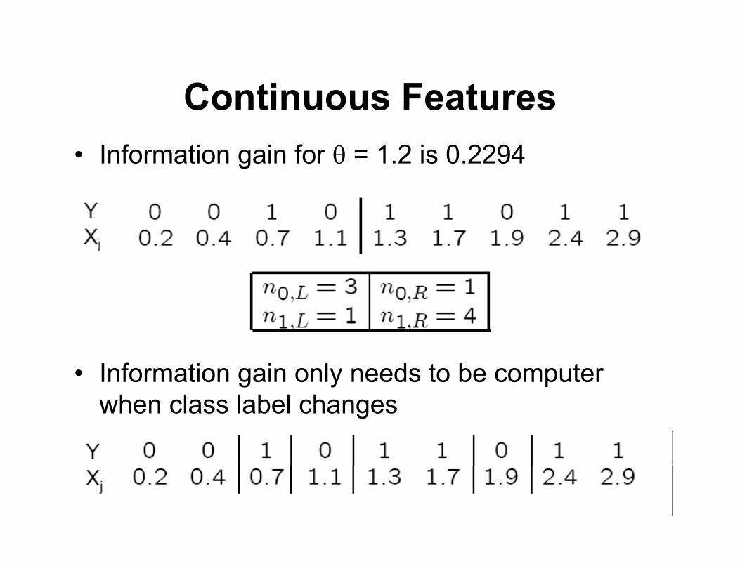
Continuous FeaturesContinuous Features• Information gain for � = 1.2 is 0.2294

n�;L � � n�;R � �n�;L � � n�;R � �n�;L � � n�;R � �

• Information gain only needs to be computer when class label changes

Top-down Induction of Decision TreesTrees

There are different ways to construct trees from data. We will focus on the top-down, greedy search approach:

Basic idea:1. Choose the best feature a* for the root of the tree.2. Separate training set S into subsets {S1, S2, .., Sk} where

each subset S contains examples having the same value foreach subset Si contains examples having the same value fora*.

3. Recursively apply the algorithm on each new subset y pp y guntil all examples have the same class label.

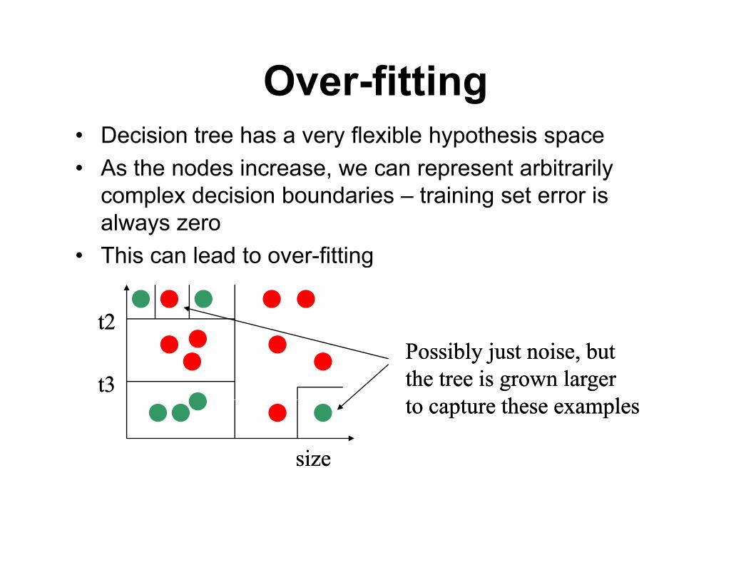
Over-fitting• Decision tree has a very flexible hypothesis space• As the nodes increase, we can represent arbitrarily

complex decision boundaries – training set error is always zero

• This can lead to over fitting• This can lead to over-fitting

t2t2t2t2

t3t3Possibly just noise, butPossibly just noise, butthe tree is grown largerthe tree is grown largert t th lt t th l

sizesize

to capture these examplesto capture these examples

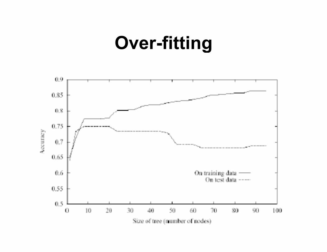
Over-fittingOver fitting

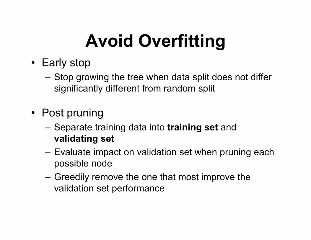
Avoid OverfittingAvoid Overfitting• Early stop

St i th t h d t lit d t diff– Stop growing the tree when data split does not differsignificantly different from random split

• Post pruning– Separate training data into training set and

lid ti tvalidating set– Evaluate impact on validation set when pruning each

possible nodepossible node– Greedily remove the one that most improve the

validation set performance

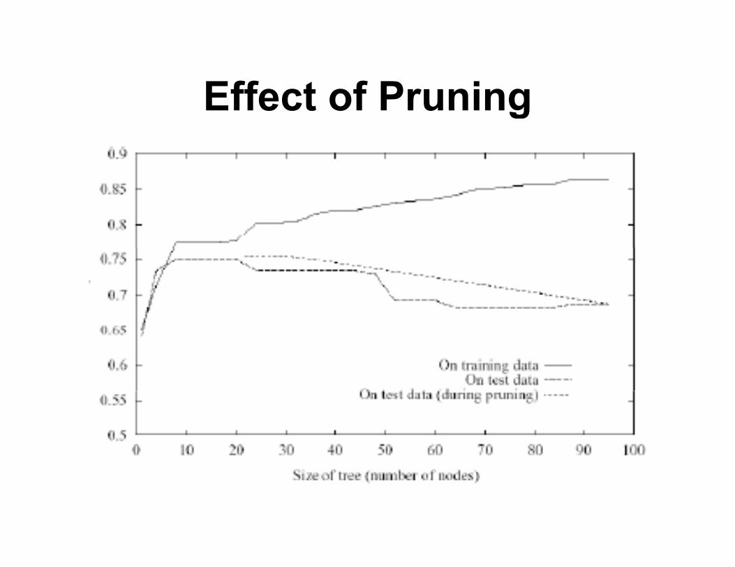
Effect of PruningEffect of Pruning

Decision Tree SummaryDecision Tree Summary• DT - one of the most popular machine learning tools

– Easy to understandy– Easy to implement– Easy to use

Computationally cheap– Computationally cheap

• Information gain to select features (ID3, C4.5 …)• DT over-fits

– Training error can always reach zero

• To avoid overfitting:– Early stopping– Pruning