impact of camex-4 data sets for hurricane forecasts … of camex-4 data sets for hurricane forecasts...
TRANSCRIPT

Impact of CAMEX-4 Data Sets for Hurricane Forecasts using a Global Model
Rupa Kamineni1, T.N. Krishnamurti1, S. Pattnaik1
Edward V. Browell2, Syed Ismail2 and Richard A. Ferrare2
1 Department of Meteorology, Florida State University, Tallahassee, Florida, 32306
2 NASA Langley Research Center, Hampton, Virginia, 23681
Submitted to: Journal of Atmospheric Sciences
for CAMEX-4 Special Section
Revised February 7, 2005
Corresponding Author Address:
Edward V. BrowellNASA Langley Research CenterHampton, Virginia 23681Email: [email protected]
https://ntrs.nasa.gov/search.jsp?R=20080014270 2018-05-26T13:52:31+00:00Z
2
Abstract
This study explores the impact on hurricane data assimilation and forecasts from the use
of dropsondes and remote-sensed moisture profiles from the airborne Lidar Atmospheric Sensing
Experiment (LASE) system. We show that the use of these additional data sets, above those
from the conventional world weather watch, has a positive impact on hurricane predictions. The
forecast tracks and intensity from the experiments show a marked improvement compared to the
control experiment where such data sets were excluded. A study of the moisture budget in these
hurricanes showed enhanced evaporation and precipitation over the storm area. This resulted in
these data sets making a large impact on the estimate of mass convergence and moisture fluxes,
which were much smaller in the control runs. Overall this study points to the importance of high
vertical resolution humidity data sets for improved model results. We note that the forecast
impact from the moisture profiling data sets for some of the storms is even larger than the impact
from the use of dropwindsonde based winds.

3
1. Introduction
A dominant factor for the improvement of weather forecasts is the quality and space-time
distribution of atmospheric measurements. The spatial distribution of in-situ atmospheric
measurements is highly inhomogeneous, largely being confined to Northern Hemisphere
continents, shipping routes at the surface, and a limited set of commercial airways confined to a
rather narrow range of altitudes and routes between major cities. Data-sparse regions include
much of the Tropics, the Southern Hemisphere, the Arctic, and much of the oceanic regions, at
least between the surface and commercial flight altitudes. The recent inclusion of space and
ground based remote sensing data compensates to some degree for the lack of in-situ
measurements. Satellite observations now cover the entire globe, and are relatively frequent in
time. Space-based remote sensing has the advantage of yielding relatively good coverage of
measurements with high temporal and horizontal resolutions.
Numerical weather prediction requires an accurate representation of the initial state of the
atmosphere. An error in the analysis of the initial state can amplify through the modeling
process and result in drastic errors in the predicted state. This is especially true in the case of
hurricanes and tropical storms. If the initial vortex is not well defined because of lack of data,
models may fail to predict the track and intensity of the storm.
Many field experiments (viz., STORM-FEST, FASTEX, WSR) have been conducted and
forthcoming experiments (viz., THORPEX) are to be carried out to enhance the database over
oceanic regions. The National Oceanic and Atmospheric Administration's (NOAA) Hurricane
Research Division (HRD) and its predecessors recognized that oceanic field experiments were
necessary back in the 1970’s, and they have been conducting annual field experiments in the
Atlantic and Pacific since even before that time. The Storm Scale Operational and Research
Meteorology Program Fronts Experiment Systems Test (STORM-FEST) field experiment was

4
conducted in the central United States between 1 February and 15 March 1992, and additional
soundings were taken along the west coast on several occasions to assess their effect on forecasts
downstream over the STORM-FEST area. This experiment was followed by the Front and
Atlantic Storm Track Experiment (FASTEX) (Thorpe and Shapiro, 1995), which involved major
operational forecast centers in an effort to improve operational numerical weather prediction.
Many different platforms were used to collect special data sets for testing various proposed
objective and subjective targeting strategies and for collecting data necessary for evaluating
forecasts over the open ocean. Later it was noticed that hurricane field experiments were
necessary over other oceanic regions adjacent to the United States; these regions are located off
the west coast, the Gulf of Mexico and the Caribbean Sea (Burpee et al., 1982; Simpson, 2003).
Recent sensitivity experiments on the observing network in the context of modern data
assimilation methods have indicated that the impact of data strongly depends on the location of
the data relative to dynamically sensitive parts of the flow. These sensitivity experiments
identify an important component to a successful sampling strategy, i.e., the identification of areas
in which initial condition errors are likely to amplify rapidly (owing to some dynamical
instability). Areas in which the initial condition errors are likely to be both large and rapidly
growing would be preferred areas to obtain supplementary observations. However, the recent
work by Aberson (2002, 2003) on hurricane targeting revealed that the way the targets are
sampled is the most important issue to be addressed. Studies by Graham (1990), Heming (1990),
Pailleux (1990), Rabier et al. (1996), Pu et al. (1997a) and Lord (1996) contain good examples of
definite positive impacts due to very few additional vertical profiles.
Sensitivity tests at the U.K. Meteorological Office (UKMO) (Graham and Anderson,
1995) and the National Centers for Environmental Prediction (NCEP) (Lord, 1993) have
demonstrated that improved wind observations have the greatest positive effect on one- to three-

5
day forecasts. Also, accurate dropsonde wind measurements in the vicinity of western Atlantic
and Caribbean hurricanes have markedly improved landfall predictions (Franklin and DeMaria,
1992). Certain specific forecast problems have been linked to lack of observations in most of the
regions. One example is hurricane track and intensity forecasting, which is one of the most
important forecast problems. Franklin and DeMaria (1992) and Burpee et al. (1996) showed that
dropwindsonde data collected by research aircraft demonstrably led to improved track forecasts,
which shows the importance of direct measurements in otherwise data-sparse regions.
Special reconnaissance aircraft operated by NOAA and by the U. S. Air Force continue to
provide valuable information for the prediction of hurricanes and severe winter storms.
Quantitative assessments of hurricane forecast improvements from including dropwindsonde
data from reconnaissance aircraft may be found in Burpee et al. (1996). Heming (1990)
discussed the impact of surface and radiosonde observations from two Atlantic ships on a storm
forecast. Smith and Benjamin (1993) demonstrated the benefits of wind data assimilation on
short-range forecasts in the eastern half of the United States. Recently Qu and Heming (2002)
discussed the impact of dropsonde data on forecasts of Hurricane Debby by the U.K.
meteorology office unified model.
The Convection and Moisture Experiment (CAMEX) consists of a series of field
experiments sponsored by the National Aeronautics and Space Administration (NASA). The
first two CAMEX field studies were conducted from Wallops Island, Virginia, during 1993 and
1995, and a third field study (CAMEX-3), which was specifically designed for hurricane studies,
was conducted from Patrick Air Force Base near Cocoa Beach, Florida, between 3 August to 28
September 1998. Recently, a fourth field campaign in the CAMEX series (CAMEX-4) was
conducted from 16 August to 24 September 2001 from a base at the Jacksonville Naval Air
Station, Florida. This field experiment was conducted in collaboration with the National

6
Oceanic and Atmospheric Administration's (NOAA) Hurricane Research Division (HRD) and
the United States Weather Research Program (USWRP). CAMEX-4 was focused on the study
of tropical cyclone (hurricane) development, tracking, intensification, and landfalling impacts
using NASA-funded aircraft and surface remote sensing instrumentation. One of the main
objectives of CAMEX is focused on studies of atmospheric water vapor and precipitation
processes using an array of airborne, space and land-based remote sensors. Our previous studies
showed promising impacts on hurricane forecasts using several CAMEX campaign data sets
(Bensman, 2000 and Rizvi et al., 2002). These studies provided the opportunity to address some
of the model failures in hurricane predictions.
In the present paper we have made an attempt to analyze the available CAMEX-4 data
sets using a three-dimensional variational analysis scheme (3DVAR). Medium range hurricane
predictions were carried out by integrating the NWP model out to 5 days with these new initial
conditions. This study was done using the FSU global spectral model. This paper is organized
as follows. Section 2 describes the CAMEX-4 data sets and the experimental plan using these
new data sets. Details of the analysis scheme and forecast model are provided in Section 3. The
numerical results are discussed in Section 4. Concluding remarks are provided in Section 5.
2. CAMEX-4 Data Sets
During CAMEX-3 and CAMEX-4, numerous observations were collected at various
stages of hurricane development. During the CAMEX-3 campaign, the observations were
targeted using an adaptive observational strategy based on a technique recently developed by
Zhang and Krishnamurti (1999). NASA's ER-2 and DC-8, NOAA’s Gulfstream-IV (G-IV) and
WP-3D, and the US Air Forces’s WC-130 weather reconnaissance aircraft were available during
this campaign.

7
a. Dropsonde
One of the NASA aircraft (DC-8) provided a high altitude research platform for a variety
of remote sensors, dropsondes and microphysical measurements in the inner core of the storm,
while another NASA aircraft, the ER-2, provided in situ data over the lower stratosphere, and
remotely sensed measurements through the troposphere. The flight altitude of the DC-8 was
generally from 30,000 to 40,000 ft and the ER-2 was at nearly 65,000 ft. Two NOAA P-3s were
used for both hurricane research and reconnaissance. The P-3s penetrated the eyewall repeatedly
at altitudes from 1,500 to 20,000 ft. The NOAA G-IV was used to derive a detailed picture of
the upper atmosphere surrounding the hurricanes as well as to provide dropwindsonde
measurements. It provided measurements of the upper level hurricane steering winds that are
important for determining the track of a hurricane. The G-IV flew between 350 and 1500 km
from the eye of the hurricane and at altitudes up to 45,000 ft. The US Air Force's WC-130
reported hurricane conditions through a combination of visual observations and onboard in situ
instruments. Our data assimilation includes these data sets at about 3-minute intervals. The
assignment of error for this analysis assumes that these measurements are of the same quality as
data sets from commercial aircraft. Further details of these instruments can be found on the
CAMEX-4 website (http://camex.msfc.nasa.gov).
This mission was designed to collect, process and transmit analyses of vertical
atmospheric soundings in the environment of a hurricane. Dropsondes provide invaluable
information about winds in the mid-level hurricane vortex and also the vertical temperature
distribution within the eye. The dropsonde system uses Global Positioning System (GPS)
dropwindsondes to measure vertical profiles of pressure, temperature, humidity and wind during
descent to the surface. These data were measured every 0.5 s (2 Hz) during the descent. The
Airborne Vertical Atmospheric Profiling System (AVAPS) was used for monitoring the
8
dropsondes from the operational and research aircraft. Additional information on the GPS
dropwindsondes can be found in Hock and Franklin [1999]. During this campaign, up to 150
dropsondes were deployed from both the NASA DC-8 and ER-2, and nearly 70 of those were
dropped on the last three days of the experiment.
Figure 1 shows the sample dropsonde data coverage at various levels from multiple
aircraft on 23 September 2001 in conjunction with study of Hurricane Humberto. The bottom
panel of Fig. 1 shows the coverage at lower levels (850 hPa); the middle panel shows the
coverage at middle levels (500 hPa); and the top panel shows the upper level (200 hPa) coverage.
On this day, the G-IV aircraft covered the large-scale environment of the hurricane and the other
aircraft covered the eye and inner region. The upper level data were provided by the DC-8, ER-2
and G-IV. The low level cyclonic and the upper level anticyclonic patterns can be clearly seen in
the wind data. This intensive data coverage was a highlight of the CAMEX experiments.
b. LASE (Lidar Atmospheric Sensing Experiment)
The LASE instrument was developed at the NASA Langley Research Center as the first
autonomously operating Differential Absorption Lidar (DIAL) system, and it was initially flown
on the NASA ER-2 aircraft for profiling water vapor, aerosols and clouds through the entire
troposphere (Browell et al., 1995, 1997; Moore et al., 1997). The accuracy of the LASE water
vapor profile measurements was first demonstrated in the 1995 LASE Validation Experiment
where comparisons of the LASE water vapor measurements with in situ water vapor
measurements on two additional aircraft (C-130 and Lear Jet), radiosonde profiles, and profiles
from a ground-based Raman lidar showed agreement to be better than 6% or 0.01 g/kg,
whichever is greater throughout the troposphere (Browell et al., 1997). Subsequently LASE was
flown on the ER-2 during the Tropospheric Aerosol Radiative Forcing Observation Experiment
(Ismail et al., 2000; Ferrare et al., 2000a,b) and in seven other major field experiments onboard

9
the NASA P-3 and DC-8 aircraft. Intercomparisons performed during the CAMEX-3 (Ferrare et
al., 1999; Browell et al., 2000), Pacific Exploratory Mission (PEM) Tropics B (Browell et al.,
2001), and CAMEX-4 (Kooi et al., 2002) missions produced results consistent with the initial
LASE validation experiments.
The impact of including LASE data in the hurricane analysis compared to the ECMWF
(European Centre for Medium-Range Weather Forecasts) analysis without LASE data was
recently described by Kamineni et al. (2003). The result of combining the LASE and dropsonde
data in hurricane analysis is described in this study.
c. Design of Experiments
A special dataset on 0.5 degree latitude by 0.5 degree longitude at 28 vertical levels
without inclusion of dropwindsonde data has been provided to us by ECMWF. We have used
these data in our analysis. This analysis also included operational global sets from the stream of
the world weather watch, cloud track winds, commercial aircraft winds reports, surface data sets
from marine ships of opportunity, oceanic buoy surface reports, ocean surface winds from
satellite based scatterometers, sounding of temperature and humidity from polar orbiting
satellites. The microwave radiances provided by TRMM (Tropical rainfall Measuring Mission)
and DMSP (Defense Meteorological Satellite Program) satellites (F13, F14 and F15) provide
rain rate estimates via NASA Goddard algorithms (Olson et al. 1990). The Florida State
University (FSU) model at a T126 resolution makes use of these data to perform a physical
initialization (Krishnamurti et al., 1991). The T126 resolution of the FSU model was noted to be
adequate for exploring the extent to which the larger scale hurricane was resolved by the aircraft
data sets. Our definition of a first control (CTRL) forecasts includes the ECMWF plus rain rate
estimates in its initial state at the T126 resolution. Subsequent to that we generated another
control run (CTRL1), where all the available winds (flight level plus dropsonde winds) using

10
CTRL as background were assimilated. This is the NEW control run which is now being used as
background field for all other experiments. Here we have used both the dropsonde and the flight
level data, since our aim is to utilize more and more wind information to define the hurricane
structure. However, the experiments were designed mainly to focus on the impact of water
vapor measurements (either dropsonde or LASE), which is a goal of our study. The objective of
this analysis is to forecast the broad scale evolution of hurricanes.
Dropwindsonde data from the six aircraft (two NOAA P-3's, US Air Force C-130, NASA
ER-2 and DC-8, and NOAA G-IV), flight level in situ data from the DC-8 and P-3 aircraft, and
LASE water vapor profiles collected from the DC-8 aircraft were used in the following
experiments:
CTRL: Control analysis at T126L14 (Triangularly truncated at 126 wave in horizontal and 14
sigma levels in vertical) by using ECMWF analysis at 0.5-deg resolution + FSU Physical
Initialization.
CTRL1: CTRL + all the available wind data during CAMEX-4. It served as background field
for the following experiments.
EXP1: CTRL1 + dropsonde moisture data sets
EXP2: CTRL1 + LASE data sets
EXP3: CTRL1 + dropsonde moisture + LASE data sets. This includes all of the available data
sets.
3. Data Assimilation
A typical data assimilation system is composed of a forecast model that provides a
background, first guess of the atmosphere by extrapolating information forward from previous
observations, and an analysis that combines information from the background and from the entire

11
set of widely scattered observations into a model-compatible form for extrapolation to the next
analysis time. Since data assimilation has observational, analysis and the modeling components,
improvements in one or more of these components are expected to improve forecasts.
a. Analysis scheme
Analysis is a process by which various meteorological observations distributed in space
and time from different observing systems are integrated with other information, like short range
weather predictions (6 hours) from a NWP model, previous analysis, climatology etc., to form a
numerical representation of the initial atmospheric state. CAMEX-4 data were analyzed using a
three-dimensional variational analysis scheme which is mainly based on Lorenc’s (1986) concept
of minimizing a generalized cost function using the Spectral Statistical Interpolation (SSI)
technique (Parrish & Derber 1992). The cost function used in this scheme is as follows.
J(X) = 1/2 [ (X-Xb)T B-1(X-Xb) + (Yobs-H(X))T R-1 (Yobs-H(X)) ] (1)
Where, X = N-component vector of analysis variables; Xb = N-component vector of first guess
variables; Yobs = M-component vector of observations; B = N x N background error co-variance
matrix; R = M x M observational error co-variance matrix; H = an operator from analysis to
observation space (possibly non-linear); N = analysis degree of freedom; M = number of
observations; and ( )T = transpose of the matrix.
The two terms in J on the right hand side of Eq. (1) deal with the fit of the first guess field
and the observations with the desired analysis, respectively. In order that the analysis should fit
best with both the first guess and the observations, J should be minimized with respect to the
analysis variable X. The minimization is accomplished by using a standard conjugate gradient
(CG) (Chandra, 1978) descent algorithm, which allows R to be non-linear.
Let us define a variable W as: W = C-1(X-Xb) (2)
The matrix C, is related to the forecast errors and is given by B = C CT (3)

12
Minimization of J leads to the following analysis equation: Aδ = f (4)
Where L ( = ∂H/∂X ) is the tangent linear operator of the operator H; A = [ I + CT LT R-1 L C ];
and f = CT LT R-1 [ Yobs - H( Xb + C W) ] - W.
Using a perturbation technique, the solution of the analysis equation (4) is obtained for
W., Finally the state vector X, which minimizes J, is determined using (2) and (3). The
following iterative algorithm is used for solving the analysis equation.
Set X = Xb , W = 0
Do k = 1,n outer (Outer iteration)
evaluate f = CT LT R-1 [ Yobs - H( Xb + C W)] - W
solve Aδ = f using an iterative conjugate gradient algorithm (5)
W = W + δ
X = X + C δ
End do
Here one important thing to be noted is that the tangent linear operator is always
evaluated with the latest X and the non-linearity in H, which results from the dependence of the
sigma co-ordinates on the surface pressure, is not included in L. However, each time the vector f
is evaluated, a complete H-operator is utilized.
Further details about the choice of the analysis variables, balance between the mass and
the wind field, vertical coupling, the statistical parameters used, etc., are given in Parrish and
Derber (1992), and Rizvi and Parrish (1995). The statistical parameters, like the background
error covariance, Empirical Orthogonal Functions (EOF) for vorticity, divergence, temperature,
moisture and various other statistical parameters defining the partitioning between the fast and
the slow part of the flow, are computed using the difference between the day-1 forecasts and the
corresponding verifying analysis for that date. A 40-day data set (August - September 1998) was

13
used to compute these statistics. The amplitudes and scales of the background errors have to be
tuned to represent the (6-hr, 3-hr) forecast errors in the guess field. This is the reason for the
tuning parameters mentioned above. The statistics that project multivariate relations among
variable are also derived from the NCEP method.
b. Forecast model
The global model used in this study is identical in all respects to that used in
Krishnamurti et al. (1991). This comprehensive model carries the spectral transform method
with the semi-implicit time differencing scheme for the dynamics. An array of physical
parameterization schemes are used for shallow and deep cumulus convection, dry convective
adjustment, radiative transfer based on a band model for short and long wave radiances, surface
fluxes, surface energy balance, definition of clouds for radiative transfer, and the use of the
sigma coordinate surface for the treatment of orography. The relevant references on these model
components are provided in Krishnamurti et al. (1991). The current horizontal resolution for the
CAMEX studies is T126 and in vertical we use 14 layers. In addition to these features the model
includes a physical initialization component based on Krishnamurti et al. (1991, 2001). The
sequence of steps in our modeling starts with a special operational level-three analyzed data set
from the ECMWF. This data set is received at FSU at a resolution of 0.5° latitude/0.5° longitude
at 28 vertical levels. These data are interpolated to the FSU transform grid at the resolution
T126. At this stage precipitation estimates based on microwave radiance data sets from TRMM-
TMI (TRMM Microwave Imager) and DMSP-SSM/I (Special Sensor Microwave/Imager)
satellites are used for the physical initialization that provides a nowcasting of the initial rain rate
for the model. The proposed data assimilation that incorporates the additional data sets from the
CAMEX-4 research aircraft (dropwindsonde, LASE and flight level) follows sequentially after
the completion of physical initialization. The SST analysis for this modeling was obtained from

14
NOAA/NESDIS operational real time analysis files that were based on weekly averages
(preceding the initial state for each storm) and included datasets from surface ships, buoys and
satellite derived estimates.
Several techniques have been developed to assess the influence of new data sets for the
analysis/forecast issues. In this study, the data-denial experiment (DDE) procedure was used to
assess the impact of new data sets on hurricane analysis and forecasts. In this technique actual
forecast/data assimilation cycles are re-run, selectively excluding actual observations, and the
relative degradation or improvement noted. By examining many such cases, the effect of the
exclusion of certain data sets can be assessed.
4. Numerical Results & Discussion
The outputs of the various experiments that were analyzed and the impacts on the
hurricane forecasts are discussed in the following subsections.
a. Impact on hurricane track and intensity
In our sensitivity analysis of the forecasts to the assimilation of CAMEX-4 data sets, we
primarily focused on some representative fields such as the mean sea level (MSL) pressure.
Comparisons with the verifying ECMWF analysis and officially-issued best track from the
National Hurricane Center (NHC) were also made. The various forecast tracks for Hurricanes
Erin, Humberto and Gabrielle are presented in Fig. 2 (a, b and c). The legend in these figures
distinguishes between the different model runs for each storm. Since the research aircraft flights
were limited, generally only one complete set of experiments was possible for each of these
storms. Although there were two complete missions flown for Humberto, only one data set is
used here. For Erin and Gabrielle, the forecast track for the control run was generally in the
approximate heading of the storms, moving northeastward, but was behind the actual storm
position due to the erroneously slow translation speed. On the other hand, forecast tracks with

15
CAMEX-4 data sets were almost parallel to each other and followed the best track closely.
However, the initial storm positions in the control and the experiments were very close to the
best track position. In the case of Humberto, the forecast track of the control run showed the
tendency of recurvature; however, the slow forecast speed increased the distance error
substantially reaching 340 km at 72 hours forecast. Assimilation of the maximum amount of
available data (EXP3) resulted in the smallest distance errors of 120 and 150 km at 72- and 96-
hour forecasts, respectively.
Overall we note that, in general, there is a sequential improvement in track forecasts as
more and more data sets were added. The best track forecasts, in general, were found when the
flight level data, the dropsonde data (wind, and humidity) and the LASE moisture profiles were
all incorporated within the data assimilation. These data sets were added to those of the control
run which only included the ECMWF analysis. The addition of moisture data from all the
distributed dropsondes improved the forecast errors well beyond what was possible from LASE
data alone. This is due to the much larger coverage of moisture profiles from the 100 or so
dropsondes from six aircraft. LASE provided moisture profiles from one aircraft (DC-8) and
mainly in cloud free areas.
These results for Hurricanes Erin and Gabrielle essentially demonstrated that as more and
more data were introduced (beyond those of the control experiment) the left bias of the control
experiments was generally reduced with the addition of each new data set. This left bias is
largely related to the positive surface vorticity tendency that arises from the larger scale
horizontal advection of vorticity in the lower troposphere. This feature is similar for all of the
above experiments and occurs downwind from the wind maximum of the hurricane. As
dropsonde and LASE data sets were sequentially introduced, the hurricane was better resolved
on a smaller scale. The model showed a pronounced center of rising motion, precipitation and

16
positive vorticity tendency where this storm was now being resolved. This occurred to the right
of the track of the control run, and the control run’s track appeared to be mostly dictated by the
larger scale vorticity advection. The local enhancement of the diabatic processes appears to
display a positive tendency for the precipitation enhancement from the storm’s newer data sets.
It is easy to see how that pushes the positive vorticity maxima to the east of the control
experiment. In a related study, Krishnamurti et al (1997) noted that if several different initial
analyses were deployed within the same model, then either a left or a right bias developed in the
forecasts depending on which initial analysis was used within the same model. This appears to
be related to differences in the initial vorticity advection downwind of the velocity maxima of a
hurricane, which was located at different places for various analysis used in that study. This
suggests that a left or a right bias could be reduced somewhat simply from the enhancement of
the initial data sets or from ensemble forecasts that use several initial analyses.
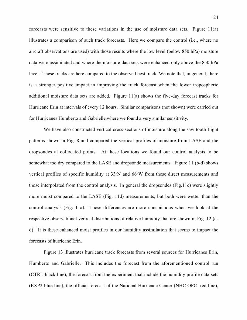
The MSL pressure of all the three storms was examined for all the experiments. The
forecast intensities of the minimum MSL pressure from all the experiments were 4-8 hPa lower
than those in the control run. Figure 3 shows the MSL pressure on day 3 of forecasts for
Humberto for the various experiments. The pressure forecasts for the same sequence of
experiments (Analysis, CTRL, CTRL1, EXP1, EXP2, and EXP3), as shown in Fig. 3, are 990,
998, 996, 994, 996 and 990 mb, respectively. The minimum MSL pressure estimated by NHC
was 992 mb. Nearly the same differences were found for Erin and Gabrielle (not shown).
Figure 4 shows track errors for these hurricanes. In the case of Humberto and Erin, the initial
errors were small, and these errors were further reduced in the experiments. In case of Gabrielle
the initial large errors were amplified during model integration; however, these errors were
reduced in the experiments. Overall these errors were reduced significantly up to day-3
forecasts. A combination of LASE plus the dropsonde data provided the best result.

17
Furthermore, the results from EXP1 were better than those of EXP2. The possible reason is that
the dropsondes from different aircraft provided coverage over many different locations over and
around the hurricane. However, all the experiments had improved forecast tracks with stronger
intensity and faster movement in comparison with the control run.
The intensity forecast errors for the maximum storm winds for Erin, Humberto and
Gabrielle are shown in Fig. 5. The wind speed errors are shown in knots at the 850 hPa level.
Here we compared the relative error for the two control runs with those of the dropsonde, LASE
and combined observation based experiments. The best results in all cases came from the use of
all humidity data sets (dropsonde plus LASE, i.e., EXP3). These show a major improvement
over the control results where none of the CAMEX data sets were used. The major message of
Fig. 5 is that there is a positive impact on hurricane intensity from the inclusion of improved
humidity data sets.
Given the wind forecasts on a latitude/longitude grid, it is possible to use coordinate
transformation to cast data sets in polar co-ordinates with respect to the storm center, i.e., in
storm relative coordinates. This is an objective algorithm that facilitates the examination of a
storm’s intensity after an azimuthal averaging is performed. This was done for day 3 of the
forecasts derived from the control run (CTRL), CTRL1, EXP3 and for the validated analysis.
In Fig. 6 we show the results for the tangential wind. The abscissa is the radial distance
from the storm center in km and the ordinate shows the azimuthally averaged tangential velocity
at the 850 hPa level. The legend identifies these different data sets. The crosses show the results
for the experiment that carries the most data sets. The three panels show results for the different
storms Erin, Gabrielle and Humberto. Overall we note that the intensity forecasts do show some
improvement as we add more and more data sets. What is most interesting here is that there is
marked improvement in the intensity forecast as we proceed from CTRL1 to EXP3. This simply
18
means that the addition of humidity data from both the dropsonde and LASE had a significant
positive impact on the intensity forecasts over and above what was possible from the addition of
winds from dropwindsonde and the flight level measurements. A surprising lack of
improvement in the inner radii (< 200 km) for Gabrielle may be related to the lack of the
effectiveness of humidity measurements in rain areas.
b. Impact of extended moisture data coverage on hurricane forecasts
In storm relative co-ordinates the moisture transport vector qV has an interesting
structure. We have vertically averaged this vector over 200-1000 hPa to examine the moisture
transports for Erin at 12UTC on 10 September 2001. This is displayed in Fig. 7 as streamlines of
qV . One of the major moist swaths (red) of air enters the storm from the south, whereas a dry
air swath (yellow) is seen to spiral in from the north. The LASE data were provided by the DC-8
aircraft flights over a portion of the storm where, in storm relative coordinates, a moist band of
air enters the storm. The motivation for displaying structure was to see the active quadrants of
the storm where moisture enters the hurricane center. The ranger markers are arbitrarily marked
at every 30 degrees and the radial distance from center to outer radii is 370 km. The flight track
along this moist band was designated as an “optimal data assimilation flight plan,” and this type
of flight plan was used during the CAMEX-3 (Danielle) and CAMEX-4 (Erin) campaigns. The
goal of this flight plan was to assess the impacts of high-resolution water vapor and wind
measurements on the forecasts of hurricane intensity and tracks.
Figure 8 illustrates the aircraft flight track of the DC-8 during a moisture transport
mission for studying Hurricane Erin during CAMEX-4. A similar mission was also flown for
Hurricane Danielle during CAMEX-3. These tracks were specifically designed to provide
moisture data sets to the south of the hurricane (over relatively clear sky areas). The design of
this mission was specifically aimed at obtaining a detailed description of the moisture transports

19
)( qVn at two different radii from the storm center. This moisture transport was provided by the
dropwindsonde data from the DC-8 and LASE profiles of moisture. Two versions of data
assimilation, with and without the LASE data, were used to estimate these humidity transports.
We also examine the differences between the LASE-based transports and those of the control
experiment which did not include the LASE data sets. For this purpose we determined the
vertical cross-sections proceeding from west to east following the outer and inner segments of
the flight tracks that are shown in Figs. 9.1 and 9.2. In this case, dropwindsondes provided the
vertical profiles of winds and LASE provided the vertical profiles of specific humidity. Figure
9.1 displays the results based on Hurricane Erin’s analysis (Fig. 9.1 a, b, c and d) and 72-hour
forecasts (Fig. 9.1 e, f, g and h), respectively. The left panels (Fig. 9.1 a, b, e and f) show the
results for the inner segment of data, and the right panels (Fig. 9.1 c, d, g and h) show the results
for the outer segment. We see here that the moisture transports that included the LASE data
were invariably larger (Fig. 9.1 a and b) than those of the control (Fig. 9.1 c and d) where LASE
data were excluded. The moisture transport in the inner segment was found to be conspicuously
larger than the transport in the outer segment. This suggests a divergence of moisture flux
between the outer and inner segments. The resulting strong evaporation in the storm’s vicinity
may have been a factor in producing the stronger intensity of Erin which had reached a category-
3 level.
The corresponding results for Hurricane Danielle in 1998, where similar flights of the
NASA DC-8 were flown, are shown in Fig. 9.2. This shows Danielle’s analysis (Fig. 9.2 a, b, c
and d) and 72-hours forecasts (Fig. 9.2 e, f, g and h), respectively. The left panels (Fig. 9.2 a, b,
e and f) show the results for the inner segment of data, and the right panels (Fig. 9.2 c, d, g and
h) show them for the outer segment. Here we found a similar structure in the analysis (i.e., day-
0) for the moisture transports, although the magnitudes were considerably less. Hurricane

20
Danielle was a category-1 storm, and it did not exhibit as much mass and moisture convergence
as were seen for Hurricane Erin. The convergences were further reduced when the forecasts for
Danielle were examined. The inner and outer moisture transport was nearly equal. In the case of
Danielle, the convection became more tightly wrapped around the center and the moisture
convergence was closer to the center. Furthermore, the selection of the date and the flights flown
around these hurricanes may have been another factor since the storms were going through a life
cycle of amplification or decay at these observational times. The time series of the intensity
shows that Erin was slightly weakening whereas Danielle was in a decaying stage. Thus, large
impacts of these new data sets were noted in the magnitude of the moisture flux convergences
that were missed in the control run.
c. Moisture Budget
We shall next discuss the moisture budget of these storms, where the moisture transports
appear to have a critical role in the overall hurricane behavior. Basically the water vapor budget
contains elements such as: Storage = convergence of flux of moisture + evaporation
–precipitation. These are integrals over a mass of the atmosphere where,
( ) ( ) dprdrdg
dmwherer
r
p
pm
θθ∫∫∫∫ =2
1
2
1
1 (6)
and these mass elements are enclosed inside circles of radii r1, and r2, around the hurricane from
the top of the atmosphere p = p1 to the earth’s surface where the pressure is p = p2.
The three storms Erin, Gabrielle and Humberto were in different stages of their life cycle.
1) Erin: On 10 September 2001 at 1200 UTC, Hurricane Erin’s minimum pressure was 969 hPa
and maximum wind was around 100 kts. In the following 24 hours the minimum pressure rose
to 976 hPa and the maximum winds dropped to 80 kts.

21
2) Gabrielle: On 15 September 2001 at 1200 UTC, the central pressure of Gabrielle (a tropical
storm at this stage) had a minimum pressure of 998 hPa and an intensity of 40 kts. In the
following 36 hours the central pressure dropped to 991 hPa and the maximum winds reached
hurricane strength of 65 kts.
3) Humberto: On 22 September 2001 at 1200UTC, the central pressure of the tropical storm was
1007 hPa and maximum wind of 40 kts. In the next 24 hours the central pressure dropped to 990
hPa and the maximum winds reached hurricane strength of 65 kts.
Given the assimilated data sets and the day-3 forecasts for Hurricane Erin, Gabrielle and
Humberto it was possible to evaluate these terms for all of the experiments carried out in this
study. Using storm relative coordinates, and a local cylindrical frame of reference about the
storm center, the moisture budget is expressed by the following relations:
Moisture Continuity Equation:
rrqV
rrqV
qVWhere
PEvapdmpq
Vdmqdmtq
r
mmm
∂∂
+∂
∂=∇
−+∂∂
−∇−=∂∂
∫∫∫
1.
,.
θ
ω
θ
(7)
The budget was estimated from various data sets generated by our model (i) Control data
sets (CTRL), (ii) experiment that includes LASE data sets (EXP2) and (iii) experiment that
includes dropsonde and LASE data sets (EXP3). These data sets are all derived using the
3DVAR data assimilation. Figure 10 (a to f) shows these budgets for Hurricanes Erin, Gabrielle,
and Humberto in storm relative coordinates for these three data sets. These budget diagrams
carry the following information: (i) Local change )/( tq ∂∂ , i.e., source or sink, (ii) convergence
of flux (positive sign), (iii) precipitation (P) and (iv) evaporation (Evap). These are all quantities

22
provided by the model at time 0 and at 72-hour forecasts. The following is the summary of
moisture budget for these individual storms.
i) Erin: (Fig. 10 a & b). The initial evaporation at a radial distance of 200 to 300 km from
storm center increased from 206 to 353 to 503 mm/day as we proceed from the control (CTRL)
to LASE (EXP2) and to the final experiment with all data sets (EXP3). There was in fact a spin
down of evaporation by day 3 of the forecast at these radii to values of 160, 218 and 298
mm/day, respectively. This is consistent with the observation that Hurricane Erin was
weakening somewhat. This spin down of evaporation was also evident at an outer radii near
1000 km. Unlike the evaporation, the precipitation amount did not show a significant decrease
in intensity with the spin down. In general, larger rainfall rates were found for the experiments
that included more and more humidity data sets in their initial analysis. With the weakening of
Erin we also found spin down of the net convergence of moisture flux. It is possible that an
increase in evaporation rate and storm intensification are concurrent indicators, and as such, it
may not necessarily imply causality.
ii) Gabrielle: (Fig. 10 c & d) Gabrielle was an intensifying storm in these cases.
Between 200- and 300-km radii at the initial time the evaporation increased sequentially from
222 to 363 to 608 mm/day as we proceed from the control to LASE to the final full data
experiment. The local change )/( tq ∂∂ , i.e., source or sink, convergence of flux, precipitation
and evaporation, of the moisture budget was extremely large at the initial time, perhaps
contributing to initial intensification of Gabrielle from a tropical storm to a hurricane. Therefore,
the moisture budget reveals an equilibration toward somewhat lower values.
iii) Humberto: Figure 10 e & f displays the moisture budgets for Hurricane Humberto.
Here we can see for the day 0 an increase in the convergence of fluxes from 51 to 160 to 245
between 200 and 300 km from the storm center. The forecasts seem to retain some of these
23
impacts even at day 3. The differences between LASE based and LASE plus dropsonde based
forecasts are, however, not as large at 72 hours as they were at hour zero. However, they do
have much larger values compared to the control at 72 hours.
In general, for day-0 fields we find a gradual increase in the convergence of fluxes of
moisture as we proceed from the control data-based experiment to LASE data-based experiment
and on to the all inclusive data-based experiments. It is very clear that as the convergence of
moisture flux increases so does evaporation and precipitation within the radial legs (around the
storm). Although the detailed precipitation fields are not shown here, in the inner radii inside r <
500 km the satellite pictures clearly confirm higher rainfall in those inner belts.
This clearly shows the impact of including the additional moisture data from LASE and the
dropsondes as well. The control analysis that only includes the moisture analysis from the world
weather watch underestimates the precipitation compared to the observed estimates of rain
amounts.
The moisture budgets at 72 hours show increased values for the transports and divergence
of flux of moisture as we sequentially compare results of experiments with added data sets,
(especially moisture data sets). Furthermore, the impacts from the added moisture data sets are
quite robust. The precipitation forecasts in excess of 120 mm/day along those radial legs from
the LASE and LASE plus dropsonde experiment are in line with the observed estimates. The
precipitation rates were underestimated by the control run. This shows that forecasts that include
moisture profile data sets can contribute to a positive impact. Since the moist processes are most
important for a hurricane, such profiling data sets of humidity may be important for the modeling
of the heavy rain areas.
We have also explored the sensitivity of track forecasts to the use of enhanced moisture
profiling observations in the lower versus the upper troposphere. We noted that the track
24
forecasts were sensitive to these variations in the use of moisture data sets. Figure 11(a)
illustrates a comparison of such track forecasts. Here we compare the control (i.e., where no
aircraft observations are used) with those results where the low level (below 850 hPa) moisture
data were assimilated and where the moisture data sets were enhanced only above the 850 hPa
level. These tracks are here compared to the observed best track. We note that, in general, there
is a stronger positive impact in improving the track forecast when the lower tropospheric
additional moisture data sets are added. Figure 11(a) shows the five-day forecast tracks for
Hurricane Erin at intervals of every 12 hours. Similar comparisons (not shown) were carried out
for Hurricanes Humberto and Gabrielle where we found a very similar sensitivity.
We have also constructed vertical cross-sections of moisture along the saw tooth flight
patterns shown in Fig. 8 and compared the vertical profiles of moisture from LASE and the
dropsondes at collocated points. At these locations we found our control analysis to be
somewhat too dry compared to the LASE and dropsonde measurements. Figure 11 (b-d) shows
vertical profiles of specific humidity at 33oN and 66oW from these direct measurements and
those interpolated from the control analysis. In general the dropsondes (Fig.11c) were slightly
more moist compared to the LASE (Fig. 11d) measurements, but both were wetter than the
control analysis (Fig. 11a). These differences are more conspicuous when we look at the
respective observational vertical distributions of relative humidity that are shown in Fig. 12 (a-
d). It is these enhanced moist profiles in our humidity assimilation that seems to impact the
forecasts of hurricane Erin.
Figure 13 illustrates hurricane track forecasts from several sources for Hurricanes Erin,
Humberto and Gabrielle. This includes the forecast from the aforementioned control run
(CTRL-black line), the forecast from the experiment that include the humidity profile data sets
(EXP2-blue line), the official forecast of the National Hurricane Center (NHC OFC -red line),
25
and a forecast based on the FSU superensemble (SUPENS-purple line). Also shown are the
observed best track positions (green line). We found in all cases that the experiments that
included the humidity profile data sets perform better than the control and at times were better
than the official forecasts. The FSU superensemble has the best performance since it assimilates
the results from several models (Williford et al., 2003).
The current experiments on Erin, Gabrielle and Humberto using LASE and
dropwindsonde data were not part of the real-time forecasting effort. It is interesting to note that
only for Erin did the operational superensemble perform better than these new experiments. For
the other two storms, Gabrielle and Humberto our forecasts with the LASE and dropwindsonde
moisture data appear to have done very well in comparison to the operational forecasts. This
suggests that the use of humidity profile data in single forecasts can perhaps provide a useful
member for the superensemble. Such a direct test is not possible, since the superensemble
requires a training database of as many as 60 forecasts from each member model, and the LASE
and dropwindsonde data were not available for such a series of past forecasts.
5. Conclusions
This study explores the impact of additional data sets beyond those that are currently
available for operational weather prediction. The conventional data sets include surface and
radiosondes, ships of opportunity, oceanic buoys, commercial aircraft platforms, cloud and water
vapor tracked winds and satellite based soundings. Those were analyzed via the four-
dimensional data assimilation by the European Center for Medium Range Weather Forecasts,
which were provided to us. The goal of this study was to examine the impact of dropwindsonde
(profiles of winds, and humidity) and/or LASE (moisture profiles) data sets during CAMEX-4 on
hurricane analysis and forecasting. These new observations, especially the winds from the
dropsondes and aircraft flight levels and moisture profiles from the dropsondes and LASE, were
26
analyzed sequentially using 3DVAR, and medium range predictions were then carried out by
integrating the FSU global spectral NWP model out to 5 days with these new initial conditions.
The forecast of tracks and intensity from the assimilation experiments demonstrate
improvement over control experiments. The inclusion of winds only from the dropwinsonde
data also shows some improvement in the forecasts over those of control runs that do not include
any CAMEX data sets. The additional use of moisture profiling data indicates a clear strong
positive impact in several areas.
Three-day track forecasts show positive error reductions by as much as 100 km. Even the
intensity forecasts for those storms observed during CAMEX 4 show clear improvements
compared to the forecasts from a version of model that does not include moisture profiling data
from LASE and the dropwindsondes. We also found that the impact of the water vapor profiling
data seems to be even more encouraging than what we noted from the addition of dropsonde
winds. A large left bias in the control run was reduced in the track forecasts when the newer data
sets were included. The inclusion of CAMEX-4 data sets provided some improvements in the
hurricane intensity forecasts as well. A combination of LASE and the dropsonde data also
appeared to improve the intensity forecasts. Our study of the moisture budget showed enhanced
evaporation and precipitation associated with the use of the additional data sets. A large impact
of these new data sets was found in the convergence of mass and moisture fluxes which was
missed in the control runs. The experiments with CAMEX-4 data sets generated more
precipitation near the storm than the control. The precipitation generated in the moisture-data-
added experiments was more concentrated near the storm center than the control run that
excluded such data sets, and the overall pattern was closer to the verification. We compared the
vertical structure of specific humidity constructed along the saw tooth flight patterns and noted

27
that the moisture profiles from the control (interpolated) runs were drier than those profiles from
the runs that included the dropsonde and LASE data.
The impact of enhanced observations in heavy rain disturbances in the tropics appears to
be a very relevant issue. In hurricanes we found that data from enhanced observations positively
impacts the analysis of very moist areas, moisture transports, convergence of flux of moisture,
and the precipitation forecasts of heavy rains. Improvements in all of these factors have been
seen in the analysis and forecasts of hurricanes examined here. We believe that this would also
be true for other heavy rain producing disturbances over the tropics and elsewhere. Only one
LASE instrument was available for measurements during CAMEX, but in the future, this
capability could be on several aircraft and eventually in space. In the meantime, global humidity
profiling will be provided by the AQUA satellite; this points to a natural extension of the present
work to examine the impact of moisture profiling data sets on global weather forecasts.
A major thrust on mesoscale high resolution modeling of hurricanes has emerged in
recent years, see e.g., Kurihara et al. (1995, 1998), Cocke (1998), Zhang and Altshuler (1999),
Tao et al. (1999), Zhang et al. (2002), and Wang and Wu (2003). It has been possible to observe
detailed features of the inner precipitating areas (eye wall convection and rain bands) and the
matching radar reflectivity (as seen from a computed proxy radar reflectivity using microphysics
output and observed radar reflectivity). Furthermore, these models have also addressed details
on the tracks, intensity and timing of landfall for a number of storms. These recent studies are
quite promising for mesoscale thrusts on data assimilation and forecast experiments on new
observing systems.
Acknowledgements: CAMEX-4 could not have been successful without the cooperation of a
large number of agencies and individuals. We wish to thank all data producers for their support
and co-operation. The ECMWF is acknowledged for the use of their analysis. This work is

28
financially supported by NASA CAMEX grants: NAG8-1848 and NAG8-1537 and NSF grant
ATM-0108741. Dr. Ramesh Kakar, NASA program manager for atmospheric dynamic and
remote sensing, provided the funding for CAMEX-4.
References
Aberson, S.D, 2002: Two years of operational hurricane synoptic surveillance. Weather and
Forecasting, 17(5) , 1101-1110 (2002).
, 2003: Targeted observations to improve operational tropical cyclone track forecast
guidance. Mon. Wea. Rev., 131(8): 1613-1628.
Bensman, E. L., 2000: The impact of aircraft digital weather data in an adaptive observation
strategy to improve the ensemble prediction of hurricanes. Ph.D. Dissertation, Dept. of
Meteorology, FSU, Tallahassee, Fl - 32306. FSU Report No. 00-10 .
Browell, E.V., and S. Ismail, 1995: First Lidar measurements of water vapor and aerosols
from a high-altitude aircraft. Proc. 1995 OSA Symposium on Optical Remote Sensing
of the Atmosphere, 2, 212-214.
, and coauthors , 1997: LASE Validation experiment. Advances in Atmospheric
Remote Sensing with Lidar, Springer Verlag, New York, 289-295.
, S. Ismail, and R. Ferrare, 2000: Hurricane water vapor, aerosol, and cloud
distributions determined from airborne lidar measurements, Proc. AMS Symposium on
Lidar Atmospheric Monitoring, Long Beach, Calif., Jan. 9–14.
, et al., 2001: Large-scale air mass characteristics observed over the remote tropical
Pacific Ocean during March–April 1999: Results from PEM-Tropics B field
experiment, J. Geophys. Res., 106, 32,481–32,501.

29
Burpee Robert W., Marks, Donald G., Merrill, Robert T, 1982: An Assessment of Omega
Dropwindsonde Data in Track Forecasts of Hurricane Debby (1982), Bull. Amer.
Meteor. Soc., 65, 10, pp.1050-1058.
, R.W., J.L. Franklin, S.J. Lord, R.E. Tuleya and S.D. Aberson, 1996: The impact of
omega dropwindsondes on operational hurricane track forecast models. Bull. Amer.
Meteor. Soc., 77, 925-933.
Businger, J.A., L.C. Wyngard, Y. Izumi and E.F. Bradley, 1971: Flux profile relationship in
the atmospheric surface layer. Jour. of Atmos. Sci., 28, 181-189.
Chandra, R. (1978): Conjugate Gradient Methods for Partial Differential Equations, Ph. D.
Thesis, Department of Computer Science, Yale University, New Haven,
Connecticut, and Research Report 129, same University.
Chang, C.B., 1979: On the influence of solar radiation and diurnal variation of surface
temperatures on African disturbances. Rep. 79-3, 157pp
Cocke, S., 1998: Case Study of Erin using the FSU Nested Regional model , Mon. Wea Rev,
126, 1337-1346.
Ferrare, R., et al., 1999: LASE measurements of water vapor, aerosols, and clouds during
CAMEX-3, Proc. OSA Symposium on Optical Remote Sensing of the Atmospher, Santa
Barbara, Calif.
, et al., 2000a: Comparison of Aerosol Optical Properties and Water Vapor Among
Ground and Airborne Lidars and Sun Photometers During TARFOX, J. Geophys., Res.,
105, 9917-9933.
, et al., 2000b: Comparisons of LASE, Aircraft, and Satellite Measurements of Aerosol
Optical Properties and Water Vapor During TARFOX, J. Geophys. Res., 105, 9935-
9947.

30
Franklin, J.L., and DeMaria, 1992: The impact of Omega dropwindsonde observations on
barotropic hurricane track forecasts. Mon. Wea. Rev., 120, 381-391.
Graham, R.J., 1990: The impact of North Atlantic TEMPSHIP observations on global model
analyses and forecasts during a case of cyclogenesis. Short-range Forecasting
Research Technical Note No. 46,Meteorological Office, reading, England, .
Heming, J.T., 1990: The impact of surface and radiosonde observations from two Atlantic
ships on a numerical weather prediction model forecast for the storm of 25 January
1990. Meteor. Mag., 119, (1421), 249-259.
Hock, T.F., and J.L.Franklin, 1999: The NCAR GPS dropwindsonde. Bull. Amer. Meteo. Soc.,
80, 407-420.
Harshvardhan and T.G. Corsetti, 1984: Long wave parameterization for the UCLA/GLAS GCM,
NASA Technical Memo, 86072, Goddard Space Flight Center, Greenbelt, MD.
Ismail, S., E.V. Browell, R.A. Ferrare, S.A. Kooi, M.B. Clayton, V.G. Brackett, and P.B.
Russell: LASE Measurements of Aerosol and Water Vapor Profiles During TARFOX,
J. Geophys. Res., 105, No. D8, 9903-9916, 2000.
, et al., 2002: LASE measurement of water vapor, aerosol and cloud distributions in
hurricane environments and their role in hurricane forecasting. ). Int’l Laser Radar
Conference (ILRC21), Quebec City, Canada, July 8-12.
Joly, A., D.P, and coauthors, 1997: The Fronts and Atlantic Storm Track Experiment
(FASTEX): Scientific Objectives and experimental design.Bull.Amer.Meteor.Soc,78,
1917-1940
Kamineni, R., and T. N. Krishnamurti, Richard A. Ferrare, Syed Ismail, and Edward V. Browell,
2003,Impact of high resolution water vapor cross-sectional data on hurricane
forecasting. Geophysical Research Letters, 30, NO. 5, 1234

31
Kanamitsu, M., 1975: On numerical prediction over a global tropical belt. Report .75-1, 282pp.
, M., K. Tada, K. Kudo, N. Sato, and S. Isa,1983: Description of the JMA operational
spectral model. J. Meteor. Soc. Japan , 61, 812-828.
Kooi, S.A., R.A. Ferrare, S. Ismail, E.V. Browell , M.B. Clayton, V.G. Brackett and J.
Halverson, 2002: Comparison of LASE water vapor measurements with
dropwindsonde measurements during the third and fourth convection and moisture
experiments (CAMEX-3 and CAMEX-4). Int’l Laser Radar Conference (ILRC21),
Quebec City, Canada, July 8-12.
Krishnamurti, T. N., S. Low-Nam and R. Pash, 1983: Cumulus parameterization and rainfall
rates II. Mon. Wea. Rev., 111, 816-828.
, T.N., Xue, J., Bedi, H.S., Ingles, K. and Oosterhof, D, 1991: Physical initialization
for numerical weather prediction over the tropics. Tellus 43A/B, 53-81.
,T. N., Correa Torres R., Rohaly G., et al, 1997, Physical initialization and hurricane
ensemble forecasts. Weather Forecast, 12 (3), part1, 503-514 .
,T. N., H. S. Bedi and D.V.M. Hardiker, 1998: An Introduction to Global Spectral
Modeling. Oxford University Press, 253.
,T. N.,and coauthors ,2001: Mon. Wea. Rev., 129(12), 2861-2883.
Kurihara, Y., M.A. Bender, R.E. Tuleya and R.J. Ross, 1995: Improvements in the GFDL
hurricane prediction system. Mon. Wea. Rev., 123, 2791-2801.
, R.E. Tuleya and M.A. Bender, 1998: The GFDL hurricane prediction system and its
performance in the 1995 hurricane season. Mon. Wea. Rev., 126, 1306-1322.
Lacis A. A. and J.E. Hansen,1974: A parameterization for the absorption of solar radiation in
the earth's atmosphere. Jour. of Atmos. Sci., 31, 118-133.

32
Lord, S.J., The impact on synoptic scale forecasts over the United States of dropwindsonde
observations taken in the northeast pacific. Preprints of 11th conference on Numerical
weather Prediction, 1996: Amer. Meteor. Soc., Boston, MA, 70-71.
Lorenc, A.C., 1986: Analysis methods for Numerical Weather prediction. Quart. J. Roy. Meteor.
Soc., 112,1177-1194.
Louis,J.F.,A,1979: Parametric model of vertical eddy fluxes in the atmosphere. Bound.
Layer Meteor.,17, 187-202.
Moore, A.S., Jr., K.E. Brown, W.M. hall, J.C. Barnes, W.C. Edwards, L.B. Petway, A.D. Little,
W.S. Luck, Jr., I.W. Jones, C.W. Antill, Jr., E.V. Browell and S.
Ismail,1997:Development of the Lidar Atmospheric Sensing Experiment (LASE) – An
advanced airborne DIAL instrument. Advanced airborne DIAL instrument. Advances in
Atmospheric Remote Sensing with Lidar, Springer Verlag, New York, 281-288.
Olson, W.S., F.J. LaFontaine, W.L. Smith, and T.H. Achtor, 1990: Recommended algorithms for
the retrievals of rainfall rates in the tropics using the SSM/I (DMSP-8), Manuscript,
University of Wisconsin, Madison, WI, 10pp
Parrish D.F. and J. C. Derber, 1992: The National Meteorological Center's Spectral Statistical
Interpolation analysis scheme: Mon. Wea. Rev. 120, 1747-1763.
Pailleux, J., 1990: The impact of North Atlantic TEMPSHIP radiosonde data on the ECMWF
analysis and forecast. ECMWF Research Department Technical Memorandum No.
174, 36.
Pu, Zu., E. Kalnay, J. Derber and J.Sela,1997a: An inexpensive technique for using past
forecast errors to improve future forecast skill. Quart. J.Roy. Meteor. Soc., In press.

33
Qu Xiaobo and Julian Heming, 2002:The impact of dropsonde data on forecasts of hurricane
Debby by the meteorological office unified model. Advances in Atmospheric Sciences,
19, no.6.
Rabier, F., E. Klinker, P. Courtier and A. Hollingsworth, 1996: Sensitivity Of forecast errors
to initial conditions. Quart. J. Roy. Meteor. Soc., 122, 121-150.
Rizvi, S.R.H, EL Bensman, TSV Vijay Kumar, A Chakraborty and TN Krishnamurti, 2002:
Impact of CAMEX-3 data on the analysis and forecasts of Atlantic hurricanes, Meteo.
Atmos. Phy., 79, 13-32.
, and D.F.Parrish, 1995: Documentation of the spectral statistical Interpolation (SSI)
scheme.38 pp [Available from NCEP, 5200 Auth. Road, Washington DC 20235.]
Simpson., R. ,2003: Hurricane coping with disaster, American Geophysical Union .
Smith, T.L., and S.G. Benjamin, Impact of network wind profiler data on a 3-h data assimilation
system, 1993: Bull. Amer. Meteor. Soc., 74, 801-807.
Tao, W.-K., Y. Jia, J. Halverson, A. Hou, W. Olson, E. Rodgers and J. Simpson, 1999: The
Impact of TRMM on Mesoscale Model Simulation of Super Typhoon Paka, Eighth
Conference on Mesoscale Processes; Boulder, CO, 28 June — 1 July.
Tiedtke, M.,1984 :The sensitivity of the time-mean large-scale flow to cumulus convection in
the ECMWF model. Workshop on convection in large-scale numerical models.,
Reading, UK. UCMWF, 297-316.
Thorpe, A.J. and M.A. Shapiro, FASTEX, Fronts and Atlantic Storm Track Experiment, The
Science Plan, 25 pp., 1995 [Available from Dept. of Meteorology, University of
Reading, P.O. Box 239, Reading RG6 2AU, United Kingdom]

34
Wang, J., H.L. Cole, D.J. Carlson, E.R. Miller and K. Beierle,2002: Corrections of humidity
measurements errors from the Vaisala RS80 radiosonde -- application to TOGA
COARE data. J. of Atmos. Oceanic Tech, (In press)
Wang, Y, Chun-Chieh Wu,2003:Progress in the study of Tropical Cyclone Structure and
Intensity Changes, Submitted to Journal of the Meteorological Society of Japan.
Williford., C.E., T.N.Krishnamurti,R.J.Correa –Torres, S.Cocke, Z.Christidis and T.S.V.
Vijaykumar, 2003: Real-time Multimodel superensemble forecasts of Atlantic Tropical
systems of 1999, Mon. Wea. Rev., 131, 1878-1894
Zhang, Z. and T.N.Krishnamurti, 1999:Adaptive Observation for Hurricane Prediction Preprints,
23rd Conf On Hurricane and Tropical Meteorology, Dallas, TX, Amer.
Meteor.Soc,113-116.
Zhang, D.L, and E.Altshuler,1999:The effects of dissipative heating on Hurricane intensity
,Mon. Wea. Rev., 127, 3032-3038
,Y. Liu and M.K.Yau,2002 : A multiscale numerical study of Hurricane
Andrew (1992) PartV : Inner –core thermodynamics.Mon.Wea.Rev.,130,2745-2763

35
Figure Captions
Figure 1: Sample coverage of dropsonde data from multiple aircraft for CAMEX-4 on 23
September 2001, Hurricane Humberto , at (a) upper level (300-200 hPa), (b) middle
level (400-600 hPa), and (c) lower level(900-750 hPa)
Figure 2: (a) 120hr forecast track of Hurricane Erin with IC (Initial Condition): 12UTC 10
September 2001, (b) 120hr forecast track of Hurricane Humberto with IC: 12UTC 22
September 2001, and (c) 96hr forecast track of Hurricane Gabrielle with IC: 00UTC
15 September 2001
Figure 3: 72hr forecast of sea level pressure (mb) for Humberto with IC: 12UTC 22
September 2001.
Figure 4: Forecast track errors of the Hurricanes (a) Erin, (b) Humberto, and (c) Gabrielle
Figure 5: Forecast intensity errors at 850 hPa for Hurricanes (a) Erin, (b) Humberto and (c)
Gabrielle
Figure 6: Azimuthally averaged tangential velocity (m/s) versus radial distance (km) from
the center of the storm of 72hr forecast for (a) Erin with IC: 12UTC 10 September
2001, (b) Gabrielle with IC: 00UTC 15 September 2001 and (c) Humberto with IC:
12UTC 22 September 2001.
Figure 7: Moisture transport vector Vq (a) vertically averaged from 200 to 1000 hPa
Figure 8: DC-8 flight path around Hurricane Erin on 10 September 2001.
Figure 9.1: Moisture transport [(m/s)(g/kg)] of Hurricane Erin for the (a-d) analysis valid on
12UTC 10 September 2001 and (e-h ) 2hr forecast with IC: 12UTC 10 September
2001.

36
Figure 9.2: (a-d) Moisture transport [(m/s)(g/kg)] of Hurricane Danielle, during CAMEX-3,
for the (d) analysis valid on 00UTC 31 August 1998 and (e-h) 72hr forecast with IC:
00UTC 31 August 1998.
Figure 10: (a) & (b) Day-0 and Day-3 Moisture Budget for Hurricane Erin ; (c) & (d) Moisture
Budget For the Hurricane Gabrielle; and (e)&(f) Day 0 and Day 3 Moisture Budget for
Hurricane Humberto for three Experiments.
Figure 11: (a) 120Hr forecast tracks of Hurricane Erin, (b-d): The vertical profile of moisture
from (b) CTRL, (c) Dropsonde and (d) LASE for Hurricane Erin.
Figure 12: 12UTC 10 September 2001: Observational vertical profiles of specific humidity(g/g)
for Hurricane Erin at 33oN. (a) CTRL (b) Dropsonde (c) LASE (d)
LASE+Dropsonde.
Figure 13: (a) 120hr forecast tracks of Hurricane Erin with IC (Initial Condition): 12UTC 10
September 2001, (b) 120hr forecast track of Hurricane Humberto with IC: 12UTC 22
September 2001, and (c) 96hr forecast track of hurricane Gabrielle with IC: 00UTC 15
September 2001.

Fig. 1.

(a) 120hr forecast track of Hurricane Erin IC: 12UTC 10 September 2001
(b) 120hr forecast track of Hurricane HumbertoIC: 12UTC 22 September 2001
Fig.2 (a) & (b).

(c) 96hr forecast track of Hurricane GabrielleIC: 00UTC 15 September 2001
Fig. 2(c).
Fig. 3.

(a) Erin
0
100
200
300
400
500
600
0 12 24 36 48 60 72 84 96 108 120
Hr. of Forecast
Err
or
in K
m.
CTRLCTRL1EXP1EXP2EXP3
(b)Humberto
0
100
200
300
400
500
600
700
0 12 24 36 48 60 72 84 96 108 120
Hr. of Forecast
Err
or
in K
m.
CTRLCTRL1EXP1EXP2EXP3
(C) Gabrielle
0
100
200
300
400
500
0 12 24 36 48 60 72 84 96
Hr. of Forecast
Err
or
in K
m.
CTRLCTRL1EXP1EXP2EXP3
Fig. 4.

(a) Erin
0
5
10
15
20
25
30
35
0 12 24 36 48 60 72 84 96 108 120
Hr. of Forecast
Err
or
in K
no
ts
CTRLCTRL1EXP1EXP2EXP3
(b) Humberto
0
5
10
15
20
0 12 24 36 48 60 72 84 96 108 120
Hr. of Forecast
Err
or
in K
no
ts
CTRLCTRL1EXP1EXP2EXP3
( c ) Gabrielle
0
5
10
15
20
25
30
0 12 24 36 48 60 72 84 96
Hr. of Forecast
Err
or
in K
no
ts
CTRLCTRL1EXP1EXP2EXP3
Fig. 5.

(a) Hurricane Erin 72hr Forecast
0
1
2
3
4
5
6
0 50 100 150 200 250 300 350 400 450 500 550 600 650 700 750 800 850 900 950 1000
Radial distance (km)
Azi
mu
thal
ly a
vera
ged
Tan
gen
tial
vel
oci
ty (
m/s
)
(b) Tropical storm Gabrielle 72hr Forecast
0
0.5
1
1.5
2
2.5
3
3.5
4
4.5
5
0 50 100 150 200 250 300 350 400 450 500 550 600 650 700 750 800 850 900 950 1000
Radical distance (km)
Azi
mu
thal
ly a
vera
ged
Tan
gen
tial
vel
oci
ty (
m/s
)
(c) Hurricane Humberto 72hr Forecast
0
1
2
3
4
5
6
0 50 100 150 200 250 300 350 400 450 500 550 600 650 700 750 800 850 900 950 1000
Radial Distance (km)
Azi
mu
thally a
vera
ged
Tan
gen
tial velo
cit
y (
m/s
)
CTRL CTRL1 EXP3 Analysis
Fig. 6.

Average Vertically Integrated (200-1000) hPa Moisture Transport (Vq) of Erin
Fig.7.

Fig. 8.

Fig. 9.1.

Fig. 9.2.

Moisture Budget Hurricane Erin Day 0
CTRL Radial Distance (km)0 100 200 300 400 500 600 700 800 900 1000 -70
5.8
36
-191
82
166
-269
92
206
-311
79
198
-331
70
187
-338
44
156
-342
21
125
-341
6.5
102
-334
.66
88
-322
-1.9
77
31 86 116 122 120 116 107 99 91 83
EXP2 Radial Distance (km)0 100 200 300 400 500 600 700 800 900 1000 -21
77
117
-1
211
319
8.6
211
353
18
154
302
18
77
222
10
27
166
-11
-23
110
-10
-64
61
-19
-74
43
-27
-79
30
39 107 141 147 145 139 133 125 118 110
EXP3 Radial Distance (km)0 100 200 300 400 500 600 700 800 900 1000 12
11
55
35
160
267
54
361
503
63
267
421
64
63
214
62
32
177
56
38
176
43
-11
119
29
-42
80
17
-45
68
43 107 116 152 151 144 137 130 122 114
Source )/( tq ∂∂ Convergence/ Precipitation Evaporation(x 1E-2 mm/day) Divergence of (mm/day) (mm/day) Flux (mm/day)
Fig. 10 (a).

Moisture Budget Hurricane Erin Day 3
CTRL Radial Distance (km)0 100 200 300 400 500 600 700 800 900 1000 5.9
1.7
31
17
3.9
73
33
56
160
42
57
164
63
67
150
39
19
119
30
12
107
18
-25
70
6.3
-58
31
-3.1
-59
20
29 69 103 106 105 99 92 95 88 80EXP2 Radial Distance (km)0 100 200 300 400 500 600 700 800 900 1000 -61
-6.7
31
-163
.64
97
-232
92
218
-274
79
212
-297
75
205
-307
33
157
-312
48
166
-314
-11
98
-311
-24
77
-304
-27
67
39 98 128 135 132 127 120 113 105 97
EXP3 Radial Distance (km)0 100 200 300 400 500 600 700 800 900 1000 -53
19
64
-149
124
239
-223
152
298
-270
63
214
-295
35
178
-309
21
162
-319
13
129
-322
-6.1
98
-318
-48
55
-309
-49
53
45 116 148 150 156 144 115 107 109 106Source )/( tq ∂∂ Convergence/ Precipitation Evaporation(x 1E-2 mm/day) Divergence of (mm/day) (mm/day) Flux (mm/day)
Fig. 10(b).

Moisture Budget Hurricane Gabrielle Day 0
CTRL Radial Distance (km)0 100 200 300 400 500 600 700 800 900 1000 -16
90
97
-17
143
163
-13
185
222
-10
90
142
-7
76
134
-3
31
90
-1
-14
42
2
-16
39
4
-23
30
7
-36
15
16 20 37 52 58 57 55 53 51 48
EXP2 Radial Distance (km)0 100 200 300 400 500 600 700 800 900 1000 -11
40
39
8
216
241
30
306
363
54
222
297
65
91
169
63
-34
93
55
-40
86
46
-87
63
36
-109
58
25
-108
40
18 25 56 74 78 77 76 73 70 67
EXP3 Radial Distance (km)0 100 200 300 400 500 600 700 800 900 1000 -8
54
65
-16
243
369
26
441
608
32
345
517
48
68
236
56
-45
116
57
-22
131
58
-41
103
44
-66
70
39
-68
59
59 94 126 119 110 83 79 77 74 70
Source )/( tq ∂∂ Convergence/ Precipitation Evaporation(x 1E-2 mm/day) Divergence of (mm/day) (mm/day) Flux (mm/day)
Fig. 10 (c).

Moisture Budget Hurricane Gabrielle Day 3
CTRL Radial Distance (km)0 100 200 300 400 500 600 700 800 900 1000 2.3
31
39
1.4
69
88
-10
86
117
-30
76
114
-51
64
102
-71
36
73
-88
8.4
44
-100
-0.6
33
-105
-1.2
31
-106
-4.4
26
8.1 19 39 37 33 31 30 29 27 24
EXP2 Radial Distance (km)0 100 200 300 400 500 600 700 800 900 1000 5.9
5.5
14
8.8
21
41
1.4
84
116
-16
120
159
-38
81
121
-60
27
67
-79
7.2
45
-95
1.1
37
-107
-4.1
31
-117
-4.3
29
8.2 20 32 39 40 39 38 37 36 34
EXP3 Radial Distance (km)0 100 200 300 400 500 600 700 800 900 1000 -4.6
5.8
14
-8.9
97
116
-6.4
153
188
-7.3
136
162
-12
97
147
-17
30
79
-19
1.5
48
-22
-8.4
36
-24
-17.9
24
-32
-23
17
8.2 35.3 50 49 47 43 40 38 37 35
Source )/( tq ∂∂ Convergence/ Precipitation Evaporation(x 1E-2 mm/day) Divergence of (mm/day) (mm/day ) Flux (mm/day)
Fig. 10 (d).

Moisture Budget Hurricane Humberto Day 0
CTRL Radial Distance (km)0 100 200 300 400 500 600 700 800 900 1000 - 2
-61
40
-17
32
21
-64
51
144
-117
121
236
-155
124
244
-180
60
176
-192
-11
100
-191
-44
60
-183
-52
46
-170
-63
28
21 54 94 116 120 118 113 107 100 93
EXP2 Radial Distance (km)0 100 200 300 400 500 600 700 800 900 1000 -41
-36
5.4
-84
80
11
-102
160
292
-92
367
516
-82
259
416
-74
109
265
-66
16
165
-61
-31
109
-55
-60
72
-47
-84
39
42 92 132 150 157 156 149 142 133 123
EXP3 Radial Distance (km)0 100 200 300 400 500 600 700 800 900 1000 13
50
121
33
131
286
71
245
446
111
334
543
144
268
475
164
134
334
171
62
251
169
11
190
161
-30
136
150
-57
97
70 154 199 207 205 197 188 177 165 153Source )/( tq ∂∂ Convergence/ Precipitation Evaporation(x 1E-2 mm/day) Divergence of (mm/day) (mm/day) Flux (mm/day)
Fig. 10. (e).

Moisture Budget Hurricane Humberto Day 3
CTRL Radial Distance (km)0 100 200 300 400 500 600 700 800 900 1000 -17
10
12
-40
51
55
-60
117
128
-72
209
227
-75
287
211
-67
272
202
-55
198
192
-44
133
170
-35
91
128
-26
57
93
25 29 34 37 46 42 38 28 22 16
EXP2 Radial Distance (km)0 100 200 300 400 500 600 700 800 900 1000 -15
54
58
-22
243
255
-58
418
344
27
315
356
75
222
273
19
182
237
29
133
190
36
96
152
40
73
128
43
46
97
39 43 48 51 55 53 50 46 42 36
EXP3 Radial Distance (km)0 100 200 300 400 500 600 700 800 900 1000 -10
82
98
-22
337
278
29
557
394
27
446
423
31
323
331
-24
226
232
-18
129
170
-14
70
138
-15
43
106
-23
17
85
61 74 98 104 101 99 94 88 82 72
Source )/( tq ∂∂ Convergence/ Precipitation Evaporation(x 1E-2 mm/day) Divergence of (mm/day) (mm/day) Flux (mm/day)
Fig. 10. (f).

Fig.11 (a-d).

Fig.12.(a-d).

Fig.13 (a) & (b).

Fig. 13(c).