iii

ABSTRACT

Modeling the Effects of Low Flow Augmentation by Discharge from a Wastewater

Treatment Plant on Dissolved Oxygen Concentration in Leon Creek, San Antonio,

Texas. (December 2000)

Tejal A. Gholkar, B.E., University of Mumbai

Co-Chairs of Advisory Committee: Dr. Roy W. Hann, Jr. Dr. Marty D. Matlock

A GIS-based hydrological/water quality model called Non Point Source Model

(NPSM) was used to simulate various physical, chemical and biological processes

taking place in the Leon Creek Watershed, near San Antonio, Texas. The model was

then used to evaluate base flow augmentation scenarios to remedy dissolved oxygen

problems during dry, low-flow periods. The effects were demonstrated by increasing

base flow in a stream by discharging recycled water from Leon Creek Wastewater

Treatment Plant during a three month low-flow period in 1993, 1994 and 1995

respectively. Five scenarios were evaluated in addition to the control scenario (no flow

augmentation). Each of the five scenarios represented an increase in base flow by a

factor of 0.25, 0.5, 1, 2 and 4 respectively.

The study indicated that increasing base flow in the stream increased the mean

daily DO concentration in the stream. The most significant effect was observed when

the base flow was increased by a factor of 1 onwards, with no data point falling below

the DO criterion of 5 mg/l. From the results of DO modeling developed for this project

iv

and from the scenario analysis, it can be concluded that a minimum flow augmentation

of one times base flow (i.e. doubling the base flow) is required in order to see a

significant increase in mean daily DO concentration in Leon Creek and associated

tributaries and remedy DO problems during low-flow periods. Since there is

uncertainty involved in the modeling process, it is recommended that a higher flow

augmentation of two times base flow or four times base flow be implemented in order

to reduce uncertainty and significantly improve water quality of Leon Creek.

v

DEDICATION

To my parents and sister, who never once doubted my abilities and whom I cherish.

vi

ACKNOWLEDGEMENTS

I wish to acknowledge the assistance and support of everyone directly and

indirectly involved with this opportunity. Ever since I came to Texas A&M University,

Dr. Roy Hann has been a great source of inspiration and help, both personally and

professionally. He helped me to secure my first job as a graduate assistant on campus

and I am indebted to him for that. I have had the opportunity to interact with him

through the courses he offered. I respect him for his professional achievements and

peerless experience in the environmental field. As my Academic Advisor and

Committee Co-Chair, he is due a lot of credit for my success at this fine University.

Another important individual that has influenced my personal, professional and

technical abilities is my Committee Co-Chair, Dr. Marty Matlock, who was directly

involved in this project. Dr. Matlock deserves a great amount of thanks for his

guidance during the endless hours I spent on the model. I believe his most significant

gift and attribute to our research efforts has been his ability to motivate me when the

chips were down and his down-to-earth attitude with his students. I feel that we have

earned a great appreciation and respect for one another through our interactions.

I owe a special thanks to Paul Cocca from the US EPA and Tom Jobes from Aqua Terra

Consultants, Inc., who answered my endless queries regarding the model and helped me

correct bugs in the software.

I would like to thank my parents, Azad and Sheetal Gholkar, for their wisdom,

guidance and support throughout my life. They gave me the tools of respect, loyalty

vii

and independence that have allowed me to make significant strides in my profession. I

would like to thank my sister, Radhika Gholkar, who is a constant source of strength

and inspiration to me. I would like to acknowledge my fiancé, Shakambhari Gupte, for

her unconditional love, patience and support over the past year. In addition, I would

like to thank the efforts of all of my student colleagues Sabu Paul, Matthew Murawski

and Jeff Ullman. I am grateful to Sabu and Jeff for their generosity in allowing me to

share their office and computer.

viii

TABLE OF CONTENTS

Page

ABSTRACT ...................................................................................................................iii

DEDICATION ................................................................................................................ v

ACKNOWLEDGEMENTS ........................................................................................... vi

TABLE OF CONTENTS .............................................................................................viii

LIST OF FIGURES........................................................................................................ xi

LIST OF TABLES ........................................................................................................xii

NOMENCLATURE.....................................................................................................xiii

CHAPTER

I INTRODUCTION ........................................................................................... 1

1.1 Background ....................................................................................... 1

1.2 Problem Statement ............................................................................ 3

1.3 Objectives.......................................................................................... 4

II LITERATURE REVIEW ............................................................................... 5

2.1 GIS and Hydrological/Water Quality Modeling ............................... 5

2.2 History of DO Modeling ................................................................... 7

2.3 Total Maximum Daily Load (TMDL)............................................. 17

ix

CHAPTER Page

III MATERIALS AND METHODS ................................................................ 22

3.1 Introduction ..................................................................................... 22

3.2 Building the Project for NPSM ....................................................... 24

3.3 Watershed Modeling: Application of the NPSM/HSPF Model ...... 26

3.4 Calibration, Validation and Sensitivity Analysis ............................ 30

3.5 Low-flow Augmentation to Rectify DO Problems:

A Rehabilitation Approach.............................................................. 51

IV RESULTS AND DISCUSSION ................................................................. 57

4.1 Statistical Analysis of Scenarios ..................................................... 57

4.2 Interpretation of Results: Effects of Low-flow Augmentation ....... 62

4.3 Feasibility of Scenario Implementation .......................................... 64

V CONCLUSIONS AND RECOMMENDATIONS....................................... 65

REFERENCES.............................................................................................................. 68

APPENDIX A – MAPS ................................................................................................ 72

APPENDIX B – MODELS USED IN RESEARCH..................................................... 82

APPENDIX C – OVERVIEW OF THE HYDROLOGICAL SIMULATION

PROGRAM-FORTRAN (HSPF) ................................................................................. 83

APPENDIX D – RUNNING NPSM: THE WINDOWS INTERFACE ....................... 89

x

Page

APPENDIX E HYDROLOGICAL PARAMETER DEFINITION TABLE ............ 94

APPENDIX F HYDORLOGICAL PARAMETER VALUES FOR

LONG-TERM CALIBRATION ....................................................... 98

APPENDIX G SELECTION CRITERIA FOR COMPARING 2000 DATA......... 101

APPENDIX H NPSM SIMULATION MODULE MATRIX ................................. 104

APPENDIX I PARAMETER DEFINITION TABLE FOR DISSOLVED

OXYGEN SIMULATION .............................................................. 107

APPENDIX J SELECTION CRITERIA FOR DRY, LOW-FLOW PERIOD ...... 121

APPENDIX K KNOWN AND ENCOUNTERED BUGS IN NPSM..................... 129

APPENDIX L OUTPUT FROM SAS

(A STATISTICAL ANALYSIS SOFTWARE) ............................. 132

APPENDIX M GLOSSARY OF TERMS ............................................................... 137

VITA ........................................................................................................................... 144

xi

LIST OF FIGURES

FIGURE Page

1. 1994 simulated and observed flow.............................................................. 37

2. 1994 scatter plot of observed vs. simulated flow ........................................ 39

3. 1990 simulated and observed flow.............................................................. 40

4. 1990 Scatter plot of observed vs. simulated flow ....................................... 40

5. 1994 simulated and 2000 observed hourly DO during Jan. 26 to Jan. 31... 47

6. 1994 simulated and 2000 observed hourly DO during Jul. 26 to Jul. 29 .... 47

7. Daily mean DO during 1993 scenario analysis ........................................... 55

8. Daily mean DO during 1994 scenario analysis ........................................... 55

9. Daily mean DO during 1995 scenario analysis ........................................... 56

10. Box plot for 1993 scenario analysis ............................................................ 57

11. Box plot for 1994 scenario analysis ............................................................ 58

12. Box plot for 1995 scenario analysis ............................................................ 58

xii

LIST OF TABLES

TABLE Page

1. Sources and sinks of DO in streams................................................................ 9

2. Land use characteristics of Leon Creek Watershed ...................................... 28

3. Percent impervious cover for each land use type .......................................... 28

4. Water quality constituents monitored by YSI Datasondes............................ 30

5. Details of USGS gauging station number 08181480 on Leon Creek............ 32

6. Representative values for water quality constituents at

Leon Creek WWTP....................................................................................... 53

7. Summary of statistical analysis of augmentation scenarios .......................... 60

1

CHAPTER I

INTRODUCTION

1.1 Background

Land use by humans in the form of agriculture, transportation, manufacturing,

mining and construction invariably has an impact on the surrounding ecosystem. This

includes increased nutrient loads from point and non-point sources (NPS), toxic loading

from point sources, increase or decrease in the stream flows - all of which might lead to

a decline in the overall water quality of the streams and make then unfit for recreation

or human and wildlife consumption.

A 1996 Texas Natural Resources Conservation Commission (TNRCC) study

indicated that water quality in Leon and Salado Creeks in the San Antonio River Basin

is impaired due to elevated concentrated of nutrients, fecal coliform bacteria and

violation of DO. Subsequently, these water bodies have been included in the Federal

Clean Water Act Section 303 (d) listing of impaired water bodies for Texas. The

United States Environmental Protection Agency (US EPA) under its Clean Water

Action Plan of 1998 is emphasizing the need for State, local and tribal authorities to

carry out a watershed level study and management approach in order to address the

issues of nonpoint source runoff and pollution and restore the health of impaired waters.

...

This thesis follows the style and format of Water Research.

2

The San Antonio River Basin traverses at least three eco-regions in Texas: the

Central Texas Plateau, the Texas Blackland Prairies, and the Western Gulf Coastal Plain

(See Map 1 of Appendix A). This basin is dominated by urban and industrial

development from the city of San Antonio but agriculture is also a major economic

source in the region. Since there is diverse economic activity in this region, the sources

of pollution are also diverse. To add to this is the increasing ethnic diversity and

income levels. The social and economic diversity in this watershed makes it a classic

case study for urban areas. It is critical to analyze the ecological risks that various

factors such as land use change and nonpoint source pollution pose to these ecosystems

in order to restore them.

The major streams in this basin include Salado Creek, the Upper San Antonio

River and Leon Creek. Map 2 of Appendix A shows the location of Leon and Salado

creeks. Both creeks originate in the north central region of the basin. Leon creek flows

in the western region of the San Antonio metropolitan area whereas Salado creek flows

in the eastern region of the San Antonio metropolitan area. Both eventually join the San

Antonio River south of the city. Map 3 of Appendix A shows Leon Creek and

associated tributaries.

The Leon Creek Watershed is fed by runoff, springs and small, undesignated

streams. The drainage area crosses the Edwards Aquifer Recharge Zone, spanning from

the Hill Country northwest of San Antonio through the western edge of the City of San

Antonio to its convergence with the San Antonio River southeast of the city. Although

the northern half of the segment is normally dry, this water body is a major source of

3

aquifer recharge during heavy storm events, potentially including urban runoff and

leaks from sewage collection (Harris, 2000). Water quality in these river segments

must be restored by 2003 under the TNRCC Statewide Basin Management Schedule

(TNRCC, 1997). Under the Federal Clean Water Act of 1972, restoration of these

water bodies requires development of a Total Maximum daily Load (TMDL) for each

component not in compliance.

1.2 Problem Statement

In keeping with the above-defined management objectives, it becomes

imperative to understand the various physical, chemical and biological processes

(anthropogenic as well as non-anthropogenic) that occur at the watershed level and their

effects on various indicators of ecosystem health. Nonpoint source (NPS) pollution is

of vital importance to water resources and land management activities. This is because

the sources of nonpoint pollution are distributed over a landscape, both spatially as well

as temporally. It is very difficult to pin point all sources of nonpoint pollution because

it arises from varied land usage, which are spatially distributed over a geographic

region. Also, there is no defined pattern for the release of this type of pollution. All

this makes it very important to study and understand the spatial as well as temporal

patterns of nonpoint source pollution in order to determine and reduce its impact on the

ecosystem.

The concentration of DO in natural waters is a primary indicator of overall water

quality and the viability of the aquatic habitat (Melching and Flores, 1999). A number

4

of abiotic and biotic factors, such as reaeration, stream respiration, nutrient and organic

loading affect DO concentration in streams. Hence DO is considered a non-

conservative constituent (Greb et al., 1995). Low base-flow in streams can also

aggravate DO problems. Various point and nonpoint sources of pollution such as

wastewater treatment plant (WWTP) discharges and agricultural runoffs can affect DO

concentration in streams. At the watershed level, DO is a key indicator of water quality

in the receiving waters that can characterize risks sufficiently. Hence, understanding

the impact of various anthropogenic as well as non-anthropogenic processes on the DO

concentration in water bodies becomes imperative in any watershed

management/rehabilitation plan.

1.3 Objectives

The objective of this study was to use a complex GIS-based hydrological/water

quality model in order to simulate various physical, chemical and biological processes

occurring in the Leon Creek Watershed, to simulate hourly DO concentrations in Leon

Creek and to study the effect of water reuse on DO concentration in the creek and its

tributaries.

Specifically, the model was used to evaluate stream flow augmentation as an

alternative management practice for improving the water quality in Leon Creek and

associated tributaries. The hypothesis tested in this study was that increasing the base

flow during low-flow periods increases the mean daily DO concentration in the streams.

5

CHAPTER II

LITERATURE REVIEW

2.1 GIS and Hydrological/Water Quality Modeling

Introduction

Geographic Information Systems (GIS) are gaining wide popularity in the field

of environmental modeling because of their superior data processing and analytical

capabilities and state of the art visual representation techniques. GIS can be described

as a computer system for entering, storing, managing, processing, analyzing and

visually representing geographic or spatial and attribute data. To put it in layman’s

terms, it is a system that put layers of data on a series of base maps, and relates things

geographically.

Why GIS in environmental modeling?

One of the important aspects of environmental engineering is developing

mathematical models to describe various phenomenon related to the environment, to

simulate these models, predict environmental impacts with the help of statistical and

other analyses, and make decisions based on the outcome of these models. Almost all

of these models have a temporal and spatial component attached to them. GIS and

remote sensor data can greatly facilitate modeling in such endeavors by providing

primary input data, estimating model coefficients and performing statistical analysis

(Lyon and McCarthy, 1995). GIS allow the users to overlay coverage, analyze and

6

determine pollutant loading, and prioritize and identify critical areas very efficiently and

economically (Tsihrintzis et al., 1997). Integration of a nonpoint source model and a

GIS enhances and supports decision-making concerning watershed-based distributed

processes (Tsihrintzis et al., 1996). Use of GIS can enhance the knowledge of spatial

variation and reduce the uncertainty caused by spatial averaging. As an example,

change in the land use affects surface run off volume, which in turn has an effect on

surface water quality (Tsihrintzis et al., 1996).

Types of model and data required

There are two types of models used in NPS pollution analysis. A screening

level model is used as an indexing tool to characterize current watershed conditions

based on simple algorithms that are derived from basic watershed characteristics such as

land use, topography and soils among others. These models serve as a general indicator

to policy makers and government officials of the watershed condition in their region

and point out to areas of concerns and further studies. For example, a screening level

model of a geographic region can graphically indicate (by overlaying of land use and

water quality layers) poor water quality levels in areas of high percentage

imperviousness and as such can identify critical watersheds for further study. Such

models use less exhaustive and low-resolution data i.e. at 1:1,000,000 or 1:2,500,000

scale. At this scale, reasonable data is available. Sometimes national databases at

1:5,000,000 scale are also used (Hamlett and Petersen, 1995). More detailed

assessment models of specific watersheds use data of a higher resolution (1:24,000

7

scale or higher). These models use complex and exhaustive algorithms based on

detailed watershed characteristics such as runoff, sediment production, chemical and

pesticide loading, precipitation, slope and land management practices among others.

GIS plays an important role in these models in handling graphical information and

providing quick results in parameter estimations to simulate a number of scenarios.

Models used in research

Appendix B gives a list of some of the models used in nonpoint pollution

studies. Many other models like these can be cited through extensive survey of

literature. The list gives an indication of how some of the models have been interfaced

with GIS for NPS pollution studies.

2.2 History of DO Modeling

Introduction

Assessing the impact of sewage on receiving waters was the first water-quality

modeling endeavor taken up by engineers (Chapra, 1997). The immediate impact of

raw sewage discharge on water bodies such as streams and rivers is the depletion of

dissolved oxygen, since the aquatic microorganisms utilize dissolved oxygen for

decomposing the degradable part of sewage. In addition, a sediment oxygen demand

supplements the decay in the water. As oxygen level drops, atmospheric oxygen enters

the water to compensate for the imbalance. Initially, oxygen consumption in the water

and to the sediments is more that reaeration, but after sometime, the reaeration rate

8

becomes equal to the depletion rate. At this point the critical level of oxygen in the

water is reached. This is the lowest level of oxygen in the water. Beyond this point,

reaeration rate overcomes the depletion rate and the oxygen level in the water starts

increasing. At some point downstream of the “oxygen sag”, the level of dissolved

oxygen returns to initial values. This is the zone of recovery and is characterized by the

growth of plants on the nutrients released from the decomposition process. Reaeration

is the most important natural means of DO recovery for polluted streams (Melching and

Flores, 1999). Besides reaeration, aquatic plant photosynthesis and respiration are a

major source and sink of oxygen in water bodies respectively.

Nutrient inputs may stimulate excessive autotrophic growth in rivers and

streams. Water quality in streams is influenced not by the mere presence of autotrophic

organisms as such, but rather in the way these organisms affect the DO balance (Hajda

and Novotny, 1996). Thus autotrophs also influence DO balance in streams and

primary production forms the link between nutrient loads and degradation of water

quality. The imbalance between the light requirements of the major sources and sink

processes associated with primary production may seriously affect water quality in

streams (Hajda and Novotny, 1996). The major DO sink processes, respiration and

decomposition are independent of light, whereas the source photosynthesis is dependant

on light. Consequently, DO loss due to respiration and decomposition may take place at

different times than photosynthesis and as a result, diurnal variation of DO in streams is

observed. Low flow seems to aggravate the diurnal DO depression (Hajda and

Novotny, 1996). The reasons may include limited nutrient dilutions, decreased

9

turbidities and increased residence times (Hajda and Novotny, 1996). Thus, the process

of DO dynamics is not a simple balance of biochemical oxygen demand (BOD) decay

and reaeration, but also involves other anthropogenic factors such as nutrient loading

and the subsequent eutrophication (primary production of autotrophs such as algae), and

demands from sediment decays and benthic respiration. Table 1 gives in brief the

various sources and sinks of DO in a stream.

Table 1. Sources and sinks of DO in streamsSources Sinks1. Reaeration 1. BOD (Biochemical oxygen demand)2. Algal photosynthesis 3. Algal respiration

4. Nitrification (Nitrogenous BOD)5. Macrophyte respiration6. Benthic oxygen demand7. Sediment oxygen demand

Mathematical models: History and development

Dissolved oxygen is an indicator to judge the health of ecosystems.

Mathematical models are effective means of predicting DO concentrations in streams.

These mathematical models are differential equations that simulate the transport and

effect of BOD exerting organic matter on a stream’s DO (Tyagi et al., 1999).

Streeter and Phelps did the pioneering work in the field of dissolved oxygen

modeling in 1925. They developed the relationship between BOD and DO resources of

the river, producing the classical DO sag model (Adrian and Sanders, 1998). Theriault

in 1927 and Fair in 1939 summarized the methods for estimating the model’s

parameters and Thomas accounted for settleable BOD in the DO sag equation (Adrian

10

and Sanders, 1998). In 1956, Odum comprehensively described the interaction of

photosynthesis, respiration and reaeration that cause diurnal DO variations in streams.

O’Connor and DiToro incorporated these factors into a computer model for calculating

DO concentrations in surface waters in 1970 (Ansa-Asare et al., 2000). Hann (1962)

was one of the first to apply digital computers to calculate waste assimilation capacity

of a stream in terms of BOD.

The classic Streeter-Phelps BOD and DO model modified for plug flow,

simulating a point discharge of BOD in a stream can be written as follows (Chapra,

1997):

XU

k

O

r

eLL−

= (1)

and

√√↵

����

−

−+=

−−−− xU

kx

U

k

ra

Odx

U

k

O

ara

eekk

LkeDD (2)

where:

sdr kkk += = rate of BOD removal (d-1)

dk = decomposition rate in the stream (d-1)

=sk settling removal rate (d-1)

H

vk s

s =

=sv BOD settling velocity (m d-1)

11

=H water depth (m)

ak = reaeration rate (d-1)

OL = ultimate BOD (mg-O L –1)

L = BOD remaining at a distance x downstream from the point source

D = DO deficit at a distance x downstream from the point source (mg L-1)

OD = initial DO deficit in the stream (mg L-1)

x = distance downstream from the BOD point discharge (m)

U = mean stream velocity (m s-1)

On similar lines, the Streeter-Phelps equations for a plug-flow system with

distributed sources can be represented as follows (Chapra, 1997):

)1( tk

r

L rek

SL −−= (3)

and

)()(

)1( tktk

rar

Ldtk

ar

Ld ara eekkk

Ske

kk

SkD −

−−−= −− (4)

where:

LS = rate of BOD distributed source (g m-3 d-1)

t = time (s)

Remaining terms are as explained earlier.

The above equation accounts for oxygen deficit due to distributed BOD loading.

For distributed effects of plants and sediment oxygen demands, Chapra (1997) gives

another equation:

12

a

B

kH

SRP

D)

'(++−

= (5)

where:

D = oxygen deficit due to distributed effect of plants and sediments (mgL-1)

P , R = volumetric rates of plant photosynthesis and respiration, respectively

(g.m-3d-1)

BS ' = areal rate of sediment oxygen demand (g m-2 d-1)

ddddd Finally, the combined Streeter-Phelps model for point and non-point

(distributed) sources is given as follows (Chapra, 1997):

)1(0tk

r

Ltk rr ek

SeLL −− −+= (6)

and

)()(

)1()1()'(

)(00

tktk

rar

Ld

tk

ar

Ldtk

a

Btktk

ra

dtk

ar

aaarr

eekkk

Sk

ekk

Ske

k

HSRPee

kk

LkeDD

−−

−−−−−

−−

−

−+−++−

+−−

+=

(7)

This equation can now be used for a realistic representation of the steady-state

processes taking place in the system as it incorporates both point and non-point sources

of loading to a stream. However, the above equations indicate the response of a stream

to diffuse sources that do not contribute significant flow. Although this has been the

13

standard approach in traditional stream oxygen modeling, recent concern over nonpoint

–source pollution has directed attention to distributed sources that contribute flow

(Chapra, 1997). Analytical approaches for this situation have been found to be

inadequate as compared to computer-based numerical method for more general

applications (Chapra, 1997). Today, engineers use computerized models that

incorporate numerical methods for analyzing and providing alternative solutions

involving arbitrary geometries and flow conditions (Bravo, 1998). Moreover, some of

the recent go beyond describing the traditional processes of advection, dispersion and

basic kinetics to include the effects of other factors such as, nutrient loading,

nitrification, eutrophication, sediment oxygen demand and benthic oxygen demand.

Thus, such models give a more detailed and realistic assessment of water quality in

terms of DO, as they incorporate most of the sources and sinks of oxygen in streams.

For example, the QUAL2E model (Brown and Barnwell, 1987) incorporates the

following equation for DO balance in a stream:

226115*

443*

2*)()( NNDKLKAOOK

dx

udod −−−−−+−= (8)

where:

u = stream velocity (m d1)

dd *x = stream distance (m)

O = concentration of dissolved oxygen (mgL-1)

14

*O = saturation concentration of dissolved oxygen at the local temperature and

pressure (mgL-1)

3 = rate of oxygen production per unit of algal photosynthesis (mg-O/mg-A)

4 = rate of oxygen uptake per unit of per unit of algae respired (mg-O/mg-A)

5 = rate of oxygen uptake per unit of ammonia nitrogen oxidation (mg-O/mg-

N)

6 = rate of oxygen uptake per unit of nitrite nitrogen (mg-O/mg-N)

= algal growth rate (d-1)

= algal respiration rate (d-1)

A = algal biomass concentration (mg-A/L)

*L = ultimate concentration of carbonaceous BOD (mgL-1)

dK = carbonaceous deoxygenation rate based on BOD stream profile (d-1)

2K = reaeration rate (d-1)

4K = sediment oxygen demand (g-O/m2-d)

*D = stream depth (m)

1 = ammonia oxidation rate coefficient (d-1)

2 = nitrite oxidation rate coefficient (d-1)

1N = ammonia nitrogen concentration (mg-N/L)

2N = nitrite nitrogen concentration (mg-N/L)

15

The growth and decay kinetics of algal biomass are complex and involve many

parameters in the mathematical formulations. Chlorophyll-a, component of algal

biomass is used as an indicator to simulate algal biomass (Chaudhary et al., 1998). In

the HSPF model (Bicknell et al., 1996), the DO balance is calculated by similar

equations and considers the following basics sources and sinks:

1. longitudinal advection of DO and BOD

2. sinking of BOD material

3. benthal oxygen demand

4. benthal release of BOD material

5. reaeration

6. oxygen depletion of due to decay of BOD materials

Additional sources and sinks of DO and BOD are simulated in other optional

sections of the model. Depending on the depth of study that the modeler is interested

in, the model can simulate the effects of nitrification on DO and denitrification on BOD.

The DO balance can be adjusted to account for photosynthetic and respiratory activity

by phytoplankton and/or benthic algae and respiration by zooplankton (Bicknell et al.,

1996).

16

Some DO models in use

QUAL2E model developed by the U.S Environmental Protection Agency is

widely used for conventional pollutant impact evaluation (Drolc and Kon_an, 1999). It

is a steady state stream water quality model that primarily simulates DO and DO

influencing parameters of water quality (Chaudhary et al., 1998). A complete

description of the model methodology is available in the user documentation (Brown

and Barnwell, 1987). The QUAL2E model in basically an in-stream water quality

model that simulates the fate and transport of water quality constituents mostly during

low-flow steady state conditions existing in streams. It is therefore a “receiving water

model”. It does not have the capability of simulating the fate and transport of pollutants

on land surfaces and their deposition either in large or small water bodies or their

infiltration through soil into groundwater. HSPF on the other hand combines the

capability of handling NPS pollution generation and transport on land surfaces, as well

as the fate and transport in receiving water bodies. It is therefore a NPS pollution

model as well as a receiving water model. It is a quasi-dynamic model capable of

simulating fate and transport of pollutants in a continuous non-steady environment that

is more representative of the complex watershed-level processes. Data requirements for

the model are significant and running costs are high. Despite this, HSPF is thought to

be the most accurate and appropriate modeling tool presently available for a watershed

level simulation of hydrology and water quality (Bicknell et al., 1996).

17

2.3 Total Maximum Daily Load (TMDL)

Definition

A TMDL or Total Maximum Daily Load is defined as the maximum amount of

a pollutant that a water body can receive without violating water quality standards, and

an allocation of that amount to the pollutant’s sources (EPA, 1999). It is based on the

relationship between polluting sources and in-stream water quality conditions (Cote,

1998). A TMDL must take into account considerations of seasonal variability and

provide for a margin of safety (MOS) that accounts for uncertainties in the way the

pollutants are loaded into the system and future increase in pollutant loadings. To put it

simplistically:

TMDL = WLAs + LAs + Background + MOS (8)

where:

TMDL = Total Maximum Daily Load

WLAs = Waste Load Allocations for point sources

LAs = load Allocations for nonpoint sources

Background = background concentration of pollutant in the system

MOS = Margin of Safety

Hann (1962) devised computer methods to determine the ultimate BOD loading

which a stream can take without violating River Quality Standards. His work is an

early precursor to the TMDL concept that took shape 10 years later.

18

History

The actual history of TMDL goes back almost 30 years. In the early 1970s, the

American public urged Congress to tackle the gross misuse and pollution of the

Nation’s waters, which lead to the birth of the Federal Water Pollution Control Act

Amendments of 1972 (more popularly known as the Federal Clean Water Act of 1972).

The Act focused on technology-based solutions for reducing the pollution of waters by

prescribing Best Available Treatment (BAT) or Best Practicable Treatment (BPT)

methods to municipal and industrial wastewater discharges above a certain minimum

threshold. This approach worked well and was responsible for preventing billions of

pounds of pollution from fouling the water and doubled the number of waterways safe

for fishing and swimming. The impetus of this approach was in the creation of permits

under the National Pollutant Discharge Elimination System (NPDES).

Despite this tremendous progress in reducing water pollution, almost 40 percent

of the Nation’s waters assessed by States still do not meet water quality goals.

(Browner, 2000). In fact, at present, only about 10 percent of the Nation’s water bodies

are polluted due to point sources of municipal and industrial wastewater discharge.

About 43 percent of the pollution comes from diffused or nonpoint sources of such as

agricultural runoff of nutrients and sediments. The authors of the 1972 Clean Water

Act envisioned a time when a more focused approach to restoring the remaining

polluted waters would be needed and they created a much under-utilized and until

recently, unknown provision: the TMDL program in section 303(d) of the Act

(Browner, 2000). In summary, section 303(d) requires the States to:

19

1. Identify waters that do not meet water quality standards adopted by that State;

2. Prioritize these waters depending upon the severity of their pollution; and

3. Establish “total maximum daily loads” for these waters taking into account the

seasonal variability of water quality and account for a margin of safety to reflect

the uncertainty involved in assessing discharges and water quality.

The basis for establishing the TMDL process was to provide for more stringent

water quality based controls when water quality goals cannot be met using technology

based controls (Novotny, 1996). The States are required to submit the 303(d) list and

TMDLs upon completion, once every two years to the EPA for approval. Failure to

comply or gain approval will result in the EPA taking over the state TMDL process and

developing the same. On the other hand, failure by EPA to enforce section 303(d) can

result in a lawsuit. To date, citizen action groups have brought legal actions against

EPA that has resulted in the resolution of 17 cases so far (Browner, 2000). These

lawsuits have acted as a wake-up call to the EPA for pressurizing the States to produce

the lists of impaired waters and step up the TMDL process. The EPA under its Clean

Water Action Plan of 1998 is emphasizing the need for State, local and tribal authorities

to carry out a watershed level study and management approach in order to address the

issues of nonpoint source runoff and pollution and restore the health of impaired waters.

20

Current status

In 1997, the EPA asked the States to speed up their process and set an 8-13

years time-frame in which to develop TMDLs for all listed water bodies, beginning with

the list due on April 1, 1998. In response to EPA’s action, the States have made good

progress in developing a list of polluted waters. All States submitted the 1998 lists and

the EPA has approves all but one of these lists. Between 1972 and 1999, States and

EPA developed approximately 1000 TMDLs. Since October 1999, States have

established over 600 TMDLs with the approval of EPA (Browner, 2000). Over 2000

TMDLs are now under development across the country (Browner, 2000).

TMDL strategies for DO

Lasting solutions to water quality problems are best achieved by considering all

activities in a watershed. This means that both point and non-point sources of pollutant

generation should be assessed. Specifically for DO, this means that all oxygen

demanding sources from point and nonpoint sources should be assessed. Point sources

include BOD, ammonia, nitrogen and high temperature discharges from municipal and

industrial wastewater treatment plants. Nonpoint sources include nutrient and sediment

runoff from agricultural lands, sediment wash-offs during storm events and bacteria

loadings. Once the sources are assessed and quantified, a TMDL for each pollutant can

be established based on the standard DO criteria of 5.0 mg/L. Additional control of

both point (regulated) and nonpoint (unregulated) sources can effect the desired

pollutant load reduction (Novotny, 1996).

21

The EPA (1983b) Use Attainability regulations suggest that water body

improvements that could remedy the cause of impairment should be considered

(Novotny, 1996). Waste assimilative enhancement of a stream include in-stream

aeration to remedy low DO concentrations and remediation of contaminated sediments

among others (Novotny, 1996). Waste assimilative capacity of a stream can be

increased by flow augmentation (Hann, 1962). On a watershed level, water quality

restoration has two major management facets. One is the implementation of Best

Available Treatment (BAT) or Best Practicable Treatment (BPT) for point sources and

the other is the implementation of Best Management Practices (BMPs) for nonpoint

sources. BMPs include reducing agricultural run-offs from farmlands by better

scientific application of fertilizers to crops and better house keeping practices.

An alternative management practice could be low flow augmentation to dilute

the concentration of oxygen demanding pollutants and to increase the assimilative

capacity of DO for the water body. The aim of this project was to study the effect of

this practice on receiving stream by evaluating scenarios.

Thus, while this project did not focus on the development of TMDLs for DO

criteria, it aimed to evaluate an alternative management practice for water quality

restoration thereby acting as a stepping stone towards the development of TMDL and

BMPs for Leon Creek Watershed.

22

CHAPTER III

MATERIALS AND METHODS

3.1 Introduction

This project used historical and current water quality and quantity data from the

San Antonio River Authority (SARA) and the United States Geological Survey (USGS)

monitoring stations on Leon Creek. Watershed land use was determined using the

USGS Geographic Information Retrieval Analysis System (GIRAS) land use

classification database.

The US EPA’s Better Assessment Science Integrating Point and Nonpoint

Sources (BASINS, version 3-Beta) environmental modeling software was used for used

for modeling purposes. BASINS brings key data and analytical components together in

one framework. This is consistent with the new holistic approach, which makes

watershed and water quality studies much easier. BASINS uses Arc View-Geographic

Information System (GIS) as the integrating framework to provide the user with a fully

comprehensive, state of the art watershed management tool for developing TMDLs that

require the integration of both point and nonpoint sources (Battin et al., 1999).

BASINS addresses three objectives: 1) to facilitate examination of

environmental information, 2) to provide an integrated watershed and modeling

framework, and 3) to support analysis of point and nonpoint source management

alternatives (Battin et al., 1999). Originally released in September 1996 (BASINS

version 1.0), heart of BASINS version 2.0 is its suite of interrelated components

23

essential for performing watershed and water quality analysis. These components are

grouped into five categories:

� National databases with local data import tools;

� Assessment tools (TARGET, ASSESS and Data Mining) that address needs

ranging from large-scale to small-scale and Watershed Characterization

Reports;

� Utilities including Data import, Land use Reclassification, Digital Elevation

(DEM) Reclassification, Watershed Delineation and Water Quality

Observations Data Management Utilities;

� Watershed and water quality models including NPSM (HSPF), TOXIROUTE

and QUAL2E; and

� Post-processing output tools.

BASINS (version 3-Beta) includes additions like an automated watershed

delineation tool and an additional model SWAT. The final version of BASINS 3.0 is

expected in October 2000.

Among the various models available within the BASINS suite, the Non Point

Source Model (NPSM) model was used for the present study. NPSM can integrate

watershed-based point and nonpoint loading and transport. NPSM is basically an

abbreviated version of the HSPF (Hydrological Simulation Program-FORTRAN)

model, with the added convenience of a graphical user interface (GUI). HSPF is a

combined watershed based point and non-point source and receiving-water model that

has been under development since the early 1980s with the help of U.S EPA grants.

24

Appendix C gives a brief overview of HSPF. This project will use NPSM (HSPF) for

its watershed based water quality modeling needs.

3.2 Building the Project for NPSM

Building the project for NPSM model run involves creating the input files for

the selected watershed by using the US EPA’s RF1 (reach file version 1) as a stream

network, extracting information on point sources from its database and calculating what

percent of the land surface belongs to each category. This is done in the ArcView-GIS

environment within BASINS and the steps involved are discussed below.

Watershed delineation

The first step in setting up the project is to delineate the sub-watersheds to be

modeled. This first involves creation of a study area (i.e. main watershed) that will be

delineated into sub-watersheds. EPA’s River Reach Files Version 1 (RF1) provided the

stream network information for Leon Creek and its major tributaries – Helotes Creek

and Culebra Creek. This data was developed for stream routing for modeling at

1:500,000 scale (Lahlou et al., 1998). The study area for this project was determined by

visualizing the RF1 stream network and making sure that all major streams that

contribute flows to Leon Creek were included. The next logical step is to divide the

study area into sub-watersheds that contribute flows to each of the stream segments.

The quick and easy way to do this is to use the automated watershed delineation tool

available with BASINS. This tool allows for rapid definition of sub-watersheds based

25

on user supplied coverages or point and click selection. Streams, DEM or even aerial

photographs can be used to assist in delineation. Map 4 of Appendix A shows the study

area and the delineated sub-watersheds contributing flows to Leon Creek.

As can be seen, each sub-watershed is associated with a single stream segment

and each stream segment is associated with a single “pour point” at its most down-

stream location. NPSM calculates various quantities such as pollutant loading, surface-

runoff, and sediment transport within each sub-watershed and “dumps” these at the

most upstream point of the associated stream segment. The quantities are then routed

through the length of the stream segment and the output is a concentration/flow

measured at the most downstream point (pour point) in the modeled sub-watershed.

NPSM is therefore a lumped-catchment model in the sense that it does not allow for a

longitudinal resolution of flow or pollutant loading and output measurement. Hence,

one must make the assumption that the output concentration or any other physical

quantity is representative of the entire reach (stream segment). This assumption is more

valid when considering only nonpoint sources as opposed to both point and nonpoint

pollutant sources. This is because the point sources may have more localized effects on

water quality.

BASINS allows the users to add/remove pour points before it delineates sub-

watersheds. Taking advantage of this option a pour point was added to coincide with

the location of USGS gauge station on Leon Creek at Interstate Highway 35. This will

ensure that when the model is calibrated for flows, the observed and simulated values

are for the same output point.

26

Invoking NPSM

With the sub-watersheds delineated, the next step is to select the sub-watersheds

and invoke NPSM within BASINS. When invoked, NPSM first creates the base project

file by taking the input files created in earlier steps and incorporating data such as

parameter values for various watershed level and in-stream processes, stream cross-

sections and land use contributions among others.

The user then calls the project file within NPSM and uses the GUI to set up the

input file for simulation. Appendix D gives details of the NPSM GUI and its functions.

3.3 Watershed Modeling: Application of the NPSM/HSPF Model

The BASINS software was downloaded from the EPA website and also obtained

via CDROM. All the necessary data for Leon Creek was extracted within BASINS and

projected using the following parameters:

Projection: UTM Zone 14

Spheroid: GRS 80

Central Meridian: -99

Reference Latitude: 0

Northing:0

Easting: 500000

Scale Factor: 0.9996

27

This projection provided land use data and maps for the Leon Creek area and an

U.S EPA RF3 reach file for the stream channel that is more detailed than the RF1 reach

files. However, to keep things simple, the RF1 file was used for delineation and

modeling purposes. An image theme of USGS topographic map called Digital

Elevation Model (DEM) having 30m resolution was added to the GIS environment to

aid in the delineation of watershed. This image theme was obtained from the website of

Pacific Environmental Services, Inc. (http://home.pes.com/demprog.html).

Watershed characteristics

The total length of the creek from its headwaters in the north central part of the

San Antonio Basin to its confluence with the Medina River, south of the city of San

Antonio, is about 36 miles. The Leon Creek watershed, as delineated by the BASINS

software has mixed land use. Map 4 of Appendix A shows Leon Creek and its

associated sub-watersheds. The total area of the delineated watershed is 131906 acres.

Map 5 of Appendix A shows the land use characteristics of the watershed based on the

Anderson Level II classification available in BASINS. The upper half of the watershed

area is mostly evergreen forest. Crop land and pasture land covers the central and the

lower region of the watershed. Most of the urban, built-up and commercial land is

spread in the lower half of the watershed. Roughly, the upper 1/3rd of the watershed lies

in the Edwards Aquifer recharge zone. Table 2 gives the area based land use

characteristics of the entire watershed.

28

Table 2. Land use characteristics of Leon Creek Watershed

Sub-watershed

Urban orbuilt-upland(acres)

AgriculturalLand(acres)

ForestLand(acres)

RangeLand(acres)

BarrenLand(acres)

Totalby sub-watershed(acres)

001 1950 2267 20904 451 1483 27055002 1193 3804 16277 652 684 22610003 146 7496 15879 1792 534 25847004 2334 4351 15010 458 1069 23222005 0 992 770 121 77 1960006 13652 7376 5156 3476 1552 31212Total byland usetype(acres)

19275 26286 73996 6950 5399 131906

Percentagearea byland usetype

14.6% 19.93% 56.1% 5.27% 4.1% 100%

This land use inventory is from the 1996 data available within BASINS. NPSM

requires specification of the percent impervious cover for various land use category. So

all of the impervious area is lumped into the urban land use assignment. For the present

study, the impervious cover was defined as 70 percent of the urban land use category.

Similarly, impervious cover for agricultural land was defined as 5 percent of the total

agricultural land. Table 3 gives the impervious cover defined for each type of land use

based on literature values.

Table 3. Percent impervious cover for each land use typeLand-use type Percent imperviousResidential 25Open Land 5Forest 0Commercial 70Agricultural 5Barren 0

Source: Brun et al., 2000Reach physiography

29

NPSM requires reach physiography to be defined in order to do the in-stream

mass balance and routing calculations. The date required is depth of flow, surface area,

volume and outflow for each reach. These data are contained in an “F-table” within the

model. BASINS 3-Beta has the capability of automatically generating F-tables for each

stream reach for use within NPSM. NPSM does not actually consider the cross-section

of reaches for hydrodynamic calculations. Instead, it uses the depth, volume and

surface area of each reach for flow and mass routing.

Water quality data collection

Historical water quality data for dissolved oxygen was found to be limited. The

San Antonio River Authority (SARA) maintains water quality data from 1990 onwards

at several locations on Leon Creek. However, the SARA water quality data consists of

“grab samples” collected at a specific time of the day during low flow periods, normal

flows or storm events. For studying DO in a stream, continuous 15-minute or hourly

data is required in order to capture the diurnal variation of DO concentrations in a

stream. As such, the water quality data from SARA was limited in scope and usability.

Supplementary water quality data was collected by deploying electronic Yellow

Spring Instruments (YSI) Datasondes at two locations along the creek. Map 5 of

Appendix A shows the location of the two monitoring sites on Leon creek. Water

quality data was collected at 15-minute intervals for a period of two weeks in August

1999, January 2000 and July 2000 on both sites. Table 4 shows the various water

quality constituents monitored during the two-week periods.

30

Table 4. Water quality constituents monitored by YSI DatasondesConstituent Units of measurementTemperature o CSpecific Conductivity mS/cmDO mg/LDO % saturation -Depth feetPH -

This water quality data was later used in the modeling exercise to observe daily

trends of DO and for the purpose of rough calibration.

3.4 Calibration, Validation and Sensitivity Analysis

The first step in using a hydrological/water quality model is to calibrate it for

hydrology. Hydrology drives all other processes in a watershed. Part of the

precipitation that impinges on the land surfaces infiltrates into the soil, a part of it

evaporates and the remaining flows as surface runoff. Out of the fraction that

infiltrates, a part of it may be lost to deep percolation and the remaining recharges an

underground spring and/or aquifer. This shows up later as base flow when the

aquifer/spring recharges a stream. The surface runoff flows on the land and finally

finds its way to a receiving stream, river or a lake.

Calibration of hydrology in NPSM (HSPF) involves the adjustment of

parameters that govern watershed response to precipitation and comparing simulated

flows versus measured flows in streams. Hydrologic calibration is performed for long-

term simulation (base flow) and for specific storm events depending upon the needs of

the modeler. For the present project, long term simulation of the model for base flows

31

was important since most of the DO problems occur during low base flows in the

streams. Hence it was decided that the model be calibrated for long-term simulation

only. The long-term simulation involves establishing an annual water balance and

estimating initial storage conditions. If the estimated runoff over a time period is within

reasonable limits of the observed runoff for that time period, the model is said to be

well calibrated. A well calibrated model also takes into account seasonal variability in

flow conditions.

Data

For the present project, historical daily mean stream flow data was obtained for

USGS gauging station number 08181480 located on Leon Creek at Interstate Highway

35. Map 6 of Appendix A shows the location of the gauging station on Leon Creek.

While creating the NPSM project, care was taken to include this geographic point as the

last “pour point” for the entire watershed. NPSM simulates flows at each user-defined

pour points within a watershed, which are located on the stream being modeled. Thus,

by ensuring that the most downstream pour point of the entire watershed coincides with

a USGS gauging station, the calibration exercise becomes accurate. Incidentally, the

drainage area delineated by BASINS for that pour point is within 6 percent of the

drainage area reported by USGS for their gauging station. Table 5 gives the details of

the USGS gauging station used for hydrological calibration purposes.

Table 5. Details of USGS gauge station number 08181480 on Leon CreekStation name Leon Creek At I.H. 35 At San Antonio, TX

32

Station number 08181480Latitude (ddmmss) 291947Longitude (dddmmss) 0983502State code 48County BexarHydrologic unit code 12100302Basin name MedinaDrainage area (square miles) 219Gage datum (feet above NGVD*) 573.49

*See APPENDIX M

NPSM hydrological concepts

The user’s manual for HSPF (Bicknell et al., 1996) describes the hydrological

concepts in NPSM. The water balance is denoted by a simple equation:

ROSMPERCETP =∆−−−* (9)

where:

*P = precipitation (inches)

ET =evapotranspiration (inches)

PERC =deep percolation (inches)

SM =soil moisture storage (inches)

RO =runoff (inches)

This simple relationship has been characterized in NPSM (HSPF) via numerous

variables and storage compartments. Precipitation that falls on an impervious surface

can either runoff, be stored in a storage compartment and evaporate, or be temporarily

stored in a storage compartment and runoff later. On a pervious surface, the response to

precipitation is a bit more complex. On impingement, it can either runoff, be stored in a

33

temporary compartment and evaporate, be retained in a storage compartment

temporarily and flow later as interflow or enter the subsurface via infiltration. NPSM

divides the sub-surface into three zones: the upper zone, the lower zone and the deep

groundwater zone. Upon entering the upper zone via infiltration, the water can remain

in storage, be available for evapotranspiration or enter the lower zone via infiltration. In

the lower zone, water can remain as storage, be available for evapotranspiration or enter

the deep groundwater zone via infiltration. Upon entering the deep groundwater zone,

the water can remain as groundwater storage, exit as groundwater outflow, be available

for evapotranspiration or be lost from the system due to deep percolation. All the above

processes have an initial value or rate. These values and/or rates govern the flow of

water on pervious or impervious surfaces. It is observed that runoff from pervious

surfaces is more complicated than runoff from impervious surfaces. Runoff from

impervious surfaces directly affects the peak flows and volumes where as runoff from

pervious surfaces affect base flow in stream. From the standpoint of long-term

calibration a sensitivity analysis was performed on three parameter variables that

directly affect base flow and the overall annual water balance for the simulation period.

These will be discussed in a later section. Appendix E gives the hydrological parameter

definition table for NPSM.

Hydrology calibration

Calibration was performed for the year 1994. 1994 represents a moderate year

with above average annual precipitation for the region. 1992 represents an extremely

34

wet period due to a very high annual precipitation and hence was not used for

calibration purposes. Similarly, 1995 was a record drought year for the region and

hence was not used for calibration purposes. Initial parameter estimates for hydrology

were made based on the BASINS Technical Note 6 that is available from EPA’s

BASINS web page (http://www.epa.gov/ost/basins/bsnsdocs.html). These initial

parameter estimates were then revised iteratively to arrive at the final values. The

model was set to simulate flows from the period 1987-95. In doing so, a sufficient lead-

time was given to reach dynamic equilibrium for various storage variables. For the

initial runs, the estimated initial storage parameters at the start of the simulation period

were checked against equilibrated values during a similar period a few years later. The

initial estimates were then revised for the start of the simulation period and further

simulations done. Four steps were followed for the final calibration exercise:

1. Development of an overall mass balance for the watershed by adjusting overall

gains and losses from the watershed due to precipitation, evapotranspiration and

loss to deep groundwater. This water balance should be compared to the

observed flow data.

2. Adjusting the low-flow high flow distribution as compared to observed data by

adjusting the rate at which the water infiltrates the soil, enters groundwater and

recharges the streams.

3. Roughly match peak flows and adjust recession rates so that the peaks recede to

normal levels as observed.

35

4. Fit the seasonal distribution of flow, taking into account seasonal distribution of

evapotranspiration, soil moisture and changes in groundwater recharge to

streams.

The first step was to achieve an overall annual water balance by reasonable

distribution of gains and losses in the watershed. It has been reported that the eastern

region of Edwards Aquifer receives up to 50 percent more rainfall at some places as

compared to the western region of the aquifer. The weather station used for modeling

purposes is located to the east of the aquifer region and the Leon Creek Watershed is

located to the west of the aquifer region. Moreover, the weather station is about 16

miles away from the USGS flow gauging station under consideration. The farthest

reaches of the watershed are about 21 miles away fro m the weather station. Owing to

the above facts, it was concluded that the precipitation observed at the weather station is

not representative of the precipitation over the entire watershed and hence a

multiplication factor of 0.5 was incorporated in the input precipitation data. Deep

percolation losses were increased by adjusting a parameter DEEPFR to 0.4. These deep

percolation losses denote permanent losses from the watershed. Such losses might

include lateral outflow of groundwater from one aquifer to another low-lying aquifer

outside the watershed area. Sometimes, groundwater flows beneath the gauging station

and shows up as base flow at a point downstream. This flows is not accounted for at the

gauging station reading and hence constitutes a loss from the system. There is reason to

believe that such losses are taking place in the Leon creek Watershed, since the geology

of Edwards Aquifer Recharge Zone consists of extremely porous limestone formations.

36

All these losses are incorporated into one parameter called DEEPFR in NPSM. Actual

evapotranspiration was observed to be close to potential evapotranspiration and hence

no factor was incorporated for evaporation data. After doing the above adjustments, the

overall annual runoff volume was observed to be over-predicted by about 39 percent.

This water balance can be improved by incorporating better precipitation data and by

studying the evapotranspiration parameters in detail.

The second step in the calibration process was to compare high-flow low-flow

distribution with the observed data. This was achieved by adjusting model parameters

representing infiltration (INFILT), interflow (INTFW) and groundwater recession

(AGWRC).

The third step was to roughly compare the simulated peaks and observed peaks

(not extreme storm events) for shape and recession. The model parameters adjusted in

this step were interflow recession constant (IRC), and surface flow parameters (LSUR,

NSUR and SLSUR).

The final step in hydrology calibration was to match the monthly flow

distribution. It was observed that the model overestimated winter month base flow and

underestimated summer month base flow. Adjusting monthly parameters for

evapotranspiration (MON-INTERCEPT, MON-LZETPARM), upper zone storage

(UZSN), evapotranspiration from base flow (BASETP) and groundwater recession

(KVARY) reduced this difference. The resulting values for each model parameter are

given in Appendix F. The table shows default values, calibrated values and the

minimum and maximum possible values as defined in the BASINS user’s manual

37

(EPA, 1996). A complete description of each parameter is provided in BASINS

Technical Note 6, which is available from the BASINS web page

(http://www.epa.gov/ost/basins/bsnsdocs.html). Figure 1 shows a graph of the observed

vs. predicted flows at USGS gauging station on Leon Creek near I.H. 35 for the year

1994.

Figure 1. 1994 simulated and observed flow

The following observations can be made from the graph. Base flow is over-

predicted for some winter and spring months. Extreme storm events are not well

predicted by the model. These deficiencies can be attributed to the following:

1. Data from only one gauging station was available for calibration of the entire

watershed. This considerably limits the extent to which calibration can be done,

0

100

200

300

400

500

600

700

800

J F M A M J J A S O N D

Time (Days)

Flo

w (

cfs)

SimulatedObserved

38

especially of a watershed covering an area of about 130,000 acres. Technical

experts suggest using at least 5 gauging stations for good calibration.

2. Weather data that is representative of the watershed area under study was

lacking. Data from a weather station that is 20 miles away from the gauging

station was used. Moreover, the precipitation was assumed to be uniform over

the entire watershed, which in reality might not be the case for a big watershed.

This introduces an uncertainty in the modeling process as some localized events

get wrongly introduced in the simulation. A distributed data covering the entire

watershed area is needed for good calibration.

3. Calibration was attempted using the “lumped parameter” approach. In other

words, all types of land segments were assigned same parameter values.

Assigning parameter values based on type of land-use and/or location could

have improved calibration. However, this involves a detailed study of the land-

use characteristics and thorough knowledge of local conditions in the watershed,

which was beyond the scope of this project.

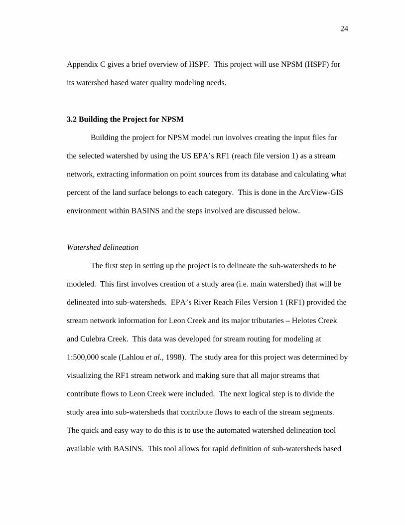
Figure 2 shows a scatter plot of observed vs. predicted flows at USGS gauging

station 08181480 on Leon Creek. R-squared value of 0.657 indicates a fairly

reasonable prediction for hydrology. The slope of the line is about 0.9.

39

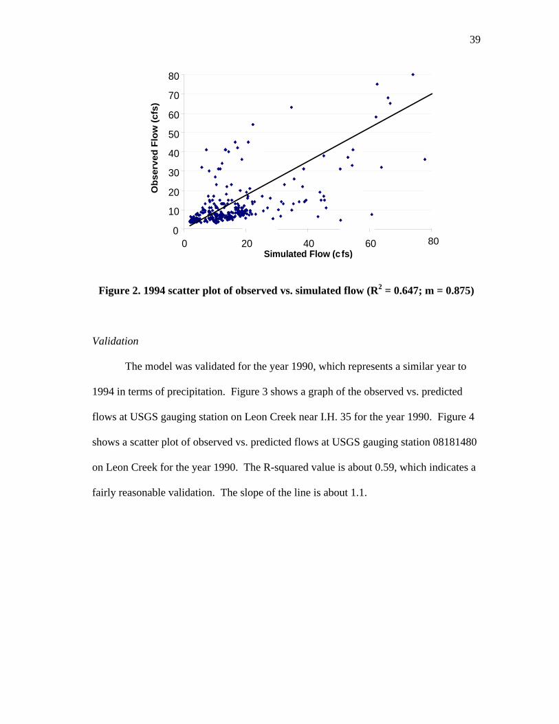
Figure 2. 1994 scatter plot of observed vs. simulated flow (R2 = 0.647; m = 0.875)

Validation

The model was validated for the year 1990, which represents a similar year to

1994 in terms of precipitation. Figure 3 shows a graph of the observed vs. predicted

flows at USGS gauging station on Leon Creek near I.H. 35 for the year 1990. Figure 4

shows a scatter plot of observed vs. predicted flows at USGS gauging station 08181480

on Leon Creek for the year 1990. The R-squared value is about 0.59, which indicates a

fairly reasonable validation. The slope of the line is about 1.1.

0

10

20

30

40

50

60

70

80

0 20 40 60 80 Simulated Flow (cfs)

Ob

se

rve

d F

low

(c

fs)

80

40

Figure 3. 1990 simulated and observed flow

0

10

20

30

40

50

60

70

80

0 10 20 30 40 50 60 70 80

Simulated Flow (cfs)

Ob

se

rve

d F

low

(c

fs)

Figure 4. 1990 scatter plot of observed vs. simulated flow (R2 = 0.59; m = 1.112)

0

100

200

300

400

500

600

700

800

J F M A M J J A S O N D

Time (Days)

Flo

w (

cfs

)

SimulatedObserved

41

Hydrology sensitivity analysis

Three model parameters that affect base flow and overall water balance

respectively were considered for sensitivity analysis. These parameters were soil

infiltration capacity (INFILT) and deep percolation losses (DEEPFR) in the Pervious

Land Module (PERLND) and retention storage capacity (RETSC) in the Impervious

Land Module (IMPLND). A simple sensitivity analysis was performed by varying the

parameters by +/- 50 percent of the calibrated values.

In NPSM/HSPF, INFILT is the parameter that controls the division of

precipitation into surface and sub-surface flow and storage compartments (BASINS

Tech. Note). Higher INFILT values means higher base flow in streams as more water

goes to the sub-surface. Lower INFILT values mean that more water flows as surface

runoff and less water percolates, leading to lower base flow. Infiltration also affects the

overall runoff volume. The more the infiltration, the higher the chance for

evapotraspiration losses from soil layers. Similarly, in conjunction with DEEPFR (deep

percolation), higher INFILT values lead to larger permanent losses from the watershed.

It was found that increasing the INFILT value by 50 percent lead to an increase of 23

percent in the overall runoff volume and an increase of 87 percent in average base flow

for the year 1994. Decreasing the INFILT value by 50 percent decreased the overall

runoff volume by 22 percent and the average base flow by 74 percent for the year 1994.

DEEPFR in NPSM/HSPF is the fraction of infiltrating water that is lost to deep

percolation. 1-DEEPFR then is the fraction available as active groundwater storage and

hence contributes to base flow in the streams. Portions of a watershed at higher

42

elevations are more prone to groundwater losses since there might be lateral outflows to

low-lying aquifers outsides the watershed. An example of this inter-watershed transfer

is the significant flow from Edward's Aquifer to Comal Springs. During 1980, nearly

48 percent of the spring discharge form Edwards Aquifer was from Comal Springs in

Comal County (Ryder, 1996). DEEPFR is also used to denote losses that may not be

measured at the flow gage used for calibration, such as flow around or under the gage

site. On account of the above reasons, DEEFR was set to 0.4, which is a rather high

value. However, it gave a reasonable water balance. A detailed study of groundwater

conditions is needed to verify this value. A 50 percent increase in DEEPFR led to a

29.6 percent decrease in overall runoff volume for the year 1994. Decreasing DEEPFR

by 50 percent increased the overall runoff volume by 41 percent for the year 1993.

RETSC is the depth of water that collects on the impervious surface before any

runoff occurs. This directly affects the amount of storm water runoff in streams and

hence the overall runoff volume. A 50 percent increase in RETSC led to a 10 percent

decrease in overall runoff volume for the year 1993. Decreasing RETSC by 50 percent

increased overall runoff volume by 14.3 percent for the year 1993. It should be noted

that RETSC does not affect base flow in the streams, but only the surface runoff from

impervious land.

Temperature

Temperature plays a significant role in the solubility of oxygen in water.

Oxygen, being a non-polar molecular compound is not highly soluble in water.

43

Solubility of oxygen depends on water temperature and salinity among others and can

range from 4ppm1 to 15ppm. Higher water temperatures demonstrate lower solubility

of oxygen and vice-versa. However, water temperature and DO are not related linearly.

To account for temperature therefore, it is necessary to consider the percentage

saturation. DO is then denoted as a percentage of the saturation value for a particular

temperature. For example, a DO concentration of 7.5 mg/l (or ppm) might represent a

90 percent saturation, which means a good turnover for DO at that particular

temperature. However the same concentration of 7.5 mg/l might represent 60 percent

saturation, thus indicating a poor turnover for that particular temperature.

Temperature of water is a linear regression function of air temperature in

NPSM. It was observed that simulated water temperature followed the air temperature

curve and was lower than the air temperature, which is usually the case for small

streams. As the volume of water is not large compared to a reservoir or lake, the water

is expected to gain and lose heat quickly and hence follow the air temperature curve in

shape. For this project, calibration for water temperature was found to be difficult for

the following reasons:

1. No hourly-observed data was available for the simulation period. Hourly data

was available for a period of two weeks in August 2000, January 2000 and July

2000 from the water quality Datasondes deployed in the creek. The data

availability constraints within BASINS and NPSM restrict the simulation of the

1 parts per million

44

model up to the year 1995. Hence, it was not possible to simulate the model for

the year 2000.

2. Some “grab sample” data was available from SARA for the years 1994-97.

However, the quantity of data was very less. For example, only 16 readings

were available for the year 1994 at the SARA monitoring site near Leon Creek

Wastewater Treatment Plant. These readings represent a “snap-shot” of the

water conditions at a particular time of the day and by no means represent the

hourly values or even daily means. Thus, this data set is of practically no use for

calibration purposes. Moreover, the location of data collection was different

from the location of the calibration point, although it was on the same stream

segment as the calibration point. Depending on the conditions surrounding the

sampling points, the data can vary considerably within the same reach segment.

For example, the water temperatures at a location surrounded by shade can be

lower than a down stream or upstream location where there is no shade.

Considering the above factors, it is evident that calibration for temperature is a

not possible for the present study. The same holds true for DO. Moreover, the aim of

the project was not to use the model for deterministic analysis, but rather to analyze

trends. Using a complex and highly parameterized model such as NPSM (HSPF) itself

involves a big learning curve, much less using it to simulate such a complex constituent

as DO. The objective of the project was to be able to use NPSM to successfully

simulate the various physical, chemical and biological processes taking place in the

45

watershed and to compare simulated trends with the trends actually observed. In other

words, the objective was to see how effective the model simulates complex processes,

rather than how accurately it does it. Extensive calibration therefore was neither a

priority nor a possibility within the given time frame and data constraints. In absence of

calibration, a trend analysis is the best option to determine whether the model is doing

what it is supposed to do.

Dissolved Oxygen

As pointed in the earlier section, calibration for DO is not possible for the

present study. From the standpoint of the NPSM model, what is of importance however

is whether that model can simulate diurnal DO variations within a stream segment. For

the purpose of trend analysis, the data collected using Datasondes at the sampling site

on Lackland Airforce Base was used. January and July 2000 data was chosen to

represent cold and hot weather conditions. As explained in the previous section, the

model could not be setup for year 2000 simulation period. Hence, the 1994 water year

was chosen for simulation of DO with the model. 1994 happens to be the most recent

year that has similar precipitation and flow trends as the year 2000. The following

criteria were used:

1. Annual precipitation comparison

2. Monthly precipitation comparison

3. Mean daily stream flow comparison during the period for which data was

collected using Datasondes.

46

Appendix G shows the comparison charts for the above criteria. Various

module sections within NPSM were chosen to simulate DO. These represent to a large

extent, almost all of the complex processes taking place in the watershed and in the

streams. These processes include fate and transport of BOD and nutrient loading on

land surfaces, benthal oxygen demand, phytoplankton influences, alga respiration and

sediment oxygen demand among others. Appendix H shows the NPSM simulation

module matrix for DO simulation. Appendix I shows the DO parameter definition table

for NPSM. The table also gives the default values and the maximum and minimum

values as defined for the model. A few parameters were changed from their default

values. Their values are also given in Appendix I. Quantities such as BOD and nutrient

application rates were supplied by the user since there were no default values. Nutrient

application rates were estimated from a report of the United States Department of

Agriculture (UDSA) (Lander and Moffit, 1996). These rates were chosen just to

demonstrate that nutrient and BOD loading processes could be simulated by NPSM.

The model was then run for the simulation period 1994. Figure 5 shows simulated

hourly DO for January 1994 as compared to observed hourly DO for January 2000

during the period starting 26th January and ending 31st January. Similarly, Figure 6

shows simulated hourly DO for July 1994 as compared to observed hourly DO for July

2000 during the period starting 26th July and ending 29th July.

47

Figure 5. 1994 simulated and 2000 observed hourly DO during Jan. 26 to Jan. 31

Figure 6. 1994 simulated and 2000 observed hourly DO during Jul. 26 to Jul. 29

0

2

4

6

8

10

12

0 20 40 60 80 100 120 140 160

Time (Hours)

DO

(m

g/l)

ObservedSimulated

0

2

4

6

8

10

12

0 20 40 60 80 100

Time (Hours)

DO

(mg/

L)

SimulatedObserved

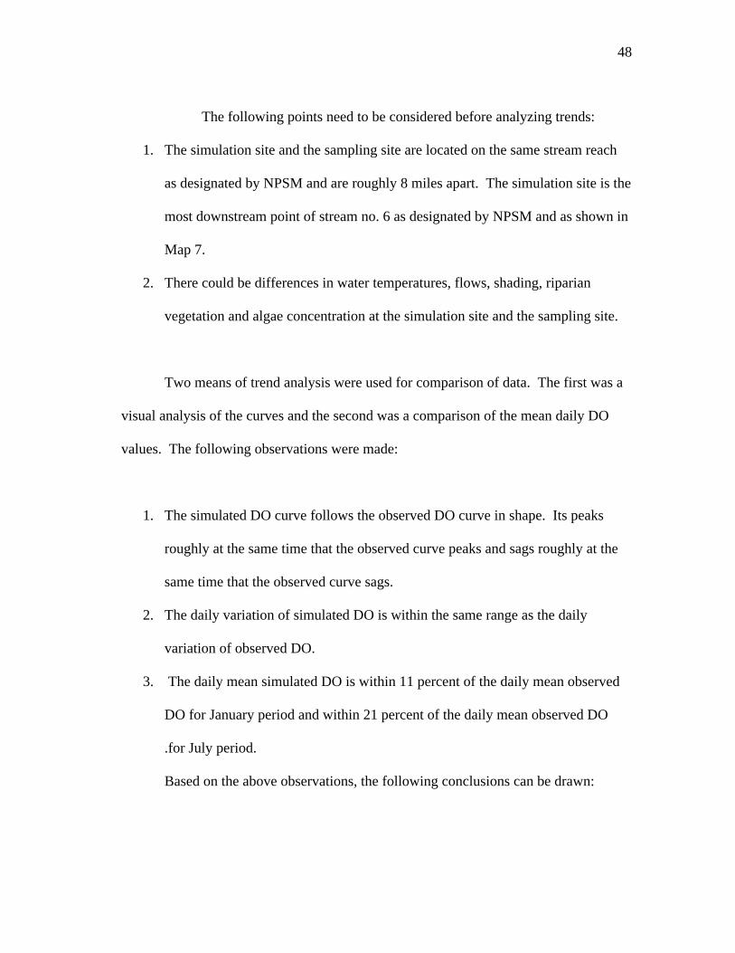
48

The following points need to be considered before analyzing trends:

1. The simulation site and the sampling site are located on the same stream reach

as designated by NPSM and are roughly 8 miles apart. The simulation site is the

most downstream point of stream no. 6 as designated by NPSM and as shown in

Map 7.

2. There could be differences in water temperatures, flows, shading, riparian

vegetation and algae concentration at the simulation site and the sampling site.

Two means of trend analysis were used for comparison of data. The first was a

visual analysis of the curves and the second was a comparison of the mean daily DO

values. The following observations were made:

1. The simulated DO curve follows the observed DO curve in shape. Its peaks

roughly at the same time that the observed curve peaks and sags roughly at the

same time that the observed curve sags.

2. The daily variation of simulated DO is within the same range as the daily

variation of observed DO.

3. The daily mean simulated DO is within 11 percent of the daily mean observed

DO for January period and within 21 percent of the daily mean observed DO

.for July period.

Based on the above observations, the following conclusions can be drawn:

49

1. The model is capable of simulating the diurnal variation of DO for a stream

segment.

2. For the scope of the present study, the DO simulation done by the model is

satisfactory.

3. The model presently cannot accurately reproduce the diurnal swings in DO in

amplitude. This might be due to the fact that simulated organic loading, nutrient

loading and algal concentrations in the streams is not representative of real

conditions. With extensive calibration and continuous sampling data, the

simulation curve could be improved to represent actual conditions.

Sensitivity analysis for DO

Simulation of the entire DO source and sink cycle in a stream is highly complex

and requires an in-depth understanding of in-stream processes. These include BOD,

BOD settling, sediment oxygen demand, benthic influences, algal respiration and

photosynthesis among others. Besides, these processes can vary significantly along the

length of a stream depending on local conditions such as flow, land-use, shading and

nutrient loading. Surface processes such as the BOD loading and washoff, nutrient

application and washoff, plant uptake of nutrients and atmospheric deposition of

nitrogen compounds also indirectly affect the in-stream processes. NPSM has the

capability of simulating all these processes involving a large number of parameters.

Understanding enough about these parameters in order to get calibrated values involves

extensive research that is often not possible due to time constraints or lack of data. As

50

such, there is an inherent uncertainty built in the model because of over-

parameterization.

Due to the above reasons, it was though best to keep default values for most in-

stream parameters that affect DO. A few parameters were changed from their default

values and their values are given in Appendix I. Performing a detailed sensitivity

analysis was beyond the scope of this project. It was however found that in-stream DO

concentration was extremely sensitive to groundwater concentration of DO. This is

reasonable since groundwater recharges Leon Creek via springs. A simple sensitive

analysis was performed by varying the groundwater DO concentration (GRNDDOX) by

+/-50 percent from the calibrated monthly values. An increase of 50 percent in

GRNDDOX led to an average increase of 35 percent in the predicted average daily DO

concentration during the period January 26, 1994 to January 31 1994. Decreasing

GRNNDOX by 50 percent led to a 44.5 percent decrease in average daily DO

concentration over the same period. Similarly, an increase of 50 percent in GRNDDOX

led to an average increase of 12.7 percent in the predicted average daily DO

concentration during the period July 26, 1994 to July 29, 1994. Decreasing

GRNNDOX by 50 percent led to a 20.8 percent decrease in average daily DO

concentration over the same period.

51

3.5 Low-flow Augmentation to Rectify DO Problems: A Rehabilitation Approach

Introduction

The ultimate objective of this project was to evaluate the effects of low flow

augmentation on the DO concentration of Leon Creek. As stated earlier, most of the

DO problems in streams occur during low flow conditions when the water is stagnant,

the concentration of nutrients, algae and BOD is high and the reaeration rate is low.

The July 2000 observed DO graph (Figure 6) is an example of such conditions. It

shows that the DO criterion was violated at many instances with concentrations as low

as 4.3 mg/l. Such low flow conditions usually occur during dry periods when there is

no rainfall and the temperatures are hot. It should be noted that Texas experienced one

of the hottest summers that year with record temperatures and record number of

consecutive days without significant precipitation.

The city of San Antonio boasts of a history of water recycling dating back to the

1960s when the city public service (CPS), the electric utility started using treated

wastewater from the Calaveras and Braunig lakes in its cooling towers (Texas Water

Savers, 1998). In the recent years, in an effort to maintain the sustainability of

Edward’s Aquifer, SAWS started to develop the San Antonio Water Recycling Project.

As part of this project, treated wastewater from the Leon Creek Waste Water Treatment

Plant (see map 8 of Appendix A) will be used for irrigation, instream flows and

industrial purposes. Pipelines painted in purple have already been installed. In a pilot

project in 1996, water treated at the Leon Creek plant and stored at Lake Mitchell was

delivered to Mission del Lago Golf Course for irrigation purposes. The Water

52

Recycling Project is expected to save about 11 billion gallons of Edwards Aquifer water

annually for potable use (Texas Water Savers, 1998).

Approach

For the present study, a hypothetical quantity of water having quality

representative of the Leon Creek Wastewater Treatment Plant discharge was assumed to

be conveyed from the plant to an upstream site via the recycling pipe. This treated

wastewater was discharged at an arbitrarily chosen upstream point to augment in-stream

flow. This scenario can be represented in NPSM by adding a “point source” to the

stream of interest. The exact location of the point source can be specified by entering a

“mile point” number i.e. the number of miles from the most downstream point on the

stream of interest. For the present study, stream segment number 5 (Culebra Creek) in

NPSM was chosen as the receiving stream for flow augmentation. The mile point for

the point source was fixed at 3.75 miles, which is the headwater for the creek. Map 8 of

Appendix A shows the point of application of flow and the point at which water quality

was measured by the model. Four parameters were chosen to represent the quality of

water entering as point source in NPSM. These were nitrate-nitrogen, phosphate

(dissolved ortho-phosphorus), DO and BOD. Representative values for nitrate-nitrogen

and phosphate were obtained from the data obtained from SARA at its monitoring site

located near the treatment plant. No data for BOD concentration were available from

SARA. BOD data was acquired from effluent data collected by the San Antonio Water

System (SAWS) monitoring site near the treatment plant. Annual average BOD

53

concentration for the 6-year period 1992-98 was used as a representative value. Table 6

shows the representative values for water quality for the Leon Creek Wastewater

Treatment Plant discharge.

Table 6. Representative values for water quality constituents at Leon Creek WWTPConstituent Concentration/ValueBOD 2.25 mg/lNitrate Nitrogen 5.5 mg/lPhosphorous (Phosphate) 1.3 mg/lTemperature 27 o CPH 7.0Dissolved Oxygen 7.0 mg/l

Scenario analysis

A 3-month period with no significant rainfall was chosen between 1st July and

30th September of years 1993, 1994 and 1995. This constituted a hot weather low-flow

period as compared to other months. The periods were chosen based on the following

four criteria:

1. Palmer Drought Severity Index

2. Monthly mean precipitation as observed at San Antonio International

Airport.

3. Monthly mean temperatures as observed at San Antonio International

Airport.

4. Monthly mean observed flows as observed at USGS gauging station

number 08181480, which was used for hydrology calibration.

54

Appendix J gives an explanation as well as graphical representation of the above

criteria. Six scenarios were evaluated. They are as follows:

1. Control (CTRL) – Simulated flow and DO without any external flow source.

This is the “as is” scenario.

2. Scenario 1 (S1) – Flow augmented by adding a point source with 0.25 times

base flow.

3. Scenario 2 (S2) – Flow augmented by adding point source with 0.5 times

base flow.

4. Scenario 3 (S3) – Flow augmented by adding point source with 1 times base

flow.

5. Scenario 4 (S4) - Flow augmented by adding point source with 2 times base

flow.

6. Scenario 5 (S5) - Flow augmented by adding point source with 4 times base

flow.

Daily mean DO concentrations were then calculated by averaging over the 24-

hour period for each day, for 92 days. Plots of daily mean DO for each scenario during

the 1993, 1994 and 1995 study periods are shown in figures 7, 8 and 9 respectively.

55

Figure 7. Daily mean DO during 1993 scenario analysis

Figure 8. Daily mean DO during 1994 scenario analysis

5

6

7

8

9

10

11

12

0 20 40 60 80 100

Time (Days) 07/01 to 09/30

DO

(mg/

l)CONTROLSCEN01SCEN02SCEN03SCEN04SCEN05

5

6

7

8

9

10

11

12

0 20 40 60 80 100

Time (Days) 07/01 to 09/30

DO

(mg/

l)

CONTROLSCEN01SCEN02SCEN03SCEN04SCEN05

56

Figure 9. Daily mean DO during 1995 scenario analysis

To evaluate the scenarios, statistical analysis was performed using the Statistical

Analysis System (SAS) software. The sample population consisted of 92 data points for

each scenario. Each data point represented the daily mean DO concentration in mg/l

over the chosen three-month low-flow period for 1993, 1994 and 1995. Following

methods were used for comparison of the datasets and means:

1. Kruskal-Wallis Chi-Square Approximation Test – Pre-test for

differences.

2. Student-Neuman-Keuls (SNK) Test

3. Tukey’s Studentized Range (HSD) Test

The output of statistical analysis is given in appendix K.

5

6

7

8

9

10

11

12

0 20 40 60 80 100

Time (Days) 07/01 to 09/30

DO

(m

g/l)

CONTROLSCEN01SCEN02SCEN03SCEN04SCEN05

57

CHAPTER IV

RESULTS AND DISCUSSION

4.1 Statistical Analysis of Scenarios

Box plots of the six scenarios depicting the treatment type (quantity of flow

augmentation) as the predictor variable (X) and daily mean DO (mg/l) as the response

variable (Y) are shown in figures 10, 11 and 12 below.

Figure 10. Box plot for 1993 scenario analysis

58

Figure 11. Box plot for 1994 scenario analysis

Figure 12. Box plot for 1995 scenario analysis

It can be incurred from the box plots that the data from the sample populations is

not normally distributed. Most of the sample populations are skewed and some of them

are heavily tailed. A visual comparison of the box plots shows that there is a

considerable overlapping between the first four populations (CTRL, S1, S2 and S3).

However, sample population S5 shows a significantly different mean than the rest. This

suggests that the null hypothesis (H0 = all means are equal) is not true. A statistical

59

basis for arriving at this conclusion is the one-way analysis of variance (one-way

ANOVA) test. However, the one-way ANOVA test assumes that the data is normally

distributed. Since the sample populations are not normally distributed, an alternative

test called the Kruskal-Wallis Test was used. The Kruskal-Wallis Test is good for data

that is highly skewed. Moreover it is a non-parametric test, i.e. it makes no assumption

about population distribution. It tests the following two hypotheses:

H0 (Null hypothesis) = All k populations have the same distribution

H1 = Data from some populations tend to be larger than data from others.

From the SAS output of Kruskal-Wallis test in Appendix L, it was observed that

with a 95% confidence level (_ = 0.05), the p-value (i.e. probability > Chi-square) was

less than _ for all three periods. Hence the null hypothesis was rejected and it was

concluded that some means differ. To find which means differ, the Student-Newman-

Keuls Test and the Tukey’s Studentized Range Test were performed in SAS. A

confidence level of 95% (_ = 0.05) was set for the tests. SAS output for the test is

provided in Appendix L. Table 7 gives a summary of the statistical analysis.

60

Table 7. Summary of statistical analysis of augmentation scenarios

1993 1994 1995

Scenario Description Rank SNKGrouping

TukeyGrouping

SNKGrouping

TukeyGrouping

SNKGrouping

TukeyGrouping

CONTROL “As is” 6 E

E

D

D

F E F E

S1 0.25 times base-flow (1.25 cfs*)

5 E D

D

D

D

E D

D

E D

D

S2 0.5 times base-flow(2.5cfs)

4 D D D D D D

S3 1 times base-flow(5 cfs)

3 C C C C C C

S4 2 times base-flow(10 cfs)

2 B B B B B B

S5 4 times base-flow(20 cfs)

1 A A A A A A

Note:

1. Average base flow for the study period during 1993, 1994, and 1995 was taken as 5 cfs.

2. Scenarios are ranked in descending order of mean daily DO for the sample populations.

3. Means with the same letter are not significantly different.

* cubic feet per second

61

From the output the following observations were made:

Student-Newman-Keuls Test

1. The daily mean DO concentration for the sample population increases with

increasing flows; i.e. S5 > S4 > S3 > S2 > S1 > CTRL.

2. 1993 scenario analysis showed no significant difference in mean DO for the

Control, S1 and S2 scenarios. A significance difference in means is observed

from scenario S3 onwards.

3. 1994 scenario analysis showed a significant difference in mean DO for all

scenarios.

4. 1995 scenario analysis showed a significant difference in mean DO for all

scenarios.

Tukey’s Studentized Range Test

1. Daily mean DO concentration for the sample population increases with

increasing flows; i.e. S5 > S4 > S3 > S2 > S1 > CTRL.

2. 1993 scenario analysis showed no significant difference in mean DO for the

Control, S1 and S2 scenarios. A significance difference in means is observed

from scenario S3 onwards.

62

3. 1994 scenario analysis showed no significant difference in mean DO for

scenarios S1 and S2. All other scenario means were significantly different from

each other.

4. 1995 scenario analysis showed no significant difference in mean DO for

scenarios S1 and S2. All other scenario means were significantly different from

each other.

Another important observation that was made from the box plots is that for

1994, scenario S1 and S2 as well as the control scenario had some data point that

fell below the DO criteria of 5 mg/l. Similarly for 1995, some data point in the

control scenario (CTRL) fell below 5mg/l where as some data point in scenario S1

were close to 5mg/l.

4.2 Interpretation of Results: Effects of Low-flow Augmentation

From the statistical analysis, the following conclusions can be made:

1. Increasing the flow in streams increases the mean daily DO concentration during

low flow periods for the years 1993, 1994 and 1995

2. Scenarios S1 and S2 are not significantly different from each other and both

show an increase in mean daily DO concentration as compared to the control

scenario. However since some data points in S1 and S2 fall below DO criteria

of 5 mg/l during at least one low-flow period (1994), they are not acceptable.

63

3. Scenario S3 shows a significantly different mean than scenarios S2 and S3 and

also none of the data points in S3 fall below 5 mg/l. The same is true for S4 and

S5. Hence it can be concluded that one can see a significant change (increase)

in mean daily DO concentration from scenario S3 onwards.

4. Since the significance level of the tests was set to _ = 0.05, one can be 95%

confident of the overall multiple comparison of means. This means that the

confidence level for comparison of any two means in the ANOVA data set is

greater than 95%. Hence, one can be more than 95% confident in saying that

scenario S3 has a significantly greater mean DO than scenarios CTRL, S1 and

S2 compared one at a time. Same holds true for comparing S4 and S5 with

CTRL, S1, S2 and S3 respectively, one at a time.

One should note from the above discussion that scenario S3 defines a “threshold

response”, meaning a significant change in the system is observed from scenario S3

onwards (with a certain confidence level). A watershed level modeling of DO is a

highly complex process fraught with uncertainty in data, parameter estimation (because

of lack of knowledge of various processes) and model performance. Hence, in order to

be more certain of observing a positive change in system response, scenarios beyond the

threshold response scenario should be considered strongly. Referring to figures 7, 8 and

9 in chapter III, one can visually interpret the response of a complex system. One can

see that the system behaves linearly for scenarios S1, S2 and S3 and starts showing non-

linear response from scenario S4 onwards. Scenario S5 shows a significantly different

64

response for all three years whereas scenario S4 shows a significantly different response

for the year 1994.

4.3 Feasibility of Scenario Implementation

The total capacity of Leon Creek Wastewater Treatment Plant is about 32mgd2.

About 26mgd of this treated wastewater is earmarked for recycling purposes. The rest

will be split up for downstream release and for delivery to Mitchell Lake. The recycling

pipes are 42 inches in diameter and designed to deliver 26mgd of treated wastewater to

various customers all year round. This translates to a flow of about 40.3 cfs. Hence,

the flow augmentation scenarios of 5 cfs (S3), 10 cfs (S4) and 20 cfs (S5) for the three-

month period can be implemented without any additional pumping or infrastructure

costs to the City. As of now, no quantity of recycled water has been earmarked for in

stream releases from the Leon Creek Water Recycling Center. Whether the City can

allocate recycled water for flow augmentation depends on its commitments to other

customers and is an issue that is beyond the scope of this study.

2 million gallons per day

65

CHAPTER V

CONCLUSIONS AND RECOMMENDATIONS

The hypothesis tested in this study was that increasing dry period base flow in

streams by discharge from a wastewater treatment plant (with pre-defined water quality

parameters) enhances water quality in terms of DO. This has been demonstrated to be

the case. An increase in daily mean DO was observed for all treatment scenarios tested.

With 95 % confidence level, a significant change was observed with scenario S3 (one

times base flow), i.e. doubling the base flow during low-flow periods. This constitutes

a risk-based design approach to remedy DO problems by low-flow augmentation. In

other words, we can say with 95% confidence that a minimum flow augmentation of

one times base flow can remedy DO problems during dry, low-flow periods. This

amounts to a discharge of 5 cfs during each three-month period. As mentioned in the

previous chapter, the various flow augmentation alternatives are well within the

capacity of the plant.

As stated in chapter IV, scenario S3 defines the “threshold response” of a

complex system fraught with uncertainty. Hence, to increase the chances of seeing a

significant improvement in the system, scenarios S4 or S5 are highly recommended. As

is evident, these alternatives are also within the capacity of the plant.

The basis of the above hypothesis is that the treatment plant discharge has a pre-

defined water quality. The above hypothesis might not hold true for any wastewater

66

treatment plant discharge. In fact, in all probability, the hypothesis will fail if there is

increasing organic and nutrient burden (higher BOD, nitrates and phosphates) from the

discharge. Studying the diurnal swings of DO cycle can assess the effects of such

burden.

From a design consideration standpoint, carrying wastewater in pipelines to the

point of flow-augmentation will completely strip it of its DO content. Therefore a

passive entrainment aeration system is highly recommended at the point of discharge so

that plenty of oxygen is available to aquatic organisms before the water enters the

stream. This can be accomplished using gravity powered entrainment devices such as

cascade- reaeration. Potential odor problems must be given consideration before

deciding on a reaeartion process. However, given the quality of the water (Type I, the

highest grade effluent), odor problems are not likely to occur.

Presently, the model is loosely calibrated for hydrology as well as DO. Besides,

A very simplistic built-up and wash-off process was simulated for BOD and nutrient

loading from land surfaces. This might not represent true conditions. As such, for now

the model is good for predicting trends and cannot accurately simulate diurnal swings.

Lack of historic data for DO is also a factor that limited model calibration. A detailed

knowledge of nitrogen and phosphorus cycle on land surfaces, and in stream processes

such as reaeration, algal respiration rate, sediment oxygen demand and algal growth

among others is required for better model performance. Availability of representative

precipitation data is also very crucial since the model is driven by precipitation.

67

The project demonstrated that the Non Point Source Model (NPSM), is capable

of simulating watershed processes as well as in-stream processes and is good for a

screening level analysis of scenarios and trends. However the model is extensively

parameterized and requires a big learning curve for detailed studies. Thus

comprehensive data requirements, overparametrization, lack of detailed knowledge and

time constraints have limited the model performance. Moreover, the DO simulation

process using NPSM has not been documented in detail in literature or elsewhere. As

such, the model is fraught with bugs that are known only to a few experts. Some bugs

were encountered during model use and they have been documented in Appendix K.

As stated earlier, a screening level analysis was performed to evaluate scenarios

and observe trends. It is recommended that a more detailed analysis be carried out

using a steady-state in stream water quality model such as QUAL2E. DO conditions

can then be studied in detailed segment by segment there by giving a longitudinal

resolution to water quality that is not possible using NPSM. This way, specific lengths

of the creek that have low-flow DO problems can be identified and scenarios evaluated.

Finally, there is uncertainty involved in any modeling process. This uncertainty

gets translated in model predictions. Therefore, it is critical for decision-makers to be

cognizant of this uncertainty before making decisions based on model performance.