igor/publication/cialencoandbi2011counterparty...counterparty risk and the impact of...
TRANSCRIPT

Counterparty Risk and the Impact of Collateralization
in CDS Contracts
Tomasz R. Bielecki∗
Department of Applied Mathematics,
Illinois Institute of Technology,
Chicago, 60616 IL, USA
Igor Cialenco∗
Department of Applied Mathematics,
Illinois Institute of Technology,
Chicago, 60616 IL, USA
Ismail Iyigunler
Department of Applied Mathematics,
Illinois Institute of Technology,
Chicago, 60616 IL, USA
April 13, 2011
Abstract
We analyze the counterparty risk embedded in CDS contracts, in presence of a bilateral margin
agreement. First, we investigate the pricing of collateralized counterparty risk and we derive the bilat-
eral Credit Valuation Adjustment (CVA), unilateral Credit Valuation Adjustment (UCVA) and Debt
Valuation Adjustment (DVA). We propose a model for the collateral by incorporating all related factors
such as the thresholds, haircuts and margin period of risk. We derive the dynamics of the bilateral CVA
in a general form with related jump martingales. We also introduce the Spread Value Adjustment (SVA)
indicating the counterparty risk adjusted spread. Counterparty risky and the counterparty risk-free
spread dynamics are derived and the dynamics of the SVA is found as a consequence. We finally employ
a Markovian copula model for default intensities and illustrate our findings with numerical results.
∗TRB and IC acknowledge support from the NSF grant DMS-090809
1

Contents
1 Introduction 2
2 Pricing Counterparty Risk: CVA, UCVA and DVA 3
2.1 Dividend Processes and Marking-to-Market . . . . . . . . . . . . . . . . . . . . . . . . . . . . 4
2.2 Bilateral Credit Valuation Adjustment . . . . . . . . . . . . . . . . . . . . . . . . . . . . . . . 7
2.2.1 Unilateral CVA and Debt Value Adjustment . . . . . . . . . . . . . . . . . . . . . . . 9
2.2.2 CVA via Credit Exposures . . . . . . . . . . . . . . . . . . . . . . . . . . . . . . . . . 10
2.3 Dynamics of CVA . . . . . . . . . . . . . . . . . . . . . . . . . . . . . . . . . . . . . . . . . . 11
2.3.1 Dynamics of CVA when the immersion property holds . . . . . . . . . . . . . . . . . . 18
2.4 Fair Spread Value Adjustment . . . . . . . . . . . . . . . . . . . . . . . . . . . . . . . . . . . 18
2.4.1 SVA Dynamics . . . . . . . . . . . . . . . . . . . . . . . . . . . . . . . . . . . . . . . . 20
3 Multivariate Markovian Default Model 22
3.1 Results . . . . . . . . . . . . . . . . . . . . . . . . . . . . . . . . . . . . . . . . . . . . . . . . . 22
4 Conclusion 23
1 Introduction
Not very long after the collapse of prestigious institutions like Long-Term Capital Management, Enron and
Global Crossing, the financial industry has again witnessed dramatic downfalls of financial institutions such
as Lehman Brothers, Bear Stearns and Wachovia. These recent collapses have stressed out the importance
of measuring, managing and mitigating counterparty risk appropriately.
Counterparty risk is defined as the risk that a party in an over-the-counter (OTC) contract will default
and will not be able to honor its contractual obligations. Since the exchange-traded derivative contracts are
subject to clearing by the exchange, counterparty risk arises from OTC derivatives only. The main challenge
in the counterparty risk assessment and hedging is that the exposures of OTC derivatives are stochastic and
involve dependencies and systemic risk factors such as wrong way risks; the additional level of complexity is
introduced by risk mitigation techniques such as collateralization and netting. Therefore, one needs to model
potential future exposures and to price the counterparty risk appropriately according to margin agreements
that underlie the collateralization procedures.
In this paper, we analyze the counterparty risk in a Credit Default Swap (CDS) contract in presence
of a bilateral margin agreement. There are three risky names associated with the contract: the reference
entity, protection seller (the counterparty) and the protection buyer (the investor). Contrary to the common
approach which starts with defining the Potential Future Exposure (PFE) and derives the Credit Valuation
Adjustment (CVA) as the price of the counterparty risk, we find the CVA as the difference between the
market values of a counterparty risk-free and a counterparty risky CDS contracts and deduct the relevant
credit exposures accordingly. We consider the problem of bilateral counterparty risk assessment; that is,
we consider the situation where the two counterparties of the CDS contract , i.e. the investor and the
counterparty, are subject to default risk in a counterparty risky CDS contract.
2

We focus on the collateralized contracts, where, as a vital risk mitigation tool, a bilateral margin agree-
ment is in force, and it requires the counterparty and the investor to post collateral in case their exposure
exceeds specific threshold values. We propose a model for the collateral by incorporating all related factors,
such as thresholds, margin period of risk and minimum transfer amount. Then, we derive the dynamics
of the bilateral CVA which is essential for dynamic hedge of the counterparty risk. We also compute the
decomposition of the fair spread for the CDS, and we analyze so called Spread Value Adjustment (SVA).
Essentially, SVA represents the adjustment to be made to the fair spread to incorporate the counterparty
risk into the CDS contract.
Using the bilateral CVA formula, we derive relevant formulas for assessment of credit exposures, such as
PFE, Expected Positive Exposure (EPE) and Expected Negative Exposure (ENE).
In our model, the dependence between defaults and the wrong way risk is represented in a Markovian
copula framework that accounts for simultaneous defaults among the three names represented in a CDS
contract. In this way, our model takes broader systemic risk factors into account and quantifies the wrong
way risk and the double defaults in a tangible manner.
This paper is organized as follows. In section 2, we first define the dividend processes regarding the
counterparty risky and the counterparty risk-free CDS contract in case of a bilateral margin agreement. We
also define the CVA, UCVA and the DVA terms as well as the credit exposures such as PFE, EPE and ENE.
We then prove the dynamics of the CVA in section 3. Moreover, we find the fair spread adjustment term
and its dynamics. In section 4, we simulate the collateralized exposures and the CVA using our Markovian
copula model of default dependence.
2 Pricing Counterparty Risk: CVA, UCVA and DVA
We consider a standard CDS contract, and we label by 1 the reference name, by 2 the counterparty (the
counterparty), and by 3 the investor. Each of the three names may default before the maturity of the CDS
contract, and we denote by τ1, τ2 and τ3 their respective default times. These times are modeled as non-
negative random variables given on a underlying probability space (Ω,G,Q). We let T and κ to denote the
maturity and the spread of our CDS contract, respectively. We assume the recovery at default covenant;
that is, we assume that recoveries are paid at times of default.
We introduce right-continuous processes Hit by setting Hi
t =Iτi≤t and we denote by Hi the associated
filtrations so that Hit = σ
(Hi
u : u ≤ t)for i = 1, 2, 3.
We assume that we are given a market filtration F, and we define the enlarged filtrationG = F∨H1∨H2∨H3,
that is Gt = σ(Ft ∪H1
t ∪H2t ∪H3
t
)for any t ∈ R+. For each t ∈ R+ total information available at time t is
captured by the σ-field Gt. In particular, processes Hi are G-adapted and the random times τi are G-stopping
times for i = 1, 2, 3.
Next, we define the first default time as the minimum of τ1, τ2 and τ3: τ = τ1∧ τ2∧τ3; the corresponding
indicator process is Ht = Iτ≤t. In addition, we define the first default time of the two counterparties:
τ∗= τ2 ∧ τ3, and the corresponding indicator process H∗t = Iτ∗≤t.
We denote by Bt the savings account process, that is
Bt = e∫ t0rsds,
3

where the F-progressively measurable process r models the short-term interest rate. We also postulate that
Q represents a martingale measure associated with the choice of the savings account B as a discount factor
(or numeraire).
2.1 Dividend Processes and Marking-to-Market
In this paper, all cash flows and the prices are considered from the perspective of the investor.
We start by introducing the counterparty-risk-free dividend process D, which describes all cash flows
associated with a counterparty-risk-free CDS contract; 1 that is, D does not account for the counterparty
risk.
Definition 2.1 The cumulative dividend process D of a counterparty risk-free CDS contract maturing at
time T is given as,
Dt =
∫]0,t]
δ1udH1u − κ
∫]0,t]
(1−H1
u
)du, (1)
for every t ∈ [0, T ], where δ1 : [0, T ] → R is an F-predictable processes.
Process δ1 represents the loss given default (LGD); that is δ1 = 1 − R1t , where R1 is the fraction of
the nominal that is recovered in case of the default of the reference name. We assume unit nominal, for
simplicity.
The ex-dividend price processes of the counterparty risk-free CDS contract, say S, describes the current
market value, or the mark-to-market value this contract,
Definition 2.2 The ex-dividend price process S of a counterparty risk-free CDS contract maturing at time
T is given by,
St = BtEQ
(∫]t,T ]
B−1u dDu
∣∣∣∣∣Gt
), t ∈ [0, T ]. (2)
Remark 2.3 Accordingly, we define the cumulative (dividend) price process, say S, of a counterparty risk-
free CDS contract as
St = St +Bt
∫]0,t]
B−1u dDu, t ∈ [0, T ].
Now, we are in position to define the dividend process DC of a counterparty risky CDS contract, that
is the CDS contract that accounts for the counterparty risk associated with the two counterparties of the
contract.
Definition 2.4 The dividend process DC of a T -maturity counterparty-risky CDS contract is given as
DCt =
∫]0,t]
CudHu +
∫]0,t]
δ1u (1−Hu−) dH1u +
∫]0,t]
δ2u (1−Hu−) dH2u
+
∫]0,t]
δ3u (1−Hu−) dH3u +
∫]0,t]
δ4u (1−Hu−) d[H2, H3
]u
(3)
+
∫]0,t]
δ5u (1−Hu−) d[H∗,H1
]u− κ
∫]0,t]
(1−Hu) du, t ∈ [0, T ],
1We shall sometimes refer to such contract as to the clean contract.
4

where δi : [0, T ] → R is F-predictable processes for i = 1, . . . , 5 and C : [0, T ] → R is a F-predictable process
representing the collateral amount kept in the margin account.
Margin account is a contractual tool that supplements the CDS contract so to reduce potential losses
that may be incurred by one of the counterparties in case of the default of the other counterparty, while the
CDS contract is still alive. For the detailed description of the mechanics of the collateral formation in the
margin account we refer to section 2.2 (see also [BC11]).
In case of any credit event, associated with the collateralized CDS contract, the first cashflow that takes
place is “transfer” of the collateral amount; for example, in case when the underlying entity defaults at time
t = τ = τ1, (before any of the counterparties defaults) the collateral in the margin account is acquired by
one of the counterparties (depending on the sign of Cτ ). Thus, consistently with the conventions of the so
called close-out cashflows (cf. [BC11]) we define δis as follows:
• We set δ1t = δ1t −Ct. This is because after the collateral transfer the counterparty pays the remaining
recovery amount δ1t − Ct.
• At time t = τ = τ2, when the counterparty defaults, then, after the collateral transfer takes place, if the
uncollateralized mark-to-market (MtM) of the CDS contract is negative, that is if St+It=τ1δ1t −Ct <
0, 2 the investor closes out the position by paying the defaulting counterparty the uncollateralized MtM.
If the uncollateralized MtM is positive, the investor closes out the position and receives a fraction R2
of the uncollateralized MtM from the counterparty. Therefore, in this case, the close-out payment is
defined as,
δ2t = R2
(St + It=τ1δ
1t − Ct
)+ −(St + It=τ1δ
1t − Ct
)−.
• In case of investor default, that is at time t = τ = τ3, if the uncollateralized MtM is positive, that is if
St + It=τ1δ1t −Ct > 0, the counterparty closes out the position by paying the uncollateralized MtM.
If the uncollateralized MtM is negative, the counterparty receives a fraction R3 of the uncollateralized
MtM. Hence, the close-out payment is defined as,
δ3t =(St + It=τ1δ
1t − Ct
)+ −R3
(St + It=τ1δ
1t − Ct
)−.
• If the investor and the counterparty default simultaneously at time t = τ = τ2 = τ3, if the uncollater-
alized MtM negative, the counterparty receives a fraction R3 of the uncollateralized MtM; however, if
the uncollateralized MtM is positive, the investor receives a fraction R2 of the uncollateralized MtM.
Therefore, we set,
δ4t = −(St + It=τ1δ
1t − Ct
).
• If t = τ = τ∗ = τ1, that is when the investor or the counterparty default simultaneously with the
reference entity, investor receives a fraction R2 of the remaining recovery amount,(δ1t − Ct
)+, when
the counterparty defaults. Likewise, if the investor defaults, the counterparty receives a portion R3
of the remaining recovery amount,(δ1t − Ct
)−. The close-out payment in joint defaults including the
underlying entity has the form,
δ5t = −(δ1t − Ct
).
2The term It=τ1δ1t represents the exposure in case when the counterparty and the underlying entity default simultaneously.
5

We are now ready to define the price processes associated with a counterparty risky CDS contract.
Definition 2.5 The ex-dividend price process SC of a counterparty risky CDS contract maturing at time T
is given as,
SCt = BtEQ
(∫]t,T ]
B−1u dDC
u
∣∣∣∣∣Gt
), t ∈ [0, T ]. (4)
The cumulative price process SC of a counterparty risky CDS contract is given by,
SCt = SC
t +Bt
∫]0,t]
B−1u dDC
u , t ∈ [0, T ].
The counterparty posts collateral when the investor makes a margin call, which happens when investor’s
exposure exceeds the counterparty’s threshold plus the MTA. Likewise, the investor delivers collateral when
the counterparty makes a margin call, which happens when protection seller’s exposure to the buyer exceeds
the buyer’s threshold plus the MTA (cf. [ISD05], pages 52-56). Since we are doing our analysis from the
point of view of the buyer, we set the counterparty’s threshold Γcpty to be a non-negative constant, and the
investor’s threshold Γinv to be a non-positive constant.
In accordance with the above discussion we define collateral process as follows,
Definition 2.6 The collateral process is given as,
Ct = ISt>Γcpty+MTA (St − Γcpty) + ISt<Γbuy−MTA (St − Γinv) ,
on the set t < τ , and,
Ct = ISτ−>Γcpty+MTA (Sτ− − Γcpty) + ISτ−<Γbuy−MTA (Sτ− − Γinv) ,
on the set τ ≤ t < τ+∆ .
Remark 2.7 Note that the collateral construction described above is cash based. The net cash value of the
collateral portfolio is determined using haircuts.
The haircut (or, valuation percentage) describes the amount that will be charged from a particular col-
lateral asset. Effective value of the collateral asset is determined by subtracting the mark-to-market value
of the asset multiplied by an appropriate haircut (cf. [ISD05], page 67). Therefore, the haircuts applied to
collateral assets should reflect the market risk on those assets. The haircut is defined as a percentage, where
0% haircut implies complete mark-to-market value of the asset to be used as collateral without any discount-
ing. Government securities having high credit rating such as Treasury bonds and Treasury bills are usually
subjected to 1% to 10% haircut, while for more risky, volatile or illiquid securities, such as a stock option,
the haircut might be as high as 30%. The only asset that is not subjected to any haircut as collateral is cash
where usually both parties mutually agree the use of an overnight index rate (cf. [ISD10], page 27). The
term valuation percentage is also used in Credit Support Annex (CSA) documents. The valuation percentage
defines the amount that the market value of the asset is multiplied by to yield the effective collateral value of
the asset. Hence, the following relation holds between the haircut and the valuation percentage,
V Pt = 1− ht
6

where V Pt is the valuation percentage and ht is the total haircut at time t that the collateral assets are
discounted by. We will not go into the details of the formation of the haircut since it is either pre-determined
in the CSA documents or related to market risk measures such as VaR of the collateral assets related to
market risk measures such as VaR of the collateral assets. (cf. [ISD05], page 68). The main purpose of the
haircut is to mitigate amortization or depreciation in the collateral asset value at the time of a default and
in the margin period of risk. Moreover, the haircut should be updated as frequently as it can be to reflect the
changes in the volatility or liquidity of the collateral assets (cf. [ISD05], page 63).
Therefore, the total value of the collateral portfolio at time t is equal to (1 + ht)Ct, where ht is the
appropriate haircut applied to the collateral portfolio.
2.2 Bilateral Credit Valuation Adjustment
In this section, we shall compute the CVA on a CDS contract, subject to a bilateral margin agreement.
Definition 2.8 The bilateral Credit Valuation Adjustment process on a CDS contract maturing at time T
is defined as
CVAt = St − SCt , (5)
for every t ∈ [0, T ].
We now present an alternative representation for the bilateral CVA, which is convenient for computational
purposes.
Proposition 2.9 The bilateral CVA process on a CDS contract maturing at time T satisfies
CVAt = BtEQ
(It<τ=τ2≤TB
−1τ (1−R2)
(Sτ + Iτ=τ1δ
1τ − Cτ
)+∣∣∣Gt
)−BtEQ
(It<τ=τ3≤TB
−1τ (1−R3)
(Sτ + Iτ=τ1δ
1τ − Cτ
)−∣∣∣Gt
), (6)
for every t ∈ [0, T ].
Proof. We begin by observing that∫]t,T ]
B−1u δiu (1−Hu−) dH
iu = B−1
τ δiτ It<τ=τ i≤T,
for i = 1, 2, 3. Consequently,∫]t,T ]
B−1u dDC
u = B−1τ δ1τ It<τ=τ1≤T +B−1
τ δ2τ It<τ=τ2≤T
+B−1τ δ3τ It<τ=τ3≤T +B−1
τ δ4τ It<τ=τ2=τ3≤T
+B−1τ δ5τ It<τ=τ∗=τ1≤T +B−1
τ Cτ It<τ≤T
− κ
∫]t,T ]
B−1u Iτ>udu. (7)
7

Using the definitions of the close-out cash-flows δiτ , i = 1, . . . , 5, we get from (7)∫]t,T ]
B−1u dDC
u = B−1τ
(δ1τ − Cτ
)It<τ=τ1≤T
− κ
∫]t,T ]
B−1u Iτ>udu+B−1
τ Cτ It<τ≤T (8)
+B−1τ
(R2
(Sτ+Iτ=τ1δ
1τ − Cτ
)+−(Sτ + Iτ=τ1δ
1τ − Cτ
)−) It<τ=τ2≤T
+B−1τ
((Sτ + Iτ=τ1δ
1τ − Cτ
)+−R3
(Sτ + Iτ=τ1δ
1τ − Cτ
)−) It<τ=τ3≤T
−B−1τ
(Sτ + Iτ=τ1δ
1τ − Cτ
)It<τ=τ2=τ3≤T
−B−1τ
(δ1τ − Cτ
)It<τ=τ∗=τ1≤T.
Since It<τ≤T = It<τ=τ1≤T + It<τ=τ2≤T + It<τ=τ3≤T − It<τ=τ2=τ3≤T − It<τ∗=τ1≤T, using the
equality
Ri (Sτ − Cτ )+ − (Sτ − Cτ )
−+ Cτ = Sτ + (1−Ri) (Sτ − Cτ )
−
and observing that Iτ=τ1Sτ = 0, we can rearrange the terms in (8) as follows,∫]t,T ]
B−1u dDC
u = B−1τ δ1τ It<τ=τ1≤T − κ
∫]t,T ]
B−1u Iτ>udu (9)
+B−1τ Sτ
(It<τ=τ2≤T + It<τ=τ3≤T
−It<τ=τ2=τ3≤T)Iτ =τ1
−B−1τ (1−R2)
(Sτ + Iτ=τ1δ
1τ − Cτ
)+ It<τ=τ2≤T
+B−1τ (1−R3)
(Sτ + Iτ=τ1δ
1τ − Cτ
)− It<τ=τ3≤T.
Now, combining (9) with (1) we see that
SCt = BtEQ
((It<τ=τ1≤T + Iτ>T
) ∫]t,T ]
B−1u dDu
∣∣∣∣∣Gt
)+BtEQ
(((It<τ=τ2≤T + It<τ=τ3≤T
−It<τ=τ2=τ3≤T)Iτ =τ1
)EQ
(∫]τ,T ]
B−1u dDu
∣∣∣∣∣Gτ
)∣∣∣∣∣Gt
)−BtEQ
(It<τ=τ2≤TB
−1τ (1−R2)
(Sτ + Iτ=τ1δ
1τ − Cτ
)+∣∣∣Gt
)+BtEQ
(It<τ=τ3≤TB
−1τ (1−R3)
(Sτ + Iτ=τ1δ
1τ − Cτ
)−∣∣∣Gt
).
From here, observing that
Iτ≤t + Iτ>T + It<τ=τ1≤T +(It<τ=τ2≤T + It<τ=τ3≤T − It<τ=τ2=τ3≤T
)Iτ =τ1 = 1,
8

we get
SCt = BtEQ
(∫]t,T ]
B−1u dDu
∣∣∣∣∣Gt
)−BtEQ
(It<τ=τ2≤TB
−1τ (1−R2) (Sτ − Cτ )
+∣∣∣Gt
)+BtEQ
(It<τ=τ3≤TB
−1τ (1−R3) (Sτ − Cτ )
−∣∣∣Gt
),
(10)
which is
SCt = St −BtEQ
(It<τ=τ2≤TB
−1τ (1−R2) (Sτ − Cτ )
+∣∣∣Gt
)+BtEQ
(It<τ=τ3≤TB
−1τ (1−R3) (Sτ − Cτ )
−∣∣∣Gt
).
This proves the result.
Remark 2.10 The above results shows that the value of the bilateral CVA is the same as the sum of the
value of a long position in a zero-strike call option on the uncollateralized amount and the value of a short
position in a zero-strike put option on the uncollateralized amount.
2.2.1 Unilateral CVA and Debt Value Adjustment
The bilateral nature of the counterparty risk is a consequence of possible default of the counterparty and
the possible default of the investor. The values of potential losses associated with these two components are
called unilateral CVA (UCVA) and debt value adjustment (DVA), respectively, and defined below.
Definition 2.11 The Unilateral Credit Value Adjustment is defined as,
UCVAt = BtEQ
(It<τ=τ2≤TB
−1τ (1−R2)
(Sτ + Iτ=τ1δ
1τ − Cτ
)+∣∣∣Gt
), t ∈ [0, T ] ,
and symmetrically the Debt Value Adjustment is defined as
DVAt = BtEQ
(It<τ=τ3≤TB
−1τ (1−R3)
(Sτ + Iτ=τ1δ
1τ − Cτ
)−∣∣∣Gt
), t ∈ [0, T ] .
Remark 2.12 DVA accounts for the risk of investor’s own default, and it represents the value of any
potential outstanding liabilities of the investors that will not be honored at the time of the investor’s default:
In fact, at time of his/her default, the investor only pays to the counterparty the recovery amount,
that is R3
(Sτ + Iτ=τ1δ
1τ − Cτ
)−. Therefore, the investor gains the remaining amount, which is equal to
(1−R3)(Sτ + Iτ=τ1δ
1τ − Cτ
)−, on his/her outstanding liabilities by defaulting. Risk management of this
component is of great importance for financial institutions.
When considering the unilateral counterparty risk DVA is set to zero.
In view of Proposition 2.9 and of the above definition we have that
CVAt = UCVAt −DVAt, t ∈ [0, T ].
9

Note that the bilateral CVA amount may be negative for the investor due to “own’s default effect.” This
also indicates that the price SC of counterparty risky CDS contract may be greater than the price S of
counterparty risk-free contract.
Remark 2.13 (Upfront CDS Conversion)
After the “CDS Big Bang” (cf. [Mar09]) a process has been originated to replace standard CDS contracts
with so called upfront CDS contracts. An upfront CDS contract is composed of an upfront payment, which
is an amount to be exchanged upon the inception of the contract, and of a fixed spread. The fixed spread,
say κ, will be 100bps for investment grade CDS contracts, and 500bps for high yield CDS contracts. The
recovery rate is also standardized to two possible values: 20% or 40%, depending on the credit worthiness of
the reference name. The corresponding cumulative dividend process of a counterparty-risk-free CDS contract
is described in the following definition.
Definition 2.14 The cumulative dividend process D of a counterparty-risk-free upfront CDS contract, ma-
turing at time T , is given as
Dt =
∫]0,t]
δ1udH1u −UP− κ
∫]0,t]
(1−H1
u
)du , t ∈ [0, T ] ,
where UP is the upfront payment, and κ is the fixed spread.
Reacall that the spread κ0 of a standard CDS contract is set such that the protection leg PL0 and fixed
leg κ0DV 010 are equal at initiation (making the price of the contract to be zero). Similarly, in the case of
an upfront CDS contract, with κ being fixed, the upfront payment UP is chosen such that the contract has
zero value at initiation. It is easy to convert the conventional spread κ0 into an upfront payment PU and
vise versa. Indeed, directly from the Definition 2.14, and definitions of PL0 and DV 010, we have
PL0 − UP − κDV 010 = PL0 − κ0DV 010 = 0 ,
which implies the following representations
UP = (κ0 − κ)DV 010, κ0 =UP
DV 010+ κ .
In view of the conversion formulae presented above the discussion of CVA, DVA and UCVA done for
standard CDS contracts can be adopted to the case of the upfront CDS contracts in a straightforward manner.
2.2.2 CVA via Credit Exposures
Credit exposure is defined as the potential loss that may be suffered by either one of the counterparties due
to the other party’s default. Here, we discuss some measures commonly used to quantify credit exposure,
such as Potential Future Exposure (PFE), Expected Positive Exposure (EPE) and Expected Negative Exposure
(ENE), and their relation to CVA.
Potential Future Exposure is the basic measure of credit exposure:
10

Definition 2.15 Potential Future Exposure of a CDS contract with a bilateral margin agreement is defined
as follows,
PFE = Iτ=τ2 (1−R2)(Sτ + Iτ=τ1δ
1τ − Cτ
)+− Iτ=τ3 (1−R3)
(Sτ + Iτ=τ1δ
1τ − Cτ
)−.
Remark 2.16 Observe that the CVA is related to PFE as follows,
CV At = BtEQ(It<τ≤TB
−1τ PFE
∣∣Gt
), t ∈ [0, T ] .
Expected Positive Exposure is defined as the expected amount the investor will lose if the counterparty
default happens at time t, and Expected Negative Exposure is defined as the expected amount the investor
will lose if his own default happens at time t. Note that there is no discounting involved and the losses are
conditional on default at time t. EPE and ENE are necessary quantities to price and hedge counterparty
risk.
Definition 2.17 The Expected Positive Exposure of a CDS contract with a bilateral margin agreement is
defined as,
EPEt = EQ
((1−R2)
(Sτ + Iτ=τ1δ
1τ − Cτ
)+∣∣∣ τ = τ2 = t),
and the Expected Negative Exposure is defined as,
ENEt = EQ
((1−R3)
(Sτ + Iτ=τ1δ
1τ − Cτ
)− ∣∣∣ τ = τ3 = t)
for every t ∈ [0, T ] .
Remark 2.18 It can be shown (cf. [ABCJ11]) that in case of a deterministic discount factor the CVA
process can be represented in terms of EPE and ENE as follows
CV At = Bt
∫ T
t
B−1s EPEsG
−1(t)Q (τ = τ2 ∈ ds)
−Bt
∫ T
t
B−1s ENEsG
−1(t)Q (τ = τ3 ∈ ds)
for every t ∈ [0, T ].
2.3 Dynamics of CVA
In this section we derive the dynamics for CVA. This is important for deriving formulae for dynamic hedging
of counterparty risk, the issue that will be discussed in a different paper.
We begin with defining some auxiliary stopping times, that will come handy later on:
11

τ1 :=
τ1 if τ1 = τ2, τ1 = τ3
∞ otherwise, τ2 :=
τ2 if τ2 = τ1, τ2 = τ3
∞ otherwise,
τ3 :=
τ3 if τ3 = τ1, τ3 = τ2
∞ otherwise, τ4 :=
τ2 if τ2 = τ3, τ2 = τ1
∞ otherwise,
τ5 :=
τ1 if τ1 = τ2, τ1 = τ3
∞ otherwise, τ6 :=
τ1 if τ1 = τ3, τ1 = τ2
∞ otherwise,
τ7 :=
τ1 if τ1 = τ2 = τ3
∞ otherwise.
Accordingly, we define the default indicator processes:
H1t := Iτ1≤t,τ1 =τ2,τ1 =τ3 = Iτ1≤t,, H
2t := Iτ2≤t,τ2 =τ1,τ2 =τ3 = Iτ2≤t,,
H3t := Iτ3≤t,τ3 =τ1,τ3 =τ2 = Iτ3≤t,, H
4t := Iτ2=τ3≤t,τ1 =τ2 = Iτ4≤t,,
H5t := Iτ1=τ2≤t,τ1 =τ3 = Iτ5≤t,, H
6t := Iτ1=τ3≤t,τ1 =τ2 = Iτ6≤t,,
H7t := Iτ1=τ2=τ3≤t = Iτ7≤t.
Remark 2.19 Note that one can represent processes Hit , i = 1, . . . , 7, as follows
H7t =
[[H1,H2
],H3
]t, H
6t =
[H1, H3
]t−H
7t ,
H5t =
[H1,H2
]t−H
7t , H
4t =
[H2, H3
]t−H
7t ,
H3t = H3
t −H4t −H
6t −H
7t ,
H2t = H2
t −H4t −H
5t −H
7t ,
H1t = H1
t −H5t −H
6t −H
7t .
In particular, these processes are G-adapted processes.
Let G(t) = Q (τ > t| Ft) be the survival probability process of τ with respect to filtration F. It is a Fsupermartingale and it admits unique Doob-Meyer decomposition G = µ− ν where µ is the martingale part
and ν is a predictable increasing process. We assume that G is a continuous process and v is absolutely
continuous with respect to the Lebesgue measure, so that dνt = vtdt for some F-progressively measurable,
non-negative process v. We denote by l the F-progressively measurable process defined as lt = G(t)−1vt.
Finally, we assume that all F martingales are continuous.
We assume that hazard process of each stopping time τi admits an (F,G)-intensity process qi for every
i = 1, . . . , 7, so that the process Mi, given by the formula,
Mit = H
it −
∫ t
0
(1−Hi
u
)qiudu
12
is a G-martingale for every t ∈ [0, T ] and i = 1, . . . , 7.
We now have the following technical result,
Lemma 2.20 The processes
M it := M
it∧τ = H
it∧τ −
∫ t∧τ
0
liudu, t ≥ 0, i = 1, 2, . . . , 7,
and
Mt := Ht∧τ −∫ t∧τ
0
ludu, t ≥ 0,
where
lit = Iτ≥tqit and lt =
7∑i=1
lit t ≥ 0, i = 1, 2, . . . , 7,
are G-martingales
Proof. Fix i = 1, . . . , 7. Process M i follows a G-martingale, since it is G-martingale Mi stopped at the
G stopping time τ. Moreover, we have that Mt =∑7
i=1 Mit , so that process M is also a G-martingale.
We shall now proceed with deriving some useful representations for the processes SC and S.
Lemma 2.21 The ex-dividend price process SC of a counterparty risky CDS contract, given in (4), can be
represented as follows,
SCt = BtEQ
(B−1
τ
7∑i=1
It<τ=τi≤Tδi
τ − κ
∫]t,T ]
B−1u Iτ>udu
∣∣∣∣∣Gt
)(11)
where
δ1
t = δ1t , δ2
t = St − (1−R2) (St − Ct)+
δ3
t = St + (1−R3) (St − Ct)−,
δ4
t = St − (1−R2) (St − Ct)++ (1−R3) (St − Ct)
−
δ5
t = δ1t − (1−R2)(δ1t − Ct
)+, δ
6
t = δ1t + (1−R3)(δ1t − Ct
)−δ7
t = δ1t − (1−R2)(δ1t − Ct
)++ (1−R3)
(δ1t − Ct
)−.
Proof. Let us rewrite (9) in the following form,
SCt = BtEQ
B−1τ δ1τ
∑i=1,5,6,7
It<τ=τi≤T +B−1τ Sτ
∑i=2,3,4
It<τ=τi≤T
−B−1τ (1−R2)
(Sτ + Iτ=τ1δ
1τ − Cτ
)+ ∑i=2,4,5,7
It<τ=τi≤T
+B−1τ (1−R3)
(Sτ + Iτ=τ1δ
1τ − Cτ
)−∑
i=3,4,6,7
It<τ=τi≤T − κ
∫]t,T ]
B−1u Iτ>udu
∣∣∣∣∣∣Gt
,
13

which, after rearranging terms, leads to
SCt = BtEQ
(B−1
τ δ1τ It<τ=τ1≤T +B−1τ
(St − (1−R2) (Sτ − Cτ )
+)It<τ=τ2≤T
+B−1τ
(Sτ + (1−R3) (Sτ − Cτ )
−)It<τ=τ3≤T
+B−1τ
(Sτ − (1−R2) (Sτ − Cτ )
++ (1−R3) (Sτ − Cτ )
−)It<τ=τ4≤T
+B−1τ
(δ1τ − (1−R2)
(δ1τ − Cτ
)+) It<τ=τ5≤T
+B−1τ
(δ1τ + (1−R3)
(δ1τ − Cτ
)−) It<τ=τ6≤T
+B−1τ
(δ1τ − (1−R2)
(δ1τ − Cτ
)++ (1−R3)
(δ1τ − Cτ
)−) It<τ=τ7≤T
−κ
∫]t,T ]
B−1u Iτ>udu
∣∣∣∣∣Gt
).
This proves the result.
In case when R2 = R3 = 1 process S is the same as process SC . Thus, we obtain from the above
Corollary 2.22 The ex-dividend price process S of a counterparty risk-free CDS contract, can be represented
as follows,
St = BtEQ
(B−1
τ
7∑i=1
It<τ=τi≤Tδiτ − κ
∫]t,T ]
B−1u Iτ>udu
∣∣∣∣∣Gt
), (12)
where δ1t = δ5t = δ6t = δ7t = δ1t , and δ2t = δ3t = δ4t = St. Thus,
St = BtEQ
(B−1
τ It<τ=τ1≤Tδ1τ +B−1
τ
4∑i=2
It<τ=τi≤TSτ (13)
−κ
∫]t,T ]
B−1u Iτ>udu
∣∣∣∣∣Gt
).
3
The following result is borrowed from [BJR08] (see Lemma 3.1 therein)
Lemma 2.23 The following equality holds (Q a.s.)
BtEQ
(It<τ=τi≤TB
−1τ δ
i
τ
∣∣∣Gt
)= It<τ
Bt
G(t)EQ
(∫ T
t
B−1u liuδ
i
uG (u) du
∣∣∣∣∣Ft
), (14)
for every t ∈ [0, T ].
The pre-default ex-dividend price processes, say SC and SC , are defined as the (unique) F-adapted processes
(cf. [BJR08]) such that
SCt = It<τS
Ct , St = It<τSt.
3We note that formula (13) provides a representation of St, which is convenient for our purposes. The traditional represen-tation of St, typically used in the context of counterparty risk free CDS contracts is
St = BtEQ
(B−1
τ1It<τ1≤Tδ
1τ1
− κ
∫]t,T ]
B−1u Iτ1>udu
∣∣∣∣∣Gt
).
14

In view of the above we thus obtain the following result
Lemma 2.24 We have that, for every t ∈ [0, T ],
SCt =
Bt
G(t)EQ
(∫ T
t
B−1u G (u)
(7∑
i=1
liuδi
u − κ
)du
∣∣∣∣∣Ft
), (15)
and
St =Bt
G(t)EQ
(∫ T
t
B−1u G (u)
(7∑
i=1
liuδiu − κ
)du
∣∣∣∣∣Ft
). (16)
Proof. From Lemma 2.21 we have that
SCt = BtEQ
(B−1
τ
7∑i=1
It<τ=τi≤Tδi
t
∣∣∣∣∣Gt
)− κBtEQ
(∫]t,T ]
B−1u Iτ>udu
∣∣∣∣∣Gt
).
Now, in view of (14) we see that
BtEQ
(B−1
τ
7∑i=1
It<τ=τi≤Tδi
t
∣∣∣∣∣Gt
)= It<τ
Bt
G(t)EQ
(7∑
i=1
∫ T
t
B−1u liuδ
i
uG (u) du
∣∣∣∣∣Ft
).
Let us now fix t ≥ 0, and define Ys := −κ∫]t,s]
B−1u du for s ≥ t. Thus, we get
−κBtEQ
(∫]t,T ]
B−1u Iτ>udu
∣∣∣∣∣Gt
)= BtEQ
(Iτ>TYT
∣∣Gt
)+BtEQ
(It<τ≤TYτ
∣∣Gt
).
It is known from [BJR08], that
BtEQ(It<τ≤TYτ
∣∣Gt
)= −It<τ
Bt
G(t)EQ
(∫ T
t
YudG(u)
∣∣∣∣∣Ft
)
and
BtEQ(Iτ>TYT
∣∣Gt
)= It<τ
Bt
G(t)EQ (G(T )YT | Ft) .
Finally, since Y is of finite variation, (15) follows by applying the integration by parts formula
G(t)YT −∫ T
t
YsdG (s) =
∫ T
t
G (s) dYs = −κ
∫ T
t
G (s)B−1u du.
Equality (16) is obtained as a special case of (15), by setting R2 = R3 = 1.
We are ready now to derive dynamics of the pre-default price processes, that we shall use in order to
derive the dynamics of the CVA process.
Lemma 2.25 (i) The pre-default ex-dividend price of a counterparty risky CDS contract follows the dynam-
15

ics given as
dSCt =
((rt + lt) S
Ct −
(7∑
i=1
litδi
t − κ
))dt+G−1(t)
(Btdm
Ct − SC
t dµ)
+G−2(t)(SCt d ⟨µ⟩t −Btd
⟨µ,mC
⟩t
), t ∈ [0, T ],
where
mCt = EQ
(∫ T
0
B−1u G (u)
(7∑
i=1
liuδi
u − κ
)du
∣∣∣∣∣Ft
)(ii) The pre-default ex-dividend price of a counterparty risk-free CDS contract follows the dynamics given as
dSt =
((rt + lt) St −
(7∑
i=1
litδit − κ
))dt+G−1(t)
(Btdmt − Stdµ
)+G−2(t)
(Std ⟨µ⟩t −Btd ⟨µ,m⟩t
), t ∈ [0, T ],
where
mt = EQ
(∫ T
0
B−1u G (u)
(7∑
i=1
liuδiu − κ
)du
∣∣∣∣∣Ft
).
Proof. The argument below follows the one in the proof of Proposition 1.2 in [BJR08].
In view of (15) we may write SCt as
SCt = BtG
−1(t)Ut,
where
Ut = mCt −
∫ t
0
B−1u G (u)
(7∑
i=1
liuδi
u − κ
)du.
Since G = µ− v, then applying Ito’s formula one obtains
d(G−1(t)Ut
)= G−1(t)dmC
t −B−1t
(7∑
i=1
litδi
t − κ
)dt
+ Ut
(G−3(t)d ⟨µ⟩t −G−2(t) (dµt − dvt)
)−G−2(t)d
⟨µ,mC
⟩t,
Consequently,
16

dSCt = BtG
−1(t)dmCt −
(7∑
i=1
litδi
t − κ
)dt
+BtUt
(G−3(t)d ⟨µ⟩t −G−2(t) (dµt − ltG(t)dt)
)−BtG
−2(t)d⟨µ,mC
⟩+ rtBtG
−1(t)Utdt
=
((rt + lt) S
Ct −
(7∑
i=1
litδi
t − κ
))dt+G−1(t)
(Btdm
Ct − Stdµ
)+G−2(t)
(Std ⟨µ⟩t −Btd
⟨µ,mC
⟩t
),
which verifies the result stated in (i).
Starting from (16), and using computations analogous to the ones done in (i), one can derive the result
stated in (ii).
The dynamics of the CVA process are easily derived with help of the above lemma,
Proposition 2.26 The bilateral CVA process satisfies the following SDE,
dCVAt = rtCVAtdt− CVAt−dMt − (1−Ht)
(7∑
i=1
litξit
)dt
+ (1−Ht)BtG−1(t)dnt −G−1(t)CVAtdµt +G−2(t)CVAtd ⟨µ⟩t
− (1−Ht)G−2(t)Bt
(d ⟨µ,m⟩t − d
⟨µ,mC
⟩t
),
where
nt = EQ
(∫ T
0
B−1u G (u)
(7∑
i=1
liuξiu
)du
∣∣∣∣∣Ft
), t ∈ [0, T ],
with
ξ1t = 0, ξ2t = (1−R2) (St − Ct)+, ξ3t = − (1−R3) (St − Ct)
−,
ξ4t = (1−R2) (St − Ct)+ − (1−R3) (St − Ct)
−,
ξ5t = (1−R2)(δ1t − Ct
)+, ξ6t = − (1−R3)
(δ1t − Ct
)−,
ξ7t = (1−R2)(δ1t − Ct
)+ − (1−R3)(δ1t − Ct
)−.
Proof. Applying the integration by parts formula we get that
dCVAt = (1−Ht)(dSt − dSC
t
)−(St − SC
t
)dHt.
17

This together with Lemma 2.25 implies
dCVAt = −(St− − SC
t−)dMt + (1−Ht)
(rt(St − SC
t
)−
7∑i=1
lit
(δit − δ
i
t
))dt
+ (1−Ht)BtG−1(t)
(dmt − dmC
t
)− (1−Ht)G
−1(t)(St − SC
t
)dµt
+ (1−Ht)G−2(t)
(St − SC
t
)d ⟨µ⟩t
− (1−Ht)G−2(t)Bt
(d ⟨µ,m⟩t − d
⟨µ,mC
⟩t
),
which proves the result.
2.3.1 Dynamics of CVA when the immersion property holds
Here we adapt the results derived above to the case when the immersion property holds between filtrations
F and G, that is the case when every F-martingale is a G-martingale under Q. In this case, the continuous
martingale µ in the Doob-Meyer decomposition of G vanishes, so that the survival process G is a non-
increasing process represented as G = −v. Frequently, the immersion property is referred to as Hypothesis
(H). For an excellent discussion of the immersion property we refer to [JLC09].
Assumption 2.27 Hypothesis (H) holds between the filtrations F and G under Q.
In view of the results (and the notation) from Proposition 2.26 we obtain
Corollary 2.28 Assume that Assumption 2.27 is satisfied. Then,
dCVAt = rtCVAtdt− CVAt−dMt − (1−Ht)
(7∑
i=1
litξit
)dt
+ (1−Ht)BtG−1(t)dnt, t ∈ [0, T ].
Remark 2.29 If we assume that the filtration F is generated by a Brownian motion, then, in view of the
Brownian martingale representation theorem, there exists an F-predictable process ζ such that dnt = ζtdWt
and
dCVAt = rtCVAtdt− CVAt−dMt − (1−Ht)
(7∑
i=1
litξit
)dt
+ (1−Ht)BtG−1(t)ζtdWt.
2.4 Fair Spread Value Adjustment
Let fix t ∈ [0, T ], and let us denote by κt the market spread of the counterparty risk-free CDS contract at
time t; that is, κt is this level of spread that makes the pre-default values of the two legs of a counterparty
risk-free CDS contract equal to each other at time t,
St (κt) = 0. (17)
18

It is convenient to write the above equation in the form that is common in practice:
PLt − κtDV 01t = 0, (18)
where PL and DV 01 are processes representing (pre-default) values of the protection leg and the risky
annuity, respectively, so that 4
PLt =Bt
G1 (t)EQ
∫]t,T ]
B−1u G1 (u) δ1u
∑i=1,5,6,7
liu
du
∣∣∣∣∣∣Ft
, (19)
and
DV 01t =Bt
G1(t)EQ
(∫]t,T ]
B−1u G1 (u) du
∣∣∣∣∣Ft
), (20)
where
G1(t) = Q (τ1 > t| Ft) .
Therefore, we get,
κt =EQ
(∫]t,T ]
B−1u G1 (u) δ1u
(∑i=1,5,6,7 l
iu
)du∣∣∣Ft
)EQ
(∫]t,T∧τ1]
B−1u G1 (u) du
∣∣∣Ft
) . (21)
We denote by κCt the spread which makes the values of the two pre-first-default legs of a counterparty
risky CDS contract equal to each other at every t ∈ [0, T ] as
SCt
(κCt
)= PLC
t − κCt DV 01Ct = 0. (22)
Similarly, we use the spread κC0 initiated at time t = 0 in order to compute the fair price of a counterparty
risky CDS contract at any time t ∈ [0, T ]. Using Lemma 3.1, κCt admits the following representation for
every t ∈ [0, T ] ,
κCt =
PLCt
DV 01Ct,
where
PLCt =
Bt
G (t)EQ
(∫ T
t
B−1u G (u)
(7∑
i=1
liuδi
u
)du
∣∣∣∣∣Ft
)(23)
and
DV 01Ct =Bt
G (t)EQ
(∫]t,T ]
B−1u G (u) du
∣∣∣∣∣Ft
). (24)
We may now introduce the following definition,
4We note that formula (19) provides a representation of PLt, which is convenient for our purposes. The traditional repre-sentation of PLt, typically used in the context of counterparty risk free CDS contracts is
PLt =Bt
G1 (t)EQ
(∫]t,T ]
B−1u G1 (u) δ1uλ
1udu
∣∣∣∣∣Ft
),
where λ1 is the F intensity of τ1.
19
Definition 2.30 The Spread Value Adjustment process of a counterparty risky CDS contract maturing at
time T is defined as,
SVAt = κt − κCt
for every t ∈ [0, T ] .
Monitoring SVA is of great importance since it provides a more practical way to quantify the counterparty
risk. Moreover, the spread difference is a very useful indicator for the trading decisions in practice (cf.
[Gre09]).
Proposition 2.31 The SVA of a counterparty risky CDS contract maturing at time T equals,
SVAt =CVAt
BtG−1(t)EQ
(∫]t,T ]
B−1u G (u) du
∣∣∣Ft
)for every t ∈ [0, T ] , where the pre-first-default bilateral Credit Valuation Adjustment process CVA is given
as
CVAt = St − SCt , (25)
for every t ∈ [0, T ].
Proof. Let us rewrite PLC as
PLCt = PLC
t − κtDV 01Ct + κtDV 01Ct
by a simple modification. Now, using (5) and (22), we conclude that
PLCt = SC
t (κt) + κtDV 01Ct
= St(κt)− CVAt + κtDV 01Ct .
Since St(κt) = 0, then κCt has the following form,
κCt =
−CVAt + κtDV 01CtDV 01Ct
,
which is
κCt = − CVAt
DV 01Ct+ κt.
2.4.1 SVA Dynamics
Applying Ito formula one obtains the dynamics of the fair spread process and of the counterparty risk
adjusted spread process as
20

dκt =1
DV 01t
(B−1
t G1 (t)(κt − δ1t l
1t
)dt+
κt
DV 01td⟨η2⟩t
(26)
− 1
DV 01td⟨η1, η2
⟩t
)+
1
DV 01t
(dη1t − κtdη
2t
), t ∈ [0, T ],
where
DV 01t := EQ
(∫]t,T ]
B−1u G1 (u) du
∣∣∣∣∣Ft
),
η1t := EQ
(∫]0,T ]
B−1u G1 (u) δ1ul
1udu
∣∣∣∣∣Ft
),
η2t = EQ
(∫]0,T ]
B−1u G1 (u) du
∣∣∣∣∣Ft
)= DV 01t +
∫]0,t]
B−1u G1 (u) du,
and
dκCt =
1
DV 01C
t
B−1t G(t)
(κCt −
7∑i=1
δitlit
)dt+
κCt
DV 01C
t
d⟨ζ2⟩t
(27)
− 1
DV 01C
t
d⟨ζ1, ζ2
⟩t
+1
DV 01C
t
(dζ1t − κC
t dζ2t
),
where
DV 01t = EQ
(∫]t,T ]
B−1u G1 (u) du
∣∣∣∣∣Ft
),
with
ζ1t = EQ
(∫]0,T ]
B−1u G (u)
(7∑
i=1
liuδi
u
)du
∣∣∣∣∣Ft
),
and
ζ2t = EQ
(∫]0,T ]
B−1u G (u) du
∣∣∣∣∣Ft
)= DV 01
C
t +
∫]0,t]
B−1u G (u) du.
Combining the above results, we find the dynamics of the SVA process:
dSVAt = dκt − dκCt , t ∈ [0, T ].
Dynamics of the SVA of great importance for observing the behavior of the difference between the fair
spread and the counterparty risk adjusted spread. Counterparty risk dynamics can be assessed in a more
intuitive manner by computing the SVA dynamics.
21
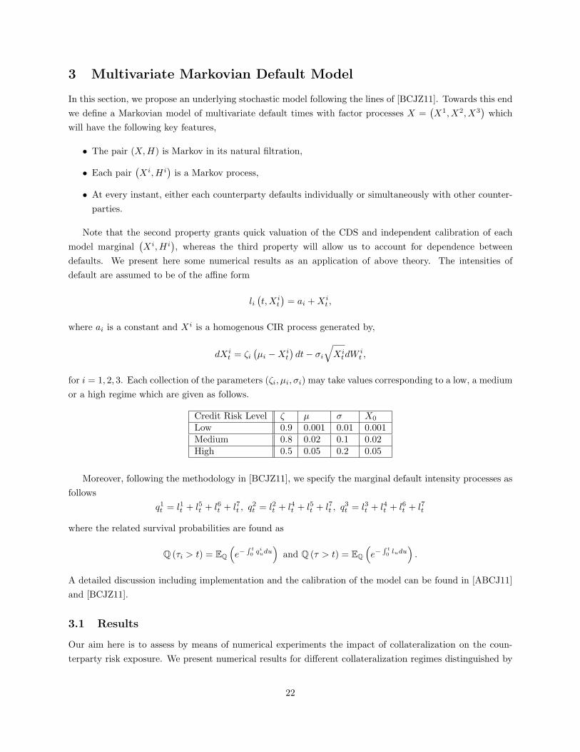
3 Multivariate Markovian Default Model
In this section, we propose an underlying stochastic model following the lines of [BCJZ11]. Towards this end
we define a Markovian model of multivariate default times with factor processes X =(X1, X2, X3
)which
will have the following key features,
• The pair (X,H) is Markov in its natural filtration,
• Each pair(Xi,Hi
)is a Markov process,
• At every instant, either each counterparty defaults individually or simultaneously with other counter-
parties.
Note that the second property grants quick valuation of the CDS and independent calibration of each
model marginal(Xi,Hi
), whereas the third property will allow us to account for dependence between
defaults. We present here some numerical results as an application of above theory. The intensities of
default are assumed to be of the affine form
li(t,Xi
t
)= ai +Xi
t ,
where ai is a constant and Xi is a homogenous CIR process generated by,
dXit = ζi
(µi −Xi
t
)dt− σi
√Xi
tdWit ,
for i = 1, 2, 3. Each collection of the parameters (ζi, µi, σi) may take values corresponding to a low, a medium
or a high regime which are given as follows.
Credit Risk Level ζ µ σ X0
Low 0.9 0.001 0.01 0.001Medium 0.8 0.02 0.1 0.02High 0.5 0.05 0.2 0.05
Moreover, following the methodology in [BCJZ11], we specify the marginal default intensity processes as
follows
q1t = l1t + l5t + l6t + l7t , q2t = l2t + l4t + l5t + l7t , q3t = l3t + l4t + l6t + l7t
where the related survival probabilities are found as
Q (τi > t) = EQ
(e−
∫ t0qiudu
)and Q (τ > t) = EQ
(e−
∫ t0ludu
).
A detailed discussion including implementation and the calibration of the model can be found in [ABCJ11]
and [BCJZ11].
3.1 Results
Our aim here is to assess by means of numerical experiments the impact of collateralization on the coun-
terparty risk exposure. We present numerical results for different collateralization regimes distinguished by
22

different threshold values. The numerical experiments below have been done using the three factor (2F)
parametrization given in [BCJZ11], the recovery rates are fixed to 40%, the risk-free rate r is taken as 0 and
the maturity is set to T = 5 years.
Table 3.1 shows the values of CVA0 and SVA0 for different threshold regimes. Threshold values are
chosen as a fraction of the notional (cf. [Pyk09]). Computations are done assuming that (refer to Table
3) the underlying entity, the counterparty, and the investor has high risk levels. Simulated fair spread
without counterparty risk is found as 153bps. Case A represents the uncollateralized regime where there is
no collateral exchanged (this is done by setting the thresholds infinity), whereas other Case F corresponds
to the full collateralization where the thresholds are set to 0. In each case, computations are done by setting
MTA to zero and assuming there is no margin period. One can observe that decreasing threshold value
dramatically decreases the initial CVA and therefore the SVA values.
Γcpty Γinv CVA0 SVA0
Case A ∞ -∞ 1.0123× 10⁻⁴ 0.2153Case B 1.5× 10⁻³ 0.4× 10⁻³ 6.14× 10⁻⁵ 0.1306Case C 1× 10⁻³ 0.2× 10⁻³ 4.38× 10⁻⁵ 0.0932Case D 0.5× 10⁻³ 0.1× 10⁻³ 2.19× 10⁻⁵ 0.0466Case E 0.25× 10⁻³ 0.05× 10⁻³ 1.16× 10⁻⁵ 0.0247Case F 0 0 0 0
In Figure 1, we present the EPE and ENE curves for each case A to F, and we also plot the mean
collateral values. Computations are carried out by running 104 Monte Carlo simulations. It is apparent that
the behavior of the EPE and ENE values decreases as a result of increased collateralization. Note that
there are peaks in the collateral value in the very beginning and through the maturity. This effect can be
explained as follows: Observe from Table 1 that the investor has lower threshold than the counterparty in
each cases from A to F. As a result, having the lower threshold value, investor will be posting collateral
before the counterparty. Therefore, until the counterparty’s exposure reaches the threshold, the collateral
value remains negative; meaning that there will be margin calls for the investor before the counterparty.
Figure 2 plots the mean of sample CVA paths. Starting from CVA0 we compute the mean sample paths
in each case. The behavior of CVA as a credit hybrid option, as indicated in Remark 2.10, can be clearly
observed in the graphs. CVA values decrease over time as a result of time decay since the expected loss
decreases close to the expiration. The effect of collateralization on the CVA values is apparent in the graphs.
Observe that increased initial threshold values are of great importance since one can significantly reduce the
future CVA values by appropriately setting the collateral thresholds. Moreover, one can also use dynamic
thresholds by linking the threshold values to the counterparties’ default intensities or credit ratings. In
this way, counterparties will have more control on the future values of the CVA of the CDS contract and
dynamically manage the CVA since the collateral thresholds will be reacting to the changes in the default
intensities or credit ratings. This approach will be further investigated in a future research.
4 Conclusion
In this paper, we discussed the modeling of counterparty risk in the presence of bilateral margin agreements.
We defined an appropriate collateral process which takes various margin agreement parameters into account.
The dynamics of the counterparty risk adjustment, CVA, has been found for the bilateral case. This achieve-
23

1 1.5 2 2.5 3 3.5 4 4.5 5
EPEENECollateral
1 1.5 2 2.5 3 3.5 4 4.5 5
EPEENECollateral
1 1.5 2 2.5 3 3.5 4 4.5 5
EPEENECollateral
1 1.5 2 2.5 3 3.5 4 4.5 5
EPEENECollateral
1 1.5 2 2.5 3 3.5 4 4.5 5
EPEENECollateral
1 1.5 2 2.5 3 3.5 4 4.5 5
EPEENECollateral
Figure 1: EPE, ENE and the Collateral curves for Case A, B, C, D, E, and F
ment helps us to better understand and monitor the behavior of the bilateral CVA as well as the unilateral
CVA and the DVA.
We observed the impact of collateral agreements on counterparty risk adjustments as well as the credit
exposures such as the EPE and the ENE. The presence of simultaneous defaults in our model represents
the wrong way risk involved in the CDS contracts. We formulate the fair spread value adjustment, which is
named as SVA, that indicates the additional spread value to incorporate the counterparty risk into the fair
spread value. Moreover, we derive the dynamics of the fair spread and the counterparty risky spread and
therefore the spread value adjustment, SVA. Finally, as in [ABCJ11] and [BCJZ11] we present our numerical
results using a Markovian model of counterparty credit risk.
References
[ABCJ11] S. Assefa, T.R. Bielecki, S. Crepey, and M. Jeanblanc. CVA Computation for Counterparty Risk
Assessment in Credit Portfolios. In Credit Risk Frontiers: Subprime Crisis, Pricing and Hedging,
CVA, MBS, Ratings, and Liquidity. Bloomberg, 2011.
[BC11] T. R. Bielecki and S. Crepey. Dynamic Hedging of Counterparty Exposure. In T. Zariphopoulou,
M. Rutkowski, and Y. Kabanov, editors, The Musiela Festschrift. Spring, 2011.
24

1 1.5 2 2.5 3 3.5 4 4.5 5 1 1.5 2 2.5 3 3.5 4 4.5 5
1 1.5 2 2.5 3 3.5 4 4.5 5 1 1.5 2 2.5 3 3.5 4 4.5 5
1 1.5 2 2.5 3 3.5 4 4.5 5 1 1.5 2 2.5 3 3.5 4 4.5 5
Figure 2: Forward CVA curves for Case A, B, C, D, E, and F
[BCJZ11] T.R. Bielecki, S. Crepey, M. Jeanblanc, and B. Zargari. Valuation and Hedging of CDS Counter-
party Exposure in a Markov Copula Model. Forthcoming in International Journal of Theoretical
and Applied Finance, 2011.
[BJR08] Tomasz R. Bielecki, Monique Jeanblanc, and Marek Rutkowski. Pricing and trading credit default
swaps in a hazard process model. Annals of Applied Probability, 18(6):2495–2529, 2008.
[Gre09] John Gregory. Counterparty Credit Risk: The New Challenge for Global Financial Markets. Wiley,
2009.
[ISD05] ISDA. ISDA Collateral Guidelines. 2005.
[ISD10] ISDA. ISDA Market Review of OTC Derivative Bilateral Collateralization Practices. 2010.
[JLC09] M. Jeanblanc and Y. Le Cam. Immersion property and credit risk modelling. In Optimality and
Risk - Modern Trends in Mathematical Finance, pages 99–132. Springer, 2009.
[Mar09] Markit. The CDS Big Bang: Understanding the Changes to the Global CDS Contract and North
American Conventions. 2009.
[Pyk09] M. Pykhtin. Modeling Credit Exposure for Collateralized Counterparties. Journal of Credit Risk,
5(4):3–27, 2009.
25