Hybrid Control Design for a Wheeled Mobile Robot

Thomas Bak1, Jan Bendtsen1, and Anders P. Ravn2

1 Department of Control Engineering, Aalborg University, Fredrik Bajers Vej 7C, DK-9220Aalborg, Denmark,{tb,dimon}@control.auc.dk

2 Department of Computer Science, Aalborg University, Fredrik Bajers Vej 7E, DK-9220Aalborg, Denmark,apr@cs.auc.dk

Abstract. We present a hybrid systems solution to the problem of trajectorytracking for a four-wheel steered four-wheel driven mobile robot. The robot ismodelled as a non-holonomic dynamic system subject to pure rolling, no-slipconstraints. Under normal driving conditions, a nonlinear trajectory tracking feed-back control law based on dynamic feedback linearization is sufficient to stabilizethe system and ensure asymptotically stable tracking. Transitions to other modesare derived systematically from this model, whenever the configuration space ofthe controlled system has some fundamental singular points. The stability of thehybrid control scheme is finally analyzed using Lyapunov-like arguments.

Keywords: hybrid systems, robot, trajectory tracking, stability analysis

1 Introduction

Wheeled mobile robots is an active research area with promising new application do-mains. Mobile robots are mechanical systems characterized by challenging (noninte-grable) constraints on the velocities which have lead to numerous interesting path track-ing control solutions, [12], [11], [4]. Recently [3] and [1] have addressed the problemfrom a Hybrid systems perspective. We consider a problem of similar complexity anddevelop a systematic approach to derivation of a hybrid automaton and to stability anal-ysis.

Our work is motivated by a project currently in progress, where an autonomousfour-wheel driven, four-wheel steered robot (Figure 1) is being developed. The projectneeds a robot that is able to survey an agricultural field autonomously. The vehiclehas to navigate to certain waypoints where measurements are taken of the crop andweed density. This information is processed and combined to a digital map of the field,which eventually will allow the farm manager to manage weed infestations in a spatiallyprecise manner. The robot is equipped with GPS, gyros, magnetometer and odometers,which will not only help in the exact determination of the location where each imageis taken, but also provide measurements for an estimate of the robot’s position andorientation for a tracking algorithm. Actuation ia achieved using independent steeringand drive motors (8 brushless DC motors in total).

The robot navigates from waypoint to waypoint following spline-type trajectoriesbetween the waypoints to minimize damage to the crop. From a control point of view,this is a tracking problem. To solve this problem we first derived a dynamics model of

Fig. 1. Schematic model of the experimental platform. The robot is equipped with 8 independentsteering and drive motors. Localization is based on fusion of GPS, gyro, magnetometer, andodometer date.

the vehicle subject to pure rolling, no-slip constraints, following the approach taken in[5] and [6].

Next we design a path tracking control law based on feedback linearization. Feed-back linearization designs have the potential of reaching a low degree of conservative-ness, since they rely on explicit cancelling of nonlinearities. However, such designs canalso be quite sensitive to noise, modelling errors, actuator saturation, etc. As pointedout in [8], uncertainties can cause instability under normal driving conditions. This in-stability is caused by loss of invertibility of the mapping representing the nonlinearitiesin the model. Furthermore, there are certain wheel and vehicle velocity configurationsthat lead to similar losses of invertibility. Since these phenomena are, in fact, linked tothe chosen control strategy rather than the mechanics of the robot itself, we propose inthis paper to switch between control strategies such that the aforementioned stabilityissues can be avoided. We intend to motivate the rules for when and how to change be-tween the individual control strategies directly from the mathematical-physical model.We will consider the conditions under which the description may break down duringeach step in the derivation of the model and control laws. These conditions will thendefine transitions in a hybrid automaton that will be used as a control supervisor.

However, introducing a hybrid control scheme in order to improve the operatingrange where the robot can operate in a stable manner comes at a cost: The argumentsfor stability become more complex. Not only must each individual control scheme bestable; they must also be stable under transitions. As one of the main contributions ofthis work, We will therefore apply the generalized Lyapunov stability theory as intro-duced by Branicky in [2].

Even when given suitable Lyapunov functions for each mode, reasoning about over-all stability is still a major effort. We thus abstract the Lyapunov functions to a constantrate function, where the rate is equivalent to the convergence rate. Each mode or state

of the original automaton is then replaced by three consecutive states. The first of thesestates models the initial transition cost and settling period where the function may in-crease, albeit for a bounded time, while the second and third state models the workingmode with the local Lyapunov function. The third state is the transition safe state, wherethe Lyapunov function has decreased below its entry value. All three states are guardedby the original conditions for a mode change; but it is potentially unsafe to leave beforethe third state is entered.

A straightforward analysis will show that the system can always be rendered un-stable: Just vary the reference input such that transitions are always taken before thetransition safe state. We thus add a second automaton constraining the change of thereference input (the trajectory) such that the resulting system remains stable. This au-tomaton defines safe operating conditions, or put another way: Constraints to be satis-fied by the trajectory planner. The composed automaton is in a form, such that it can beanalyzed using model checking tools.

2 Dynamic Model and Linearization

In the following we derive the model and the normal mode control scheme. During thederivation we note conditions for mode changes.

We consider a four-wheel driven, four-wheel steered robot moving on a horizontalplane, constructed from a rigid frame with four identical wheels. Each wheel can turnfreely around its horizontal and vertical axis. The contact points between each of thewheels and the ground must satisfy pure rolling and non-slip conditions.

ICR

Wheel 1

Wheel 2

Wheel 3

Wheel 4

1

M

xv

yv

x

y

-

6

xF

yF

`1γ1

θ

Fig. 2. Definition of the field coordinate system(xF , yF ), vehicle coordinate system(xv, yv),vehicle orientationθ, distance 1, and directionγ1 from the center of mass(x, y) to wheel 1.Each wheel plane is perpendicular to the Instantaneous Center of Rotation (ICR).

Consider a reference (‘field’) coordinate system(xF , yF ) in the plane of motion asillustrated in Figure 2. The robot position is then completely described by the coordi-nates(x, y) of a reference point within the robot frame, which without loss of generality

can be chosen as the center of mass, and the orientationθ relative to the field coordi-nate system of a (‘vehicle’) coordinate system(xv, yv) fixed to the robot frame. Thesecoordinates are collected in theposturevectorξ = [x y θ]T ∈ R2 × S1.

The position of thei’th wheel (1 ≤ i ≤ 4) in the vehicle coordinate system ischaracterized by the angleγi and the distancei.

As the wheels are not allowed to slip, the planes of each of the wheels must at alltimes be tangential to concentric circles with the center in the Instantaneous Center ofRotation (ICR). The orientation of the plane of thei’th wheel relative toxv is denotedβi. The vectorβ = [β1 β2 β3 β4]T ∈ S4 define the wheel orientations.

From an operational point of view a relevant specification of the ICR is to give theorientation of two of the four wheels. We therefore partitionβ into βc ∈ S2 contain-ing the coordinates used to control the ICR location andβo ∈ S2 containing the tworemaining coordinates that may be derived from the first.

Cross Driving (Singular Wheel Configuration) An important ambiguity (or singularwheel configuration), is present in the approach taken above. Forβ1 = ±π/2 andβ2 =±π/2 the configuration of wheels 3 and 4 is not defined. The situation corresponds tothe ICR being located on the line through wheel 1 and 2. The wheel configurationβc =[β3 β4]T result in similar problems and both configurations fail during cross driving asall wheels are at±π/2 i.e. ICR at infinity (andθ = 0). To ensure safe solutions to thetrajectory tracking problem we must ensure that the singular configurations are avoidedat all times. Based on this discussion we identify three discrete control modes,q1, q2

andq3:

q1: Trajectory tracking withβc = [β1 β2]T. This mode is conditioned on|β1| < (π/2−b) ∧ |β2| < (π/2− b) ∧ |θ| ≥ o.

q2: Trajectory tracking withβc = [β3 β4]T. This mode is conditioned on|β3| < (π/2−b) ∧ |β4| < (π/2− b) ∧ |θ| ≥ o.

q3: Cross Driving withβ1 = β2 = β3 = β4. This mode is conditioned on|θ| < o.

whereb and o are small positive numbers. The two first modes cover the situationswhere the ICR is governed by wheels 1 and 2 and by wheel 3 and 4, respectively, whilethe latter covers the situation where the ICR is at infinity. For brevity of the exposition,we will considerβc = [β1 β2]T in the following; the case withβc = [β3 β4]T isanalogous.

As presented here, the problem is specific to the proposed representation of theICR, but in general, no set of two variables is able to describe all wheel configurationswithout singularities [13]. That is, the problem of such singular configurations is notdue to the representation used, but is a general problem for this type of robotic systems.

2.1 Vehicle Model

Following the argumentation in Appendix A, robot posture can be manipulated via onevelocity inputη(t) ∈ R in the instantaneous direction ofΣ(βc) ∈ R3 which is con-structed to meet the pure-roll constraint. Similarly, it is possible to manipulate the ori-entations of the wheels via an orientation velocity inputζ(t) = [β1 β2]T ∈ R2. The

no-slip condition on the wheels that constrainη(t) is handled (see Appendix A) by ap-plying Lagrange formalism and computed torque techniques. The result is the followingextended dynamical model:

χ =

ξη

βc

=

0 RT(θ)Σ(βc) 00 0 00 0 0

χ +

0 01 00 I

[νζ

](1)

whereν is a new exogenous input that is related to the torque applied to the drivemotors. In equation (1) it is assumed that theβ dynamics can be controlled via localservo loops, such that we can manipulateβ as an exogenous input to the model.

2.2 Normal Trajectory Tracking Control

Provided that we avoid the singular wheel configurations the standard approach fromhere on is to transform the states into normal form via an appropriate diffeomorphismfollowed by feedback linearization of the nonlinearities and a standard linear controldesign. We choose the new states

x1 = T (χ) =[ξref − ξ

ξref − ξ

], (2)

which yields the following dynamics:

x1 = A1x1 + B1

(δ(χ)

[νζ

]− α(χ)

), A1 =

[0 I0 0

], B1 =

[0I

]. (3)

Using the results from Appendix A,δ(χ) andα(χ) may be found to

δ(χ) = RT(θ)[Σ(βc) N(βc)η

](4)

and

α(χ) = sin(β1 − β2)η2

−`1 sin β2 cos(β1 − γ1) + `2 sin β1 sin(β2 − γ2)`1 cosβ2 cos(β1 − γ1)− `2 cosβ1 cos(β2 − γ2)

0

(5)

whereN(βc) = [N1 N2] is specified in equations (19) and (20). If we then apply thecontrol law [

νζ

]= δ(χ)−1(α(χ)−K1x1) (6)

we obtain the closed-loop dynamicsx1 = (A1−B1K1)x1, which tends to0 ast →∞if K1 is chosen such thatA1 − B1K1 has eigenvalues with negative real parts. Similardynamics can be obtained for the situation withβc = [β3 β4]T, resulting in closed-loopdynamicsx2 = (A2 −B2K2)x2.

2.3 Parallel Wheels Control

Due to the conditions imposed on the trajectory tracking controllers, an additional con-trol scheme must be derived that is able to control the vehicle when all four wheels areparallel, which forcesθ to 0. Fortunately, the dynamics of the robot becomes particu-larly simple in this case.

With θ = 0 the dynamics are immediately linear; hence, choosing the states

x3 = Tχ =[ξref − ξ

ξref − ξ

], (7)

whereT is an appropriate invertible matrix, then yields the dynamics

x3 = A3x3 + B3

[ν0

], A3 =

[0 I

A31 A32

], B3 =

[0I

](8)

which can be controlled by applying the feedbackν = −K3x3.

Rest Configurations

During the feedback linearization design we detect another interesting condition dueto the inversion ofδ(χ). If δ(χ) looses rank, the control strategy breaks down and thecontrol input grows to infinity. If we avoid the rest configuration,η = 0, thenΣ(βc)specifies the current direction of movement and the column vectorsN1 and N2 areperpendicular to this direction and to each other. To avoid an ill-conditionedδ(χ) wemust impose a new condition,|η| ≥ n, wheren is a small positive number, on ourtrajectory tracking modes,q1 andq2.

To complete the construction, we add additional modes to handle the rest configu-ration. First assume that the robot is started withβ1 = β2 = β3 = β4. We may thenutilize the controller defined for theq3 mode, choosingξref as an appropriate point onthe straight line originating from the center of mass in the direction defined byβ alongwith

ξref =[ηref

ζref

]=

[2n0

]

This mode would allow the robot to start from rest and adds a mode (q0). Finally weadd a modeq4 to handle the stop situation. Again we assume that the wheels have beenoriented by the control laws in modeq1 or q2 such that the waypoint lies on the straightline from the center of mass in the direction defined byβ. We may then apply the samestate transformation as in (7) along with the same state feedback, and choosingξref

as the target waypoint along withξref = 0. As a result|η| ≥ n is added to the modeconditions forq1, q2, and two new modesq0 andq4 are added to handle the start fromrest and the stop situations respectively.

3 Hybrid Automaton Supervisor

The trajectory tracking problem for this particular robot may be solved by applying thedifferent control laws, as outlined above for different modes. The conditions for exiting

the modes have been defined as well. For each of these modes, we defined specialcontrol schemes, and conditions. Given that there are two modes where the robot is atrest, and three modes where the robot is driving, it is straightforward to introduce twosuper-modes,RestandDriving. This gives rise to the hierarchical hybrid automatonimplemented using Stateflow as shown in Figure 3.

DrivingRest

q0_start

q1_left_wheels

q2_right_wheels

q3_parallel_wheels

q4_stop

/mode=Q4[abs_beta[1]<BLIM & abs_beta[2]<BLIM & abs_bdot >= o]/mode=Q1

[abs_eta<=ELIM]

[abs_beta[3]<BLIM & abs_beta[4]<BLIM & abs_bdot >= o]/mode=Q2

[abs_beta[1]<BLIM & abs_beta[2]<BLIM & abs_bdot >= o]/mode=Q1

[abs_bdot<o]/mode=Q3

[new_wp==1]/mode=Q0

[abs_bdot<o]/mode=Q3

[abs_beta[3]<BLIM & abs_beta[4]<BLIM & abs_bdot >= o]/mode=Q2

[abs_eta>ELIM]

/mode=Q3

Fig. 3. Stateflow representation of Automaton.

The hybrid automaton [10] consists of five discrete states,Q = {q0, q1, q2, q3, q4}as defined during the model and controller derivation.

The continuous statex defined by equation (2) or (7) belongs to the state spaceX ⊆ R2 × S1 × R3. The corresponding hybrid state space isH = Q×X. The vectorfields are defined by

f(q, x) =

(A3 −B3K3)x0 if q = q0,

(A1 −B1K1)x1 if q = q1,

(A2 −B2K2)x2 if q = q2,

(A3 −B3K3)x3 if q = q3,

(A3 −B3K3)x4 if q = q4.

(9)

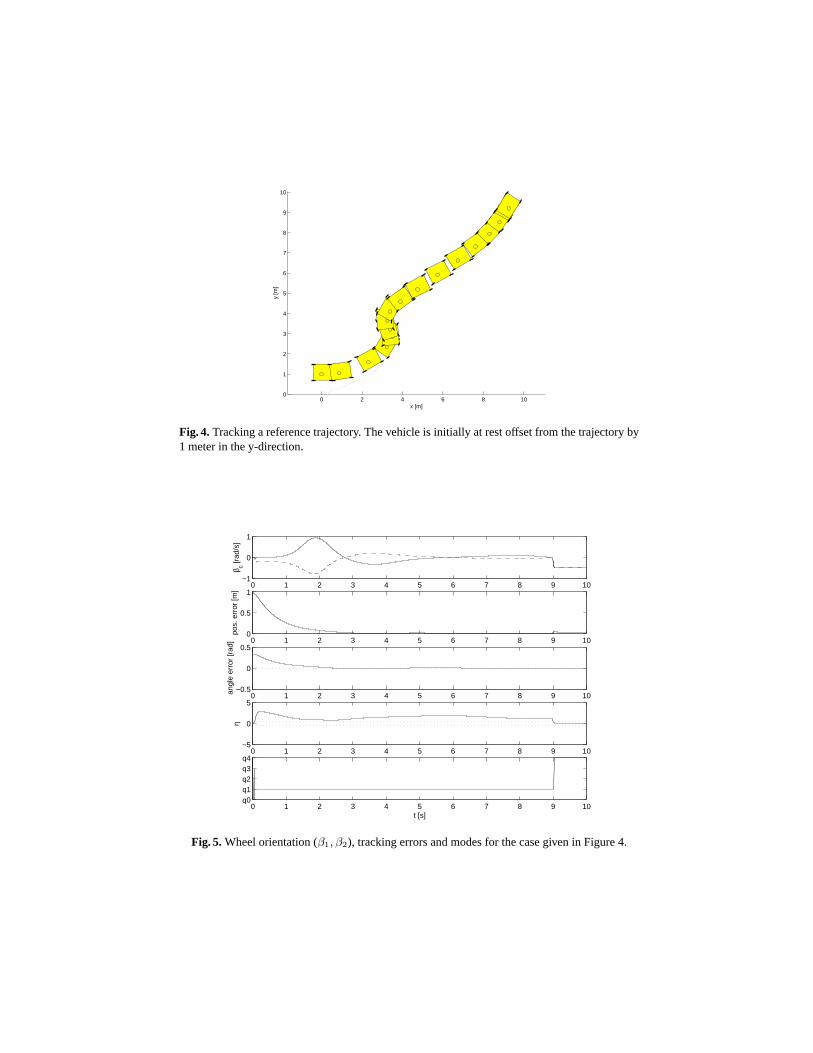
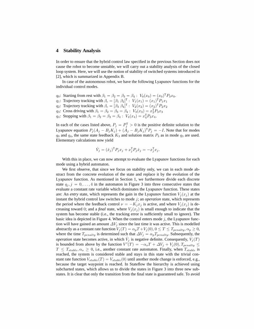
Conditions and guards are given in Figure 3 based on the derivations in Section 2.The system including the supervisor was simulated in Simulink and the tracking of anexample trajectory is shown in Figure 4. The system is clearly able to start from an restconfiguration, track the trajectory and stop at a rest configuration. In this example thecontroller starts in the modeq4, switches to a new waypoint and trajectory informationbecomes available. Asη grows the mode is changed toq3 and eventuallyq1 where itremains until the vehicle returns toq4 and stops. Mode changes, tracking errors andwheel positions are given in Figure 5.

0 2 4 6 8 100

1

2

3

4

5

6

7

8

9

10

x [m]

y [m

]

Fig. 4.Tracking a reference trajectory. The vehicle is initially at rest offset from the trajectory by1 meter in the y-direction.

0 1 2 3 4 5 6 7 8 9 10−1

0

1

β c [rad

/s]

0 1 2 3 4 5 6 7 8 9 100

0.5

1

pos.

err

or [m

]

0 1 2 3 4 5 6 7 8 9 10−0.5

0

0.5

angl

e er

ror

[rad

]

0 1 2 3 4 5 6 7 8 9 10−5

0

5

η

0 1 2 3 4 5 6 7 8 9 10q0q1q2q3q4

t [s]

Fig. 5. Wheel orientation (β1, β2), tracking errors and modes for the case given in Figure 4.

4 Stability Analysis

In order to ensure that the hybrid control law specified in the previous Section does notcause the robot to become unstable, we will carry out a stability analysis of the closedloop system. Here, we will use the notion of stability of switched systems introduced in[2], which is summarized in Appendix B.

In case of the autonomous robot, we have the following Lyapunov functions for theindividual control modes.

q0: Starting from rest withβ1 = β2 = β3 = β4 : V0(x0) = (x0)TP3x0.q1: Trajectory tracking withβc = [β1 β2]T : V1(x1) = (x1)TP1x1

q2: Trajectory tracking withβc = [β3 β4]T : V2(x2) = (x2)TP2x2

q3: Cross driving withβ1 = β2 = β3 = β4 : V3(x3) = xT3P3x3

q4: Stopping withβ1 = β2 = β3 = β4 : V4(x4) = xT4P3x4.

In each of the cases listed above,Pj = P Tj > 0 is the positive definite solution to the

Lyapunov equationPj(Aj − BjKj) + (Aj − BjKj)TPj = −I. Note that for modesq0 andq4, the same state feedbackK3 and solution matrixP3 as in modeq3 are used.Elementary calculations now yield

Vj = (xj)TPjxj + xTj Pj xj = −xT

j xj .

With this in place, we can now attempt to evaluate the Lyapunov functions for eachmode using a hybrid automaton.

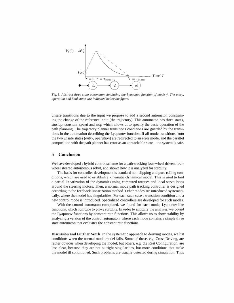
We first observe, that since we focus on stability only, we can in each mode ab-stract from the concrete evolution of the state and replace it by the evolution of theLyapunov function. As mentioned in Section 1, we furthermore divide each discretestateqj , j = 0, . . . , 4 in the automaton in Figure 3 into three consecutive states thatevaluate a constant rate variable which dominates the Lyapunov function. These statesare: Anentry state, which represents the gain in the Lyapunov functionVj(xj) at theinstant the hybrid control law switches to modej; anoperationstate, which representsthe period where the feedback controlν = −Kjxj is active, and whereVj(xj) is de-creasing toward0; and afinal state, whereVj(xj) is small enough to indicate that thesystem has become stable (i.e., the tracking error is sufficiently small to ignore). Thebasic idea is depicted in Figure 4. When the control enters modej, the Lyapunov func-tion will have gained an amount∆Vj since the last time it was active. This is modelledabstractly as a constant rate functionVj(T ) = αpT +Vj(0), 0 ≤ T ≤ Tpenalty, αp ≥ 0,where the timeTpenalty is determined such that∆Vj = αpTpenalty. Subsequently, theoperationstate becomes active, in whichVj is negative definite. Consequently,Vj(T )is bounded from above by the functionV ′(T ) = −αoT + ∆Vj + Vj(0), Tpenalty ≤T ≤ Tstable, αo ≥ 0, i.e., another constant rate automaton. Finally, whenTstable isreached, the system is considered stable and stays in this state with the trivial con-stant rate functionVstable(T ) = Vstable(0) until another mode change is enforced, e.g.,because the target waypoint is reached. In Stateflow the hierarchy is achieved usingsubcharted states, which allows us to divide the states in Figure 3 into three new sub-states. It is clear that only the transition from the final state is guaranteed safe. To avoid

-

6Vj(0) + ∆Vj

Vj(0)’Time’ T

T = 0 T = Tpenalty T = Tstable

- q′0 - q′1 - q′2

Fig. 6. Abstract three-state automaton simulating the Lyapunov function of modej. The entry,operation and final states are indicated below the figure.

unsafe transitions due to the input we propose to add a second automaton constrain-ing the change of the reference input (the trajectory). This automaton has three states,startup, constant_speedandstopwhich allows ut to specify the basic operation of thepath planning. The trajectory planner transitions conditions are guarded by the transi-tions in the automation describing the Lyapunov function. If all mode transitions fromthe two unsafe states (entry, operation) are redirected to an error mode, and the parallelcomposition with the path planner has error as an unreachable state – the system is safe.

5 Conclusion

We have developed a hybrid control scheme for a path-tracking four-wheel driven, four-wheel steered autonomous robot, and shown how it is analyzed for stability.

The basis for controller development is standard non-slipping and pure rolling con-ditions, which are used to establish a kinematic-dynamical model. This is used to finda partial linearization of the dynamics using computed torques and local servo loopsaround the steering motors. Then, a normal mode path tracking controller is designedaccording to the feedback linearization method. Other modes are introduced systemati-cally, where the model has singularities. For each such case a transition condition and anew control mode is introduced. Specialized controllers are developed for such modes.

With the control automaton completed, we found for each mode, Lyaponov-likefunctions, which combine to prove stability. In order to simplify the analysis, we boundthe Lyapunov functions by constant rate functions. This allows us to show stability byanalyzing a version of the control automaton, where each mode contains a simple threestate automaton that evaluates the constant rate functions.

Discussion and Further Work In the systematic approach to deriving modes, we listconditions when the normal mode model fails. Some of these, e.g. Cross Driving, arerather obvious when developing the model; but others, e.g. the Rest Configuration, areless clear, because they are not outright singularities, but more conditions that makethe model ill conditioned. Such problems are usually detected during simulation. Thus

a practical rendering of the systematic approach is to use a tool like Stateflow andbuild the normal mode model. When the simulation has problems, one investigates theconditions and defines corresponding transitions. An approach that we believe is widelyapplicable to design of supervisory or mode switched control systems.

Such a divide and conquer approach is evidently only safe to the extent that it isfollowed by a rigorous stability analysis.The approach which we develop is very sys-tematic. It ends up with a constant rate hybrid automaton which should allow modelchecking of its properties. In particular, whether it avoids unsafe transitions when com-posed with an automaton modelling the reference input. A systematic analysis of thiscombination is, however, future work.

Another point that must be investigated is, how the wheel reference output is madebumpless during mode transitions.

References

1. C. Altafini, A. Speranzon, K.H. Johansson. Hybrid Control of a Truck and Trailer Vehicle, InC. Tomlin, and M. R. Greenstreet, editors,Hybrid Systems: Computation and ControlLNCS2289, p. 21ff, Springer-Verlag, 2002.

2. M. S. Branicky. Analyzing and Synthesizing Hybrid Control Systems In G. Rozenberg, andF. Vaandrager, editors,Lectures on Embedded Systems, LNCS 1494, pp. 74-113, Springer-Verlag, 1998.

3. A. Balluchi, P. Souères, and A. Bicchi. Hybrid Feedback Control for Path Tracking by aBounded-Curvature Vehicle In M.D. Di Benedetto, and A.L. Sangiovanni-Vincentelli, editors,Hybrid Systems: Computation and Control, LNCS 2034, pp. 133–146, Springer-Verlag, 2001.

4. G. Bastin, G. Campion. Feedback Control of Nonholonomic Mechanical Systems,Advancesin Robot Control, 1991

5. B. D’Andrea-Novel, G. Campion, G. Bastin. “Modeling and Control of Non HolonomicWheeled Mobile Robots, inProc. of the 1991 IEEE International Conference on Roboticsand Automation, 1130–1135, 1991

6. G. Campion, G. Bastin, B. D’Andrea-Novel. “Structural Properties and Classification of Kine-matic and Dynamic Models of Wheeled Mobile Robots,IEEE Transactions on Robotics andAutomationVol. 12, 1:47-62, 1996

7. L. Caracciolo, A. de Luca, S. Iannitti. “Trajectory Tracking of a Four-Wheel DifferentiallyDriven Mobile Robot, inProc. of the 1999 IEEE International Conference on Robotics andAutomation, 2632–2838, 1999

8. J.D. Bendtsen, P. Andersen, T.S. Pedersen. “Robust Feedback Linearization-based ControlDesign for a Wheeled Mobile Robot, inProc. of the 6th International Symposium on AdvancedVehicle Control, 2002

9. H. Goldstein. Classical Mechanics, Addison-Wesley, 2nd edition, 198010. T. A. Henzinger. The Theory of Hybrid Automata„ InProceedings of the 11th Annual IEEE

Symposium on Logic in Computer Science(LICS 1996), pp. 278-292, 1996.11. C. Samson. Feedback Stabilization of a Nonholonomic Car-like Mobile Robot, InProceed-

ings of IEEE Conference on Decision and Control, 1991.12. G. Walsh, D. Tilbury, S. Sastry, R. Murray, J.P. Laumond. Stabilization of Trajectories for

Systems with Nonholonomic Constraints IEEE Trans. Automatic Control, 39: (1) 216-222,1994

13. B. Thuilot, B. D’Andrea-Novel, A. Micaelli. “Modeling and Feedback Control of MobileRobots Equipped with Several Steering Wheels,IEEE Transactions on Robotics and Automa-tion Vol. 12, 2:375-391, 1996

A Vehicle Dynamics

Denote the rotation coordinates describing the rotation of the wheels around their hor-izontal axes byφ = [φ1 φ2 φ3 φ4]T ∈ S4 and the radii of the wheels byr =[r1 r2 r3 r4] ∈ R4. The motion of the four-wheel driven, four-wheel steered robotis then completely described by the following 11 generalized coordinates:

q =[x y θ βT φT

]T =[ξT βT φT

]T(10)

and we can write the pure rolling, no slip constraints on the compact matrix form

A(q)q =[J1(β)R(θ) 0 J2

C1(β)R(θ) 0 0

]q = 0 (11)

in which

J1(β) =

cos β1 sin β1 `1 sin(β1 − γ1)cos β2 sin β2 `2 sin(β2 − γ2)cos β3 sin β3 `3 sin(β3 − γ3)cos β4 sin β4 `4 sin(β4 − γ4)

, J2 = rI4×4,

C1(β) =

− sin β1 cosβ1 `1 cos(β1 − γ1)− sin β2 cosβ2 `2 cos(β2 − γ2)− sin β3 cosβ3 `3 cos(β3 − γ3)− sin β4 cosβ4 `4 cos(β4 − γ4)

, andR(θ) =

cos θ sin θ 0− sin θ cos θ 0

0 0 1

.

Following the argumentation in [6], the posture velocityξ is constrained to belongto a one-dimensional distribution here parametrized by the orientation angles of twowheels, say,β1 andβ2. Thus,

ξ ∈ span{col{R(θ)TΣ(βc)}}whereΣ(βc) ∈ R3 is perpendicular to the space spanned by the columns ofC1, i.e.,C1(β)Σ(βc) ≡ 0 ∀β. Σ can be found by combining the expression forC1(β) withequations for the orientation of wheels 3 and 4 to

Σ =

`1 cosβ2 cos(β1 − γ1)− `2 cos β1 cos(β2 − γ2)`1 sin β2 cos(β1 − γ1)− `2 sin β1 cos(β2 − γ2)

sin(β1 − β2)

.

The discussion above implies that the robot posture can be manipulated via onevelocity inputη(t) ∈ R in the instantaneous direction ofΣ(βc), that is,R(θ)ξ(t) =Σ(βc)η(t) ∀t. Similarly, it is possible to manipulate the orientations of the wheels viaan orientation velocity inputζ(t) = [β1 β2]T ∈ R2.

The constrained dynamics ofη are handled by applying Lagrange formalism andcomputed torque techniques as suggested in [5] and [6].

The Lagrange equations for non-holonomic systems are written on the form [9]

d

dt

(∂T

∂qk

)− ∂T

∂qk= ck(q)Tλ + Qk

in whichT is the total kinetic energy of the system andqk is thek’th generalized coor-dinate. On the left-hand side,ck(q) is thek’th column in the kinematic constraint matrixA(q) defined in (11),λ is a vector of so-calledLagrange undetermined coefficients, andQk is a generalized force (or torque) acting on thek’th generalized coordinate.

The kinetic energy of the robot is calculated as

T =12qT

R(θ)TMR(θ) R(θ)TV 0V TR(θ) Jβ 0

0 0 Jφ

q (12)

with appropriate choices ofM , Jβ andJφ. In the case of the wheeled mobile robot wecan derive the following expressions:

M =

mf + 4mw 0 −mw

∑4i=1 `i sin γi

0 mf + 4mw mw

∑4i=1 `i cos γi

−mw

∑4i=1 `i sin γi mw

∑4i=1 `i cos γi If + mw

∑4i=1 γ2

i

. (13)

Here,If is the moment of inertia of the frame around the center of mass, andmf andmw are the masses of the robot frame and each wheel, respectively. We note that sincethe wheels are placed symmetrically around thexv andyv axes, the off-diagonal termsshould vanish. However, this may not be possible to achieve completely in practice, dueto uneven distribution of equipment within the robot.

Turning to the wheels, we denote the moment of inertia of each wheel byIw andfind

Jβ =12IwI4×4 and Jφ = IwI4×4 (14)

and

V =

0 0 0 00 0 0 0Iw Iw Iw Iw

. (15)

The Lagrange undetermined coefficients are then eliminated in order to arrive at thefollowing dynamics:

h1(β)η + Φ1(β)ζη = ΣTEτφ (16)

in which E = JT1 J−1

2 ∈ R3×4 andτφ ∈ R4 is a vector of torques applied to drive thewheels. The quadratic functionh1(β) is given by

h1(β) = ΣT(M + EJφET)Σ > 0 (17)

andΦ1(β) ∈ R is given by

Φ1(β) = ΣT(M + EJφET)N(βc) (18)

N(βc) = [N1 N2], where

N1 =

−`1 cos β2 sin(β1 − γ1) + `2 sin β1 cos(β2 − γ2)−`1 sin β2 sin(β1 − γ1)− `2 cosβ1 cos(β2 − γ2)

cos(β1 − β2)

(19)

N2 =

−`1 sin β2 cos(β1 − γ1) + `2 cos β1 sin(β2 − γ2)`1 cosβ2 cos(β1 − γ1) + `2 sinβ1 sin(β2 − γ2)

− cos(β1 − β2)

(20)

Equation (16) can be linearized by using a computed torque approach and choosingτφ

appropriately. The torques are simply distributed evenly to each wheel; we observe that

ΣTEτφ = [a1 a2 a3 a4]

τ1

τ2

τ3

τ4

= L

whereL is the left-hand side of (16). Then we setτφ = Hτ0, H ∈ R4 and chooseHi = Lsign(ai)/σ, whereσ is the sum of the four entries in the vectorΣTE. Thisdistribution policy ensures that the largest torque applied to the individual wheels is assmall as possible.

Hence, by applying the torque

τ0 =1

ΣTEH(h1(β)ν + Φ1(β)ζη) , (21)

we obtainη = ν

whereν is a new exogenous input. The result of the extension and partial linearizationis the dynamical model given in Equation 1.

B Stability of Switched Systems

Consider a dynamic system whose behavior at any given timet ≥ t0, wheret0 is anappropriate initial time, is described by one out of several possible individual sets ofcontinuous-time differential equationsΣ0, Σ1, . . . , Σµ, and letx0(t), x1(t), . . . , xµ(t)denote the corresponding state vectors for the individual systems:

Σj : xj = fj(xj(t)), j = 0, 1, . . . , µ

The governing set of differential equations is switched at discrete instancesti, i =0, 1, 2, . . . ordered such thatti < ti+1∀i. That is, the system behavior is governed byΣj in the time intervalti < t ≤ ti+1, then byΣk in the time intervalti+1 < t ≤ ti+2,and so forth. Assume furthermore that for eachΣj there exists a Lyapunov function,i.e., a scalar functionVj(xj(t)) satisfyingVj(0) = 0, Vj(xj) ≥ 0, andV (xj) ≤ 0 forxj 6= 0. It is noted that, by the last requirement,Vj is a non-increasing function of timein the interval whereΣj is active. Hence, it can be deduced that the switched systemgoverned by the sequence of sets of differential equations is stable if it can be shownthat

Vj(xj(tq)) ≥ Vj(xj(tr))

for all 0 ≤ j ≤ µ andtq, tr ∈ {ti}, wheretq < tr are the last and current switchingtime whereΣj became active, respectively.