modeling and control of a hybrid wheeled legged robot
TRANSCRIPT

Modeling and Control of a Hybrid Wheeled LeggedRobot: Disturbance AnalysisFahad Raza ( [email protected] )
Tohoku University https://orcid.org/0000-0003-4798-2358Dai Owaki
Tohoku DaigakuMitsuhiro Hayashibe
Tohoku Daigaku
Research Article
Keywords: Balance Control, Wheel-legged Robots, Optimal Control, Self-balancing Robot
Posted Date: February 6th, 2020
DOI: https://doi.org/10.21203/rs.2.22794/v1
License: This work is licensed under a Creative Commons Attribution 4.0 International License. Read Full License

1
Modeling and Control of a Hybrid Wheeled Legged Robot: Disturbance Analysis
Fahad Raza, Dai Owaki, and Mitsuhiro Hayashibe Senior Member, IEEE
Abstract—The most common cause of injuries among olderadults is falling. Recently, there have been numerous develop-ments in assistive and exoskeleton systems. However, compara-tively little work is being done on systems that may help peopleto keep an upright position and avoid falling over. In this prelimi-nary work, we investigate the feasibility of the wheel-legged robotas a balance-assist system for the people who cannot maintainbalance and walk because of an injury, old age, or neurologicalor physical disorder. We perform motion stability analyses ofthe wheel-legged robot under different conditions such as systemmodeling errors, sensor noise, and external disturbances. Thelinear quadratic regulator (LQR) control approach is adoptedfor balancing, steering, and translational position control of therobot. To validate our control framework and visualize results,the robot is modeled and tested in the Gazebo simulator usingROS (Robot Operating System). Subsequently, the simulationresults demonstrate the effectiveness of the LQR control methodunder the translational and rotational pushes of the wheel-leggedsystem for human-robot interaction.
Index Terms—Balance Control, Wheel-legged Robots, OptimalControl, Self-balancing Robot.
I. INTRODUCTION
The most common cause of injuries among older adults is
falling [1]. These injuries not only affect the physical health
of patients but also place an appreciable financial burden on
governmental healthcare budgets. Fall-induced injuries are a
major source of longstanding pain, physical disability, and
death among older adults [2].
In recent years, numerous performance-augmenting and
rehabilitation exoskeleton systems have been developed by
robotics companies and researchers for able-bodied people and
physically disabled patients, respectively [3]. As an example,
a leg exoskeleton developed for able-bodied people provides
positive mechanical power to the ankle during push-off [4].
Ma et. al. designed a wheeled-foot exoskeleton for paraplegic
patients, allowing users to walk with a standing posture [5].
An assistive intelligent walker is developed to help the elderly,
handicapped, or blind people by employing servo brakes [6]. A
team from UC Berkeley developed a lower-extremity exoskele-
ton called BLEEX (Berkeley Lower Extremity Exoskeleton)
[7]. It is the first field-operational exoskeleton that helps users
carry an appreciable load with minimal effort.
As illustrated by the above mentioned works, there has been
vast interest in developing robotic systems for performance
augmentation, and the rehabilitation of people. However to the
best of the authors’ knowledge, there has been comparatively
F. Raza and D. Owaki are with the Department of Robotics, Grad-uate School of Engineering, Tohoku University, Sendai 980-8579, Japan(email: [email protected]; [email protected]).
M. Hayashibe is concurrently with the Graduate School of BiomedicalEngineering and the Department of Robotics, Graduate School of Engineering,Tohoku University, Sendai 980-8579, Japan (email: [email protected]).
(a) Front View. (b) Side View.
Fig. 1: Wheel-legged robot in the Gazebo simulator.
little work on developing systems that may help people to
keep an upright position and avoid falling over. A rather rare
example of the balance-assist systems is a lower body ex-
oskeleton that consists of powered hip flexion/extension (HFE)
and hip abduction/adduction (HAA) joints to support walking
and balancing [8]. We therefore investigate the feasibility of
a wheel-legged biped robot that helps prevent older adults
and paraplegic patients from falling. Adaptability to various
terrain is of critical importance to human-assistance robotic
systems, as users live in different environments. We know
that legged locomotion is robust in terms of climbing stairs
and traversing rough terrain, whereas wheel mechanisms are
energy efficient for traversing flat terrain. A hybrid wheel-
legged robotic system has the advantages of both leg and wheel
mechanisms, and it adapts its locomotion to the requirements
of given terrain. Moreover, a biped wheel-legged system
provides the complex balancing reactions needed to keep the
center of mass (CoM) within the base of support of a human
body.
Wheel-legged systems have recently caught the attraction
of the search and rescue, rapid exploration, and logistics
robotics community; a fascinating example of such systems
is a wheeled biped robot called Handle manufactured by the
Boston Dynamics [9]. While Handle has shown remarkable
balancing and manipulation feats, yet its locomotion and
control frameworks have not been shared with the open
research community. Another two-wheeled human assistant
robot with sitting and running capabilities was proposed by
[10]. To take the advantage of both wheeled and legged
locomotion, a small wheel-legged robot PAW is presented
by [11]. They designed the robot in such a way that its
legs are capable of limited recirculation helping it to gain
a cruise speed of up to 2 m/s. Suzumura et. al. modeled a
quadruped wheel-legged mobile robot in three dimensions and
2
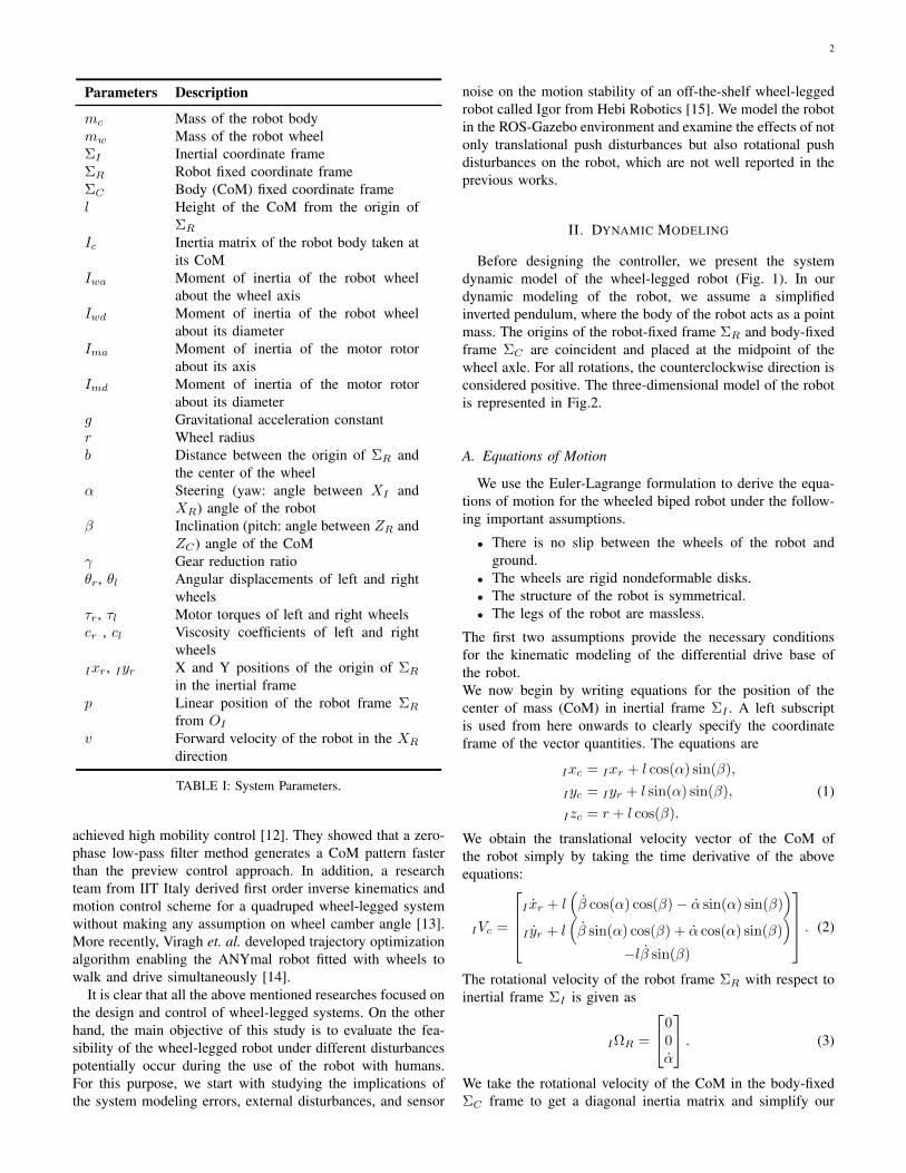
Parameters Description
mc Mass of the robot body
mw Mass of the robot wheel
ΣI Inertial coordinate frame
ΣR Robot fixed coordinate frame
ΣC Body (CoM) fixed coordinate frame
l Height of the CoM from the origin of
ΣR
Ic Inertia matrix of the robot body taken at
its CoM
Iwa Moment of inertia of the robot wheel
about the wheel axis
Iwd Moment of inertia of the robot wheel
about its diameter
Ima Moment of inertia of the motor rotor
about its axis
Imd Moment of inertia of the motor rotor
about its diameter
g Gravitational acceleration constant
r Wheel radius
b Distance between the origin of ΣR and
the center of the wheel
α Steering (yaw: angle between XI and
XR) angle of the robot
β Inclination (pitch: angle between ZR and
ZC) angle of the CoM
γ Gear reduction ratio
θr, θl Angular displacements of left and right
wheels
τr, τl Motor torques of left and right wheels
cr , cl Viscosity coefficients of left and right
wheels
Ixr, Iyr X and Y positions of the origin of ΣR
in the inertial frame
p Linear position of the robot frame ΣR
from OI
v Forward velocity of the robot in the XR
direction
TABLE I: System Parameters.
achieved high mobility control [12]. They showed that a zero-
phase low-pass filter method generates a CoM pattern faster
than the preview control approach. In addition, a research
team from IIT Italy derived first order inverse kinematics and
motion control scheme for a quadruped wheel-legged system
without making any assumption on wheel camber angle [13].
More recently, Viragh et. al. developed trajectory optimization
algorithm enabling the ANYmal robot fitted with wheels to
walk and drive simultaneously [14].
It is clear that all the above mentioned researches focused on
the design and control of wheel-legged systems. On the other
hand, the main objective of this study is to evaluate the fea-
sibility of the wheel-legged robot under different disturbances
potentially occur during the use of the robot with humans.
For this purpose, we start with studying the implications of
the system modeling errors, external disturbances, and sensor
noise on the motion stability of an off-the-shelf wheel-legged
robot called Igor from Hebi Robotics [15]. We model the robot
in the ROS-Gazebo environment and examine the effects of not
only translational push disturbances but also rotational push
disturbances on the robot, which are not well reported in the
previous works.
II. DYNAMIC MODELING
Before designing the controller, we present the system
dynamic model of the wheel-legged robot (Fig. 1). In our
dynamic modeling of the robot, we assume a simplified
inverted pendulum, where the body of the robot acts as a point
mass. The origins of the robot-fixed frame ΣR and body-fixed
frame ΣC are coincident and placed at the midpoint of the
wheel axle. For all rotations, the counterclockwise direction is
considered positive. The three-dimensional model of the robot
is represented in Fig.2.
A. Equations of Motion
We use the Euler-Lagrange formulation to derive the equa-
tions of motion for the wheeled biped robot under the follow-
ing important assumptions.
• There is no slip between the wheels of the robot and
ground.
• The wheels are rigid nondeformable disks.
• The structure of the robot is symmetrical.
• The legs of the robot are massless.
The first two assumptions provide the necessary conditions
for the kinematic modeling of the differential drive base of
the robot.
We now begin by writing equations for the position of the
center of mass (CoM) in inertial frame ΣI . A left subscript
is used from here onwards to clearly specify the coordinate
frame of the vector quantities. The equations are
Ixc = Ixr + l cos(α) sin(β),
Iyc = Iyr + l sin(α) sin(β),
Izc = r + l cos(β).
(1)
We obtain the translational velocity vector of the CoM of
the robot simply by taking the time derivative of the above
equations:
IVc =
I xr + l(
β cos(α) cos(β)− α sin(α) sin(β))
I yr + l(
β sin(α) cos(β) + α cos(α) sin(β))
−lβ sin(β)
. (2)
The rotational velocity of the robot frame ΣR with respect to
inertial frame ΣI is given as
IΩR =
00α
. (3)
We take the rotational velocity of the CoM in the body-fixed
ΣC frame to get a diagonal inertia matrix and simplify our

3
Fig. 2: Dynamic model of the robot.
kinetic energy equation:
CΩc =
−α sin(β)
βα cos(β)
. (4)
The translational and rotational kinetic energy of the CoM is
calculated as
Tc =1
2mc IV
Tc IVc +
1
2CΩ
Tc Ic CΩc
=1
2mc
[
I x2r + 2 I xrl
(
β cos(α) cos(β)− α sin(α) sin(β))
+ I y2r + 2 I yrl
(
β sin(α) cos(β) + α cos(α) sin(β))
+ (lβ)2 + l2α2 sin2(β)]
+1
2
(
Ixxα2 sin2(β) + Iyyβ
2 + Izzα2 cos2(β)
)
.
(5)
The translational and rotational kinetic energy of the two
wheels is given by
Tw =1
2mwr
2θ2r +1
2mwr
2θ2l
+1
2
(
Iwa + Imaγ2)(
θ2r + θ2l)
+(
Iwd + Imd
)
α2.(6)
The potential energy of the wheel is considered zero, as
we assume the wheel remains in contact with the ground
everywhere. Consequently,
Uw = 0. (7)
The potential energy of the CoM is
Uc = mcgl cos(β), (8)
where g is the gravitational acceleration constant.
Rayleigh’s dissipation function relating to viscous forces is
given by
F =1
2cr(
θr − β)2
+1
2cl(
θl − β)2. (9)
The Lagrangian of a mechanical system is described by taking
the difference between kinetic and potential energies of the
system:
L = K.E − P.E
= Tc + Tw − Uc.
The equations of motion are then calculated by solving
d
dt
(
∂L
∂qi
)
−∂L
∂qi+
∂F
∂qi= Qi, (10)
where qi represents generalized coordinates and Qi general-
ized forces.
For the wheel-legged robot, we choose the generalized coor-
dinate vector q = [Ixr Iyr α β θr θl]T . After solving Eq. (10)
by substituting for L and F , motion equations of the robot are
expressed in familiar matrix form as
M(q)q + V q +H(q, q) +G = Eτ, (11)
where M(q) ∈ R6×6 is the inertia matrix, V ∈ R
6×6 is a
square matrix of viscous friction terms, H(q, q) ∈ R6 is a
vector of Coriolis and centrifugal terms, G ∈ R6 is a vector
of the gravitational force, E ∈ R6×2 is the torque selection
matrix, and τ ∈ R2 is the vector of control torques. These are
expressed as
M(q) =
mc 0 −c4 c5 0 00 mc c3 c6 0 0
−c4 c3 c1 0 0 0c5 c6 0 Iyy +mcl
2 0 00 0 0 0 c2 00 0 0 0 0 c2
,
V =
0 0 0 0 0 00 0 0 0 0 00 0 0 0 0 00 0 0 cr + cl −cr −cl0 0 0 −cr cr 00 0 0 −cl 0 cl
,
H(q, q) =
−(c3α2 + c3β
2 + 2c6αβ)
−(c4α2 + c4β
2 − 2c5αβ)
c7αβ− c7
2 α2
00
,
G =
000
−mcglsin(β)00
,
E =
0 00 00 0−1 −11 00 1
, τ =
[
τrτl
]
,

4
Fig. 3: Top view of differential drive robot.
where c1, c2, . . . , c7 are
c1 = 2(
Iwd + Imd
)
+ Ixx +(
Izz − Ixx −mcl2)
cos2(β)
+mcl2,
c2 = mwr2 + Iwa + Imaγ
2, c3 = mcl cos(α) sin(β),
c4 = mcl sin(α) sin(β), c5 = mcl cos(α) cos(β),
c6 = mcl sin(α) cos(β), c7 =(
Ixx +mcl2 − Izz
)
sin(2β).
B. Non-holonomic Constraints
It is well known that Eq. (11) is only valid for a system with-
out non-holonomic constraints. Therefore, before any standard
state-space based control design can be applied, an alternative
approach is needed to represent the motion and constraints of
the system [16].
Under rolling and no-slip conditions that engender non-
holonomic constraints, the kinematic equations of the differ-
ential drive robot shown in Fig. 3 are [17]
I xr sin(α)− I yr cos(α) = 0 (12)
I xr cos(α)− I yr sin(α) =r
2
(
θr + θl)
(13)
α =r
2b
(
θr − θl)
(14)
The above three equations can be written in matrix form as
A(q)q = 0, where
A(q) =
− sin(α) cos(α) 0 0 0 0cos(α) sin(α) b 0 −r 0cos(α) sin(α) −b 0 0 −r
. (15)
Once we have equations for the constraints of the system, Eq.
(11) is modified to account for k kinematic constraints as
M(q)q + V q +H(q, q) +G = Eτ +A(q)Tλ, (16)
where λ ∈ Rk is a vector of Lagrange multipliers. The
term A(q)Tλ represents the vector of reaction forces at the
generalized coordinate level.
We now use the standard method to remove the Lagrange
multipliers from Eq. (16) as elaborated in [18]. We first define
a full-rank matrix S(q) ∈ Rn×m that lies in the null-space
of matrix A(q); here, m = n − k, and n is the number of
generalized coordinates. It is noted that the choice of matrix
S(q) is not unique.
S(q) =
0 cos(α) 00 sin(α) 00 0 11 0 00 1
rbr
0 1r
−br
. (17)
A new vector u ∈ Rm of pseudo-velocities is defined such
that
q = S(q)u. (18)
In the literature, Eq. (18) is mentioned as the kinematic model
of the constrained mechanical system. In this study, we select
u = [v α β]T so that the controller design can be achieved
rather simply. Differentiation of the above equation leads to
q = S(q)u+ S(q)u. (19)
The substitution of Eqs. (18) and (19) into Eq. (16) yields
M(q)S(q)u+M(q)S(q)u+ V S(q)u+H(q, q) +G
= Eτ +A(q)Tλ.(20)
Finally, the Lagrange multipliers can be eliminated by premul-
tiplying both sides of Eq. (20) by S(q)T for the reason that
S(q)A(q) = 0, and we get the reduced dynamic model of mdifferential equations:
M(q)u+ V u+ H(u, u) + G = Eτ, (21)
where M(q) = S(q)TM(q)S(q) is positive definite, V =S(q)TV S(q), H(u, u) = S(q)T
[
M(q)S(q)u+H(q, q)]
, G =
S(q)TG, and E = S(q)TE.
Equation (21) is a set of nonlinear equations that cannot be
used in designing a linear controller, and we thus have to
linearize Eq. (21) about the equilibrium point (β = 0). Making
a small-angle approximation results in
sin(∗) ≃ (∗),
sin2(∗) ≃ 0,
cos(∗) ≃ 1,
(∗)2 ≃ 0,
(∗)(∗) ≃ 0.
By virtue of the above conditions, H is eliminated from Eq.
(21) and we finally get
M(q)u+ V u+ G = Eτ, (22)
where M(q) and G have linearized elements. Furthermore, the
above equation implies that
u = M−1[
Eτ − V u− G]
= −M−1(
V u+ G)
+ M−1Eτ.(23)
It is noted that θr and θl are completely decoupled from
other state variables. Additionally we find θr and θl given the

5
Fig. 4: State-feedback Control Scheme.
forward velocity v = r2 (θr+θl) and Eq. (14). We can therefore
now reduce the order of the system and define a configuration
vector qr = [p α β]T as an actual control variable, where
p = Ixr cos(α) + Iyr sin(α).
C. State-space Modeling
State-space modeling is generally adopted to convert N th-
order system dynamics to a system of N first-order differential
equations. We can formulate the state-space model as we have
already obtained linearized equations of motion for the wheel-
legged robot. A general linear-time-invariant state-space model
is represented as
X = AX +BU
Y = CX +DU,(24)
where X ∈ Rn is called the state vector, Y ∈ R
i is the
output vector of the system, and U ∈ Rp is the system input.
The constant matrices A, B, C, and D are respectively called
dynamics, input, output, and feedforward matrices.
In this study, we define the state vector as
X =
[
qru
]
6×1
and the control input as U = τ . The state-space model of the
robot is therefore given by
X =
[
qru
]
=
0 0 0 1 0 00 0 0 0 1 00 0 0 0 0 10 0 H1
D1
−H2
D1
H3
D1
H4
D1
0 0 0 b a5
D2
−b2 a4
D2
−br a5
D2
0 0 H5
D3
H6
D3
−H7
D3
−H8
D3
X
+
0 00 00 0e1 e1e2 −e2e3 e3
τ,
(25)
where
a1 = Iwa + Iraγ2 +mwr
2,
a2 = Ird + Iwd + 0.5Izz +mwb2,
a3 = Iwa + Iraγ2, a4 = cr + cl,
a5 = cl − cr, a6 = Iyy +mcl2 +mclr,
a7 = 2a3 + r2(mc + 2mw) +mclr,
Parameters Value Unit
mc 5.92 kg
mw 0.35 kg
l 0.65 m
Ixx 0.0774 kg.m2
Iyy 0.0454 kg.m2
Izz 0.0454 kg.m2
Iwa 0.0018 kg.m2
Iwd 0.000929 kg.m2
Ima 0.0 kg.m2
Imd 0.0 kg.m2
g 9.81 m/s2
r 0.1016 mb 0.25 mγ 1
cr, cl 0.1 Nm/(rad/sec)
TABLE II: Simulation parameters of the robot.
e1 =a6r
D1, e2 =
br
D2, e3 = −
a7r
D3,
D1 = 2a1(
Iyy +mcl2)
+ Iyymcr2,
D2 = 2(
a2r2 + a3b
2)
,
D3 = 2r[
Iyy(a1 + 0.5mcr2) + a1mcl
2]
,
H1 = −g(mclr)2, H2 = a4a6,
H3 = a5a6b, H4 = a4a6r,
H5 = gmclr[2a3 + r2(mc + 2mw)], H6 = a4a7,
H7 = a5a7b, H8 = a4a7r.
For a full-state-feedback system, the matrix C is an identity
matrix and D = 0 if the system has no feedforward.
III. OPTIMAL CONTROL
In a simple state-feedback controller, we choose the closed-
loop poles of a system by trial and error; however, these
pole locations usually do not provide the optimal control
performance. To overcome this problem, we design an LQR
controller for our system, which allows us to find the optimal
feedback gain vector Klqr. The LQR places the poles in such
a way that the closed-loop system optimizes the cost function
Jlqr =
∫
∞
0
[X(t)TQX(t) + U(t)TRU(t)] dt, (26)
where XTQX is the state cost with weight Q, while UTRUis the control cost with weight R [19]. The optimal state-
feedback law is then given as
U = ref.−KlqrX. (27)
Here the necessary condition for optimality is
Klqr = R−1BTP, (28)
where P is calculated by solving the algebraic Riccati equation
0 = ATP + PA+Q− PBR−1BTP. (29)
It is also important to choose Q and R matrices carefully to

6
(a) LQR step response and translational push of 12 N.
(b) Manually tuned controller vs. LQR.
Fig. 5: Translational position step response.
get the best possible results. We use the well-known Bryson’s
method [20], which gives a simple and reasonable choice to
determine Q and R as
Q =
w12
(x11)2max0 . . . 0
0 w22
(x22)2max. . . 0
0 0. . .
...
0 0 . . . wn2
(xnn)2max
, (30)
where (xii)max denotes the largest desired response for that
component of the state vector. R is determined as
R = ρ
b12
(u11)2max0 . . . 0
0 b22
(u22)2max. . . 0
0 0. . .
...
0 0 . . .bj
2
(ujj)2max
. (31)
Here, (ujj)max is the maximum desired control input for the
system and ρ is used as the last relative weighting between
the control and state penalties. Furthermore, wi and bi are
respectively the weights for each state and control input. We
define wi and bi according to
n∑
i=1
wi2 = 1,
j∑
i=1
bi2 = 1.
Even though Bryson’s method usually yields satisfactory re-
sults, it is often just the beginning of a trial-and-error iterative
Mass ChangeNoise σ = 0.0 Noise σ = 0.02
perr αerr βerr perr αerr βerr
-20% 13.72E-3 19.33E-5 73.77E-5 17.84E-3 9.11E-5 74.98E-5
-10% 25.25E-3 18.94E-5 23.91E-5 28.27E-3 21.7E-5 48.87E-5
0% 36.54E-3 22.49E-5 18.11E-5 36.63E-3 18.6E-5 39.15E-5
+10% 42.07E-3 25.04E-5 54.38E-5 44.97E-3 21.28E-5 68.07E-5
+20% 50.11E-3 28.74E-5 86.19E-5 52.19E-3 29.02E-5 92.32E-5
TABLE III: Steady-state errors in the presence of model uncertaintiesand Gaussian noise.
method of obtaining the desired closed-loop system response.
Using Bryson’s rule and then making alterations, we have
Q = diag([0.78 6.37 39.06 0.25 0.19 11.11]), ρ = 1,
and R = diag([0.03 0.03]) which leads to the satisfactory
reference tracking of the system states. Finally, the optimal
feedback gain
Klqr =
[
−3.53 10.10 −52.50 −7.86 1.66 −17.87−3.53 −10.10 −52.50 −7.86 −1.66 −17.87
]
is acquired using lqr command in MATLAB (Mathworks Inc.,
Natick, MA, USA) with system parameters listed in Table
II. As the robot steers its heading using a differential drive
mechanism, we note that the corresponding gain values for αand α states in Klqr have opposite signs.
IV. SIMULATION AND RESULTS
A. ROS–Gazebo Simulation
With the purpose of simulating our wheeled biped robot in
the Gazebo simulator [21], we modeled our robot in URDF
(Universal Robotic Description Format) using the dimensions
of the Igor robot as shown in Fig. 1. The URDF model
includes all the physical constraints of the real robot, such
as joint limits, static friction, and damping coefficients, and
the actuator’s torque-speed characteristics. Gazebo is an open-
source simulator that uses ODE [22] as its physics engine.
ROS (Robot Operating System) is used to implement the
control algorithm in C++, thus controlling the robot in Gazebo.
The ROS-Gazebo simulation runs at a frequency of 1 kHz
with a motion controller steering the wheeled biped robot in
the desired direction while keeping the robot in an upright
position at the same time.
B. Results and Discussion
A series of tests are conducted to validate the effective-
ness of the designed controller. Simple reference trajectories
comprising step and sinusoidal signals are chosen for the
robot. Given that an off-the-shelf robot employs a simple
proportional-integral-derivative controller for balancing, we
considered it necessary to compare the designed LQR with
a manually tuned state-feedback controller of gain
Ksf =
[
−1.09 0.51 −21.37 −0.87 0.03 −8.26−1.09 −0.51 −21.37 −0.87 −0.03 −8.26
]
.
This is an important point of the study since the off-the-shelf
robot is not using the LQR controller, thus by this comparison,
we can check how much the disturbance rejection capability
of the current robot can be potentially improved for the future

7
(a) Forward and backward push during translational motion.
(b) Counterclockwise and clockwise moment during yaw tracking.
Fig. 6: LQR tracking and disturbance rejection.
use. Results of ROS-Gazebo simulations are presented in Figs.
5 and 6.
Figure 5a shows the translational reference position, step
response of the LQR, pitch angle, and system’s recovery from
a force of 12 N applied in the frontal plane at the CoM of
the robot body. One can see that the robot leaned backwards
because of the strong push but the controller brought the robot
back to the reference point smoothly while keeping the pitch
angle below 0.25 rad.
In another test, the results of which are shown in Fig. 5b, we
compare the translational position step response of the optimal
controller with the manually tuned state-feedback control
method. It is clear from the simulation results that the LQR
controller has a shorter settling time than the state-feedback
controller. Most importantly, the LQR has no overshoot or
oscillations, which is essential for human-robot interaction.
Although state-feedback and LQR control laws have the same
theoretical basis and one can argue that the state-feedback
controller would perform better with some further fine tuning,
the sole purpose of the comparison here is to determine how
well our designed LQR performs against non-optimal off-the-
shelf robot controllers.
To ensure the robustness of the LQR controller against the
model uncertainties and sensor noise, various tests are per-
formed and the results are summarized in Table III. To account
for model uncertainties, we change the masses of the body
mc and wheel mw along with the corresponding moment of
inertia by ±10% and ±20%. Two series of tests are conducted,
namely tests without sensor noise and tests including Gaussian
white noise with standard deviation σ = 0.02. Finally, steady-
state errors for reference positions pr = 2 meters, αr = 0.78rad, and βr = 0 rad are determined. The results clearly show
that regardless of sensor noise, the steady-state error for the
External Force
Mass Change = 0% Mass Change = -20%
LQR Manual Tuning LQR Manual Tuning∫
|ev|dt tr∫
|ev|dt tr∫
|ev|dt tr∫
|ev|dt tr
12 N 1.660 2.8 4.117 5 1.597 3 4.782 6
8 N 1.038 2.6 2.664 4 1.169 3 3.093 5.9
4 N 0.549 2.4 1.439 3.4 0.620 2 1.517 4.8
External Torque∫
|eα|dt tr∫
|eα|dt tr∫
|eα|dt tr∫
|eα|dt tr
21 N.m 0.578 1.6 N/A N/A 0.582 1.6 N/A N/A
14 N.m 0.362 1.5 4.873 4 0.356 1.5 N/A N/A
7 N.m 0.206 1.2 2.772 2.8 0.206 1.3 2.924 2.8
TABLE IV: Disturbance rejection comparison of the LQR andmanually tuned controller. Forces and moments are applied at theCoM of the body during forward motion and sinusoidal yaw tracking,respectively. ev , eα, and tr are respectively the linear velocity error,yaw angle error, and recovery time. N/A indicates that the robot fellas a result of an external disturbance.
translational position tracking decreases as the mass of the
system is reduced. This should not come as surprise because
it is conventional behavior of a proportional feedback control
method. We also find that the pitch angle (β) tracking is
sensitive to the model irregularities and the steady-state error
can increase by a factor of 4 with a mere change of ±20% in
the system mass. Meanwhile, we observe that yaw tracking of
the robot improves as we reduce the mass and inertia of the
system; however, this difference is not large.
Figure 6 depicts the robot’s recovery from rather strong
external disturbances during translational and rotational move-
ments. Figure 6a shows the application of two external forces
on the body while the robot is moving at constant linear
velocity v = −0.5 m/s. The first force is applied in the robot’s
direction of motion while the second force is applied in the
direction opposing the robot’s direction of motion. Similarly,
Fig. 6b shows the application of external torques about the
z-axis of the robot body as rotational disturbance. Different
disturbances are applied on the system and we find that the
peak translational and rotational push that the robot can sustain
with the current LQR is 12 N and 23 N.m, respectively.
The values in Table IV are used to quantitatively demon-
strate the disturbance rejection of the LQR and compare it
with the disturbance rejection of the manually tuned state-
feedback controller. All errors are taken as the area under the
curve from the time a disturbance is applied till the moment
the robot recovers to its steady state. The table shows that
the LQR has smaller errors and a shorter recovery time than
the state-feedback controller. Additionally, the LQR endures
much higher external torques as compared with the manually
tuned controller. Furthermore, we have also tested the system’s
disturbance rejection capability in case of overestimation of the
mass and inertia values during controller design process. As
system becomes lighter, it gets more prone to external distur-
bances. Simulation results point out that the error, and recovery
time increase slightly in case of translational disturbances for
the LQR as compared to the manually tuned controller, where
the change is more significant. On the other hand, alterations in
the mass and moment of inertia did not effect the performance
of the controllers during rotational disturbances.
Finally, to check whether the LQR controller can handle the
translational and rotational accelerations simultaneously, we

8
Fig. 7: Igor performing a slalom in the Gazebo simulator.
perform a slalom maneuver as shown in Fig. 7. We observe
that the robot can carry out the slalom easily at peak forward
velocity of 1 m/s.
V. CONCLUSION
We performed dynamic modeling of a self-balancing robot
using the Euler-Lagrange method to control the translation,
rotation, and pitch of the robot. Furthermore, non-holonomic
constraints due to the differential-drive wheel system were
integrated into the mathematical model of the robot. A linear
quadratic regulator based on the mathematical model was then
designed for the motion control of the robot. The objective
of this study is to simulate and devise the control law for the
wheel-legged robot ahead of implementing the aforementioned
control strategy on the actual system. Instead of relying
on differential-equation based MATLAB simulations to verify
our controller of choice, we used the physics-engine based
Gazebo simulator because it includes rigid-body dynamics,
collision detection, and friction and thus provides a better
approximation of the real physical system. One advantage of
our approach is the immediate application of it on the off-the-
shelf Igor robot. Several simulation test runs were carried out
in the presence of model uncertainties, external disturbances,
and sensor noise to quantitatively investigate the robustness
of the motion controller in detail. Later, a manually tuned
state-feedback controller was designed and compared with the
LQR. As a result, it became clear that the robot with the LQR
endures almost twofold stronger external torques than with
the simpler manually tuned controller. Thanks to the LQR
controller, the robot can track reference trajectories within a
short time period. Also, the robot performs extremely well
under the sensor noise, and external translational and rotational
perturbations of up to 12 N and 21 N.m, respectively.
As future work, we plan to conduct a series of experiments
on a real robot. We will also combine our controller with a full-
motion planning algorithm and measure the performance of the
controller for complex maneuvers. Additionally, it would be
interesting to evaluate the extent to which acceleration of the
knee joints mitigates external disturbances.
VI. AVAILABILITY OF DATA AND MATERIAL
All relevant data are within the paper
VII. COMPETING INTERESTS
The authors declare that they have no competing interests.
VIII. FUNDING
Not applicable.
IX. AUTHOR’S CONTRIBUTIONS
FR and MH designed the study, performed the analyses, and
helped in the manuscript writing. FR designed and performed
the simulations. MH and DO contributed to the discussion of
the results. All authors read and approved the final manuscript.
X. ACKNOWLEDGEMENTS
Not applicable.
REFERENCES
[1] E. R. Burns, J. A. Stevens, and R. Lee, “The direct costs of fatal and
non-fatal falls among older adults - united states.” Journal of Safety
Research, vol. 58, pp. 99–103, 2016.
[2] P. Kannus, H. Sievänen, M. Palvanen, T. Järvinen, and J. Parkkari,
“Prevention of falls and consequent injuries in elderly people,” The
Lancet, vol. 366, no. 9500, pp. 1885–1893, 2005.
[3] J. L. Pons, Wearable Robots: Biomechatronic Exoskeletons. Wiley,
2008.
[4] L. M. Mooney, E. J. Rouse, and H. M. Herr, “Autonomous exoskeleton
reduces metabolic cost of human walking during load carriage,” Journal
of NeuroEngineering and Rehabilitation, 2014.
[5] Q. Ma, L. Ji, and R. Wang, “The development and preliminary test
of a powered alternately walking exoskeleton with the wheeled foot
for paraplegic patients,” IEEE Transactions on Neural Systems and
Rehabilitation Engineering, vol. 26, no. 2, pp. 451–459, 2018.
[6] Y. Hirata, A. Hara, and K. Kosuge, “Motion control of passive intelligent
walker using servo brakes,” IEEE Transactions on Robotics, vol. 23,
no. 5, pp. 981–990, 2007.
[7] A. B. Zoss, H. Kazerooni, and A. Chu, “Biomechanical design of the
berkeley lower extremity exoskeleton (bleex),” IEEE/ASME Transac-
tions on Mechatronics, vol. 11, no. 2, pp. 128–138, 2006.
[8] T. Zhang, M. Tran, and H. Huang, “Design and experimental verification
of hip exoskeleton with balance capacities for walking assistance,”
IEEE/ASME Transactions on Mechatronics, vol. 23, no. 1, pp. 274–285,
2018.
[9] Boston Dynamics., “Introducing handle.” [Online]. Available: https:
//www.youtube.com/watch?v=-7xvqQeoA8c
[10] S. Jeong and T. Takahashi, “Wheeled inverted pendulum type assistant
robot: inverted mobile, standing, and sitting motions,” in IEEE/RSJ
International Conference on Intelligent Robots and Systems (IROS),
2007, pp. 1932–1937.
[11] J. A. Smith, I. Sharf, and M. Trentini, “Paw: a hybrid wheeled-leg robot,”
in IEEE International Conference on Robotics and Automation (ICRA),
2006, pp. 4043–4048.
[12] A. Suzumura and Y. Fujimoto, “Real-time motion generation and control
systems for high wheel-legged robot mobility.” IEEE Transactions On
Industrial Electronics, vol. 61, no. 7, pp. 3648–3659, 2014.
[13] M. Kamedula, N. Kashiri, and N. G. Tsagarakis, “On the kinematics of
wheeled motion control of a hybrid wheeled-legged centauro robot,” in
IEEE/RSJ International Conference on Intelligent Robots and Systems
(IROS), 2018, pp. 2426–2433.

9
[14] Y. de Viragh, M. Bjelonic, C. D. Bellicoso, F. Jenelten, and M. Hutter,
“Trajectory optimization for wheeled-legged quadrupedal robots using
linearized zmp constraints,” IEEE Robotics and Automation Letters,
vol. 4, no. 2, pp. 1633–1640, 2019.
[15] Hebi Robotics., “Igor.” [Online]. Available: https://www.hebirobotics.
com/robotic-kits
[16] Nilanjan Sarkar, Xiaoping Yun, and R. Vijay Kumar, “Control of
mechanical systems with rolling constraints: Application to dynamic
control of mobile robots,” 1992.
[17] Alonzo Kelly, “A vector algebra formulation of kinematics of wheeled
mobile robots,” 2010.
[18] B. Siciliano, L. Sciavicco, L. Villani, and G. Oriolo, Robotics: Mod-
elling, Planning and Control. Springer, 2009.
[19] K. J. Astrom and R. M. Murray, Feedback Systems: An Introduction for
Scientists and Engineers. Princeton University Press, 2008.
[20] A. E. Bryson, Applied Optimal Control: Optimization, Estimation and
Control. Hemisphere Publishing Corporation, 1975.
[21] Open Source Robotics Foundation., “Gazebo.” [Online]. Available:
http://gazebosim.org/
[22] S. Russell, “ODE – open dynamics engine.” [Online]. Available:
http://www.ode.org