how to typeset equations in latex - eth zmoser-isi.ethz.ch/docs/typeset_equations.pdf · how to...
TRANSCRIPT

How to Typeset Equations in LATEX
Stefan M. Moser
29 September 2017Version 4.6
Contents
1 Introduction 2
2 Single Equations: equation 3
3 Single Equations that are Too Long: multline 43.1 Case 1: The expression is not an equation . . . . . . . . . . . . . . . . . 63.2 Case 2: Additional comment . . . . . . . . . . . . . . . . . . . . . . . . 63.3 Case 3: LHS too long — RHS too short . . . . . . . . . . . . . . . . . . 63.4 Case 4: A term on the RHS should not be split . . . . . . . . . . . . . . 7
4 Multiple Equations: IEEEeqnarray 74.1 Problems with traditional commands . . . . . . . . . . . . . . . . . . . . 74.2 Solution: basic usage of IEEEeqnarray . . . . . . . . . . . . . . . . . . . 94.3 A remark about consistency . . . . . . . . . . . . . . . . . . . . . . . . . 104.4 Using IEEEeqnarray for all situations . . . . . . . . . . . . . . . . . . . 12
5 More Details about IEEEeqnarray 125.1 Shift to the left: IEEEeqnarraynumspace . . . . . . . . . . . . . . . . . . 125.2 First line too long: IEEEeqnarraymulticol . . . . . . . . . . . . . . . . . 135.3 Line-break: unary versus binary operators . . . . . . . . . . . . . . . . . 145.4 Equation numbers and subnumbers . . . . . . . . . . . . . . . . . . . . . 165.5 Page-breaks inside of IEEEeqnarray . . . . . . . . . . . . . . . . . . . . 20
6 Advanced Typesetting 206.1 Aligning several separate equation arrays . . . . . . . . . . . . . . . . . 206.2 IEEEeqnarraybox: general tables and arrays . . . . . . . . . . . . . . . . 216.3 Case distinctions . . . . . . . . . . . . . . . . . . . . . . . . . . . . . . . 236.4 Grouping numbered equations with a bracket . . . . . . . . . . . . . . . 246.5 Matrices . . . . . . . . . . . . . . . . . . . . . . . . . . . . . . . . . . . . 286.6 Adapting the size of brackets . . . . . . . . . . . . . . . . . . . . . . . . 286.7 Framed equations . . . . . . . . . . . . . . . . . . . . . . . . . . . . . . . 316.8 Fancy frames . . . . . . . . . . . . . . . . . . . . . . . . . . . . . . . . . 346.9 Putting the QED correctly: proof . . . . . . . . . . . . . . . . . . . . . . 356.10 Putting the QED correctly: IEEEproof . . . . . . . . . . . . . . . . . . . 38
1

How to Typeset Equations in LATEX 2
6.11 Double-column equations in a two-column layout . . . . . . . . . . . . . 40
7 Emacs and IEEEeqnarray 42
8 Some Useful Definitions 43
9 Some Final Remarks and Acknowledgments 45
Index 45
Over the years this manual has grown to quite an extended size. If you have limitedtime, read Section 4.2 to get the basics. If you have little more time, read Sections 4and 5 to cover the most common situations.
This manual is written with the newest version of IEEEtran in mind:1 version 1.8bof IEEEtran.cls, and version 1.5 of IEEEtrantools.sty.
This manual is continually being updated. Check for the most current version athttp://moser-isi.ethz.ch/
1 Introduction
LATEX is a very powerful tool for typesetting in general and for typesetting math inparticular. In spite of its power, however, there are still many ways of generatingbetter or less good results. This manual offers some tricks and hints that hopefully willlead to the former. . .
Note that this manual does neither claim to provide the best nor the only solution.Its aim is rather to give a couple of rules that can be followed easily and that will leadto a good layout of all equations in a document. It is assumed that the reader hasalready mastered the basics of LATEX.
The structure of this document is as follows. We introduce the most basic equationin Section 2; Section 3 then explains some first possible reactions when an equationis too long. The most important part of the manual is contained in Sections 4 and5: there we introduce the powerful IEEEeqnarray-environment that should be used inany case instead of align or eqnarray.
In Section 6 some more advanced problems and possible solutions are discussed, andSection 7 contains some hints and tricks about the editor Emacs. Finally, Section 8makes some suggestions about some special math symbols that cannot be easily foundin LATEX.
In the following any LATEX command will be set in typewriter font. RHS standsfor right-hand side, i.e., all terms on the right of the equality (or inequality) sign.Similarly, LHS stands for left-hand side, i.e., all terms on the left of the equality sign.To simplify our language, we will usually talk about equality. Obviously, the typesettingdoes not change if an expression actually is an inequality.
This documents comes together with some additional files that might be helpful:
1You can check the version on your system using kpsewhich IEEEtrantools.sty to find the pathto the used file and then viewing it. Any current LATEX-installation has them available and ready touse.
c© Stefan M. Moser 29 September 2017, Version 4.6

How to Typeset Equations in LATEX 3
• typeset_equations.tex: LATEX source file of this manual.
• dot_emacs: commands to be included in the preference file of Emacs (.emacs)(see Section 7).
• IEEEtrantools.sty [2015/08/26 V1.5 by Michael Shell]: package needed for theIEEEeqnarray-environment.
• IEEEtran.cls [2015/08/26 V1.8b by Michael Shell]: LATEX document class pack-age for papers in IEEE format.
• IEEEtran_HOWTO.pdf [2015/08]: official manual of the IEEEtran-class. The partabout IEEEeqnarray is found in Appendix F.
Note that IEEEtran.cls and IEEEtrantools.sty is provided automatically by anyup-to-date LATEX-distribution.
2 Single Equations: equation
The main strength of LATEX concerning typesetting of mathematics is based on thepackage amsmath. Every current distribution of LATEX will come with this packageincluded, so you only need to make sure that the following line is included in theheader of your document:
\usepackage{amsmath}
Throughout this document it is assumed that amsmath is loaded.Single equations should be exclusively typed using the equation-environment:
\begin{equation}
a = b + c
\end{equation}a = b+ c (1)
In case one does not want to have an equation number, the *-version is used:
\begin{equation*}
a = b + c
\end{equation*}a = b+ c
All other possibilities of typesetting simple equations have disadvantages:
• The displaymath-environment offers no equation-numbering. To add or to re-move a “*” in the equation-environment is much more flexible.
• Commands like $$...$$, \[...\], etc., have the additional disadvantage thatthe source code is extremely poorly readable. Moreover, $$...$$ is faulty: thevertical spacing after the equation is too large in certain situations.
c© Stefan M. Moser 29 September 2017, Version 4.6

How to Typeset Equations in LATEX 4
We summarize:
Unless we decide to rely exclusively on IEEEeqnarray (see the discussion inSections 4.3 and 4.4), we should only use equation (and no other environment)
to produce a single equation.
3 Single Equations that are Too Long: multline
If an equation is too long, we have to wrap it somehow. Unfortunately, wrapped equa-tions are usually less easy to read than not-wrapped ones. To improve the readability,one should follow certain rules on how to do the wrapping:
1. In general one should always wrap an equation before an equality sign oran operator.
2. A wrap before an equality sign is preferable to a wrap before any operator.
3. A wrap before a plus- or minus-operator is preferable to a wrap before amultiplication-operator.
4. Any other type of wrap should be avoided if ever possible.
The easiest way to achieve such a wrapping is the use of the multline-environment:2
\begin{multline}
a + b + c + d + e + f
+ g + h + i
\\
= j + k + l + m + n
\end{multline}
a+ b+ c+ d+ e+ f + g + h+ i
= j + k + l +m+ n (2)
The difference to the equation-environment is that an arbitrary line-break (or alsomultiple line-breaks) can be introduced. This is done by putting a \\ at those placeswhere the equation needs to be wrapped.
Similarly to equation* there also exists a multline*-version for preventing anequation number.
However, in spite of its ease of use, often the IEEEeqnarray-environment (see Sec-tion 4) will yield better results. Particularly, consider the following common situation:
\begin{equation}
a = b + c + d + e + f
+ g + h + i + j
+ k + l + m + n + o + p
\label{eq:equation_too_long}
\end{equation}
a = b+c+d+e+f+g+h+i+j+k+l+m+n+o+p(3)
2As a reminder: it is necessary to include the amsmath-package for this command to work!
c© Stefan M. Moser 29 September 2017, Version 4.6

How to Typeset Equations in LATEX 5
Here the RHS is too long to fit on one line. The multline-environment will now yieldthe following:
\begin{multline}
a = b + c + d + e + f
+ g + h + i + j \\
+ k + l + m + n + o + p
\end{multline}
a = b+ c+ d+ e+ f + g + h+ i+ j
+ k + l +m+ n+ o+ p (4)
This is of course much better than (3), but it has the disadvantage that the equalitysign loses its natural stronger importance over the plus operator in front of k. A bettersolution is provided by the IEEEeqnarray-environment that will be discussed in detailin Sections 4 and 5:
\begin{IEEEeqnarray}{rCl}
a & = & b + c + d + e + f
+ g + h + i + j \nonumber\\
&& +\> k + l + m + n + o + p
\label{eq:dont_use_multline}
\end{IEEEeqnarray}
a = b+ c+ d+ e+ f + g + h+ i+ j
+ k + l +m+ n+ o+ p (5)
In this case the second line is horizontally aligned to the first line: the + in front of k isexactly below b, i.e., the RHS is clearly visible as contrast to the LHS of the equation.
Also note that multline wrongly forces a minimum spacing on the left of the firstline even if it has not enough space on the right, causing a noncentered equation. Thiscan even lead to the very ugly typesetting where the second line containing the RHSof an equality is actually to the left of the first line containing the LHS:
\begin{multline}
a + b + c + d + e + f + g
+ h + i + j \\
= k + l + m + n + o + p + q
+ r + s + t + u
\end{multline}
a+ b+ c+ d+ e+ f + g + h+ i+ j
= k+ l+m+ n+ o+ p+ q+ r+ s+ t+ u(6)
Again this looks much better using IEEEeqnarray:
\begin{IEEEeqnarray}{rCl}
\IEEEeqnarraymulticol{3}{l}{%
a + b + c + d + e + f + g
+ h + i + j
}\nonumber\\*%
& = & k + l + m + n + o + p + q
+ r + s + t + u \nonumber\\*
\end{IEEEeqnarray}
a+ b+ c+ d+ e+ f + g + h+ i+ j
= k + l +m+ n+ o+ p+ q + r + s+ t+ u
(7)
For more details see Section 5.2.
c© Stefan M. Moser 29 September 2017, Version 4.6

How to Typeset Equations in LATEX 6
For these reasons we give the following rule:
The multline-environment should exclusively be used in the four specificsituations described in Sections 3.1–3.4 below.
3.1 Case 1: The expression is not an equation
If the expression is not an equation, i.e., there is no equality sign, then there exists noRHS or LHS and multline offers a nice solution:
\begin{multline}
a + b + c + d + e + f \\
+ g + h + i + j + k + l \\
+ m + n + o + p + q
\end{multline}
a+ b+ c+ d+ e+ f
+ g + h+ i+ j + k + l
+m+ n+ o+ p+ q (8)
3.2 Case 2: Additional comment
If there is an additional comment at the end of the equation that does not fit on thesame line, then this comment can be put onto the next line:
\begin{multline}
a + b + c + d
= e + f + g + h, \quad \\
\text{for } 0 \le n
\le n_{\textnormal{max}}
\end{multline}
a+ b+ c+ d = e+ f + g + h,
for 0 ≤ n ≤ nmax (9)
3.3 Case 3: LHS too long — RHS too short
If the LHS of a single equation is too long and the RHS is very short, then one cannotbreak the equation in front of the equality sign as wished, but one is forced to do itsomewhere on the LHS. In this case one cannot nicely keep the natural separation ofLHS and RHS anyway and multline offers a good solution:
\begin{multline}
a + b + c + d + e + f
+ g \\+ h + i + j
+ k + l = m
\end{multline}
a+ b+ c+ d+ e+ f + g
+ h+ i+ j + k + l = m (10)
c© Stefan M. Moser 29 September 2017, Version 4.6
How to Typeset Equations in LATEX 7
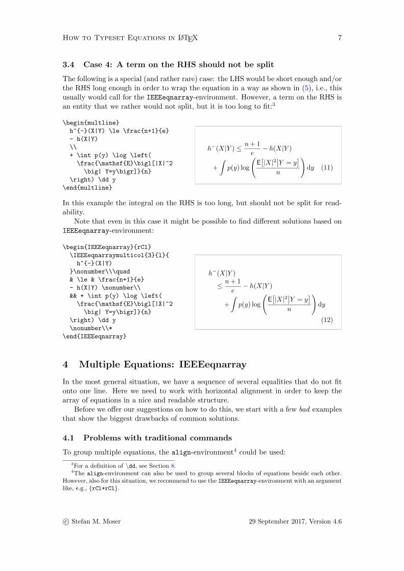
3.4 Case 4: A term on the RHS should not be split
The following is a special (and rather rare) case: the LHS would be short enough and/orthe RHS long enough in order to wrap the equation in a way as shown in (5), i.e., thisusually would call for the IEEEeqnarray-environment. However, a term on the RHS isan entity that we rather would not split, but it is too long to fit:3
\begin{multline}
h^{-}(X|Y) \le \frac{n+1}{e}
- h(X|Y)
\\
+ \int p(y) \log \left(
\frac{\mathsf{E}\bigl[|X|^2
\big| Y=y\bigr]}{n}
\right) \dd y
\end{multline}
h−(X|Y ) ≤ n+ 1
e− h(X|Y )
+
∫p(y) log
(E[|X|2
∣∣Y = y]
n
)dy (11)
In this example the integral on the RHS is too long, but should not be split for read-ability.
Note that even in this case it might be possible to find different solutions based onIEEEeqnarray-environment:
\begin{IEEEeqnarray}{rCl}
\IEEEeqnarraymulticol{3}{l}{
h^{-}(X|Y)
}\nonumber\\\quad
& \le & \frac{n+1}{e}
- h(X|Y) \nonumber\\
&& + \int p(y) \log \left(
\frac{\mathsf{E}\bigl[|X|^2
\big| Y=y\bigr]}{n}
\right) \dd y
\nonumber\\*
\end{IEEEeqnarray}
h−(X|Y )
≤ n+ 1
e− h(X|Y )
+
∫p(y) log
(E[|X|2
∣∣Y = y]
n
)dy
(12)
4 Multiple Equations: IEEEeqnarray
In the most general situation, we have a sequence of several equalities that do not fitonto one line. Here we need to work with horizontal alignment in order to keep thearray of equations in a nice and readable structure.
Before we offer our suggestions on how to do this, we start with a few bad examplesthat show the biggest drawbacks of common solutions.
4.1 Problems with traditional commands
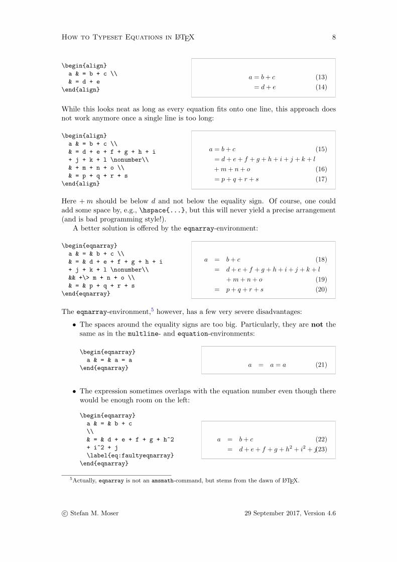
To group multiple equations, the align-environment4 could be used:
3For a definition of \dd, see Section 8.4The align-environment can also be used to group several blocks of equations beside each other.
However, also for this situation, we recommend to use the IEEEeqnarray-environment with an argumentlike, e.g., {rCl+rCl}.
c© Stefan M. Moser 29 September 2017, Version 4.6
How to Typeset Equations in LATEX 8
\begin{align}
a & = b + c \\
& = d + e
\end{align}
a = b+ c (13)
= d+ e (14)
While this looks neat as long as every equation fits onto one line, this approach doesnot work anymore once a single line is too long:
\begin{align}
a & = b + c \\
& = d + e + f + g + h + i
+ j + k + l \nonumber\\
& + m + n + o \\
& = p + q + r + s
\end{align}
a = b+ c (15)
= d+ e+ f + g + h+ i+ j + k + l
+m+ n+ o (16)
= p+ q + r + s (17)
Here +m should be below d and not below the equality sign. Of course, one couldadd some space by, e.g., \hspace{...}, but this will never yield a precise arrangement(and is bad programming style!).
A better solution is offered by the eqnarray-environment:
\begin{eqnarray}
a & = & b + c \\
& = & d + e + f + g + h + i
+ j + k + l \nonumber\\
&& +\> m + n + o \\
& = & p + q + r + s
\end{eqnarray}
a = b+ c (18)
= d+ e+ f + g + h+ i+ j + k + l
+m+ n+ o (19)
= p+ q + r + s (20)
The eqnarray-environment,5 however, has a few very severe disadvantages:
• The spaces around the equality signs are too big. Particularly, they are not thesame as in the multline- and equation-environments:
\begin{eqnarray}
a & = & a = a
\end{eqnarray} a = a = a (21)
• The expression sometimes overlaps with the equation number even though therewould be enough room on the left:
\begin{eqnarray}
a & = & b + c
\\
& = & d + e + f + g + h^2
+ i^2 + j
\label{eq:faultyeqnarray}
\end{eqnarray}
a = b+ c (22)
= d+ e+ f + g + h2 + i2 + j(23)
5Actually, eqnarray is not an amsmath-command, but stems from the dawn of LATEX.
c© Stefan M. Moser 29 September 2017, Version 4.6

How to Typeset Equations in LATEX 9
• The eqnarray-environment offers a command \lefteqn{...} that can be usedwhen the LHS is too long:
\begin{eqnarray}
\lefteqn{a + b + c + d
+ e + f + g + h}\nonumber\\
& = & i + j + k + l + m
\\
& = & n + o + p + q + r + s
\end{eqnarray}
a+ b+ c+ d+ e+ f + g + h
= i+ j + k + l +m (24)
= n+ o+ p+ q + r + s (25)
Unfortunately, this command is faulty: if the RHS is too short, the array is notproperly centered:
\begin{eqnarray}
\lefteqn{a + b + c + d
+ e + f + g + h}
\nonumber\\
& = & i + j
\end{eqnarray}
a+ b+ c+ d+ e+ f + g + h
= i+ j (26)
Moreover, it is very complicated to change the horizontal alignment of the equalitysign on the second line.
Thus:
NEVER ever use the eqnarray-environment!
To overcome these problems we recommend the IEEEeqnarray-environment.
4.2 Solution: basic usage of IEEEeqnarray
The IEEEeqnarray-environment is a very powerful command with many options. Inthis manual we will only introduce some of the most important functionalities. Formore information we refer to the official manual.6 First of all, in order to be able touse the IEEEeqnarray-environment, one needs to include the package7 IEEEtrantools.Include the following line in the header of your document:
\usepackage{IEEEtrantools}
The strength of IEEEeqnarray is the possibility of specifying the number of columnsin the equation array. Usually, this specification will be {rCl}, i.e., three columns, thefirst column right-justified, the middle one centered with a little more space around
6The official manual IEEEtran HOWTO.pdf is distributed together with this short introduction. Thepart about IEEEeqnarray can be found in Appendix F.
7This package is also distributed together with this manual, but it is already included in any up-to-date LATEX distribution. Note that if a document uses the IEEEtran-class, then IEEEtrantools isloaded automatically and must not be included separately.
c© Stefan M. Moser 29 September 2017, Version 4.6

How to Typeset Equations in LATEX 10
it (therefore we specify capital C instead of lower-case c) and the third column left-justified:
\begin{IEEEeqnarray}{rCl}
a & = & b + c
\\
& = & d + e + f + g + h
+ i + j + k \nonumber\\
&& +\> l + m + n + o
\\
& = & p + q + r + s
\end{IEEEeqnarray}
a = b+ c (27)
= d+ e+ f + g + h+ i+ j + k
+ l +m+ n+ o (28)
= p+ q + r + s (29)
However, we can specify any number of needed columns. For example, {c} will give onlyone column (which is centered) or {rCl"l} will add a fourth, left-justified column thatis shifted to the right (the spacing is defined by the "), e.g., for additional specifications.Moreover, beside l, c, r, L, C, R for math mode entries, there also exists s, t, u forleft, centered, and right text mode entries, respectively. And additional spacing can beadded by . and / and ? and " in increasing order.8 More details about the usage ofIEEEeqnarray will be given in Section 5.
Note that in contrast to eqnarray the spaces around the equality signs are correct.
4.3 A remark about consistency
There are three more issues that have not been mentioned so far, but that might causeinconsistencies when all three environments, equation, multline, and IEEEeqnarray,are used intermixedly:
• multline allows for an equation starting on top of a page, while equation andIEEEeqnarray try to put a line of text first, before the equation starts. Moreover,the spacing before and after the environment is not exactly identical for equation,multline, and IEEEeqnarray.
• equation uses an automatic mechanism to move the equation number onto thenext line if the expression is too long. While this is convenient, sometimes theequation number is forced onto the next line, even if there was still enough spaceavailable on the line:
\begin{equation}
a = \sum_{k=1}^n\sum_{\ell=1}^n
\sin \bigl(2\pi \, b_k \,
c_{\ell} \, d_k \, e_{\ell} \,
f_k \, g_{\ell} \, h \bigr)
\end{equation}
a =
n∑k=1
n∑`=1
sin(2π bk c` dk e` fk g` h
)(30)
With IEEEeqnarray the placement of the equation number is fully under ourcontrol:
8For examples of spacing, we refer to Section 6.2. More spacing types can be found in the examplesgiven in Sections 5.3 and 6.9, and in the official manual.
c© Stefan M. Moser 29 September 2017, Version 4.6

How to Typeset Equations in LATEX 11
\begin{IEEEeqnarray}{c}
a = \sum_{k=1}^n\sum_{\ell=1}^n
\sin \bigl(2\pi \, b_k \,
c_{\ell} \, d_k \, e_{\ell} \,
f_k \, g_{\ell} \, h \bigr)
\IEEEeqnarraynumspace
\label{eq:labelc1}
\end{IEEEeqnarray}
a =
n∑k=1
n∑`=1
sin(2π bk c` dk e` fk g` h
)(31)
or
\begin{IEEEeqnarray}{c}
a = \sum_{k=1}^n\sum_{\ell=1}^n
\sin \bigl(2\pi \, b_k \,
c_{\ell} \, d_k \, e_{\ell} \,
f_k \, g_{\ell} \, h \bigr)
\nonumber\\*
\label{eq:labelc2}
\end{IEEEeqnarray}
a =
n∑k=1
n∑`=1
sin(2π bk c` dk e` fk g` h
)(32)
• equation forces the equation number to appear in normal font, even if the equa-tion is within an environment9 of different font:
\textbf{\textit{\color{red}
This is our main result:
\begin{equation}
a = b + c
\end{equation}}}
This is our main result:
a = b+ c (33)
IEEEeqnarray respects the settings of the environment:
\textbf{\textit{\color{red}
This is our main result:
\begin{IEEEeqnarray}{c}
a = b + c
\end{IEEEeqnarray}}}
This is our main result:
a = b+ c (34)
If this is undesired, one can change the behavior of IEEEeqnarray to behave10
like equation:
\renewcommand{\theequationdis}{{\normalfont (\theequation)}}
\renewcommand{\theIEEEsubequationdis}{{\normalfont (\theIEEEsubequation)}}
9A typical example of such a situation is an equation inside of a theorem that is typeset in italicfont.
10For an explanation of the subnumbering, see Section 5.4.
c© Stefan M. Moser 29 September 2017, Version 4.6

How to Typeset Equations in LATEX 12
\textbf{\textit{\color{red}
This is our main result:
\begin{IEEEeqnarray}{rCl}
a & = & b + c \\
& = & d + e \IEEEyesnumber
\IEEEyessubnumber
\end{IEEEeqnarray}}}
This is our main result:
a = b+ c (35)
= d+ e (36a)
4.4 Using IEEEeqnarray for all situations
As seen above, there might be reason to rely on IEEEeqnarray exclusively in all situ-ations.
To replace an equation-environment we use IEEEeqnarray with only one column{c}, see (31) and (32) above.
Emulating multline is slightly more complicated: we implement IEEEeqnarray
with only one column {l}, use \IEEEeqnarraymulticol11 after the line-break(s) toadapt the column type of the new line, and manually add some shift:
\begin{IEEEeqnarray*}{l}
a + b + c + d + e + f
\\ \qquad
+\> g + h + i + j + k + l
\qquad \\
\IEEEeqnarraymulticol{1}{r}{
+\> m + n + o + p + q }
\IEEEyesnumber
\end{IEEEeqnarray*}
a+ b+ c+ d+ e+ f
+ g + h+ i+ j + k + l
+m+ n+ o+ p+ q (37)
5 More Details about IEEEeqnarray
In the following we will describe how we use IEEEeqnarray to solve the most commonsituations.
5.1 Shift to the left: IEEEeqnarraynumspace
If a line overlaps with the equation number as in (23), the command
\IEEEeqnarraynumspace
can be used. It has to be added in the corresponding line and makes sure that thewhole equation array is shifted by the size of the equation numbers (the shift dependson the size of the number!). Instead of
11For a more detailed explanation of this command, see Section 5.2.
c© Stefan M. Moser 29 September 2017, Version 4.6

How to Typeset Equations in LATEX 13
\begin{IEEEeqnarray}{rCl}
a & = & b + c
\\
& = & d + e + f + g + h
+ i + j + k + m
\\
& = & l + n + o
\end{IEEEeqnarray}
a = b+ c (38)
= d+ e+ f + g + h+ i+ j + k +m(39)
= l + n+ o (40)
we get
\begin{IEEEeqnarray}{rCl}
a & = & b + c
\\
& = & d + e + f + g + h
+ i + j + k + m
\IEEEeqnarraynumspace\\
& = & l + n + o
\end{IEEEeqnarray}
a = b+ c (41)
= d+ e+ f + g + h+ i+ j + k +m (42)
= l + n+ o (43)
Note that if there is not enough space on the line, this shift will force the numbersto cross the right boundary of the text. So be sure to check the result!
The boundary of the text can be
seen from this text above the
equation array. The number is
clearly beyond it:
\begin{IEEEeqnarray}{rCl}
a & = & d + e + f + g + h
+ i + j + k + l + m + n
\IEEEeqnarraynumspace
\end{IEEEeqnarray}
The boundary of the text can be seen fromthis text above the equation array. The num-ber is clearly beyond it:
a = d+ e+ f + g + h+ i+ j + k + l +m+ n(44)
In such a case one needs to wrap the equation somewhere.
5.2 First line too long: IEEEeqnarraymulticol
If the LHS is too long and as a replacement for the faulty \lefteqn{}-command,IEEEeqnarray offers the \IEEEeqnarraymulticol-command, which works in all situ-ations:
\begin{IEEEeqnarray}{rCl}
\IEEEeqnarraymulticol{3}{l}{
a + b + c + d + e + f
+ g + h
}\nonumber\\* \quad
& = & i + j
\\
& = & k + l + m
\end{IEEEeqnarray}
a+ b+ c+ d+ e+ f + g + h
= i+ j (45)
= k + l +m (46)
The usage is identical to the \multicolumns-command in the tabular-environment.The first argument {3} specifies that three columns shall be combined into one, which
c© Stefan M. Moser 29 September 2017, Version 4.6
How to Typeset Equations in LATEX 14
will be left-justified {l}. We usually add a * to the line-break \\ to prevent a page-break at this position.
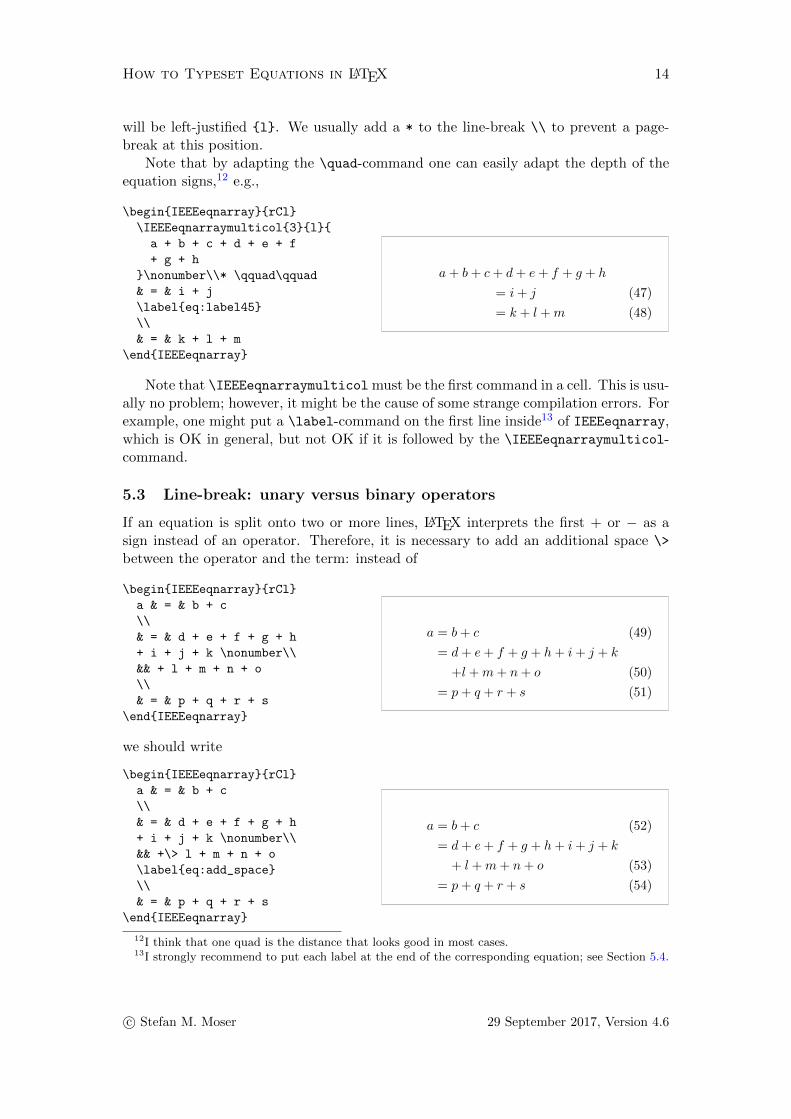
Note that by adapting the \quad-command one can easily adapt the depth of theequation signs,12 e.g.,
\begin{IEEEeqnarray}{rCl}
\IEEEeqnarraymulticol{3}{l}{
a + b + c + d + e + f
+ g + h
}\nonumber\\* \qquad\qquad
& = & i + j
\label{eq:label45}
\\
& = & k + l + m
\end{IEEEeqnarray}
a+ b+ c+ d+ e+ f + g + h
= i+ j (47)
= k + l +m (48)
Note that \IEEEeqnarraymulticol must be the first command in a cell. This is usu-ally no problem; however, it might be the cause of some strange compilation errors. Forexample, one might put a \label-command on the first line inside13 of IEEEeqnarray,which is OK in general, but not OK if it is followed by the \IEEEeqnarraymulticol-command.
5.3 Line-break: unary versus binary operators
If an equation is split onto two or more lines, LATEX interprets the first + or − as asign instead of an operator. Therefore, it is necessary to add an additional space \>
between the operator and the term: instead of
\begin{IEEEeqnarray}{rCl}
a & = & b + c
\\
& = & d + e + f + g + h
+ i + j + k \nonumber\\
&& + l + m + n + o
\\
& = & p + q + r + s
\end{IEEEeqnarray}
a = b+ c (49)
= d+ e+ f + g + h+ i+ j + k
+l +m+ n+ o (50)
= p+ q + r + s (51)
we should write
\begin{IEEEeqnarray}{rCl}
a & = & b + c
\\
& = & d + e + f + g + h
+ i + j + k \nonumber\\
&& +\> l + m + n + o
\label{eq:add_space}
\\
& = & p + q + r + s
\end{IEEEeqnarray}
a = b+ c (52)
= d+ e+ f + g + h+ i+ j + k
+ l +m+ n+ o (53)
= p+ q + r + s (54)
12I think that one quad is the distance that looks good in most cases.13I strongly recommend to put each label at the end of the corresponding equation; see Section 5.4.
c© Stefan M. Moser 29 September 2017, Version 4.6

How to Typeset Equations in LATEX 15
(Compare the space between + and l!)Attention: The distinction between the unary operator (sign) and the binary
operator (addition/subtraction) is not satisfactorily solved in LATEX.14 In some casesLATEX will automatically assume that the operator cannot be unary and will thereforeadd additional spacing. This happens, e.g., in front of
• an operator name like \log, \sin, \det, \max, etc.,
• an integral \int or sum \sum,
• a bracket with adaptive size using \left and \right (this is in contrast to normalbrackets or brackets with fixed size like \bigl( and \bigr)).
This decision, however, might be faulty. E.g., it makes perfect sense to have a unaryoperator in front of the logarithm:
\begin{IEEEeqnarray*}{rCl"s}
\log \frac{1}{a}
& = & -\log a
& (binary, wrong) \\
& = & -{\log a}
& (unary, correct)
\end{IEEEeqnarray*}
log1
a= − log a (binary, wrong)
= −log a (unary, correct)
In this case, you have to correct it manually. Unfortunately, there is no clean way ofdoing this. To enforce a unary operator, enclosing the expression following the unaryoperator and/or the unary operator itself into curly brackets {...} will usually work.For the opposite direction, i.e., to enforce a binary operator (as, e.g., needed in (53)),the only option is to put in the correct space \> manually.15
In the following example, compare the spacing between the first minus-sign on theRHS and b (or log b):
\begin{IEEEeqnarray*}{rCl’s}
a & = & - b - b - c
& (default unary) \\
& = & {-} {b} - b - c
& (default unary, no effect) \\
& = & -\> b - b - c
& (changed to binary) \\
& = & - \log b - b - d
& (default binary) \\
& = & {-} {\log b} - b - d
& (changed to unary) \\
& = & - \log b - b {-} d
& (changed $-d$ to unary)
\end{IEEEeqnarray*}
a = −b− b− c (default unary)
= −b− b− c (default unary, no effect)
= − b− b− c (changed to binary)
= − log b− b− d (default binary)
= −log b− b− d (changed to unary)
= − log b− b−d (changed −d to unary)
14The problem actually goes back to TEX.15This spacing command adds the flexible space medmuskip = 4mu plus 2mu minus 4mu.
c© Stefan M. Moser 29 September 2017, Version 4.6

How to Typeset Equations in LATEX 16
We learn:
Whenever you wrap a line, quickly check the result and verify that the spacingis correct!
5.4 Equation numbers and subnumbers
While IEEEeqnarray assigns an equation number to all lines, the starred versionIEEEeqnarray* suppresses all numbers. This behavior can be changed individuallyper line by the commands
\IEEEyesnumber and \IEEEnonumber (or \nonumber).
For subnumbering the corresponding commands
\IEEEyessubnumber and \IEEEnosubnumber
are available. These four commands only affect the line on which they are invoked,however, there also exist starred versions
\IEEEyesnumber*, \IEEEnonumber*,\IEEEyessubnumber*, \IEEEnosubnumber*
that will remain active until the end of the IEEEeqnarray-environment or until anotherstarred command is invoked.
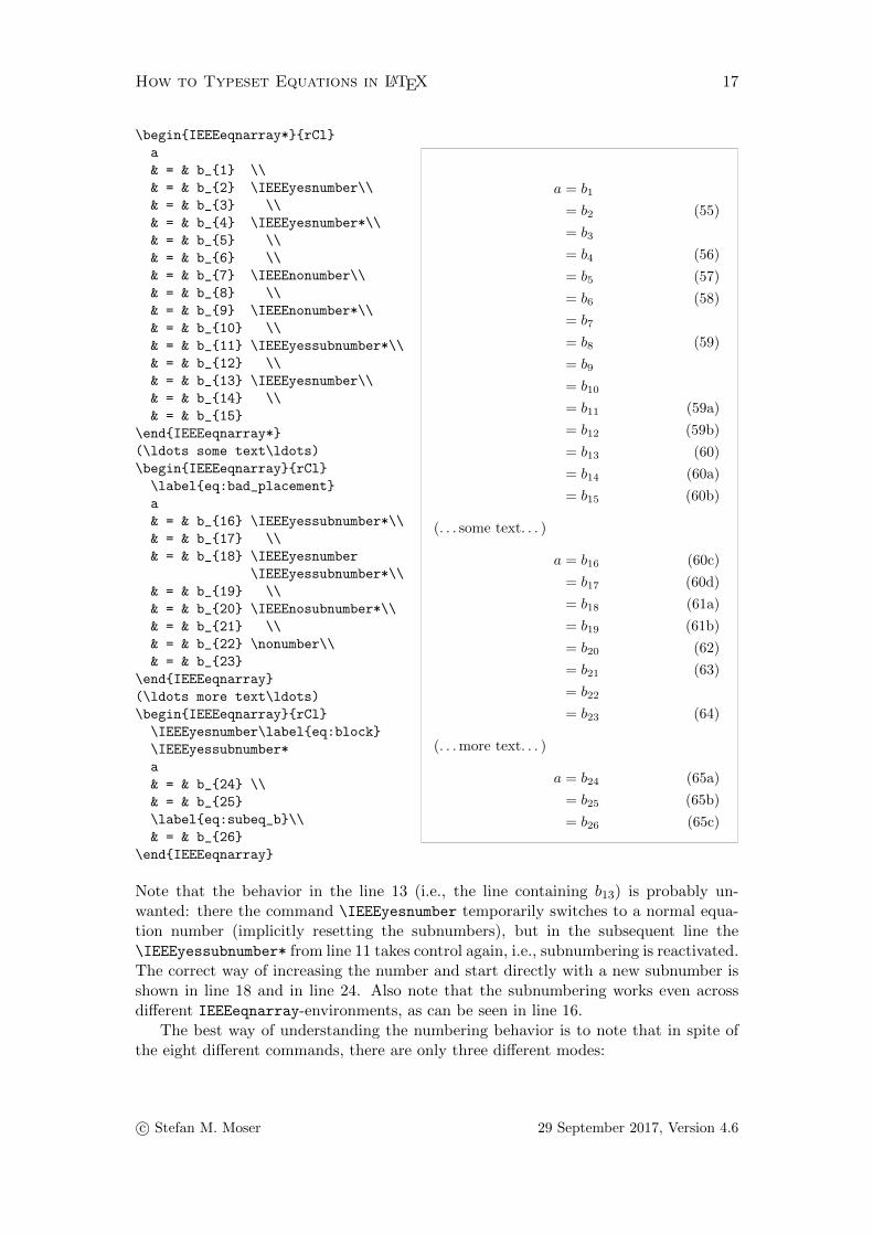
Consider the following extensive example.
c© Stefan M. Moser 29 September 2017, Version 4.6
How to Typeset Equations in LATEX 17
\begin{IEEEeqnarray*}{rCl}
a
& = & b_{1} \\
& = & b_{2} \IEEEyesnumber\\
& = & b_{3} \\
& = & b_{4} \IEEEyesnumber*\\
& = & b_{5} \\
& = & b_{6} \\
& = & b_{7} \IEEEnonumber\\
& = & b_{8} \\
& = & b_{9} \IEEEnonumber*\\
& = & b_{10} \\
& = & b_{11} \IEEEyessubnumber*\\
& = & b_{12} \\
& = & b_{13} \IEEEyesnumber\\
& = & b_{14} \\
& = & b_{15}
\end{IEEEeqnarray*}
(\ldots some text\ldots)
\begin{IEEEeqnarray}{rCl}
\label{eq:bad_placement}
a
& = & b_{16} \IEEEyessubnumber*\\
& = & b_{17} \\
& = & b_{18} \IEEEyesnumber
\IEEEyessubnumber*\\
& = & b_{19} \\
& = & b_{20} \IEEEnosubnumber*\\
& = & b_{21} \\
& = & b_{22} \nonumber\\
& = & b_{23}
\end{IEEEeqnarray}
(\ldots more text\ldots)
\begin{IEEEeqnarray}{rCl}
\IEEEyesnumber\label{eq:block}
\IEEEyessubnumber*
a
& = & b_{24} \\
& = & b_{25}
\label{eq:subeq_b}\\
& = & b_{26}
\end{IEEEeqnarray}
a = b1
= b2 (55)
= b3
= b4 (56)
= b5 (57)
= b6 (58)
= b7
= b8 (59)
= b9
= b10
= b11 (59a)
= b12 (59b)
= b13 (60)
= b14 (60a)
= b15 (60b)
(. . . some text. . . )
a = b16 (60c)
= b17 (60d)
= b18 (61a)
= b19 (61b)
= b20 (62)
= b21 (63)
= b22
= b23 (64)
(. . . more text. . . )
a = b24 (65a)
= b25 (65b)
= b26 (65c)
Note that the behavior in the line 13 (i.e., the line containing b13) is probably un-wanted: there the command \IEEEyesnumber temporarily switches to a normal equa-tion number (implicitly resetting the subnumbers), but in the subsequent line the\IEEEyessubnumber* from line 11 takes control again, i.e., subnumbering is reactivated.The correct way of increasing the number and start directly with a new subnumber isshown in line 18 and in line 24. Also note that the subnumbering works even acrossdifferent IEEEeqnarray-environments, as can be seen in line 16.
The best way of understanding the numbering behavior is to note that in spite ofthe eight different commands, there are only three different modes:
c© Stefan M. Moser 29 September 2017, Version 4.6

How to Typeset Equations in LATEX 18
1. No equation number (corresponding to \IEEEnonumber).
2. A normal equation number (corresponding to \IEEEyesnumber): the equationcounter is incremented and then displayed.
3. An equation number with subnumber (corresponding to \IEEEyessubnumber):only the subequation counter is incremented and then both the equation and thesubequation numbers are displayed. (Attention: If the equation number shall beincremented as well, which is usually the case for the start of a new subnumbering,then also \IEEEyesnumber has to be given!)
The understanding of the working of these three modes is also important when usinglabels to refer to equations. Note that the label referring to an equation with a sub-number must always be given after the \IEEEyessubnumber command. Otherwise thelabel will refer to the current (or future) main number, which is usually undesired. E.g.,the label eq:bad_placement in line 16 points16 (wrongly) to (61).
A correct example is shown in (65) and (65b): the label \label{eq:block} refersto the whole block, and the label \label{eq:subeq_b} refers to the correspondingsubequation.
We learn:
A label should always be put at the end of the equation it belongs to(i.e., right in front of the line-break \\).
Besides preventing unwanted results, this rules also increases the readability of thesource code and prevents a compilation error in the situation of an \IEEEeqnarraymul
ticol-command after a label-definition.
Hyperlinks
As this document demonstrates, hyperlinking works (almost) seamlessly with IEEEeqn
array. For this document we simply included
\usepackage[colorlinks=true,linkcolor=blue]{hyperref}
in the header, and then all references automatically become hyperlinks.There is only one small issue that you might have noticed already: the reference
(65) points into nirvana. The reason for this is that there is no actual equation number(65) generated and therefore hyperref does not create the corresponding hyperlink.This can be fixed, but requires some more advanced LATEX-programming. Copy-pastethe following code into the document header (or your stylefile):
16To understand this, note that when the label-command was invoked, subnumbering was deactiv-ated. So the label only refers to a normal equation number. However, no such number was active thereeither, so the label is passed on to line 18 where the equation counter is incremented for the first time.
c© Stefan M. Moser 29 September 2017, Version 4.6

How to Typeset Equations in LATEX 19
\makeatletter
\def\IEEElabelanchoreqn#1{\bgroup
\def\@currentlabel{\p@equation\theequation}\relax
\def\@currentHref{\@IEEEtheHrefequation}\label{#1}\relax
\Hy@raisedlink{\hyper@anchorstart{\@currentHref}}\relax
\Hy@raisedlink{\hyper@anchorend}\egroup}
\makeatother
\newcommand{\subnumberinglabel}[1]{\IEEEyesnumber
\IEEEyessubnumber*\IEEElabelanchoreqn{#1}}
Now, \IEEElabelanchoreqn{...} creates an anchor for a hyperlink to an invisibleequation number. The command \subnumberinglabel then sets this anchor and atthe same time activates subnumbering, simplifying our typesetting:
We have
\begin{IEEEeqnarray}{rCl}
\subnumberinglabel{eq:block2}
a & = & b + c
\label{eq:block2_eq1}\\
& = & d + e
\label{eq:block2_eq2}
\end{IEEEeqnarray}
and
\begin{IEEEeqnarray}{c}
\IEEEyessubnumber*
f = g - h + i
\label{eq:block2_eq3}
\end{IEEEeqnarray}
We have
a = b+ c (66a)
= d+ e (66b)
and
f = g − h+ i (66c)
Now (66) refers to the whole block (the hyperlink points to the first line of the firstequation array), and (66a), (66b), and (66c) point to the corresponding subequations.
Alternative subnumbers: subequations
We conclude this section by remarking that IEEEeqnarray is fully compatible with thesubequations-environment. Thus, (66) can also be created in the following way:
We have
\begin{subequations}
\label{eq:block2_alt}
\begin{IEEEeqnarray}{rCl}
a & = & b + c
\label{eq:block2_eq1_alt}\\
& = & d + e
\label{eq:block2_eq2_alt}
\end{IEEEeqnarray}
and
\begin{IEEEeqnarray}{c}
f = g - h + i
\label{eq:block2_eq3_alt}
\end{IEEEeqnarray}
\end{subequations}
We have
a = b+ c (67a)
= d+ e (67b)
and
f = g − h+ i (67c)
c© Stefan M. Moser 29 September 2017, Version 4.6

How to Typeset Equations in LATEX 20
Note, however, that the hyperlink of (67) points to the beginning of the subequations-environment and not onto the first line of the equation array as in (66)!
5.5 Page-breaks inside of IEEEeqnarray
By default, amsmath does not allow page-breaks within multiple equations, which usu-ally is too restrictive, particularly, if a document contains long equation arrays. Thisbehavior can be changed by putting the following line into the document header:
\interdisplaylinepenalty=xx
Here, xx is some number: the larger this number, the less likely it is that an equationarray is broken over to the next page. So, a value 0 fully allows page-breaks, a value2500 allows page-breaks, but only if LATEX finds no better solution, or a value 10’000basically prevents page-breaks (which is the default given in amsmath).17
6 Advanced Typesetting
In this section we address a couple of more advanced typesetting problems and tools.
6.1 Aligning several separate equation arrays
Sometimes it looks elegant if one can align not just the equations within one array, butbetween several arrays (with regular text in between). This can be achieved by actuallycreating one single large array and add additional text in between. For example, (66)could be typeset as follows:
We have
\begin{IEEEeqnarray}{rCl}
\subnumberinglabel{eq:block3}
a & = & b + c
\label{eq:block3_eq1}\\
& = & d + e
\label{eq:block3_eq2}\\
\noalign{\noindent and
\vspace{2\jot}}
f & = & g - h + i
\label{eq:block3_eq3}
\end{IEEEeqnarray}
We have
a = b+ c (68a)
= d+ e (68b)
and
f = g − h+ i (68c)
Note how the equality-sign in (68c) is aligned to the equality-signs of (68a) and (68b).In the code, we add the text “and” into the array using the command \noalign{...}
and then manually add some vertical spacing.
17I usually use a value 1000 that in principle allows page-breaks, but still asks LATEX to check if thereis no other way.
c© Stefan M. Moser 29 September 2017, Version 4.6
How to Typeset Equations in LATEX 21
6.2 IEEEeqnarraybox: general tables and arrays
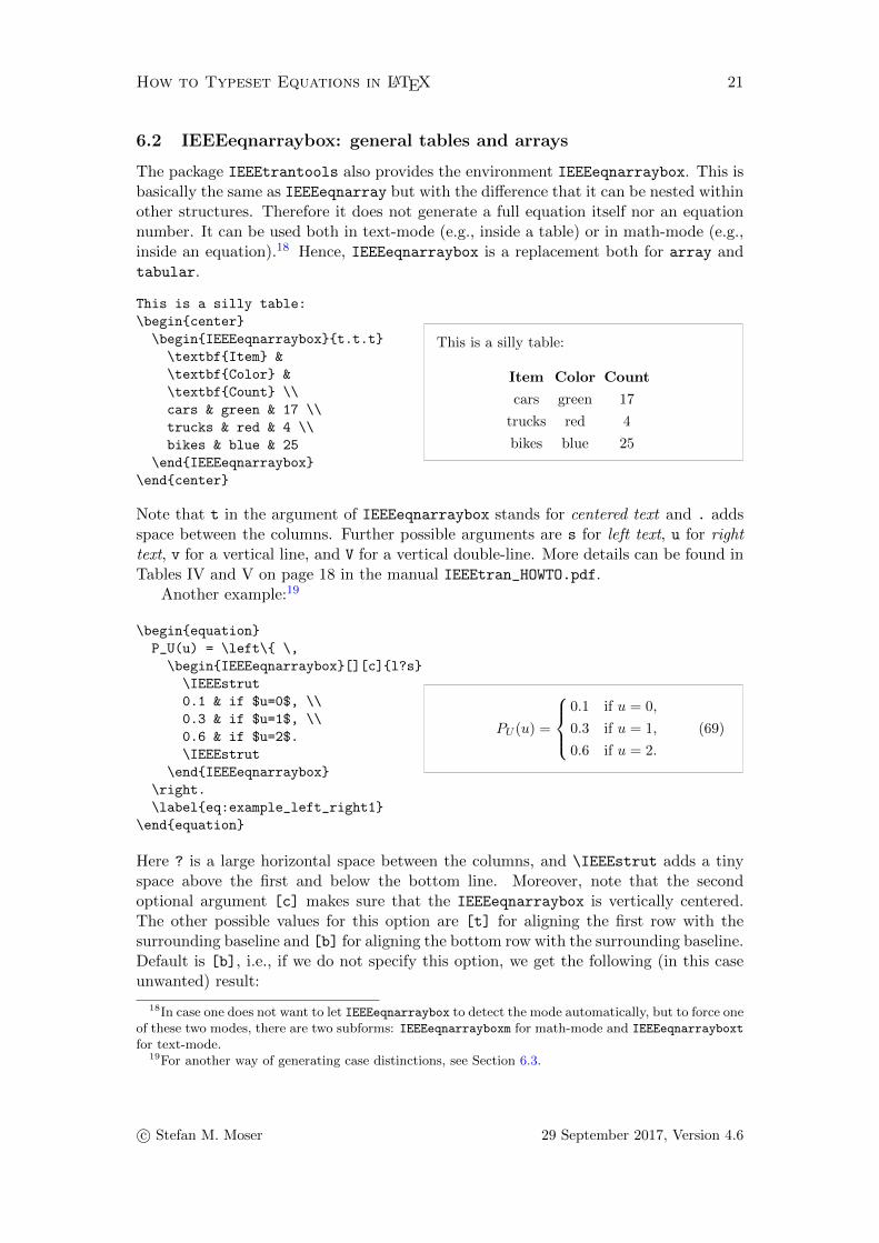
The package IEEEtrantools also provides the environment IEEEeqnarraybox. This isbasically the same as IEEEeqnarray but with the difference that it can be nested withinother structures. Therefore it does not generate a full equation itself nor an equationnumber. It can be used both in text-mode (e.g., inside a table) or in math-mode (e.g.,inside an equation).18 Hence, IEEEeqnarraybox is a replacement both for array andtabular.
This is a silly table:
\begin{center}
\begin{IEEEeqnarraybox}{t.t.t}
\textbf{Item} &
\textbf{Color} &
\textbf{Count} \\
cars & green & 17 \\
trucks & red & 4 \\
bikes & blue & 25
\end{IEEEeqnarraybox}
\end{center}
This is a silly table:
Item Color Count
cars green 17
trucks red 4
bikes blue 25
Note that t in the argument of IEEEeqnarraybox stands for centered text and . addsspace between the columns. Further possible arguments are s for left text, u for righttext, v for a vertical line, and V for a vertical double-line. More details can be found inTables IV and V on page 18 in the manual IEEEtran_HOWTO.pdf.
Another example:19
\begin{equation}
P_U(u) = \left\{ \,
\begin{IEEEeqnarraybox}[][c]{l?s}
\IEEEstrut
0.1 & if $u=0$, \\
0.3 & if $u=1$, \\
0.6 & if $u=2$.
\IEEEstrut
\end{IEEEeqnarraybox}
\right.
\label{eq:example_left_right1}
\end{equation}
PU (u) =
0.1 if u = 0,
0.3 if u = 1,
0.6 if u = 2.
(69)
Here ? is a large horizontal space between the columns, and \IEEEstrut adds a tinyspace above the first and below the bottom line. Moreover, note that the secondoptional argument [c] makes sure that the IEEEeqnarraybox is vertically centered.The other possible values for this option are [t] for aligning the first row with thesurrounding baseline and [b] for aligning the bottom row with the surrounding baseline.Default is [b], i.e., if we do not specify this option, we get the following (in this caseunwanted) result:
18In case one does not want to let IEEEeqnarraybox to detect the mode automatically, but to force oneof these two modes, there are two subforms: IEEEeqnarrayboxm for math-mode and IEEEeqnarrayboxt
for text-mode.19For another way of generating case distinctions, see Section 6.3.
c© Stefan M. Moser 29 September 2017, Version 4.6

How to Typeset Equations in LATEX 22
\begin{equation*}
P_U(u) = \left\{ \,
\begin{IEEEeqnarraybox}{l?s}
0.1 & if $u=0$, \\
0.3 & if $u=1$, \\
0.6 & if $u=2$.
\end{IEEEeqnarraybox}
\right.
\end{equation*}
PU (u) =
0.1 if u = 0,
0.3 if u = 1,
0.6 if u = 2.
We also dropped \IEEEstrut here with the result that the curly bracket is slightly toosmall at the top line.
Actually, these manually placed \IEEEstrut commands are rather tiring. More-over, when we would like to add vertical lines in a table, a first naive application ofIEEEeqnarraybox yields the following:
\begin{equation*}
\begin{IEEEeqnarraybox}{c’c;v;c’c’c}
D_1 & D_2 && X_1 & X_2
& X_3
\\\hline
0 & 0 && +1 & +1 & +1\\
0 & 1 && +1 & -1 & -1\\
1 & 0 && -1 & +1 & -1\\
1 & 1 && -1 & -1 & +1
\end{IEEEeqnarraybox}
\end{equation*}
D1 D2 X1 X2 X3
0 0 +1 +1 +1
0 1 +1 −1 −1
1 0 −1 +1 −1
1 1 −1 −1 +1
We see that IEEEeqnarraybox makes a complete line-break after each line. This is ofcourse unwanted. Therefore, the command \IEEEeqnarraystrutmode is provided thatswitches the spacing system completely over to struts:
\begin{equation*}
\begin{IEEEeqnarraybox}[
\IEEEeqnarraystrutmode
]{c’c;v;c’c’c}
D_1 & D_2 && X_1 & X_2 & X_3
\\\hline
0 & 0 && +1 & +1 & +1\\
0 & 1 && +1 & -1 & -1\\
1 & 0 && -1 & +1 & -1\\
1 & 1 && -1 & -1 & +1
\end{IEEEeqnarraybox}
\end{equation*}
D1 D2 X1 X2 X3
0 0 +1 +1 +10 1 +1 −1 −11 0 −1 +1 −11 1 −1 −1 +1
The strutmode also easily allows to ask for more “air” between each line and therebyeliminating the need of manually adding an \IEEEstrut:
c© Stefan M. Moser 29 September 2017, Version 4.6

How to Typeset Equations in LATEX 23
\begin{equation*}
\begin{IEEEeqnarraybox}[
\IEEEeqnarraystrutmode
\IEEEeqnarraystrutsizeadd{3pt}
{1pt}
]{c’c/v/c’c’c}
D_1 & D_2 & & X_1 & X_2 & X_3
\\\hline
0 & 0 && +1 & +1 & +1\\
0 & 1 && +1 & -1 & -1\\
1 & 0 && -1 & +1 & -1\\
1 & 1 && -1 & -1 & +1
\end{IEEEeqnarraybox}
\end{equation*}
D1 D2 X1 X2 X3
0 0 +1 +1 +1
0 1 +1 −1 −1
1 0 −1 +1 −1
1 1 −1 −1 +1
Here the first argument of \IEEEeqnarraystrutsizeadd{3pt}{1pt} adds space aboveinto each line, the second adds space below into each line.
6.3 Case distinctions
Case distinctions can be generated using IEEEeqnarraybox as shown in Section 6.2.However, in the standard situation the usage of cases is simpler and we thereforerecommend to use this:
\begin{equation}
P_U(u) =
\begin{cases}
0.1 & \text{if } u=0,
\\
0.3 & \text{if } u=1,
\\
0.6 & \text{if } u=2.
\end{cases}
\end{equation}
PU (u) =
0.1 if u = 0,
0.3 if u = 1,
0.6 if u = 2.
(70)
For more complicated examples we do need to rely on IEEEeqnarraybox:
c© Stefan M. Moser 29 September 2017, Version 4.6

How to Typeset Equations in LATEX 24
\begin{equation}
\left.
\begin{IEEEeqnarraybox}[\IEEEeqnarraystrutmode
\IEEEeqnarraystrutsizeadd{2pt}{2pt}][c]{rCl}
x & = & a + b\\
y & = & a - b
\end{IEEEeqnarraybox}
\, \right\} \iff \left\{ \,
\begin{IEEEeqnarraybox}[
\IEEEeqnarraystrutmode
\IEEEeqnarraystrutsizeadd{7pt}
{7pt}][c]{rCl}
a & = & \frac{x}{2} + \frac{y}{2}
\\
b & = & \frac{x}{2} - \frac{y}{2}
\end{IEEEeqnarraybox}
\right.
\label{eq:example_left_right2}
\end{equation}
x = a+ b
y = a− b
}⇐⇒
a =
x
2+y
2
b =x
2− y
2
(71)
If we would like to have a distinct equation number for each case, the package
\usepackage{cases}
provides by far the easiest solution:
\begin{numcases}{|x|=}
x & for $x \geq 0$,
\\
-x & for $x < 0$.
\end{numcases}
|x| ={x for x ≥ 0, (72)
−x for x < 0. (73)
Note the differences to the usual cases-environment:
• The left-hand side must be typeset as compulsory argument to the environment.
• The second column is not in math-mode but directly in text-mode.
For subnumbering we can use the corresponding subnumcases-environment:
\begin{subnumcases}{P_U(u)=}
0.1 & if $u=0$,
\\
0.3 & if $u=1$,
\\
0.6 & if $u=2$.
\end{subnumcases}
PU (u) =
0.1 if u = 0, (74a)
0.3 if u = 1, (74b)
0.6 if u = 2. (74c)
6.4 Grouping numbered equations with a bracket
Sometimes, one would like to group several equations together with a bracket. We havealready seen in (71) how this can be achieved by using IEEEeqnarraybox inside of anequation-environment:
c© Stefan M. Moser 29 September 2017, Version 4.6

How to Typeset Equations in LATEX 25
\begin{equation}
\left\{
\begin{IEEEeqnarraybox}[
\IEEEeqnarraystrutmode
\IEEEeqnarraystrutsizeadd{2pt}
{2pt}
][c]{rCl}
\dot{x} & = & f(x,u)
\\
x+\dot{x} & = & h(x)
\end{IEEEeqnarraybox}
\right.
\end{equation}
{x = f(x, u)
x+ x = h(x)(75)
The problem here is that since the equation number is provided by the equation-environment, we only get one equation number. But here in this context, an individualnumber for each equation would make much more sense.
We could again rely on numcases (see Section 6.3), but then we have no way ofaligning the equations horizontally:
\begin{numcases}{}
\dot{x} = f(x,u)
\\
x+\dot{x} = h(x)
\end{numcases}
{x = f(x, u) (76)
x+ x = h(x) (77)
Note that misusing the second column of numcases is not an option either:
\ldots very poor typesetting:
\begin{numcases}{}
\dot{x} & $\displaystyle
= f(x,u)$
\\
x+\dot{x} & $\displaystyle
= h(x)$
\end{numcases}
. . . very poor typesetting:{x = f(x, u) (78)
x+ x = h(x) (79)
The problem can be solved using IEEEeqnarray: We define an extra column onthe most left that will only contain the bracket. However, as this bracket needs tobe far higher than the line where it is defined, the trick is to use \smash to make itstrue height invisible to IEEEeqnarray, and then “design” its height manually usingthe \IEEEstrut-command. The number of necessary jots depends on the height of theequation and needs to be adapted manually:
c© Stefan M. Moser 29 September 2017, Version 4.6

How to Typeset Equations in LATEX 26
\begin{IEEEeqnarray}{rrCl}
& \dot{x} & = & f(x,u)
\\*
\smash{\left\{
\IEEEstrut[8\jot]
\right.}
& x+\dot{x} & = & h(x)
\\*
& x+\ddot{x} & = & g(x)
\end{IEEEeqnarray}
x = f(x, u) (80)x+ x = h(x) (81)
x+ x = g(x) (82)
The star in \\* is used to prevent the possibility of a page-break within the structure.This works fine as long as the number of equations is odd and the total height of the
equations above the middle row is about the same as the total height of the equationsbelow. For example, for five equations (this time using subnumbers for a change):
\begin{IEEEeqnarray}{rrCl}
\subnumberinglabel{eq:block4}
& a_1 + a_2 & = & f(x,u)
\\*
& a_1 & = & \frac{1}{2}h(x)
\\*
\smash{\left\{
\IEEEstrut[16\jot]
\right.}
& b & = & g(x,u)
\\*
& y_{\theta} & = &
\frac{h(x)}{10}
\\*
& b^2 + a_2 & = & g(x,u)
\end{IEEEeqnarray}
a1 + a2 = f(x, u) (83a)
a1 =1
2h(x) (83b)
b = g(x, u) (83c)
yθ =h(x)
10(83d)
b2 + a2 = g(x, u) (83e)
However, if the heights of the equations differ greatly:
Bad example: uneven height
distribution:
\begin{IEEEeqnarray}{rrCl}
\subnumberinglabel{eq:uneven}
& a_1 + a_2 & = &
\sum_{k=1}^{\frac{M}{2}} f_k(x,u)
\\*
\smash{\left\{
\IEEEstrut[15\jot]
\right.}
& b & = & g(x,u)
\\*
& y_{\theta} & = & h(x)
\end{IEEEeqnarray}
Bad example: uneven height distribution:
a1 + a2 =
M2∑
k=1
fk(x, u) (84a)
b = g(x, u) (84b)
yθ = h(x) (84c)
or if the number of equations is even:
c© Stefan M. Moser 29 September 2017, Version 4.6

How to Typeset Equations in LATEX 27
Another bad example:
even number of equations:
\begin{IEEEeqnarray}{rrCl}
& \dot{x} & = & f(x,u)
\\*
\smash{\left\{
\IEEEstrut[8\jot]
\right.} \nonumber
\\*
& y_{\theta} & = & h(x)
\end{IEEEeqnarray}
Another bad example: even number of equa-tions:
x = f(x, u) (85)yθ = h(x) (86)
we get into a problem. To solve this issue, we need manual tinkering. In the latter casethe basic idea is to use a hidden row at a place of our choice. To make the row hidden,we need to manually move down the row above the hidden row, and to move up therow below, both by about half the usual line spacing:
\begin{IEEEeqnarray}{rrCl}
& \dot{x} & = & f(x,u)
\\*[-0.625\normalbaselineskip]
% start invisible row
\smash{\left\{
\IEEEstrut[6\jot]
\right.} \nonumber
% end invisible row
\\*[-0.625\normalbaselineskip]
& x+\dot{x} & = & h(x)
\end{IEEEeqnarray}
x = f(x, u) (87){x+ x = h(x) (88)
In the former case of unequally sized equations, we can put the bracket on an individualrow anywhere and then moving it up or down depending on how we need it. Theexample (84) with the three unequally sized equations then looks as follows:
\begin{IEEEeqnarray}{rrCl}
\subnumberinglabel{eq:uneven2}
& a_1 + a_2 & = &
\sum_{k=1}^{\frac{M}{2}} f_k(x,u)
\\*[-0.1\normalbaselineskip]
\smash{\left\{
\IEEEstrut[12\jot]
\right.} \nonumber
\\*[-0.525\normalbaselineskip]
& b & = & g(x,u)
\\*
& y_{\theta} & = & h(x)
\end{IEEEeqnarray}
a1 + a2 =
M2∑
k=1
fk(x, u) (89a)
b = g(x, u) (89b)
yθ = h(x) (89c)
Note how we can move the bracket up and down by changing the amount of shift inboth \\*[...\normalbaselineskip]-commands: if we add +2 to the first and −2 tothe second command (which makes sure that in total we have added 2 − 2 = 0), weobtain:
c© Stefan M. Moser 29 September 2017, Version 4.6

How to Typeset Equations in LATEX 28
\begin{IEEEeqnarray}{rrCl}
\subnumberinglabel{eq:uneven3}
& a_1 + a_2 & = &
\sum_{k=1}^{\frac{M}{2}} f_k(x,u)
\\*[1.9\normalbaselineskip]
\smash{\left\{
\IEEEstrut[12\jot]
\right.} \nonumber
\\*[-2.525\normalbaselineskip]
& b & = & g(x,u)
\\*
& y_{\theta} & = & h(x)
\end{IEEEeqnarray}
a1 + a2 =
M2∑
k=1
fk(x, u) (90a)b = g(x, u) (90b)
yθ = h(x) (90c)
6.5 Matrices
Matrices could be generated by IEEEeqnarraybox, however, the environment pmatrixis easier to use:
\begin{equation}
\mathsf{P} =
\begin{pmatrix}
p_{11} & p_{12} & \ldots
& p_{1n} \\
p_{21} & p_{22} & \ldots
& p_{2n} \\
\vdots & \vdots & \ddots
& \vdots \\
p_{m1} & p_{m2} & \ldots
& p_{mn}
\end{pmatrix}
\end{equation}
P =
p11 p12 . . . p1np21 p22 . . . p2n...
.... . .
...pm1 pm2 . . . pmn
(91)
Note that it is not necessary to specify the number of columns (or rows) in advance.More possibilities are bmatrix (for matrices with square brackets), Bmatrix (curlybrackets), vmatrix (|), Vmatrix (‖), and matrix (no brackets at all).
6.6 Adapting the size of brackets
LATEX offers the functionality of brackets being automatically adapted to the size of theexpression they embrace. This is done using the pair of directives \left and \right:
\begin{equation}
f \left( \sum_{k=1}^n b_k \right)
=
f \Biggl( \sum_{k=1}^n b_k \Biggr)
\label{eq:adapt_bracket_size}
\end{equation}
f
(n∑k=1
bk
)= f
(n∑k=1
bk
)(92)
Unfortunately, the \left-\right pair has two weaknesses. First, it adds too muchspace before and after the brackets. Compare the space between the f and the opening
c© Stefan M. Moser 29 September 2017, Version 4.6

How to Typeset Equations in LATEX 29
bracket in (92)! This can easily be remedied by including the following two lines intothe document header:
\usepackage{mleftright}
\mleftright
Then, the example (92) looks as follows:
\begin{equation}
f \left( \sum_{k=1}^n b_k \right)
=
f \Biggl( \sum_{k=1}^n b_k \Biggr)
\end{equation}
f
(n∑k=1
bk
)= f
(n∑k=1
bk
)(93)
Second, in certain situations the chosen bracket size is slightly too big. For example,this happens when expressions with large superscripts are typeset in a smaller font sizelike in the following footnote.20 In this case it is easiest to adapt the bracket sizemanually.
Usage
The brackets do not need to be round, but can be of various types, e.g.,
\begin{equation*}
\left\| \left(
\left[ \left\{ \left|
\left\lfloor \left\lceil
\frac{1}{2}
\right\rceil \right\rfloor
\right| \right\} \right]
\right) \right\|
\end{equation*}
∥∥∥∥([{∣∣∣∣⌊⌈1
2
⌉⌋∣∣∣∣}])∥∥∥∥
It is important to note that \left and \right always must occur as a pair, but — aswe have just seen — they can be nested. Moreover, the brackets do not need to match:
\begin{equation*}
\left( \frac{1}{2}, 1 \right]
\subset \mathbb{R}
\end{equation*}
(1
2, 1
]⊂ R
One side can even be made invisible by using a dot instead of a bracket (\left. or\right.). We have already seen such examples in (69) or (71).
For an additional element in between a \left-\right pair that should have thesame size as the surrounding brackets, the command \middle is available:
\begin{equation}
H\left(X \, \middle| \,
\frac{Y}{X} \right)
\end{equation}
H
(X
∣∣∣∣ YX)
(94)
20In footnotes, we get(a(1)
). I suggest to choose the bracket size manually using bigl( and bigr)
in such a case:(a(1)
).
c© Stefan M. Moser 29 September 2017, Version 4.6

How to Typeset Equations in LATEX 30
Here both the size of the vertical bar and of the round brackets are adapted accordingto the size of Y
X .
Line-break
Unfortunately, \left-\right pairing cannot be done across a line-break. So, if we wrapan equation using multline or IEEEeqnarray, we cannot have a \left before and thecorresponding \right after a line-break \\. In a first attempt, we might try to fix thisby introducing a \right. before the line-break and a \left. after the line-break, asshown in the following example:
\begin{IEEEeqnarray}{rCl}
a & = & \log \left( 1 \right.
\nonumber\\
&& \qquad \left. + \>
\frac{b}{2} \right)
\label{eq:wrong_try}
\end{IEEEeqnarray}
a = log(1
+b
2
)(95)
As can be seen from this example, this approach usually does not work because thesizes of the opening and closing brackets do not match anymore. In the example (95),the opening bracket adapts its size to “1”, while the closing bracket adapts its size tob2 .
There are two ways to try to fix this. The by far easier way is to choose the bracketsize manually:
\begin{IEEEeqnarray}{rCl}
a & = & \log \biggl( 1
\nonumber\\
&& \qquad +\>
\frac{b}{2} \biggr)
\end{IEEEeqnarray}
a = log
(1
+b
2
)(96)
There are four sizes available: in increasing order \bigl, \Bigl, \biggl, and \Biggl
(with the corresponding ..r-version). This manual approach will fail, though, if theexpression in the brackets requires a bracket size larger than \Biggl, as shown in thefollowing example:
\begin{IEEEeqnarray}{rCl}
a & = & \log \Biggl( 1
\nonumber\\
&& \qquad + \sum_{k=1}^n
\frac{e^{1+\frac{b_k^2}{c_k^2}}}
{1+\frac{b_k^2}{c_k^2}}
\Biggr)
\label{eq:sizecorr1}
\end{IEEEeqnarray}
a = log
(1
+
n∑k=1
e1+
b2kc2k
1 +b2kc2k
)(97)
For this case we need a trick: since we want to rely on a
c© Stefan M. Moser 29 September 2017, Version 4.6

How to Typeset Equations in LATEX 31
\left( ... \right. \\ \left. ... \right)
construction, we need to make sure that both pairs are adapted to the same size. Tothat goal we define the following command in the document header:
\newcommand{\sizecorr}[1]{\makebox[0cm]{\phantom{$\displaystyle #1$}}}
We then pick the larger of the two expressions on either side of \\ (in (97) this is theterm on the second line) and typeset it a second time also on the other side of theline-break (inside of the corresponding \left-\right pair). However, since we do notactually want to see this expression there, we put it into \sizecorr{} and therebymake it both invisible and of zero width (but correct height!). In the example (97) thislooks as follows:
\begin{IEEEeqnarray}{rCl}
a & = & \log \left(
% copy-paste from below, invisible
\sizecorr{
\sum_{k=1}^n
\frac{e^{1+\frac{b_k^2}{c_k^2}}}
{1+\frac{b_k^2}{c_k^2}}
}
% end copy-paste
1 \right. \nonumber\\
&& \qquad \left. + \sum_{k=1}^n
\frac{e^{1+\frac{b_k^2}{c_k^2}}}
{1+\frac{b_k^2}{c_k^2}}
\right)
\label{eq:sizecorr2}
\end{IEEEeqnarray}
a = log
1
+
n∑k=1
e1+
b2kc2k
1 +b2kc2k
(98)
Note how the expression inside of \sizecorr{} does not actually appear, but is usedfor computing the correct bracket size.
6.7 Framed equations
To generate equations that are framed, one can use the \boxed{...}-command. Un-fortunately, this usually will yield a too tight frame around the equation:
\begin{equation}
\boxed{
a = b + c
}
\end{equation}
a = b+ c (99)
To give the frame a little bit more “air” we need to redefine the length-variable\fboxsep. We do this in a way that restores its original definition afterwards:
c© Stefan M. Moser 29 September 2017, Version 4.6
How to Typeset Equations in LATEX 32
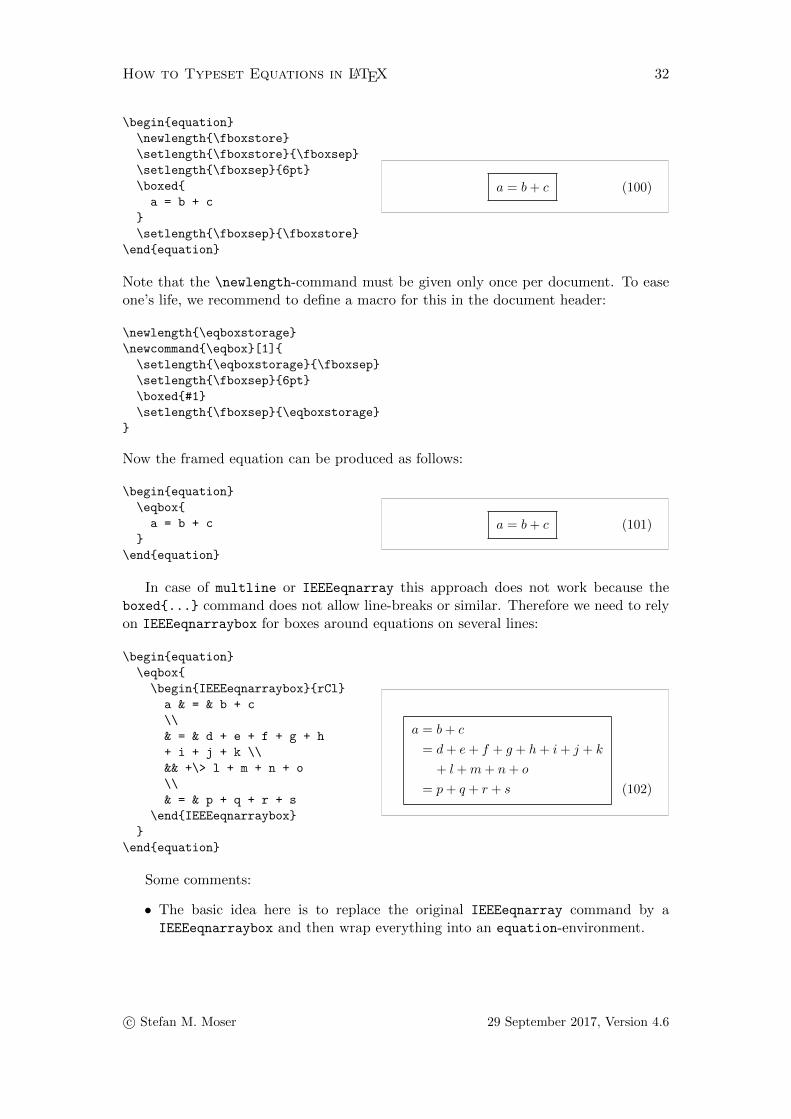
\begin{equation}
\newlength{\fboxstore}
\setlength{\fboxstore}{\fboxsep}
\setlength{\fboxsep}{6pt}
\boxed{
a = b + c
}
\setlength{\fboxsep}{\fboxstore}
\end{equation}
a = b+ c (100)
Note that the \newlength-command must be given only once per document. To easeone’s life, we recommend to define a macro for this in the document header:
\newlength{\eqboxstorage}
\newcommand{\eqbox}[1]{
\setlength{\eqboxstorage}{\fboxsep}
\setlength{\fboxsep}{6pt}
\boxed{#1}
\setlength{\fboxsep}{\eqboxstorage}
}
Now the framed equation can be produced as follows:
\begin{equation}
\eqbox{
a = b + c
}
\end{equation}
a = b+ c (101)
In case of multline or IEEEeqnarray this approach does not work because theboxed{...} command does not allow line-breaks or similar. Therefore we need to relyon IEEEeqnarraybox for boxes around equations on several lines:
\begin{equation}
\eqbox{
\begin{IEEEeqnarraybox}{rCl}
a & = & b + c
\\
& = & d + e + f + g + h
+ i + j + k \\
&& +\> l + m + n + o
\\
& = & p + q + r + s
\end{IEEEeqnarraybox}
}
\end{equation}
a = b+ c
= d+ e+ f + g + h+ i+ j + k
+ l +m+ n+ o
= p+ q + r + s (102)
Some comments:
• The basic idea here is to replace the original IEEEeqnarray command by aIEEEeqnarraybox and then wrap everything into an equation-environment.
c© Stefan M. Moser 29 September 2017, Version 4.6
How to Typeset Equations in LATEX 33
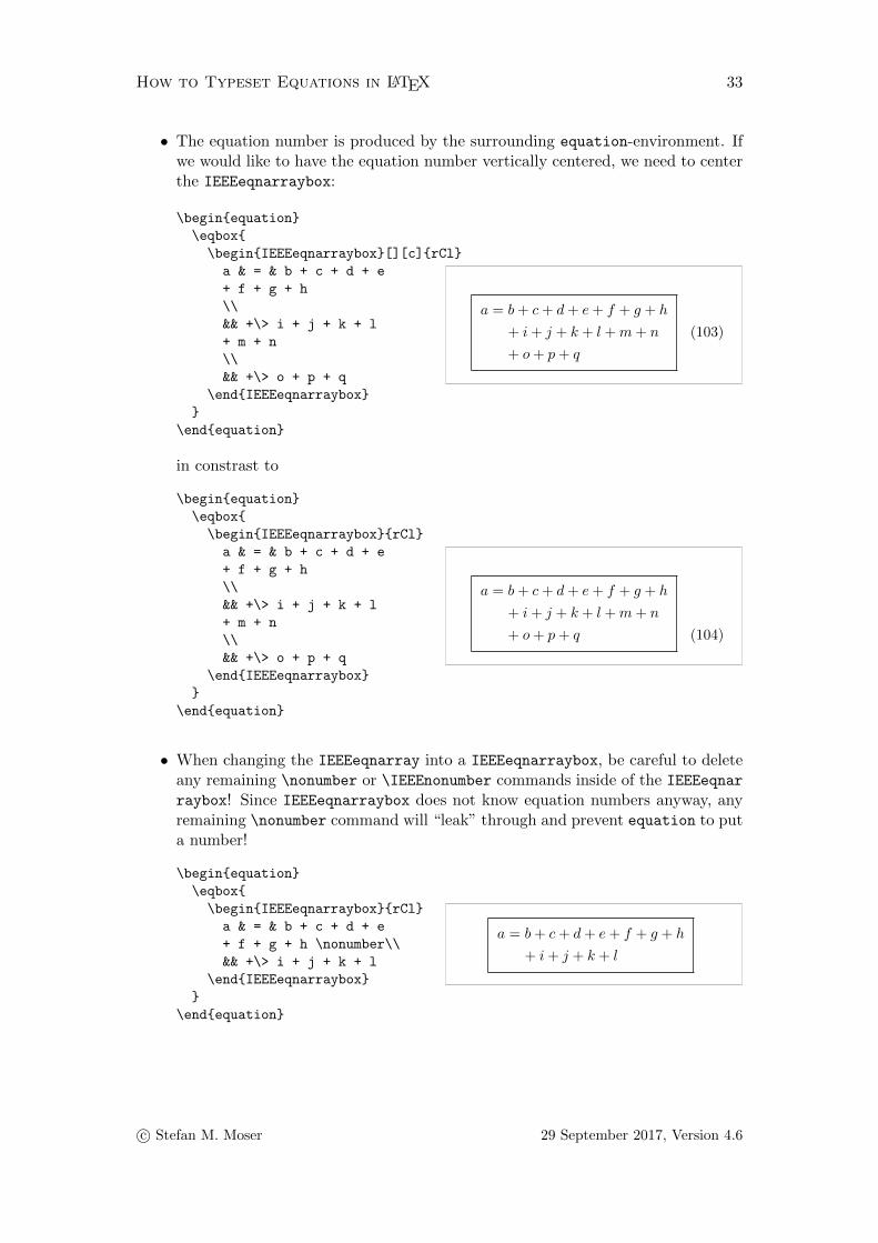
• The equation number is produced by the surrounding equation-environment. Ifwe would like to have the equation number vertically centered, we need to centerthe IEEEeqnarraybox:
\begin{equation}
\eqbox{
\begin{IEEEeqnarraybox}[][c]{rCl}
a & = & b + c + d + e
+ f + g + h
\\
&& +\> i + j + k + l
+ m + n
\\
&& +\> o + p + q
\end{IEEEeqnarraybox}
}
\end{equation}
a = b+ c+ d+ e+ f + g + h
+ i+ j + k + l +m+ n
+ o+ p+ q
(103)
in constrast to
\begin{equation}
\eqbox{
\begin{IEEEeqnarraybox}{rCl}
a & = & b + c + d + e
+ f + g + h
\\
&& +\> i + j + k + l
+ m + n
\\
&& +\> o + p + q
\end{IEEEeqnarraybox}
}
\end{equation}
a = b+ c+ d+ e+ f + g + h
+ i+ j + k + l +m+ n
+ o+ p+ q (104)
• When changing the IEEEeqnarray into a IEEEeqnarraybox, be careful to deleteany remaining \nonumber or \IEEEnonumber commands inside of the IEEEeqnar
raybox! Since IEEEeqnarraybox does not know equation numbers anyway, anyremaining \nonumber command will “leak” through and prevent equation to puta number!
\begin{equation}
\eqbox{
\begin{IEEEeqnarraybox}{rCl}
a & = & b + c + d + e
+ f + g + h \nonumber\\
&& +\> i + j + k + l
\end{IEEEeqnarraybox}
}
\end{equation}
a = b+ c+ d+ e+ f + g + h
+ i+ j + k + l
c© Stefan M. Moser 29 September 2017, Version 4.6

How to Typeset Equations in LATEX 34
6.8 Fancy frames
Fancier frames can be produced using the mdframed package. Use the following com-mands in the header of your document:21
\usepackage{tikz}
\usetikzlibrary{shadows} %defines shadows
\usepackage[framemethod=tikz]{mdframed}
Then we can produce all kinds of fancy frames. We start by defining a certain style(still in the header of your document):
\global\mdfdefinestyle{myboxstyle}{%
shadow=true,
linecolor=black,
shadowcolor=black,
shadowsize=6pt,
nobreak=false,
innertopmargin=10pt,
innerbottommargin=10pt,
leftmargin=5pt,
rightmargin=5pt,
needspace=1cm,
skipabove=10pt,
skipbelow=15pt,
middlelinewidth=1pt,
afterlastframe={\vspace{5pt}},
aftersingleframe={\vspace{5pt}},
tikzsetting={%
draw=black,
very thick}
}
These settings are quite self-explanatory. Just play around! Now we define differenttypes of framed boxes:
% framed box that allows page-breaks
\newmdenv[style=myboxstyle]{whitebox}
\newmdenv[style=myboxstyle,backgroundcolor=black!20]{graybox}
% framed box that CANNOT be broken at end of page
\newmdenv[style=myboxstyle,nobreak=true]{blockwhitebox}
\newmdenv[style=myboxstyle,backgroundcolor=black!20,nobreak=true]{blockgraybox}
% invisible box that CANNOT be broken at end of page
\newmdenv[nobreak=true,hidealllines=true]{blockbox}
As the name suggests, the graybox adds a gray background color into the box, while thebackground in whitebox remains white. Moreover, blockwhitebox creates the sameframed box as whitebox, but makes sure that whole box is typeset onto one singlepage, while the regular whitebox can be split onto two (or even more) pages.
21The mdframed-package should be loaded after amsthm.sty.
c© Stefan M. Moser 29 September 2017, Version 4.6
How to Typeset Equations in LATEX 35
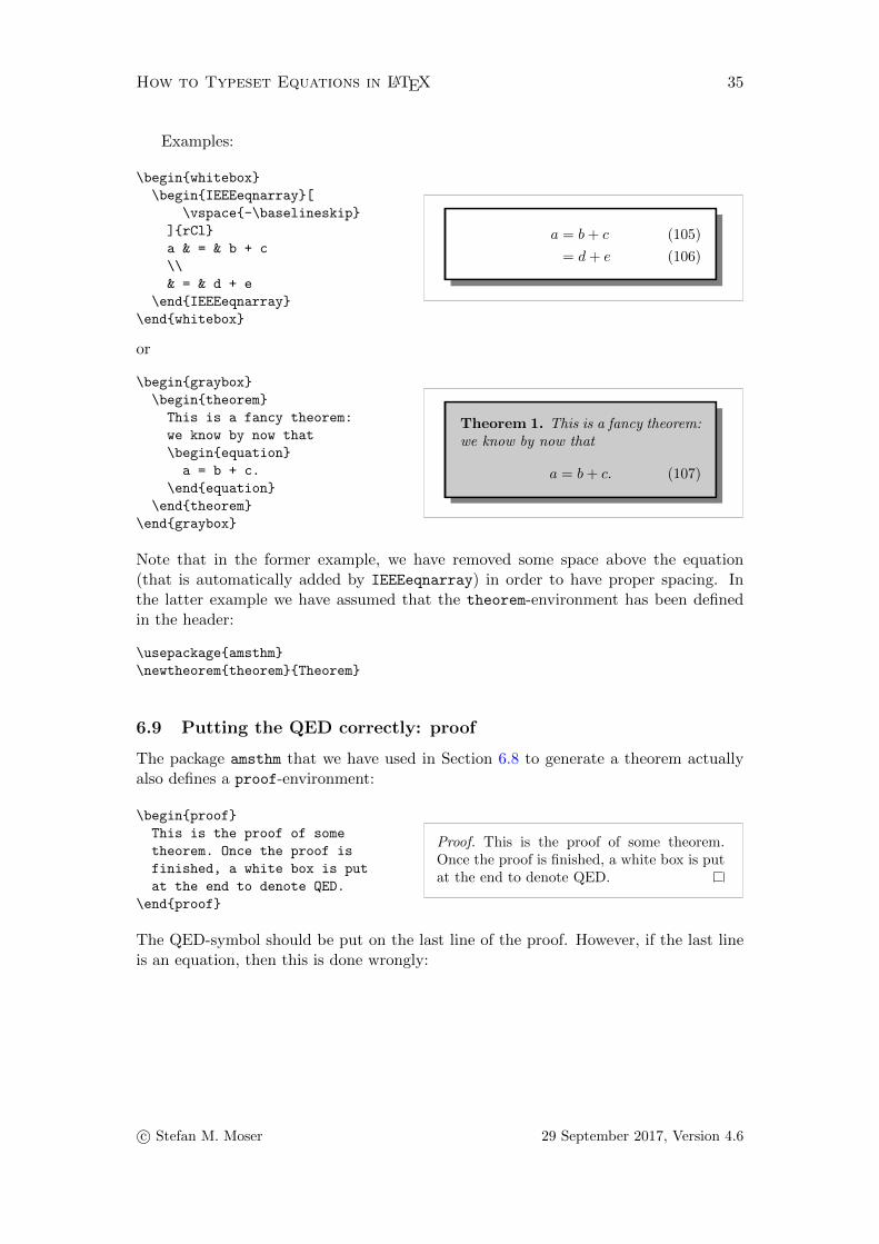
Examples:
\begin{whitebox}
\begin{IEEEeqnarray}[
\vspace{-\baselineskip}
]{rCl}
a & = & b + c
\\
& = & d + e
\end{IEEEeqnarray}
\end{whitebox}
a = b+ c (105)
= d+ e (106)
or
\begin{graybox}
\begin{theorem}
This is a fancy theorem:
we know by now that
\begin{equation}
a = b + c.
\end{equation}
\end{theorem}
\end{graybox}
Theorem 1. This is a fancy theorem:we know by now that
a = b+ c. (107)
Note that in the former example, we have removed some space above the equation(that is automatically added by IEEEeqnarray) in order to have proper spacing. Inthe latter example we have assumed that the theorem-environment has been definedin the header:
\usepackage{amsthm}
\newtheorem{theorem}{Theorem}
6.9 Putting the QED correctly: proof
The package amsthm that we have used in Section 6.8 to generate a theorem actuallyalso defines a proof-environment:
\begin{proof}
This is the proof of some
theorem. Once the proof is
finished, a white box is put
at the end to denote QED.
\end{proof}
Proof. This is the proof of some theorem.Once the proof is finished, a white box is putat the end to denote QED.
The QED-symbol should be put on the last line of the proof. However, if the last lineis an equation, then this is done wrongly:
c© Stefan M. Moser 29 September 2017, Version 4.6

How to Typeset Equations in LATEX 36
\begin{proof}
This is a proof that ends
with an equation: (bad)
\begin{equation*}
a = b + c.
\end{equation*}
\end{proof}
Proof. This is a proof that ends with an equa-tion: (bad)
a = b+ c.
In such a case, the QED-symbol must be put by hand using the command \qedhere:
\begin{proof}
This is a proof that ends
with an equation: (correct)
\begin{equation*}
a = b + c. \qedhere
\end{equation*}
\end{proof}
Proof. This is a proof that ends with an equa-tion: (correct)
a = b+ c.
Unfortunately, this correction does not work for IEEEeqnarray:
\begin{proof}
This is a proof that ends
with an equation array: (wrong)
\begin{IEEEeqnarray*}{rCl}
a & = & b + c \\
& = & d + e. \qedhere
\end{IEEEeqnarray*}
\end{proof}
Proof. This is a proof that ends with an equa-tion array: (wrong)
a = b+ c
= d+ e.
The reason for this is the internal structure of IEEEeqnarray: it always puts twoinvisible columns at both sides of the array that only contain a stretchable space.Thereby, IEEEeqnarray ensures that the equation array is horizontally centered. The\qedhere-command should actually be put outside this stretchable space, but this doesnot happen as these columns are invisible to the user.
Luckily, there is a very simple remedy: We explicitly define these stretching columnsourselves!
\begin{proof}
This is a proof that ends
with an equation array: (correct)
\begin{IEEEeqnarray*}{+rCl+x*}
a & = & b + c \\
& = & d + e. & \qedhere
\end{IEEEeqnarray*}
\end{proof}
Proof. This is a proof that ends with an equa-tion array: (correct)
a = b+ c
= d+ e.
Here, the + in {+rCl+x*} denotes a stretchable space, one on the left of the equations(which, if not specified, will be done automatically by IEEEeqnarray) and one on theright of the equations. But now on the right, after the stretching column, we addan empty column x. This column will only be needed on the last line for puttingthe \qedhere-command. Finally, we specify a *. This is a null-space that preventsIEEEeqnarray to add another unwanted +-space.
c© Stefan M. Moser 29 September 2017, Version 4.6
How to Typeset Equations in LATEX 37
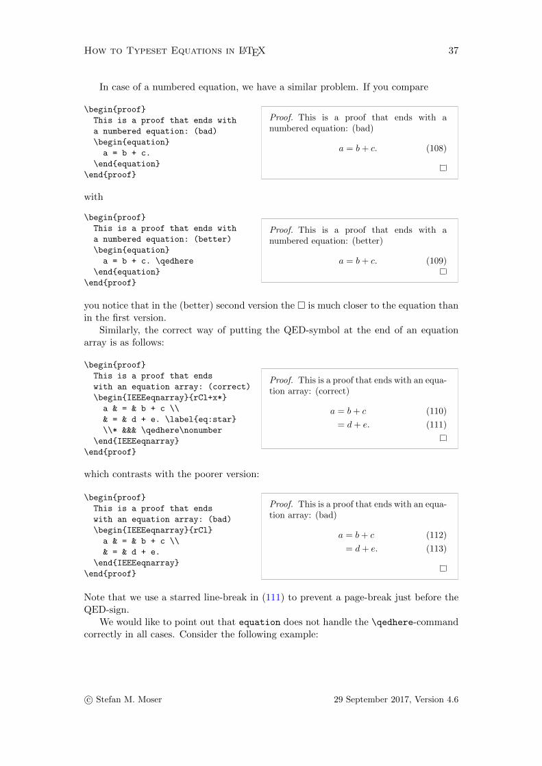
In case of a numbered equation, we have a similar problem. If you compare
\begin{proof}
This is a proof that ends with
a numbered equation: (bad)
\begin{equation}
a = b + c.
\end{equation}
\end{proof}
Proof. This is a proof that ends with anumbered equation: (bad)
a = b+ c. (108)
with
\begin{proof}
This is a proof that ends with
a numbered equation: (better)
\begin{equation}
a = b + c. \qedhere
\end{equation}
\end{proof}
Proof. This is a proof that ends with anumbered equation: (better)
a = b+ c. (109)
you notice that in the (better) second version the � is much closer to the equation thanin the first version.
Similarly, the correct way of putting the QED-symbol at the end of an equationarray is as follows:
\begin{proof}
This is a proof that ends
with an equation array: (correct)
\begin{IEEEeqnarray}{rCl+x*}
a & = & b + c \\
& = & d + e. \label{eq:star}
\\* &&& \qedhere\nonumber
\end{IEEEeqnarray}
\end{proof}
Proof. This is a proof that ends with an equa-tion array: (correct)
a = b+ c (110)
= d+ e. (111)
which contrasts with the poorer version:
\begin{proof}
This is a proof that ends
with an equation array: (bad)
\begin{IEEEeqnarray}{rCl}
a & = & b + c \\
& = & d + e.
\end{IEEEeqnarray}
\end{proof}
Proof. This is a proof that ends with an equa-tion array: (bad)
a = b+ c (112)
= d+ e. (113)
Note that we use a starred line-break in (111) to prevent a page-break just before theQED-sign.
We would like to point out that equation does not handle the \qedhere-commandcorrectly in all cases. Consider the following example:
c© Stefan M. Moser 29 September 2017, Version 4.6

How to Typeset Equations in LATEX 38
\begin{proof}
This is a bad example for the
usage of \verb+\qedhere+ in
combination with \verb+equation+:
\begin{equation}
a = \sum_{\substack{x_i\\
|x_i|>0}} f(x_i).
\qedhere
\end{equation}
\end{proof}
Proof. This is a bad example for the usage of\qedhere in combination with equation:
a =∑xi
|xi|>0
f(xi). (114)
A much better solution can be achieved with IEEEeqnarray:
\begin{proof}
This is the corrected example
using \verb+IEEEeqnarray+:
\begin{IEEEeqnarray}{c+x*}
a = \sum_{\substack{x_i\\
|x_i|>0}} f(x_i).
\\* & \qedhere\nonumber
\end{IEEEeqnarray}
\end{proof}
Proof. This is the corrected example usingIEEEeqnarray:
a =∑xi
|xi|>0
f(xi). (115)
Here, we add an additional line to the equation array without number, and put \qedherecommand there (within the additional empty column on the right). Note how the �in the bad example is far too close the equation number and is actually inside themathematical expression. A similar problem also occurs in the case of no equationnumber.
Hence:
We recommend not to use \qedhere in combination with equation, butexclusively with IEEEeqnarray.
6.10 Putting the QED correctly: IEEEproof
IEEEtrantools also provides its own proof-environment that is slightly more flexiblethan the proof of amsthm: IEEEproof. Note that under the IEEEtran-class, amsthm isnot permitted and therefore proof is not defined, i.e., one must use IEEEproof.
IEEEproof offers the command \IEEEQEDhere that produces the QED-symbol rightat the place where it is invoked and will switch off the QED-symbol at the end.
\begin{IEEEproof}
This is a short proof:
\begin{IEEEeqnarray}{rCl+x*}
a & = & b + c \\
& = & d+ e \label{eq:qed}
\\* &&& \nonumber\IEEEQEDhere
\end{IEEEeqnarray}
\end{IEEEproof}
Proof: This is a short proof:
a = b+ c (116)
= d+ e (117)
c© Stefan M. Moser 29 September 2017, Version 4.6

How to Typeset Equations in LATEX 39
So, in this sense \IEEEQEDhere plays the same role for IEEEproof as \qedhere forproof. Note, however, that their behavior is not exactly equivalent: \IEEEQEDhere
always puts the QED-symbol right at the place it is invoked and does not move it tothe end of the line. So, for example, inside of a list, an additional \hfill is needed:
\begin{IEEEproof}
A proof containing a list and
two QED-symbols:
\begin{enumerate}
\item Fact one.\IEEEQEDhere
\item Fact two.\hfill\IEEEQEDhere
\end{enumerate}
\end{IEEEproof}
Proof: A proof containing a list and twoQED-symbols:
1. Fact one.
2. Fact two.
Unfortunately, \hfill will not work inside an equation. To get the behavior of\qedhere there, one must use \IEEEQEDhereeqn instead:
\begin{IEEEproof}
Placed directly behind math:
\begin{equation*}
a = b + c. \hfill\IEEEQEDhere
\end{equation*}
Moved to the end of line:
\begin{equation*}
a = b + c. \IEEEQEDhereeqn
\end{equation*}
\end{IEEEproof}
Proof: Placed directly behind math:
a = b+ c.
Moved to the end of line:
a = b+ c.
\IEEEQEDhereeqn even works in situations with equation numbers, however, in contrastto \qedhere it does not move the QED-symbol to the next line, but puts it in front ofthe number:
\begin{IEEEproof}
Placed directly before the
equation number:
\begin{equation}
a = b + c. \IEEEQEDhereeqn
\end{equation}
With some additional spacing:
\begin{equation}
a = b + c. \IEEEQEDhereeqn\;
\end{equation}
\end{IEEEproof}
Proof: Placed directly before the equa-tion number:
a = b+ c. (118)
With some additional spacing:
a = b+ c. (119)
To get the behavior where the QED-symbol is moved to the next line, use the approachbased on IEEEeqnarray as shown in (117).
c© Stefan M. Moser 29 September 2017, Version 4.6

How to Typeset Equations in LATEX 40
Once again:
We recommend not to use \IEEEQEDhere and \IEEEQEDhereeqn in combinationwith equation, but to rely on \IEEEQEDhere and IEEEeqnarray exclusively.
Furthermore, IEEEproof offers the command \IEEEQEDoff to suppress the QED-symbol completely; it allows to change the QED-symbol to be an open box as inSection 6.9; and it allows to adapt the indentation of the proof header (default valueis 2\parindent). The latter two features are shown in the following example:
\renewcommand{\IEEEproofindentspace}{0em}
\renewcommand{\IEEEQED}{\IEEEQEDopen}
\begin{IEEEproof}
Proof without
indentation and an
open QED-symbol.
\end{IEEEproof}
Proof: Proof without indentation and anopen QED-symbol.
The default QED-symbol can be reactivated again by redefining \IEEEQED to be \IEEEQEDclosed.
We end this section by pointing out that IEEE standards do not allow a QED-symbol and an equation put onto the same line. Instead one should follow the example(117).
6.11 Double-column equations in a two-column layout
Many scientific publications are in a two-column layout in order to save space. Thismeans that the available width for the equations is considerably smaller than for a one-column layout and will cause correspondingly more line-breaks. Then the advantagesof the IEEEeqnarray-environment are even more pronounced.
However, there are very rare situations when the breaking of an equation into twoor more lines will result in a very poor typesetting, even if IEEEeqnarray with all itstricks is used. In such a case, a possible solution is to span an equation over bothcolumns. But the reader be warned:
Unless there is no other solution, we strongly discourage from the usage ofdouble-column equations in a two-column layout for aesthetic reasons and
because the LATEX code is rather ugly!
The trick is to use the figure-environment to create a floating object containingthe equation similarly to a included graphic. Concretely, we have to use figure* tocreate a float that stretches over both columns. Since in this way the object becomesfloating, the equation numbering has to be carefully taken care of.
We explain the details using an example. We start by defining two auxiliary equationcounters:
c© Stefan M. Moser 29 September 2017, Version 4.6
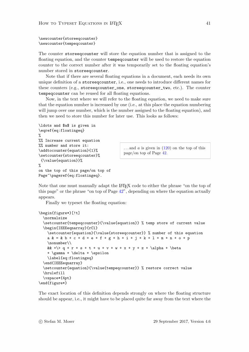
How to Typeset Equations in LATEX 41
\newcounter{storeeqcounter}
\newcounter{tempeqcounter}
The counter storeeqcounter will store the equation number that is assigned to thefloating equation, and the counter tempeqcounter will be used to restore the equationcounter to the correct number after it was temporarily set to the floating equation’snumber stored in storeeqcounter.
Note that if there are several floating equations in a document, each needs its ownunique definition of a storeeqcounter, i.e., one needs to introduce different names forthese counters (e.g., storeeqcounter_one, storeeqcounter_two, etc.). The countertempeqcounter can be reused for all floating equations.
Now, in the text where we will refer to the floating equation, we need to make surethat the equation number is increased by one (i.e., at this place the equation numberingwill jump over one number, which is the number assigned to the floating equation), andthen we need to store this number for later use. This looks as follows:
\ldots and $a$ is given in
\eqref{eq:floatingeq}
%
%% Increase current equation
%% number and store it:
\addtocounter{equation}{1}%
\setcounter{storeeqcounter}%
{\value{equation}}%
%
on the top of this page/on top of
Page~\pageref{eq:floatingeq}.
. . . and a is given in (120) on the top of thispage/on top of Page 42.
Note that one must manually adapt the LATEX code to either the phrase “on the top ofthis page” or the phrase “on top of Page 42”, depending on where the equation actuallyappears.
Finally we typeset the floating equation:
\begin{figure*}[!t]
\normalsize
\setcounter{tempeqcounter}{\value{equation}} % temp store of current value
\begin{IEEEeqnarray}{rCl}
\setcounter{equation}{\value{storeeqcounter}} % number of this equation
a & = & b + c + d + e + f + g + h + i + j + k + l + m + n + o + p
\nonumber\\
&& +\> q + r + s + t + u + v + w + x + y + z + \alpha + \beta
+ \gamma + \delta + \epsilon
\label{eq:floatingeq}
\end{IEEEeqnarray}
\setcounter{equation}{\value{tempeqcounter}} % restore correct value
\hrulefill
\vspace*{4pt}
\end{figure*}
The exact location of this definition depends strongly on where the floating structureshould be appear, i.e., it might have to be placed quite far away from the text where the
c© Stefan M. Moser 29 September 2017, Version 4.6

How to Typeset Equations in LATEX 42
a = b+ c+ d+ e+ f + g + h+ i+ j + k + l +m+ n+ o+ p
+ q + r + s+ t+ u+ v + w + x+ y + z + α+ β + γ + δ + ε (120)
equation is referred to.22 Note that this might need some trial and error, particularlyif there are other floating objects around to be placed by LATEX.
Be aware that due to a limitation of LATEX, double-column floating objects cannotbe placed at the bottom of pages, i.e., \begin{figure*}[!b] will not work correctly.This can be corrected if we include the following line in the header of our document:
\usepackage{stfloats}
However, this package is very invasive and might cause troubles with other packages.23
7 Emacs and IEEEeqnarray
When working with Emacs, you can ease your life by defining a few new commands.In the dot_emacs-file that comes together with this document the following commandsare defined:
• Control-c i: Insert an IEEEeqnarray-environment (similar to Control-c Control-e) with argument {rCl}.
• Control-c o: As Control-c i, but the *-version.
• Control-c b: Add a line-break at a specific place. This is very helpful in editingtoo long lines. Suppose you have typed the following LATEX code:
\begin{IEEEeqnarray}{rCl}
a & = & b + c \\
& = & d + e + f + g + h + i
+ j + k + l + m + n + o
\end{IEEEeqnarray}
a = b+ c (121)
= d+ e+ f + g + h+ i+ j + k + l +m+ n+ o(122)
After compiling you realize that you have to break the line before l. You nowjust have to put the cursor on the +-sign in front of l and press Control-c b.Then the line is wrapped there and also the additional space \> is added at theright place:
22It needs to be placed after the reference in the text, though, as otherwise the equation numberstored in storeeqcounter is not defined yet. This could again be fixed, but only if we set the equationnumber (i.e., storeeqcounter) manually (ugly!!).
23In particular, it cannot be used together with the package fixltx2e.sty. Luckily, the latter is notneeded anymore starting with TeXLive 2015.
c© Stefan M. Moser 29 September 2017, Version 4.6

How to Typeset Equations in LATEX 43
\begin{IEEEeqnarray}{rCl}
a & = & b + c \\
& = & d + e + f + g + h + i
+ j + k \nonumber\\
&& +\> l + m + n + o
\end{IEEEeqnarray}
a = b+ c (123)
= d+ e+ f + g + h+ i+ j + k
+ l +m+ n+ o (124)
• Control-c n: As Control-c b, but without adding the additional space \>.
• Control-c Control-b: Remove a line-break (undo of Control-c b and Control-c n). Position the cursor before the \nonumber and press Control-c Control-b.
• Control-c m: Insert a \IEEEeqnarraymulticol-command. This is very helpfulwhen the LHS is too long. Suppose you have typed the following LATEX code:
\begin{IEEEeqnarray}{rCl}
a + b + c + d + e + f
+ g + h + i + j
& = & k + l \\
& = & m + n
\end{IEEEeqnarray}
a+ b+ c+ d+ e+ f + g + h+ i+ j = k + l(125)
= m+ n(126)
After compiling you realize that the LHS is too long. You now just have to putthe cursor somewhere on the first line and type Control-c m. Then you get
\begin{IEEEeqnarray}{rCl}
\IEEEeqnarraymulticol{3}{l}{
a + b + c + d + e + f
+ g + h + i + j
}\nonumber \\ \quad
& = & k + l \\
& = & m + n
\end{IEEEeqnarray}
a+ b+ c+ d+ e+ f + g + h+ i+ j
= k + l (127)
= m+ n (128)
• Finally, in the dot_emacs-file, settings are given that make IEEEeqnarray andIEEEeqnarraybox known to Emacs’ LATEX-mode, reftex, and ispell. This waymany standard Emacs commands can be used as usual also in the context ofIEEEeqnarray. For example, Control-c ( will add an equation label.
8 Some Useful Definitions
There are a couple of mathematical symbols that cannot easily be found in LATEX-symbol collections. In the following, a few such symbols are listed and a possible wayis proposed of how to define them.
• Markov Chains: One of the existing customary ways to describe that three ran-dom variables form a Markov chain is
\begin{equation*}
X \markov Y \markov Z
\end{equation*}X (−− Y (−− Z
c© Stefan M. Moser 29 September 2017, Version 4.6

How to Typeset Equations in LATEX 44
Here, the symbol ’(−−’ is defined as a combination of \multimap (() and twominus-signs (−):
\newcommand{\markov}{\mathrel{\multimap}\joinrel\mathrel{-}%
\joinrel\mathrel{\mkern-6mu}\joinrel\mathrel{-}}
For this definition to work, beside amsmath also the package amssymb needs to beloaded.
• Independence: To describe that two random variables are statistically independ-ent, I personally prefer the following symbol:
\begin{equation*}
X \indep Y
\end{equation*}X ⊥⊥ Y
Accordingly,
\begin{equation*}
X \dep Y
\end{equation*}X 6⊥⊥ Y
denotes that X and Y are not statistically independent.
These two symbols are created by two \bot (⊥) signs:
\newcommand{\indep}{\mathrel{\bot}\joinrel\mathrel{\mkern-5mu}%
\joinrel\mathrel{\bot}}
\newcommand{\dep}{\centernot\indep}
For this definition to work, beside amsmath also the package centernot needs tobe loaded.
• Integration-d: The d in an integral is not a variable, but rather an operator. Ittherefore should not be typeset italic d, but Roman d. Moreover, there should bea small spacing before the operator:
\begin{equation*}
\int_a^b f(x) \dd x = \int_a^b
\ln\left(\frac{x}{2}\right)
\dd x
\end{equation*}
∫ b
a
f(x) dx =
∫ b
a
ln(x
2
)dx
To make sure that this spacing always works out correctly, I recommend thefollowing definition:
\newcommand{\dd}{\mathop{}\!\mathrm{d}}
c© Stefan M. Moser 29 September 2017, Version 4.6

9 Some Final Remarks and Acknowledgments
The “rules” stated in this document are purely based on my own experience withtypesetting LATEX in my publications and on my — some people might say unfortunate— habit of incorporating many mathematical expressions in there.
If you encounter any situation that seems to contradict the suggestions of thisdocument, then I would be very happy if you could send me a corresponding LATEX orPDF file. As a matter of fact, any kind of feedback, criticism, suggestion, etc. is highlyappreciated! Write to
Thanks!I would like to mention that during the writing and updating of this document
I profited tremendously from the help of Michael Shell, the author of IEEEtran. Hewas always available for explanations when I got stuck somewhere. Moreover, I grate-fully acknowledge the comments from (in alphabetical order) Helmut Bolcskei, AmosLapidoth, Edward Ross, Omar Scaglione, and Sergio Verdu.
Stefan M. Moser
Index
\\∗, 14, 25
.emacs, 3, 42
$$, 3
adapting bracket-size, 28
align, 7
aligning across blocks, 20
amsmath, 3, 44
amssymb, 44
amsthm, 34, 35
array, 21
bigl-bigr, 29, 30
binary sign, 14
blockbox, 34
blockgraybox, 34
blockwhitebox, 34
Bmatrix, 28
bmatrix, 28
boxed, 31
brackets, 24
adapting size, 28
case distinction, 21, 23
cases, 23
individual numbers, 24
centernot, 44
dd, 44
dependence, 44
displaymath, 3
dot emacs, 3, 42
double-column equations, 40
Emacs, 42
eqbox, 32
45

How to Typeset Equations in LATEX 46
eqnarray, 9equation, 3, 10
floating, 40wrapping, 4
equation numbers, 16italic or bold, 11outside of boundary, 13
fancy frames, 34fboxsep, 31figure, 40fixltx2e, 42framed equations, 31
breakable, 34fancy, 34
graybox, 34grouping equations, 24
hyperlinks, 18block of subequations, 19
hyperref, 18
IEEEeqnarray, 10align across blocks, 20page-breaks, 20replacing equation, 10replacing multline, 12
IEEEeqnarraybox, 21, 22IEEEeqnarrayboxm, 21IEEEeqnarrayboxt, 21IEEEeqnarraymulticol, 13, 18IEEEeqnarraynumspace, 12IEEEeqnarraystrutmode, 22IEEEeqnarraystrutsizeadd, 23IEEElabelanchoreqn, 19IEEEnonumber, 16IEEEnosubnumber, 16IEEEproof, 38IEEEQEDclosed, 40IEEEQEDhere, 38IEEEQEDhereeqn, 39, 40IEEEQEDoff, 40IEEEQEDopen, 40IEEEstrut, 21, 26
IEEEtrantools, 9IEEEyesnumber, 16IEEEyessubnumber, 16independence, 44integration-d, 44interdisplaylinepenalty, 20
jot, 25
labelsplacing, 18
left, 28left-right, 28
line-break, 30lefteqn, 9, 13LHS
too long, 13too long, RHS too short, 6
line-break, 14, 30
markov, 44Markov chain, 43matrices, 28matrix, 28mdframed, 34middle, 29mleftright, 29multline, 4, 6, 10
noalign, 20nonumber, 16normalbaselineskip, 28numbers, 16numcases, 24
page-breaks, 20phantom, 31pmatrix, 28proof, 35
QEDIEEEproof, 38proof, 35
qedhere, 36
c© Stefan M. Moser 29 September 2017, Version 4.6

How to Typeset Equations in LATEX 47
equation, 38
IEEEeqnarray, 36
reference to subequations, 19
RHS
slightly too long, 12
too short, LHS too long, 6
right, 28
shift to the left, 12
single equation, 3
too long, 4
sizecorr, 31
smash, 25
spacing, 21
stfloats, 42
storeeqcounter, 40
subequations, 19
subnumberinglabel, 19
subnumbers, 16
subnumcases, 24symbols
dependence, 44independence, 44integration-d, 44Markov chain, 43
table, 21, 22tabular, 21tempeqcounter, 40theorem, 35
unary sign, 14
vertical spacing, 21Vmatrix, 28vmatrix, 28
whitebox, 34wrapping, 4
c© Stefan M. Moser 29 September 2017, Version 4.6