highly efficient maximum power point tracking using a quasi-double-boost dc/dc converter for
TRANSCRIPT

University of Nebraska - LincolnDigitalCommons@University of Nebraska - LincolnTheses, Dissertations, and Student Research fromElectrical & Computer Engineering Electrical & Computer Engineering, Department of
Winter 12-2-2011
Highly Efficient Maximum Power Point TrackingUsing a Quasi-Double-Boost DC/DC Converterfor Photovoltaic SystemsChristopher J. LohmeierUniversity of Nebraska-Lincoln, [email protected]
Follow this and additional works at: http://digitalcommons.unl.edu/elecengtheses
Part of the Controls and Control Theory Commons, Electrical and Electronics Commons, Powerand Energy Commons, and the Signal Processing Commons
This Article is brought to you for free and open access by the Electrical & Computer Engineering, Department of at DigitalCommons@University ofNebraska - Lincoln. It has been accepted for inclusion in Theses, Dissertations, and Student Research from Electrical & Computer Engineering by anauthorized administrator of DigitalCommons@University of Nebraska - Lincoln.
Lohmeier, Christopher J., "Highly Efficient Maximum Power Point Tracking Using a Quasi-Double-Boost DC/DC Converter forPhotovoltaic Systems" (2011). Theses, Dissertations, and Student Research from Electrical & Computer Engineering. 32.http://digitalcommons.unl.edu/elecengtheses/32

Highly Efficient Maximum Power Point
Tracking Using a Quasi-Double-Boost DC/DC
Converter for Photovoltaic Systems
By
Christopher J. Lohmeier
Presented to the Faculty of
The Graduate College at the University of Nebraska
In Partial Fulfillment of Requirements
For the Degree of Master of Science
Major: Electrical Engineering
Under the Supervision of Professor Wei Qiao
Lincoln, NE
December, 2011

Highly Efficient Maximum Power Point Tracking Using a Quasi-Double-Boost
DC/DC Converter for Photovoltaic Systems
Christopher John Lohmeier, M.S.
University of Nebraska, 2011
Adviser: Wei Qiao
Solar photovoltaic (PV) panels are a great source of renewable energy
generation. The biggest problem with solar systems is relatively low efficiency and high
cost. This work hopes to alleviate this problem by using novel power electronic
converter and control designs. An electronic DC/DC converter, called “Quasi-Double-
Boost DC/DC Converter,” is designed for a Solar PV system. A Maximum Power Point
Tracking (MTTP) algorithm is implemented through this converter. This algorithm allows
the PV system to work at its highest efficiency. Different current sensing and sensorless
technologies used with the converter for the MPPT algorithm are offered and tested.
Design aspects of the system and components will be discussed. Results from
simulations and experiments will be presented. These results will show that the
proposed converter and MPPT control algorithm improves overall PV system efficiency
without adding much additional cost.

iii
Table of Contents
List of Figures ...................................................................................................................... vi
List of Tables ..................................................................................................................... viii
Chapter 1: Introduction ..................................................................................................... 1
Chapter 2: System Configuration ....................................................................................... 5
System Layout ................................................................................................................ 5
The PV Panel ................................................................................................................... 5
Modeling of the PV Panel ............................................................................................... 8
The Quasi-Double-Boost DC/DC Converter .................................................................... 9
Chapter 3: The Maximum Power Point Tracking Algorithm ............................................ 14
Why is it needed? ......................................................................................................... 14
How does it work? ........................................................................................................ 16
The MPPT Algorithm .................................................................................................... 17
Chapter 4: Voltage and Current Sensing Technologies for MPPT Control ...................... 22
Traditional Sensing Technology .................................................................................... 22
Current Sensorless Technology .................................................................................... 23
Inductor Current Sensing Technology .......................................................................... 26
Chapter 5: Simulation Results .......................................................................................... 30
Validation of the PV Panel Model ................................................................................ 30

iv
The Quasi-Double-Boost DC/DC Converter .................................................................. 31
The MPPT Control......................................................................................................... 34
Current-Sensorless MPPT Control ................................................................................ 38
Inductor Current Sensing Technology .......................................................................... 40
Sensing Technology Comparisons ................................................................................ 45
Chapter 6: Experimental Results ...................................................................................... 48
The Quasi-Double-Boost DC/DC Converter .................................................................. 49
The MPPT Control......................................................................................................... 56
Current-Sensorless MPPT Control ................................................................................ 64
Chapter 7: Conclusions, Contributions, and Recommendation for Future Work ........... 67
Bibliography ...................................................................................................................... 68
Appendix 1 - BP Solar Panel Model SX 3175 ..................................................................... 71
Appendix 2 - MATLAB Simulink Models ............................................................................ 73
The PV Panel Model ..................................................................................................... 73
The Converter Model ................................................................................................... 74
The MPPT Control Block ............................................................................................... 75
The MPPT Code ............................................................................................................ 76
Code for Artificial Neural Network ............................................................................... 77
Code to Test the Results of Training the Artificial Neural Network ............................. 79

v
Appendix 3 - MPPT Code Implemented in the Arduino ................................................... 80
Appendix 4 - LabVIEW Data Acquisition System............................................................... 83

vi
List of Figures
Figure 1. The layout of the overall PV system. ................................................................... 5
Figure 2. A representative I-V curve for a solar cell showing the MPP (Wenham, 2009). . 6
Figure 3. The PV panel model. ............................................................................................ 8
Figure 4. The current waveform in DCM mode. ............................................................... 10
Figure 5. Flowchart of the P&O MPPT algorithm. ............................................................ 19
Figure 6. Block diagram of the proposed current-sensorless control system. ................. 23
Figure 7. Voltage and current waveforms in CCM. ........................................................... 24
Figure 8. The schematic of the sampling circuit for voltage ripple detection. ................ 26
Figure 9. Block diagram of the proposed inductor current sensing control system. ....... 27
Figure 10. Layout of the artificial neural network for inductor current estimation......... 28
Figure 11. I-V curves at different levels of solar irradiance generated by the PV panel
model. ............................................................................................................. 30
Figure 12. I-V curves at different levels of solar cell temperatures generated by the PV
panel model. ................................................................................................... 31
Figure 13. The inductor current of the converter in DCM and CCM. ............................... 33
Figure 14. Comparison of the calculated and simulated results of voltage regulation for
the DC/DC converter. ...................................................................................... 34
Figure 15. Simulation results of the MPPT control algorithm. ........................................ 36
Figure 16. The power estimation results. ......................................................................... 39
Figure 17. The MPPT results of the PV system. ................................................................ 40
Figure 18. Mean square error output during the neural network training. ..................... 41

vii
Figure 19. Comparison of actual and estimated input current. ....................................... 43
Figure 20. Simulation results of the inductor sensing MPPT control algorithm.............. 45
Figure 21. The experimental system. ............................................................................... 48
Figure 22. Observations from the converter being ran at a 50% duty cycle. .................. 49
Figure 23. Observations from the converter being ran at a 55% duty cycle. .................. 50
Figure 24. Observations from the converter being ran at a 60% duty cycle. .................. 50
Figure 25. Calculated, simulated, and experimental results of voltage regulation. ........ 52
Figure 26. The efficiency of the quasi-double-boost DC/DC converter. .......................... 55
Figure 27. Comparison of the power output of the PV panel with the proposed converter
and MPPT control system with the PV panel connected directly to a fixed
resistance on a cloudy day. .............................................................................. 59
Figure 28. Comparison of the power output of the PV panel with the proposed
converter and MPPT control system with the PV panel connected directly to a
fixed resistance at sunset. ................................................................................ 61
Figure 29. MPPT Comparison of the power output of the PV panel with the proposed
converter and MPPT control system with the PV panel connected directly to a
fixed resistance over a full sunny day. ............................................................. 63
Figure 30. The current estimation results. ....................................................................... 64
Figure 31. The MPPT result in high radiation (sunny) conditions. ................................... 65
Figure 32. The MPPT results in low radiation (cloudy) conditions. ................................. 65

viii
List of Tables
Table 1. Simulated and experimental input and output voltage values. ......................... 53
Table 2. Results of the converter efficiency test. ............................................................ 56

1
Chapter 1: Introduction
The past few years have been filled with news of fuel price hikes, oil spills, and
concerns of global warming. One of the few positives that can be taken from this is that
it is changing the average person’s mindset towards renewable energy. People are
finding the benefits of having their own renewable energy system more attractive than
they ever have before. The biggest form of renewable energy to benefit from this is
solar PV systems because of their many merits, such as cleanness and relative lack of
noise or movement, as well as their ease of installation and integration when compared
to wind turbines. However, the output power of a PV panel is largely determined by the
solar irradiation and the temperature of the panel. At a certain weather condition, the
output power of a PV panel depends on the terminal voltage of the system. To
maximize the power output of the PV system, a high-efficiency, low-cost DC/DC
converter with an appropriate maximum power point tracking (MPPT) algorithm is
commonly employed to control the terminal voltage of the PV system at optimal values
in various solar radiation conditions.
There are three main DC/DC converter technologies used with most PV systems
(Bernardo, 2009; Morales-Saldaña, 2006; Mrabti, 2009; Nabulsi, 2009; Shanthi, 2007).
The first of these converters is the buck converter (Bernardo, 2009; Mrabti, 2009). Buck
converters are step-down converters that output a voltage lower than the voltage that
is input to the converter. The standard buck converter has an output that is equivalent
to the input voltage multiplied by the duty cycle or

2
= ∗ (1-1)
Buck converters work for low voltage applications. They can be implemented in
MPPT algorithms (Bernardo, 2009), as long as the PV panels output voltage is greater
than the voltage required by the load. To maximize the efficiency of the PV panel from
near zero to the maximum output, the entire range of the duty cycle needs to be used
for the implementation of the MPPT algorithm.
The second commonly used converter in PV systems is a boost converter
(Shanthi, 2007). Boost converters are step-up converters that output a voltage higher
than the voltage that is input to the converter. The standard boost converter has an
output that is equivalent to the input voltage divided by the duty cycle.
=
(1-2)
Basic boost converters work well with the MPPT control as long as the load can
accept a voltage from the minimum output of the PV panel all the way up a certain
value (e.g., 5 times) subject to practical limits of the duty cycle (e.g., 80%). However, in
many applications, a high boost ratio is required for the DC/DC converter to connect the
low-voltage PV panel to a relatively high-voltage load or power grid. This cannot be
satisfied by using basic boost converters.
The third commonly used converter in solar PV systems is a cascaded boost
converter (Morales-Saldaña, 2006; Nabulsi, 2009). Cascaded boost converters have an

3
output that is equivalent to the input voltage divided by the duty cycle to the nth
power,
where n refers to the number of boost converters that are cascaded.
=
(1-3)
Cascaded boost converters work well in applications that require high voltage
boost ratios. One problem with both the boost and the cascaded boost converters is
the oscillations and relative instability under changing and startup conditions as shown
in (Rensburg, 2008).
In order to utilize the potential with any of these converters in a PV system, the
converter needs to be controlled by a MPPT algorithm. Various MPPT algorithms (Hua,
1998; Hussein, 1995; Koutroulis, 2001; Pan, 1999) have been proposed based on power
measurements, including the hill-climbing (HC) method (Koutroulis, 2001), perturb-and-
observe (P&O) method (Hua, 1998), and incremental conductance (IncCond) method
(Hussein, 1995). The HC and P&O methods achieve the same fundamental thought in
different ways (Salas, 2006). These two algorithms are widely used because of their
simplicity; however they can fail under rapidly changing atmospheric conditions. The
incremental conductance method can track the maximum power point (MPP) more
accurately than the HC and P&O algorithms can, however it is relatively complicated to
implement.
Every addition, converter and MPPT algorithm add additional cost to the entire
PV system. However the cost in minimal compared to the PV panels and can usually be
offset by improved efficiency. Improving efficiency is the easiest way to cut cost with a

4
PV system. A good MPPT algorithm and a high efficiency converter are a must to
improve efficiency but should not be the only changes to the standard setup. One
should also employ higher output voltages to lower line losses and allow for more
efficient AC conversion. The second easiest way to improve overall system cost is in the
components themselves. A higher and more stable line voltage will mean smaller AC
inverters with grid tie systems that will not need any boosting capabilities at all. The
removal of expensive components such as current sensors also helps to keep cost at a
minimum and improves the system reliability. The system needs to be robust enough
that when the consumer wants to expand their energy production by adding more
panels, they don’t need to replace their entire system. The DC/DC converter and MPPT
control algorithm proposed in this work will implement all of these improvements in
hopes creating a highly efficient, low-cost, and highly reliable solar PV system for clean
and renewable power generation.

5
Chapter 2: System Configuration
System Layout
The overall PV system layout can be seen in Figure 1. The system consists of a
PV panel or panels, a quasi-double-boost DC/DC converter, a MPPT control algorithm
and some sort of load.
Figure 1. The layout of the overall PV system.
The PV Panel
PV panels generate electricity through what is called the “Photovoltaic Effect”
(Wenham, 2009). In the simplest form the Photovoltaic Effect can be described as
follows: Light particles called photons are constantly emitted from the Sun. This can be
seen by the brightness on a sunny day when many of these particles make it to earth’s
surface. The effect comes into play when these particles hit a PV material, such as a
6
solar cell. When the photons impact this material it excites the atoms within the
material, which causes an electron-hole pair to form. A band gap built into the material
causes the electron to move along a certain predefined path. This electron-hole pair
creation happens many times over, throughout the panel. All of these flowing electrons
generate a current that is directed out of the panel to some type of load. Thus, the
photovoltaic effect converts light into the more useful form of power, electricity.
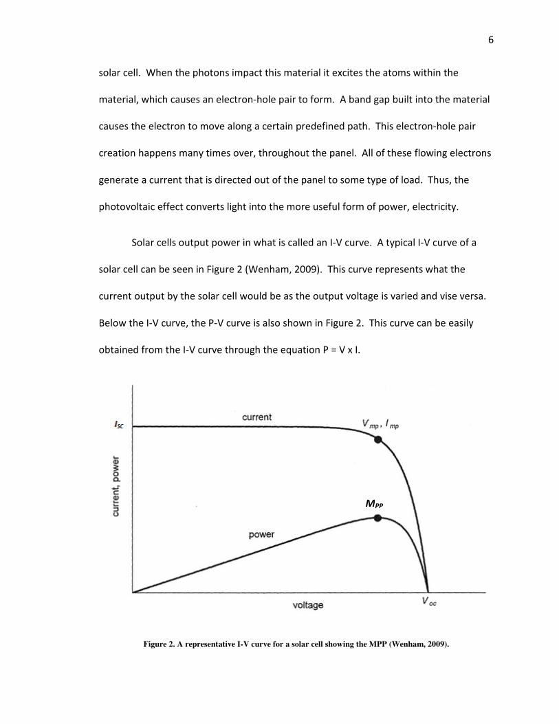
Solar cells output power in what is called an I-V curve. A typical I-V curve of a
solar cell can be seen in Figure 2 (Wenham, 2009). This curve represents what the
current output by the solar cell would be as the output voltage is varied and vise versa.
Below the I-V curve, the P-V curve is also shown in Figure 2. This curve can be easily
obtained from the I-V curve through the equation P = V x I.
Figure 2. A representative I-V curve for a solar cell showing the MPP (Wenham, 2009).
MPP

7
There are three other important aspects of a solar cell also shown in Figure 2.
The first two are the open circuit voltage (Voc) and the short circuit current (Isc) of the
cell. The open circuit voltage is the voltage that is output to the cell terminals when the
cell is exposed to light and there is no current flowing between the terminals. This is
also the maximum voltage that can be produced by the cell, which makes knowing this
number useful when designing a circuit or load to connect to the cell terminals. The
short circuit current is the current that will flow when the cell is under light and the
terminals are shorted together. This is the maximum current that can be output by the
specific solar cell. The third important aspect of a solar cell is the MPP. This is the point
where the cell is operating at maximum efficiency and outputting the highest power
available. The MPP also has voltage at maximum power (Vmp) and current at maximum
power (Imp) points associated with it. The way these points move and change with the
environmental conditions around the cell will be discussed in more detail later.
Each individual cell is relatively little in size and can only produce a small amount
of power. The Voc of an individual solar cell is usually approximately 0.6 V(Wenham,
2009). The cells become much more useful when combined in an array to create a PV
panel. When connected together the cells properties add together to create an I-V
curve that has the same appearance as that of an individual cell but is larger in
magnitude. The cells in an array are usually connected in series to obtain a higher and
more appropriate terminal voltage.

8
The PV panels used in this research are BP Solar model SX 3175 (Appendix 1).
Each panel consists of 72 individual solar cells connected in series to obtain a rated
power of 175 W, which corresponds to a maximum power current and voltage of 4.85 A
and 36.1 V, respectively. The panel has an open circuit voltage of 43.6 V and a short
circuit current of 5.3 A.
Modeling of the PV Panel
Figure 3. The PV panel model.
A PV panel model is developed using the work in (Tsai, 2008) as a starting point.
The panel is modeled as a current source as shown in Figure 3 that follows equation 2-1.
)1/)((exp)( −⋅+= − kTARiVqIIi SinTSph (2-1)
where i is the PV panel output current; Iph is photocurrent; IS(T) is the reverse saturation
current; q ( = 1.6×10⁻¹⁹
) is an electron charge; Vin is the terminal voltage of the PV panel;
RS is the PV panel series resistance; A is the ideal factor of the PN junction of the PV

9
diode, which varies in the range of [1, 2]; and k ( = 1.38×10⁻²³
J/K ) is the Boltzmann
constant. The photo current is then found using equation 2-2.
λ⋅−+=
)(
refTT
iK
scII ph (2-2)
where ISC is the short circuit current provided by the PV panel at a reference
temperature and an irradiance of 1kW/m2; Ki ( = 3mA/) is the temperature coefficient,
λ is the solar irradiance in kW/m2; and T and Tref are measured temperature and
reference temperature, respectively. The output current is then
)(exp)()( refSrefSS TTKTITI −= (2-3)
where IS(Tref) is the reverse saturation current (Tref = 295K) and Ks ( ≈ 0.072/) is the
temperature coefficient of the PV panel.
The Quasi-Double-Boost DC/DC Converter
Many DC/DC converter topologies were considered prior to designing the
system. Ultimately a double-boost DC/DC converter (Rensburg, 2008) was chosen
because of the requirement for a high voltage regulation ratio (200/28) as well as the
converter’s output stability over the entire duty cycle range. As shown in Figure 1, the
double-boost DC/DC converter consists of two inductors, two switches and three
diodes. The boost function is achieved by switching the two switches simultaneously.
However, the following analysis reveals that the voltage regulation ratio is not exactly
double boost previously derived (Rensburg, 2008).

10
Figure 4. The current waveform in DCM mode.
The converter can work in a continuous current mode (CCM) or a discontinuous
current mode (DCM). The DCM is studied since the CCM is a special case of the DCM.
The waveforms in the DCM are shown in Figure 4, where S1 and S2 are the gate signals of
the two switches; TS and D are the switching period and duty ratio of the DC/DC
converter, respectively; tc is the duration that the inductor currents decrease to zero
from the maximum value; and IM is the maximum inductor current. Neglecting the
ripples of vin and vout, the following formula can be obtained for the switch on and off
periods, respectively.
in S
M
V DTI
L= (2-4)
2 M
in out
c
IV V L
t− = − (2-5)
where L1 = L2 = L; Vin and Vout are the average values of vin and vout, respectively. Then
the voltage regulation ratio can be obtained from (2-4) and (2-5) as follows.

11
c
c
in
out
t
tDT
V
V +=
2 (2-6)
The average value of the input current I in a period can be calculated as:
2
c
M
S
tI D I
T
= +
(2-7)
According to the power conservation law, Vin*I = Pout, then
M
S
cin
outoutI
T
tDV
R
VV)
2( +=
× (2-8)
where R is the equivalent resistance of the load. Substituting (2-4) and (2-7) into (2-8),
then
L
RTD
T
t
T
t
T
tD
S
S
c
S
c
S
c
⋅⋅=
×
+
22
2 (2-9)
The conduction time tc can be derived from (2-9).
++
=
L
RD
L
R
STD
tc
2411 (2-10)
Equation (2-10) indicates that the conduction time during the switch off period is
related with R, L, T, and D. The following formula can be obtained by substituting (2-10)
into (2-6).

12
2
2411
++
=L
R
STD
V
V
in
out (2-11)
Equation (2-11) indicates that in the DCM, the voltage ratio is not only
determined by the duty ratio, but also determined by the output current and the
inductance value. If the equivalent load resistance varies from time to time, the duty
ratio should be changed to sustain the desired voltage gain.
When tc = (1−D) TS, the converter works in the critical mode, substituting tc into
(2-9), then the critical inductance LC is:
2)1(
2)1( S
C
RTDDL
D⋅
−=
+ (2-12)
Equation (2-12) indicates that the critical inductance depends on the duty cycle
and load. Equation (2-12) also indicates that there exist a supremum (i.e., the least
upper bound) value LM such that for any L > LM, the circuit will work in the CCM for any
duty ratios. This unique maximal critical inductance can be derived by setting the first
derivative of LC with respect to D as zero.
0=∂
∂
D
LC (2-13)
Then
2
113.0RT
LM ⋅= (2-14)

13
Therefore, (2-14) can be used to design the inductor so that the circuit always
works in the CCM when the load is fixed. On the other hand, if the inductance is fixed,
then there exists a critical duty cycle (DC), when D < DC, the converter works in the DCM;
otherwise, the converter works in the CCM, in which (2-6) can be further simplified as:
D
D
V
V
in
out
−
+=
1
1 (2-15)
Equation (2-15) indicates that the voltage regulation ratio is not simply twice
that of the basic boost converter as claimed in (Rensburg, 2008). Thus, the original
double-boost converter named in (Rensburg, 2008) is called the quasi-double-boost
converter from here on.

14
Chapter 3: The Maximum Power Point Tracking Algorithm
Why is it needed?
The I-V output curve characteristic of a PV panel is previously presented.
Associated with this curve is a MPP. This is the point where the solar cell is most
efficient in converting the solar energy into electrical energy. The MPP is not a fixed
point, it actually moves throughout the day. There are many factors that influence
where this point is at a given time.
The largest influence is the amount of solar radiation hitting the panel. The
more solar radiation that comes into contact with the panel the higher the Power curve,
in Figure 2 becomes; the less radiation the lower it becomes. This increase (or decrease)
in solar radiation also causes the MPP to sway back and forth as conditions change.
A variation in solar radiation over time is a factor that affects all PV panels no
matter where they are installed. The change can be caused by movement of the sun in
the sky relative to the PV panel. The greater the angle between the sun and the face of
the panel the lower the amount of radiation the panel receives. The movement of the
sun is very predictable and can even be accounted for through the use of other
mechanical solar tracking methods (Wenham, 2009) in which the panel itself is moved.
However, a mechanical system that actually moves the panel itself is usually expensive
and cumbersome when compared with traditional electrical tracking methods,
explained below.

15
One cause of a change in radiation hitting a PV panel that is much less
predictable is cloud cover. As clouds move across the sky they may come between the
solar cell and the sun, effectively shading either a portion of or the entire panel. Thicker
clouds will block out more of the sun’s rays across a panel than thinner ones will.
Clouds do not have to entirely cover the panel to cause problems; they can also affect
the output when they only shade part of the panel. It has already been presented that a
PV panel is made up of multiple solar cells in series. Cloud cover on only one or a few of
these cells can cause the voltage output by the panel to drastically change. A change in
voltage output also causes a huge change in where the MPP lies with respect to the
curve when the panel is exposed to full sunlight.
The final condition that has a major effect on a PV panel in the short term is the
temperature of the panel itself. A PV panel will work more efficiently when it is cold
compared to when it is hot. The change in efficiency will cause the MPP to raise or
lower with a change in temperature. Temperature change will not affect the panel as
much as cloud cover but it still needs to be taken into account.
The reason for operating a PV panel at maximum efficiency is simple; it all comes
down to money. The panel is the most expensive portion of the entire system.
Photovoltaic panels are purchased for one reason, to produce power. If the panel is not
outputting the most power available from the sunlight at any given point in time it is
effectively wasting that power. The power lost by not using a MPPT algorithm could
16
work out to being the equivalent of buying six PV panels and only using five of them
(Koutroulis, 2001).
How does it work?
A MPPT system works just as it sounds it would. The system tracks the MPP
under varying conditions and then implements some sort of algorithm to adjust the
converter so it will hold the panels power output at the highest point for that given
time. In general the tracking system completes this task using current and voltage
measurements to find the power output of the PV panel at the current time. The
specific algorithm then takes this information and calculates the adjustments that need
to be made to the circuit in order to allow the panel to produce more power.
The adjustments made to the converter are usually in the form of a change in
the duty cycle controlling the converter. The effect is that a change in duty cycle
changes the output voltage, as seen in equation (2-15), when the input voltage is held
constant. In a converter not connected to a PV panel this increase in output voltage
would be caused by the converter allowing more input current to pass through it. The
characteristics of a PV panel coupled with this effect are what allow MPPT to occur. In
Figure 2 it can be seen that when the current of a PV panel increases the voltage will
eventually begin to decrease, and when the voltage increases the current will eventually
decrease. When the duty cycle of the converter is increased the current allowed to pass
from the PV panel to the converter is increased. This causes the PV panel to move from
the point it is currently operating at on the I-V curve to the next point with a higher

17
current output, moving left. This in turn decreases the voltage output by the PV panel.
Once the operating point of the panel is able to be changed an algorithm can be
implemented to control this change, thus forming a MPPT system. Each algorithm may
act differently but this is the basis for most all MPPT systems. After factoring in the
attributes and deficiencies of each algorithm, the P&O method is used in this research.
The MPPT Algorithm
The P&O algorithm is a relatively simple yet powerful method for MPPT. The
algorithm is an iteration based approach to MPPT (Salas, 2006). A flowchart of the
method can be seen in Figure 5.
The first step in the P&O algorithm is to sense the current and voltage presently
being output by the PV panel and use these values to calculate the power being output
by the panel. The algorithm then compares the current power against the power from
the previous iteration that has been stored in memory. If the algorithm is just in the
first iteration the current power will be compared against some constant placed in the
algorithm during programming. The system compares the difference between current
and previous powers against a predefined constant. This constant is placed within the
algorithm to ensure that when the method has found the MPP of the PV panel, the duty
cycle will remain constant until the conditions change enough to change the location of
the MPP. If this step is not included the algorithm would constantly change the duty
cycle, causing the operating point of the panel to move back and forth across the MPP.
The movement across the MPP is an unwanted oscillation that can be disruptive to

18
power flow and could also cause unwanted loss from not having the operating point
right over the MPP at all times. The next step in the algorithm is determining whether
the current power is greater than or less than the previous power. The answer to this
tells the algorithm which branch of the flowchart to take next. No matter which
direction the algorithm takes, the next step is to compare the voltages in the current
and previous iterations. The voltage comparison tells the algorithm which side of the
MPP the operating point is at thereby allowing the algorithm to adjust the duty cycle in
the right direction, either a positive or negative addition to the current duty cycle. The
final step of the method is to actually change the duty cycle being output to the
converter, and wait for the converter to stabilize before starting the process all over
again.

19
Figure 5. Flowchart of the P&O MPPT algorithm.
There are multiple ways to try to optimize the P&O algorithm. The first and most
important is to choose the constants within the system carefully. The first constant (rc
in the flowchart) that tells the algorithm whether or not the MPP has changed, needs to
be sized just right. It needs to be big enough to stop the oscillation effect once the MPP
has been found but small enough to ensure that the algorithm will move to the correct
point when the MPP changes even slightly. Another important constant to optimize is
the amount the duty cycle changes (Δd) with each perturb. This needs to be small
enough to allow for a sufficient number of steps within the full duty cycle range. It is

20
also important to make this number small enough that when the MPP is reached one
change won’t be enough to throw it over the MPP causing the same oscillations that
were avoided by sizing rc correctly. This also means that the amount of change in the
duty cycle should be correlated with the first constant as well as. This all makes it sound
as though it would be best to have Δd as small as possible, but this would also cause
problems. The system needs to be able to respond to rapid changes in the
environment, such as cloud cover. If a cloud suddenly shades part of the panel the
algorithm should be able to quickly account for the change in MPP and move the
operating point to the new MPP. Having the amount of change in the duty cycle per
iteration very small would mean that it would take a great number of iterations to reach
the new MPP. Every iteration where the panel is not operating at the MPP can be
considered a loss in power. Therefore it is important to have Δd be large enough to
allow the algorithm to converge to a new MPP quickly. This shows that there is a large
trade off between speed and efficiency with this algorithm. The algorithm in use here
increases or decreases the duty cycle by 0.125% per iteration.
The last main way to optimize this algorithm is to change the time between
when one iteration ends and the next one begins. There needs to be enough time
between the iterations to be sure that the converter or panel has reached a steady state
after a variation in duty cycle. If there is not enough time the power calculation may be
being made from fluctuating voltage and currents. The fluctuations would cause the
calculated power to be wrong, which could make the rest of the algorithm change the
duty cycle in the wrong direction. Here again careful decisions need to be made though,

21
because if the time between iterations is too long then there will be convergence issues
with the system under rapidly changing conditions.

22
Chapter 4: Voltage and Current Sensing Technologies for MPPT
Control
Traditional Sensing Technology
The value of the output power from a PV panel needed in MPPT algorithms can
be found in many ways. The most common way is through the use of a current and
voltage transducer. Though there are other ways. If the output (load) resistance is
known, then only a single current or voltage transducer may be needed (Jiang, 2011).
However with the use of dynamic loads this is usually not possible. When dynamic loads
and converters are used the easiest way to measure solar output power is through the
use of a current transducer inline between the panel’s output and the converter, with a
voltage transducer measuring the drop across the PV panel’s leads. While the voltage
transducer easily implemented in this situation the current transducer does present
some problems. A standard current transducer is employed using a small current
sensing resistor. When the current passes through this resistor a voltage drop occurs
that is proportional to the current. The voltage drop can then be measured and the
current can be computed within the control system. The first problem with this current
sensor arrangement is the guaranteed power loss. The power dissipated by a resistance
is equal to the current squared times the resistance or P = I2R. This means that any time
there is current flowing through the sensing resistor there is a power loss in the system.
This loss can be made small by using a low value resistance for the sensing
resistor. However this can also lead to problems in that the lower the resistance value

23
the lower the voltage drop will be. A lower voltage drop will be harder to measure with
the voltage transducer. This could lead to more errors in the measurements. As a way
to combat this problem two new current-sensorless designs are proposed.
Current Sensorless Technology
Since the current of the PV panel is related with the terminal voltage, it is
possible to estimate the current from the voltage. Such a current-sensorless MPPT
technique is able to reduce the number of sensors used for the PV system. In (Itako,
2005), the current information is estimated from other known variables based on an
assumption that the input current of the boost DC/DC converter reaches zero during the
power detecting interval, which requires a power detecting cycle to measure voltage
with a high sample rate. Similarly, the current is estimated from the voltage ripple in a
flyback inverter in (Kasa, 2005).
Figure 6. Block diagram of the proposed current-sensorless control system.
In the proposed current-sensorless control system, seen in Figure 6, the steady-
state output current of the PV panel is estimated from the voltage ripple of the input
capacitor of the converter. The estimated current is then used with the measured

24
voltage of the PV panel to determine the output power for the MPPT control algorithm
of the PV system, without the need for the information about solar radiation.
21,SS
maxV
minV
invdV
inVinV∆
21,SS
Figure 7. Voltage and current waveforms in CCM.
Figure 7 shows the waveforms of the voltage vin and currents i1 and i (see Figure
1) through the converter in a period of CCM, where Im denotes the minimal value of the
inductor current. If the converter was to work in the CCM all the time, then in the
steady state, the average current that flows through the two inductors in a period is:
(1 )2
m MI I
I D+
= + (4-1)
In [t0, t1], the energy stored in the two inductors is provided by the PV panel
and the input capacitor C1, then
( )2 2 2 2
1 1 0
1 1( ) ( ) 2
2 2in in in S M m
C v t v t V I D T L I I − + ⋅ ⋅ ⋅ = ⋅ ⋅ −
(4-2)

25
where
0 1( ) ( )
2
in in
in
v t v tV
+= (4-3)
is the average voltage across the input capacitor C1; and
)()( 10 tvtvV ininin −=∆ (4-4)
is the voltage ripple across the input capacitor. Then the average value of the current i
in Figure 7 can be estimated as:
S
in1esm
)1(
)1(
TDD
VCDI
−
∆⋅⋅+= (4-5)
Equation (4-5) indicates that the output current of the PV panel can be
estimated from the duty ratio and voltage ripple of the input capacitor, which can be
calculated by the voltages sampled at the time t0 and t1. By setting Im = 0, then the
estimated current in the DCM can be written as:
S
S
C
in1
S
C
esm
)2
1(
)2
(
DTT
D
VCT
D
It
t
−−
∆⋅⋅+
= (4-6)
The relationship between ∆Vin and dV is ∆Vin ≈ 2∙dV, where dV is the
difference in value between Vmax and Vin (see Figure 7). Figure 8 shows the schematic of
the sampling circuit used for voltage ripple detection. By properly designing the
parameters of the circuit, the amplified voltage ripple dV can be obtained by sampling

26
the voltage at time t0. Once the current is obtained, the output power of the PV panel
can be estimated as P = Vin · Iesm.
Figure 8. The schematic of the sampling circuit for voltage ripple detection.
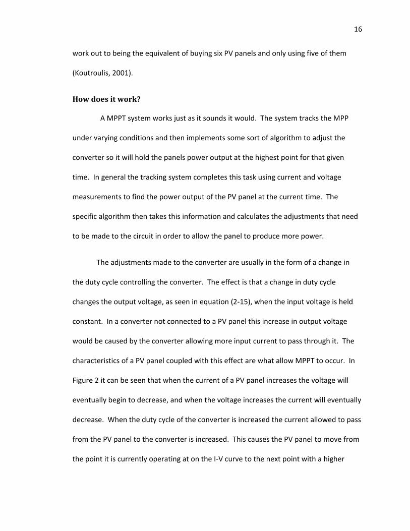
Inductor Current Sensing Technology
The last current sensing technology uses the voltage drop across the second
inductor (L2 in Figure 1). The technology then takes this value with the value of the
current duty cycle to estimate the input current of the converter through the use of a
three-layer feedforward artificial neural network (Yu, 2002) as seen in Figure 9. The
system computes the input current through the use of a feedforward artificial neural
network. The neural network is laid out as in Figure 10, which uses the sigmoidal
function as the activation functions in the hidden layer. The sigmoidal function is
defined as

27
=
(4-7)
The neural network is trained using a backpropagation training algorithm (Yu,
2002) with the inductor voltage drop, duty cycle and input current data from a test
system. Once the neural network is trained it can be implemented in the
microcontroller with fixed weight matrices to estimate the current on the fly. The
power output of the PV panel can be calculated using the estimated current and
measured voltage. These values are then used in the MPPT algorithm already in place
with the resistor current sensing system.
Figure 9. Block diagram of the proposed inductor current sensing control system.
28
Figure 10. Layout of the artificial neural network for inductor current estimation.
This technology improves over the existing technology by not requiring the
sensing resistor, which as stated above automatically adds a power loss to the system.
While there is a power loss associated with the inductor it is already included within the
system and therefore should not be considered an additional loss. This technology also
improves on the current-sensorless system presented above by not needing any
additional regulated voltage supplies. The Op Amps in Figure 8 all require both a
positive and negative supply voltage. This has to be created within the system and will

29
cause additional losses. While these losses may be less than those with the standard
technology removing them will lead to an increase in overall efficiency. All that is
needed with the proposed system is a low pass filter consisting of a simple capacitor and
resistor (Ziegler, 2009), both of which are cheap and readily available.

30
Chapter 5: Simulation Results
Simulation studies are carried out in MATLAB Simulink to validate the converter
and MPPT control for a PV system as is presented in Appendix 2.
Validation of the PV Panel Model
The PV panel model is firstly tested to make sure it is accurate. The results from
the first test can be seen in Figure 11. In this test the I-V curves are found after different
levels of solar irradiance were applied to the model. It can be seen here that while the
voltage remains nearly the same, the current changes greatly with varying irradiance.
Figure 11. I-V curves at different levels of solar irradiance generated by the PV panel model.
0 5 10 15 20 25 30 35 40 450
1
2
3
4
5
6
Voltage (V)
Curr
ent
(A)
I-V curve at different levels of Solar Irradiance (Ir)
Ir = 1kW/m2
Ir = 0.9kW/m2
Ir = 0.8kW/m2
Ir = 0.7kW/m2
Ir = 0.6kW/m2
Ir = 0.5kW/m2

31
In the second test, simulations are performed for the PV panel model with
different cell temperatures. The results are shown in Figure 12. These results from the
model provide a great visual depiction of how small an effect a temperature change has
when compared to a change in irradiance, shown in Figure 11.
Figure 12. I-V curves at different levels of solar cell temperatures generated by the PV panel model.
The Quasi-Double-Boost DC/DC Converter
The DC/DC converter is the next part of the system that needs to be tested. The
converter tests are preformed with a constant voltage source of 36 volts. This is both
for ease of testing and for the accuracy of the results. Other system parameters are set
0 5 10 15 20 25 30 35 40 45 500
1
2
3
4
5
6
Voltage (V)
Curr
ent
(A)
I-V curve at different Solar Cell Temperatures
T = 0C
T = 25C
T = 50C
T = 75C

32
as follows: the switching period of the converter is 50 μs (20 kHz); the inductors are 560
μH and the load resistance R is 330 Ω.
The first aspect of the converter is its characteristics in different operating
modes: CCM and DCM. This can be tested by looking at the inductor currents around
the critical duty cycle found in equation (2-12). With the parameters set above and
equation (2-12) it can be calculated that the critical duty cycle is 0.568. Figure 13 shows
a converter duty cycle on each side of the critical value. From Figure 13 it is shown that
when the duty cycle is 0.60, which is higher than the critical value the converter
operates in CCM. The figure also shows that when the duty cycle is lower than the
critical value at 0.50, the converter operates in DCM. At a duty cycle of 0.55 which is
close to the critical value but still below it the converter is only ever so slightly acting in
DCM.

33
Figure 13. The inductor current of the converter in DCM and CCM.
The next property of the converter to look at is the voltage regulation. To test
voltage regulation the converter is ran at specific duty ratios while input and output
voltages are measured. The regulation ratio is then compared to the ratio calculated by
equation (2-15) in Figure 14. As is shown in the graph, the simulated results for the
voltage regulation are close to what had been calculated. The one main difference is
when the duty cycle is at 95%. At this point the simulated value is a gain of 32.4 while
the calculated value is a gain of 39. This is believed to be due to the simulation being
more accurate to real life where the higher voltage causes more losses though the
components in the converter.
(S)
(S)
(S)
(A)
(A)
(A)

34
Figure 14. Comparison of the calculated and simulated results of voltage regulation for the DC/DC
converter.
The MPPT Control
The P&O MPPT method is implemented in Simulink and added to the converter
circuit and PV panel model. The overall layout of this system is shown in Appendix 2.
The MPPT control unit takes as its input voltage and current measurements from the PV
panel simulation. The control unit then computes the power and sends the information
along with the PV panel voltage value into the P&O algorithm. The algorithm then
decides whether the duty cycle output to the circuit should be increased, decreased or
0 0.1 0.2 0.3 0.4 0.5 0.6 0.7 0.8 0.9 10
5
10
15
20
25
30
35
40
Duty Cycle
Voltage R
egula
tion
Voltage Regulation vs Duty Cycle
Calculated
Simulated

35
kept the same. This new duty cycle is then output to the converter. The process is able
to hold the PV panel at its maximum power output under changing conditions.
In order to test the MPPT control algorithm the entire PV system has to be
simulated. The best way to test the MPPT algorithm is by simulating the PV panel under
various light conditions all while running the converter. This allows the tracking system
to sense the changes in the panel output and correct for them using the duty cycle of
the converter. Figure 15 shows the results of a 40 second simulation of the entire PV
system. It can be seen that the irradiance was first increased from 0 to 1 kW/m2 and
then decreased back down to 0 in a stair step fashion. In the second part of Figure 15
the algorithms reaction to the irradiance is shown in the form of the duty cycle it
outputs. The third graph on Figure 15 shows the resulting solar power output from the
panel.

36
Figure 15. Simulation results of the MPPT control algorithm.
There are a few interesting outcomes worth noting from the results shown in
Figure 15. The first thing that is noticed is the rapid increase in the duty cycle at the
beginning of the simulation. This is something that will only be seen in a simulation and
is a result of the PV panel model being so accurate to real life. When a PV panel is not

37
given any light at all it can actually work in a reverse. This is best described while talking
about a panel hooked up to a battery directly. The reverse leakage current through the
diodes within a solar cell can actually take power away from the battery and emit it
through the PV panel when no light is present. The same is true for this simulation
where the capacitor starts with a slight charge on it. The algorithm is actually doing
exactly what it is supposed to, just backwards. When there is 0 kW/m2 irradiance the PV
panel model is actually taking power out of the capacitor and it is flowing backwards
through the circuit. Even though the amount of power is very small (~-3e-30
) the
algorithm senses it and tries to compensate for it. This compensation is seen in Figure
15 by the duty cycle rapidly increasing at both the beginning and end of the simulation.
Here the algorithm is actually trying to completely shut off the switches within the
converter in order to lessen the loss of power. Since the control algorithm only allows
the converter to operate at a duty cycle from 5% to 95% when the duty cycle shown in
Figure 15 increases to 95% it is reset at 72.5%. Shortly after this reset the irradiance
increases to 0.1 kW/m2, which causes all backward power flow to cease. This allows the
algorithm to settle at the duty cycle which allows the most power flow from the panel to
the converter.
There are two main reasons that the backward power flow seen in Figure 15 is
only a simulation result. In the real system the controller will be powered from the PV
panel in order to minimize losses when it is not needed. This means that when there is
zero irradiance the controller will not be running and, therefore, the converter will
already be in its off state, not allowing reverse power flow. The second reason this

38
should not be seen in the real system is that there is almost never a time when there is
absolutely no irradiance. At night the sun reflects off the moon, there are manmade
lights everywhere and even the stars give off some irradiance that will be seen on the
panel. While this isn’t enough to see a usable amount of power, it is usually enough to
stop the panel from allowing power to flow in reverse.
The next thing to take notice of in Figure 15 is how good the system actually is at
tracking the power output of the PV panel. At very low irradiance values the algorithm
has a slight lag before it settles at the correct value since the duty cycle has to change so
much. This can be seen both when the irradiance is increasing and when it is decreasing
at values of 0.1 and 0.2 kW/m2. This is only seen at these low values and is almost
completely eliminated at higher irradiance values. At the higher values of irradiance the
algorithm is very quick at tracking to the new irradiance value once a change has
occurred. With the simulation only being 40 seconds in total length and having
irradiance changes in steps over the full range of values, the algorithm preformed even
better than expected. This shows that the algorithm should have no problem adjusting
for a quickly changing MPP on partly cloudy days. The next step is to simulate the other
current-sensorless technologies.
Current-Sensorless MPPT Control
Simulation studies are carried out in MATLAB Simulink to validate the proposed
current-sensorless MPPT quasi-double-boost converter for the PV system. These
simulations are completed by using real solar radiation data obtained from National

39
Renewable Energy Laboratory (NREL) to validate the proposed system and control
algorithm. The data was collected from the South Table Mountain site in Golden,
Colorado, on May 31, 2010. During the simulation, the output power of the PV panel is
estimated by the proposed current-sensorless MPPT algorithm and is compared with
the measured output power by using both voltage and current transducers, as shown in
the Figure 16.
Figure 16. The power estimation results.
The proposed current-sensorless algorithm estimates the real output power with
good precision; the estimation errors are less than 1 W during most of the day. Without
knowing the solar radiation, the proposed MPPT algorithm controls the PV system to
track the MPP of the PV panel by using the estimated current and measured voltage.

40
Figure 17 shows the operating points, i.e., the real MPPs, of the panel at various solar
radiation conditions during the day, which are close to ideal MPPs.
Figure 17. The MPPT results of the PV system.
Inductor Current Sensing Technology
Simulation studies are also carried out to validate the inductor current sensing
technology and the resulting MPPT control algorithm. These simulations were
preformed within MATLAB’s Simulink using the neural network laid out as in Figure 10.
The code for the neural network design can be seen in Appendix 2. In order to gather
data to train the system, the converter simulation presented above was run again. The
simulation used a varying duty cycle incremented in small steps and the resulting
inductor voltage drop along with the input voltage and current were recorded. These

41
results were then used to train the artificial neural network. The resulting mean square
error (MSE) output from training can be seen in Figure 18, where the MSE is calculated
by
=
(5-1)
where E is the error between the actual input current and the input current estimated
by the artificial neural network.
Figure 18. Mean square error output during the neural network training.
0 0.5 1 1.5 2 2.5 3
x 104
10-12
10-10
10-8
10-6
10-4
10-2
100
102
Training Step
MS
E
Mean Square Error vs Training Steps
MSE

42
Figure 18 shows that the mean square error stays below 10-1.5
for all inputs by
the end of the training period. To obtain a better understanding of what this actually
means the weights found in testing, the neural network is applied to the data set
recorded through the converter simulation and the estimated input current is compared
against the actual recorded input current. The results of this comparison are shown in
Figure 19.

43
43
Figure 19. Comparison of actual and estimated input current.

44
Figure 19 shows the I-V curve output for both the estimated and the actual PV
panel current. It can be seen that the two curves are very similar. While the two curves
do not exactly match they are close enough to run the MPPT system. The important
aspect of the curve for the MPPT algorithm is not the exact current value, but that the
current is linear in the movement throughout the curve. The algorithm only cares
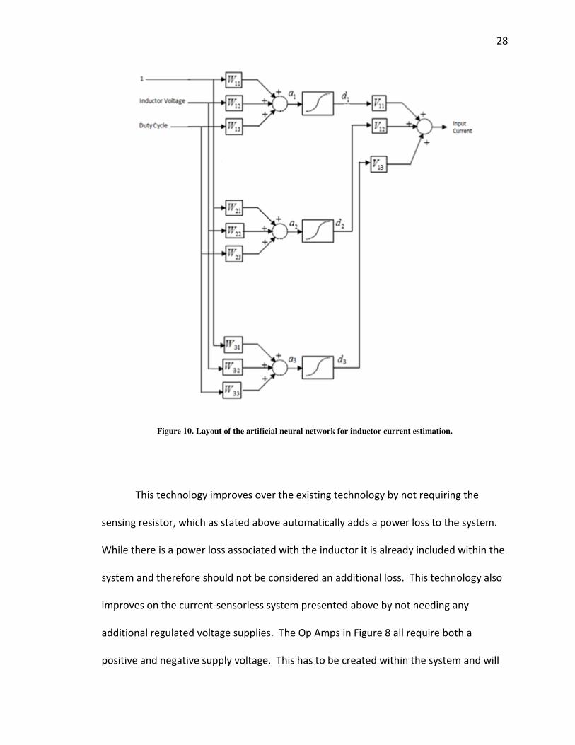
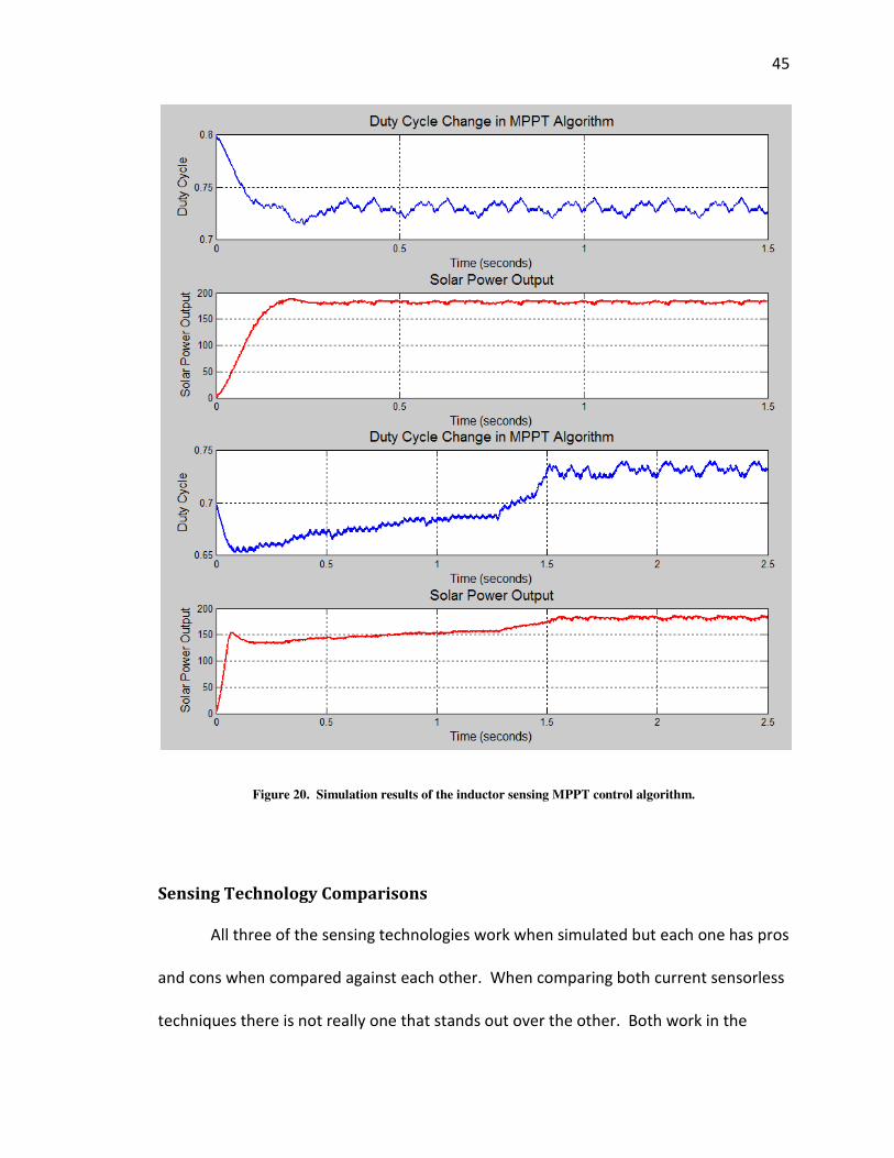
whether the current is increasing or decreasing. This can further be seen by simulating
the MPPT system while using the artificial neural network to estimate the input current
within the algorithm. Figure 20 shows the results of running the system with the
estimated current as an input to the MPPT algorithm. The irradiance is set to 1 kW/m2
and the duty cycle is began to different values, one higher (80%) than the value
expected for the maximum power output and one lower (70%). The algorithm finds the
MPP in both directions to be 184 W, at a duty cycle of 74% which are the same as the
results seen in Figure 15. When comparing the results after the algorithm has reached
the MPP in Figure 20 and in Figure 15, it is again seen that they are the same. This
shows that the algorithm with the inductor current sensing technology is working as
good as the algorithm with the standard sensing technology, though it may be slightly
slower. The inductor current sensing algorithm still manages to find both new MPP
within 1.6 seconds. This is quick enough for the system to work under any normal
working conditions. The next step was to apply the results observed in the simulations
to the actual system.
45
Figure 20. Simulation results of the inductor sensing MPPT control algorithm.
Sensing Technology Comparisons
All three of the sensing technologies work when simulated but each one has pros
and cons when compared against each other. When comparing both current sensorless
techniques there is not really one that stands out over the other. Both work in the

46
lower power application presented here but do not improve on the traditional resistor
sense technology. Where the biggest improvement would be seen is in high power,
high current applications. This is where the resistor sense technology would incur the
most losses. However at these higher powers and currents the current sensorless and
inductor current sense designs would not have any extra losses when compared to a low
power system. Being used in a higher power system may even improve the accuracy of
both systems. The higher current in the current sensorless design would give the
system a more defined voltage ripple to perform calculations off of, improving overall
results. The inductor current sense system would also have a higher inductor voltage
drop to read into the neural network which would allow the system to obtain better
accuracy in the current estimation. This would be due to there being a higher inductor
voltage change correlated to the higher current. The higher current would however
require retraining of the neural network to ensure proper operation.
In low power applications with low current the standard resistor sense
technology is recommended, both for ease of use, cost effectiveness, and reliability. In
applications where the power level may change overtime, such as modular systems
where panels may be added and removed the traditional system is also recommended.
This is because both current sensorless technologies would have to be modified each
time the input power level changed. With the traditional sense technology as long as
the voltage drop across the resistance does not exceed the input rating of the voltage
transducer used to measure it the system will continue to work without any
modification at any power level. In higher power applications that would cause large

47
power losses across a resistive element it is recommended that both the current
sensorless and the inductor current sense technology be evaluated for performance
with the overall system. High power applications are where these systems will excel
over the traditional current sense technology.

48
Chapter 6: Experimental Results
A quasi-double boost DC/DC converter is built and tested with a 175 W
maximum output power PV panel to validate the proposed design and simulation. The
system consists of the PV panel, the DC/DC converter, and an Arduino microcontroller in
which the MPPT algorithm is implemented. A computer with a National Instruments
LabVIEW data acquisition system is used to record data from the system. A picture of
the system can be seen in Figure 21. The code for the MPPT algorithm that is used in
the Arduino can be seen in Appendix 3, and the LabVIEW code for the data acquisition
system can be seen in Appendix 4.
Figure 21. The experimental system.

49
The Quasi-Double-Boost DC/DC Converter
The first aspect of the converter to be verified is the modes of operation; where
the converter switches from CCM to DCM. As shown in Chapter 5 the critical duty cycle
is calculated to be 56.8%. Above 56.8% the converter is expected to run in CCM while
below it should run in DCM. Figure 22, Figure 23 and Figure 24 show the actual results
from the converter being ran at these specific duty cycles. The results are obtained with
the same circuit parameters as in Chapter 5 and the converter input being connected to
the BP PV panel.
Figure 22. Observations from the converter being ran at a 50% duty cycle.
50
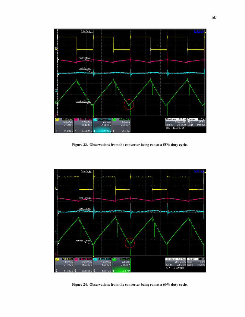
Figure 23. Observations from the converter being ran at a 55% duty cycle.
Figure 24. Observations from the converter being ran at a 60% duty cycle.

51
In Figure 22 it can be seen that when the duty cycle is at 50%, which is below the
critical duty cycle, the circuit is operating in DCM. This can clearly be seen by the
clipping of the lower part of the inductor current wave (circled in red). The results in
Figure 23 are much harder it interpret, as is expected since a duty cycle of 55% is so
close to the critical value of 56.8%. The waveform in Figure 23 does not allow for any
conclusions to be drawn as to whether the converter is in CCM or DCM. Figure 24 can
then be used to ensure that the converter does enter continuous CCM above the critical
duty cycle. The inductor current waveform in Figure 24 shows no signs of current
clipping, thus the converter is clearly operating in CCM.
The next aspect of the converter that needs to be verified is the voltage
regulation. The voltage regulation is found by measuring the input and output voltages
at different duty cycle levels. The output voltage is divided by the input voltage to
obtain the voltage regulation. Figure 25 shows the measured voltage regulation of the
converter compared to the results simulated in Simulink as well as the expected voltage
regulation value that had been calculated from equation (2-15). The experimental
results are measured with the converter connected to the PV panel as an input source
and a 330 Ω resistor bank as an output load.

52
Figure 25. Calculated, simulated, and experimental results of voltage regulation.
As can be seen in Figure 25, the voltage regulation results from the actual
converter are nearly identical to those of the simulated converter up until an 80% duty
cycle. They also closely match the calculated values up until that point. This result
shows two things. First, from the correlation of the regulation ratios 0.05 up to 0.75, it
is observed that the converter is acting as expected. The results are the same as both
the calculated and simulated expectation for the circuit.
Second, something can also be learned from the results above a duty cycle of
75%. The calculations and simulations do not take into account real world parameters
0 0.1 0.2 0.3 0.4 0.5 0.6 0.7 0.8 0.9 10
5
10
15
20
25
30
35
40
Duty Cycle
Voltage R
egula
tion
Voltage Regulation vs Duty Cycle
Calculated
Simulated
Experimental

53
and physical limits on components. The results from Simulink were taken with the
converter connected to an ideal voltage supply at 36 volts. This voltage supply was said
to be able to supply unlimited current while staying at the 36 volt level. The PV panel
however is not an ideal source. This fact is what contributes to the limiting factor on the
voltage regulation of the circuit at the higher duty cycles. As previously presented a PV
panel has a finite limit on the amount of voltage, current, and power it can output.
When the converter is running at higher duty cycle values the PV panel is outputting
very high currents, close to the short circuit value. Since the panel does have a finite
amount of power it can produce this high current causes the panel’s output voltage to
become much lower. This high current, low voltage output characteristic effectively
limits the voltage regulation of the converter by not allowing the circuit the power it
needs to properly boost the output voltage to the expected level. This actual converter
was never expected to reach the calculated voltage regulation value of 39 at a 95% duty
cycle. If this was expected the circuit would have to be completely redesigned to handle
overly high output voltages. To illustrate this, the simulated input and output voltage is
compared to the actual input and output voltage at a 75%-95% duty cycle.
Table 1. Simulated and experimental input and output voltage values of the converter.
Simulation Actual
Duty Cycle Input Voltage (V) Output Voltage (V) Input Voltage (V) Output Voltage (V)
75% 36 252.354 18.4 127
80% 36 319.978 10.6 114
85% 36 439.827 7.11 77.2
90% 36 647.811 4.53 50.9
95% 36 1165.835 2.32 24.4

54
As can be seen in Table 1 at a 95% duty cycle the converter output is dropping 1165.835
volts across the 330 Ω resistor bank. In terms of power this correlates to (P=V2/R) an
output power of 1165.8352 / 330 = 4118.7 W. This clearly shows why the real converter
cannot, and why it is not wanted to, reach even the simulated voltage regulation value
of 32.4 at the 95% duty cycle. The PV panel has a maximum power output of 175 W.
Building a converter that only needs to handle 175 W but at a voltage above 1 kV would
not be economically feasible for most any application.
The last attribute of the converter that needed to be tested was the circuit’s
efficiency. Testing of the efficiency was preformed with the converter being connected
between the output of the PV panel and the 330 Ω resistor bank. The input and output
currents were measured using two Fluke 112 multimeters while the input and output
voltages were measured using a Tektronix TDS 2024 oscilloscope. The test was
performed on the converter alone without any of the current sensing or sensorless
technologies in place. The results of the efficiency test can be seen in Figure 26 and
Table 2. There are a few things to note about Figure 26. First of all is that the efficiency
result for a duty cycle of 95% is not included on the graph. This is simply because the
result is so much lower than the others that it makes the graph harder to see, the result
can still be seen in Table 2. The second thing to notice about the graph is that the
efficiencies are highest when the duty cycle is lowest. This was expected due to the
large inductance values. The final and most compelling aspect of the graph is the almost
uniform efficiency over the band of duty cycles that the MPPT system will use on most

55
normal days. This band covers the duty cycles from 5% to 75%. Over this area there is a
minimum efficiency of 92.4% and a maximum of 98%.
Figure 26. The efficiency of the quasi-double-boost DC/DC converter.
0 0.1 0.2 0.3 0.4 0.5 0.6 0.7 0.8 0.90.82
0.84
0.86
0.88
0.9
0.92
0.94
0.96
0.98
1
Duty Cycle
Eff
icie
ncy
Efficiency vs Duty Cycle
Efficiency

56
Table 2. Results of the converter efficiency test.
Duty
Input
Voltage
(V)
Output
Voltage
(V)
Input
Current
(A)
Output
Current
(A)
Input
Power
(W)
Output
Power
(W) Efficiency
0.05 43 47 0.164 0.147 7.052 6.909 97.9722%
0.1 42.8 53.4 0.217 0.166 9.2876 8.8644 95.4434%
0.15 42.5 62.2 0.3 0.193 12.75 12.0046 94.1537%
0.2 42.5 72.7 0.411 0.227 17.4675 16.5029 94.4777%
0.25 42.3 83 0.541 0.258 22.8843 21.414 93.5751%
0.3 41.6 92.4 0.681 0.286 28.3296 26.4264 93.2819%
0.35 41.1 102 0.844 0.315 34.6884 32.13 92.6246%
0.4 40.7 112 1.021 0.345 41.5547 38.64 92.9859%
0.45 40.6 122 1.22 0.375 49.532 45.75 92.3645%
0.5 39.6 130 1.42 0.400 56.232 52 92.4740%
0.55 38.6 139 1.655 0.428 63.883 59.492 93.1265%
0.6 37.4 145 1.872 0.447 70.0128 64.815 92.5759%
0.65 32.4 147 2.235 0.456 72.414 67.032 92.5677%
0.7 28.2 156 2.841 0.485 80.1162 75.66 94.4378%
0.75 21.6 145 3.224 0.446 69.6384 64.67 92.8654%
0.8 14.1 116 3.325 0.359 46.8825 41.644 88.8263%
0.85 8.6 87.1 3.45 0.285 29.67 24.8235 83.6653%
0.9 8.15 86.7 3.475 0.276 28.32125 23.9292 84.4920%
0.95 2.18 26.2 3.452 0.081 7.52536 2.1222 28.2006%
The MPPT Control
The MPPT system is also tested over a variety of situations. The algorithm is
implemented by connecting one panel to the quasi-double-boost converter. The duty
cycle of this converter is controlled by the Arduino microcontroller that is fed
information by the LabView data acquisition system. A second, duplicate panel is them
connected to a fixed resistance directly. The value of this resistance is set so that the
panel will be able to output the maximum power as described in the PV panel manual
(Appendix 1). The resistance is calculated by taking the rated voltage at maximum

57
power (VMP) of the panel (36.1 V) and dividing it by the rated current at maximum
power (IMP) of the panel (4.85 A). This gives a resistance of 7.44 Ω. The resistor
connected to the second panel has a resistance of 6.3 Ω at room temperature.
Resistance rises with increased temperature, and the current through a resistor
produces heat thereby raising the temperature of the resistor. The 6.3 Ω resistor
measures out to 7.36 Ω while under a load current of 4.85 A, making it ideal for use with
this specific PV panel.
The LabView system that sends the information to the microcontroller to run the
MPPT system also records the information about voltage and current output from each
panel. These values for each panel are then multiplied together to obtain the power
output of each panel to compare against one another. The voltage is measured using a
precision resistor divider network to lower the voltage down to an acceptable level to
measure with the data acquisition system. The currents of both panels are measured in
the ground loop (the line connecting the ground of the panel to the ground of the
resistor bank) using the voltage drop across a precision current sensing resistor of 0.1 Ω.
The first MPPT test is preformed on a cloudy overcast day. A day like this is
where the MPPT algorithm should best outperform the fixed resistance. This is because
of two reasons, the first being that the fixed resistance is set to obtain the most power
on a sunny day as recommended by the PV panel manual (Appendix 1). When clouds
are present the fixed resistance cannot compensate for them as the algorithm should be
able to. Secondly the algorithm should be able to adjust slightly to compensate for the

58
differing thickness of each passing cloud in order to obtain the highest power output at
any point in time.
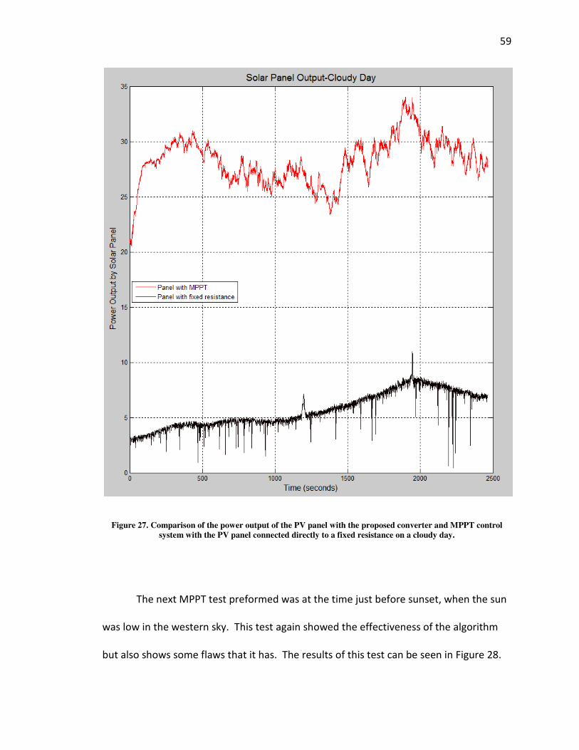
The results from this test can be seen in Figure 27. The PV panel connected to
the MPPT system clearly has the advantage over the system with the fixed resistance.
The fixed resistance panel’s output is dependent on how much sunlight is getting
through the clouds and only that. The fixed resistance cannot change the power point
the panel is currently operating at to ensure maximum power output. The converter
can be adjusted by the algorithm to compensate for the clouds. This can clearly be seen
in the first seconds of the power output of the panel with the MPPT system. Here the
power is initially lower at 20.5 W when the controller is first turned on, however the
algorithm quickly searched out the MPP and allows the panel to operate there (about 30
W). Over the same timeframe the panel with the fixed resistances output increased
from 3.5 to 4.75 W. Figure 27 also shows that the MPPT algorithm does work even
under rapidly changing conditions. As the irradiance increases on the panel with the
fixed resistance, causing more power output the algorithm also follows this increase in
irradiance. The algorithm then also follows the decrease of irradiance towards the end
of the data in Figure 27.
59
Figure 27. Comparison of the power output of the PV panel with the proposed converter and MPPT control
system with the PV panel connected directly to a fixed resistance on a cloudy day.
The next MPPT test preformed was at the time just before sunset, when the sun
was low in the western sky. This test again showed the effectiveness of the algorithm
but also shows some flaws that it has. The results of this test can be seen in Figure 28.

60
In the very first few seconds of Figure 28 the algorithm can be seen turning on and
quickly finding the MPP of the PV panel. From that point on, the power steadily
decreases as the sun goes down. As this is happening the power output by the panel
connected to the converter and controlled by the algorithm never drops below the
power output by the panel with a fixed resistance.
What is most noticeable about Figure 28 is at about 550 seconds in when the
power output by the MPPT panel falls from 2.5 W to about 0.25 W. This is because at
this low of light condition the algorithm is running the converter at the very extremes of
its duty cycle range, in this case very close to 0.05. This drop in power happens when
the converter is operating at a duty cycle of 5% and tries to climb even lower. As
protection for the converter the algorithm is never allowed to set the duty cycle greater
than 95% or lower than 5%. When the duty cycle tries to exceed one of these values it
is reset to a value of 50%. After the reset occurs the algorithm again searches out the
MPP of the PV panel. Once the system finds the MPP it is able to hold there for a little
while before being reset again. The system finds the MPP and then resets once more
before the sun goes down too far to give off any measurable power. This reset
condition could be corrected by letting the algorithm hold the duty cycle at 5% but not
allow it to go any lower thereby allowing the system to work without a reset. However
this would also allow for more chance of the circuit being damaged by certain
unforeseen conditions. If wires from two separate panels come into contact and short
out it would be much better for the circuit if it was forced to reset to a 50% duty cycle
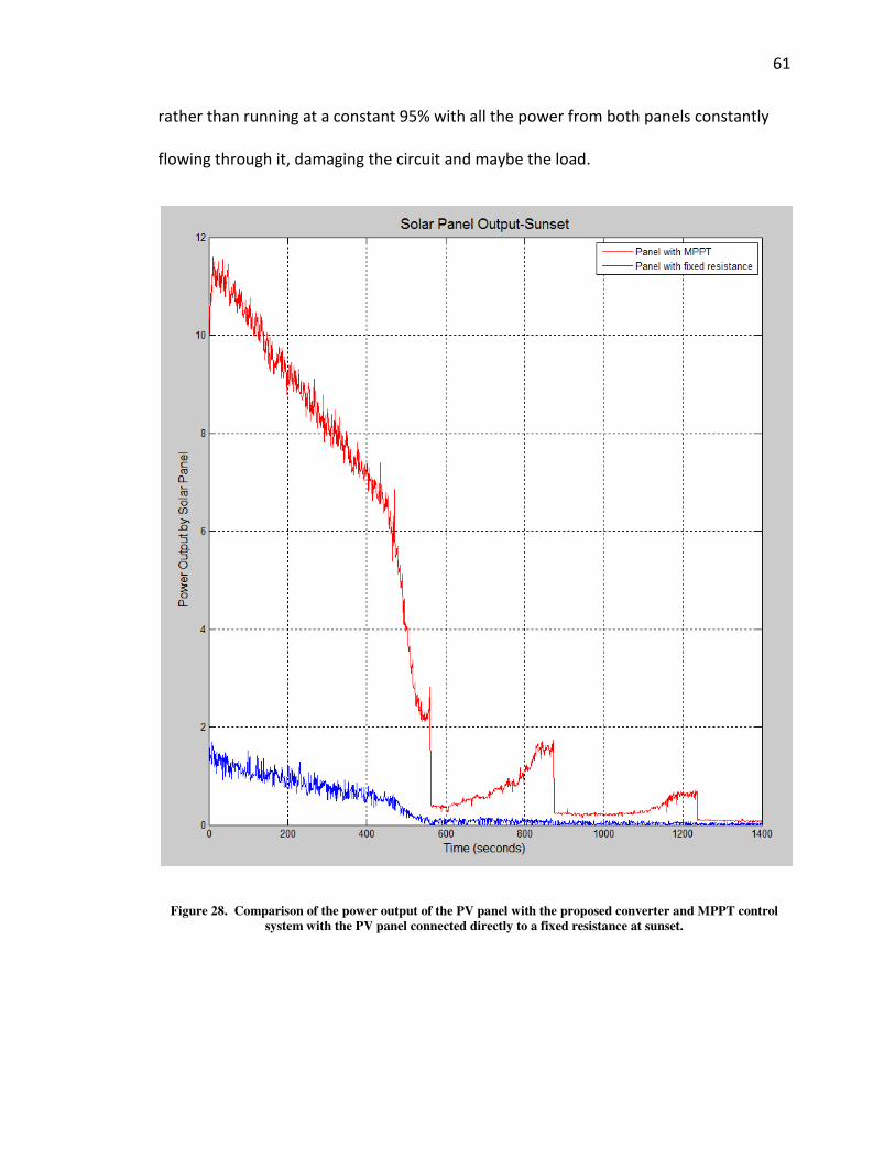
61
rather than running at a constant 95% with all the power from both panels constantly
flowing through it, damaging the circuit and maybe the load.
Figure 28. Comparison of the power output of the PV panel with the proposed converter and MPPT control
system with the PV panel connected directly to a fixed resistance at sunset.

62
The final MPPT test can be seen in Figure 29. In this figure the system is ran for
almost a full day when there was almost no clouds in the sky. A system reset as
described above can again be seen in the very beginning of this graph. The figure also
shows the same results seen in the figures above where there is a great improvement
when using the system compared to using a fixed resistance. A notable aspect of this
figure is how much of an improvement there is when the system is at maximum power
output when the sun is at its highest point in the sky. This large improvement is due to
the test being performed during a winter month. In the winter months the sun is at a
lower angle in the sky so it is not hitting the PV panel dead on. This causes less light to
be absorbed within the panel than would be during a summer month. The lower light
absorption due to the angle can also be seen in that the maximum power output barely
exceeds 100 watts when both panels are rated at 175 watts. During a summer month
when the sun is hitting the panel directly and the PV panel is outputting the maximum
rated power these two curves should be identical at the peak point. This is because the
fixed resistance is implemented according to the values of voltage and current at
maximum power. While the MPPT circuit could perform better during all other times of
the day, it would have the same performance as the fixed resistance over the time when
the panel is operating at its rated power output. The values of voltage and current at
maximum power are finite and cannot be exceeded by the tracking circuit.

63
Figure 29. MPPT Comparison of the power output of the PV panel with the proposed converter and MPPT
control system with the PV panel connected directly to a fixed resistance over a full sunny day.

64
Current-Sensorless MPPT Control
The next experiment is to test the effectiveness of the proposed current-
sensorless MPPT system. It utilizes the voltage ripple of the input capacitor to calculate
the input current of the converter through equations (4-5) and (4-6). Figure 30 shows
the current estimation result, where the estimated value closely follows the actual
current value. The maximum estimation error is less than 0.2 A, which indicates that the
maximum error of the power estimation is less than 8 W for the converter.
Figure 30. The current estimation results.
Using the estimated current, the MPPT tracking performance in a high radiation
condition is shown in Figure 31. The initial duty ratio is set low so that the tracking
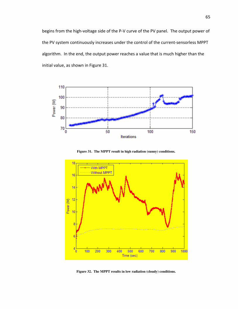
65
begins from the high-voltage side of the P-V curve of the PV panel. The output power of
the PV system continuously increases under the control of the current-sensorless MPPT
algorithm. In the end, the output power reaches a value that is much higher than the
initial value, as shown in Figure 31.
Figure 31. The MPPT result in high radiation (sunny) conditions.
Figure 32. The MPPT results in low radiation (cloudy) conditions.

66
Figure 32 compares the power output of the PV panel connected to a fixed load
of 330 Ω through the quasi-double-boost converter with MPPT control against a second
identical panel connected directly to a fixed load without the converter. This test was
done in low radiation conditions to show the effectiveness of the system for all
operating conditions. Figure 32 shows that the output power of the PV panel with the
tracking system is much more than that without the MPPT, which confirms the
effectiveness of using the current-sensorless MPPT control.

67
Chapter 7: Conclusions, Contributions, and Recommendation for
Future Work
In order to maintain the highest power output from a PV panel at all times a high
efficiency converter coupled with a MPPT system must be used. In this research a high-
efficiency quasi-double-boost DC/DC converter was designed and implemented. A fast
reacting and accurate MPPT algorithm was implemented to control the converter and
make sure the PV panel is always outputting the maximum power available at a given
time. Results are presented showing the output power improvement over a standard
panel with a fixed load. Three separate current sensing and sensorless methods are
presented to ensure the entire system operates with the highest possible efficiency.
In future work it is recommended that all three current sensing technologies be
implemented with identical converters and PV panels, so they can truly be tested
against one another. If the experiment could be ran for an extended period of time with
the converter, microcontroller and all voltage regulators needed for the microcontroller
and the current sensing technologies being powered off the PV panel then the overall
efficiency of each system could be realized.
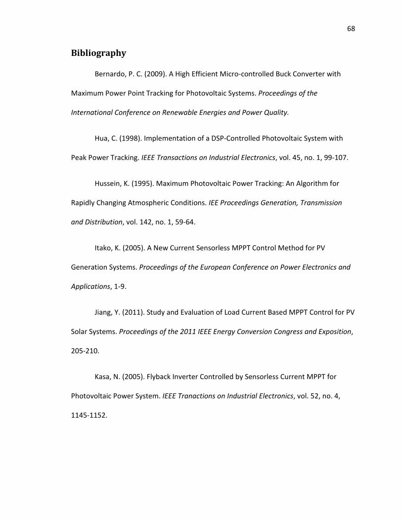
68
Bibliography
Bernardo, P. C. (2009). A High Efficient Micro-controlled Buck Converter with
Maximum Power Point Tracking for Photovoltaic Systems. Proceedings of the
International Conference on Renewable Energies and Power Quality.
Hua, C. (1998). Implementation of a DSP-Controlled Photovoltaic System with
Peak Power Tracking. IEEE Transactions on Industrial Electronics, vol. 45, no. 1, 99-107.
Hussein, K. (1995). Maximum Photovoltaic Power Tracking: An Algorithm for
Rapidly Changing Atmospheric Conditions. IEE Proceedings Generation, Transmission
and Distribution, vol. 142, no. 1, 59-64.
Itako, K. (2005). A New Current Sensorless MPPT Control Method for PV
Generation Systems. Proceedings of the European Conference on Power Electronics and
Applications, 1-9.
Jiang, Y. (2011). Study and Evaluation of Load Current Based MPPT Control for PV
Solar Systems. Proceedings of the 2011 IEEE Energy Conversion Congress and Exposition,
205-210.
Kasa, N. (2005). Flyback Inverter Controlled by Sensorless Current MPPT for
Photovoltaic Power System. IEEE Tranactions on Industrial Electronics, vol. 52, no. 4,
1145-1152.

69
Koutroulis, E. (2001). Development of a Microcontroller-Based, Photovoltaic
Maximum Power Point Tracking Control System. IEEE Transactions on Power Electronics,
vol. 16, no. 1, 46-54.
Lohmeier, C. (2011). A Current-Sensorless MPPT Quasi-Double-Boost Converter
for PV Systems. Proceedings of the 2011IEEE Energy Conversion Congress and Exposition,
1069-1075.
Morales-Saldaña, J. A. (2006). Modeling and Control of a Cascaded Boost
Converter with a Single Switch. IECON 2006 - 32nd Annual Conference on IEEE Industrial
Electronics, 591-596.
Mrabti, T. (2009). Regulation of Electric Power of Photovoltaic Generators With
DC-DC Converter (Buck Type) andMPPT Command. ICMCS '09. International Conference
on Multimedia Computing and Systems, 322-326.
Nabulsi, A. A. (2009). A 300 Watt Cascaded Boost Converter Design for Solar
Energy Systems. EPECS '09. International Conference on Electric Power and Energy
Conversion Systems, 1-4.
Orellana, M. (2010). Four Switch Buck-Boost Converter for Photovoltaic DC-DC
Power Applications. IECON 2010 - 36th Annual Conference on IEEE Industrial Electronics
Society, 469-474.

70
Pan, C. (1999). A Fast Maximum Power Point Tracker for Photovoltaic Power
Systems. Proceedings of the 25th Annual Conference of the IEEE Industrial Electronics
Society Conference, 390-393.
Rensburg, J. v. (2008). Double-Boost DC to DC Converter. Proceedings of the 34th
Annual Conference of the IEEE Industrial Electronics Society Conference, 701-711.
Salas, V. (2006). Review of the Maximum Power Point Tracking Algorithms for
Stand-Alone Photovoltaic Systems. Solar Energy Materials & Solar Cells, vol. 90, no. 11,
1555-1578.
Shanthi, T. (2007). Power Electronic Interface for Grid-Connected PV array using
Boost Converter and Line-Commutated Inverter with MPPT. Proceedings of the IEEE
International Conference on Intelligent and Advanced Systems, 882-886.
Tsai, H. L. (2008). Development of Generalized Photovoltaic Model Using
MATLAB/SIMULINK. Proceedings of the World Congress on Engineering and Computer
Science. San Francisco, USA.
Wenham, S. R. (2009). Applied Photovoltaics. Earthscan.
Yu, X. (2002). A General Backpropagation Algorithm for Feedforward Neural
Networks Learning. IEEE Transactions on Neural Networks, 251-254.
Ziegler, S. (2009). Lossless Inductor Current Sensing Method With Improved
Frequency Response. IEEE Transactions on Power Electronics, vol. 24, no. 5, 1218-1222.

71
Appendix 1 - BP Solar Panel Model SX 3175

72
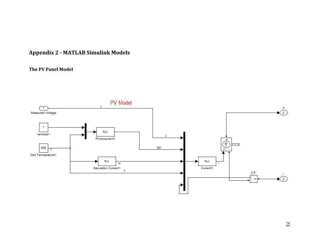
73
73
Appendix 2 - MATLAB Simulink Models
The PV Panel Model
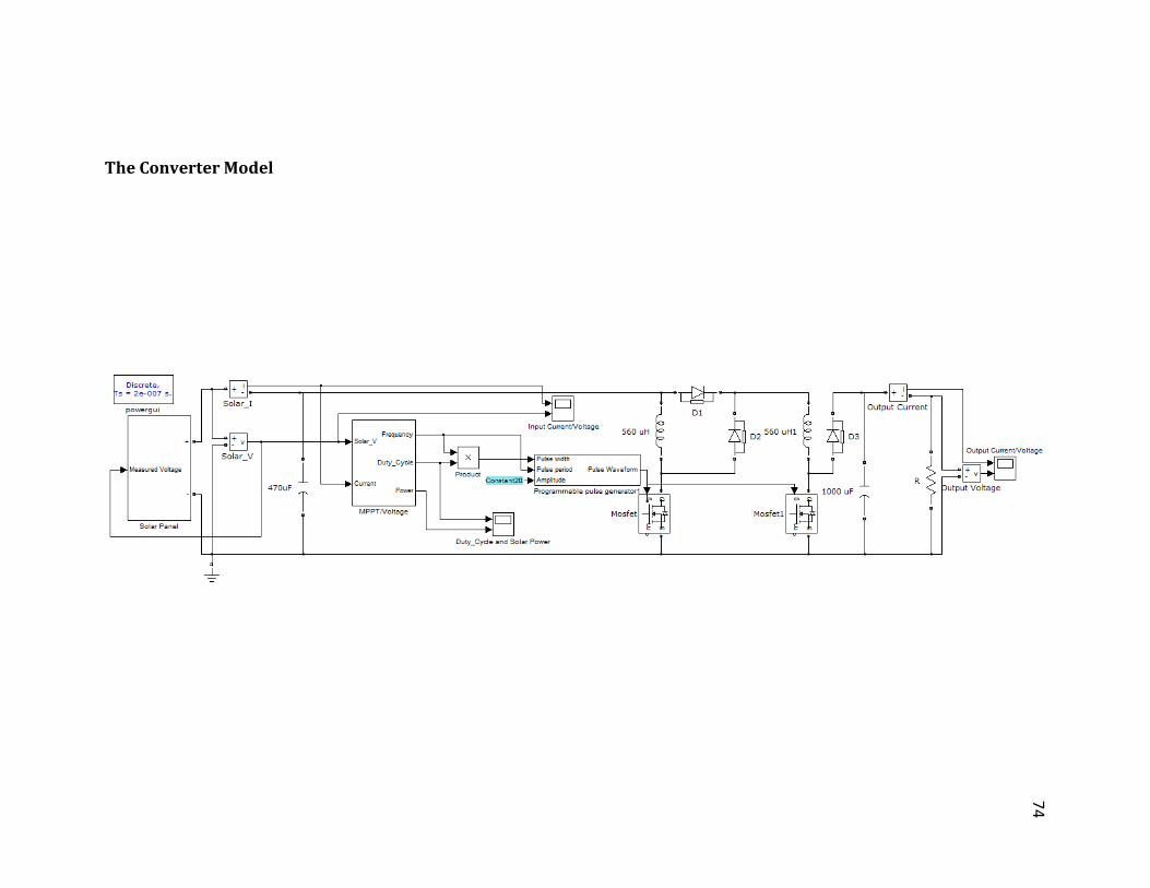
74
74
The Converter Model
75
The MPPT Control Block

76
The MPPT Code
function [Voltage,Power_P,Power,Freq,Test,Duty,Count]=
fcn(Power_Prev,... SV_Prev,Solar_V,Current,O_Freq,Change,Duty_I,T)
Power = Solar_V * Current; Duty = Duty_I; Freq = O_Freq; Count = T + 1; rate = 0.001; Power_P = Power_Prev; Voltage = SV_Prev; if Count == 1e4 %*************************MPPT********************** if abs(1-Power/Power_Prev) <= rate else if (Duty > 0.1 && Duty < 0.95) if Power>Power_Prev if Solar_V>SV_Prev Duty = Duty - Change; else Duty = Duty + Change; end else if Solar_V>SV_Prev Duty = Duty + Change; else Duty = Duty - Change; end end else Duty = .7; end Power_P = Power; Voltage = Solar_V; end Count = 0; %***********************END MPPT********************** end end

77
Code for Artificial Neural Network
clear; clc; Volt = xlsread('New_Data.xlsx', 'Q:Q'); Current = xlsread('New_Data.xlsx', 'O:O'); Duty = xlsread('New_Data.xlsx', 'R:R'); Vin = xlsread('New_Data.xlsx', 'P:P'); Num_Nu = 3; Num_Inp = 3; Gg = 0.42; Gm = 0.3; Dv = zeros(1,Num_Nu); Dv_prev = zeros(Num_Nu,1); Dw = zeros(Num_Nu,Num_Inp); Dw_prev = zeros(Num_Nu,Num_Inp); i_wgt = [0.0292;0.6006;0.7162;]; runs = 27264;
for (i = 1:Num_Nu) for (j = 1:Num_Inp) w(i,j) = rand(); end end for (i = 1:Num_Nu) v(i,1) = i_wgt(i,1); end for (ep = 1:runs) E = 0; yh = 0; Z = Volt(ep); D = Duty(ep); G = Vin(ep); C = Current(ep); % T = rand(); x = [1;Z;D]; a = w*x; d = 1.0 ./ (1.0 + exp(-a)); for (i = 1:Num_Nu) yh = yh + d(i)*v(i); end y = Current(ep); ey = y - yh; ea = (v.*ey) .* (d.*(1-d)); E = .5*abs(ey).*abs(ey); MSE(ep) = E; EP(ep) = (ep); Dv = (Gg*ey).*d + Gm.*Dv_prev; Dv_prev = Dv; Dw = (Gg*ea)*x' + Gm.*Dw_prev; Dw_prev = Dw; v = v + Dv; w = w + Dw; end semilogy(EP,MSE,'r','LineWidth',2) xlabel 'Training Step'

78
ylabel 'MSE' title 'Mean Square Error vs Training Steps' legend('MSE') grid on figure;

79
Code to Test the Results of Training the Artificial Neural Network
EP = 0;MSE = 0;ZT = 0;ep = 0;YA = 0;YH = 0; Num_of_Test = 13632; for (ep = 1:Num_of_Test) E = 0; yh = 0; Z = Volt(ep); D = Duty(ep); x = [1;Z;D]; a = w*x; d = 1.0 ./ (1.0 + exp(-a)); for (i = 1:Num_Nu) yh = yh + d(i)*v(i); end y = Current(ep); ey = y - yh; ea = (v.*ey) .* (d.*(1-d)); E = .5*abs(ey).*abs(ey); MSE(ep) = E; EP(ep) = (ep); YA(ep) = y; YH(ep) = yh; ZT(ep) = G; end figure; subplot(2,1,1) semilogy(ZT,MSE,'gx','LineWidth',2) xlabel 'Solar Voltage (V)' ylabel 'MSE' title 'Solar Voltage vs Mean Square Error' legend('MSE') grid on
subplot(2,1,2) plot(ZT,YA,'ro','LineWidth',2) hold on; plot(ZT,YH,'bx','LineWidth',2) xlabel 'Solar Voltage (V)' ylabel 'Actual/Estimated Current (A)' title 'I-V Curve' legend('Actual Current', 'Estimated Current') grid on

80
Appendix 3 - MPPT Code Implemented in the Arduino
int maxDuty = 800; long csPin = A0; long vsPin = A2; int numberAnalogReads; int duty; long prevPower; long prevVoltage;
void setup() Serial.begin(9600); TCCR1A = 242; TCCR1B = 25; ICR1 = maxDuty; OCR1A = 400; OCR1B = maxDuty; DDRB = _BV(PB1) | _BV(PB2); pinMode (csPin, INPUT); pinMode (vsPin, INPUT); int numberAnalogReads = 2; int duty = 400; long prevPower = 0; long prevVoltage = 0;
void loop() duty = OCR1A; long current = readAndAvgC(); long voltage = readAndAvgV(); long power = current * voltage; if (abs(power - prevPower) > 500) algorithm (voltage, power); delayMore ();
// Subroutines
long readAndAvgC () long reading = 0; long temp = 0; for (int x = 0; x <= 0; x++) delay(400); temp = analogRead(csPin); delay(50); temp = temp + analogRead(csPin); delay(50); temp = temp + analogRead(csPin);

81
delay(50); temp = temp + analogRead(csPin); delay(50); temp = temp + analogRead(csPin); delay(50); temp = temp + analogRead(csPin); delay(50); reading = temp / 6; return reading;
long readAndAvgV () long reading = 0; long temp = 0; for (int x = 0; x <= 0; x++) delay(0); temp = analogRead(vsPin); delay(50); temp = temp + analogRead(vsPin); delay(50); temp = temp + analogRead(vsPin); delay(50); temp = temp + analogRead(vsPin); delay(50); temp = temp + analogRead(vsPin); delay(50); temp = temp + analogRead(vsPin); delay(50); reading = temp / 6; return reading;
void algorithm (long voltage, long power) if (duty > 40 && duty < 760) if (power>prevPower) if (voltage<(prevVoltage+10))//> OCR1A = OCR1A - 4; else OCR1A = OCR1A + 4; else if (voltage<(prevVoltage+10))//> OCR1A = OCR1A + 4;

82
else OCR1A = OCR1A - 4; else OCR1A = 400; prevPower = power; prevVoltage = voltage; return;
void delayMore () delay(1000); return;

83
Appendix 4 - LabVIEW Data Acquisition System