hermite weno schemes for hamilton–jacobi...

Journal of Computational Physics 204 (2005) 82–99

www.elsevier.com/locate/jcp

Hermite WENO schemes for Hamilton–Jacobi equations

Jianxian Qiu a,1, Chi-Wang Shu b,*,2

a Department of Mechanical Engineering, National University of Singapore, Singapore 119260, Singaporeb Division of Applied Mathematics, Brown University, Providence, RI 02912, USA

Received 23 August 2004; accepted 4 October 2004

Available online 11 November 2004

Abstract

In this paper, a class of weighted essentially non-oscillatory (WENO) schemes based on Hermite polynomials,

termed HWENO (Hermite WENO) schemes, for solving Hamilton–Jacobi equations is presented. The idea of the

reconstruction in the HWENO schemes comes from the original WENO schemes, however both the function and its

first derivative values are evolved in time and used in the reconstruction, while only the function values are evolved

and used in the original WENO schemes. Comparing with the original WENO schemes of Jiang and Peng [Weighted

ENO schemes for Hamilton–Jacobi equations, SIAM Journal on Scientific Computing 21 (2000) 2126] for Hamilton–

Jacobi equations, one major advantage of HWENO schemes is its compactness in the reconstruction. Extensive numer-

ical experiments are performed to illustrate the capability of the method.

� 2004 Elsevier Inc. All rights reserved.

MSC: 65M06; 65M99; 70H20

Keywords: WENO scheme; Hamilton–Jacobi equation; Hermite interpolation; High order accuracy

1. Introduction

In this paper, we construct a class of fifth order WENO schemes based on Hermite polynomials, termed

HWENO schemes, for solving the Hamilton–Jacobi (HJ) equations:

0021-9

doi:10

* C

E-m1 R2 R

and Te

Additi

991/$ - see front matter � 2004 Elsevier Inc. All rights reserved.

.1016/j.jcp.2004.10.003

orresponding author. Tel.: +1 401 863 2549; fax: +1 401 863 1355.

ail addresses: [email protected] (J. Qiu), [email protected] (C.-W. Shu).

esearch partially supported by NUS Research Project R-265-000-118-112 and NNSFC grant 10371118.

esearch partially supported by the Chinese Academy of Sciences while the author was in residence at the University of Science

chnology of China (grant 2004-1-8) and at the Institute of Computational Mathematics and Scientific/Engineering Computing.

onal support is provided by ARO grant W911NF-04-1-0291, NSF grant DMS-0207451 and AFOSR grant F49620-02-1-0113.

mailto:[email protected]

mailto:[email protected]

J. Qiu, C.-W. Shu / Journal of Computational Physics 204 (2005) 82–99 83

/t þ Hðrx/Þ ¼ 0;

/ðx; 0Þ ¼ /0ðxÞ;

�ð1:1Þ

where x = (x1, . . . ,xd) are d-spatial variables. The HJ equations appear often in applications, such as in

control theory, differential games, geometric optics and image processing. The solutions to (1.1) typicallyare continuous but with discontinuous derivatives, even if the initial condition /0(x) 2 C1. It is well

known that the HJ equations are closely related to conservation laws, hence successful numerical meth-

ods for conservation laws can be adapted for solving the HJ equations. Along this line we mention the

early work of Osher and Sethian [20] and Osher and Shu [21] in constructing high order ENO (essentially

non-oscillatory) schemes for solving the HJ equations. These ENO schemes for solving the HJ equations

were based on ENO schemes for solving hyperbolic conservation laws in [9,26,27]. ENO schemes for

solving the HJ equations on unstructured meshes were constructed in [15]. More recently, ENO schemes

based on radial basis functions were constructed in [6]. Central high resolution schemes were developedin [3,4,14]. Finite element methods suitable for arbitrary triangulations were developed in [1,5,10,16].

Finally, most relevant to our work, we mention the WENO schemes for solving the HJ equations [12]

by Jiang and Peng, based on the WENO schemes for solving conservation laws [18,13]. Zhang and

Shu [29] further developed high order WENO schemes on unstructured meshes for solving two dimen-

sional HJ equations.

We now review WENO schemes in more detail as they are most relevant to our work in this paper.

WENO schemes have been designed in recent years as a class of high order finite volume or finite dif-

ference schemes to solve hyperbolic conservation laws and Hamilton–Jacobi equations with the propertyof maintaining both uniform high order accuracy and an essentially non-oscillatory shock transition.

The first WENO scheme is constructed in [18] for a third order finite volume version in one space

dimension. In [13], third and fifth order finite difference WENO schemes in multi space dimensions

are constructed, with a general framework for the design of the smoothness indicators and nonlinear

weights. Finite volume WENO schemes on unstructured and structured meshes are designed in, e.g.

[8,10,17,22]. WENO schemes are designed based on the successful ENO schemes in [9,26,27]. Both

ENO and WENO schemes use the idea of adaptive stencils in the reconstruction procedure based on

the local smoothness of the numerical solution to automatically achieve high order accuracy and anon-oscillatory property near discontinuities. For a detailed review of ENO and WENO schemes, we

refer to the lecture notes [25].

The framework of the finite volume and finite difference WENO schemes is to evolve only one degree

of freedom per cell, namely the cell average for the finite volume version or the point value at the center

of the cell for the finite difference version. In [23,24] we presented a class of WENO schemes based on

Hermite polynomials, termed HWENO schemes, for solving one and two dimensional nonlinear hyper-

bolic conservation law systems. The main difference between the Hermite WENO scheme designed in

[23,24], see also related earlier work in [2,7,19,28], and the traditional WENO schemes is that the formerhas a more compact stencil than the latter for the same order of accuracy. This compactness is achieved

by evolving both the function and its first derivative values in time and they are both used in the recon-

struction in HWENO schemes. As a result, a fifth order one dimensional HWENO reconstruction uses

only three points, while a fifth order one dimensional WENO reconstruction would need to use five

points. Numerical examples in [23,24] demonstrate that HWENO schemes work well for solving hyper-

bolic conservation laws.

In this paper, based on the HWENO methodology for conservation laws in [23,24], we develop HWENO

schemes to solve the HJ equations. We evolve both the solution / at the grid points and the cell averages ofthe x and y derivatives of the solution /. Both the point values of the solution and the cell averages of its

derivatives are used to reconstruct the point values of the derivatives at the grid points and at the interfaces

of the cells. Comparing with the original WENO schemes of Jiang and Peng [12], one major advantage of

84 J. Qiu, C.-W. Shu / Journal of Computational Physics 204 (2005) 82–99

HWENO schemes is its compactness in the reconstruction. For example, in the one dimensional case, six

points are needed in the stencil for a fifth order WENO reconstruction, while only four points are needed

for a fifth order HWENO reconstruction. We do remark that HWENO schemes are more costly in com-

putation and storage than the regular WENO schemes on the same mesh, since both the solution and its

derivatives must be stored and evolved in time. It is however our experience that HWENO schemes aremore accurate than WENO schemes on the same mesh for most problems.

The organization of this paper is as follows. In Section 2, we describe in detail the construction and

implementation of the HWENO schemes with Runge–Kutta time discretizations, for one and two dimen-

sional Hamilton–Jacobi equations (1.1). In Section 3 we provide extensive numerical examples to demon-

strate the behavior of the HWENO schemes. Concluding remarks are given in Section 4.

2. The construction of Hermite WENO schemes for the Hamilton–Jacobi equations

In this section we will present the details of the construction of Hermite WENO schemes for both one

and two dimensional Hamilton–Jacobi equations.

2.1. One dimensional case

We first consider the one dimensional Hamilton–Jacobi equation (1.1). For simplicity, we assume that

the grid points {xi} are uniformly distributed with the cell size xi+1 � xi = Dx and cell centersxiþ1

2¼ 1

2ðxi þ xiþ1Þ. We also denote the cells by I i ¼ ½xi�1

2; xiþ1

2�. This assumption is not essential: the method

can be easily defined for non-uniform meshes.

Let u = /x, and taking the x derivative of (1.1), we obtain the conservation law:

ut þ HðuÞx ¼ 0;

uðx; 0Þ ¼ u0ðxÞ:

�ð2:1Þ

We denote /i(t) = /(xi,t) and the cell averages of u as uiðtÞ ¼ 1Dx

RIiuðx; tÞ dx. Integrating (2.1) over the cell Ii

we obtain an equivalent form:

ddt/iðtÞ ¼ �Hðuðxi; tÞÞ;ddt uiðtÞ ¼ � 1

Dx ðHðuðxiþ1=2; tÞÞ � Hðuðxi�1=2; tÞÞÞ:

(ð2:2Þ

We approximate (2.2) by the following scheme:

d/iðtÞdt ¼ � ~Hi;

duiðtÞdt ¼ � 1

Dx ðH iþ1=2 � H i�1=2Þ;

(ð2:3Þ

where the numerical fluxes ~Hi and H iþ1=2 in (2.3) are subject to the usual conditions for numerical fluxes,

such as monotonicity, Lipschitz continuity and consistency with the physical flux H(u). For choices ofnumerical fluxes suitable for the HJ equations we refer to, e.g. [21]. In this paper we use the simple

Lax–Friedrichs flux defined by:

~Hi ¼ Hu�i þuþi

2

� �� a

2uþi � u�i� �

;

H iþ1=2 ¼ 12

Hðu�iþ1=2Þ þ Hðuþiþ1=2Þ � aðuþiþ1=2 � u�iþ1=2Þ� �

;ð2:4Þ

where u�i and u�iþ1=2 are the numerical approximations to the point values of u(xi,t) and u(xi+1/2,t), respec-

tively, from left and right, and a = maxujH 0(u)j.


The method of lines ODE (2.3), written in the form

wt ¼ LðwÞ

is then discretized in time by a total variation diminishing (TVD) Runge–Kutta method [26], for examplethe third order version given by:

wð1Þ ¼wn þ DtLðwnÞ;wð2Þ ¼3

4wn þ 1

4wð1Þ þ 1

4DtLðwð1ÞÞ; ð2:5Þ

wnþ1 ¼13wn þ 2

3wð2Þ þ 2

3DtLðwð2ÞÞ:

The key component of the HWENO schemes is the reconstruction, from point values {/i} and the cell

averages fuig to the points values fu�i ; u�iþ1=2g. This reconstruction should be both high order accurate and

essentially non-oscillatory. We outline the procedure of this reconstruction for the fifth order accurate case

in the following.Step 1. Reconstruction of fu�i g by HWENO from f/i; uig.

1. Given the small stencils S0 = {xi� 2,xi� 1,xi,Ii� 1}, S1 = {xi� 1,xi,xi+1,Ii+1}, S2 = {xi� 2,xi� 1,xi,xi+1} and

the bigger stencil T ¼ fS0; S1; S2g, we construct Hermite cubic reconstruction polynomials p0(x), p1(x),

p2(x) and a fifth-degree reconstruction polynomial q(x) such that:

p0ðxiþjÞ ¼ /iþj; j ¼ �2;�1; 0;1

Dx

ZI i�1

p00ðxÞ dx ¼ ui�1:

p1ðxiþjÞ ¼ /iþj; j ¼ �1; 0; 1;1

Dx

ZI iþ1

p01ðxÞ dx ¼ uiþ1:

p2ðxiþjÞ ¼ /iþj; j ¼ �2;�1; 0; 1:

qðxiþjÞ ¼ /iþj; j ¼ �2;�1; 0; 1;1

Dx

ZI iþj

q0ðxÞ dx ¼ uiþj; j ¼ �1; 1:

In fact, we only need the values of the derivatives of these polynomials at the grid points xi, which have

the following expressions:

p00ðxiÞ ¼1

65D�/i�1

Dxþ 17

D�/i

Dx� 16ui�1

� �;

p01ðxiÞ ¼1

185D�/i

Dxþ 21

D�/iþ1

Dx� 8uiþ1

� �;

p02ðxiÞ ¼1

6�D�/i�1

Dxþ 5

D�/i

Dxþ 2

D�/iþ1

Dx

� �;

q0ðxiÞ ¼1

15023

D�/i�1

Dxþ 185

D�/i

Dxþ 70

D�/iþ1

Dx� 110ui�1 � 18uiþ1

� �;

where D�/i = /i � /i� 1.

2. We find the combination coefficients, also referred to as the linear weights, denoted by c0, c1 and c2,satisfying


q0ðxiÞ ¼X2j¼0

cjp0jðxiÞ ð2:6Þ

for all possible point values / and cell averages of u in the bigger stencil T. This leads to:

c0 ¼11

40; c1 ¼

27

100; c2 ¼

91

200:

3. We compute the smoothness indicator, denoted by bj, for each stencil Sj, which measures how

smooth the function pj(x) is near the target point xi. The smaller this smoothness indicator bj, thesmoother the function pj(x) is near the target point. We use the same recipe for the smoothness indi-

cator as in [12]

bj ¼X3l¼2

ZI i

Dx2l�1 ol

oxlpjðxÞ

� �2

dx: ð2:7Þ

Notice that the summation starts from l = 2 for the HJ equations, rather than from l = 1 for the conser-

vation law case [13]. In the actual numerical implementation the smoothness indicators bj are written out

explicitly as quadratic forms of the point values of / and the cell averages of u in the stencil:

b0 ¼13

12

4

DxðD�/i�1 þ D�/iÞ � 8ui�1

� 2þ 1

Dxð3D�/i�1 þ 5D�/iÞ � 8ui�1

� 2;

b1 ¼13

12

1

Dx4

3D�/i � 4D�/iþ1

� �þ 8

3uiþ1

� 2þ 1

Dxð�D�/i þ D�/iþ1Þ

� 2;

b2 ¼13

12

1

DxðD�/i�1 � 2D�/i þ D�/iþ1Þ

� 2þ 1


� 2:

4. We compute the nonlinear weights based on the smoothness indicators:

xj ¼xjPkxk

; xk ¼ck

ðeþ bkÞ2; ð2:8Þ

where ck are the linear weights determined in Step 1.2 above, and e is a small number to avoid the

denominator to become 0. We use e = 10�6 in all the computation in this paper. The final HWENO

reconstruction is then given by

u�i �X2j¼0

xjp0jðxiÞ: ð2:9Þ

The reconstruction to uþi is mirror symmetric with respect to xi of the above procedure.

Step 2. Reconstruction of the values fu�iþ1=2g by HWENO from f/i; uig.

1. Given the small stencils S0 = {xi� 1,xi,Ii� 1,Ii}, S1 = {xi,xi+1,Ii,Ii+1}, S2 = {xi� 1,xi,xi+1,Ii} and the bigger

stencil T ¼ fS0; S1; S2g, we construct Hermite cubic reconstruction polynomials p0(x), p1(x), p2(x) and a

fifth-degree reconstruction polynomial q(x) such that:


p0ðxiþjÞ ¼ /iþj;1

Dx

ZIiþj

p00ðxÞ dx ¼ uiþj; j ¼ �1; 0;

p1ðxiþjÞ ¼ /iþj;1

Dx

ZIiþj

p01ðxÞ dx ¼ uiþj; j ¼ 0; 1;

p2ðxiþjÞ ¼ /iþj; j ¼ �1; 0; 1;1

Dx

ZI i

p02ðxÞ dx ¼ ui;

qðxiþjÞ ¼ /iþj;1

Dx

ZI iþj

q0ðxÞ dx ¼ uiþj; j ¼ �1; 0; 1:

In fact, we only need the values of the derivative of these polynomials at the cell boundary xi+1/2, which

have the following expressions:

p00ðxiþ1=2Þ ¼1

6�16

D�/i

Dxþ 5ui�1 þ 17ui

� �;

p01ðxiþ1=2Þ ¼1

68D�/iþ1

Dx� ui � uiþ1

� �;

p02ðxiþ1=2Þ ¼1

6�D�/i

Dxþ 5

D�/iþ1

Dxþ 2ui

� �;

q0ðxiþ1=2Þ ¼1

30�4

D�/i

Dxþ 36

D�/iþ1

Dxþ ui�1 þ ui � 4uiþ1

� �:

2. We compute the linear weights by requiring

q0ðxiþ1=2Þ ¼X2j¼0

cjp0jðxiþ1=2Þ

for all possible point values / and cell averages of u in the bigger stencil T. This leads to:

c0 ¼1

25; c1 ¼

4

5; c2 ¼

4

25:

3. We compute smoothness indicators (2.7), obtaining:

b0 ¼13

12� 8

DxD�/i þ 4ui�1 þ 4ui

� 2þ � 4

DxD�/i þ ui�1 þ 3ui

� 2;

b1 ¼13

12� 8

DxD�/iþ1 þ 4ui þ 4uiþ1

� 2þ 4

DxD�/iþ1 � 3ui � uiþ1

� 2;

b2 ¼13

12

4

DxðD�/i þ D�/iþ1Þ � 8ui

� 2þ 1


� 2:


4. We compute the nonlinear weights by (2.8).

The final HWENO reconstruction to u�iþ1=2 is then given by

u�iþ1=2 �X2j¼0

xjp0jðxiþ1=2Þ: ð2:10Þ

The reconstruction to uþi�1=2 is mirror symmetric with respect to xi of the above procedure.

2.2. Two dimensional case

We now proceed to consider the two dimensional Hamilton–Jacobi equation (1.1). For simplicity of pres-

entation, we again assume that the mesh is uniform with the cell sizes xiþ12� xi�1

2¼ Dx; yjþ1

2� yj�1

2¼ Dy and

the cell centers ðxi; yjÞ ¼ ð12ðxiþ1

2þ xi�1

2Þ; 1

2ðyjþ1

2þ yj�1

2ÞÞ. This assumption is again non-essential: the algorithm

can be easily defined for tensor product non-uniform meshes. We denote the cells by

I ij ¼ ½xi�12; xiþ1

2� � ½yj�1

2; yjþ1

2�. Let u ¼ o/

ox ; v ¼ o/oy . Taking the derivatives of (1.1), we obtain:

ut þ Hx ¼ 0;

uðx; y; 0Þ ¼ o/0ðx;yÞox ;

(ð2:11Þ

vt þ Hy ¼ 0;

vðx; y; 0Þ ¼ o/0ðx;yÞoy :

(ð2:12Þ

We denote /ij(t) = /(xi,yj,t), and the x cell average of u as uijðtÞ ¼ 1Dx

R xiþ1=2

xi�1=2uðx; yj; tÞ dx, the y cell average

of v as vijðtÞ ¼ 1Dy

R yjþ1=2

yj�1=2vðxi; y; tÞ dy. Integrating (2.11) and (2.12) over the cell ½xi�1

2; xiþ1

2� and the cell

½yj�12; yjþ1

2�, respectively, we obtain an equivalent formulation:

ddt/ijðtÞ ¼ �Hðuðxi; yj; tÞ; vðxi; yj; tÞÞ;ddt uijðtÞ ¼ � 1

Dx ðHðuðxiþ1=2; yj; tÞ; vðxiþ1=2; yj; tÞÞ � Hðuðxi�1=2; yj; tÞ; vðxi�1=2; yj; tÞÞÞ;ddt vijðtÞ ¼ � 1

Dy ðHðuðxi; yjþ1=2; tÞ; vðxi; yjþ1=2; tÞÞ � Hðuðxi; yj�1=2; tÞ; vðxi; yj�1=2; tÞÞÞ:

8><>: ð2:13Þ

We approximate (2.13) by the following scheme:

ddt/ijðtÞ ¼ � ~Hij;

ddt uijðtÞ ¼ � 1

Dx ðH iþ1=2;j � H i�1=2;jÞ;ddt vijðtÞ ¼ � 1

Dy ðH i;jþ1=2 � H i;j�1=2Þ;

8>><>>: ð2:14Þ

where the numerical fluxes ~Hij; H iþ1=2;j and H i;jþ1=2 in (2.14) are again subject to the usual conditions for

numerical fluxes, such as monotonicity, Lipschitz continuity and consistency with the physical flux

H(u,v). For choices of two dimensional numerical fluxes suitable for the HJ equations we again refer to,

e.g. [21]. In this paper, we use the simple Lax–Friedrichs flux defined by:

~Hij ¼ Hu�ij þ uþij

2;v�ij þ vþij

2

� �� ax

2uþij � u�ij� �

� ay2

vþij � v�ij� �

;

H iþ1=2;j ¼1

2Hðu�iþ1=2;j; v

�iþ1=2;jÞ þ Hðuþiþ1=2;j; v

þiþ1=2;jÞ � axðuþiþ1=2;j � u�iþ1=2;jÞ

� �;

H i;jþ1=2 ¼1

2Hðu�i;jþ1=2; v

�i;jþ1=2Þ þ Hðuþi;jþ1=2; v

þi;jþ1=2Þ � ayðvþi;jþ1=2 � v�i;jþ1=2Þ

� �;

ð2:15Þ


where u�ij ; u�iþ1=2;j and v�iþ1=2;j are the numerical approximations to the point values of u(xi,yj,t), u(xi+1/2,yj,t)

and v(xi+1/2,yj,t), respectively, from left and right, and v�ij ; u�i;jþ1=2 and v�i;jþ1=2 are the numerical approxima-

tions to the point values of v(xi,yj,t), u(xi,yj+1/2,t) and v(xi,yj+1/2,t), respectively, from bottom and top. The

constants ax and ay are defined by ax ¼ maxu;vj oou Hðu; vÞj and ay ¼ maxu;vj o

ov Hðu; vÞj.The values u�ij ; u�iþ1=2;j; v�ij and v�i;jþ1=2 can be reconstructed by the one dimensional reconstruction meth-

ods presented in the previous subsection with the grid index for the other dimension fixed.

We now summarize the reconstruction procedure of u�i;jþ1=2 and v�iþ1=2;j from f/ij; uij; vijg based either on

the fourth order HWENO reconstruction or on the fourth order linear reconstruction (i.e., reconstruction

with constant coefficients) below. We will denote Ii = [xi� 1/2,xi+1/2] and Jj = [yj� 1/2,yj+1/2].

1. We construct Hermite cubic reconstruction polynomials p1(x,y), . . . ,p8(x,y) such that:

pnðxk1 ; yk2Þ ¼ /k1;k2 ;

1

Dx

ZIk3

opnðx; yk4Þox

dx ¼ uk3;k4 ;1

Dy

ZJk6

opnðxk5 ; yÞoy

dy ¼ vk5;k6 ;

where:

� n ¼ 1; ðk1; k2Þ ¼ ði� 1; j� 1Þ; ði; j� 1Þ; ði� 1; jÞ; ði; jÞ; ðk3; k4Þ ¼ ði� 1; j� 1Þ; ði� 1; jÞ; ði; jÞ;ðk5; k6Þ ¼ ði� 1; j� 1Þ; ði; j� 1Þ; ði; jÞ;

� n ¼ 2; ðk1; k2Þ ¼ ði; j� 1Þ; ðiþ 1; j� 1Þ; ði; jÞ; ðiþ 1; jÞ; ðk3; k4Þ ¼ ðiþ 1; j� 1Þ; ði; jÞ; ðiþ 1; jÞ;ðk5; k6Þ ¼ ði; j� 1Þ; ðiþ 1; j� 1Þ; ði; jÞ;

� n ¼ 3; ðk1; k2Þ ¼ ði� 1; jÞ; ði; jÞ; ði� 1; jþ 1Þ; ði; jþ 1Þ; ðk3; k4Þ ¼ ði� 1; jÞ; ði; jÞ; ði� 1; jþ 1Þ;ðk5; k6Þ ¼ ði; jÞ; ði� 1; jþ 1Þ; ði; jþ 1Þ;

� n ¼ 4; ðk1; k2Þ ¼ ði; jÞ; ðiþ 1; jÞ; ði; jþ 1Þ; ðiþ 1; jþ 1Þ; ðk3; k4Þ ¼ ði; jÞ; ðiþ 1; jÞ; ðiþ 1; jþ 1Þ;ðk5; k6Þ ¼ ði; jÞ; ði; jþ 1Þ; ðiþ 1; jþ 1Þ;

� n ¼ 5; ðk1; k2Þ ¼ ði� 1; j� 1Þ; ði; j� 1Þ; ðiþ 1; j� 1Þ; ði� 1; jÞ; ði; jÞ; ði� 1; jþ 1Þ;ðk3; k4Þ ¼ ði� 1; jÞ; ði; jÞ; ðk5; k6Þ ¼ ði; j� 1Þ; ði; jÞ;

� n ¼ 6; ðk1; k2Þ ¼ ði� 1; j� 1Þ; ði; j� 1Þ; ðiþ 1; j� 1Þ; ði; jÞ; ðiþ 1; jÞ; ðiþ 1; jþ 1Þ;ðk3; k4Þ ¼ ði; jÞ; ðiþ 1; jÞ; ðk5; k6Þ ¼ ði; j� 1Þ; ði; jÞ;

� n ¼ 7; ðk1; k2Þ ¼ ði� 1; j� 1Þ; ði� 1; jÞ; ði; jÞ; ði� 1; jþ 1Þ; ði; jþ 1Þ; ðiþ 1; jþ 1Þ;ðk3; k4Þ ¼ ði� 1; jÞ; ði; jÞ; ðk5; k6Þ ¼ ði; jÞ; ði; jþ 1Þ;

� n ¼ 8; ðk1; k2Þ ¼ ðiþ 1; j� 1Þ; ði; jÞ; ðiþ 1; jÞ; ði� 1; jþ 1Þ; ði; jþ 1Þ; ðiþ 1; jþ 1Þ;ðk3; k4Þ ¼ ði; jÞ; ðiþ 1; jÞ; ðk5; k6Þ ¼ ði; jÞ; ði; jþ 1Þ:

2. We combine the cubic polynomials to obtain a fourth-order approximation of u at the pointG = (xi,yj+1/2).

If we choose the linear weights denoted by c1, . . ., c8 such that

uðGÞ ¼X8n¼1

cno

oxpnðGÞ ð2:16Þ

is valid for any polynomial / of degree at most 4, then we can obtain a fourth-order approximation of u at

the point G for all sufficiently smooth functions.

Notice that (2.16) holds for any polynomial / of degree at most 3 ifP8

n¼1cn ¼ 1. This is because each

individual pn(x,y) reconstructs cubic polynomials exactly. There are five other constraints on the linear

weights c1, . . . ,c8 from requiring (2.16) to hold for / = x4, x3y, x2y2, xy3 and y4, respectively. This leaves

at least 2 free parameters in determining the linear weights c1, . . . ,c8. These free parameters are uniquely

determined by a least square procedure


minX8n¼1

ðcnÞ2

!

subject to the constraints listed above. The linear weights c1, . . . ,c8 chosen this way are positive.

If we now simply use a linear fourth order reconstruction, namely we simply use the linear weights deter-

mined above, then we can write out the explicit formula for the reconstruction

u�i;jþ1=2 ¼1

144

1

Dx19 /i�1;j�1 � /iþ1;j�1

� �þ 2 /i�1;j � /iþ1;j

� �� 45 /i�1;jþ1 � /iþ1;jþ1

� � ��þ4 ui�1;j�1 þ uiþ1;j�1 � ui�1;j þ 30uij � uiþ1;j � 2ui�1;jþ1 � 2uiþ1;jþ1

� �þ6 vi�1;j�1 � viþ1;j�1 þ vi�1;jþ1 � viþ1;jþ1

� ��; ð2:17Þ

which can be easily implemented, without the need to go through the small stencils in the actual coding.

However, if we would like to use a WENO reconstruction here, we would need to continue into the next

step.

3. We compute the smoothness indicator, denoted by bn, for each stencil Sn, which measures how

smooth the function pn(x,y) is in the target cell Iij. The smaller this smoothness indicator bn,the smoother the function pn(x,y) is in the target cell. We use a similar recipe for the smoothness

indicator as in [10]

bn ¼X3jkj¼2

jI ijj2jkj�1

ZIij

ojkj

oxk1oyk2pnðx; yÞ

!2

dx dy; ð2:18Þ

where k = (k1,k2). Notice that the summation starts from jkj = 2 for the HJ equations, rather than from

jkj = 1 for the conservation law case [10]. In practice, the smoothness indicator is represented as a quadratic

form of the point values and cell averages involved in the stencil with the coefficients in this quadratic form

precomputed and stored.

4. We compute the nonlinear weights based on the smoothness indicators:

xn ¼xnPkxk

; xk ¼ck

ðeþ bkÞ2; ð2:19Þ

where ck are the linear weights determined in (2.16), and e is a small number to avoid the denominator to

become 0. We use e = 10�6 in all the computation in this paper. The final HWENO reconstruction is then

given by:

u�ðGÞ �X8n¼1

xno

oxpnðGÞ: ð2:20Þ

The reconstruction for uþi;jþ1=2 is mirror symmetric of that for u�i;jþ1=2 with respect to yj+1/2, and recon-

struction for v�iþ1=2;j is the same as that for u�i;jþ1=2 with i and j interchanged.

Clearly, the linear reconstruction (2.17) is much simpler and cost effective than the WENO reconstruc-

tion (2.20). While WENO reconstruction is important for the main terms u�ij ; u�iþ1=2;j; v�ij and v�i;jþ1=2 in each

dimension, there is reason to believe that the cross terms u�i;jþ1=2 and v�iþ1=2;j play a lesser role towards

spurious oscillations and a linear reconstruction for those terms might be enough. This is indeed verified

by our extensive numerical experiments in the following section.


3. Numerical results

In this section we present the results of our numerical experiments for the fifth order HWENO schemes

for one-dimensional and two-dimensional examples with the third order TVD Runge–Kutta method. For

the two-dimensional examples, both the linear reconstruction (2.17) and the WENO reconstruction (2.20)have been tested for the cross terms u�i;jþ1=2 and v�iþ1=2;j. Similar results have been obtained, hence we will

show only the results obtained with the linear reconstruction (2.17) for the cross terms

u�i;jþ1=2 and v�iþ1=2;j. A uniform mesh is used for all the test cases. The CFL number is taken as 0.8 for all

test cases except for some accuracy tests where a suitably reduced time step is used to guarantee that spatial

error dominates. The original fifth order WENO scheme for Hamilton–Jacobi equations by Jiang and Peng

[12] with the same Lax–Friedrichs flux is used for comparison.

3.1. Accuracy tests

We first test the accuracy of the schemes on linear and nonlinear problems.

Example 3.1. We solve the following linear equation:

Table

/t + /

N

10

20

40

80

160

320

t = 2. L

/t þ /x ¼ 0 ð3:1Þ

with the initial condition /(x,0) = sin(px), and a 2-periodic boundary condition. We compute the solution

up to t = 2, i.e., after one period by the HWENO scheme and the WENO scheme. The numerical results are

shown in Table 1. We can see that both schemes achieve their designed order of accuracy with comparable

errors for the same mesh. In fact, the HWENO scheme has smaller errors than the WENO schemes for

most meshes.

Example 3.2. We solve the following nonlinear scalar Burgers� equation:

/t þð/x þ 1Þ2

2¼ 0 ð3:2Þ

with the initial condition /(x,0) = �cos(px), and a 2-periodic boundary condition. When t = 0.5/p2 the

solution is still smooth. The errors and numerical orders of accuracy by the HWENO scheme and the

WENO scheme are shown in Table 2. We can see that both schemes achieve their designed order of

accuracy, and the HWENO scheme has smaller errors than the WENO scheme for the same mesh.

1

x = 0, /(x,0) = sin(px), HWENO and WENO schemes with periodic boundary conditions

HWENO WENO

L1 error Order L1 error Order L1 error Order L1 error Order

2.54E � 02 3.53E � 02 2.75E � 02 4.70E � 02

1.14E � 03 4.47 1.80E � 03 4.29 1.13E � 03 4.60 2.34E � 03 4.33

4.48E � 05 4.67 7.30E � 05 4.63 4.11E � 05 4.78 7.17E � 05 5.03

1.55E � 06 4.85 2.50E � 06 4.87 1.37E � 06 4.91 2.23E � 06 5.00

3.65E � 08 5.41 6.05E � 08 5.37 4.39E � 08 4.97 6.97E � 08 5.00

3.28E � 10 6.80 5.60E � 10 6.76 1.38E � 09 4.99 2.18E � 09 5.00

1 and L1 errors and numerical orders of accuracy. Uniform meshes with N cells.

Table 2

Burgers� equation /t + (/x + 1)2/2 = 0 with initial condition /(x,0) = �cos(px) by HWENO and WENO schemes with periodic

boundary conditions

N HWENO WENO


10 1.69E � 03 7.81E � 03 1.70E � 02 7.05E � 02

20 1.06E � 04 4.01 9.01E � 04 3.12 6.23E � 04 4.77 4.15E � 03 4.09

40 4.63E � 06 4.51 5.25E � 05 4.10 2.84E � 05 4.45 2.69E � 04 3.94

80 1.66E � 07 4.80 2.25E � 06 4.54 1.10E � 06 4.70 1.26E � 05 4.42

160 4.11E � 09 5.34 7.31E � 08 4.94 3.94E � 08 4.80 4.41E � 07 4.84

320 8.27E � 11 5.63 1.41E � 09 5.70 1.36E � 09 4.86 1.42E � 08 4.96

t = 0.5/p2. L1 and L1 errors and numerical orders of accuracy. Uniform meshes with N cells


Example 3.3. We solve the following nonlinear scalar two dimensional Burgers� equation:

Table

Two d

WENO

Nx · N

20 · 20

40 · 40

80 · 80

160 · 1

320 · 3

t = 0.5

/t þð/x þ /y þ 1Þ2

2¼ 0 ð3:3Þ

with the initial condition /(x,y,0) = �cos(p(x + y)/2), and a 4-periodic boundary condition. When t =

0.5/p2 the solution is still smooth. The errors and numerical orders of accuracy by the HWENO scheme

and the WENO scheme are shown in Table 3. We can see that both schemes achieve their designed order

of accuracy, and the HWENO scheme has smaller errors than the WENO scheme for the same mesh.

3.2. Test cases with discontinuous derivatives

Example 3.4. We solve the same linear equation (3.1) as in Example 3.1 but with the discontinuous initial

condition /(x,0) = /0(x�0.5), with periodic condition, where:

/0ðxÞ ¼ �ffiffiffi3

p

2þ 9

2þ 2p

3

!ðxþ 1Þ þ

2 cosð3px22Þ �

ffiffiffi3

p; �1 6 x < � 1

3;

32þ 3 cosð2pxÞ; � 1

36 x < 0;

152� 3 cosð2pxÞ; 0 6 x < 1

3;

28þ4pþcosð3pxÞ3

þ 6pxðx� 1Þ; 136 x < 1:

8>>>><>>>>:

ð3:4Þ

We plot the results at t = 2.0 and t = 8.0 in Fig. 1. We can observe that the results by the HWENO scheme

have better resolution for the corner singularity than that of the WENO scheme.

3

imensional Burgers� equation /t + (/x + /y + 1)2/2 = 0 with the initial condition /(x,y,0) = �cos(p(x + y)/2) by HWENO and

schemes with periodic boundary conditions

y HWENO WENO


1.33E � 04 7.55E � 04 3.14E � 03 1.64E � 02

5.76E � 06 4.53 5.39E � 05 3.81 1.16E � 04 4.75 6.18E � 04 4.73

1.95E � 07 4.89 2.17E � 06 4.63 3.77E � 06 4.95 1.90E � 05 5.02

60 4.94E � 09 5.30 6.98E � 08 4.96 1.19E � 07 4.98 6.01E � 07 4.98

20 1.06E � 10 5.54 1.34E � 09 5.71 3.78E � 09 4.98 1.90E � 08 4.98

/p2. L1 and L1 errors and numerical orders of accuracy. Uniform meshes with Nx · Ny cells.

+++++++++++++++++++++++++

++

+

+

+

+

++++++++++

++++++++++

++++++++++++++++++++++++++++++

+++++++++++++++++++

x-1 -0.5 0 0.5 1

-5

-4

-3

-2

-1

ExactHWENOWENO+

φ

t=2

+++++++++++++++++++++++++

++

+

+

+

+

++++++++++

++++++++++++++++++

++++++++++++++++++++++

+++++++++++++

++++++

x-1 -0.5 0 0.5 1

-5

-4

-3

-2

-1

ExactHWENOWENO+

φ

t=8

(a) (b)

Fig. 1. One dimensional linear equation. N = 100 cells; (a) t = 2; (b) t = 8; solid lines: the exact solution; square symbols: the HWENO

scheme; plus symbols: the WENO scheme.


Example 3.5. We solve the same nonlinear Burgers� equation (3.2) as in Example 3.2 with the same initial

condition /(x,0) = �cos(px), except that we now plot the results at t = 3.5/p2 when discontinuous derivative

has already appeared in the solution. In Fig. 2, the solutions of the HWENO scheme and the WENO

scheme with N = 40 and N = 80 cells are shown. We can see that both schemes give good results for thisproblem.

++

+

+

+

+

++

+

+

+

+

++

++

++

++

++++++++++++++

++

++

++

x-1 -0.5 0 0.5 1

-1.2

-0.8

-0.4

0

ExactHWENOWENO+

N=40

φ

+++++++++++++++

++++++++++++++++++++++++++++++++++++++++++++++

++++++

++++

++++

++++

+

x-1 -0.5 0 0.5 1

-1.2

-0.8

-0.4

0

ExactHWENOWENO+

N=80

φ

(a) (b)

Fig. 2. Burgers� equation. t = 3.5/p2; (a) N = 40 cells; (b) N = 80 cells; solid lines: the exact solution; square symbols: the HWENO

scheme; plus symbols: the WENO scheme.

++++

+

+

+

+

+

++

++

++

++

+++++++++

+

+

+

+

++

++

++

++

++

x-1 -0.5 0 0.5 1

-0.8

-0.4

0

0.4

0.8

1.2

ExactHWENOWENO+

N=40

φ

+++++

+++++++++++++++++++++++++++++++++++++++++++++

++++++++++++++++++++

++++

++++

++

x-1 -0.5 0 0.5 1

-0.8

-0.4

0

0.4

0.8

1.2

ExactHWENOWENO+

N=80

φ

(a) (b)

Fig. 3. Problem with the non-convex fluxH(u) = �cos(u + 1). t = 1.5/p2; (a)N = 40 cells; (b) N = 80 cells; solid lines: the exact solution;

square symbols: the HWENO scheme; plus symbols: the WENO scheme.


Example 3.6. We solve the nonlinear equation with a non-convex flux

-2

-1.5

-1

φ

(a)

Fig. 4.

solutio

/t � cosð/x þ 1Þ ¼ 0 ð3:5Þ
with the initial data /(x,0) = �cos(px) and periodic boundary conditions. We plot the results at t = 1.5/p2
when the discontinuous derivative has already appeared in the solution. In Fig. 3, the solutions of the

+

+

+

+

+

+

+

+

+++++++++++++++++++++++

+

+

+

+

+

+

+

+

+

x-1 -0.5 0 0.5 1

ExactHWENOWENO+

N=40

+++++++++++++++++++++

+++++++++++++++++++++++++++++++++++++++++

++++++++++++++++++

x-1 -0.5 0 0.5 1

-2

-1.5

-1

ExactHWENOWENO+

N=80

φ

(b)

Problem with the non-convex flux H(u) = (1/4)(u2 � 1)(u2 � 4). t = 1; (a) N = 40 cells; (b) N = 80 cells; solid lines: the exact

n; square symbols: the HWENO scheme; plus symbols: the WENO scheme.

x

y

-2 -1 0 1 2-2

-1.5

-1

-0.5

0

0.5

1

1.5

-1

-0.5

0

0.5

-2-1

01

2

x

-2

-1

0

1

2

y

φ

(a) (b)

Fig. 5. Two dimensional Burgers� equation. t = 1.5/p2 by the HWENO scheme with Nx · Ny = 40 · 40 cells. Contours of the solution

(a) and surface of the solution (b).


HWENO scheme and the WENO scheme with N = 40 and N = 80 cells are shown. We can see that both

schemes give good results for this problem.

Example 3.7. We solve the one dimensional Riemann problem with a non-convex flux:

y

-0

0

(a)

Fig. 6

Nx · N

/t � 14ð/2

x � 1Þð/2x � 4Þ ¼ 0; �1 < x < 1;

/ðx; 0Þ ¼ �2jxj:

(ð3:6Þ

This is a demanding test case, for many schemes have poor resolutions or could even converge to a non-

viscosity solution for this case. We plot the results at t = 1 by the HWENO scheme and the WENO scheme

with N = 40 and N = 80 cells in Fig. 4. We can see that both schemes give good results for this problem.

x-1 -0.5 0 0.5 1

-1

.5

0

.5

1

-2

-1

0

1

2

-1

-0.5

0

0.5

1

x-1

-0.5

0

0.5

1

y

(b)

. Two dimensional Riemann problem with a non-convex flux H(u,v) = sin(u + v). t = 1 by the HWENO method with

y = 40 · 40 cells. Contours of the solution (a) and surface of the solution (b).

Fig. 7. The optimal control problem. t = 1 by the HWENO scheme with Nx · Ny = 60 · 60 cells. Surfaces of the solution (a) and of the

optimal control x = sign(/y) (b).


Example 3.8. We solve the same two dimensional nonlinear Burgers� equation (3.3) as in Example 3.3 with

the same initial condition /(x,0) = �cos(p(x + y)/2), except that we now plot the results at t = 1.5/p2 whenthe discontinuous derivative has already appeared in the solution. The solution of the HWENO schemewith Nx · Ny = 40 · 40 cells are shown in Fig. 5. We observe good resolution for this example.

Example 3.9. The two dimensional Riemann problem with a non-convex flux:

y

0

0.1

0.2

0.3

0.4

0.5

0.6

0.7

0.8

0.9

1

(a)

Fig. 8.

solutio

/t þ sinð/x þ /yÞ ¼ 0; �1 < x; y < 1;

/ðx; y; 0Þ ¼ pðjyj � jxjÞ:

�ð3:7Þ

x0 0.25 0.5 0.75 1

-1.6

-1.55

-1.5

-1.45

-1.4

0

0.25

0.5

0.75

x

0

0.25

0.5

0.75

1

y

φ

(b)

Eikonal equation with a non-convex Hamiltonian. t = 1 by the HWENO schemes with Nx · Ny = 80 · 80 cells. Contours of the

n (a) and surface of the solution (b).


The solution of the HWENO scheme with Nx · Ny = 40 · 40 cells are shown in Fig. 6. We observe good

resolution for this example.

Example 3.10. A problem from optimal control:

/t þ sinðyÞ/x þ ðsin xþ signð/yÞÞ/y � 12sin2y � ð1� cos xÞ ¼ 0; �p < x; y < p;

/ðx; y; 0Þ ¼ 0:

(ð3:8Þ

with periodic conditions, see [21]. The solution of the HWENO scheme with Nx · Ny = 60 · 60 cells and theoptimal control x = sign(/y) are shown in Fig. 7.

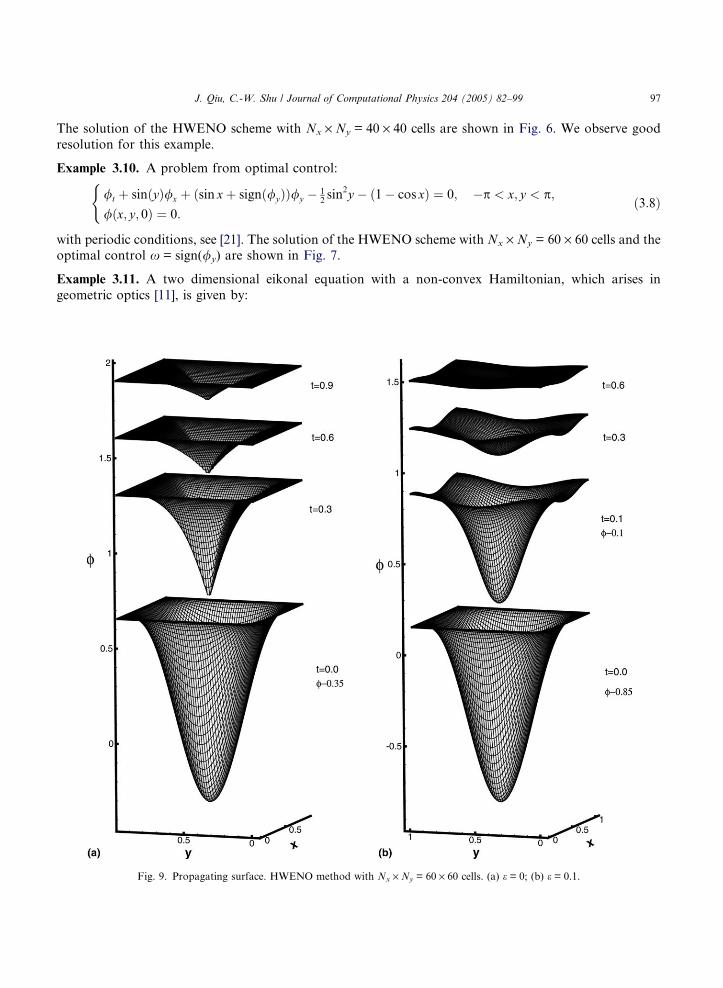
Example 3.11. A two dimensional eikonal equation with a non-convex Hamiltonian, which arises in

geometric optics [11], is given by:

Fig. 9. Propagating surface. HWENO method with Nx · Ny = 60 · 60 cells. (a) e = 0; (b) e = 0.1.


/t þffiffiffiffiffiffiffiffiffiffiffiffiffiffiffiffiffiffiffiffiffiffiffiffiffi/2

x þ /2y þ 1

q¼ 0; 0 6 x; y < 1;

/ðx; y; 0Þ ¼ 14ðcosð2pxÞ � 1Þðcosð2pyÞ � 1Þ � 1:

8<: ð3:9Þ

The solutions of the HWENO scheme with Nx · Ny = 80 · 80 cells is shown in Fig. 8. Good resolution is

observed.

Example 3.12. The problem of a propagating surface [20]:

/t � ð1� eKÞffiffiffiffiffiffiffiffiffiffiffiffiffiffiffiffiffiffiffiffiffiffiffiffiffi/2

x þ /2y þ 1

q¼ 0; 0 6 x; y < 1;

/ðx; y; 0Þ ¼ 1� 14ðcosð2pxÞ � 1Þðcosð2pyÞ � 1Þ;

8<: ð3:10Þ

where K is the mean curvature defined by

K ¼ �/xxð1þ /2

yÞ � 2/xy/x/y þ /yyð1þ /2xÞ

ð1þ /2x þ /2

yÞ3=2

:

and e is a small constant. A periodic boundary condition is used. The approximation of the second deriv-

ative terms are constructed by the methods similar to that of the first derivative terms, but we only uselinear weights in the reconstruction. The results of e = 0 (pure convection) and e = 0.1 by the HWENO

method with Nx · Ny = 60 · 60 cells are presented in Fig. 9. The surfaces at t = 0 for e = 0 and for

e = 0.1, and at t = 0.1 for e = 0.1, are shifted downward in order to show the detail of the solution at later

time.

4. Concluding remarks

In this paper, we have constructed a new class of fifth order WENO schemes, which we called the

HWENO (Hermite WENO) schemes, for solving one and two dimensional Hamilton–Jacobi equations.

The construction of HWENO schemes for Hamilton–Jacobi equations is based on Hermite interpolationand Runge–Kutta methods. The idea of the reconstruction for the HWENO schemes comes from the

WENO schemes. In the HWENO schemes, both the solution and its first derivatives are evolved in time

and used in the reconstruction, in contrast to the regular WENO schemes where only the solution value

is evolved in time and used in the reconstruction. Comparing with the regular WENO schemes, one major

advantage of HWENO schemes is their relatively compact stencil. Extensive numerical experiments are

performed to illustrate the capability of the method.

Acknowledgements

The first author thank Professor B.C. Khoo and Professor G.W. Wei for their support and help.

References

[1] S. Augoula, R. Abgrall, High order numerical discretization for Hamilton–Jacobi equations on triangular meshes, J. Sci. Comput.

15 (2000) 198–229.

[2] F. Bouchut, C. Bourdarias, B. Perthame, A MUSCL method satisfying all the numerical entropy inequalities, Math. Comput. 65

(1996) 1439–1461.


[3] S. Bryson, D. Levy, High-order semi-discrete central-upwind schemes for multi-dimensional Hamilton–Jacobi equations, J.

Comput. Phys. 189 (2003) 63–87.

[4] S. Bryson, D. Levy, High-order central WENO schemes for multidimensional Hamilton–Jacobi equations, SIAM J. Numer. Anal.

41 (2003) 1339–1369.

[5] T.J. Barth, J.A. Sethian, Numerical schemes for the Hamilton–Jacobi and level set equations on triangulated domains, J. Comput.

Phys. 145 (1998) 1–40.

[6] T. Cecil, J. Qian, S. Osher, Numerical methods for high dimensional Hamilton–Jacobi equations using radial basis functions, J.

Comput. Phys. 196 (2004) 327–347.

[7] R.L. Dougherty, A.S. Edelman, J.M. Hyman, Nonnegativity-, monotonicity- or convexity-preserving cubic and quintic Hermite

interpolation, Math. Comput. 52 (1989) 471–494.

[8] O. Friedrichs, Weighted essentially non-oscillatory schemes for the interpolation of mean values on unstructured grids, J. Comput.

Phys. 144 (1998) 194–212.

[9] A. Harten, B. Engquist, S. Osher, S. Chakravathy, Uniformly high order accurate essentially non-oscillatory schemes, III, J.

Comput. Phys. 71 (1987) 231–303.

[10] C. Hu, C.-W. Shu, A discontinuous Galerkin finite element method for Hamilton–Jacobi equations, SIAM J. Sci. Comput. 21

(1999) 666–690.

[11] S. Jin, Z. Xin, Numerical passage from systems of conservation laws to Hamilton–Jacobi equations, and relaxation schemes,

SIAM J. Numer. Anal. 35 (1998) 2163–2186.

[12] G. Jiang, D. Peng, Weighted ENO schemes for Hamilton–Jacobi equations, SIAM J. Sci. Comput. 21 (2000) 2126–2143.

[13] G. Jiang, C.-W. Shu, Efficient implementation of weighted ENO schemes, J. Comput. Phys. 126 (1996) 202–228.

[14] A. Kurganov, E. Tadmor, New high-resolution semi-discrete central schemes for Hamilton–Jacobi equations, J. Comput. Phys.

160 (2000) 720–742.

[15] F. Lafon, S. Osher, High order two dimensional nonoscillatory methods for solving Hamilton–Jacobi scalar equations, J.

Comput. Phys. 123 (1996) 235–253.

[16] O. Lepsky, C. Hu, C.-W. Shu, Analysis of the discontinuous Galerkin method for Hamilton–Jacobi equations, Appl. Numer.

Math. 33 (2000) 423–434.

[17] D. Levy, G. Puppo, G. Russo, Central WENO schemes for hyperbolic systems of conservation laws, Math. Model. Numer. Anal.

33 (1999) 547–571.

[18] X. Liu, S. Osher, T. Chan, Weighted essentially non-oscillatory schemes, J. Comput. Phys. 115 (1994) 200–212.

[19] T. Nakamura, R. Tanaka, T. Yabe, K. Takizawa, Exactly conservative semi-Lagrangian scheme for multi-dimensional

hyperbolic equations with directional splitting technique, J. Comput. Phys. 174 (2001) 171–207.

[20] S. Osher, J. Sethian, Fronts propagating with curvature dependent speed: algorithms based on Hamilton–Jacobi formulations, J.

Comput. Phys. 79 (1988) 12–49.

[21] S. Osher, C.-W. Shu, High-order essentially nonoscillatory schemes for Hamilton–Jacobi equations, SIAM J. Numer. Anal. 28

(1991) 907–922.

[22] J. Qiu, C.-W. Shu, On the construction, comparison, local characteristic decomposition for high order central WENO schemes, J.

Comput. Phys. 183 (2002) 187–209.

[23] J. Qiu, C.-W. Shu, Hermite WENO schemes and their application as limiters for Runge–Kutta discontinuous Galerkin method:

one dimensional case, J. Comput. Phys. 193 (2003) 115–135.

[24] J. Qiu, C.-W. Shu, Hermite WENO schemes and their application as limiters for Runge–Kutta discontinuous Galerkin method II:

two dimensional case, Comp. Fluid (in press).

[25] C.-W. Shu, Essentially non-oscillatory and weighted essentially non-oscillatory schemes for hyperbolic conservation laws, in: B.

Cockburn, C. Johnson, C.-W. Shu, E. Tadmor (Eds.), Advanced Numerical Approximation of Nonlinear Hyperbolic Equations,

A. Quarteroni (Ed.), Lecture Notes in Mathematics, vol. 1697, Springer, Berlin, 1998, pp. 325–432.

[26] C.-W. Shu, S. Osher, Efficient implementation of essentially non-oscillatory shock-capturing schemes, J. Comput. Phys. 77 (1988)

439–471.

[27] C.-W. Shu, S. Osher, Efficient implementation of essentially non-oscillatory shock capturing schemes II, J. Comput. Phys. 83

(1989) 32–78.

[28] H. Takewaki, A. Nishiguchi, T. Yabe, Cubic interpolated pseudoparticle method (CIP) for solving hyperbolic type equations, J.

Comput. Phys. 61 (1985) 261–268.

[29] Y.-T. Zhang, C.-W. Shu, High-order WENO schemes for Hamilton–Jacobi equations on triangular meshes, SIAM J. Sci.

Comput. 24 (2003) 1005–1030.

hermite weno schemes for hamilton–jacobi...

Documents