high-order central weno schemes for multi-dimensional ... · pdf filehigh-order central weno...

High-Order Central WENO Schemes for

Multi-Dimensional Hamilton-Jacobi Equations

Steve Bryson∗ Doron Levy†

July 11, 2002

Abstract

We present new third- and fifth-order Godunov-type central schemes for ap-proximating solutions of the Hamilton-Jacobi (HJ) equation in an arbitrary num-ber of space dimensions. These are the first central schemes for approximatingsolutions of the HJ equations with an order of accuracy that is greater than two.In two space dimensions we present two versions for the third-order scheme: onescheme that is based on a genuinely two-dimensional Central WENO reconstruc-tion, and another scheme that is based on a simpler dimension-by-dimension re-construction. The simpler dimension-by-dimension variant is then extended to amulti-dimensional fifth-order scheme. Our numerical examples in one, two andthree space dimensions verify the expected order of accuracy of the schemes.

Key words. Hamilton-Jacobi equations, central schemes, high order, WENO, CWENO.

AMS(MOS) subject classification. Primary 65M06; secondary 35L99.

Contents

1 Introduction 2

2 One-Dimensional Schemes 42.1 One-Dimensional Central Schemes . . . . . . . . . . . . . . . . . . . . . . 42.2 A Third-Order Scheme . . . . . . . . . . . . . . . . . . . . . . . . . . . . 62.3 A Fifth-Order Scheme . . . . . . . . . . . . . . . . . . . . . . . . . . . . 10∗Program in Scientific Computing/Computational Mathematics, Stanford University and the NASA

Advanced Supercomputing Division, NASA Ames Research Center, Moffett Field, CA 94035-1000;[email protected]

†Department of Mathematics, Stanford University, Stanford, CA 94305-2125;[email protected]

1

2 S. Bryson and D. Levy

3 Multi-Dimensional Schemes 133.1 Two-Dimensional Central Schemes . . . . . . . . . . . . . . . . . . . . . 133.2 Two-Dimensional Third-Order Schemes . . . . . . . . . . . . . . . . . . . 16

3.2.1 A two-dimensional reconstruction of ϕi±α,j±α . . . . . . . . . . . . 163.2.2 A dimension-by-dimension reconstruction of ϕi±α,j±α . . . . . . . 203.2.3 The reprojection step . . . . . . . . . . . . . . . . . . . . . . . . . 20

3.3 A Two-Dimensional Fifth-Order Scheme . . . . . . . . . . . . . . . . . . 233.4 Multi-Dimensional Extensions . . . . . . . . . . . . . . . . . . . . . . . . 25

4 Numerical Simulations 254.1 One-Dimensional Examples . . . . . . . . . . . . . . . . . . . . . . . . . 254.2 Two-Dimensional Examples . . . . . . . . . . . . . . . . . . . . . . . . . 314.3 A Comparison of Two-Dimensional Third-Order Interpolants . . . . . . . 354.4 A Stability Study . . . . . . . . . . . . . . . . . . . . . . . . . . . . . . . 364.5 Three-Dimensional Examples . . . . . . . . . . . . . . . . . . . . . . . . 40

1 Introduction

We are interested in high-order numerical approximations for the solution of multi-dimensional Hamilton-Jacobi (HJ) equations of the form

φt + H(∇φ) = 0, ~x = (x1, . . . xd) ∈ Rd,

where H is the Hamiltonian, which we assume depends on ∇φ and possibly on x and t.In recent years, the HJ equations attracted a lot of attention from analysts and numericalanalysts due to the important role that they play in applications such as optimal controltheory, image processing, geometric optics, differential games, calculus of variations, etc.The main difficulty in treating these equations is due to the discontinuous derivativesthat develop in finite time even when the initial data is smooth. Vanishing viscositysolutions provide a good tool for defining weak solutions when the Hamiltonian is convex[15]. The celebrated viscosity solution provides a suitable extension of weak solutionsfor more general Hamiltonians [3, 7, 8, 9, 10, 28, 29].

Given the importance of the HJ equations, there has been relatively little activitydeveloping numerical tools for approximating their solutions. This is surprising giventhat most of the numerical ideas are based in the similarity between hyperbolic conser-vation laws and the HJ equations, and the field of numerical methods for conservationlaws has been flourishing in recent years.

Converging first-order approximations were introduced by Souganidis in [38]. High-order upwind methods were introduced by Osher, Sethian and Shu in [34, 35]. Thesemethods are based on Harten’s Essentially Non-Oscillatory (ENO) reconstruction [13],

High Order Schemes for HJ Equations 3

that is evolved in time with a first-order monotone flux. The Weighted ENO (WENO)interpolant of [18, 32] was used for constructing high-order upwind methods for the HJequations in [17], and extensions of these methods for triangular meshes were introducedin [1, 40]. We note in passing that there are other approaches for approximating solutionsof HJ equation such as discontinuous Galerkin methods [14, 24] and relaxation schemes[20].

A different class of Godunov-type schemes for hyperbolic conservation laws, the so-called “central schemes”, have recently been applied to the HJ equations. The prototypefor these schemes is the Lax-Friedrichs scheme [11]. A second-order staggered centralscheme was developed for conservation laws by Nessyahu and Tadmor in [33]. Themain advantage of central schemes is their simplicity. Since they do not require any(approximate) Riemann solvers, they are particularly suitable for approximating multi-dimensional systems of conservation laws. Lin and Tadmor applied these ideas to the HJequations in [31]. There, first- and second-order staggered schemes versions of [2, 19, 33]were written in one and two space dimensions. An L1 convergence of order one for thisscheme was proved in [30]. After the introduction of a semi-discrete central schemefor hyperbolic conservation laws in [23], a second-order semi-discrete scheme for HJequations was introduced by the same authors in [22]. While less dissipative, this schemerequires the estimation of the local speed of propagation at every grid point, a task thatis computationally intensive in particular with problems of high dimensionality. Byconsidering more precise information about the local speed of propagation, an even lessdissipative scheme was generated in [21].

Recently we introduced in [5] new and efficient central schemes for multi-dimensionalHJ equations. These non-oscillatory, non-staggered schemes were first- and second-orderaccurate and were designed to scale well with an increasing dimension. Efficiency wasobtained by carefully choosing the location of the evolution points and by using a one-dimensional projection step. Avoiding staggering by adding an additional projectionstep is an idea which we already utilized in the framework of conservation laws [16].

In this work we introduce third- and fifth-order accurate schemes for approximatingsolutions of multi-dimensional HJ equations. These are the first central schemes for suchequations of order greater than two. This work is the HJ analog to the correspondingworks in conservation laws: an ENO based central scheme [4], and the Central WENO(CWENO) central schemes [25, 26, 27]. We announced a preliminary version of the onedimensional results in a recent proceedings publication [6].

The structure of this paper is as follows. We start in §2 with the derivation of ourone-dimensional schemes. A third-order WENO reconstruction scheme is presented in§2.2. This scheme required a fourth-order reconstruction of the point-values and a third-order reconstruction of the derivatives at the evolution points. Even though the optimallocation of the evolution points in one dimension is in the center of the interval, in orderto prepare the grounds for the multi-dimensional schemes we write a reconstruction for


an arbitrary location of the evolution points. A fifth-order method is then presented in§2.3.

We turn to the multi-dimensional framework in §3. Here there is flexibility in thereconstruction step. For simplicity we carry most of the discussion in two space di-mensions. Extensions to more than two space dimensions are presented in §3.4. First,we provide a brief outline of the general structure of two-dimensional central schemesin §3.1. The main remaining ingredient, the reconstruction step, is then described inthe following two sections. For a two-dimensional third-order scheme we present in§3.2 two ways to obtain a high-order reconstruction of the approximate solution at theevolution points. The first option in §3.2.1 is based on a genuinely two-dimensional re-construction. An alternative dimension-by-dimension approach is based on a sequenceof one-dimensional reconstructions and is presented in §3.2.2. Our numerical resultsshow that both approaches are essentially equivalent. Hence, the rest of the paper dealswith the dimension-by-dimension reconstruction. A fifth-order dimension-by-dimensionextension of the one-dimensional scheme in §2.3 to two dimensions is then presented in§3.3. Since the solution at the next time step is computed at grid points that are differ-ent from those on which the data is given, we reproject the evolved solution back ontothe original grid points. Different ways to approach this reprojection step are discussedin §3.2.3.

We conclude in §4 with several numerical examples in one, two and three spacedimensions that confirm the expected order of accuracy and the high-resolution natureof our scheme. We compare our results with the scheme of Jiang and Peng in [17]. Wealso study the convergence rate after the emergence of the discontinuities in the solution.

Acknowledgment: We would like to thank Volker Elling for helpful discussions through-out the early stages of this work. The work of D. Levy was supported in part by theNational Science Foundation under Career Grant No. DMS-0133511.

2 One-Dimensional Schemes

2.1 One-Dimensional Central Schemes

Consider the one-dimensional Hamilton-Jacobi equation of the form

φt(x, t) + H (φx) = 0, x ∈ R. (2.1)

We are interested in approximating solutions of (2.1) subject to the initial data φ(x, t=0) = φ0(x). For simplicity we assume a uniform grid grid in space and time with meshspacings, ∆x and ∆t, respectively. Denote the grid points by xi = i∆x, tn = n∆t, andthe fixed mesh ratio by λ = ∆t/∆x. Let ϕn

i denote the approximate value of φ (xi, tn),


and (ϕx)ni denote the approximate value of the derivative φx (xi, t

n). We define theforward and backward differencing as ∆+ϕn

i := ϕni+1 − ϕn

i and ∆−ϕni := ϕn

i − ϕni−1.

Assume that the approximate solution at time tn, ϕni is given. A Godunov-type

scheme for approximating the solution of (2.1) starts with a continuous piecewise-polynomial ϕ(x, tn) that is reconstructed from the data, ϕn

i ,

ϕ(x, tn) =∑

i

Pi+ 1

2

(x, tn)χi+ 1

2

(x). (2.2)

Here, χi+1/2(x) is the characteristic function of the interval [xi, xi+1], and Pi+1/2(x, tn)is a polynomial of a suitable degree that satisfies the interpolation requirements

Pi+ 1

2

(xi+β, tn) = ϕni+β, β = 0, 1.

The reconstruction (2.2) is then evolved from time tn to time tn+1 according to (2.1),and sampled at the half-integer grid-points, {xi+1/2}, where the reconstruction is smooth(as long as the CFL condition λ |H ′ (ϕx)| ≤ 1/2 is satisfied)

ϕn+1i+ 1

2

= ϕni+ 1

2

−∫ tn+1

tnH(

ϕx

(

xi+ 1

2

, τ))

dτ. (2.3)

The point-value ϕni+1/2 is obtained by sampling (2.2), at xi+1/2, i.e. ϕn

i+1/2 = ϕ(xi+1/2, tn).

Since the evolution step (2.3) is done at points where the solution is smooth, we can ap-proximate the time integral at the RHS of (2.3) using a sufficiently accurate quadraturerule. For example, for a third- and fourth-order method, this integral can be replacedby a Simpson’s quadrature,

∫ tn+1

tnH(

ϕx

(

xi+ 1

2, τ))

dτ ≈ ∆t

6

[

H(

ϕ′ ni+ 1

2

)

+ 4H(

ϕ′ n+ 1

2

i+ 1

2

)

+ H(

ϕ′ n+1i+ 1

2

)]

. (2.4)

The derivative at time tn, ϕ′ ni+1/2 is obtained by sampling the derivative of the recon-

struction (2.2), i.e., ϕ′ ni+1/2 = ϕ′(xi+1/2, t

n). The intermediate values of the derivative in

time, ϕ′ n+1/2i+1/2 , and ϕ′ n+1

i+1/2, which are required in the quadrature (2.4), can be predicted

using a Taylor expansion or with a Runge-Kutta (RK) method. Alternatively, (2.1) canbe treated as a semi-discrete equation by replacing the spatial derivatives with theirnumerical approximations and integrating in time via an RK method.

The only remaining ingredient to specify is the reconstruction (2.2). Below wepresent two reconstructions. The first is a fourth-order reconstruction of the point-values and the derivatives which leads to a third-order scheme, and the second is asixth-order reconstruction that results in a fifth-order scheme.

Remarks.


1. In order to return to the original grid, we project ϕn+1i+1/2 back onto the integer

grid points {xi} to end up with ϕn+1i . This projection is accomplished with the

same reconstruction used to approximate ϕni+1/2 from ϕn

i .

2. In order to maximize the size of the time-step, the evolution points should betaken as far as possible from the singularities in the reconstructedpiecewise-polynomial. In one dimension the appropriate evolution point islocated at xi+1/2. In d-dimensions with a uniform grid with spacing ∆x, theoptimal evolution points are located at xi+α = xi + α∆x in each direction, where

α = 1/(

d +√

d)

(see [5]). One of the multi-dimensional schemes we present in

§3 is based on one-dimensional reconstructions. Hence, in order to prepare thegrounds for the multi-dimensional setup, we write the one-dimensionalreconstruction in this section assuming that the evolution points are xi±α. Thereader should keep in mind that in one dimension, α = 1/2.

3. We would like to point out that one does not need to fully reconstruct thepolynomials Pi+1/2(x, tn). The only values that the scheme requires are theapproximated point-values ϕn

i+1/2 = ϕ(xi+1/2, tn) and the approximated

derivatives ϕ′i+1/2 = ϕ′(xi+1/2). Hence, in the rest of the paper whenever we referto reconstruction steps we directly treat the recovery of these two quantities.

2.2 A Third-Order Scheme

A third-order scheme is generated by combining a third-order accurate ODE solver intime for predicting the intermediate values of the derivatives in (2.4), with a sufficientlyhigh-order reconstruction in space.

Given ϕni , in order to invoke (2.3), we should compute two quantities in every time

step: the point-values at the evolution points, ϕi±α, and the derivative ϕ′i±α. In order toobtain a third-order scheme, the approximations of the point-values should be fourth-order accurate, and the approximation of the derivatives should be third-order accurate.In this scheme, the reconstruction of the point-values is done in locations that arestaggered with respect to the location of the data. The reconstruction of the derivatives,which is required in every step of the ODE solver, is done at the same points wherethe data is given. Since we anyhow need two types of reconstructions and due tosymmetry considerations, we derive a fourth-order approximation of the derivatives.Obviously, this more accurate reconstruction of the derivatives does not increase theorder of accuracy of the scheme but it does reduce the error.

1. The reconstruction of ϕi±α from ϕi


xi xi+α xi+1xi-1 xi+2

+,i+αϕ

-,i+αϕ

Figure 2.1: The two interpolants used for the third-order reconstruction at the evolutionpoint at xi+α.

A fourth-order reconstruction of ϕi+α can be obtained by considering a convexcombination of two quadratic polynomials, each of which requires the evaluationof ϕ on a three-point stencil. One quadratic polynomial ϕ−(x) is constructedon a stencil that is left-biased with respect to xi+α, {xi−1, xi, xi+1}, while theother polynomial ϕ+(x) is constructed on a right-biased stencil, {xi, xi+1, xi+2},see Figure 2.1. We set

ϕ−,i+α =

(−α + α2

2

)

ϕi−1 +(

1− α2)

ϕi +

(

α + α2

2

)

ϕi+1, (2.5)

ϕ+,i+α =

(

2− 3α + α2

2

)

ϕi +(

2α− α2)

ϕi+1 +

(−α + α2

2

)

ϕi+2.

For smooth ϕ, a straightforward computation shows that ϕ±,i+α = ϕ (xi+α) +O (∆x3), and

1

3(2− α)ϕ−,i+α +

1

3(1 + α)ϕ+,i+α = ϕ (xi+α) + O

(

∆x4)

.

Similarly, the reconstruction of ϕi−α is obtained using the quadratic polynomialsϕ−(x) based on the left-biased stencil enclosing xi−α, {xi−2, xi−1, xi}, and ϕ+(x)based on the right biased stencil {xi−1, xi, xi+1},

ϕ−,i−α =

(−α + α2

2

)

ϕi−2 +(

2α− α2)

ϕi−1 +

(

2− 3α + α2

2

)

ϕi, (2.6)

ϕ+,i−α =

(

α + α2

2

)

ϕi−1 +(

1− α2)

ϕi +

(−α + α2

2

)

ϕi+1.


This time, ϕ±,i−α = ϕ (xi−α) + O (∆x3), and

1

3(1 + α)ϕ−,i−α +

1

3(2− α)ϕ+,i−α = ϕ (xi−α) + O

(

∆x4)

.

A fourth-order WENO estimate of ϕi±α is therefore given by the convex combina-tion

ϕi±α = w−i±αϕ−,i±α + w+

i±αϕ+,i±α, (2.7)

where the weights satisfy w−i±α + w+

i±α = 1, w±i±α ≥ 0, ∀i. In smooth regions we

would like to satisfy w−i+α = w+

i−α ≈ (2− α) /3 and w+i+α = w−

i−α ≈ (1 + α) /3to attain an O (∆x4) error. When the stencil supporting ϕi±α contains a discon-tinuity, the weight of the more oscillatory polynomial should vanish. Following[18, 32], these requirements are met by setting

wki±α =

αki±α

∑

l αli±α

, αki±α =

cki±α

(

ε + Ski±α

)p , (2.8)

where k, l ∈ {+,−}. The constants are independent of the grid index i and aregiven by c−i+α = c+

i−α = (2− α) /3, c+i+α = c−i−α = (1 + α) /3. We choose ε as 10−6

to prevent the denominator in (2.8) from vanishing, and set p = 2 (see [18]). Thesmoothness measures S±i should be large when ϕ is nearly singular. Following[18], we take Si±α to be the sum of the L2-norms of the derivatives on the stencilsupporting ϕ±. If we approximate the first derivative at xi by ∆+ϕi/∆x, thesecond derivative by ∆+∆−ϕi±α/(∆x)2, and define the smoothness measure

Si [r, s] = ∆xs∑

j=r

(

1

∆x∆+ϕi+j

)2

+ ∆xs∑

j=r+1

(

1

∆x2∆+∆−ϕi+j

)2

, (2.9)

then we have S−i+α = Si [−1, 0], S+i+α = Si [0, 1], S−i−α = Si [−2,−1] and S+

i−α =Si [−1, 0].

For future reference we label the reconstruction in this section with the proceduralform

ϕi±α = reconstruct ϕ 1D 3 (i,±α, ϕ) , (2.10)

where ϕ is the one-dimensional array (ϕ1, . . . , ϕN). This notation will be used inthe dimension-by-dimension reconstructions in §3.


2. The reconstruction of ϕ′i±α from ϕi±α

The values of ϕ we recovered in the previous step at the regularly spaced lo-cations {xi±α} can be used to recover the derivative ϕ′i±α via a (non-central)WENO reconstruction. To obtain a fourth-order WENO approximation of ϕ′i±α,we write a convex combination of three quadratic interpolants: ϕ′−,i±α on the sten-cil {xi−2±α, xi−1±α, xi±α}, ϕ′0,i±α on the stencil {xi−1±α, xi±α, xi+1±α} and ϕ′+,i±α

on the stencil {xi±α, xi+1±α, xi+2±α}. For smooth ϕ,

ϕ′−,i±α =1

2∆x(ϕi−2±α − 4ϕi−1±α + 3ϕi±α) = ϕ′ (xi±α) + O

(

∆x3)

,

ϕ′0,i±α =1

2∆x(ϕi+1±α − ϕi−1±α) = ϕ′ (xi±α) + O

(

∆x3)

, (2.11)

ϕ′+,i±α =1

2∆x(−3ϕi±α + 4ϕi+1±α − ϕi+2±α) = ϕ′ (xi±α) + O

(

∆x3)

.

A straightforward computation yields

1

6ϕ′−,i±α +

2

3ϕ′0,i±α +

1

6ϕ′+,i±α = ϕ′ (xi±α) + O

(

∆x4)

.

The fourth-order WENO estimate of ϕ′i±α from ϕi±α is therefore

ϕ′i±α = w−i±αϕ′−,i±α + w0

i±αϕ′0,i±α + w+i±αϕ′+,i±α, (2.12)

where the weights w are of the form (2.8) with k, l ∈ {+, 0,−}, c− = c+ = 1/6, c0 =2/3, and the oscillatory indicators are S−i±α = Si±α [−2,−1], S0

i±α = Si±α [−1, 0],and S+

i±α = Si±α [0, 1].

For future reference we label the above reconstruction of ϕ′i±α with the proceduralform

ϕ′i±α = reconstruct ϕ′ 1D 3 (i,±α, ϕ±α) , (2.13)

where ϕ±α is the one-dimensional array (ϕ1±α, . . . , ϕN±α).

We would like to summarize the one-dimensional third-order algorithm in the follow-ing, where RK

(

ϕni±α, ϕ′ n

i±α, ∆t)

is the third-order Runge-Kutta method which integrates(2.1) and is used to predict the intermediate values of the derivatives. Each internalstep of the RK method will require additional reconstructions of ϕ′i±α from that step’sϕi±α.

Algorithm 2.1 Assume that {ϕni } are given.


1. Reconstruct:

ϕni±α = reconstruct ϕ 1D 3 (i,±α, ϕn)

ϕ′ ni±α = reconstruct ϕ′ 1D 3

(

i,±α, ϕni±α

)

2. Integrate:

ϕn+ 1

2

i±α = RK(

ϕni±α, ϕ′ n

i±α, ∆t/2)

ϕ′ n+ 1

2

i±α = reconstruct ϕ′ 1D 3(

i,±α, ϕn+ 1

2

i±α

)

ϕn+1i±α = RK

(

ϕni±α, ϕ′ n

i±α, ∆t)

ϕ′ n+1i±α = reconstruct ϕ′ 1D 3

(

i,±α, ϕn+1i±α

)

ϕn+1i±α = ϕn

i±α +∆t

6

[

H(

ϕ′ ni±α

)

+ 4H(

ϕ′ n+ 1

2

i±α

)

+ H(

ϕ′ n+1i±α

)

]

.

3. Reproject:

ϕn+1i = reconstruct ϕ 1D 3

(

i,∓α, ϕn+1i±α

)

.

Remark. It is possible to replace the Simpson’s quadrature in the integration step witha single RK time-step, ϕn+1

i±α = RK(

ϕni±α, ϕ′ n

i±α, ∆t)

. Our simulations show that thischoice reduces the complexity of the computation but also reduces its accuracy.

2.3 A Fifth-Order Scheme

In order to obtain a fifth-order scheme, we need a sixth-order approximation of thepoint-values of ϕ, a fifth-order approximation of the derivative ϕ′, and a higher-orderprediction of the intermediate derivatives which appear in the quadrature formula. Dueto arguments similar to those given in §2.2, we again derive a more accurate reconstruc-tion of the derivatives, which in this case is sixth-order.

We start with the reconstruction of ϕi+α from ϕi. We write sixth-order interpolantsas a convex combination of three cubic interpolants, each of which requires the evaluationof ϕ on a four-point stencil. We use the polynomials ϕ−(x) defined on the left-biasedstencil {xi−2, xi−1, xi, xi+1}, ϕ0(x) defined on the centered stencil {xi−1, xi, xi+1, xi+2}


xi xi+α xi+1xi-1 xi+2

0ϕ

xi+3xi-2

-ϕ

+ϕ

Figure 2.2: The three interpolants used for the fifth-order reconstruction ϕi+α at theevolution point at xi+α. In this example, because of the large gradient between xi+1

and xi+2, the interpolant ϕ− will have the strongest contribution to the CWENO recon-struction at xi+α.

and ϕ+(x) defined on the right-biased stencil {xi, xi+1, xi+2, xi+3}, see Figure 2.2. Forsmooth ϕ

ϕ−,i+α = a1ϕi−2 + a2ϕi−1 + a3ϕi + a4ϕi+1 = ϕ (xi+α) + O(

∆x4)

, (2.14)

ϕ0,i+α = a5ϕi−1 + a6ϕi + a7ϕi+1 + a8ϕi+2 = ϕ (xi+α) + O(

∆x4)

,

ϕ+,i+α = a9ϕi + a10ϕi+1 + a11ϕi+2 + a12ϕi+3 = ϕ (xi+α) + O(

∆x4)

,

where the constants are given by

a1 =1

6α− 1

6α3, a2 = −α +

1

2α2 +

1

2α3,

a3 = 1 +1

2α− α2 − 1

2α3, a4 =

1

3α +

1

2α2 +

1

6α3,

a5 = −1

3α +

1

2α2 − 1

6α3, a6 = 1− 1

2α− α2 +

1

2α3,

a7 = α +1

2α2 − 1

2α3, a8 = −1

6α +

1

6α3 = −a1,

a9 = 1− 11

6α + α2 − 1

6α3, a10 = 3α− 5

2α2 +

1

2α3,

a11 = −3

2α + 2α2 − 1

2α3, a12 =

1

3α− 1

2α2 +

1

6α3.

At xi−α we have

ϕ−,i−α = a12ϕi−3 + a11ϕi−2 + a10ϕi−1 + a9ϕi = ϕ (xi−α) + O(

∆x4)

, (2.15)

ϕ0,i−α = a8ϕi−2 + a7ϕi−1 + a6ϕi + a5ϕi+1 = ϕ (xi−α) + O(

∆x4)

,

ϕ+,i−α = a4ϕi−1 + a3ϕi + a2ϕi+1 + a1ϕi+2 = ϕ (xi−α) + O(

∆x4)

.

A straightforward computation yields

c−i±αϕ−,i±α + c0i±αϕ0,i±α + c+

i±αϕ+,i±α = ϕ (xi±α) + O(

∆x6)

,


where

c−i+α = c+i−α =

1

20α2 − 1

4α +

3

10, (2.16)

c0i±α = − 1

10α2 +

1

10α +

3

5,

c+i+α = c−i−α =

1

20α2 +

3

20α +

1

10.

A sixth-order reconstruction of ϕi±α is therefore given by

ϕi±α = w−i±αϕ−,i±α + w0

i±αϕ0,i±α + w+i±αϕ+,i±α, (2.17)

where the weights wk are given by (2.8) with k, l ∈ {+, 0,−}, and the constants ck

are given by (2.16). The oscillatory indicators are given via (2.9) by S−i±α = Si [−2, 0],

S0i±α = Si [−1, 1] and S+

i±α = Si [0, 2].A sixth-order approximation of ϕ′i±α from ϕi±α is written as a convex combination

of four cubic interpolants. This reconstruction is similar to the third-order case, and isbased on a non-central WENO reconstruction. We skip the details and summarize theresult:

ϕ′i±α = w1i±αϕ′1,i±α + w2

i±αϕ′2,i±α + w3i±αϕ′3,i±α + w4

i±αϕ′4,i±α, (2.18)

where

ϕ′1,i±α =1

6∆x(−2ϕi−3±α + 9ϕi−2±α − 18ϕi−1±α + 11ϕi±α),

ϕ′2,i±α =1

6∆x(ϕi−2±α − 6ϕi−1±α + 3ϕi±α + 2ϕi+1±α),

ϕ′3,i±α =1

6∆x(−2ϕi−1±α − 3ϕi±α + 6ϕi+1±α − ϕi+2±α),

ϕ′4,i±α =1

6∆x(−11ϕi±α + 18ϕi+1±α − 9ϕi+2±α + 2ϕi+3±α).

Here the weights wk are given by (2.8) with c1 = c4 = 1/20, c2 = c3 = 9/20, S1i±α =

Si±α [−3,−1], S2i±α = Si±α [−2, 0], S3

i±α = Si±α [−1, 1] and S4i±α = Si±α [0, 2].

Notations.

1. We label the reconstruction of the point-values (2.17) as

ϕi±α = reconstruct ϕ 1D 5 (i,±α, ϕ) , (2.19)

where ϕ is the one-dimensional array (ϕ1, . . . , ϕN).


2. We label the reconstruction of ϕ′i±α (2.18) as

ϕ′i±α = reconstruct ϕ′ 1D 5 (i,±α, ϕ±α) , (2.20)

where ϕ±α is the one-dimensional array (ϕ1±α, . . . , ϕN±α).

Remarks.

1. To conclude, the fifth-order method is given by Algorithm 2.1, where thefourth-order reconstructions are replaced by the sixth-order reconstructions(2.19)–(2.20). As is, this scheme is only fourth-order in time. A higher ordermethod in time can be easily obtained by replacing Simpson’s quadrature with amore accurate quadrature and computing the sixth-order approximations for thepoint-values and the derivatives at the new quadrature points.

2. We choose to predict the intermediate values of the derivatives in time using thefourth-order strong stability preserving (SSP) Runge-Kutta scheme of [12]. Fors ∈

{

12, 1}

, the SSP-RK scheme is given by

ϕ(1) = ϕn − 1

2s∆tH (ϕn

x) ,

ϕ(2) =649

1600ϕn +

10890423

25193600s∆tH (ϕn

x) +951

1600ϕ(1) − 5000

7873s∆tH

(

ϕ(1)x

)

,

ϕ(3) =53989

2500000ϕn +

102261

5000000s∆tH (ϕn

x) +4806213

20000000ϕ(1)

+5121

20000s∆tH

(

ϕ(1)x

)

+23619

32000ϕ(2) +

7873

10000s∆tH

(

ϕ(2)x

)

,

ϕn+s =1

5ϕn − 1

10s∆tH (ϕn

x) +6127

30000ϕ(1) +

1

6s∆tH

(

ϕ(1)x

)

+7873

30000ϕ(2)

+1

3ϕ(3) − 1

6s∆tH

(

ϕ(3)x

)

.

Alternatively, the Natural Continuous Extension of the RK method [39] can be

used to produce the intermediate values ϕ′ n+ 1

2 and ϕ′ n+1 with a single RK step,though we observe that errors are somewhat larger in this case.

3 Multi-Dimensional Schemes

3.1 Two-Dimensional Central Schemes

Consider the two-dimensional HJ equation of the form

φt + H(∇φ) = 0, ~x = (x1, x2) ∈ R2, (3.1)


subject to the initial data φ(~x, t = 0) = φ0(~x). Denote xi,j := (x1 + i∆x1, x2 + j∆x2).Similarly to the one-dimensional setup, ϕi,j will denote the approximation of φ at xi,j.We define the two sets of grid points, I+ = {xi,j, xi+1,j, xi,j+1}, and I− = {xi,j, xi−1,j, xi,j−1},and denote by T+, T− the triangles with vertices I+ and I− respectively. For simplicitywe assume a uniform grid ∆x1 = ∆x2 = ∆x.

Assume that the approximate solution at time tn, ϕni,j is given. Similarly to the one-

dimensional setup in §2.1, a Godunov-type scheme for approximating the solution of(3.1) starts with a continuous piecewise-polynomial ϕ(~x, tn) that is reconstructed fromthe data, ϕn

i,j,

ϕ(~x, tn) =∑

i,j

PT±i,j (~x, tn)χT±(~x). (3.2)

As usual, χT±(~x) is the characteristic function of the triangle T±, and PT±i,j (~x, tn) is a

polynomial of a suitable degree that satisfies the interpolation requirements

PT±i,j (~xl, t

n) = ϕ(~xl, tn), ~xl ∈ I±

(see Figure 3.1). The reconstruction (3.2) is then evolved from time tn to time tn+1

by (3.1), and sampled at the evolution points {xi±α,j±α}. In two dimensions the choiceα = 1/(2 +

√2) guarantees that the solution remains smooth at the evolution point as

long as the CFL condition ∆t∆x|H ′ (∇ϕ)| < α is satisfied. The evolved solution now reads

ϕn+1i±α,j±α = ϕn

i±α,j±α −∫ tn+1

tnH (∇ϕ (xi±α,j±α, τ)) dτ. (3.3)

The point-values ϕni±α,j±α are obtained by sampling (3.2) at xi±α,j±α, i.e., ϕn

i±α,j±α =ϕ(xi±α,j±α, tn). Similarly to the one-dimensional case, the evolution points are in smoothregions and therefore the integral on the RHS of (3.3) can be replaced with a sufficientlyaccurate quadrature such as the Simpson rule (2.4), which leads to a scheme that isfourth-order accurate in time. The derivatives at time tn, ϕ′ n

i±α,j±α are obtained bysampling the derivative of the reconstruction (3.2), i.e., ϕ′ n

i±α,j±α = ϕ′(xi±α,j±α, tn). Theother intermediate values of the derivative in time that are required in the quadrature canbe predicted using a Taylor expansion or with a Runge-Kutta method in an analogousway to the one-dimensional case.

Remarks.

1. We present two different algorithms for constructing ϕi±α,j±α: two-dimensionalinterpolants defined on two-dimensional stencils and a dimension-by-dimensionapproach. We present both algorithms for the third-order scheme and extend thesimpler dimension-by-dimension approach to fifth-order. Our numerical


xi-α,j-α

xi+α,j+α

+T

xi,j

ii-1 i+1

j+1

j

j-1-T

Figure 3.1: The location of the evolution points xi±α,j±α and the domain of definitionof the interpolants ϕi±α,j±α in two dimensions.


simulations in §4 indicate that both reconstructions of ϕi±α,j±α are of acomparable quality. In both approaches, the reconstruction of the derivatives∇ϕi±α,j±α is done dimension-by-dimension.

2. We reproject ϕn+1i+α,j+α and ϕn+1

i−α,j−α back onto the integer grid-points, obtaining

ϕn+1i,j . We present several ways to carry out this reprojection: a genuinely

two-dimensional approach, a dimension-by-dimension strategy and a reprojectionalong the diagonal line through xi−α,j−α and xi+α,j+α.

3.2 Two-Dimensional Third-Order Schemes

In order to obtain a third-order scheme, we need a fourth-order reconstruction of thepoint-values at the evolution points xi±α,j±α.

3.2.1 A two-dimensional reconstruction of ϕi±α,j±α

In this section we present a two-dimensional fourth-order reconstruction of the point-values ϕi±α,j±α. In principle, a two-dimensional cubic interpolant would provide a recon-struction with the desired accuracy. Such an interpolant is based on a ten-point stencil.As usual, solving such a direct interpolation problem is unsatisfactory as spurious os-cillations might develop as a result of the lack of smoothness in the solution. Instead,we generate a two-dimensional fourth-order reconstruction as a convex combination offour quadratic interpolants, each which is based on a six-point stencil. We choose com-pact quadratic interpolants such that the union of all the six-point stencils is a compactten-point stencil. Similarly to any WENO-type reconstruction, when singularities arepresent the six-point stencils containing the singularities are suppressed. In any case,we implicitly assume that the solution is sufficiently resolved such that the singulari-ties in the solution are isolated in the sense that they do not occur along neighboringparallel cell edges. Singularities will in general occur along adjacent cell edges. Thereis a lot of flexibility in choosing the ten-point stencil as well as the different six-pointstencils. Here, for the evolution point xi+α,j+α we choose the ten-point stencil shown inFigure 3.2. We choose to use the four six-point stencils that are shown in Figure 3.3.Obviously, the union of these stencils is the ten-point stencil in Figure 3.2. Furthermore,they all enclose the cell containing the evolution point and they all cross different edgesof the enclosing cell. A singularity along an edge will suppress two of these stencils,while a singularity in a corner will suppress three of these stencils.

Remarks.

1. The stencils for the evolution point at xi−α,j−α are obtained by a rotation of 180degrees of the stencils in Figures 3.2–3.3.


j

j+2

j+1

j-1

i-1 i+2i+1i

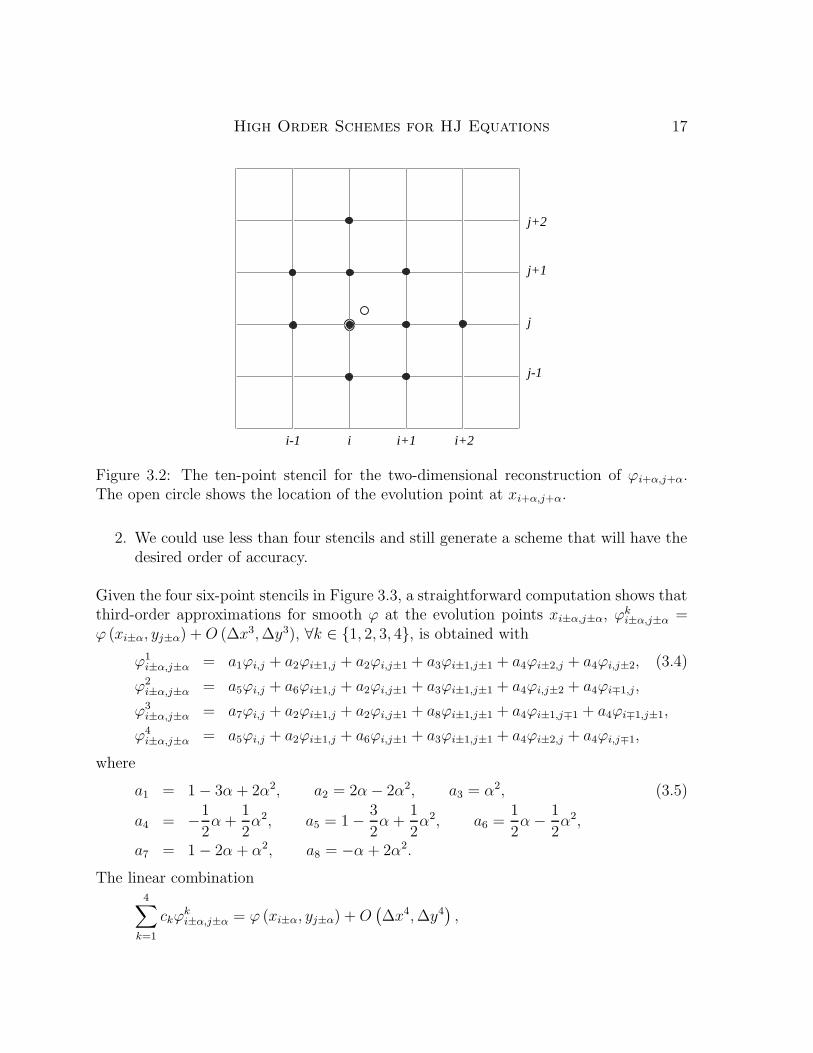
Figure 3.2: The ten-point stencil for the two-dimensional reconstruction of ϕi+α,j+α.The open circle shows the location of the evolution point at xi+α,j+α.

2. We could use less than four stencils and still generate a scheme that will have thedesired order of accuracy.

Given the four six-point stencils in Figure 3.3, a straightforward computation shows thatthird-order approximations for smooth ϕ at the evolution points xi±α,j±α, ϕk

i±α,j±α =ϕ (xi±α, yj±α) + O (∆x3, ∆y3), ∀k ∈ {1, 2, 3, 4}, is obtained with

ϕ1i±α,j±α = a1ϕi,j + a2ϕi±1,j + a2ϕi,j±1 + a3ϕi±1,j±1 + a4ϕi±2,j + a4ϕi,j±2, (3.4)

ϕ2i±α,j±α = a5ϕi,j + a6ϕi±1,j + a2ϕi,j±1 + a3ϕi±1,j±1 + a4ϕi,j±2 + a4ϕi∓1,j,

ϕ3i±α,j±α = a7ϕi,j + a2ϕi±1,j + a2ϕi,j±1 + a8ϕi±1,j±1 + a4ϕi±1,j∓1 + a4ϕi∓1,j±1,

ϕ4i±α,j±α = a5ϕi,j + a2ϕi±1,j + a6ϕi,j±1 + a3ϕi±1,j±1 + a4ϕi±2,j + a4ϕi,j∓1,

where

a1 = 1− 3α + 2α2, a2 = 2α− 2α2, a3 = α2, (3.5)

a4 = −1

2α +

1

2α2, a5 = 1− 3

2α +

1

2α2, a6 =

1

2α− 1

2α2,

a7 = 1− 2α + α2, a8 = −α + 2α2.

The linear combination4∑

k=1

ckϕki±α,j±α = ϕ (xi±α, yj±α) + O

(

∆x4, ∆y4)

,


1 2

3 4

j

j+2

j+1

j-1

i-1 i+2i+1i

j

j+2

j+1

j-1

i-1 i+2i+1i

j

j+2

j+1

j-1

i-1 i+2i+1i

j

j+2

j+1

j-1

i-1 i+2i+1i

Figure 3.3: The four six-point stencils that cover the ten-point stencil for the two-dimensional reconstruction.


is fourth-order accurate provided that the constants ci are taken as

c1 =1

3(5α− 1) , c2 = c4 =

2

3(−2α + 1) , c3 = α. (3.6)

A two-dimensional CWENO reconstruction is a straightforward generalization of theone-dimensional case (compare with (2.7),(2.8)),

ϕi±α,j±α =

4∑

k=1

wki±α,j±αϕk

i±α,j±α.

Here

wki±α,j±α =

αki±α,j±α

∑4l=1 αl

i±α,j±α

, αki±α,j±α =

ck(

ε + Ski±α,j±α

)p ,

with the constants ck given by (3.6). As usual, the smoothness measure for every stencilis taken as a normalized sum of the discrete L2-norms of the derivatives. If we definethe forward and backward differences ∆+

x ϕi,j = ϕi+1,j − ϕi,j, ∆−x ϕi,j = ϕi,j − ϕi−1,j ,

∆+y ϕi,j = ϕi,j+1 − ϕi,j, ∆−

y ϕi,j = ϕi,j − ϕi,j−1, then the smoothness measures for theevolution point xi+α,j+α are given by

S1i+α,j+α =

(

∆+x ϕi,j

)2+(

∆+x ϕi+1,j

)2+(

∆+x ϕi,j+1

)2+(

∆+y ϕi,j

)2+(

∆+y ϕi,j+1

)2

+(

∆+y ϕi+1,j

)2+

1

∆x2

[

(

∆+x ∆−

x ϕi+1,j

)2+(

∆+y ∆−

y ϕi,j+1

)2]

,

S2i+α,j+α =

(

∆+x ϕi,j

)2+(

∆+x ϕi−1,j

)2+(

∆+x ϕi,j+1

)2+(

∆+y ϕi,j

)2+(

∆+y ϕi,j+1

)2

+(

∆+y ϕi+1,j

)2+

1

∆x2

[

(

∆+x ∆−

x ϕi,j

)2+(

∆+y ∆−

y ϕi,j+1

)2]

,

S3i+α,j+α =

(

∆+x ϕi,j

)2+(

∆+x ϕi,j+1

)2+(

∆+x ϕi−1,j+1

)2+(

∆+y ϕi,j

)2+(

∆+y ϕi+1,j

)2

+(

∆+y ϕi+1,j−1

)2+

1

∆x2

[

(

∆+x ∆−

x ϕi,j+1

)2+(

∆+y ∆−

y ϕi+1,j

)2]

,

S4i+α,j+α =

(

∆+x ϕi,j

)2+(

∆+x ϕi+1,j

)2+(

∆+x ϕi,j+1

)2+(

∆+y ϕi,j

)2+(

∆+y ϕi,j−1

)2

+(

∆+y ϕi+1,j

)2+

1

∆x2

[

(

∆+x ∆−

x ϕi+1,j

)2+(

∆+y ∆−

y ϕi,j

)2]

.

The smoothness measures for the evolution point xi−α,j−α are

S1i−α,j−α =

(

∆+x ϕi−2,j

)2+(

∆+x ϕi−1,j

)2+(

∆+x ϕi−1,j−1

)2+(

∆+y ϕi,j−2

)2+(

∆+y ϕi,j−1

)2

+(

∆+y ϕi−1,j−1

)2+

1

∆x2

[

(

∆+x ∆−

x ϕi−1,j

)2+(

∆+y ∆−

y ϕi,j−1

)2]

,

S2i−α,j−α =

(

∆+x ϕi,j

)2+(

∆+x ϕi−1,j

)2+(

∆+x ϕi−1,j−1

)2+(

∆+y ϕi−1,j

)2+(

∆+y ϕi−1,j−1

)2

+(

∆+y ϕi,j−2

)2+

1

∆x2

[

(

∆+x ∆−

x ϕi,j

)2+(

∆+y ∆−

y ϕi,j−1

)2]

,

S3i−α,j−α =

(

∆+x ϕi−1,j

)2+(

∆+x ϕi,j−1

)2+(

∆+x ϕi−1,j−1

)2+(

∆+y ϕi,j−1

)2+(

∆+y ϕi−1,j

)2


+(

∆+y ϕi−1,j−1

)2+

1

∆x2

[

(

∆+x ∆−

x ϕi,j−1

)2+(

∆+y ∆−

y ϕi−1,j

)2]

,

S4i−α,j−α =

(

∆+x ϕi−2,j

)2+(

∆+x ϕi−1,j

)2+(

∆+x ϕi−1,j−1

)2+(

∆+y ϕi,j

)2+(

∆+y ϕi,j−1

)2

+(

∆+y ϕi−1,j−1

)2+

1

∆x2

[

(

∆+x ∆−

x ϕi−1,j

)2+(

∆+y ∆−

y ϕi,j

)2]

.

3.2.2 A dimension-by-dimension reconstruction of ϕi±α,j±α

A different way to obtain high-order approximations for the values of ϕi±α,j±α is bycarrying out a sequence of one-dimensional reconstructions from §2.2. This dimension-by-dimension approach for the reconstruction step is similar in spirit to that of [17], buthere, in order to generate a Godunov-type scheme (unlike [17]), we are forced to useevolution points that are not positioned in the same locations as the data xi,j. An ap-propriately chosen sequence of one-dimensional reconstructions addresses this problem.

We use the subscript ’∗’ to denote the full range of an array, such that ϕ∗,j andϕi,∗ denote the one-dimensional arrays ϕ∗,j = (ϕ1,j , . . . , ϕN,j) and ϕi,∗ = (ϕi,1, . . . , ϕi,N).With the notation for the one-dimensional third-order reconstruction, (2.10), we canexpress the dimension-by-dimension reconstruction at xi+α,j+α as

1. For each i, j: ϕi+α,j = reconstruct ϕ 1D 3 (i, α, ϕ∗,j)

2. For each i, j: ϕi+α,j+α = reconstruct ϕ 1D 3 (j, α, ϕi+α,∗).

Here, we first interpolate along the first coordinate axis and reconstruct ϕ at xi+α,j .The data at xi+α,j is then interpolated along the second coordinate axis to the locationxi+α,j+α to give ϕi+α,j+α (see Figure 3.4). Obviously, the order in which the steps areperformed is not important. In a similar way, a dimension-by-dimension reconstructionat xi−α,j−α is given by

1. For each i, j: ϕi−α,j = reconstruct ϕ 1D 3 (i,−α, ϕ∗,j)

2. For each i, j: ϕi−α,j−α = reconstruct ϕ 1D 3 (j,−α, ϕi−α,∗).

3.2.3 The reprojection step

After evolving the solution to the next time step at the evolution points xi±α,j±α wewould like to reproject ϕn+1

i+α,j+α back onto the integer grid points xi,j to end up with ϕn+1i,j .

There are several different ways to perform this task out of which we choose to presentthe following: a two-dimensional reprojection using the two-dimensional reconstructionof §3.2.1 or the dimension-by-dimension reconstruction of §3.2.2, and a one-dimensionalprojection along the diagonal.


j

j+2

j+1

j-1

i-1 i+2i+1i

�� j

j+2

j+1

j-1

i-1 i+2i+1i

2: I

nter

pola

te in

this

dir

ectio

n

Figure 3.4: The dimension-by-dimension reconstruction process in two dimensions. Left:

the first step where the intermediate interpolants ϕi+α,j at xi+α,j (open squares) arecomputed using the data ϕi,j (black dots). Right: the second step, where ϕi+α,j isinterpolated in the j direction, giving ϕi+α,j+α at xi+α,j+α (open circle).

1. A 2D reprojection. The evolution points at xi±α,j±α have the same geometricalrelationship to xi,j as xi,j has to xi−α,j−α. Hence, in order to reconstruct ϕn+1

i,j

from ϕi±α,j±α, we can directly utilize the projections from §3.2.1 or §3.2.2, takingϕi±α,j±α as the input data, and reversing the sign of the parameter from ±α to∓α. The final value ϕn+1

i,j is then taken as the average of the projections of ϕi+α,j+α

and ϕi−α,j−α. Hence, if we denote either the two-dimensional or the dimension-by-dimension reconstruction described in §3.2.1 or §3.2.2 as

ϕi±α,j±α = reconstruct ϕ 2D 3 (i, j,±α, ϕ) , (3.7)

where ϕ is now the two-dimensional array {ϕi,j}, then the reprojection step is:

(a) For each i, j: ϕ+i,j = reconstruct ϕ 2D 3 (i,−α, ϕi+α,j+α)

(b) For each i, j: ϕ−i,j = reconstruct ϕ 2D 3 (i, α, ϕi−α,j−α)

(c) For each i, j: ϕn+1i,j = 1

2

(

ϕ+i,j + ϕ−i,j

)

.

2. A diagonal reprojection. In this case we use one-dimensional data along the di-agonal, {ϕi−1+α,j−1+α, ϕi−α,j−α, ϕi+α,j+α, ϕi+1−α,j+1−α}, to construct a third-orderWENO approximation of ϕn+1

i,j (see Figure 3.5).

Define

ϕ−i,j :=α2

2α− 1ϕi−1+α,j−1+α +

α− 1

2(2α− 1)ϕi−α,j−α (3.8)


xi-α,j-α

xi+α,j+α

xi,j

xi-1+α,j-1+α

xi+1-α,j+1-α

i-1 i+1i

j

j+1

j-1

Figure 3.5: The evolution points used for the diagonal reconstruction of ϕi,j.

+1− α

2ϕi+α,j+α = ϕ (xi,j) + O

(

∆x3, ∆y3)

,

ϕ+i,j :=

1− α

2ϕi−α,j−α +

α− 1

2(2α− 1)ϕi+α,j+α

+α2

2α− 1ϕi+1−α,j+1−α = ϕ (xi,j) + O

(

∆x3, ∆y3)

.

Since (ϕ−i,j + ϕ+i,j)/2 = ϕ (xi,j) + O (∆x4, ∆y4), we can obtain ϕn+1

i,j as

ϕn+1i,j = w−

i,jϕ−i,j + w+

i,jϕ+i,j, (3.9)

where as usual w±i,j = α±i,j/(α+

i,j+α−i,j), and α±i,j =(

2(

ε + S±i,j)p)−1

. The smoothnessmeasures are again taken as the sum of the discrete L2 norm of the derivatives,which in this case is more complicated due to the uneven spacing of the data

S−i,j =1

∆x

[

(

ϕi−α,j−α − ϕi−1+α,j−1+α

1− 2α

)2

+

(

ϕi+α,j+α − ϕi−α,j−α

2α

)2]

+4

∆x3

(

ϕi−α,j−α − ϕi−1+α,j−1+α

1− 2α− ϕi+α,j+α − ϕi−α,j−α

2α

)2

,


S+i,j =

1

∆x

[

(


2α

)2

+

(

ϕi+1−α,j+1−α − ϕi+α,j+α

1− 2α

)2]

+4

∆x3

(


2α− ϕi+1−α,j+1−α − ϕi+α,j+α

1− 2α

)2

.

Remark. Our numerical simulations in §4.3 indicate that there is little difference betweenthe quality of the two-dimensional reconstruction and the dimension-by-dimension re-construction of §3.2.1 and §3.2.2. We will use this fact when extending our methods tofifth-order and higher dimensions. We note that the diagonal reprojection significantlyreduces the CFL number (see §4.4).

3.3 A Two-Dimensional Fifth-Order Scheme

Using the dimension-by-dimension approach, it is easy to extend the above scheme tofifth-order: simply replace the one-dimensional third-order interpolations by the fifth-order interpolation in §3.2.2. Using the one-dimensional notation, (2.19), we obtain afifth-order reconstruction at xi+α,j+α as

1. For each i, j: ϕi+α,j = reconstruct ϕ 1D 5 (i, α, ϕ∗,j)

2. For each i, j: ϕi+α,j+α = reconstruct ϕ 1D 5 (j, α, ϕi+α,∗).

Similarly, at xi−α,j−α we have

1. For each i, j: ϕi−α,j = reconstruct ϕ 1D 5 (i,−α, ϕ∗,j)

2. For each i, j: ϕi−α,j−α = reconstruct ϕ 1D 5 (j,−α, ϕi−α,∗).

We denote this reconstruction as

ϕi±α,j±α = reconstruct ϕ 2D 5 (i, j,±α, ϕ) (3.10)

For the derivatives we have

1. For each i, j: ϕ′i±α,j = reconstruct ϕ′ 1D 5 (i,±α, ϕ∗,j)

2. For each i, j: ϕ′i±α,j±α = reconstruct ϕ′ 1D 5 (j,±α, ϕi±α,∗)

which we denote as

ϕ′i±α,j±α = reconstruct ϕ′ 2D 5 (i, j,±α, ϕ) . (3.11)

Reprojection onto the original grid points xi,j is performed using the two-dimensionaldimension-by-dimension reprojection option described in §3.2.3.


Remarks.

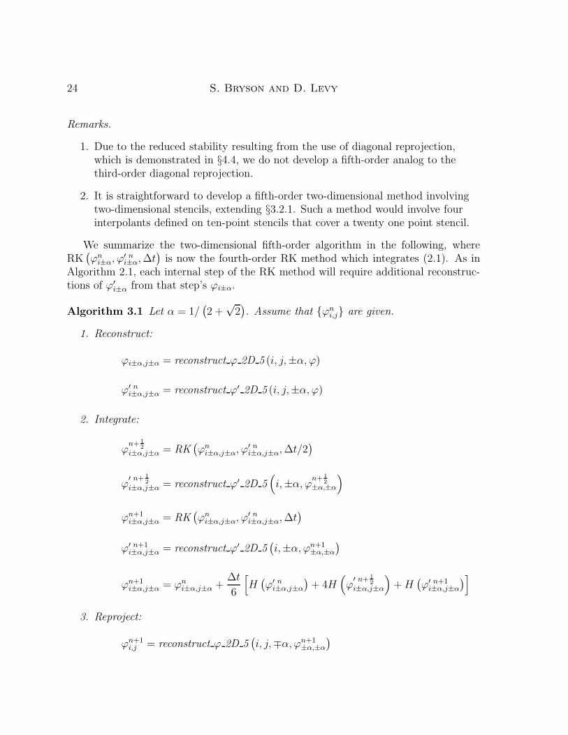
1. Due to the reduced stability resulting from the use of diagonal reprojection,which is demonstrated in §4.4, we do not develop a fifth-order analog to thethird-order diagonal reprojection.

2. It is straightforward to develop a fifth-order two-dimensional method involvingtwo-dimensional stencils, extending §3.2.1. Such a method would involve fourinterpolants defined on ten-point stencils that cover a twenty one point stencil.

We summarize the two-dimensional fifth-order algorithm in the following, whereRK

(

ϕni±α, ϕ′ n

i±α, ∆t)

is now the fourth-order RK method which integrates (2.1). As inAlgorithm 2.1, each internal step of the RK method will require additional reconstruc-tions of ϕ′i±α from that step’s ϕi±α.

Algorithm 3.1 Let α = 1/(

2 +√

2)

. Assume that {ϕni,j} are given.

1. Reconstruct:

ϕi±α,j±α = reconstruct ϕ 2D 5 (i, j,±α, ϕ)

ϕ′ ni±α,j±α = reconstruct ϕ′ 2D 5 (i, j,±α, ϕ)

2. Integrate:

ϕn+ 1

2

i±α,j±α = RK(

ϕni±α,j±α, ϕ′ n

i±α,j±α, ∆t/2)

ϕ′ n+ 1

2

i±α,j±α = reconstruct ϕ′ 2D 5(

i,±α, ϕn+ 1

2

±α,±α

)

ϕn+1i±α,j±α = RK

(

ϕni±α,j±α, ϕ′ n

i±α,j±α, ∆t)

ϕ′ n+1i±α,j±α = reconstruct ϕ′ 2D 5

(

i,±α, ϕn+1±α,±α

)

ϕn+1i±α,j±α = ϕn

i±α,j±α +∆t

6

[

H(

ϕ′ ni±α,j±α

)

+ 4H(

ϕ′ n+ 1

2

i±α,j±α

)

+ H(

ϕ′ n+1i±α,j±α

)

]

3. Reproject:

ϕn+1i,j = reconstruct ϕ 2D 5

(

i, j,∓α, ϕn+1±α,±α

)


3.4 Multi-Dimensional Extensions

The extension of the direction-by-direction approach to more than two space dimensionsis straightforward. For example, using the notation of §3.3, a three-dimensional fifth-order reconstruction is

1. For each i, j, k: ϕi+α,j,k = reconstruct ϕ 1D 5 (i, α, ϕ∗,j,k)

2. For each i, j, k: ϕi+α,j+α,k = reconstruct ϕ 1D 5 (j, α, ϕi+α,∗,k).

3. For each i, j, k: ϕi+α,j+α,k+α = reconstruct ϕ 1D 5 (k, α, ϕi+α,j+α,∗).

The reconstruction at xi−α,j−α,k−α is handled similarly, and the same for the reconstruc-tion of ϕ′i+α,j+α,k+α. In three dimensions α = 1/

(

3 +√

3)

.A d-dimensional reconstruction based on d-dimensional stencils quickly becomes very

large. It is readily apparent that the dimension-by-dimension approach will scale to highdimensions better than d-dimensional interpolants.

4 Numerical Simulations

In this section we present simulations that test the schemes we developed in this paper.In §4.1 we demonstrate the third- and fifth-order method in one dimension. §4.2 focuseson the fifth-order method in two and three space dimensions. In §4.3 we comparethe two-dimensional third-order method based on two-dimensional stencils with thedirection-by-direction approach. In §4.4 we examine, in detail, stability issues in twodimensions, including comparisons with [17]. Some of these examples are standard testcases that can be found, e.g., in [22, 31, 35].

We do not follow the practice in [17] of masking singular regions from our errormeasurements.

4.1 One-Dimensional Examples

A convex Hamiltonian

We start by testing the performance of our schemes on a convex Hamiltonian. Weapproximate solutions of the one-dimensional equation

φt +1

2(φx + 1)2 = 0, (4.1)

subject to the initial data φ(x, 0) = − cos(πx) with periodic boundary conditions on[0, 2]. The change of variables, u (x, t) = φx (x, t) + 1, transforms the equation intothe Burgers’ equation, ut + 1

2(u2)x = 0, which can be easily solved via the method of


characteristics [35]. As is well known, Burgers’ equation generally develops discontinuoussolutions even with smooth initial data, and hence we expect the solutions of (4.1) tohave discontinuous derivatives. In our case, the solution develops a singularity at timet = π−2.

The results of our simulations are shown in Figure 4.1. The order of accuracy ofthese methods is determined from the relative L1 error (see [30]), defined as the L1-normof the error divided by the L1-norm of the exact solution. These results along with therelative L∞-norm before the singularity, at T = 0.8/π2, are given in Table 4.1, and afterthe singularity at T = 1.5/π2 in Table 4.2.

Third-order method

N relative L1-error L1-order relative L∞-error L∞-order

100 9.41×10−5 – 1.77×10−5 –200 1.13×10−5 3.06 1.33×10−6 3.73400 1.39×10−6 3.02 9.35×10−8 3.83800 1.74×10−7 3.00 5.94×10−9 3.00

Fifth-order method


100 1.41×10−5 – 2.61×10−6 –200 4.21×10−7 5.07 4.03×10−8 6.02400 3.31×10−8 5.00 6.53×10−10 5.95800 4.03×10−10 5.03 1.00×10−11 6.03

Table 4.1: Relative L1-errors for the one-dimensional convex HJ problem (4.1) beforethe singularity formation. T = 0.8/π2.

A non-convex Hamiltonian

In this example we deal with non-convex Hamilton-Jacobi equations. In one dimensionwe solve

φt − cos (φx + 1) = 0, (4.2)

subject to the initial data φ (x, 0) = − cos (πx) with periodic boundary conditions on[0, 2]. In this case (4.2) has a smooth solution for t . 1.049/π2, after which a sin-gularity forms. A second singularity forms at t ≈ 1.29/π2. The results are shown inFigures 4.2. The convergence results before and after the singularity formation are givenin Tables 4.3–4.4.


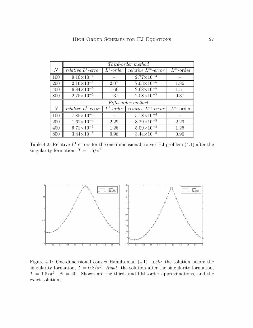
Third-order method


100 9.10×10−4 – 2.77×10−4 –200 2.16×10−4 2.07 7.63×10−5 1.86400 6.84×10−5 1.66 2.68×10−5 1.51800 2.75×10−5 1.31 2.08×10−5 0.37

Fifth-order method


100 7.85×10−4 – 5.78×10−4 –200 1.61×10−4 2.29 8.29×10−5 2.29400 6.71×10−5 1.26 5.09×10−5 1.26800 3.44×10−5 0.96 3.44×10−5 0.96

Table 4.2: Relative L1-errors for the one-dimensional convex HJ problem (4.1) after thesingularity formation. T = 1.5/π2.

0 0.2 0.4 0.6 0.8 1 1.2 1.4 1.6 1.8 2-1.5

-1

-0.5

0

0.5

1

exact 3rd-order fifth-order

0 0.2 0.4 0.6 0.8 1 1.2 1.4 1.6 1.8 2-1.2

-1

-0.8

-0.6

-0.4

-0.2

0

0.2

0.4

0.6

0.8


Figure 4.1: One-dimensional convex Hamiltonian (4.1). Left: the solution before thesingularity formation, T = 0.8/π2. Right: the solution after the singularity formation,T = 1.5/π2. N = 40. Shown are the third- and fifth-order approximations, and theexact solution.


Third-order method


100 6.47×10−5 – 9.05×10−6 –200 7.78×10−6 3.06 1.11×10−6 3.03400 8.77×10−7 3.15 9.27×10−8 3.58800 9.87×10−8 3.15 6.12×10−9 3.92

Fifth-order method


100 1.29×10−5 – 4.97×10−6 –200 6.52×10−7 4.31 2.38×10−7 4.38400 2.10×10−8 4.95 6.13×10−9 5.28800 5.96×10−10 5.14 1.03×10−10 5.90

Table 4.3: Relative L1-errors for the one-dimensional non-convex HJ problem (4.2)before the singularity formation. T = 0.8/π2.

Third-order method


100 2.81×10−4 – 9.64×10−5 –200 1.32×10−4 1.08 5.05×10−5 0.93400 2.31×10−5 2.52 6.00×10−6 3.07800 8.43×10−6 1.46 3.30×10−6 0.86

Fifth-order method


100 1.57×10−4 – 1.12×10−4 –200 8.34×10−5 0.91 6.60×10−5 0.77400 1.22×10−5 2.78 8.64×10−6 2.93800 6.67×10−5 0.87 5.23×10−6 .072

Table 4.4: Relative L1-errors for the one-dimensional non-convex HJ problem (4.2) afterthe singularity formation. T = 1.5/π2.


0 0.2 0.4 0.6 0.8 1 1.2 1.4 1.6 1.8 2-1

-0.5

0

0.5

1

1.5


0 0.2 0.4 0.6 0.8 1 1.2 1.4 1.6 1.8 2-1

-0.5

0

0.5

1

1.5


Figure 4.2: One-dimensional non-convex Hamiltonian (4.2). Left: The solution beforethe singularity formation, T = 0.8/π2. Right: The solution after the singularity forma-tion, T = 1.5/π2. N = 40. Shown are the third- and fifth-order approximations, andthe exact solution.

A linear advection equation

In this example ([17] with a misprint, corrected in [40]) we solve the one-dimensionallinear advection equation, i.e., H (φx) = φx. We assume periodic boundary conditionson [−1, 1], and take the initial data as φ (x, 0) = g (x− 0.5) on [−1, 1], where

g (x) = −(√

3

2+

9

2+

2π

3

)

(x + 1) + h(x),

h(x) =

2 cos(

3π2

x2)

−√

3, −1 < x < − 13,

3/2 + 3 cos (2πx) , − 13

< x < 0,15/2− 3 cos (2πx) , 0 < x < 1

3,

(28 + 4π + cos (3πx)) /3 + 6πx (x− 1) , 13

< x < 1.

(4.3)

The results of the fifth-order method are shown in Figure 4.3, where it is compared withthe fifth-order method of [17]. The reduced dissipation effects of our method are visiblein the reduced round-off of the corners.


-1 -0.5 0 0.5 1-6

-5

-4

-3

-2

-1t = 2

-1 -0.5 0 0.5 1-6

-5

-4

-3

-2

-1t = 8

-1 -0.5 0 0.5 1-6

-5

-4

-3

-2

-1t = 16

-1 -0.5 0 0.5 1-6

-5

-4

-3

-2

-1t = 32

exact fifth-order Jiang and Peng

Figure 4.3: One-dimensional linear advection, (4.3). T = 2, 8, 16, 32. N = 100. Crosses:our fifth-order method. Circles: the fifth-order method of [17] with a local Lax-Friedrichsflux. Solid line: the exact solution.


4.2 Two-Dimensional Examples

A convex Hamiltonian

In two dimensions we solve a problem similar to (4.1)

φt +1

2(φx + φy + 1)2 = 0, (4.4)

which can be reduced to a one-dimensional problem via the coordinate transformation(

ξη

)

= 12

(

1 11 −1

)(

xy

)

. The results of the fifth-order calculations for the initial

data φ (x, y, 0) = − cos (π(x + y)/2) = − cos (πξ) are shown in Figure 4.4. The conver-gence rates for the two-dimensional fifth-order scheme before and after the singularityare shown in Table 4.5.

Before singularity T = 0.8/π2


50 1.19×10−4 – 7.78×10−7 –100 6.80×10−6 4.13 1.64×10−8 5.56200 1.73×10−7 5.30 1.12×10−10 7.20

After singularity T = 1.5/π2


50 1.32×10−3 – 2.07×10−5 –100 3.89×10−4 1.76 3.60×10−6 2.52200 4.86×10−5 3.00 1.69×10−7 4.41

Table 4.5: Relative L1- and L∞-errors for the two-dimensional convex HJ problem (4.4)before and after singularity formation, computed via the fifth-order method.

A non-convex Hamiltonian

The two-dimensional non-convex problem, which is analogous to the one-dimensionalproblem, (4.2), is

φt − cos (φx + φy + 1) = 0. (4.5)

Here we assume initial data that is given by φ (x, y, 0) = − cos (π(x + y)/2), and periodicboundary conditions. The results are shown in Figure 4.5. The convergence results forthe two-dimensional fifth-order scheme before and after the singularity formation aregiven in Table 4.6.


-2

-1

0

1

2 -2-1.5

-1-0.5

00.5

11.5

2

-1.5

-1

-0.5

0

0.5

1

-2

-1

0

1

2 -2-1.5

-1-0.5

00.5

11.5

2

-1.5

-1

-0.5

0

0.5

1

Figure 4.4: Two-dimensional convex Hamiltonian, (4.4). Left: the solution before thesingularity formation, T = 0.8/π2. Right: the solution after the singularity formation,T = 1.5/π2. N = 40× 40. The solution is computed with the fifth-order method.



50 1.11×10−4 – 1.26×10−6 –100 6.91×10−6 4.00 2.42×10−8 5.70200 3.85×10−7 4.17 6.27×10−10 5.27



50 1.47×10−3 – 8.58×10−6 –100 1.93×10−4 2.93 9.27×10−7 3.21200 8.87×10−5 1.12 3.09×10−7 1.58

Table 4.6: Relative L1- and L∞-errors for the two-dimensional non-convex HJ problem(4.5) before and after the singularity formation, computed with the fifth-order method.


-2

-1

0

1

2 -2-1.5

-1-0.5

00.5

11.5

2

-1

-0.5

0

0.5

1

1.5

-2

-1

0

1

2 -2-1.5

-1-0.5

00.5

11.5

2

-1

-0.5

0

0.5

1

1.5

Figure 4.5: Two-dimensional non-convex Hamiltonian, (4.4). Left: the solution beforethe singularity formation, T = 0.8/π2. Right: the solution after the singularity for-mation, T = 1.5/π2. N = 40 × 40. The solution is computed with the fifth-ordermethod.

A fully two-dimensional example

The above two-dimensional examples are actually one-dimensional along the diagonal.To check the performance of our methods on fully two-dimensional problems we solve

φt + φxφy = 0, (4.6)

on [−π, π] × [−π, π], subject to the initial data φ (x, y, 0) = sin (x) + cos (y) with pe-riodic boundary conditions. The exact solution for this problem is given implicitly byφ (x, y, t) = − cos (q) sin (r)+sin (q)+cos (r) where x = q− t sin (r) and y = r+ t cos (q).This solution is smooth for t < 1, continuous for all t and has discontinuous derivativesfor t ≥ 1. The results of our simulations at times T = 0.8, 1.5, are shown in Figure 4.6.The convergence results for the fifth-order two-dimensional schemes before the singular-ity formation are given in Table 4.7 and confirm the expected order of accuracy of ourmethods.

An eikonal equation in geometric optics

We consider a two-dimensional non-convex problem that arises in geometric optics [20]{

φt +√

φ2x + φ2

y + 1 = 0,φ (x, y, 0) = 1

4(cos (2πx)− 1) (cos (2πy)− 1)− 1.

(4.7)


Before singularity T = 0.8N relative L1-error L1-order relative L∞-error L∞-order

50 6.10×10−6 – 8.15×10−8 –100 2.10×10−7 4.86 7.35×10−10 6.79200 7.53×10−9 4.80 5.59×10−12 7.04

Table 4.7: Relative L1-errors for the two-dimensional HJ problem (4.6) before singularityformation. T = 0.8. The solution is computed with the fifth-order method.

-4

-2

0

2

4 -4

-3

-2

-1

0

1

2

3

4-2

-1

0

1

2

-4

-2

0

2

4 -4

-3

-2

-1

0

1

2

3

4-2

-1

0

1

2

Figure 4.6: Fully two-dimensional Hamiltonian, (4.6). Left: the solution before thesingularity formation, T = 0.8. Right: the solution after the singularity formation,T = 1.5. N = 50× 50. The solution is computed with the fifth-order method.


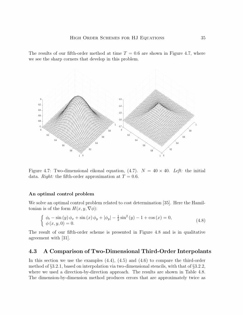
The results of our fifth-order method at time T = 0.6 are shown in Figure 4.7, wherewe see the sharp corners that develop in this problem.

0

0.2

0.4

0.6

0.8

1 0

0.2

0.4

0.6

0.8

1-1

-0.8

-0.6

-0.4

-0.2

0

0

0.2

0.4

0.6

0.8

1 0

0.2

0.4

0.6

0.8

1-1.7

-1.6

-1.5

-1.4

-1.3

Figure 4.7: Two-dimensional eikonal equation, (4.7). N = 40 × 40. Left: the initialdata. Right: the fifth-order approximation at T = 0.6.

An optimal control problem

We solve an optimal control problem related to cost determination [35]. Here the Hamil-tonian is of the form H(x, y,∇φ):

{

φt − sin (y)φx + sin (x) φy + |φy| − 12sin2 (y)− 1 + cos (x) = 0,

φ (x, y, 0) = 0.(4.8)

The result of our fifth-order scheme is presented in Figure 4.8 and is in qualitativeagreement with [31].

4.3 A Comparison of Two-Dimensional Third-Order Interpolants

In this section we use the examples (4.4), (4.5) and (4.6) to compare the third-ordermethod of §3.2.1, based on interpolation via two-dimensional stencils, with that of §3.2.2,where we used a direction-by-direction approach. The results are shown in Table 4.8.The dimension-by-dimension method produces errors that are approximately twice as


-4

-2

0

2

4 -4

-3

-2

-1

0

1

2

3

4-1

0

1

2

3

Figure 4.8: Two-dimensional optimal control problem, (4.8). An approximation withthe fifth-order method is shown at T = 1. N = 40× 40.

large compared with the genuinely two-dimensional reconstrcution. However, the con-vergence rate is qualitatively the same in both methods. These results motivated us tobase our fifth-order scheme on the much simpler dimension-by-dimension reconstruction.

4.4 A Stability Study

In this section we present a couple of stability studies we obtained in our simulations.We start by checking the stability properties of the third-order scheme with differentreprojection steps. The reconstruction step is done in all cases using the direction-by-direction interpolant. We compare the dimension-by-dimension reprojection and thediagonal reprojection (of §3.2.3). In Figure 4.9 we plot the L1 error as a function of theCFL number. The test problem is (4.6) with the fully two-dimensional Hamiltonian.The solution is computed at T = 0.8. We see that the use of a diagonal reprojectionsignificantly reduces the maximum allowed CFL number.

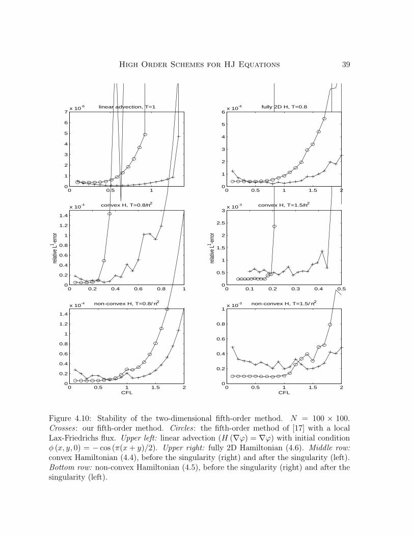
We now turn to checking the stability properties of the two-dimensional fifth-ordermethod of §3.3 by computing the L1 errors for various examples while varying the CFLnumber. In Figure 4.10 we compare the results obtained with our fifth-order schemewith the fifth-order method of [17], for which we used a local Lax-Friedrichs flux. Thenumerical tests indicate that larger CFL numbers can be used with our method.


2D Stencils Direction-by-Direction

N relative L1-error L1-order relative L1-error L1-order

Convex Hamiltonian at T = 0.8/π2

50 4.70×10−4 – 6.13×10−4 –100 7.54×10−5 2.64 9.43×10−5 2.70200 8.07×10−6 3.23 1.02×10−5 3.21

Convex Hamiltonian at T = 1.5/π2

50 1.23×10−3 – 2.61×10−3 –100 4.56×10−4 1.44 8.19×10−4 1.67200 3.70×10−5 3.62 1.22×10−4 2.74

Non-Convex Hamiltonian at T = 0.8/π2

50 2.27×10−4 – 3.92×10−4 –100 3.75×10−5 2.60 6.97×10−5 2.49200 3.99×10−6 3.23 7.22×10−6 3.27

Non-Convex Hamiltonian at T = 1.5/π2

50 1.23×10−3 – 1.94×10−3 –100 2.50×10−4 2.30 4.16×10−4 2.22200 7.63×10−5 1.71 1.20×10−4 1.79

Fully 2D Example at T = 0.850 2.01×10−4 – 1.48×10−4 –100 2.42×10−5 3.05 1.65×10−5 3.16200 2.95×10−6 3.04 1.95×10−6 3.08

Table 4.8: Comparison of the third-order method of §3.2.1, with an interpolation viatwo-dimensional stencils, and that of §3.2.2, with the direction-by-direction approach.


1.5 1.6 1.7 1.8 1.9 2 2.1 2.2 2.3 2.4 2.50

0.1

0.2

0.3

0.4

0.5

0.6

0.7

0.8

0.9

1x 10

-4 Third order fully 2D H, T=0.8

CFL

rela

tive

L1 -err

or

Figure 4.9: Stability of the two-dimensional third-order method with a dimension-by-dimension (crosses) vs. a diagonal reprojection (diamonds). Fully two-dimensionalHamiltonian (4.6). T = 0.8 (before singularity). N = 100× 100.


0 0.5 10

1

2

3

4

5

6

7x 10

-6 linear advection, T=1

0 0.2 0.4 0.6 0.8 10

0.2

0.4

0.6

0.8

1

1.2

1.4

x 10-4 convex H, T=0.8/π2

relat

ive L

1 -erro

r

0 0.1 0.2 0.3 0.4 0.50

0.5

1

1.5

2

2.5

3x 10

-3 convex H, T=1.5/π2

relat

ive L

1 -erro

r

0 0.5 1 1.5 20

0.2

0.4

0.6

0.8

1

1.2

1.4

x 10-4 non-convex H, T=0.8/π2

CFL0 0.5 1 1.5 2

0

0.2

0.4

0.6

0.8

1x 10

-3 non-convex H, T=1.5/π2

CFL

0 0.5 1 1.5 20

1

2

3

4

5

6x 10

-6 fully 2D H, T=0.8

Figure 4.10: Stability of the two-dimensional fifth-order method. N = 100 × 100.Crosses: our fifth-order method. Circles: the fifth-order method of [17] with a localLax-Friedrichs flux. Upper left: linear advection (H (∇ϕ) = ∇ϕ) with initial conditionφ (x, y, 0) = − cos (π(x + y)/2). Upper right: fully 2D Hamiltonian (4.6). Middle row:

convex Hamiltonian (4.4), before the singularity (right) and after the singularity (left).Bottom row: non-convex Hamiltonian (4.5), before the singularity (right) and after thesingularity (left).


4.5 Three-Dimensional Examples

We proceed with a three-dimensional generalization of the convex Hamiltonian (4.4),

φt +1

2(φx + φy + φz + 1)2 = 0, (4.9)

subject to the initial data φ (x, y, z, 0) = − cos (π(x + y + z)/3). The convergence resultsfor the three-dimensional fifth-order scheme before and after the singularity formationare given in Table 4.9. We also approximate the solution of the non-covex problem

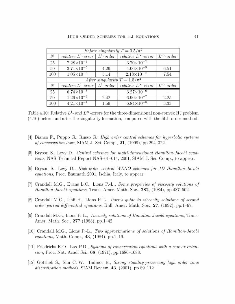
φt − cos (φx + φy + φz + 1) = 0, (4.10)

with the same initial data. The convergence rates for the three-dimensional fifth-orderschemes are given in Table 4.10.



25 2.61×10−4 – 1.07×10−7 –50 6.40×10−6 5.35 3.16×10−10 8.41100 1.50×10−7 5.42 9.18×10−13 8.43



25 6.95×10−3 – 1.80×10−5 –50 1.40×10−3 2.31 4.15×10−6 2.12100 5.33×10−4 1.39 6.94×10−7 2.58

Table 4.9: Relative L1- and L∞-errors for the three-dimensional convex HJ problem(4.9) before and after the singularity formation, computed with the fifth-order method.

References

[1] Abgrall R., Numerical discretization of the first-order Hamilton-Jacobi equation on

triangular meshes, Comm. Pure Appl. Math., 49, (1996), pp.1339–1373.

[2] Arminjon P., Viallon M.-C., Generalisation du schema de Nessyahu-Tadmor pour

une equation hyperbolique a deux dimensions d’espace, C.R. Acad. Sci. Paris, t.320, serie I. (1995), pp.85–88.

[3] Barles G., Solution de viscosite des equations de Hamilton-Jacobi, Springer-Verlag,Berlin, 1994.




25 7.28×10−4 – 3.70×10−7 –50 3.71×10−5 4.29 4.06×10−9 6.51100 1.05×10−6 5.14 2.18×10−11 7.54



25 6.74×10−3 – 3.27×10−6 –50 1.26×10−3 2.42 6.90×10−7 2.25100 4.21×10−4 1.59 6.84×10−8 3.33

Table 4.10: Relative L1- and L∞-errors for the three-dimensional non-convex HJ problem(4.10) before and after the singularity formation, computed with the fifth-order method.

[4] Bianco F., Puppo G., Russo G., High order central schemes for hyperbolic systems

of conservation laws, SIAM J. Sci. Comp., 21, (1999), pp.294–322.

[5] Bryson S., Levy D., Central schemes for multi-dimensional Hamilton-Jacobi equa-

tions, NAS Technical Report NAS–01–014, 2001, SIAM J. Sci. Comp., to appear.

[6] Bryson S., Levy D., High-order central WENO schemes for 1D Hamilton-Jacobi

equations, Proc. Enumath 2001, Ischia, Italy, to appear.

[7] Crandall M.G., Evans L.C., Lions P.-L., Some properties of viscosity solutions of

Hamilton-Jacobi equations, Trans. Amer. Math. Soc., 282, (1984), pp.487–502.

[8] Crandall M.G., Ishii H., Lions P.-L., User’s guide to viscosity solutions of second

order partial differential equations, Bull. Amer. Math. Soc., 27, (1992), pp.1–67.

[9] Crandall M.G., Lions P.-L., Viscosity solutions of Hamilton-Jacobi equations, Trans.Amer. Math. Soc., 277 (1983), pp.1–42.

[10] Crandall M.G., Lions P.-L., Two approximations of solutions of Hamilton-Jacobi

equations, Math. Comp., 43, (1984), pp.1–19.

[11] Friedrichs K.O., Lax P.D., Systems of conservation equations with a convex exten-

sion, Proc. Nat. Acad. Sci., 68, (1971), pp.1686–1688.

[12] Gottlieb S., Shu C.-W., Tadmor E., Strong stability-preserving high order time

discretization methods, SIAM Review, 43, (2001), pp.89–112.


[13] Harten A., Engquist B., Osher S., Chakravarthy S., Uniformly high order accurate

essentially non-oscillatory schemes III, J. Comput. Phys., 71, (1987), pp.231–303.

[14] Hu C., Shu C.-W., A discontinuous Galerkin finite element method for Hamilton-

Jacobi equations, SIAM J. Sci. Comp., 21, (1999), pp.666–690.

[15] Kruzkov S.N., The Cauchy problem in the large for nonlinear equations and for

certain quasilinear systems of the first order with several variables, Soviet Math.Dokl., 5, (1964), pp.493–496.

[16] Jiang G.-S., Levy D., Lin C.-T., Osher S., Tadmor E., High-resolution non-

oscillatory central schemes with non-staggered grids for hyperbolic conservation laws,SIAM J. Num. Anal., 35, (1998), pp.2147–2168.

[17] Jiang G.-S., Peng D., Weighted ENO schemes for Hamilton-Jacobi equations, SIAMJ. Sci. Comp., 21, (2000), pp.2126–2143.

[18] Jiang G.-S., Shu C.-W., Efficient implementation of weighted ENO schemes, JCP,126, (1996), pp.202–228.

[19] Jiang G.-S., Tadmor E., Nonoscillatory central schemes for multidimensional hy-

perbolic conservation laws, SIAM J. Sci. Comp., 19, (1998), pp.1892–1917.

[20] Jin S., Xin Z., Numerical passage from systems of conservation laws to Hamilton-

Jacobi equations and relaxation schemes, SIAM J. Numer. Anal., 35, (1998),pp.2385–2404.

[21] Kurganov A., Noelle S., Petrova G., Semi-discrete central-upwind schemes for hy-

perbolic conservation laws and Hamilton-Jacobi equations, SIAM J. Sci. Comp., 23,(2001), pp.707–740.

[22] Kurganov A., Tadmor E., New high-resolution semi-discrete central schemes for

Hamilton-Jacobi equations, JCP, 160, (2000), pp.720–724.

[23] Kurganov A., Tadmor E., New high-resolution central schemes for nonlinear con-

servation laws and convection-diffusion equations, JCP, 160, (2000), pp.241–282.

[24] Lepsky O., Hu C., Shu C.-W., Analysis of the discontinuous Galerkin method for

Hamilton-Jacobi equations, Appl. Numer. Math., 33, (2000), pp.423–434.

[25] Levy D., Puppo G., Russo G., A fourth order central WENO scheme for multi-

dimensional hyperbolic systems of conservation laws, SIAM J. Sci. Comp., to appear.


[26] Levy D., Puppo G., Russo G., Central WENO schemes for hyperbolic systems of

conservation laws, Math. Model. and Numer. Anal., 33, no. 3 (1999), pp.547–571.

[27] Levy D., Puppo G., Russo G., Compact central WENO schemes for multidimen-

sional conservation laws, SIAM J. Sci. Comp., 22, (2000), pp.656–672.

[28] Lions P.L., Generalized solutions of Hamilton-Jacobi equations, Pitman, London,1982.

[29] Lions P.L., Souganidis P.E., Convergence of MUSCL and filtered schemes for

scalar conservation laws and Hamilton-Jacobi equations, Numer. Math., 69, (1995),pp.441–470.

[30] Lin C.-T., Tadmor E., L1-stability and error estimates for approximate Hamilton-

Jacobi solutions, Numer. Math., 87, (2001), pp.701–735.

[31] Lin C.-T., Tadmor E., High-resolution non-oscillatory central schemes for approx-

imate Hamilton-Jacobi equations, SIAM J. Sci. Comp., 21, no. 6, (2000), pp.2163–2186.

[32] Liu X.-D., Osher S., Chan T., Weighted essentially non-oscillatory schemes, JCP,115, (1994), pp.200–212.

[33] Nessyahu H., Tadmor E., Non-oscillatory central differencing for hyperbolic conser-

vation laws, JCP, 87, no. 2 (1990), pp.408–463.

[34] Osher S., Sethian J., Fronts propagating with curvature dependent speed: algorithms

based on Hamilton-Jacobi formulations, JCP, 79, (1988), pp.12–49.

[35] Osher S., Shu C.-W., High-order essentially nonoscillatory schemes for Hamilton-

Jacobi equations, SIAM J. Numer. Anal., 28, (1991), pp.907–922.

[36] Shi J., Hu C., Shu C.-W., A technique of treating negative weights in WENO

schemes, JCP, to appear.

[37] Shu C.-W., Osher S., Efficient implementation of essentially non-oscillatory shock-

capturing schemes, II, JCP, 83, (1989), pp.32–78.

[38] Souganidis P.E., Approximation schemes for viscosity solutions of Hamilton-Jacobi

equations, J. Diff. Equations., 59, (1985), pp.1–43.

[39] Zennaro M., Natural continuous extensions of Runge-Kutta methods, Math. Comp.,46, (1986), pp.119–133.


[40] Zhang Y.-T., Shu C.-W., High-order WENO schemes for Hamilton-Jacobi equations

on triangular meshes, NASA/CR–2001–211256, ICASE Report No. 2001–39, (2001),submitted to SIAM J. Numer. Anal.

high-order central weno schemes for multi-dimensional ... · pdf filehigh-order central weno...

Documents