multi-domain hybrid spectral-weno methods for …bcosta/papers/hybrid1d.pdf · multi-domain hybrid...

Multi-Domain Hybrid Spectral-WENO Methods for Hyperbolic

Conservation Laws

Bruno Costa ∗ Wai Sun Don †

February 15, 2006

Abstract

In this article we introduce the multi-domain hybrid Spectral-WENO method aimed at the discon-tinuous solutions of hyperbolic conservation laws. The main idea is to conjugate the non-oscillatoryproperties of the high order weighted essentially non-oscillatory (WENO) finite difference schemes withthe high computational efficiency and accuracy of spectral methods. Built in a multi-domain framework,subdomain adaptivity in space and time is used in order to maintain the solutions parts exhibiting highgradients and discontinuities always inside WENO subdomains while the smooth parts of the solutionare kept in spectral ones. A high order multi-resolution algorithm by Ami Harten [6]is used to deter-mine the smoothness of the solution in each subdomain. Numerical experiments with the simulation ofcompressible flow in the presence of shock waves are performed.

KeywordsSpectral, WENO, Multi-resolution, Multi-Domain, Hybrid, Conservation Laws

AMS65P30, 77Axx

1 Introduction

The fine scale and delicate structures of physical phenomena related to turbulence demand the utilizationof high order methods when performing numerical simulations. Spectral methods nondispersiveness andnondissipativity make them well fitted to this task when the solutions involved are smooth. However, inthe modeling of compressible turbulent flows by means of the inviscid Euler Equations, the development offinite time discontinuities generates global O(1) oscillations, known as the Gibbs phenomenon, causing lossof accuracy and numerical instability. Filtering of small scales has been used to stabilize the spectral schemein shock calculations [13], however the Gibbs oscillations still remain in the solution.See Figure 1, where the density of the Lax shock tube problem with Riemann initial conditions was obtainedwith a Chebyshev collocation method and a 16 th order exponential filter. Note that the oscillations alsooccur at a smaller scale on the edges of the rarefaction wave, due to the discontinuities at the derivativeof the density. The use of heavy filtering is not recommended as it would remove the fine scale physicalstructures which are important for the overall fidelity of the simulations.Reconstruction techniques such as the direct and inverse Gegenbauer expansions (see [4, 28] and referencescontained therein) have achieved some success as a postprocessing treatment to remove the Gibbs oscilla-tions. These techniques followed the achievement of relevant theoretical results demonstrating convergenceproperties of spectral approximations of discontinuous solutions. For instance, Gottlieb and Tadmor [5]proved that, for linear problems, the moments of the numerical solution computed by spectral methods arespectrally accurate. Lax [8] had argued that high order information about the solution is contained in high

∗Departamento de Matematica Aplicada, IM-UFRJ, Caixa Postal 68530, Rio de Janeiro, RJ, C.E.P. 21945-970, Brazil.E-Mail: [email protected]

†Division of Applied Mathematics, Brown University, Providence, Rhode Island 02912.E-Mail: [email protected]

1

HYBRID SPECTRAL-WENO METHODS FOR CONSERVATION LAWS 2

x

Rh

o

4 2 0 2 40

0.2

0.4

0.6

0.8

1

1.2

1.4

x

Rh

o

4 2 0 2 40

0.2

0.4

0.6

0.8

1

1.2

1.4

Figure 1: The density of the Lax problem as computed by (Left) the Chebyshev collocation solution withthe Gibbs oscillations and (Right) the fifth-order characteristic-wise WENO finite difference scheme. Theexact solution is represented by the solid line.

resolution schemes, even for nonlinear problems. Hence highly accurate essentially non-oscillatory solutioncan be extracted from the seemingly oscillatory noisy data. Tadmor [10] showed the convergence of spectralmethods for nonlinear scalar equations. Nevertheless, the rapid growth rate of the Gegenbauer polynomialscause several numerical problems which are difficult to overcome. Very often, the domain must be subdividedin order to apply the Gegenbauer reconstruction when dealing with complex and localized flow structures.The numerical difficulties associated with the global spectral methods are some of the main reasons whylocal nonlinear adaptive shock capturing finite differences have been the method of choice when dealingwith nonlinear conservation laws. Among these, the most commonly used is the Essentially Non-Oscillatoryschemes (ENO) [21]. In order to avoid numerical oscillations, ENO schemes bias the local stencil, discardinginterpolations across the discontinuities when computing the tendencies of the numerical solution. TheWeighted Essentially non-Oscillatory (WENO) method (see [23]) is an improvement over the ENO methodwith the introduction of an adaptive choice for the reconstruction stencils. WENO achieves optimal orderof accuracy at smooth parts of the solution with the same stencil size of ENO. Nevertheless, the intrinsicnumerical dissipation of WENO schemes, although necessary to properly capture shock waves, eventuallydamp the relevant small scales. Figure 1 also shows a solution of the same Lax problem obtained with afifth order characteristic-wise WENO finite difference scheme. Note the smearing of the shock, the contactinterface and of the edges of the rarefaction wave. The Numerical dissipation can be reduced by increasingthe number of points, as well as the order of the WENO scheme which, however, would make the schemeexpensive to apply. This would also means waste of computational effort since it would not change thesituation of well resolved structures at the smooth regions of the solution. Moreover, the fixed order of thefinite differences do not provide the exponential resolution of spectral schemes.This article aims at the conjugation of the spectral and WENO methods when solving hyperbolic equa-tions with discontinuous solutions. The general idea is to build a multi-domain scheme, forming a globaladaptive mesh composed of WENO and spectral subdomains in a way that discontinuities of the solutionare always contained within WENO subdomains and the smooth components remain in spectral ones. Asmoothness measurement device triggers the switching of the subdomains from spectral to WENO and re-ciprocally, according to the local behavior of the solution. For instance, the algorithm takes care of movingdiscontinuities by changing the spectral subdomains in their way to WENO ones and switching WENO sub-domains in their trails to spectral subdomains, guaranteeing higher numerical efficiency than the classicalsingle-domain WENO method and non-oscillatory solutions when compared with the classical single-domainspectral method. Moreover, the application of the spectral methods at smooth regions avoids the heavy ma-chinery employed by the characteristic-wise WENO finite difference algorithm such as the evaluation of theJacobian of the fluxes, the global Lax-Friedrichs flux splitting and the forward and backward characteristics


projections.The multi-domain hybrid Spectral-WENO method (Hybrid) here proposed can also be thought of as animprovement to the classical spectral method by using the ”WENO technique” to approximate disconti-nuities, in the same way that physical filtering is used. Based on the multi-domain framework, the Gibbsphenomenon is effectively avoided, since there will be no spectral approximation of discontinuities, whichalso discards the need of any postprocessing technique.This paper is organized as follows: Approximation theory of Spectral methods is briefly discussed in Section2. In Section 3, WENO Finite Differences schemes are described and Harten’s multi-resolution algorithm ispresented in Section 4. The Hybrid method along with its interfaces treatment and subdomain switchingprocedure are introduced in Section 5. Finally, in Section 6, we apply the Hybrid method to the standardshock-tube problems with Riemann data and to the Shock-Entropy wave interaction and the Blastwaveproblems.

2 Spectral Methods

We start this section with a quick description of Galerkin and Pseudospectral spectral methods, which intheir simplest forms, make use of a global smooth basis {φk(x), k = 0, . . . , N} to represent the numericalsolution. After that, we discuss the Gibbs Phenomenon for piecewise smooth functions and the utilizationof filtering to stabilize the spectral discretization of hyperbolic conservation laws.

2.1 Gibbs Phenomenon and Filtering for Spectral Methods

In the Galerkin approach, the function f(x) is projected into the set of basis function φk(x) as

PNf(x) =N∑

k=0

akφk(x), (1)

where PN is the projection operator. The coefficients ak are

ak =∫

f(x)φk(x)w(x)dx, (2)

with the appropriate weight function w(x) that depends on the nature of the physical solution:

• For periodic problems, the natural basis functions are the trigonometric polynomials of degree k, φk(x) =eiπkx with weight function w(x) = 1 and x ∈ [−1, 1).

• For non-periodic problems in a finite domain x ∈ [−1, 1], Chebyshev polynomials φk(x) = Tk(x) withw(x) = (1 − x2)−

12 or, Legendre polynomials φk(x) = Tk(x) with w(x) = 1 are the most used bases.

The Pseudospectral (Collocation) version of spectral methods approximates a function f(x) by an interpo-lating polynomial given by

INf(x) =N∑

k=0

akφk(x), ak =N∑

i=0

ωif(xi)φk(xi), (3)

where IN is the interpolation operator, xi and ωi are the Gauss-Lobatto quadrature nodes and weightsrespectively (Gauss-Radau and Gauss nodes can also be used). Alternatively,

INf(x) =N∑

j=0

f(xj )gj(x), (4)

where gj(x) are the cardinal functions: (trigonometric) Lagrangian interpolation polynomials of degree Nsuch that gj(xi) = δij . For the Lagrangian interpolation polynomials based on the Chebyshev Gauss-Lobattopoints xi = cos(πi/N ), i = 0, . . . , N , the cardinal functions are given by

gj(x) =(−1)j+1(1 − x2)T ′

N (x)cjN2(x − xj)

, (5)


where c0 = cN = 2, cj = 1, j = 1, . . . , N − 1 and TN (x) is the N th degree Chebyshev polynomial of the firstkind. The derivatives of f(x) at the collocation points xi can be computed via equations (3) or (4). Theformer makes use of the fast cosine transform (CFT) algorithm and the latter uses a matrix-vector algorithm.More details can be found in [1].

2.2 Conservation Laws: Gibbs Phenomenon and Filtering

The approximation error in spectral methods depends only on the regularity of the approximated function.A typical error estimate is of the form

|f(x) − PNf(x)| ≤ CN12−p

(∫ 2π

0

|f (p)(ξ)|2dξ

) 12

, (6)

where C is a constant independent of N and f (p) denotes the p th derivative of f . We see that the approxi-mation error decays as O(N−p) for any Cp function and if the function is analytic then

|f(x) − PNf(x)| ≤ Ce−αN , (7)

for some α > 0, resulting in exponential convergence. Similar results hold for the pseudospectral (collocation)formulation. However, in the case of piecewise smooth functions, the order of accuracy is reduced to O(1)due to the well known Gibbs phenomenon.Figure 2 below shows Fourier collocation approximations to a piecewise linear function with a discontinuityat x = 0. Note that the over- and under-shoot oscillations do not decrease with the increasing number ofgrid points N .

−4 −3 −2 −1 0 1 2 3 4−4

−3

−2

−1

0

1

2

3

4

N=32 N=16

N=8

Figure 2: Gibbs phenomenon in the spectral approximation of a sawtooth function.

Other important features of spectral methods are their inherent non-dissipativity and non-dispersiveness,which are good properties when important conservation principles need to be respected at the numericallevel. This lack of dissipation, however, becomes an issue when dealing with discontinuous solutions ofconservation laws, in particular, when spectral methods are applied to nonlinear hyperbolic equations in theconservation form and the problem of an entropy satisfying solution arises. In fact, there is no artificialdissipation in spectral methods to indicate that their solutions are limits of a dissipative process. Thisproblem had been addressed in [11] and the references contained therein, where it has been showed that witha suitable addition of a spectrally small dissipation to the high modes, the method is stable and entropicsolutions are obtained.The utilization of low pass filtering in spectral methods helps both to mitigate the Gibbs Phenomenon and tointroduce the necessary artificial dissipation for hyperbolic problems. Considering the Fourier approximation(The process is analogous for the Chebyshev case):

fN (x) =N∑

k=−N

akeiπkx, x ∈ [−1, 1), (8)


filtering is introduced by means of the modified sum

fσN (x) =

N∑

k=−N

σ

(k

N

)akeiπkx , (9)

where, following Vandeven [12], σ(ω) is a p th order, p > 1, Cp[−1, 1], filter function satisfying

σ(0) = 1 , σ(±1) = 0 ,

σ(j)(0) = 0 , σ(j)(±1) = 0 , j ≤ p,(10)

where σ(j) denotes its j th derivative.It has been shown in [12] that the filtered sum (9) approximates a discontinuous function in smooth regionswith exponential accuracy.In this work we make use of the exponential filter function

σ(ω) = exp(−α|ω|β

), (11)

where −1 ≤ ω = k/N ≤ 1, |k| = 0, . . . , N and β is the order of the filter. In order to satisfy numerically thefirst condition of (10) we set α = − ln ε, where ε is the machine zero.In Figure 3 the solution of the periodical inviscid Burgers equation is obtained with a Fourier collocationmethod with an 16 th order exponential filter.

x0 1 2 3 4 5 6

1.5

1

0.5

0

0.5

1

1.5

UN

x

Err

or

0 1 2 3 4 5 614

12

10

8

6

4

2

0

N=128

N=256

N=512

Figure 3: Fourier spectral solution of the Burgers equation with a 16 th order exponential filter. (Left)Filtered solution with 128 points. (Right) Convergence of the solution with N = 128, 256, 512. The error isin the log10 scale.

It is worth saying that no amount of filtering other than a heavy one (p ≤ 2), can remove the Gibbsoscillations from the solution. The use of such a filter, however, also incurs in removal of small and medianscale structures rendering the solution unusable and inaccurate.In practice, when solving differential equations one uses a high order exponential filter at every time step tomaintain stability and a post-processing technique [4, 28, 26] at the end of the calculation to recover a non-oscillatory solution from the oscillatory one. These post-processing techniques, however, are not practical,particularly, for multi-dimensional problems. As it is evident from Figure 3, in order to recover the fullaccuracy in any region where the function is continuous, one has to use a different idea. In the next sectionwe introduce essentially non-oscillatory finite differences schemes as the next step to build the hybrid scheme,where the ENO schemes will be applied to the discontinuous parts of the solution.


3 Weighted essentially non-oscillatory schemes

In this section we describe essentially non-oscillatory conservative finite difference schemes to be applied atsystems of conservation laws described by the general equation:

ut + f(u)x = 0. (12)

Being conservative is an important property of a numerical approximation due to the Lax–Wendroff theoremwhich states that if there is convergence of numerical solutions of conservative schemes, then they willconverge to a weak solution of the conservation law [8]. In this section, we will first present a general highorder conservative central scheme approximation to (12). After that, we will describe the adaptive stencilchoosing process that leads to the non-oscillatory properties of ENO and WENO schemes.A conservative finite-difference formulation for hyperbolic conservation laws requires high-order consistentnumerical fluxes at the cell boundaries in order to form the flux difference across the uniformly-spaced cells.Consider an uniform grid defined by the points xi = i∆x, for i = 0, . . . , N , which are also called cell centers,with cell boundaries given by xi+ 1

2= xi ± ∆x

2 . We semi-disctretize Equation (12) by the method of lines,yielding the following system of ordinary differential equations

dui(t)dt

= −∂f

∂x

∣∣∣∣x=xi

, i = 0, . . . , N (13)

where ui(t) is a numerical approximation to the cell center value u(xi, t).The conservative property of the spatial discretization is obtained by implicitly defining a numerical fluxfunction h(x) as

f(x) =1

∆x

∫ x+ ∆x2

x−∆x2

h(ξ)dξ, (14)

such that the spatial derivative in (13) is exactly approximated by a conservative finite difference formula atthe cell boundaries,

dui(t)dt

=1

∆x

(hi+ 1

2− hi− 1

2

), (15)

where hi± 12

= h(x ± ∆x2

). High order polynomial interpolations to hi± 12

are computed using known gridvalues of f .Note that the order of the polynomial interpolation of hi±1

2will set the order of the spatial approximation

of the overall scheme (15). Due to the symmetry of the stencils used for the polynomial interpolations, theorder of approximation of the right-hand side of (15) will be the same order of the polynomial approximationof h(x), even after division by ∆x, and not, as expected, one order less.Let us now solve the problem of finding a k th order central polynomial approximation to hi+ 1

2. Let

h(x) = a0 + a1x + · · ·+ ak−1xk−1 (16)

be a (k − 1) th degree polynomial approximation to h(x) and f (x) be the polynomial (also of degree k − 1)obtained by integration of (14) after the substitution of h(x) by h(x). The polynomial coefficients are foundafter evaluating f (x) at the grid points of any k nodes stencil around xi+ 1

2. For instance, if k = 3, the

coefficients a0, a1, a2 can be obtained as functions of the grid point values fi−1, fi and fi+1. Once thecoefficients are found, the values fi± 1

2= hi± 1

2+ O(∆xk) can be computed and substituted at (15).

The scheme above is centralized at xi+ 12

only if k is even, otherwise, it is shifted a half-cell to the left(upstream) or to the right (downstream). One often takes the upstream version of an odd order centralscheme due to the inherent dissipation of upstream schemes, necessary to shock-capturing. For the sakeof completeness, let us now take the case k = 5 and make the computations to obtain the 5 th orderapproximation to the spatial derivative in (15).Thus, after substitution of 4 th order polynomial in (14) and integration, we obtain

f (x) = a0 + a1x + a2

(x2 +

∆x2

2

)+ a3

(x3 +

x∆x2

4

)+ a4

(x4 +

x2∆x2

2

), (17)


which, if computed at the nodes {xi−2, . . . , xi+2} will determine the coefficients {a0, . . . , a4} in terms of{fi−2, . . . , fi+2}, yielding

fi+ 12

=160

(2fi−2 − 13fi−1 + 47fi + 27fi+1 − 3fi+2) , (18)

and, analogously,

fi− 12

=160

(2fi−3 − 13fi−2 + 47fi−1 + 27fi − 3fi+1) . (19)

Both are 5 th order approximations to hi+ 12

and hi−12, respectively:

fi± 12

= hi± 12− 1

60d5f

dx5

∣∣∣∣x=xi

+ O(∆x6). (20)

The leading error order is the same for both stencils, so they will cancel out after substitution of (18) and(19) at (15), yielding a 5 th order approximation as pointed out beforehand.The central finite difference scheme presented above will suffer from spurious oscillations if discontinuities areinside the interpolating stencils. The main idea of ENO schemes is to bias as much as necessary the centralscheme to avoid the inclusion of the shock inside the stencil. For instance, a k-th order ENO approximationassignes smoothness weights to all k nodes stencils around the interpolating point and chooses the smoothestone to perform k th order polynomial interpolations of the numerical flux.Let us identify a particular stencil by its left-shift r. We have a polynomial interpolation to hi+ 1

2for each r,

given by

fr(xi+ 12) =

k−1∑

j=0

crjfi−r+j = h(xi+ 12) + O(∆xk), (21)

where the crj are the Lagrangian interpolation coefficients (see [23]). The crj depend on the order k of theapproximation and also on the left-shift parameter r, but not on the values fi. Since r can vary from 0 to k−1,we have k distinct interpolating polynomials to choose from; all of them yielding a k th order approximation,once f is smooth inside the intervals considered. The above process is called the reconstruction step, for itreconstructs the values of h(x) at the cell boundaries of the interval Ii = [xi−1

2, xi+1

2] from the cell average

values f(x) in the intervals Sr = {⋃k−1

j=0 Ii−r+j , r = 0, . . . , k − 1} = {xi−r, ..., xi+s} with s = k − r − 1.However, at smooth regions, the collection of all k stencils carry information for an approximation of orderhigher than k. The Weighted Essentially Non-Oscillatory scheme (WENO) is an improvement over ENOfor it uses a convex combination of all available polynomials for a fixed k, assigning zero weights to stencilscontaining discontinuities. This yields a (2k − 1) order scheme at smooth parts of the solution. The generalWENO flux fi+ 1

2is defined as

fi+ 12

=k−1∑

r=0

ωr fr(xi+ 12), (22)

whereωr =

αr∑k−1l=0 αl

with αr =Cr

(ε + ISr)p. (23)

Here, Cr are the ideal weights for the convex combination, the ones that at the absence of discontinuitiesprovide a 2r−1-th order of approximation at (22) (see [23]); ε = 10−10 is a small parameter to avoid divisionby zero, p = 2 is chosen to increase the difference of scales of distinct weights at non-smooth parts of thesolution and ISr is a measure of the smoothness of polynomials on the r th stencil:

ISr =k−1∑

l=1

|∆x|2l−1∫ x

i+ 12

xi− 1

2

(dl

dxlfr(x)

)2

dx. (24)

of the algorithm can be found in When the interpolating polynomial on a given stencil is smooth, the smooth-ness indicator ISr is relatively much smaller than those of stencils where the polynomial has discontinuitiesin its first k − 1 derivatives. Therefore, discontinuous stencils receive a close to zero weight, αr ≈ 0, and anon-oscillatory property is achieved.


Remark 1 There are different choices for the smoothness indicator ISk . Taylor analysis reveals relevantproperties of each of them. The first one was proposed in [23] and was based on divided differences. In [?],an improvement over (24) was proposed in order to increase the accuracy of the scheme at critical points(zero derivatives) of the solution.

For a system of Conservation Laws such as the Euler equations (??), the eigenvectors and eigenvalues of theJacobian of the flux are computed via the Roe Average method. Global Lax-Friedrichs flux splitting is usedto split the flux into its positive and negative components. Artificial dissipation based on the modulus of theeigenvalues is added in order to obtain a smoother flux. The resulting positive and negative flux componentsare then projected into the characteristic fields using the left eigenvectors to form the positive and negativecharacteristic variables at each grid cell center. Then, high-order WENO polynomial reconstruction, asdescribed above, is used to obtain these characteristic variables components at the grid cell boundaries,which, after summation, are finally projected back to physical space via the right eigenvectors. The detailsof this algorithm can be found in [23].The characteristic variables projections described above are the expensive part of the WENO scheme whenapplied to system of equations. They are necessary because high order approximation is not achieved withinthe framework of the conservative variables.

4 Multi-Resolution Analysis

The successful implementation of the Hybrid method depends on the ability to obtain accurate informationon the smoothness of a function. In this work, we employ the Multi-Resolution (MR) algorithms by Harten[?, ?] to detect the smooth and rough parts of the numerical solution. The general idea is to generate acoarser grid of averages of the point values of a function and measure the differences (MR coefficients) di

between the interpolated values from this sub-grid and the point values themselves. A tolerance parameterεMR is chosen in order to classify as smooth those parts of the function that can be well interpolated by theaveraged function and as rough those where the differences di are larger than the parameter εMR. We shallsee that the order of interpolation is relevant and the ratio between di of distinct orders may also be takenas an indication of smoothness.Let us start by showing two examples where one can notice the detection capabilities of the Multi-Resolutionanalysis that will be presented below. The left and right figures of Figure 4 show the piecewise analyticfunction

f(x) =

10 + x3 −1 ≤ x < −0.5x3 −0.5 ≤ x < 0

sin(2πx) 0 ≤ x ≤ 1, (25)

and the density (ρ) of the Mach 3 Shock-Entropy wave interaction problem [23], as computed by the classicalfifth order WENO finite difference scheme, respectively.The test function (25) has a jump discontinuity at x = −0.5 and a discontinuity at its first derivative at x = 0.One can see that at each grid point the differences di decay exponentially to zero inside the analytical piecesof the function when the order of interpolation increases from nMR = 3 to nMR = 8. At the discontinuityx = 0.5, the measured differences di are O(1) and remain unchanged despite the increase of the interpolationorder. Similar behavior is exhibited at the derivative discontinuity at x = 0 with a smaller amplitude.Also, in the right figure of Figure 4, the density of the Mach 3 Shock-Entropy wave interaction problemand the corresponding MR coefficients di are shown for the third, fifth and seventh order Multi-Resolutionanalysis. The location of the main shock is at x ≈ 2.73 and the shocklets behind the main shock are wellcaptured. The high frequencies behind the main shock are much better distinguished with the higher orders.Averaging a function corresponds to filter the upper half of the spectrum. The main idea of Hartenssmoothness classification is to measure how distant the actual values of the function are from being predictedthrough interpolation of the lower half of the frequencies contained in the sub-grid of averages. We nowdescribe a detailed construction of the sub-grid of averages and its corresponding interpolating polynomial,finishing with a worked example.Given an initial number of grid points N0 and grid spacing ∆x0, consider the set of nested dyadic grids{Gk, 0 ≤ k ≤ L}, defined as:


x

MR

Co

effic

ien

td

f(x)

0.5 0 0.51012

1010

108

106

104

102

100

2

0

2

4

6

8

10

12

MR 3rd OrderMR 8th Orderf(x)

x

MR

Coe

ffic

ient

d(x

)

f(x)

4 2 0 2 41010

108

106

104

102

100

0

1

2

3

4

5f(x)3rd Order5th Order7th Order

Figure 4: (Left) The third and eighth order MR coefficients di of the piecewise analytic function. (Right)The third, fifth and seventh order MR coefficients di of the density f(x) = ρ of the Mach 3 Shock-Entropywave interaction problem.

Gk = {xki , i = 0, . . . , Nk}, (26)

where xki = i∆xk, ∆xk = 2k∆x0, Nk = 2−kN0. For each level k > 0 we define the set of cell averages

{fki , i = 1, . . . , Nk} at xk

i of a function f(x):

fki =

1∆xk

∫ xki

xki−1

f(x)dx, (27)

and f0i = f0

i . Let fk2i−1 be the approximation to fk

2i−1 by the unique polynomial of degree 2s that interpolatesfk

i+l, |l| ≤ s at xki+l, where r = 2s + 1 is the order of approximation.

The approximation differences, also called multiresolution coefficients, dki = fk−1

2i−1 − fk−12i−1, at the k th grid

level and grid point xi, have the property that if f(x) has p−1 continuous derivatives and a jump discontinuityat its p th derivative, then

dki ≈

{∆xp

k[f (p)i ] for p ≤ r

∆xrkf

(r)i for p > r

, (28)

where [·] denotes the magnitude of the jump of the function inside.From formula (28) it follows that

|dk−12i | ≈ 2−p|dk

i |, where p = min{p, r}. (29)

Equation (29) shows that away from discontinuities, the MR coefficients dki diminish in size with the refine-

ment of the grid; close to discontinuities, they remain the same size, independent of k. The MR coefficientsdk

i were used in [?] in two ways. First, finer grid data f0i were mapped to its M level multiresolution rep-

resentation f0i = (d1

i , · · · , dMi , fM

i ) to form a multiscale version of a particular scheme, where truncation ofsmall quantities with respect to a tolerance parameter decreased the number of flux computations. Secondly,the MR coefficients dk

i also acted as a shock detection mechanism and an adaptive method was designedwhere a second-order Lax-Wendroff scheme was locally switched to a first-order accurate TVD Roe scheme,whenever d1

i was bigger than εMR.Equation (28) also indicates that the variation of the MR order, nMR, can give additional information onthe type of the discontinuity. Nevertheless, in this work, we will be limited at using only the first level k = 1of the multiresolution coefficients and we shall drop the superscript 1 from the d1

i from here on unless notedotherwise.


Hence, to find di, the idea is to construct a piecewise polynomial Pk(x) of degree k = nMR using k + 1computed average values of fi, fi, at the equi-spaced grid xi such that

Pk(xi) = f(xi) + O(∆xk+1), (30)

anddi = fi − Pk(xi). (31)

Given a tolerance level εMR, the smoothness of the function f(x) at xi would then be checked against themagnitude of the di, namely:

{|di| ≤ εMR ⇒ solution is smooth.|di| > εMR ⇒ solution is non-smooth. (32)

The algorithm for computing the MR coefficients di is given next.

4.1 Computing the MR Coefficients

Consider an equi-spaced grid {xi = i∆x, i = −m, . . . , 0, . . . , N, . . . , N + M} where ∆x is the constant gridspacing. N can be an odd or an even number. Depending on N and the even or odd order of the MRAnalysis nMR, the number of ghost points m and M required are given in table I.

N nMR m Modd odd nMR + 1 nMR + 1even odd nMR + 1 nMR

odd even nMR nMR + 2even even nMR nMR + 1

Table I: The number of ghost points m and M required for the MR Analysis.

Given the grid point values of the function f(x), the average values are computed as

fi =12

(f2i + f2i+1) , i = −m

2, . . . ,

N + M − 12

. (33)

We construct a piecewise k = nMR degree polynomial Pk(x) using the k + 1 computed average values of thegiven function, fi such that

Pk(xi) = f(xi) + O(∆xk+1). (34)

The polynomial Pk(xi), l = 12m and L = l − 1 or L = l if k is odd or even, respectively, can be written as

Pk(xi) =i+L∑

r=i−l

αr fr . (35)

However, since the coefficients α depend only on xi and do not depend on the function f(x), the Pk(xi) canbe written as:

Pk(xi) =

{ ∑Lr=−l αr fi+r , mod(i, 2) = 0∑Lr=−l βr+1 fi+r , mod(i, 2) = 1

. (36)

In the case of mod(i, 2) = 1,β−r = αr, r = −l, . . . , L. (37)

Furthermore, if nMR is even, the coefficients α are symmetric about r = 0, namely, α−r = αr, r = 1, . . . , L.


The desired coefficients α are computed by requiring Pk(x) to be equal to each of the first k + 1 monomialsf(x) = 1, x, x2, . . . , xk and evaluated at any grid point x = x∗. For simplicity, we take x∗ = 0. The fi areevaluated for i = −l, . . . , L. This procedure results in a system of linear equations, A~α = ~b, where

A =

1 . . . 1−2l + (−2l + 1) . . . 2L + (2L + 1)

......

...(−2l)k + (−2l + 1)k . . . (2L)k + (2L + 1)k

,−→α =

α−l

α−l+1

...αL

,

−→b =

10...0

, (38)

and A is a matrix of size (L + l + 1) × (L + l + 1).Using (36), the k-th order Multi-Resolution coefficients di at xi can be computed as

di = fi − Pk(xi) i = 0, . . . , N. (39)

One can also evaluate the α by matching the terms in the Taylor series expansion using (34) and (35) to anydesired order, however this procedure may become cumbersome for high order k.

Example

To illustrate the procedure above, we will construct two unique local polynomials with k = nMR = 3, suchthat Pk(x0) = f(x0) + O(∆xk+1) and Pk(x1) = f(x1) + O(∆xk+1).To construct the desired polynomials one needs to find the unique coefficients {α−2, α−1, α0, α1} and{β−1, β0, β1, β2} such that

α−2f−2 + α−1f−1 + α0f0 + α1f1 = f(x0) + O(∆x4) (40)

andβ−1f−1 + β0f0 + β1f1 + β2f2 = f(x1) + O(∆x4). (41)

The system of equations, (38), becomes

A =

1 1 1 1−7 −3 1 525 5 1 13−91 −9 1 35

, −→α =

α−2

α−1

α0

α1

,

−→b =

1000

. (42)

Solving this system yields

α−2 = − 364

, α−1 =1764

, α0 =5564

, α1 = − 564

, (43)

and {β−1 = α1, β0 = α0, β1 = α−1, β2 = α−2}.

Remark 2 The tolerance parameter εMR determines the dynamic activation of the spectral and WENOspatial discretizations along the various subdomains of the hybrid method. While a too small value of εMR

activates the more expensive WENO method at subdomains where the solution is smooth, a larger valueactivates the spectral method at a subdomain with low spatial resolution, generating oscillations. εMR alsobears a straight relation with the interpolation order nMR. High nMR values decrease the size of εMR one needsto chose, since high frequencies are less mistaken by gradient jumps. The general guideline is to start with avalue for nMR at least equal to the order of the WENO method and increase it according to the complexity ofthe solution. For instance, nMR = 5 is a good choice for the piecewise smooth solution of the SOD problem,the Entropy problem would work better with nMR = 7. For most of the flows with shock that were tested,the value of εMR = 10−3 yielded a good balance between computational speed and accuracy of the numericalsolution.


5 The Multi-Domain Hybrid Spectral–WENO Method

The main idea is straightforward:

Partition the physical domain into a number of equal sized subdomains, avoid Gibbs phenomenon by treatingdiscontinuities with shock capturing non-oscillatory WENO methods and increase the numerical efficiencyby treating the smooth parts of the solution in with spectral methods.

In the case of a stationary discontinuity, one only needs appropriate interface conditions to transmit databetween the subdomains. A moving shock situation requires in addition a smoothness measurement routineto keep track of the high gradients but also a subdomain switching algorithm in order to change spectraldomains to WENO ones, once the shock gets closer to them, and switch back WENO subdomains to spectralones, once the shock leaves them. These same tools will do the work in the case when discontinuities arebeing created in spectral subdomains, as we shall see later in Section 6, when we simulate the interaction ofa Mach 3 shock with a sinusoidal density wave. In this section we describe the necessary treatment of theinterfaces between the subdomains and the algorithm used to switch the type of a subdomain, from WENOto spectral and vice versa.

5.1 Interfaces treatment

One of the main components of the Hybrid scheme is the exchange of information at the interfaces betweensubdomains that might be of distinct types. The correct setting of these interfaces is of great relevance inorder to avoid loss of accuracy or numerical oscillations that could contaminate the solution. The Hybridscheme deals with three types of such interfaces, namely,

1. Spectral–Spectral interface;

2. Spectral–WENO interface;

3. WENO–WENO interface.

We shall denote the grid points of the left and right subdomains by x and y, respectively. The functionalvalues at these points are denoted by s and w for spectral and WENO subdomains, respectively. NS andNW are the number of Chebyshev collocation points of the spectral grid and the number of uniformly spacedgrid points of the WENO subdomain, respectively.

Spectral–Spectral Interface

At a Spectral–Spectral interface the solution is assumed to be smooth, otherwise the switching algorithmpresented in the next subsection would have changed the subdomains to a WENO one. This fact, along withthe high order accuracy of the spectral solutions in each subdomain, ensures that a simple average of thetwo functional values is sufficient for obtaining continuity of the solution across the interface for the EulerEquations, that is,

sk0 = sk+1NS

=12

(sk0 + sk+1

NS

). (44)

Other types of interface conditions, such as the imposition of the solution of the Riemann problem at thespectral-spectral interface, yielded no discernible differences in the cases tested.

Spectral–WENO interface

At a Spectral–WENO (WENO–Spectral) interface, the ghost points of the WENO grid {y−r, . . . , y−1}, wherer is the number of WENO ghost points, in the subdomain k, are inside the spectral subdomain k − 1; andthe end point of the spectral subdomain k − 1, x0, is in between the first ghost point y−1 and the firstinterior point y0 of the WENO grid in subdomain k. The spectral point and all the WENO ghost pointsneed to be adjusted for continuity of the solution at the interface. The idea is to use information of thespectral subdomain to interpolate at the ghost points and, after that, to interpolate the spectral boundarypoint using the surrounding WENO grid points, as detailed here:


• The solution values at the ghost points of the WENO subdomain are computed via spectral interpo-lation using the data (s(x0), . . . , s(xNS

)) of the spectral subdomain. That is,

w(yi) =NS∑

j=0

s(xj)gj(yi), i = −r, . . . ,−1, (45)

where gj(x) is the Lagrangian interpolation polynomial of degree NS (see equation 5).

• The functional value of the spectral grid at x0 is obtained through a polynomial interpolation usingthe functional values of the interior points and the updated ghost points of the WENO subdomain.The degree of the interpolating polynomial should match the order of the WENO method.

The hierarchy of interpolation above does matter. We first generate the ghost points of the WENO gridbecause these are inside the spectral subdomain and, therefore, must agree with the spectral solution.Generating the spectral endpoint x0 at first would use wrong information from the ghost points. The caseof a WENO–Spectral interface is completely analogous and one should also respect the same interpolationhierarchy as above: ghost points first.

WENO–WENO Interface

It will be through the interface between WENO subdomains where possible discontinuities in the solution aregoing to be transmitted. In [15], numerical experiments show that WENO or Lagrangian interpolation arenot conservative if the neighboring subdomains have different grid spacing ∆x and that, once this conditionis satisfied, both interpolations are conservative and behave equivalently. In this work, we only considerWENO subdomains with the same grid spacing ∆x in order to avoid such complications. This restrictionalso makes ghost points of a subdomain to coincide with interior points of the neighboring subdomain and, forpractical matters, both subdomains can be treated as a single larger subdomain with no interface, allowingshocks to pass through as if they were ”walking” at interior points of a WENO discretization. If we denoteby wL and wR the functional values of the left and right WENO subdomains, respectively, we have:

{wL

NW +i = wRi

wR−i = wL

NW−i, i = 1, . . . , r, (46)

where NW and the size of the adjacent WENO subdomains are assumed to be the same.Let us now show by means of a numerical example that the hybrid method with the above interface conditionsmight improve the results of the classical WENO scheme. Consider the inviscid Burgers equation

{ut + 1

2 (u2)x = 0 − 1 < x < 1,u (x, 0) = 0.3 + 0.7 sin (πx) ,

(47)

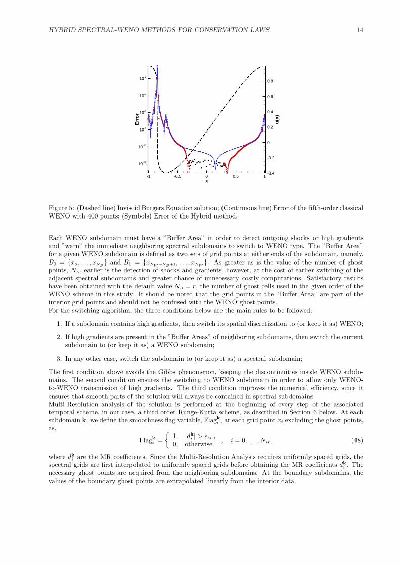
with periodic boundary condition. The initial configuration will quickly evolve into a moving shock, however,at this point we will analyze the pre-shock error in order to show that the superior accuracy of the spectralscheme improves the WENO error as we see in Figure 5. For the Classical WENO method we discretize theinterval [−1, 1] with 400 points. For the Hybrid method, the interval is subdivided into three equal sizedsubdomains, where the middle one, [−0.3, 0.3], is a spectral subdomain. The subdomains configuration iskept fixed, since no shock will arise during the time interval of the experiment.The number of points in the WENO subdomains are the same as the corresponding regions of the classicalWENO, so any increase of accuracy must be due to the spectral subdomain. Note that not only the errorat the spectral subdomain is smaller than the one of the classical WENO, but it also forces the decreasingof the overall error, showing its superior performance and also the conservation properties of the interfaceconditions. Another aspect that should be noticed is the globality of the spectral scheme that can be observedwhen looking to the uniformity of the error at the spectral subdomain.

5.2 The Switching Algorithm

In this section we describe the subdomain switching algorithm. Since we are interested in solving unsteadymoving shocked flows, the subdomains must be able to switch from one type of subdomain to the other, asdictated by the smoothness of the solution and determined by the Multi-Resolution Analysis of Section 4.


x

Err

or

u(x

)

1 0.5 0 0.5 1

1012

1010

108

106

104

102

0.4

0.2

0

0.2

0.4

0.6

0.8

Figure 5: (Dashed line) Inviscid Burgers Equation solution; (Continuous line) Error of the fifth-order classicalWENO with 400 points; (Symbols) Error of the Hybrid method.

Each WENO subdomain must have a ”Buffer Area” in order to detect outgoing shocks or high gradientsand ”warn” the immediate neighboring spectral subdomains to switch to WENO type. The ”Buffer Area”for a given WENO subdomain is defined as two sets of grid points at either ends of the subdomain, namely,B0 = {x0, . . . , xNB

} and B1 = {xNW −NB+1, . . . , xNW}. As greater as is the value of the number of ghost

points, NB, earlier is the detection of shocks and gradients, however, at the cost of earlier switching of theadjacent spectral subdomains and greater chance of unnecessary costly computations. Satisfactory resultshave been obtained with the default value NB = r, the number of ghost cells used in the given order of theWENO scheme in this study. It should be noted that the grid points in the ”Buffer Area” are part of theinterior grid points and should not be confused with the WENO ghost points.For the switching algorithm, the three conditions below are the main rules to be followed:

1. If a subdomain contains high gradients, then switch its spatial discretization to (or keep it as) WENO;

2. If high gradients are present in the ”Buffer Areas” of neighboring subdomains, then switch the currentsubdomain to (or keep it as) a WENO subdomain;

3. In any other case, switch the subdomain to (or keep it as) a spectral subdomain;

The first condition above avoids the Gibbs phenomenon, keeping the discontinuities inside WENO subdo-mains. The second condition ensures the switching to WENO subdomain in order to allow only WENO-to-WENO transmission of high gradients. The third condition improves the numerical efficiency, since itensures that smooth parts of the solution will always be contained in spectral subdomains.Multi-Resolution analysis of the solution is performed at the beginning of every step of the associatedtemporal scheme, in our case, a third order Runge-Kutta scheme, as described in Section 6 below. At eachsubdomain k, we define the smoothness flag variable, Flagk

i , at each grid point xi excluding the ghost points,as,

Flagki =

{1, |dk

i | > εMR

0, otherwise , i = 0, . . . , NW , (48)

where dki are the MR coefficients. Since the Multi-Resolution Analysis requires uniformly spaced grids, the

spectral grids are first interpolated to uniformly spaced grids before obtaining the MR coefficients dki . The

necessary ghost points are acquired from the neighboring subdomains. At the boundary subdomains, thevalues of the boundary ghost points are extrapolated linearly from the interior data.


The algorithm proceeds by checking for each spectral subdomain k and at the Buffer Areas of the neighboringsubdomains k − 1 and k + 1, if any of {Flagk

i , i = 0, . . . , NW}, {Flagk+1i , i = 0, . . . , NB} or {Flagk−1

i , i =NW −NB +1, . . . , NW} is equal to one. If so, it switches subdomain k to a WENO discretization. Otherwise,a spectral discretization is implemented, or kept. These switches require the use of interpolation from aChebyshev grid of points to a uniformly spaced one and vice-versa:

• To switch from the spectral subdomain to the WENO subdomain, the data are interpolated onto theuniformly spaced grid via the spectral interpolation formula.

• To switch from the WENO subdomain to the spectral subdomain, the data are interpolated onto theChebyshev Gauss-Lobatto points via the Lagrangian interpolation polynomial of the same order as theWENO method.

Remark 3 Back and forth switching between WENO and spectral discretizations may occur too frequently forthe same domain when the εMR is marginally set. The dk

i coefficients might oscillate around the parameterεMR in time due to some numerical factors such as dissipation, dispersion and nonlinear effects, or anycombination of such. This pattern of switching can repeat itself for a while until the solution settles downwith a clear definition of the dk

i , which is either greater than or smaller than the MR tolerance εMR. In orderto alleviate such occurrences, one must devise a procedure preventing the switch from WENO to spectral if ithad already occurred recently. However, such procedure must never prevent a spectral to WENO switch, foroscillations and instability might occur.

We end this section proceeding further with the temporal integration of the inviscid Burgers Equation 47to a final time t = 5 where the shock has already developed and performed an entire revolution at theperiodical domain. The numerical results are shown at Figure 6 where we now have partitioned the intervalwith 10 subdomains. Each spectral subdomain uses 17 points, while the WENO ones uses 40 points. Notethat the Hybrid Method was able to compute the exact location of the shock, demonstrating its conservativeproperty.

x

u(x

)

Err

or(x

)

1 0.8 0.6 0.4 0.2 0 0.2 0.4 0.6 0.8 10

0.1

0.2

0.3

0.4

0.5

0.6

0.7

0.8

0.9

1

109

108

107

106

105

104

103

102

101

100

Figure 6: Inviscid Burgers Equation solution; The solution computed by the Hybrid scheme is plotted withsymbols against the exact solution in solid line. The error is plotted in dashed lines. Vertical dashed linesshow the subdomains division.


6 Numerical Experiments

In this section we present numerical experiments with the system of Euler Equations for gas dynamics instrong conservation form:

Qt + Fx = 0, (49)

where

Q = (ρ, ρu, E)T , F = (ρu, ρu2 + P, (E + P )u)T , (50)

and the equation of state

P = (γ − 1)(

E +12ρu2

), γ = 1.4. (51)

In all examples below, the physical domain is partitioned into a fixed number of same size subdomains andthe initial configuration of these subdomains depends on the initial condition under consideration. Spectralsubdomains are discretized with Chebyshev-Gauss-Lobatto collocation points and WENO subdomains usean uniform grid, where the classical fifth order characteristic-wise WENO finite difference is applied. Weshall use the same number of uniformly spaced grid points Nw for all WENO subdomains, as well as thesame number of Chebyshev collocation points Ns at all spectral subdomains, unless noted otherwise. Thedetection of discontinuities and high gradients is performed throuhg a fifth order Multi-Resolution Analysisapplied to the density function ρ. A 16 th order Exponential filter is employed in all spectral subdomains.To evolve in time the ODEs resulting from the semi-discretized PDEs, the third order Total VariationDiminishing Runge-Kutta scheme (RK-TVD) will be used [23]:

~U1 = ~Un + ∆tL(~U )n

~U2 =14

(3~Un + ~U1 + ∆tL(~U1)

), (52)

~Un+1 =13

(~Un + 2~U2 + 2∆tL(~U2)

)

where L is the spatial operator. CFL numbers for the spectral and WENO subdomains are set to be 1 and0.4, respectively. All results of the hybrid method are compared with an exact solution or with a numericalsolution obtained with the classical WENO scheme with the same spatial resolution of the hybrid scheme.This is achieved by using the same number of points for the classical scheme as if all subdomains in thehybrid were of the WENO type ( see Section 5). The main goal of the numerical experiments below is toshow that the Hybrid method obtains equivalent solutions as the classical WENO scheme, however at alower computational cost. This is easily concluded from the facts that spectral discretization is much moreefficient than the finite differences at smooth parts of the solution and that spectral subdomains avoid theexpensive characteristic decomposition of the WENO scheme.In the figures shown for the one dimensional test cases, the spectral and WENO subdomains are those denotedwith squares (�) and triangles (4) symbols respectively. The subdomains are also indicated by verticaldashed lines and major ticks on the x axis. Under each figure, the subdomains configuration is indicated asa sequence of powers of S and W, where the exponent means the number of consecutive subdomains of thesame type. This notation will make easier the counting of subdomain types in the case of a large number ofsubdomains.

6.1 Shock Tube Problems

We first consider the Sod problem of the Compressible Euler equations with initial Riemann data:

(ρ, U, P ) ={

( 0.125, 0, 0.1 ) −5 ≤ x < 0( 1, 0, 1 ) 0 ≤ x < 5 . (53)

The physical domain [−5, 5] is partitioned into 5 equal sudomains. Since the initial condition is discontinuousat the center of the physical domain, the middle subdomain, [−1, 1], is set as WENO (Figure 7(a)). Here,NS = 16 and NW = 110 and the MR tolerance was taken as εMR = 5 × 10−3.


x

Rh

o

5 3 1 1 3 50

0.2

0.4

0.6

0.8

1

x

Rh

o

5 3 1 1 3 50

0.2

0.4

0.6

0.8

1

x

Rh

o

5 3 1 1 3 50

0.2

0.4

0.6

0.8

1

(a) t = 0 , S2W1S2 (b) t = 0.39 S1W2S2 (c) t = 0.54 S1W3S1

x

Rh

o

5 3 1 1 3 50

0.2

0.4

0.6

0.8

1

x

Rh

o

5 3 1 1 3 50

0.2

0.4

0.6

0.8

1

(d) t = 1.46 S1W3S1 (e) t = 2 W4S1

Figure 7: The density profile of the Sod shock tube problem at times (a) t = 0, (b) t = 0.39, (c) t = 0.54, (d)t = 1.46 and (e) t = 2 with 5 subdomains. NS = 16, NW = 110 and εMR = 5 × 10−3. Spectral(�); WENO(4); The solid line is the exact solution.

As time evolves, the initial density discontinuity develops into two jump discontinuities, the leftward movingshock front and contact discontinuity and a rightward moving rarefaction wave, which is discontinuous in thefirst derivative (Figures 7(b) and (c)). Notice that when the discontinuities move on closer to the boundary ofthe WENO subdomain [−1, 1], the neighboring spectral subdomains are switched to WENO ones. At a latertime, the discontinuities have moved further to the left side of the physical domain, however the first andlast subdomains were kept as spectral ones, since none of them has been ”threatened” by the discontinuities.We now consider the 123 problem with initial Riemann data,

(ρ, U, P ) ={

( 1, −2, 0.4 ) −5 ≤ x < 0( 1, 2, 0.4 ) 0 ≤ x ≤ 5 . (54)

The solution consists of two rarefaction waves moving in opposite directions which are generated at thecenter of the physical domain by a discontinuity in the velocity.Using the same setting as the Sod problem discussed in the previous example, we compute the numericalsolution up to t = 1. Figure (8) (d) shows that the middle WENO subdomain [-1,1] is switched to spectralas soon as the rarefaction waves move away from the buffer zones of the neighboring domains. Note alsothat the first and last spectral subdomains have a smaller number of discretization points than the newlycreated spectral subdomain, showing that the Hybrid scheme might also provide quantitative flexibility atthe local discretizations. Non-consecutive WENO subdomains can also have distinct number of grid points.


x

Rh

o

5 3 1 1 3 50

0.2

0.4

0.6

0.8

1

x

Rh

o

5 3 1 1 3 50

0.2

0.4

0.6

0.8

1

x

Rh

o

5 3 1 1 3 50

0.2

0.4

0.6

0.8

1

(a) t = 0 S1W2S1 (b) t = 0.25 S2W1S2 (c) t = 0.29 S1W3S1

x

Rh

o

5 3 1 1 3 50

0.2

0.4

0.6

0.8

1

x

Rh

o

5 3 1 1 3 50

0.2

0.4

0.6

0.8

1

(d) t = 0.62 S1W1S1W1S1 (e) t = 1 S1W1S1W1S1

Figure 8: The density profile of the 123 problem at times (a) t = 0, (b) t = 0.25, (c) t = 0.29, (d) t = 0.62and (e) t = 1 with 5 subdomains. NS = 16, NW = 110 and εMR = 5 × 10−3. Spectral(�); WENO (4); Thesolid line is the exact solution.

6.2 Blastwaves Simulation

The one dimensional Blast waves interaction problem by Woodward and Collela [16] has the following initialprofile

(ρ, U, P ) =

( 1, 0, 1000 ) 0 ≤ x < 0.1( 1, 0, 0.01 ) 0.1 ≤ x < 0.9( 1, 0, 100 ) 0.9 ≤ x ≤ 1.0

. (55)

The initial pressure gradients generate two density shock waves that colide and interact later in time. In thisexperiment, the physical domain is subdivided into 10 subdomains and the number of Chebyshev collocationpoints and WENO uniform grid are Ns = 16 and Nw = 50, respectively. Reflective boundary conditions areapplied at both ends of the physical domain. Figure (9) shows that at the initial times, the expensive WENOdiscretizationS are localized around the density peaks, while the remaining subdomains are spectral. Atintermediate times, the left rarefaction wave spreads around, requiring the use of more WENO subdomains,however, by the end of the simulation, we have more spectral subdomains than WENO ones. It is clearfrom Figure (9) (c) that one could decrease the number of discretization points at the first five spectralsubdomains, or take a step further and merge all the subdomains at a single spectral one, increasing thenumerical efficiency of the algorithm. These improvements will be considered in future implementations ofthe Hybrid method.


x

Rh

o

0 0.1 0.2 0.3 0.4 0.5 0.6 0.7 0.8 0.9 10

1

2

3

4

5

6

7

x

Rh

o

0 0.1 0.2 0.3 0.4 0.5 0.6 0.7 0.8 0.9 10

1

2

3

4

5

6

7

x

Rh

o

0 0.1 0.2 0.3 0.4 0.5 0.6 0.7 0.8 0.9 10

1

2

3

4

5

6

7

(a) t = 0.014 W2S6W2 (b) t = 0.16 S2W3S2W3 (c) t = 0.38 S5W4S1

Figure 9: The density profile of the Blastwave problem at times t = 0.014, t = 0.16 and t = 0.38 with 10subdomains as indicated by the vertical dash lines, NS = 16, NW = 50 and εMR = 5 × 10−3. Spectral (�);WENO (4); The solid line is the solution computed using the classical WENO scheme with 500 points.

6.3 Shock-Entropy Wave Interaction

Consider the one dimensional Mach 3 shock-entropy wave interaction, specified by the following initialconditions:

(ρ, u, P ) ={

( 3.857143, 2.629369, 10.33333 ) −5 ≤ x < −4( 1 + ε sin(kx), 0, 1 ) −4 ≤ x ≤ 15 , (56)

where x ∈ [−5, 15] , ε = 0.2 and k = 5. The solution of this problem consists of shocklets and fine scalesstructures which are located behind a rightgoing main shock. Figures 10–11 show that the hybrid method

x

Rh

o

4 2 0 2 4 6 8 10 12 14

1

2

3

4

5

x

Rh

o

4 2 0 2 4 6 8 10 12 14

1

2

3

4

5

(a) t = 0 S1W2S37 (b) t = 1.5 S4W1S4W1S2W1S27

Figure 10: The density profile of the Mach 3 Shock-Entropy wave interaction at times (a) t = 0, (b) t = 1.5with 40 subdomains, as indicated by the vertical lines. NS = 16, NW = 50 and εMR = 5×10−3. Spectral(�);WENO (4); The solid line is the solution computed with the fifth order WENO scheme with 2000 gridpoints.

is able to capture all the smooth high frequency waves behind the main shock with spectral discretizations.Note that the WENO subdomains are located only at the main shock and at the steep gradients of theN-waves. The hybrid method uses 40 subdomains, with NS = 16 and NW = 50. The solid black line is thesolution computed with the fifth order WENO scheme with 2000 grid points. Figures 11 (b) also show thateven with the great complexity of the solution, less than 30% of the total number of subdomains are of theWENO type.


x

Rh

o

4 2 0 2 4 6 8 10 12 14

1

2

3

4

5

x

Rh

o

4 2 0 2 4 6 8 10 12 14

1

2

3

4

5

(a) t = 3.2 S6W1S2W1S2W2S2W1S2W1S4W1S15 (b) t = 4.5 S7W2S2W1S2W1S2W2S1W2S2W1S8W2S5

Figure 11: The density profile of the Mach 3 Shock-Entropy wave interaction at times (a) t = 3.2 and (b)t = 4.5.

6.4 Shock-Vortex Interaction

We now show some previous results of the Hybrid method in more spatial dimensions. A more detaileddiscussion will be reported at an upcoming article. In this experiment, the multidomain hybrid configurationis applied to a 2D Shock-Vortex interaction. We consider a counter-clockwise rotating vortex centered at(xc, yc), and strength Γ, with a tangential velocity profile [7] given in polar coordinates by:

U (r) =

Γr(r−20 − r−2

1 ) 0 ≤ r ≤ r0 < r1

Γr(r−2 − r−21 ) r0 ≤ r ≤ r1

0 r > r1

, (57)

where r0 = 0.2 and r1 = 1.0. The physical domain (0 ≤ x ≤ 3.9,−2 ≤ y ≤ 2) is partitioned into a 13×10 gridof subdomains. Spectral and WENO subdomains use a 32 × 32 grid of Chebyshev collocation points and a50×50 uniform grid, respectively. The Multi-Resolution analysis is performed with tolerance εMR = 5×10−2.We simulate a Mach 3 shock interacting with the vortex of strength Γ = 0.25 and compare the solutionobtained by the hybrid method with the above setup with a highly resolved solution using the classicalfifth order characteristic-wise WENO finite difference scheme with a 1200 × 1200 grid at final time t = 0.6(Figure 12). The shock and the high gradient regions immediately behind the shock are well captured by theMR analysis, as indicated by the WENO subdomains enclosed with black bounding boxes. The remainingsubdomains are accurately dealt with by the spectral method since all the essential small and large scalestructures of the flow field are correctly represented in the hybrid solution. Once again, the number ofWENO subdomains is far fewer than the spectral ones, resulting in a more efficient algorithm than theclassical WENO scheme.

7 Conclusions

We have presented an one dimensional version of the multi-domain spatial and temporal adaptive HybridSpectral-WENO method for nonlinear system of hyperbolic conservation laws. The physical domain ispartitioned into a grid of subdomains which is either a Chebyshev collocation grid for the spectral method oran uniformly spaced grid for the high order WENO method. High order Multi-Resolution Analysis is usedto measure the smoothness of the solution in a given subdomain and a strategy for switching the subdomainfrom spectral to WENO when the solution becomes non-smooth and vice versa is devised. The Hybridmethod is tested with the standard shock-tube test problems, Shock-Entropy wave interaction problem andthe Blastwave problem. The results are in good agreement with the one computed by the classical fifth orderWENO finite difference method. The switching procedure devised performs well. The Hybrid method is at


x

y

0 1 2 3 42

1

0

1

2

x

y

0 1 2 3 42

1

0

1

2

Figure 12: Density contour of the Shock-Vortex interaction with Mach number Ms = 3 and vortex strengthΓ = 0.25 at t = 0.6. Hybrid (Left); Classical WENO (Right). WENO subdomains are denoted by boundingboxes.

least 3-4 times faster than the classical fifth order characteristic-wise WENO finite difference method for theproblems tested here resulting in a good speedup and efficient method for shocked flow. Timing results willbe given in the upcoming paper in the two dimensional extension of the Hybrid method, which is a muchmore meaningful measure than the one dimensional one.Currently, we are investigating the role of the Multi-Resolution Tolerance εMR and its effects on the Hybridsolution. Furthermore, the implementation of the smoothness measurement in the spectral subdomains canbe improved and is under investigation. We plan to extend the Hybrid method to nonlinear hyperbolicconservation laws system in higher dimensions and with higher order WENO scheme.

8 Acknowledgments

The first author has been supported by CNPq, grant 300315/98-8. The second author gratefully acknowledgesthe support of this work by the AFOSR under contract number F49620-02-1-0113 and FA9550-05-1-0123.

References

[1] W. S. Don and A. Solomonoff, Accuracy and Speed in Computing the Chebyshev Collocation Derivative,SIAM J. Sci. Comp. 16, No. 6 pp. 1253–1268 (1995)

[2] D. Gottlieb and S. A. Orszag, Numerical Analysis of Spectral Methods: Theory and Applications, CBMSconference Series in Applied Mathematics 26, SIAM, (1977)

[3] D. Gottlieb, C. W. Shu, A. Solomonoff and H. Vandeven, On the Gibbs phenomenon I: recoveringexponential accuracy from the Fourier partial sum of a non-periodic analytic function, J. Comp. andAppl. Math. 43, pp. 81-98 (1992)

[4] D. Gottlieb and C. W. Shu, On the Gibbs phenomenon V: recovering exponential accuracy from collo-cation point values of a piecewise analytic function, Numerische Mathematik 71, pp. 511–526 (1995)

[5] D. Gottlieb and E. Tadmor, Recovering pointwise values of discontinuous data within Spectral accuracy,Progress and Supercomputing in Computational Fluid Dynamics, ed. E. Murman, et al., Proc. of U.S.–Israel Workshop, pp. 357–375 (1985)

[6] A. Harten, UCLA CAM Report 93-03, March 1993


[7] D. A. Kopriva, A Multidomain Spectral Collocation Computation of the Sound Generated by a Shock-Vortex Interaction, Computational Acoustics: Algorithms and applications 2, D. Lee and M. H. Schultz(eds.), Elsevier Science Publishers B. V., North Holland, IMACS (1988)

[8] P. D. Lax, Accuracy and resolution in the computation of solutions of linear and nonlinear equations,in Recent advances in Numerical Analysis, Proc. Symp., Mathematical Research Center, University ofWisconsin, Academic Press, pp. 107–117 (1978)

[9] S. P. Pao and M. D. Salas, A Numerical Study of Two-Dimensional Shock-Vortex Interaction, AIAAPaper, pp. 81–1205 (1981)

[10] E. Tadmor, Convergence of spectral methods for nonlinear conservation laws, SINUM 26, pp. 30–44(1989)

[11] Y. Maday, S. O. Kaber and E. Tadmor, Legendre Pseudospectral Viscosity Method for Nonlinear Con-servation Laws, SIAM J. Numer. Anal. 30, pp. 321–342 (1993)

[12] H. Vandeven, Family of spectral filters for discontinuous problems, J. Sci. Comp. 24, pp. 37–49 (1992)

[13] W. S. Don, Numerical Study of Pseudospectral Methods in Shock Wave Applications, J. Comp. Phys.110, pp. 103–111, 1994

[14] H. S. Ribner, Shock-Turbulence Interaction and the Generation of Noise, NACA Report 1233, 1955

[15] K. Sebastian, Multi domain WENO finite difference method with interpolation at sub-domain interfaces,J. Sci. Comput. 19, pp. 405–438 (2003)

[16] P. Woodward and P. Collela, The numerical simulation of two dimensional fluid flow with strong shocks,J. Comp. Phys. 54 (1984), pp. 115–173

[17] N. Adams and K. Shariff high-resolution hybrid compact-ENO scheme for shock-turbulence interactionproblems, J. Comp. Phys. 127, pp. 27–51 (1996)

[18] B. Bihari and A. Harten, Multiresolution schemes for the numerical solution of 2-D Conservation Laws,SIAM J. Sci. Comp. 18, Vol. 2, pp. 315-354 (1997)

[19] A. Choen, S. M. Kaber, S. Muller and M. Postel, Fully Adaptive Multiresolution Finite Volume Schemesfor Conservation Laws, Math. Compuutt. 72, No. 241, pp. 183–225 (2001)

[20] I. Daubechies, Ten Lectures on Wavelets, CBMS-NSF Regional Conferences Series in Applied Mathe-matics, SIAM, Capital City Press, Montpellier, Vermont (1992)

[21] A. Harten, High Resolution Schemes for Hyperbolic Conservation Laws, Comput. Phys. 49, pp. 357–393(1983)

[22] A. Harten, Adaptive Multiresolution Schemes for Shock Computations, Comput. Phys. 115, pp. 319–338(1994)

[23] G. S. Jiang and C. W. Shu, Efficient Implementation of Weighted ENO Schemes, J. Comp. Phys. 126,pp. 202–228 (1996)

[24] S. Pirozzoli, Conservative Hybrid Compact-WENO schemes for Shock-Turbulence Interaction, J. Comp.Phys. 178, No. 1, pp. 81–117 (2002)

[25] C. W. Shu and S. Osher, Efficient Implementation of Essentially Non-oscillatory Shock-CapturingSchemes, II, J. Comp. Phys. 83, No. 1, pp. 32–78 (1989)

[26] M. S. Min, M. S. Kaber and W. S. Don, Fourier-Pade approximations and filtering for the spectral sim-ulations of incompressible Boussinesq convection problem, Math. Comput., Publications du LaboratorieJacques-Louis Lions, R03021, Math. Comput., accepted for publication.


[27] J. H. Jung and B. D. Shizgal, Towards the Resolution of the Gibbs phenomenon, J. Comput. AppliedMath. 161, No. 1, pp. 41-65 (2003)

[28] J. H. Jung and B. D. Shizgal, Generalization of the Inverse Polynomial Reconstruction Method in theResolution of the Gibbs Phenomena, J. Comput. Applied Math. 172, No. 1, pp. 131-151 (2004)

multi-domain hybrid spectral-weno methods for …bcosta/papers/hybrid1d.pdf · multi-domain hybrid...

Documents