hedging barrier options through a log-normallocal …mssanz.org.au/modsim2017/e3/ning.pdf ·...

Hedging Barrier Options through a Log-Normal LocalStochastic Volatility Model

Wei Ning a, G. Leea, N. Langrenea

aCSIRO DATA61-Real Options and Financial Risk, Clayton, Victoria, 3168Email: [email protected]

Abstract: In the equity and foreign exchange (FX) markets, there has been a shift towards using non-affine pricing models as these have been shown to produce more realistic volatility distributions and more accurately capture market dynamics. One such non-affine model is the Inverse Gamma model, which we have incorporated into a Local-Stochastic Volatility (LSV) model termed the Log-normal-LSV (LN-LSV) that can, once calibrated, accurately reproduce market prices of exotic options Langrene and Zhu [2016]. The LN-LSV model is a non-parametric combination of local volatility and stochastic volatility models, in which both the spot price and stochastic volatility follow log-normal processes. The LN-LSV model is calibrated using both the market-traded implied volatility surface and market exotic option prices.

However, while the accurate pricing of exotic options is necessary for good pricing model performance, it is also necessary for models to perform in risk management applications, where hedges are entered into to minimise risk. Therefore, the accurate calculation of the derivatives of the option price with respect to the asset or volatility (the Greeks) is also necessary for good model performance.

This paper aims to characterise the hedging performance of the Log-normal Local-Stochastic Volatility model for a variety of hedging instruments using an historical dataset consisting of daily spots and volatility surfaces for the EUR/USD market over a five-year time period. We use delta-gamma hedging for different barrier options under the LN-LSV model and compare the hedging performance with that of the Black-Scholes (BS) model. Then we use the numerical results to demonstrate that the LN-LSV model is more effective than the BS model.

We use five types of reverse knock-out options as test cases over a time period of five years. On each trading day from 2007 to 2011, the five options are firstly priced using the LN-LSV model. After pricing, each option is hedged daily until the expiry date of the option using a delta-gamma neutral scheme under both the LN-LSV and BS models. To measure the hedging performance, each profit-loss outcome forms one point of the P&L distribution. During Jan 2007 to Dec 2011, the profit and loss of a total of 1100 traded options for each option type forms the P&L distribution. Compared to the Black-Scholes model, the P&L distribution of the numerical results from LN-LSV model is more symmetric and is less likely to have extreme profit-loss outliers. Thus it produces more superior hedging performance.

Keywords: Barrier option, Delta-Gamma hedging, Black-Scholes model, Log-Normal Local Stochastic Volatility model, hedging performance

22nd International Congress on Modelling and Simulation, Hobart, Tasmania, Australia, 3 to 8 December 2017 mssanz.org.au/modsim2017

770

1 INTRODUCTION

The dynamic hedging of financial options can be improved when taking higher order Greeks into account.The most widely used first order Greek in hedging is Delta, the first order derivative of the option price withrespect to the spot price. Previous work concerned with the delta hedging performance has been carried outby Boyle and Emanuel [1980]. They rebalance the portfolio at discrete times using the Black-Scholes modelto ensure the hedged portfolio remains delta-neutral (i.e., the delta of the portfolio is zero at each rebalancingstep). Hull and White [1987] analyse the key factors affecting the performance of delta hedging in a stochasticvolatility environment. Researchers also use higher order Greeks to quantify different aspects of risk in optionportfolios and attempt to make the portfolio immune to big changes in the underlying asset price. Kurpieland Roncalli [1998] implemented both a pure delta hedge and a delta-gamma hedge the under the frameworkof Black-Scholes. Under a delta-gamma hedging scheme, both the delta and gamma of the portfolio remainneutral at each rebalancing step. The authors show that the delta-gamma hedging strategy improves theperformance of a discrete rebalanced delta hedging and reduces the standard deviations of the net hedge costs.Then they show that in the case of delta-gamma-vega hedging scheme, where vega is also kept neutral, thestochastic volatility model outperforms the strategy based on the BS methods under some conditions.

A further improvement to the class of stochastic volatility models, where the volatility follows an independentstochastic process Gatheral [2011], is the class of Local-Stochastic Volatility (LSV) models. The class ofLSV models combines the advantages of both the local volatility model (reproducing the market implied volsurface) and stochastic volatility models (reproducing market dynamics). The LN-LSV model used in thispaper uses a log-normal process for the stochastic volatility component Zhu et al. [2015]. Since the LN-LSVmodel is more accurate in capturing the underlying dynamics of foreign-exchange spot in practise, it has beenwidely used by tier-one global banks for exotic option valuation in the foreign-exchange options market.

To assess the replication ability of LN-LSV model, a delta hedging backtest has been implemented Denes[2016]. The authors followed the path in Ling and Shevchenko [2016] which compares delta hedging perfor-mance under Local Volatlity and BS model. Their results show that the delta hedging performance of boththe LN-LSV model and BS model are very similar. However, a delta neutral portfolio can still have non-zerogamma which is the second order derivative of option price with respect to spot price. When the spot pricefluctuates widely, the unhedged movements of higher order Greeks can cause significant profit or loss. In orderto compare the different hedging performances between different models, we compute the reverse knock-outbarrier option prices and their first and second-order Greeks using LN-LSV and BS model respectively. Wealso discuss the practical implementation and the choice of hedging instruments.

In this paper, we first introduce the LN-LSV model in Section 2. We then propose the delta-gammahedging scheme for the following five types reverse knock-out options using LN-LSV: 10∆CallBarrier,25∆CallBarrier, ATMCallBarrier, 25∆PutBarrier and 10∆PutBarrier in Section 3. In section 4, we useboth the LN-LSV and the BS model to price these options and compute their Greeks respectively on eachtrading day through the life cycle. We then analyse and compare the hedging performance of these two models.

2 LOG-NORMAL LOCAL-STOCHASTIC VOLATILITY MODEL

The LN-LSV model is a non-parametric combination of local volatility and stochastic volatility models. Inthis model, we assume that both spot price St and volatility σt follow their log-normal stochastic processesZhu et al. [2015].

dSt = [rd(t)− rf (t)]Stdt+ L(St, t)σtStdW1t , S0 = s,

dσt = κ(θ − σt)dt+ λσtdW2t , σ0 = v,

E[dW 1t · dW 2

t ] = ρdt. (1)

where rd(t) is domestic interest rate and rf (t) is foreign interest rate, both of which are assumed to be ofterm structures. We assume that the other stochastic parameters κ, θ, λ and ρ in LN-LSV model also haveterm structures. L(St, t), termed the leverage function, representing the ratio between local volatility and theexpectation of stochastic volatility conditional on the current asset price St. We calibrate the leverage functionL numerically using market data.

Ning et al., Hedging Barrier Options through a Log-Normal Local Stochastic Volatility Model

771

Table 1. Reverse knock-out options10∆Call Barrier A reverse Up-And-Out Call equivalent to a 10∆Call Barrier = 1.025K25∆Call Barrier A reverse Up-And-Out Call equivalent to a 25∆Call Barrier = 1.025KATM Call Barrier A reverse Up-And-Out Call equivalent to a ATM Call Barrier = 1.025K10∆Put Barrier A reverse Down-And-Out Put equivalent to a 10∆Put Barrier = 0.975K25∆Put Barrier A reverse Down-And-Out Put equivalent to a 25∆Put Barrier = 0.975K

3 DYNAMIC DELTA-GAMMA HEDGING

In constructing the Delta-Gamma hedging scheme, we make the assumptions that the market is arbitrage free,perfectly liquid and frictionless, and we can take any fractional short or long position in any asset. In order tokeep the portfolio Delta-Gamma neutral, we need to rebalance the hedging instruments on each trading day.

3.1 Delta-Gamma Neutral Hedging

Each barrier option is Delta-Gamma hedged daily using both the LN-LSV model and the BS model untilthe expiry. For each barrier option, we construct a delta-gamma neutral portfolio which contains a shortposition NO of the barrier option, a long position Nh of hedging instrument and NS underlying asset. Whenrebalancing, a Delta-Gamma neutral portfolio should satisfy the following constraints:

∆Portfolio = ∆SNS −∆ONO + ∆hNh = 0, (2)ΓPortfolio = ΓSNS − ΓONO + ΓhNh = 0. (3)

where Nh and NS are the net positions of hedging instrument and stock in this portfolio, ∆O and ΓO denotedelta and gamma of the barrier option, ∆h and Γh denote delta and gamma of the hedging instrument respec-tively. For the gamma and delta of the stocks, we have ΓS = 0 and ∆S = 1. Assuming the short position ofbarrier option NO = 1, we can solve for Nh and NS from the linear system (2,3). Therefore we have:

Nh =ΓO

Γh, NS = ∆O −∆h

ΓO

Γh. (4)

3.2 Hedging Instrument

In this paper, we focus on hedging the five reverse knock-out barrier options listed in Table (1). The maturitiesof these options are 3 months.

To select the hedging instrument, Molchan and Rouah hedged a one-month Up-and-Out call option with avanilla call of identical features Molchan and Rouah [2011]. Raju [2012] applied Delta-Gamma hedgeing forvanilla call options by another vanilla call option with a different strike using BS model. In 2009, Engelmannet al. proposed Delta-Vega hedging on Down-and-Out barrier options where they adopted ATM vanilla optionas the hedging instrument Engelmann et al. [2009]. Besides dynamic hedging, Derman et al. introduced statichedging through a portfolio of vanilla options with various strikes and maturities Derman et al. [1995].

From the these papers, we can see that vanilla option is a reasonable candidate as our hedging instrument.First of all, vanilla options are similar to barrier options except when the barrier is triggered. Secondly,a combination of vanilla options with different strikes can generate any desirable piecewise linear payoffs.Furthermore, the Delta and Gamma of vanillas are straightforward to compute and well-behaved Derman andKani [1997]. The hedging instruments used in this paper are listed in Table 2. We select vanilla options as thehedging instrument with the same maturities and strikes as the barrier options.

3.3 Delta-gamma Hedging

We rebalance each portfolio daily until expiry. Since the interest is accumulated continuously, when Mondayis the trading day, 3-day ( Friday and weekend) interest should be accrued in the portfolios, otherwise 1-dayinterest is applied Ling and Shevchenko [2016]. Let {t}i denote the trading days where i ∈ {1, ..., N}, and Nis the total number of trading days from time 0 to T . C is the price of barrier option hedged at time t0, Si isthe price of underlying stock at time ti, Hi is the price of hedging instrument (vanilla option) at time ti. N i

h

and N iS are net positions of hedging instrument and stock in the portfolio at time ti, defined as Equation (4).

We test the hedging performance with the following steps:


772

Table 2. Hedging instruments in LN-LSV and BS modelTarget Barrier Options Hedging Instrument

10∆Call Barrier Vanilla 10∆Call25∆Call Barrier Vanilla 25∆CallATM Call Barrier Vanilla ATM Call10∆Put Barrier Vanilla 10∆Put25∆Put Barrier Vanilla 25∆Put

1. At t0, we short 1 unit barrier option and long N0s stock and N0

h hedging instrument. The cash positionat initial time t0 is: P0 = C −N0

sS0 −N0

hH0.

2. At the next trading day t1, we start the first rebalancing by longing N1S shares and N1

h hedging instru-ment, thus this results in the change (N0

S −N1S)S1 + (N0

h −N1h)H1. At the same time, the interest

accrued / charged on cash position P0 equals to (eard(t0) − 1)P0 and dividend yield received / paid onunderlying stock is (earf (t0)−1)N0

SS0, where a is the time (in years) between t0 to t1. If trading day t1

is a Monday, then a = 3/365, otherwise, a = 1/365. To sum up the changes in the portfolio, we get thecash position at t1: P1 = P0 +(eard(t0)−1)P0 +(earf (t0)−1)N0

SS0 +(N0

S−N1S)S1 +(N0

h−N1h)H1.

3. On the i-th trading day ti, where i ∈ {1, ..., N − 1}, the cash position is given byPi = eard(ti−1)Pi−1 + (earf (ti−1) − 1)N i−1

S Si−1 + (N i−1S −N i

S)Si + (N i−1h −N i

h)Hi.

4. At maturity tN = T , we sell both underlying shares and hedging instrument. The final cash positionPN = eard(tN−1)PN−1 + (earf (tN−1) − 1)NN−1

S SN−1 +NN−1S SN +NN−1

h HN . One the other side,the payoff of the barrier option is X = max(0, SN −K) for call options and X = max(K − SN , 0)for put options if it is not knocked out, otherwise X = 0.

5. At time expiry T , the hedging error is PN −X because of the short position of barrier option.

4 NUMERICAL TEST

In this section, we backtest the performance of delta-gamma hedging using historic daily EURUSD data from2007/01/01 to 2011/12/30. These market data include: the spot price, implied volatilities for at the money(ATM) options, 10 and 25 delta risk reversals, 10 and 25 delta butterflies and zero coupon rates for the domestic(USD) and foreign (EUR) currencies. From these data, we can calculate strikes of the options from BS formula,and interpolate market implied volatilities using natural cubic spline Press [2007] for each trading day.

Figures 1 to 5 depict the profit and loss (P&L) distributions of Delta-Gamma hedging under frameworks of BSand LN-LSV models. The sample means, standard deviations and other statistics for these 5 barrier optionsare summarised in Tables (3 - 7).

Table 3. 10∆CallBarrier SummariesModel Mean. Median. Max Min Standard Dev. Skewness Kurtosis

BS -0.000218 1.72E-07 0.01941 -0.037906 0.003015 -5.726914 60.25944LN-LSV -0.000246 2.08E-05 0.02034 -0.041326 0.003377 -4.795989 48.61074

Table 4. 25∆CallBarrier SummariesModel Mean. Median. Max Min Standard Dev. Skewness Kurtosis

BS -0.00761 -0.000105 0.293873 -4.998658 0.166492 -26.85515 767.2382LN-LSV -0.001707 -0.000205 0.016951 -0.155152 0.007682 -10.94762 185.6279


773

Figure 1. P&L distribution for 10∆CallBarrier Figure 2. P&L distribution for 25∆CallBarrier

Figure 3. P&L distribution for ATMCallBarrier

Table 5. ATMCallBarrier SummariesModel Mean. Median. Max Min Standard Dev. Skewness Kurtosis

BS -0.009302 -0.00017 0.038319 -5.179844 0.210417 -23.47105 553.3903LN-LSV -0.000516 -5.48E-05 0.017902 -0.242595 0.010443 -21.66694 494.7996

Table 6. 25∆PutBarrier SummariesModel Mean. Median. Max Min Standard Dev. Skewness Kurtosis

BS -0.000809 -4.86E-05 0.004682 -0.043284 0.004064 -6.408469 48.63383LN-LSV -0.000936 -0.000108 0.004846 -0.041772 0.004286 -5.988037 42.52505

Table 7. 10∆PutBarrier SummariesModel Mean. Median. Max Min Standard Dev. Skewness Kurtosis

BS -0.000103 8.25E-06 0.013338 -0.036021 0.002469 -8.311014 105.2769LN-LSV -0.00024 -1.88E-05 0.009129 -0.041599 0.002633 -9.492582 116.838


774

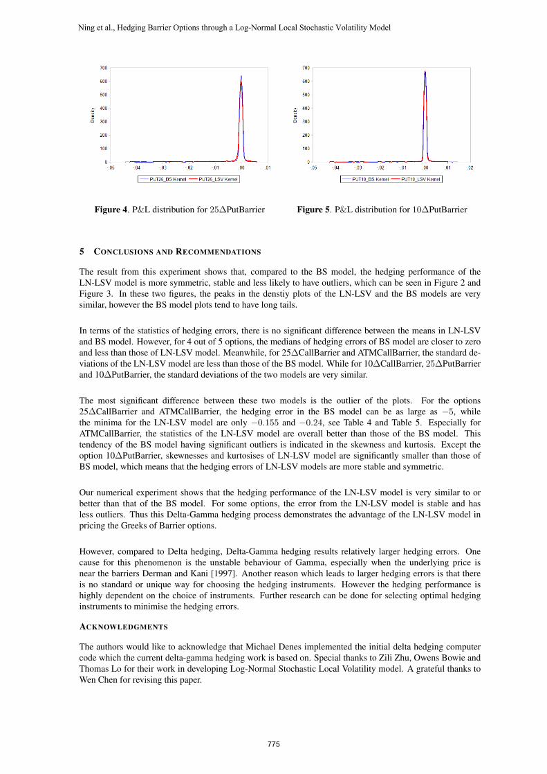
Figure 4. P&L distribution for 25∆PutBarrier Figure 5. P&L distribution for 10∆PutBarrier

5 CONCLUSIONS AND RECOMMENDATIONS

The result from this experiment shows that, compared to the BS model, the hedging performance of theLN-LSV model is more symmetric, stable and less likely to have outliers, which can be seen in Figure 2 andFigure 3. In these two figures, the peaks in the denstiy plots of the LN-LSV and the BS models are verysimilar, however the BS model plots tend to have long tails.

In terms of the statistics of hedging errors, there is no significant difference between the means in LN-LSVand BS model. However, for 4 out of 5 options, the medians of hedging errors of BS model are closer to zeroand less than those of LN-LSV model. Meanwhile, for 25∆CallBarrier and ATMCallBarrier, the standard de-viations of the LN-LSV model are less than those of the BS model. While for 10∆CallBarrier, 25∆PutBarrierand 10∆PutBarrier, the standard deviations of the two models are very similar.

The most significant difference between these two models is the outlier of the plots. For the options25∆CallBarrier and ATMCallBarrier, the hedging error in the BS model can be as large as −5, whilethe minima for the LN-LSV model are only −0.155 and −0.24, see Table 4 and Table 5. Especially forATMCallBarrier, the statistics of the LN-LSV model are overall better than those of the BS model. Thistendency of the BS model having significant outliers is indicated in the skewness and kurtosis. Except theoption 10∆PutBarrier, skewnesses and kurtosises of LN-LSV model are significantly smaller than those ofBS model, which means that the hedging errors of LN-LSV models are more stable and symmetric.

Our numerical experiment shows that the hedging performance of the LN-LSV model is very similar to orbetter than that of the BS model. For some options, the error from the LN-LSV model is stable and hasless outliers. Thus this Delta-Gamma hedging process demonstrates the advantage of the LN-LSV model inpricing the Greeks of Barrier options.

However, compared to Delta hedging, Delta-Gamma hedging results relatively larger hedging errors. Onecause for this phenomenon is the unstable behaviour of Gamma, especially when the underlying price isnear the barriers Derman and Kani [1997]. Another reason which leads to larger hedging errors is that thereis no standard or unique way for choosing the hedging instruments. However the hedging performance ishighly dependent on the choice of instruments. Further research can be done for selecting optimal hedginginstruments to minimise the hedging errors.

ACKNOWLEDGMENTS

The authors would like to acknowledge that Michael Denes implemented the initial delta hedging computercode which the current delta-gamma hedging work is based on. Special thanks to Zili Zhu, Owens Bowie andThomas Lo for their work in developing Log-Normal Stochastic Local Volatility model. A grateful thanks toWen Chen for revising this paper.


775

REFERENCES

Boyle, P. P. and D. Emanuel (1980). Discretely adjusted option hedges. Journal of Financial Economics 8(3),259–282.

Denes, M. C. (2016). Hedging fx risk through a log-normal local-stochastic volatility model.

Derman, E., D. Ergener, and I. Kani (1995). Static options replication. The Journal of Derivatives 2(4), 78–95.

Derman, E. and I. Kani (1997). The ins and outs of barrier options: Part 1. Derivatives Quarterly 3, 73–80.

Engelmann, B., M. R. Fengler, and P. Schwendner (2009). Hedging under alternative stickiness assumptions:an empirical analysis for barrier options. The Journal of Risk 12(1), 53.

Gatheral, J. (2011). The volatility surface: a practitioner’s guide, Volume 357. John Wiley & Sons.

Hull, J. and A. White (1987). Hedging the risks from writing foreign currency options. Journal of Internationalmoney and Finance 6(2), 131–152.

Kurpiel, A. and T. Roncalli (1998). Option hedging with stochastic volatility.

Langrene, N. Lee, G. and Z. Zhu (2016). Switching to non-affine stochastic volatility: A closed-form expan-sion for the inverse gamma model. International Journal of Theoretical and Applied Finance 19, 1650031.

Ling, T. G. and P. V. Shevchenko (2016). Historical backtesting of local volatility model using aud/usd vanillaoptions. The ANZIAM Journal 57(03), 319–338.

Molchan, J. and F. D. Rouah (2011). Where?s my delta? The Journal of Wealth Management 13(4), 68–76.

Press, W. H. (2007). Numerical recipes 3rd edition: The art of scientific computing. Cambridge universitypress.

Raju, S. (2012). Delta gamma hedging and the black-scholes partial differential equation (pde). Journal ofEconomics and Finance Education 11(2).

Zhu, Z., G. Lee, N. Langrene, B. Owens, and L. Thomas (2015). Pricing barrier options with a log-normallocal- stochastic volatility model.


776

hedging barrier options through a log-normallocal …mssanz.org.au/modsim2017/e3/ning.pdf ·...

Documents