happiness and productivity - École normale...

Happiness and Productivity

Andrew J. Oswald, Eugenio Proto and Daniel Sgroi

Department of EconomicsUniversity of Warwick

CoventryCV4 7AL

United Kingdom

PRELIMINARY WORK

28 November 2008

Keywords: Labor productivity; emotions; well-being; happiness; positiveaffect; experimental economics.

Corresponding author: [email protected].

Address: Department of Economics, University of Warwick, Coventry CV47AL, United Kingdom.

Telephone: (+44) 02476 523510

Acknowledgements: For fine research assistance and discussions, we thankMalena Digiuni, Alex Dobson and Lucy Rippon. For helpful suggestions,we thank Alain Cohn, Ernst Fehr, Bruno Frey, Amanda Goodall, Alice Isen,Michel Marechal, Aldo Rustichini, Daniel Schunk and Tanya Singer.Oswald is grateful to the University of Zurich for a visiting professorship,and to the ESRC for research support.

1

Abstract

Little is known by economists about how emotions affect productivity. To make

persuasive progress, some way has to be found to assign people exogenously to

different feelings. We design a randomized trial. In it, some subjects have their

happiness levels increased, while those in a control group do not. A rise in happiness

leads to greater productivity in a paid piece-rate task. The effect is large; it can be

replicated; it exists in male and female subsamples; and it is not a reciprocity effect.

We discuss the implications for economics.

2

Introduction

There is a large economics literature on individual and economy-wide

productivity. There is also a fast-growing one on the measurement of individuals’

mental well-being. Yet economists know little about the interplay between emotions

and human productivity. Although people’s happiness and effort decisions seem

likely to be deeply intertwined, we lack evidence on whether, and how, they are

causally connected.

This paper seeks to make two contributions. First, it attempts to alert

economists to a psychology literature in which happiness (or more precisely what

psychologists describe as positive affect) has been shown to be associated with higher

human performance. Here the work of the psychologist Alice Isen has been

particularly important. The second contribution of the paper is to design and perform

an empirical inquiry that has not been done in the psychology literature. It addresses

a question of particular interest to economists (and perhaps to policy-makers). Does

happiness make people more productive in a paid task? We provide evidence -- in a

standardized piece-rate setting with otherwise fairly well-understood properties -- that

it does.

Argyle (1989 a,b) points out that little is known about how life satisfaction

affects productivity, but that there is some (mixed) evidence that job satisfaction

shows ‘modestly positive correlations’ with measures of worker productivity. Wright

and Staw (1999) examine links between worker affect and supervisors’ ratings of

workers, and, depending on the affect measure, find rather mixed results. In contrast

to our paper, Sanna et al (1996) argue that those in a negative mood put forth the most

effort. Amabile et al (2005) finds that happiness appears to provoke greater

creativity.

We shall not distinguish in any stark way between happiness and ‘mood’. We

take the distinction, in a short run experiment as ours, to be largely semantic or

philosophical. Nor shall we discuss the possibility that other stimuli such as music,

alcohol or sheer relaxation time – all mentioned by readers of early drafts – could

have the same or equivalent effects.

Theory: A model of work and worrying

Consider the following simple model. Its main result, put intuitively, emerges

from internal resource-allocation by the worker. In the model, an initial happiness

3

shock raises the psychological resources available to a worker. At the margin, this

shock frees an overall energy constraint. That in turn allows a worker to devote more

effort to solving problems for pay and to switch away from worrying about other

distractions.

Let the worker’s (randomly distributed) ability be z. This has a density

function f(z). Denote u as utility. Denote p as the piece-rate level of pay. Let e be

the energy the worker devotes to solving the tasks at work. Let w be the energy the

worker devotes to ‘worrying’ about the job and other things. Assume R is the

worker’s psychological resources. Hence (e + w) is less than or equal to R.

Let u be the utility from working, and assume it depends on both the worker’s

earnings and the effort from solving work problems. Let v be the utility from

worrying. Worrying can be thought of as generalized concern for issues in the

worker’s life that need his or her cognitive attention. In a paid-task setting, it might

simply be stress about the possibility of failure at the task. But, more broadly, it can

also be a general form of distraction from the job at hand. Perhaps it might be

realistic to think of a worker as alternating, during the working day, between

concentrating on the task and feeling anxious about his or her job and life.

Assume there is an initial happiness shock, h.

People therefore solve the problem: Choose work-energy e to

Maximize ),()(),,,( hwvdzzfzhepu

subject to weR .

The first-order condition for a maximum in this problem is

0 we vEu . (1)

A comparative-static result of particular interest is the response of productivity, given

by work effort e, to a rise in the initial happiness shock, h. It is determined in a

standard way: The sign of de*/dh takes the sign of the cross partial of the maximand,

so:

Sign de*/dh takes the sign of wheh vEu . (2)

4

Without more restrictions, this sign could be positive or negative. The happiness

shock could increase or decrease the amount of work done on the maths task.

To get some insight into the likely outcome, consider simple forms of these

functions. Assume that workers know their own productivity, so are not subject to the

uncertainty, and that R is normalized to unity. Also set z to unity for simplicity.

Assume u and v are both concave functions.

An additively separable case

Assume additive separability. Then, assuming the worker gets the h happiness shock

whether or not she subsequently works or worries, the worker solves

Maximize hevpeu 2)1()( (3)

and hence at an interior maximum

0)1()( evppeu . (4)

This is a useful benchmark case. Here, the optimal work effort e* is independent of

the happiness shock, h. As h rises or falls, the marginal return to effort is unaffected.

A concavity case

A more plausible form of utility function has the happiness shock operating

within a concave form. Here the worker solves

Maximize )1()( hevhpeu

which is the assumption that h is a shift variable inside the utility function itself,

rather than an additive part of that function.

Now the first-order condition is

0)1()( hevphpeu . (5)

In this case, the optimal level of energy devoted to solving work problems, e*, does

depend on the level of the happiness shock, h.

The sign of de*/dh now takes the sign of )1()( hevphpeu .

5

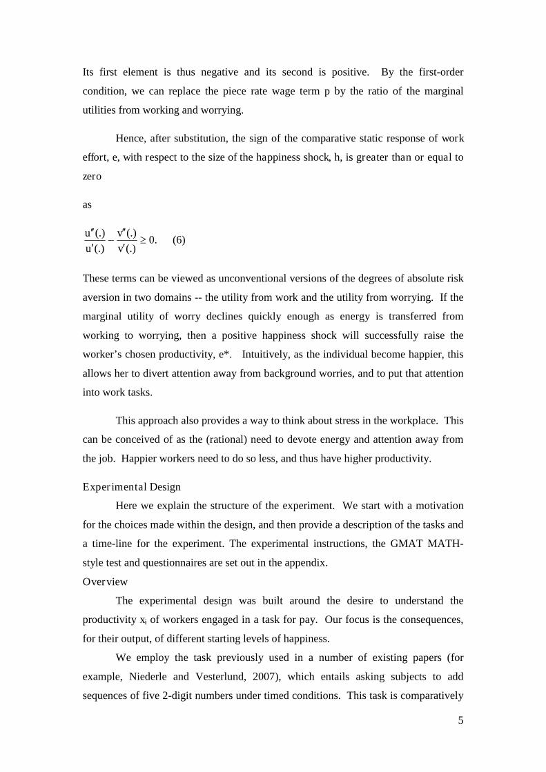
Its first element is thus negative and its second is positive. By the first-order

condition, we can replace the piece rate wage term p by the ratio of the marginal

utilities from working and worrying.

Hence, after substitution, the sign of the comparative static response of work

effort, e, with respect to the size of the happiness shock, h, is greater than or equal to

zero

as

.0(.)

(.)

(.)

(.)

v

v

u

u(6)

These terms can be viewed as unconventional versions of the degrees of absolute risk

aversion in two domains -- the utility from work and the utility from worrying. If the

marginal utility of worry declines quickly enough as energy is transferred from

working to worrying, then a positive happiness shock will successfully raise the

worker’s chosen productivity, e*. Intuitively, as the individual become happier, this

allows her to divert attention away from background worries, and to put that attention

into work tasks.

This approach also provides a way to think about stress in the workplace. This

can be conceived of as the (rational) need to devote energy and attention away from

the job. Happier workers need to do so less, and thus have higher productivity.

Experimental Design

Here we explain the structure of the experiment. We start with a motivation

for the choices made within the design, and then provide a description of the tasks and

a time-line for the experiment. The experimental instructions, the GMAT MATH-

style test and questionnaires are set out in the appendix.

Overview

The experimental design was built around the desire to understand the

productivity xi of workers engaged in a task for pay. Our focus is the consequences,

for their output, of different starting levels of happiness.

We employ the task previously used in a number of existing papers (for

example, Niederle and Vesterlund, 2007), which entails asking subjects to add

sequences of five 2-digit numbers under timed conditions. This task is comparatively

6

simple but is taxing under pressure. It might be thought of as representing in a highly

stylized way an iconic white-collar job: both intellectual ability and effort are

rewarded.

Since we are trying to evaluate the relationship between happiness and

productivity, we wish ideally to disentangle the effort component and ability

component. To this end, we also included two control variables that we hoped would

capture underlying exogenous but heterogeneous ability as opposed to effort --

although we were also open to the possibility that changes in underlying happiness

might induce shifts in ability or change the nature of the interaction between ability

and effort to alter overall productivity. Our control variables came from (i) requiring

our subjects to do a brief GMAT MATH-style test (5 multiple choice questions)

along similar lines to that of Gneezy and Rustichini (2000) and (ii) obtaining

information in a final questionnaire to allow us to construct a measure of subjects’

prior exposure to mathematics. The aim was to allow us to control for heterogeneous

ability levels.1

A key concern was to examine the consequences that happiness has for

productivity (be it through effort or ability). We therefore needed some means of

inducing an exogenous rise in happiness. The psychology literature offers evidence

that movie clips (through their joint operation as a form of audio and visual stimulus)

are a means of doing so. They exogenously alter people’s feelings and mood. For

example, Westermann et al (1996) provides a nice meta-analysis of the methods

available.

We used a 10-minute clip based on composite sketches taken from various

comedy routines enacted by a well-known British comedian. In order to ensure that

the clip and subjects were well matched, we restricted our laboratory pool to subjects

of an English background who had likely been exposed to similar humor before. As

explained later, whether subjects enjoyed the clip turned out to be important to the

effects on productivity.

In summary, the data collected were on the successful and unsuccessful

numerical additions, a brief GMAT MATH-style test and a questionnaire that

included questions relating to happiness and intellectual ability.

1 We deliberately kept the number of GMAT MATH-style questions low. This was to try to remove any effortcomponent from the task so as to keep it a cleaner measure of raw ability: 5 questions in 5 minutes is a relativelygenerous amount of time for an IQ-based test, and casual observation indicated that subjects did not have anydifficulty completing the GMAT MATH questions, often well within the 5-minute deadline.

7

Design

We randomly assigned people into two groups:

Treatment 0: the control group who were not exposed to a

comedy clip.

Treatment 1: the treated group who were exposed to a comedy

clip.

The experiment was carried out on four days, with deliberate alteration of the

morning and afternoon slots, so as to avoid underlying time-of-day effects, as follows:

Day 1: session 1 (treatment 0 only), session 2 (treatment 1

only).


only).


only).


only).

Subjects were only allowed to take part on a single day and in a single session.

On arrival in the lab, individuals were randomly allocated an ID, and made

immediately aware that the tasks at hand would be completed anonymously. They

were told to refrain from communication with each other. Those in treatment 1 (the

Happiness Treatment subjects) were asked to watch a 10 minute comedy clip

designed to raise happiness or ‘positive affect’.2 Those in the control group came

separately from the other group, and were not shown a clip nor asked to wait for 10

minutes. Isen et al (1987) finds that a control clip without positive affect gives the

same general outcomes as no clip.

The subjects in both the movie-clip group (treatment 1) and the not-exposed-

to-the-clip control group (treatment 0) were given identical basic instructions about

the experiment. These included a clear explanation that their final payment would be

2 The questionnaire clearly indicated that the clip was generally found to be amusing and had a direct impact onreported happiness levels. More on this is in the results section.

8

a combination of a show-up fee (£5) and a performance-related fee to be determined

by the number of correct answers in the tasks ahead. At the recruitment stage it was

stated that they would make "… a guaranteed £5, and from £0 to a feasible maximum

of around £20 based purely on performance". Technically, subjects received £0.25

per correct answer on the arithmetic task and £0.50 on each correct GMAT MATH

answer, and this was rounded up to avoid the need to give them large numbers of

coins as payment.

An extra reason to pay subjects more for every correct answer was to

emphasize that they would be benefit from higher performance. We wished to avoid

the idea that they might be paying back effort -- as in a kind of reciprocity effect -- to

the investigators for their show-up fee.

The subjects’ first task was thus to answer correctly as many different

additions of five 2-digit numbers as possible. The time allowed for this, which was

explained beforehand, was 10 minutes. Each subject had a randomly designed

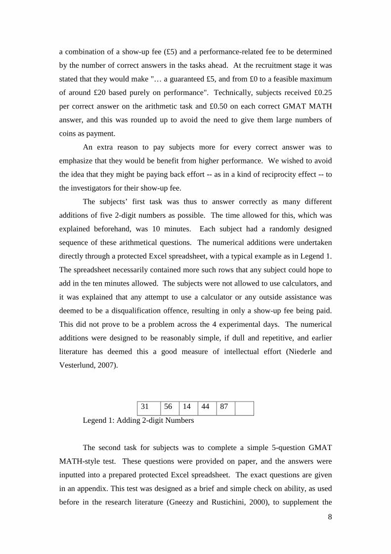
sequence of these arithmetical questions. The numerical additions were undertaken

directly through a protected Excel spreadsheet, with a typical example as in Legend 1.

The spreadsheet necessarily contained more such rows that any subject could hope to

add in the ten minutes allowed. The subjects were not allowed to use calculators, and

it was explained that any attempt to use a calculator or any outside assistance was

deemed to be a disqualification offence, resulting in only a show-up fee being paid.

This did not prove to be a problem across the 4 experimental days. The numerical

additions were designed to be reasonably simple, if dull and repetitive, and earlier

literature has deemed this a good measure of intellectual effort (Niederle and

Vesterlund, 2007).

31 56 14 44 87

Legend 1: Adding 2-digit Numbers

The second task for subjects was to complete a simple 5-question GMAT

MATH-style test. These questions were provided on paper, and the answers were

inputted into a prepared protected Excel spreadsheet. The exact questions are given

in an appendix. This test was designed as a brief and simple check on ability, as used

before in the research literature (Gneezy and Rustichini, 2000), to supplement the

9

questionnaire.

The final task, which was not subject to a performance-related payment (and

subjects were made aware of this), was to complete a questionnaire. A copy of this is

provided in the appendix. The questionnaire inquired into both the happiness level of

subjects (before and after the clip for treatment 1), and their level of mathematical

expertise. The wording was designed to be simple to answer; anonymity was once

again stressed before it was undertaken; the scale used was a conventional 7-point

metric, following the well-being literature.

To summarize the timeline:3

1. Subjects enter and are given basic instructions on experimental

etiquette.

2. Subjects in treatment 1 are exposed to a comedy clip for 10

minutes, otherwise not.

3. Subjects are given additional instructions, including a statement

that their final payment relates to the number of correct answers, and

instructed against the use of calculators or similar.

4. Subjects move to their networked consoles and undertake the

numerical additions for 10 minutes.

5. Results are saved and a new task is initiated, with subjects

undertaking the GMAT MATH-style test for 5 minutes.

6. Results are again saved, and subjects then complete the final

questionnaire.

7. After the questionnaire has been completed, subjects receive

payment as calculated by the central computer.

Results

A group of 182 subjects drawn from the University of Warwick participated in

the experiment, each taking part in only one session. A breakdown of the numbers

per day and session follows. As explained in Table 1, the subject pool was made up

of 100 males and 73 females. Table 2 summarizes the means and standard deviations

of main variables. The first variable is the number of correct additions in the allotted

ten minutes. ‘Happiness before’ is the self reported level of happiness (for the treated

3 The full instructions provided in the appendix provide a description of the timing.

10

group before the clip) on a seven point scale. The variable ‘happiness after’ is the

level of happiness after the clip for the treated group; GMAT MATH is the number of

correct problem solved; Mathematical qualification is an index calculated from the

questionnaire. Enjoyment-of-clip is a measure in a range between 1 and 7 of level of

how much they liked the movie clip.

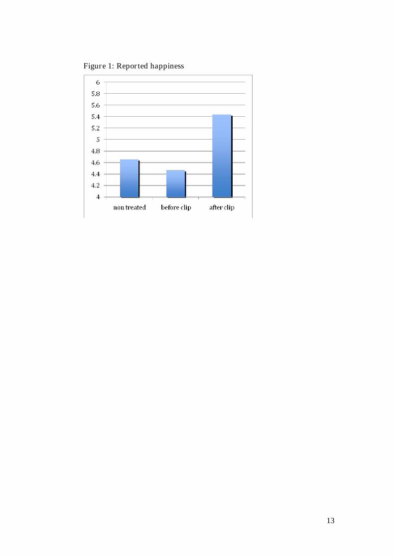
According to the data, the clip is successful in increasing the happiness levels

of subjects. As shown in Figure 1, they report an average rise of almost one point

(0.98) on the scale of 1 to 7. Comparing the ex-post happiness of the treated subject

with that of the non-treated subjects, we observe that the average of the former is

higher by 0.85 points. Using a two-sided t-test, this difference is statistically

significant (p <0.01). Finally, it is useful to notice that the level of happiness before

the clip for the treated group is not statistically significantly different (the difference

is just 0.13) from the happiness of the untreated group (p = 0.20 on the difference).

In Figure 2 we display the average productivity in the test. The treated group’s

mean performance is higher by 1.71 additions than the average performance of the

untreated group. This difference is approximately ten percent. It is statistically

significantly different from zero (p=0.04).

Interestingly, and perhaps encouragingly, the performance of those 16 subjects

in the treated group who did not report an increase in happiness is statistically non

different from the performance of the untreated group (p=0.67). Therefore, the

increase in the performance seems to be linked to the increase in happiness rather than

merely to the fact of watching the clip. The clip did not hamper the performance of

subjects who did not declare themselves happier.4 For them, the effect is zero.

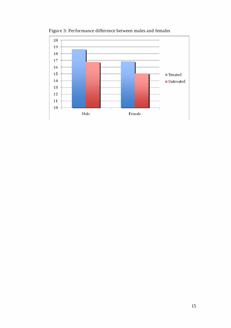
In Figure 3 we show the performances of male and female subjects. Both

groups feature a similar increase in their performances (1.9 for male, 1.78 for female).

From the cumulative distributions for the number of correct answers for the

treated and untreated group, shown in Figure 4, we see that the treatment increase the

performances of low and medium performers, while the high performers are less

affected.

We also performed OLS-based regressions to analyze the determinants of the

performances.

Table 3 presents the determinants of the number of correct additions; variable

4 Also, the 17 subjects who did not declare an increase in happiness enjoyed the clip. In a range of values between 1 and 7, theaverage is 5.41, with a minimum of 5 and a maximum of 7.

11

Change-in-Happiness is the difference in happiness before and after the clip; Math-

qualification is a measure of knowledge in mathematics determined by past studies.

Day 2, Day 3 and Day 4 are day dummies. GMAT MATH is a test score that records

the subjects’ intellectual skills.

Consistent with the result seen in the previous session, the subjects’

performances are higher in the session with treatment. As we can see in regression

(1), this results hold when we control for subjects’ characteristics and periods. In

regression (2) we show that the performances are more generally increasing with the

increase of elicited happiness (for the case of untreated subjects, by definition,

Change-in-Happiness=0). This result is still true when we restrict the analysis to the

treated subjects like in regression (3).

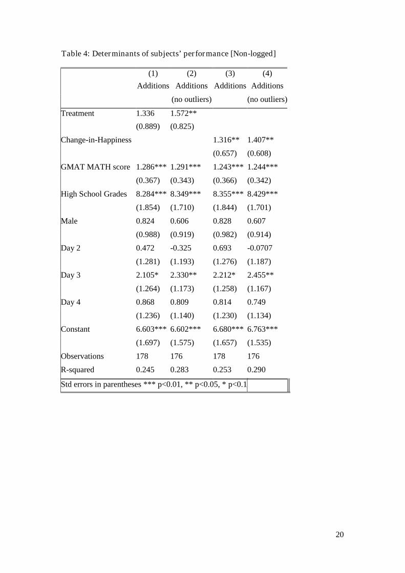
As a check, Table 4 re-runs the first two regressions of Table 3 with absolute

values rather than log values. The variable ‘Treatment’ is positive and significant

when, as in regression 2, we exclude the outliers (we drop the observations with 2 and

43 correct additions). The variable Change-in-Happiness is significant irrespective of

whether or not we keep in the two outliers (regressions 3 and 4).

It seems that positive emotion invigorates people. Yet the mechanism here, so

far, is unclear. Does happiness have its effect through greater numbers answered or

through greater accuracy of the average answer? The distinction is of interest and

might be thought of as one between industry and talent --between the consequences of

happiness for pure effort compared to effective skill.

To inquire into this, we estimate different kinds of equations.

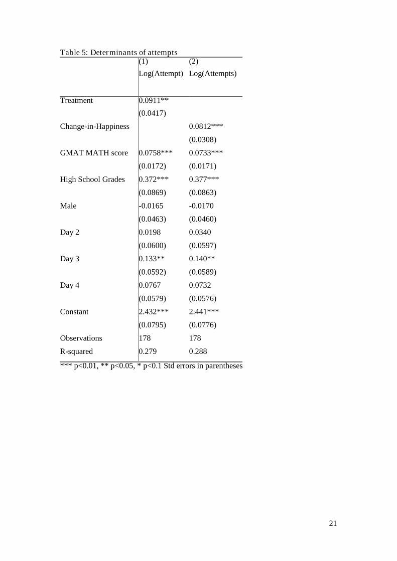
Table 5 takes attempted additions (in log terms) as the dependent variable. The

results are similar to the ones in Table 3, where we considered the # of correct

additions. Then, in Table 6, we run exactly the same regression as in Table 5 but with

the different dependent variable. This is an estimated equation for the ratio of correct-

answers to attempted-answers. Interestingly, neither the dummy treatment nor

Change-in-Happiness is statistically significantly different from zero. Therefore, the

treatment acts as an intercept shifter in the attempts equation rather than in extra

precision. It is also worth noticing that the precision results are influenced by the

underlyling mathematical skill, as measured by the mini GMAT MATH score, and to

a lesser extent by mathematical knowledge.

Standing back from the details, there seem to be a number of implications

from the experiment. First, economics may need to pay more attention to what

12

emotions do. In so far as they play a role at all in economics, they have been viewed,

as in the happiness literature, as something to be treated as a dependent variable.

Second, it seems clear that better bridges should be built between applied psychology

and the discipline of economics. Third, if happiness boosts productivity, this raises

the possibility of virtual spirals -- that might even operate at the macroeconomic level.

Happiness might lead to greater productivity which might in turn lead to greater

happiness.

Conclusions

Little is known by economists about how emotions affect productivity. To try

to make progress on this, we design a randomized trial, and thus are able exogenously

to ‘assign’ different emotions to different people. Some of our laboratory subjects

have their happiness levels increased. Some, in a control group, do not. A rise in

happiness seems to lead to greater productivity in a paid piece-rate task. The effect is

large, can be replicated, exists in male and female subsamples, and is not plausibly a

reciprocity effect.

13

Figure 1: Reported happiness

14

Figure 2: Number of correct additions

15

Figure 3: Performance difference between males and females

16

Figure 4: CDF of subjects’ performances

0.2

.4.6

.81

0 10 20 30 40Correct Additions

CDF Treated CDF Untreated

17

Table 1: Subject numbers for each session and day

Day Treated Untreated

1 24 24

2 23 20

3 23 24

4 24 25

18

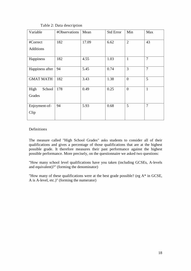
Table 2: Data description

Variable #Observations Mean Std Error Min Max

#Correct

Additions

182 17.09 6.62 2 43

Happiness 182 4.55 1.03 1 7

Happiness after 94 5.45 0.74 3 7

GMAT MATH 182 3.43 1.38 0 5

High School

Grades

178 0.49 0.25 0 1

Enjoyment-of-

Clip

94 5.93 0.68 5 7

Definitions

The measure called "High School Grades" asks students to consider all of theirqualifications and gives a percentage of those qualifications that are at the highestpossible grade. It therefore measures their past performance against the highestpossible performance. More precisely, on the questionnaire we asked two questions:

"How many school level qualifications have you taken (including GCSEs, A-levelsand equivalent)?" (forming the denominator)

"How many of these qualifications were at the best grade possible? (eg A* in GCSE,A is A-level, etc.)" (forming the numerator)

19

Table 3: Determinants of subjects’ performance5

(1) (2) (3)

log(Additions)log(Additions)log(Additions)

Treated only

Treatment 0.118**

(0.0548)

Change-in-Happiness 0.101** 0.0847*

(0.0405) (0.0495)

GMAT MATH score 0.104*** 0.100*** 0.0739***

(0.0226) (0.0226) (0.0273)

High School Grades 0.471*** 0.477*** 0.428***

(0.114) (0.114) (0.124)

Male -0.0257 -0.0267 0.00675

(0.0609) (0.0606) (0.0774)

Day 2 -0.0169 0.000901 -0.0170

(0.0790) (0.0787) (0.0905)

Day 3 0.0975 0.106 0.131

(0.0779) (0.0776) (0.0885)

Day 4 0.0118 0.00724 -0.00752

(0.0762) (0.0758) (0.0895)

Constant 2.106*** 2.120*** 2.244***

(0.105) (0.102) (0.126)

Observations 178 178 93

R-squared 0.273 0.280 0.307

Std errors in parentheses *** p<0.01, ** p<0.05, * p<0.1

5 Within the table as is standard the notation *** indicates p<0.01, ** p<0.05, * p<0.1, and standard errors are given inparentheses.

20

Table 4: Determinants of subjects’ performance [Non-logged]

(1) (2) (3) (4)

Additions Additions Additions Additions

(no outliers) (no outliers)

Treatment 1.336 1.572**

(0.889) (0.825)

Change-in-Happiness 1.316** 1.407**

(0.657) (0.608)

GMAT MATH score 1.286*** 1.291*** 1.243*** 1.244***

(0.367) (0.343) (0.366) (0.342)

High School Grades 8.284*** 8.349*** 8.355*** 8.429***

(1.854) (1.710) (1.844) (1.701)

Male 0.824 0.606 0.828 0.607

(0.988) (0.919) (0.982) (0.914)

Day 2 0.472 -0.325 0.693 -0.0707

(1.281) (1.193) (1.276) (1.187)

Day 3 2.105* 2.330** 2.212* 2.455**

(1.264) (1.173) (1.258) (1.167)

Day 4 0.868 0.809 0.814 0.749

(1.236) (1.140) (1.230) (1.134)

Constant 6.603*** 6.602*** 6.680*** 6.763***

(1.697) (1.575) (1.657) (1.535)

Observations 178 176 178 176

R-squared 0.245 0.283 0.253 0.290

Std errors in parentheses *** p<0.01, ** p<0.05, * p<0.1

21

Table 5: Determinants of attempts(1) (2)

Log(Attempt) Log(Attempts)

Treatment 0.0911**

(0.0417)

Change-in-Happiness 0.0812***

(0.0308)

GMAT MATH score 0.0758*** 0.0733***

(0.0172) (0.0171)

High School Grades 0.372*** 0.377***

(0.0869) (0.0863)

Male -0.0165 -0.0170

(0.0463) (0.0460)

Day 2 0.0198 0.0340

(0.0600) (0.0597)

Day 3 0.133** 0.140**

(0.0592) (0.0589)

Day 4 0.0767 0.0732

(0.0579) (0.0576)

Constant 2.432*** 2.441***

(0.0795) (0.0776)

Observations 178 178

R-squared 0.279 0.288

*** p<0.01, ** p<0.05, * p<0.1 Std errors in parentheses

22

Table 6: Determinants of the precision

(ie. ratio of correct answers)

(1) (2)

Correct/ Correct/

Attempt Attempt

Treatment 0.0128

(0.0185)

Change-in-Happiness 0.0102

(0.0138)

GMAT MATH score 0.0165** 0.0162**

(0.00765)(0.00767)

High School Grades 0.0656* 0.0663*

(0.0386) (0.0386)

Male 0.00152 0.00134

(0.0206) (0.0206)

Day 2 -0.0268 -0.0249

(0.0267) (0.0267)

Day 3 -0.0201 -0.0192

(0.0263) (0.0263)

Day 4 -0.0507* -0.0512**

(0.0258) (0.0257)

Constant 0.753*** 0.755***

(0.0354) (0.0347)

Observations 178 178

R-squared 0.095 0.096

Std. errors in parentheses *** p<0.01,

** p<0.05, * p<0.1

23

References

Amabile, T.M., Barsade, S.G., Mueller, J.S., Staw, B.M. 2005. Affect and creativityat work. Administrative Science Quarterly 50, 367-403.

Argyle, M., 1989. The Psychology of Happiness. London: Routledge

Argyle, M., 1989. Do happy workers work harder? The effect of job satisfaction onjob performance. In: Ruut Veenhoven (ed), (1989) How harmful is happiness?Consequences of enjoying life or not, Universitaire Pers Rotterdam, TheNetherlands.

Ashby, F.G., Isen, A.M.,Turken, A.U. A neuropsychological theory of positive affectand its influence on cognition. Psychological Review 106, 529-550.

Blanchflower, D.G., Oswald, A.J., 2004. Well-being over time in Britain and theUSA. Journal of Public Economics 88, 1359-1386.

Boehm, J.K., Lyubomirsky, S. 2008. Does happiness promote career success? Journalof Career Assessment 16, 101-116.

Brickman, P., Coates, D., Janoff-Bulman, R., 1978. Lottery winners and accidentvictims – is happiness relative? Journal of Personality and Social Psychology36, 917-927.

Clark, A.E., 1999. Are wages habit-forming? Evidence from micro data, Journal ofEconomic Behavior and Organization 39, 179-200.

Clark, A. E., Diener, E., Georgellis, Y., Lucas, R. E., 2008. Lags and leads in lifesatisfaction: A test of the baseline hypothesis. Economic Journal 118: F222-F243.

Clark, A.E., Oswald, A.J., 1994. Unhappiness and unemployment. Economic Journal104, 648-659.

Clark, A.E., Oswald, A.J., 2002. A simple statistical method for measuring how lifeevents affect happiness. International Journal of Epidemiology 31, 1139-1144.

Diener, E., Suh, E.M., Lucas, R.E., Smith, H.L., 1999. Subjective well-being: Threedecades of progress. Psychological Bulletin 125(2), 276-302.

Di Tella, R., MacCulloch, R.J., Oswald, A.J., 2001. Preferences over inflation andunemployment: Evidence from surveys of happiness. American EconomicReview 91, 335-341.

Di Tella, R., MacCulloch, R.J., Oswald, A.J., 2003. The macroeconomics ofhappiness. Review of Economics and Statistics 85, 809-827.

Di Tella, R., Haisken, J., Macculloch, R., 2005. Happiness adaptation to income andto status in an individual panel, working paper, Harvard Business School.

Easterlin, R.A., 2001. Income and happiness: Towards a unified theory. EconomicJournal 111, 465-484.

24

Easterlin, R.A., 2003. Explaining happiness. Proceedings of the National Academy ofSciences 100, 11176-11183.

Easterlin, R.A., 2005. A puzzle for adaptive theory. Journal of Economic Behaviorand Organization 56, 513-521.

Elster, J. 1998. Emotions and economic theory. Journal of Economic Literature, 36,47–74.

Erez, A., Isen, A. M. 2002 The influence of positive affect on the components ofexpectancy motivation. Journal of Applied Psychology, 87, 1055–1067.

Ferrer-i-Carbonell A., 2005. Income and well-being: An empirical analysis of thecomparison income effect. Journal of Public Economics 89, 997-1019.

Ferrer-i-Carbonell A., Van Praag B.M.S., 2002. The subjective costs of health lossesdue to chronic diseases. An alternative model for monetary appraisal. HealthEconomics 11, 709-722.

Frank, R. H. 1988. Passions within reason. New York: Norton.

Fredrickson, B. L., Joiner, T., 2002. Positive emotions trigger upward spirals towardemotional well-being. Psychological Science, 13, 172–175.

Frey, B.S., Meier, S., 2004. Social comparisons and pro-social behaviour: Testingconditional cooperation in a field experiment. American Economic Review94(5), 1717-1722.

Frey, B. S., Stutzer, A., 2002. Happiness and Economics. Princeton, USA.

Frey, B.S., Stutzer, A., 2006. Does marriage make people happy, or do happy peopleget married? Journal of Socio-economics, 35, 326-347.

Gilbert, D. T., Pinel, E. C., Wilson, T. D., Blumberg, S. J., Wheatley, T., 1998.Immune neglect: A source of durability bias in affective forecasting. Journal ofPersonality and Social Psychology 75, 617-638.

Gneezy, U. and Rustichini, A., 2000, “Pay enough or don't pay at all”, QuarterlyJournal of Economics Vol. 115, No. 3, 791-810.

Groot, W., Van den Brink, M., 2000, Life-satisfaction and preference drift. SocialIndicators Research 50, 315-328.

Groot, W., van den Brink, H.T.M., Plug, E., 2004. Money for health: the equivalentvariation of cardiovascular diseases. Health Economics 13, 859-872.

Hermalin, B.E., Isen, A.M., 2008. A model of the effect of affect on economicdecision-making. Quantitative Marketing and Economics 6, 17-40.

Isen, A.M. 1987. Positive affect, cognitive processes, and social behaviour. Advancesin Experimental Social Psychology 20, 203-253.

Isen, A.M., Daubman, K.A., Nowicki, G.P., 1987. Positive affect facilitates creativeproblem-solving. Journal of Personality and Social Psychology 52, 1122-1131.

25

Isen, A. M. 2000. Positive affect and decision making. In M. Lewis & J. M. Haviland(Eds.), Handbook of emotions. 2nd ed. New York: The Guilford Press.

Isen, A. M., Reeve, J., 2005. The influence of positive affect on intrinsic andextrinisic motivation: Facilitating enjoyment of play, responsible work behavior,and self-control. Motivation and Emotion, 29, 297–325.

Isen, A. M., Nygren, T. E., Gregory Ashby, F., 1988. Influence of positive affect onthe subjective utility of gains and losses; It is just not worth the risk. Journal ofPersonality and Social Psychology, 55, 710–717.

Kahneman, D., Sugden, R., 2005. Experienced utility as a standard of policyevaluation. Environmental and Resource Economics 32, 161-181.

Layard, R., 2005. Happiness: Lessons from a New Science, Allen Lane, London.

Loewenstein, G. 1996. Out of control: Visceral influences on behavior.Organizational Behavior and Human Decision Processes, 65, 272–292.

Loewenstein, G. 2000. Emotions in economic theory and economic behavior.American Economic Review, 90, 426–432.

Loewenstein, G., O’Donaghue, T. 2004. Animal spirits: Affective and deliberativeprocesses in economic behavior, working paper.

Loomes, G., Sugden, R. 1982. Regret theory: An alternative theory of rational choiceunder uncertainty. Economic Journal, 92, 805–824.

Luttmer, E.F.P., 2005. Neighbors as negatives: Relative earnings and well-being.Quarterly Journal of Economics 120, 963-1002.

Lyubomirsky, S., King, L., Diener, E., 2005. The benefits of frequent positive affect:Does happiness lead to success? Psychological Bulletin, 131, 803-855.

Lyubomirsky, S., Sheldon, K.M., Schkade, D., 2005. Pursuing happiness: Thearchitecture of sustainable change. Review of General Psychology 9, 111-131.

Niederle, M. and Vesterlund, L., 2007. Do women shy away from competition? Domen compete too much?. Quarterly Journal of Economics 122.

Oswald, A.J., 1997. Happiness and economic performance. Economic Journal 107,1815-1831.

Oswald, A.J., Powdthavee, N., 2005. Does happiness adapt? A longitudinal study ofdisability with implications for economists and judges. Working paper,Warwick University (also available as IZA working paper #2208, 2006).

Oswald, A.J., Powdthavee, N., 2008. Death, happiness, and the calculation ofcompensatory damages. Journal of Legal Studies, forthcoming.

Patterson, M., Warr, P., West, M. 2004. Organizational climate and companyproductivity: The role of employee affect and employee level. Journal ofOccupational and Organizational Psychology, 77, 193-216.

26

Posner, E. A., 2000. Law and the emotions. University of Chicago Law & Economics,Olin Working Paper No. 103.

Posner, E.A., Sunstein, C.R., 2005. Dollars and death. University of Chicago LawReview 72, 537-598.

Sanna, L.J., Turley, K.J., Mark, M.M., 1996. Expected evaluation, goals, andperformance: Mood as input. Personality and Social Psychology Bulletin 22,323-325.

Senik, C., 2004. When information dominates comparison – Learning from Russiansubjective panel data. Journal of Public Economics 88, 2099-2123.

Smith, D.M., Langa, K.M., Kabeto, M.U., Ubel, P.A., 2005. Health, wealth andhappiness. Psychological Science 16, 663-666.

Stutzer, A. 2004., The role of income aspirations in individual happiness. Journal ofEconomic Behavior and Organization 54, 89-109.

Tsai, W-C., Chen, C-C., Liu, H-L., 2007, Test of a model linking employee positivemoods and task performance. Journal of Applied Psychology, 92, 1570-1583.

Van Praag, B., Ferrer-I-Carbonell, A., 2004. Happiness Quantified: A SatisfactionCalculus Approach, Oxford University Press, Oxford.

Westermann, R., Spies, K., Stahl, G., and Hesses, F. W., 1996, “Relativeeffectiveness and validity of mood induction procedures: a metaanalysis”,European Journal of Social Psychology Vol. 26, 557-580

Winkelmann, L., Winkelmann, R., 1998. Why are the unemployed so unhappy?Evidence from panel data. Economica 65, 1-15.

Wright, T.A., Staw, B.A. 1999. Affect and favorable work outcomes: two longitudinaltests of the happy-productive worker thesis. Journal of OrganizationalBehavior, 20, 1-23.

Wu S., 2001. Adapting to heart conditions: a test of the hedonic treadmill. Journal ofHealth Economics 20, 495-508.

Zimmermann, A., Easterlin, R.A., 2006. Happily ever after? Cohabitation, marriage,divorce, and happiness in Germany. Population and Development Review 32,511 – 528.

27

APPENDIX FOR PARIS TALK

Replication of findings

The experiment was carried out on four separate days, as follows:

Session Treatment Date Time

1 Treatment 0 21 May 2008 2.30-3.30pm

1 Treatment 1 21 May 2008 4.00-5.00pm

2 Treatment 0 18 June 2008 2.30-3.30pm

2 Treatment 1 18 June 2008 4.00-5.00pm

3 Treatment 1 10 October 2008 2.30-3.30pm




Table 1: Treatment Dates

Recall that treatment 0 is the treatment without a video clip and treatment 1 includes

a video clip. Sessions 1 and 2 were undertaken in term 3 of the University of Warwick

academic year 2007-8, while sessions 3 and 4 were undertaken in term 1 of the 2008-9

academic year. Since they are separated by a gap of approximately 4 months, we might wish

to check for significant changes across the time between sessions 1-2 and sessions 3-4. The

key aggregate variables results broken down by session are as follows:

Session addscore log

addscore

Addscore

Male

Addscore

Female

happy

before

happy

after

enjoy

clip

1 Treatment 0 15.38** 1.17 14.88** 16.83 4.54 na na

1 Treatment 1 18.21** 1.23 18.26** 18 4.54 5.63 5.96

2 Treatment 0 16.85 1.18 19.41 13* 4.45 na na

2 Treatment 1 16.48 1.19 16.36 16.58* 4.43 5.22 5.74

3 Treatment 0 16.26* 1.16 15.75* 17.14 4.79 na na

3 Treatment 1 19.52* 1.27 20.42* 18.11 4.48 5.39 5.83

4 Treatment 0 16.04 1.15 18.07 14.36 4.92 na na

4 Treatment 1 17.72 1.22 19.6 15.92 4.36 5.44 6.21

Table 2: Summary Statistics by Treatment

The key column is perhaps log addscore (log correct additions) which smoothes for

outliers in the number of correctly answered numerical additions within 10 minutes. As can

be seen from the table, the data for sessions 1-2 are very similar to those from sessions 3-4. In

particular the happiness levels are similar, and the clip seems to have induced similar increase

across all sessions. Most importantly, the pattern of results seems consistent across all four

sessions. The only exception comes in session 2 where the raw number of additions does not

rise moving from treatment 0 to treatment 1. This is entirely down to one outlier who

performed extremely well in treatment 0, and using logs to mute the impact of outliers brings

28

the results into alignment with the other sessions.6

Note that we put an asterisk when the difference between treated and untreated

groups are statistically significant, using a simple ttest. In particular we have that for session 1

(21 May 2008) and 3 (10 October 2008) the difference for the entire pool is already

statistically significant with a p-values 0.047 and 0.052 respectively. When we split the

group in male and female we note that they are already statistically significant in 3 out of 8

subcases. Of course summing all four the significance rises as indicated in the main text.

Alternatively we also regressed the key variables for all four sessions individually as

below:

(1) (2) (3) (4) (5) (6) (7) (8)VARIABLES ladd ladd ladd ladd ladd ladd ladd ladd

treatment 0.129 0.0931 0.184 0.0979(0.0889) (0.124) (0.127) (0.118)

gmatscore 0.0799* 0.0859* 0.115** 0.110** 0.139*** 0.135*** 0.0739 0.0722(0.0472) (0.0453) (0.0507) (0.0510) (0.0434) (0.0448) (0.0473) (0.0469)

qualifs 0.482** 0.486** 0.398 0.386 0.277 0.332 0.657*** 0.652***(0.198) (0.192) (0.261) (0.266) (0.262) (0.262) (0.239) (0.236)

male -0.0729 -0.0373 0.113 0.0985 -0.153 -0.150 -0.0258 -0.0350(0.111) (0.110) (0.127) (0.126) (0.134) (0.136) (0.136) (0.133)

dhappy 0.126** 0.0256 0.0993 0.0980(0.0585) (0.112) (0.102) (0.0792)

Constant 2.220*** 2.165*** 2.022*** 2.093*** 2.219*** 2.256*** 2.122*** 2.128***(0.187) (0.185) (0.218) (0.198) (0.184) (0.184) (0.170) (0.163)

Observations 48 48 40 40 41 41 49 49R-squared 0.286 0.323 0.288 0.278 0.336 0.315 0.264 0.278

Notes: *** p<0.01, ** p<0.05, * p<0.1. Standard errors in parentheses

Table 3: Session regressions

Regression (1) considers log addscore from session 1 regressed on treatment, with (2)

instead using dhappy. Dhappy is in general a better measure of the impact of happiness since

it controls for those subjects who did not gain in happiness from watching the clip. (3) and (4)

are the respective regressions for session 2, (5) and (6) forsession 3 and (7) and (8) for session

4. We might also consider merging sessions 1 and 2, and merging sessions 3 and 4 as below.

(1) (2) (3) (4)VARIABLES ladd ladd ladd ladd

treatment 0.0989 0.139(0.0712) (0.0848)

gmatscore 0.100*** 0.0987*** 0.111*** 0.108***(0.0333) (0.0330) (0.0316) (0.0318)

qualifs 0.458*** 0.462*** 0.468*** 0.479***(0.157) (0.155) (0.169) (0.169)

male 0.0299 0.0309 -0.0658 -0.0720(0.0797) (0.0789) (0.0918) (0.0916)

dhappy 0.0990* 0.0982(0.0535) (0.0617)

Constant 2.091*** 2.096*** 2.147*** 2.174***(0.135) (0.130) (0.122) (0.118)

Observations 88 88 90 90R-squared 0.268 0.281 0.274 0.273

Notes: *** p<0.01, ** p<0.05, * p<0.1. Standard errors in parentheses

Table 4: Grouped session regressions

6 6 Without the outlier who performed 43 exact additions, the average is 16.47 in treated and 16.47 inthe untreated group.

29

In table 4 regression (1) and (2) group sessions 1 and 2, while regression (3) and (4)

group sessions 3 and 4. As in table 3, the first regression in each pair considers treatment

while the

30

Appendix

The appendix includes a full set of subject instructions (Appendix A), a copy of the

GMAT MATH-style test (Appendix B) and the questionnaire (Appendix C).

Appendix A: Instructions

[bold = only for the clip treatment, X talks directly with subjects, Y, Z, etc. are

assistants. Parts in square brackets are not to read out.]

[X invites subjects to enter room while Y sets up the video clip]

Welcome to the session. My name is X, and working with me today are Y, Z, etc.

Many thanks for attending today. You will be asked to perform a small number of very minor

tasks and will be paid both a show-up fee and an amount based on how you perform, but first

we would like to ask you to watch a video clip. Please do not talk to each other at any stage

in the session. If you have any questions please raise your hands, but avoid distracting the

others in the room.

Z will now guide you to the seats at the front of the room directly in front of the

projector, while Y prepares the video clip. Please make yourselves comfortable: the clip

will last about 10 minutes and I will have more instructions for you afterwards.

[10 minutes: video clip]

Thanks for watching. Z will now distribute ID cards to you and you are asked to sit

at the computer corresponding to the ID number. Everything is done anonymously – your

performance will simply be recorded based on the ID card, and not your names. You will find

some paper and a pen next to your computer – use them if you wish, and raise your hand if

you wish to request additional paper. Please do not use calculators or attempt to do anything

other than answer the questions through mental arithmetic. If we observe any form of

cheating it will invalidate your answers and you will be disqualified, and therefore receive

only the show-up fee.

For the first task you will have 10 minutes to add a sequence of numbers together and

enter your answers in the column labelled “answer”. To remind you, you will be paid based

on the number of correct answers that you produce. When the ten minutes are over I will ask

you to stop what you are doing and your results will be saved.

Next look at your screens: you will find that a file called “Numberadditions.xls” is

open but minimized on your screen. Please now maximize the file by clicking on the tab. You

have ten minutes starting now.

[10 minutes: number additions]

31

Please stop what you are doing, your answers will now be saved. Y and Z will now

visit your computers and place a sheet faced down next to your keyboards. Please do not turn

over the sheet until I ask.

[Y and Z move to terminals, placing question sheets faced down]

For the second task we would like you answer a small number of questions. You can

maximise the file on your computer labelled “GMAT MATH.xls” and you will once again

see a column labelled answers. In this column you will have to enter a letter from (a) to (e),

corresponding to a multiple-choice answer to the sheet which is faced-down in front of you.

Once again, I remind you that you will be paid based on the number of correct answers. You

have 5 minutes to attempt these questions, please turn over the sheets and begin.

[5 minutes: GMAT MATH-style test ]

Please stop what you are doing, your answers will now be saved. You should next

open the final document: a questionnaire that you are asked to complete. You will be given 10

minutes to complete this, though if you need additional time we can extend this deadline

indefinitely. Please answer as truthfully as you can and feel free to raise your hands if

anything is unclear. To stress, where you are asked to input a number from 1 to 7, “7” is the

high number and “1” is the low one.

[10 minutes: questionnaire]

Hopefully you have all had a chance to complete the questionnaire. If you need more

time, then please raise your hand. Otherwise we will save your questionnaire replies.

The central computer has calculated your payments. Please remain at your computer

for the time being. I will ask you to approach the front in order of your ID numbers and you

will need to sign a receipt for your payments and to hand in both your ID cards and the test

document before receiving payment. Many thanks for taking part in today’s session.

[Test documents destroyed, ID cards collected, receipts signed and payments handed

out]

Appendix B: GMAT MATH-style Test

Questions

Please answer these by inserting the multiple choice answer a, b, c, d or e into the

GMAT MATH spreadsheet on your computer.

32

1. Harriet wants to put up fencing around three sides of her rectangular yard and leave

a side of 20 feet unfenced. If the yard has an area of 680 square feet, how many feet of

fencing does she need?

a) 34

b) 40

c) 68

d) 88

e) 102

2. If x + 5y = 16 and x = -3y, then y =

a) -24

b) -8

c) -2

d) 2

e) 8

3. If “basis points” are defined so that 1 percent is equal to 100 basis points, then 82.5

percent is how many basis points greater than 62.5 percent?

a) .02

b) .2

c) 20

d) 200

e) 2,000

4. Which of the following best completes the passage below?

In a survey of job applicants, two-fifths admitted to being at least a little dishonest.

However, the survey may underestimate the proportion of job applicants who are dishonest,

because—–.

a) some dishonest people taking the survey might have claimed on the survey to be

honest.

b) some generally honest people taking the survey might have claimed on the survey

to be dishonest.

33

c) some people who claimed on the survey to be at least a little dishonest may be very

dishonest.

d) some people who claimed on the survey to be dishonest may have been answering

honestly.

e) some people who are not job applicants are probably at least a little dishonest.

5.People buy prestige when they buy a premium product. They want to be associated

with something special. Mass-marketing techniques and price-reduction strategies should not

be used because —–.

a) affluent purchasers currently represent a shrinking portion of the population of all

purchasers.

b) continued sales depend directly on the maintenance of an aura of exclusivity.

c) purchasers of premium products are concerned with the quality as well as with the

price of the products.

d) expansion of the market niche to include a broader spectrum of consumers will

increase profits.

e) manufacturing a premium brand is not necessarily more costly than manufacturing

a standard brand of the same product.

34

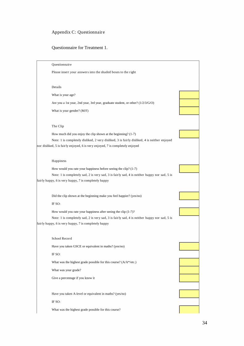
Appendix C: Questionnaire

Questionnaire for Treatment 1.

Questionnaire

Please insert your answers into the shaded boxes to the right

Details

What is your age?

Are you a 1st year, 2nd year, 3rd year, graduate student, or other? (1/2/3/G/O)

What is your gender? (M/F)

The Clip

How much did you enjoy the clip shown at the beginning? (1-7)

Note: 1 is completely disliked, 2 very disliked, 3 is fairly disliked, 4 is neither enjoyed

nor disliked, 5 is fairly enjoyed, 6 is very enjoyed, 7 is completely enjoyed

Happiness

How would you rate your happiness before seeing the clip? (1-7)

Note: 1 is completely sad, 2 is very sad, 3 is fairly sad, 4 is neither happy nor sad, 5 is

fairly happy, 6 is very happy, 7 is completely happy

Did the clip shown at the beginning make you feel happier? (yes/no)

IF SO:

How would you rate your happiness after seeing the clip (1-7)?



School Record

Have you taken GSCE or equivalent in maths? (yes/no)

IF SO:

What was the highest grade possible for this course? (A/A*/etc.)

What was your grade?

Give a percentage if you know it

Have you taken A-level or equivalent in maths? (yes/no)

IF SO:

What was the highest grade possible for this course?

35



How many school level qualifications have you taken (including GCSEs, A-levels and

equivalent)?

How many of these qualifications were at the best grade possible? (eg A* in GCSE, A is

A-level, etc.)

University Record

Are you currently or have you ever been a student (yes/no)

If yes, which degree course(s)?

IF you are a second or third year student what class best describes your overall

performance to date? (1/2.1/2.2/3/Fail)

36

Questionnaire for Treatment 0.

Questionnaire

Please insert your answers into the shaded boxes to the right

Details

What is your age?

Are you a 1st year, 2nd year, 3rd year, graduate student, or other? (1/2/3/G/O)

What is your gender? (M/F)

Happiness

How would you rate your happiness at the moment? (1-7)



School Record

Have you taken GSCE or equivalent in maths? (yes/no)

IF SO:

What was the highest grade possible for this course? (A/A*/etc.)



Have you taken A-level or equivalent in maths? (yes/no)

IF SO:

What was the highest grade possible for this course?



How many school level qualifications have you taken (including GCSEs, A-levels and

equivalent)?

How many of these qualifications were at the best grade possible? (eg A* in GCSE, A is A-

level, etc.)

University Record

Are you currently or have you ever been a student (yes/no)

If yes, which degree course(s)?

IF you are a second or third year student what class best describes your overall performance to

date? (1/2.1/2.2/3/Fail)

happiness and productivity - École normale...

Documents