Growth and Welfare Effects of Business Cycles In

Economies with Idiosyncratic Human Capital Risk

First Version: September, 2001

This Draft: October, 2002

Tom Krebs∗

Brown University†

Abstract

This paper uses a tractable macroeconomic model with idiosyncratic human capital risk and incompletemarkets to analyze the growth and welfare effects of business cycles. The analysis is based on the assumptionthat the elimination of business cycles eliminates the variation in idiosyncratic risk. The paper shows that areduction in the variation in idiosyncratic risk decreases the ratio of physical to human capital and increasesthe total investment return and welfare. If the degree of risk aversion is less than or equal to one, theneconomic growth is enhanced. This paper also provides a quantitative assessment of the macroeconomiceffects of business cycles based on a calibrated version of the model. Even for relatively small degrees of riskaversion (around one) the model implies that the elimination of business cycles has substantial effects oninvestment in physical and human capital, economic growth, and welfare.

JEL Classification: D52, E32, O40Keywords : Cost of Business Cycles, Growth, Idiosyncratic Risk

∗I would like to thank for helpful comments Andy Atkeson, Oded Galor, Peter Howitt, Bob Lucas, TomoNakajima, Herakles Polemarchakis, Per Krusell, Tony Smith, David Weil and seminar participants at ArizonaState University, Brown University, Carnegie-Mellon University, Columbia University, the Economic TheoryConference, Ischia 2001, the Stoney-Brook Incomplete Markets Workshop, 2001, the Minnesota Workshopin Macroeconomic Theory, 2002, and the SITE Workshop on Liquidity and Distribution in Macroeconomics,2002. Financial assistance from the Solomon Research Grant, Brown University, is gratefully acknowledged.All errors are mine.

†Current mailing address: Columbia University-GSB, Department of Finance and Economics, 3022 Broad-way, 822 Uris Hall, New York, NY 10027. E-mail: tk29@columbia.edu

I. Introduction

In a highly influential contribution, Lucas (1987) argues that the welfare costs of business

cycles are likely to be very small, and that therefore the potential benefits from counter-

cyclical stabilization policy are negligible. His argument is based on a calibrated representative-

agent model with no production, that is, Lucas (1987) assumes that there is no uninsurable

idiosyncratic risk and that economic growth and business cycles are unrelated. This pa-

per asks to what extend the introduction of market incompleteness and production changes

Lucas’ conclusions regarding the welfare cost of business cycles.

The current analysis is based on an incomplete-markets version of the class of endoge-

nous growth models analyzed by, among others, Jones and Manuelli (1990) and Rebelo

(1991).1 More specifically, households are ex ante identical and have CRRA-preferences,

production displays constant returns to scale with respect to physical and human capital,

and all markets are competitive. There are aggregate productivity shocks that affect the

return to physical and human capital investment (stock returns and wages), and there are

idiosyncratic human capital shocks that only affect human capital returns.2 Conditional on

the history of aggregate states, these idiosyncratic shocks are independently distributed over

time and identically distributed across households. Finally, the financial market structure is

incomplete in the sense that there are no assets with payoffs that depend on idiosyncratic

shocks. However, households have the opportunity to trade stocks (accumulate physical

1See also Alvarez and Stokey (1998) and Caballe and Santos (1993). Lucas (1988) analyzes a humancapital model with externalities. Krebs (2002) shows that the current incomplete-markets model admits forsimple recursive equilibria and provides a useful characterization of equilibrium, and Krebs (2001) studies aversion of the model with log-utility and no aggregate risk.

2A negative human capital shock (depreciation shocks) might occur when firm- or sector-specific skillsare either destroyed or made obsolete in the event of a job loss. Jovanovic (1979) and Ljungqvist andSargent (1998) analyze search models with specific human capital, but they assume risk-neutral workersand do not model the accumulation of physical capital. Empirically, the permanent wage loss of displacedworkers is substantial (Jacobson, LaLonde, and Sullivan 1993, Neal 1995, and Topel 1991) suggesting thatjob displacement is associated with large losses of firm or sector-specific human capital.

1

capital) and any asset (bond) in zero net supply with payoffs that depend on the aggregate

shock variable.

The incomplete-markets model analyzed in this paper is highly tractable in the sense that

there is always one equilibrium allocation that is identical to the equilibrium allocation of an

economy in which households consume and produce in autarky facing both aggregate and

idiosyncratic risk. In other words, a recursive equilibrium of the incomplete-markets economy

can be found by solving a one-agent decision problem, but this one-agent decision problem

is not the one-agent decision problem associated with the complete-markets economy (idio-

syncratic risk matters). Exploiting the tractability of the model, this paper first conducts a

qualitative analysis of the growth and welfare effects of business cycles. The analysis assumes

that the amount of idiosyncratic risk varies over the business cycle, and that the elimination

of business cycles removes these variations in idiosyncratic risk leaving the average amount

of idiosyncratic risk unchanged. The economic motivation for this assumption derives from

recent empirical work (Storesletten, Telmer, and Yaron, 2001a, and Meghir and Pistaferri,

2001) that has documented strong cyclical variations in uninsured idiosyncratic labor in-

come risk, and the notion that counter-cyclical stabilization policy might eliminate these

variations in idiosyncratic risk without changing the average amount of idiosyncratic risk

(Atkeson and Phelan, 1994, Imrohoroglu, 1989, Krusell and Smith, 1999, and Storesletten,

Telmer, and Yaron, 2001b).

The qualitative analysis shows that business cycles have the following general effects on

growth and welfare. First, a reduction in the variation in idiosyncratic human capital risk

makes human capital investment less risky, and therefore induces households to invest more

in high-return human capital. Thus, economic growth always increases if total investment in

physical and human capital does not decrease, which is the case if the degree of relative risk

aversion is less than or equal to one. However, if the degree of risk aversion is larger than

2

one, then economic growth may decrease due to the reduction in total investment. Second,

although the growth effect of eliminating business cycles might be negative for high degrees

of risk aversion, the welfare effect is always positive since the equilibrium allocation is the

solution to a one-agent decision problem.

In addition to the qualitative analysis, this paper also provides a quantitative assessment

of the growth and welfare consequences of business cycle fluctuations. The quantitative

analysis assumes that the elimination of business cycles eliminates both the fluctuations in

aggregate productivity and the variation in idiosyncratic human capital risk, and the model

economy is calibrated so that the implied variation in idiosyncratic labor income risk in the

economy with business cycles matches the estimates obtained by recent empirical studies

(Storesletten et al., 2001a, and Meghir and Pistaferri, 2001). The general finding is that

even for moderate degrees of risk aversion (around one), business cycle fluctuations have a

substantial impact on investment, growth, and welfare. In particular, the welfare gain from

eliminating business cycles is almost two orders of magnitude larger than what Lucas (1987)

has found for the complete-markets exchange economy. Most of the welfare gain is due to

the elimination of the variation in idiosyncratic human capital risk, which improves welfare

for two reasons: it eliminates the variation in the volatility of individual consumption growth

and, for moderate degrees of risk aversion, it increases average consumption growth. Both

of these welfare effects are substantial, but the volatility effect is somewhat stronger. In

short, even without an endogenous output response (exchange economy) the welfare costs

of business cycles are quite large once market incompleteness is introduced, but taking into

account the endogeneity of output (production economy) increases the cost even further.

The welfare costs of business cycles found in this paper are much larger than the welfare

costs found by Imrohoroglu (1989) and Krusell and Smith (1999), and also larger than the

costs found by Storesletten et al.(2001b). In accordance with the current analysis, all these

3

papers assume that the elimination of business cycles leads to an elimination of the variations

in idiosyncratic risk without affecting the average level of idiosyncratic risk.3 However, there

are differences in modeling the interaction between business cycles and idiosyncratic risk

that account for a substantial part of the diversion of results.

First, this paper follows Storesletten et al. (2001b) and assumes that there are permanent

idiosyncratic income shocks. In contrast, Imrohoroglu (1989) and Krusell and Smith (1999)

only consider income shocks with moderate degree of persistence, which implies that indi-

vidual consumption fluctuations are relatively small and temporary. Second, in this paper,

and to a certain extent also in Storesletten et al.(2001b), the level of aggregate economic

activity affects the magnitude of idiosyncratic income losses. Put differently, this paper as-

sumes that recessions are not only times in which the probability of job displacement goes

up, but also times in which the cost of job displacement increases. In contrast, Imrohoroglu

(1989) and Krusell and Smith (1999) assume that the level of aggregate economic activity

only affects the probability of job displacement, but not the magnitude of the income loss

experienced by displaced workers.4 As has been pointed out by Atkeson and Phelan (1994)

and Krusell and Smith (1999), in this case the elimination of business cycles only affects the

equilibrium outcome if there are indirect price effects, which are absent in the current model

and relatively small in Krusell and Smith (1999).

There is one feature of the present model that distinguishes it from all the previous

work on the welfare cost of business cycles in incomplete-market economies, namely that

3The notion that counter-cyclical stabilization policy reduces the variations in idiosyncratic risk withoutaffecting the average amount of idiosyncratic risk can be made more precise using the integration principle(Krusell and Smith, 1999) discussed in Section III. Beaudry and Page (2001) assume that the elimination ofbusiness cycles removes all uninsurable idiosyncratic risk.

4Clearly, the displacement probability increases during an economic downturn. However, there are alsogood reasons to expect the size of the income loss to be affected: the distribution of employment opportunitiesworsens inducing the unemployed worker to accept lower wage offers and to increase the average time ofsearch.

4

business cycles are detrimental to economic growth (at least for moderate degrees of risk

aversion). In contrast, the previous incomplete-markets literature has relied on a framework

that either disregards the output response to changes in business cycle activity (Imrohoroglu,

1989) or implies that the elimination of business cycles decreases output due to a reduction

in precautionary saving (Krusell and Smith, 1999, and Storesletten et al., 2001b). This

growth effect is yet another reason why the welfare cost of business cycles reported here

are substantially larger than the cost found by the previous incomplete-markets literature

(including Storesletten et al., 2001b).

This paper emphasizes the normative analysis of business cycles. However, the human

capital model with incomplete markets has also several interesting positive implications. In

particular, it provides one of the few attempts in the literature to explain formally the ob-

served negative relationship between macroeconomic volatility and economic growth (Ramey

and Ramey, 1995).5 Jones, Manuelli, and Stacchetti (1999) study this relationship within

the context of the complete-markets version of the human capital model, in which case

business cycles may affect total investment, but not the ratio of physical to human capital.

Barlevy (2000) shows that a negative relationship between aggregate volatility and economic

growth may arise in a representative-agent model with endogenous technological innovation

(Aghion and Howitt, 1992), and Acemoglu and Zilibotti (1997) discuss a model in which

non-diversifiable entrepreneurial risk affects aggregate volatility and economic growth. Fi-

nally, Boldrin and Rustichini (1994) discuss the relationship between growth and fluctuations

using a model with deterministic fundamentals and indeterminate equilibria.

5But see also Kormendi and Meguire (1985) for the opposite finding. Acemoglu and Zilibotti (1997) andQuah (1993) find a strong negative link between per capita income and volatility of growth.

5

II. Model

II.A. Economy

Consider a discrete-time infinite-horizon economy with i = 1, . . . , I households. A complete

description of the exogenous state of the economy in period t is a vector (s1t, . . . , sIt, St),

where we interpret sit as a household-specific (idiosyncratic) shock and St as an economy-wide

(aggregate) shock. The vector of idiosyncratic shocks is denoted by st = (s1t, . . . , sIt), and a

(partial) history of idiosyncratic, respectively aggregate, shocks by st = (s0, . . . , st), respec-

tively St = (S0, . . . , St). We assume that idiosyncratic and aggregate shocks are identically

and independently distributed over time (unpredictable) and that idiosyncratic shocks are

identically distributed across households (households are ex-ante identical). That is, we as-

sume π(st+1, St+1|st, St) = π(st+1, St+1) and π(. . . , si1, . . . , sjt, . . .) = π(. . . , sjt, . . . , sit, . . .).

There is one non-perishable good that can be either consumed or invested, and there

is one firm that produces this “all-purpose” good. If the firm employs Kt units of physi-

cal capital and Ht units of human capital in period t, then it produces Yt = AtF (Kt, Ht)

units of the good in period t. Here F is a standard neoclassical production function. More

specifically, we assume that F displays constant-returns-to-scale, is twice continuously differ-

entiable, strictly increasing, strictly concave, and satisfies F (0, H) = F (K, 0) = 0 as well as

limK→0 Fk(K,H) = limH→0 Fh(K,H) = +∞ and limK→∞ Fk(K,H) = limH→∞ Fh(K,H) =

0 . Total factor productivity is a function A : S → IR++ that assigns to each aggregate state

St a (strictly positive) productivity level At = A(St). The firm rents input factors (physical

and human capital) in competitive markets. We denote the rental rate of physical capital

by r̃kt and the rental rate of human capital (the wage rate per efficiency unit of labor) by

r̃ht. In each period, the firm hires capital and labor up to the point where current profit is

maximized. Thus, the firm solves the following static maximization problem:

maxKt,Ht {AtF (Kt, Ht) − r̃ktKt − r̃htHt } (1)

6

Let kit and hit stand for the stock of physical and human capital owned by household i at

the beginning of period t, and denote the corresponding investment levels by xkit and xhit.

If we denote household i′s consumption by cit, then the sequential budget constraint reads:

cit + xkit + xhit = r̃ktkit + r̃hthit (2)

ki,t+1 = (1 − δkt)kit + xkit , kit ≥ 0

hi,t+1 = (1 − δht + ηit)hit + xhit , hit ≥ 0

(ki0, hi0) given .

In (2) δkt and δht denote the average depreciation rate of human and physical capital,

respectively. These average depreciation rates are defined by functions δk : S → IR+ and

δh : S → IR+ assigning to each aggregate shock St εS a deprecation rate δkt = δk(St),

respectively δht = δh(St). The term ηit denotes a household-specific shock to the stock of

human capital and is defined by a function η : s × S → IR assigning to each (s, S) ε s × S

a realization ηit = η(sit, St). We assume E[ηit|St] = 0.6 Since r̃htηit is labor income of

household i, the random variable ηit determines the nature of idiosyncratic labor income

risk.

The budget constraint (2) makes four implicit assumptions. First, it does not impose

a non-negativity constraint on human capital investment. Second, it does not distinguish

between general and specific human capital. In other words, ηit can be either a shock to

general human capital or a shock to specific human capital. Third, it neglects the labor-

leisure choice of workers. Finally, it models human capital investment as direct expenditures.

See Krebs (2002) for a detailed discussion of these assumptions.

The current paper emphasizes variations of the distribution of ηit over the business cycle.

6Of course, we restrict the depreciation functions so that the depreciation rate of physical and humancapital never exceeds 100 percent.

7

In particular, the empirical evidence suggests that the dispersion of ηit increases during an

economic downturn. One interpretation of this increase in dispersion is that realizations

ηit < 0 correspond to the loss of firm- or sector-specific human capital experienced by

displaced workers, and that these losses become more likely and/or more severe during

economic downturns. Notice that the budget constraint (2) assumes that the wage is paid

in each period. Thus, the current version of the model disregards the forgone wage during

the period of unemployment and focuses instead on the (permanent) wage loss due to the

difference between the wage before job displacement and the starting wage after a new job

has been found. Empirically, the permanent component of this wage differential is quite

large (Jacobson, LaLonde, and Sullivan 1993, Neal 1995, and Topel 1991).

To simplify the analysis, we do not explicitly mention financial markets. However, the

equilibrium allocation of the above economy in which households accumulate physical capital

is also the equilibrium allocation of a stock market economy in which the firm is a stock

company that makes the intertemporal investment decision.7 If we normalize the number

of outstanding shares to one, the stock price is Qt = Kt+1, household i′s equity share is

θi,t+1Qt = ki,t+1, and the return to equity investment is r̃kt − δkt. Moreover, the equilibrium

allocation is unchanged if households are given the opportunity to trade j = 1, . . . , J se-

curities in zero net supply with payoffs Djt = Dj(St). In particular, the introduction of a

risk-free asset in zero net supply (borrowing and lending at the risk-free rate) will not change

the equilibrium allocation (Krebs 2002).

The budget constraint can be rewritten in a way that shows how the households’s op-

7In general, this type of market arrangement might lead to conceptual problems when markets are incom-plete because shareholders (households) do not agree on the optimal investment policy (Magill and Quinzii,1996). This, however, is not the case for the economy analyzed in this paper since here we have agreementamong shareholders in the sense that the equilibrium investment policy maximizes the expected presentdiscounted value of one-period profits using any household’s intertemporal marginal rate of substitution todiscount future profits.

8

timization problem is basically a standard intertemporal portfolio choice problem. To this

end, define the following variables: wit.= kit + hit (total wealth) and k̃it

.= kit/hit (the

capital-to-labor ratio). With this new notation, the fraction of total wealth invested in

physical capital is k̃it/(1 + k̃it) and the fraction of total wealth invested in human capital is

1/(1 + k̃it). Introduce further the following (average) rate of returns on the two investment

opportunities: rkt.= r̃kt − δkt and rht

.= r̃ht − δht. Using this notation, the budget constraint

reads:

wi,t+1 =

[1 +

k̃it

1 + k̃it

rkt +1

1 + k̃it

(rht + ηit)

]wit − cit (3)

wit ≥ 0 , k̃it ≥ 0 ,

(wi0, k̃i0) given .

Households have identical preferences over consumption plans {cit}. These preferences

allow for a time-additive expected utility representation:

U({cit}) = E

[ ∞∑t=0

βtu(cit)

]. (4)

Moreover, we assume that the one-period utility function, u, is given by u(c) = c1−γ

1−γ, γ �= 1,

or u(c) = log c, that is, preferences exhibit constant degree of relative risk aversion γ.

II.B. Equilibrium

In general, a sequential equilibrium is a process of prices (returns) and actions defined by

a sequence of functions mapping histories,(st, St), into current prices and actions so that i)

the firm maximizes profit, ii) households maximize expected lifetime utility, and iii) markets

clear. In this paper, however, we are only interested in sequential equilibria with a recursive

(Markov) structure. Indeed, in this paper we focus attention on recursive equilibria that are

stationary in the sense that the ratio of physical to human capital, K̃t.= Kt/Ht, is constant.

We now outline how to construct such an equilibrium. Details and proofs can be found in

Krebs (2002).

9

In equilibrium, aggregate returns on physical and human capital investment are given by

the first-order conditions associated with the static profit maximization problem (1)

rk(K̃, St) = A(St)f′(K̃) − δk(St) (5)

rh(K̃, St) = A(St)f(K̃) − K̃f ′(K̃) − δh(St) ,

where we introduced the intensive-form production function f = f(K̃) with f(K̃).= F (K̃, 1).

Given the return functions defined in (5), from the budget constraint (3) it immediately

follows that in a stationary recursive equilibrium any individually optimal plan is generated

by a policy function g : IR+ × s × S → IR3+ that assigns to each state (wit, sit, St) an action

(cit, k̃i,t, wi,t+1). Finally, market clearing reads

∑i

k̃it

1+k̃itwit∑

i1

1+k̃itwit

= K̃ . (6)

Notice that (6) simply says that the aggregate capital-to-labor ratio chosen by households

must be equal to the capital-to-labor ratio chosen by the firm.8

A stationary recursive equilibrium can be found by considering an economy with no

financial markets and ”home-production” by each household (farmer) using the production

function F and facing both aggregate and idiosyncratic risk. That is, equilibrium investment

and consumption of each household i is the solution to

max∞∑

t=0

E[βtu(cit)

](7)

s.t. : cit + xkit + xhit = AtF (kit, hit)

ki,t+1 = (1 − δkt)kit + xkit , kit ≥ 0

hi,t+1 = (1 − δht + ηit)hit + xiht , hit ≥ 0

(ki0, hi0) given ,

8Notice that this condition in conjunction with the individual budget constraint (2) implies goods marketclearing: Yt = Ct + Xkt + Xht.

10

with u(cit) =c1−γit

1−γ, γ �= 1, or u(cit) = log cit. The stochastic productivity and de-

preciation parameters in (7) are again defined by functions At = A(St), δkt = δk(St),

δht = δh(St), and ηit = η(sit, St). The transition probabilities of the Markov process

{sit, St} satisfy π(si,t+1, St+1|sit, St) = π(si,t+1, St+1|St) and are derived from the transi-

tion probabilities of the joint Markov process {st, St} using the formula π(si,t+1, St+1|St) =∑−i π(s1,t+1, . . . , sI,t+1, St+1|St). Because of our previous assumption that the transition

probabilities are symmetric with respect to households, these marginal transition probabili-

ties are the same for all households.

Krebs (2002) shows that the solution to the autarky problem (7) exists if the following

condition

sup k̃ βE[(

1 + r(k̃, si, S))1−γ

]< 1 (8)

is satisfied9, and that this solution is also the equilibrium allocation of the market economy

described above. In this equilibrium, all households choose the same capital-to-labor ratio,

k̃, and consumption-to-wealth ratio, c̃ = cit/(1 + rit)wit, and the equilibrium values of these

ratio variables are given by

E

rh(k̃, S) + η(si, S) − rk(k̃, S)(

1 + r(k̃, si, S))γ

= 0 (9)

c̃ = 1 −(βE

[(1 + r(k̃, si, S)

)1−γ])1/γ

,

where the functions rh and rk are defined as in (5) and r(k̃, si, S) =(k̃/(1 + k̃)

)rk(k̃, S) +(

1/(1 + k̃)) (

rh(k̃, S) + η(si, S)). The evolution of individual consumption, capital (invest-

ment), and wealth is given by

cit = c̃[1 + r(k̃, sit, St)

]wit (10)

wi,t+1 = (1 − c̃)[1 + r(k̃, sit, St)

]wit

9Condition (8) ensure the existence of a solution, but does not ensure that the solution exhibits positivegrowth. A condition for positive growth can easily be inferred from (13).

11

kit =k̃

1 + k̃wit , hit =

1

1 + k̃wit .

Finally, expected lifetime utility can be calculated by substituting the solution (10) into the

expression (4). This yields

E0

[ ∞∑t=0

βt c1−γit

1 − γ

]=

c1−γi0

(1 − γ)(1 − βE

[(1 + g(k̃, si, S)

)1−γ]) γ �= 1 (11)

E0

[ ∞∑t=0

βtlogcit

]=

1

1 − βlogci0 +

β

(1 − β)2E[log

(1 + g(k̃, si, S)

)],

where ci0 = c̃[1 + r(k̃, si0, S0)]wi0 is initial consumption and g the individual consumption

growth rate ci,t+1/cit = β[1 + r(k̃, si,t+1, St+1)]. Notice that in (8), (9), and (11) the ex-

pectation is taken over aggregate and idiosyncratic shocks. Notice also that for the case of

log-utility preferences, (8) reads β < 1 and (9) implies c̃ = 1 − β.

As mentioned before, the introduction of financial assets j = 1, . . . , J that are in zero

net supply and have payoffs Djt = Dj(St) will not change the equilibrium allocation. More

precisely, if we introduce these assets and modify the budget constraint (2) accordingly, then

at equilibrium prices

Qj = E [M(St+1)Dj(St+1)] , (12)

M(St+1) = βE[(

(1 + r(k̃, si,t+1, St+1))(1 − c̃))−γ

].

households choose not to trade these assets (see Krebs 2002 for details). This no-trade result

is the extension of Constantinides and Duffie (1996) to the case of a production economy. As

in Constantinides and Duffie (1996), individual income growth rates a unpredictable, that

is, individual income follows a logarithmic random walk (see equation 15).

The expression (10) for individual equilibrium consumption implies that aggregate con-

sumption growth is given by (invoking the law of large numbers)

Ct+1

Ct

= E[ci,t+1

cit

|St+1]

(13)

= β(1 + E[r(k̃, si,t+1, St+1)|St+1]

).

12

Thus, aggregate consumption growth rates are i.i.d., that is, aggregate consumption follows

(approximately) a logarithmic random walk and the risk-free rate is constant. Annual data

on real short-term interest rates and consumption show only small deviations from these

two properties (Campbell and Cochrane, 1999). Given that this paper uses annual data

to calibrate the model economy (see below), the assumption of an i.i.d. aggregate process

seems therefore a reasonable first approximation.

III. Qualitative Analysis

We are interested in the change in k̃ and c̃, and the corresponding changes in growth

and welfare, when we move from an economy with business cycles to an economy without

business cycles. This amounts to ”removing” the aggregate shocks S, that is, replacing the

joint probabilities π(si, S) with probabilities π′(si) and any function with values f(si, S) (de-

scribing an exogenous economic variable in the economy with business cycles) by a function

with values f ′(si) (describing the same exogenous economic variable in the economy without

business cycles). The question that arises is what relationship holds between π and π′ as

well as f and f ′. It seems natural to compute the probabilities in the economy without

business cycles as the simple marginals of the probabilities in the economy with business

cycles. Using an analogous principle for the function f ′ we have:10

π′(si) =∑S

π(si, S) (14)

f ′(si) =∑S

f(si, S)π(S|si)

In words: the value of each exogenous parameter in the economy without business cycles

is equal to the average value of the same parameter in the economy with business cycles,

10For random variables with uncountable support that have a probability density function, these twoconditions become π′(si) =

∫π(si, S)dS and η′(si) =

∫η(si, S)π(S|si)dS. More generally, the function f ′ is

defined as f ′(si) = E[f(si, S)|si].

13

where the average (expectation) is taken over the aggregate shocks. This procedure was first

suggested by Krusell and Smith (1999) as a general principle guiding the analysis of business

cycle effects in incomplete-markets economies, and is a generalization of the principle adopted

by Atkeson and Phelan (1994). Krusell and Smith (1999) call it the integration principle,

a terminology we will follow in this paper. Notice that this procedure ensures that the

random variable f is a mean-preserving spread of the random variable f ′, and in this sense

the economy with business cycle fluctuations exhibits more risk with no change in the mean

of exogenous economic variables.

Applied to economic variables that have no idiosyncratic shock component, the integra-

tion principle is a natural extension of the original analysis conducted by Lucas (1987). For

example, if f = A, then the integration principle implies: A′ =∑

S A(S)π(S). However,

when it comes to economic variables that directly depend on idiosyncratic shocks (in our

case η), then Lucas (1987) provides no clear guideline. To understand the economic meaning

behind the integration principle for such variables, we now turn to a simple example.

Suppose there are two aggregate states, S = L (low level of aggregate economic activity)

and S = H (high level of aggregate economic activity), that occur with probabilities π(L)

and π(H), respectively. Suppose further that there are two idiosyncratic states, si = b

and si = g, corresponding to a bad, respectively good, idiosyncratic shock. Finally, assume

that idiosyncratic shocks are independently distributed across households: π(s1, . . . , sI , S) =

Πiπ(si, S). This is the structure used in Atkeson and Phelan (1994) and Krusell and Smith

(1999), where si = b is interpreted as unemployment and si = g as employment. Using

this interpretation, the conditional probability π(b|L) is the probability of being unemployed

when the economy is contracting and π(b|H) is the probability of being unemployed when the

economy is expanding. The integration principle implies π′(b) = π(b|L)π(L)+π(b|H)+π(H).

In words: the probability of being unemployed in the economy without business cycles is

14

equal to the average probability of being unemployed in the economy with business cycles.

So far, we have only discussed probabilities π. We now turn to the outcome function

η. The integration principle requires η′(b) = η(b, L)π(L) + η(b,H)π(H). In words: the

loss of human capital (income) when unemployed in the economy without business cycle is

equal to the average loss of human capital (income) when unemployed in the economy with

business cycles. Both Atkeson and Phelan (1994) and Krusell and Smith (1999) use the

integration principle, but consider the special case η(b, L) = η(b,H), that is, they assume

that the human capital (income) loss is the same for all aggregate states. In this case, the

elimination of variations in idiosyncratic risk has no effect on the equilibrium allocation and

welfare (proposition below). More generally, the integration principle in conjunction with

the assumption that aggregate shocks do not affect the size of idiosyncratic shocks implies

neutrality. However, if η(b, L) �= η(b,H), then the elimination of variation in idiosyncratic

risk has an effect on growth and welfare (proposition below). Notice also that in this example

the elimination of business cycles amounts to the elimination of the correlation of shocks

across individuals. Thus, the claim made by Atkeson and Phelan (1994) that eliminating the

correlation of shocks across individuals has no effect is only correct if the outcome function

does not depend on aggregate shocks.

In summary, the integration principle defines in a unique way how to move from an

economy with business cycles to an economy without business cycles. However, the cost

of business cycles depends in a subtle way on the interaction between business cycles and

idiosyncratic risk, and different modeling approaches (S affects π vs S affects η) can lead to

radically different conclusions regarding the cost of business cycles. Moreover, in Appendix

2 we show that these different approaches are observationally equivalent in the important

case of normally distributed idiosyncratic shocks.11

11Notice that even though the two approaches lead to very different cost of business cycles, they have thesame implications for the equity premium (if the observational equivalence holds). Thus, there is no simple

15

Proposition Assume that A(St) = A, δk(St) = δk, and δh(St) = δh. Consider two

economies, one economy with joint probabilities π(si, S) and idiosyncratic human capital

shocks η = η(si, S) (the economy with business cycles) and another economy with probabilities

π′(si) =∑

S π(si, S) and idiosyncratic human capital shocks η′(si) =∑

S η(si, S)π(S|si) (the

economy without business cycles). Then the following comparative dynamics results hold,

where all inequalities are strict if, and only if, the function η = η(si, S) depends in a non-

trivial way on S.

• Capital-to-labor ratio: k̃ ≥ k̃′

• Average investment returns:

rk(k̃) ≤ rk(k̃′)

rh(k̃) ≥ rh(k̃′)

E[r(k̃, si, S)

]≤ E

[r(k̃′, si, S)

]

• Consumption-to-wealth ratio:

c̃ ≥ c̃′ if γ < 1

c̃ = c̃′ = 1 − β if γ = 1

c̃ ≤ c̃′ if γ > 1

• Growth rates:

E[ci,t+1

cit

]≤ E

[c′i,t+1

c′it

]if γ ≤ 1 ,

• Welfare:

E

[ ∞∑t=0

βtu(cit)

]≤ E

[ ∞∑t=0

βtu(c′it)

]

link between the cost of business cycles and the equity premium. Alvarez and Jermann (2000) provide ageneral discussion of the relationship between the equity premium and the welfare cost of business cycles inrepresentative-agent economies.

16

Proof: See appendix.

IV. Quantitative Analysis

IV.A. Model Specification

We consider a two-state aggregate shock process, S ∈ {L,H}, with π(L) = π(H) = 1/2,

where L stands for low level of aggregate economic activity and H stands for high level of

aggregate economic activity. We assume that sit ∼ N(0, 1) regardless of the aggregate shock,

S. That is, we assume π(si, S) = π(si)π(S), where π(si) is the density function of a normal

distribution with zero mean and unit variance. We further specify that η(si, L) = ση(L)si

and η(si, H) = ση(H)si. Thus, we have ηit ∼ N(0, σ2η(L)) if St = L and ηit ∼ N(0, σ2

η(H)) if

St = H. The assumption of normally distributed human capital shocks with S−dependent

variance allows us to relate the current model to recent empirical studies of idiosyncratic

labor income risk (see below). Moreover, the assumption that the aggregate state S enters in

a non-trivial manner into the function η = η(si, S) ensures that the elimination of variation

in idiosyncratic risk has an impact on the equilibrium allocation and welfare (see the propo-

sition in Section III). Indeed, the assumption that all variations in idiosyncratic risk are

due to the influence of S on the η-function tends to maximize the growth and welfare effect

of variations in idiosyncratic risk. In this sense, the growth and welfare effects of business

cycles reported in this section provide an upper bound. See the Appendix 2 for more details.

For the baseline economy, we assume log-utility preferences: γ = 1. In this case, c̃ = 1−β

always solves the intertemporal Euler equation. We further assume a Cobb-Douglas produc-

tion function:f(K̃) = A(S)K̃α. Aggregate depreciation rate of physical and human capital

are equal and may depend on the aggregate state: δkt = δht = δ(St). The introduction of

aggregate depreciation shocks allows us to match the volatility of both aggregate output and

17

aggregate consumption. Without these aggregate depreciation shocks, the simple human

capital model analyzed here generates an excessively smooth aggregate consumption series

(Jones et al. 1999). An increase in the aggregate depreciation rate might be the result of an

increase in the rate of business failure if plant and business closure destroys specific physical

and human capital.

IV.B. Calibration

We calibrate the model economy as follows. We assume that the period length is one

year (annual data). This choice is made to ensure consistency with a number of empir-

ical studies that estimate individual labor income risk using annual PSID data (see be-

low). We choose α = .36 to match capital’s share in income. The remaining parameters

A(L), A(H), δ(L), δ(H), ση(L), ση(H), and β are determined in conjunction with the equilib-

rium value for k̃ by the following restrictions:

• The remaining Euler equation holds

• E[δt] = .06

• E [Yt+1/Yt − 1] = .02

• E [Xkt/Yt] = .25

• σ [Yt+1/Yt] = .0237

• σ [Ct+1/Ct] = .0168

• σ [yhi,t+1/yhit|St = L] = .24 , σ [yhi,t+1/yhit|St = H] = .12

The first restriction ensures that the portfolio choice k̃ is an equilibrium outcome. The

next restriction pins down the average depreciation rate. The value .06 is a compromise

18

between the probably higher depreciation rate of physical capital12 and the probably lower

depreciation rate of human capital. This value is also assumed in Jones et al. (1999). The

next two restrictions ensure that the model generates a realistic average growth rate and

average saving rate, and the following two restrictions imply that the model matches the

observed volatility of aggregate consumption and output growth for the period 1949-1999.

The last restriction requires the model’s process for idiosyncratic labor income risk to be

consistent with the evidence form microeconomic data, to which we now turn.

Individual labor income is yhit = r̃hthit. Using r̃ht = r̃h(k̃, St), the equilibrium law of

motion (10) for hit, and the approximation log(1 + r) ≈ r, we find

logyhi,t+1 = φ(k̃, St, St+1) + logyhit + η̃it , (15)

where η̃it = 11+k̃

ηit. In other words, the idiosyncratic component of individual labor income

approximately follows a logarithmic random walk with error term η̃it ∼ N(0, σ2y(St)), where

σy(St) = ση(St)/(1 + k̃).13 The random walk specification is often used by the empirical

literature to model the permanent component of idiosyncratic labor income risk (Carroll

and Samwick, 1997, Hubbard, Skinner, and Zeldes, 1995, Meghir and Pistaferri, 2001, and

Storesletten et.al., 2001a). Thus, their estimate of the standard deviation of the error term

for the random walk component of annual labor income corresponds to the value of σy(S).

For the average standard deviation, E[σy(S)], Carroll and Samwick (1997) and Hubbard et

al.(1995) estimate a value of .15, Meghir and Pistaferri (2001) find an estimate of .19, and

Storesletten et al.(2001) have .25. For the baseline economy, we choose E[σy(S)] = .18.

Meghir and Pistaferri (2001) and Storesletten et al.(2001a) are the only studies so far that

12A common choice is δk = .10. However, Cooley and Prescott (1995) argue that δk = .05 is more realistic.

13We have η̃it instead of η̃i,t+1 in equation (15), and the latter is the common specification for a randomwalk. However, this is not a problem if the econometrician observes the idiosyncratic depreciation shockswith a one-period lag. In this case, (15) is the correct equation from the household’s point of view, but amodified version of (15) with η̃i,t+1 replacing η̃it is the specification estimated by the econometrician.

19

allow σy to vary with the aggregate state S. Meghir and Pistaferri (2001) estimate that

the variation in σy, measured by σ[σy(S)], is equal to .05. Storesletten et al.(2001b) find

σ[σy(S)] = .10. For our baseline economy, we choose σ[σy(S)] = .06, but we also consider

an economy with σ[σy(S)] = .10. For the two-state aggregate process used in this section,

the two restrictions E[σy(S)] = .18 and σ[σy(S)] = .06 translate into σy(L) = .24 and

σy(H) = .12.

The above approach might underestimate human capital risk if the lower tail of the actual

distribution of idiosyncratic income shocks is fatter than suggested by the normal distribution

framework. For strong evidence for such a deviation from the normal-distribution framework,

see Brav, Constantinides, and Greczy (2002) and Geweke and Keane (2000). There is,

however, also an argument that the current approach might overestimate human capital

risk because it assumes that all of labor income is return to human capital investment. If

some component of labor income is independent of human capital investment, and if this

component is random (random endowment of genetic skills), then some part of the variance

of labor income is not human capital risk.

Equilibria are computed using a simple two-state approximation of the normally distrib-

uted random variable η. More specifically, we replace the random variable η ∼ N(0, ση(S))

by a discrete random variable with two possible realizations, −ση(S) and +ση(S), which

occur with equal probability. This approximation procedure will be used throughout this

section to compute equilibria. The implied parameter values for the baseline economy are

A(L) = .2869, A(H) = .3001, δ(L) = .0756, δ(H) = .0444, β = .9364.

The above calibration procedure ensures that the model economy matches as many fea-

tures of the U.S. economy as there are free parameters. It is also interesting to investigate

how the calibrated model performs in matching additional features of the U.S. economy. For

example, the implied value for the average return on physical capital is E[rk(S)] = 5.55%.

20

This is higher than the observed real interest rate on short-term US government bonds, but

lower than the observed real return on U.S. equity.14 The model’s equity premium is .06

percent, which is a substantial improvement over the value found in Mehra and Prescott

(1985) for logarithmic utility (.003 percent), but still very far away from the observed value

for the U.S. stock market (7 percent). The model’s Sharpe ratio, however, comes much closer

to its observed counterpart (3.5 versus 35). Put differently, equity returns are excessively

smooth in the model economy, and the implied equity premium is therefore quite small.

The implied average return on investment in human capital, E[rh(S)] = 11.92%, is in line

with the estimates of rate of returns to schooling.15 Notice that the implied excess return

on human capital investment is E[rh(S)] − E[rk(S)] = 6.37%. Thus, the model generates a

substantial ”human capital premium”.

Finally, notice that conditional on the aggregate shock, individual consumption growth

is normally distributed, gi,t+1 = ci,t+1/cit − 1 ∼ N(µg(St+1), σ2g(St+1)). The calibrated model

yields an average standard deviation of consumption growth of σg = .5 σg(L) + .5 σg(H) =

16.83%. This amount of consumption volatility is somewhat lower than what is found in

the data. For example, using CEX data on consumption of non-durables and services Brav

et al.(2002) find that the standard deviation of quarterly consumption growth ranges from

6 percent to 12 percent for different household groups with an average of about 9 percent.

If quarterly consumption growth is i.i.d., then this corresponds to a standard deviation of

annual consumption growth of 18 percent.

IV.C. Results

Applying the integration principle discussed in Section III to the case analyzed in this section,

14The RBC literature usually strikes a compromise and chooses the parameter values so that the impliedreturn on capital is 4%, which is somewhat lower than the value used here.

15The estimates vary considerably across households and studies, with an average of about 10% (Kruegerand Lindhal, 2001).

21

we find that the elimination of business cycles amounts to replacing the functions A = A(S)

and δ = δ(S) by the constants A′ = .5 A(L) + .5 A(H) and δ′ = .5 δ(L) + .5 δ(H). Further-

more, the function η = η(si, S) is replaced by the function η′(si) = .5 η(si, L) + .5 η(si, H) =

.5 (ση(L) + ση(H)) si. In particular, this means that the elimination of business cycles

changes the process of human capital risk from the heteroscedastic process {ηit}, where

ηit ∼ N(0, σ2η(St)), to the homoscedastic process {η′

it}, where η′it ∼ N(0, σ2

η′).16

The first three rows in table 1 report the growth and welfare gains from eliminating busi-

ness cycles, which are calculated as follows. Let {cit} stand for the individual consumption

process in the equilibrium with business cycles. This process is defined by an initial con-

sumption level, ci0, and a sequence of individual consumption growth rates, {git}, that are

distributed according to git ∼ N(µg(St), σ2g(St)) with St = L,H. When business cycles are

removed, a new equilibrium is established with individual consumption process {c′it} defined

by an initial consumption level c′i0 and a sequence of growth rates, {g′it}, that are distrib-

uted according to g′it ∼ N(µ′

g, σ2g′). The first row in table 1 shows the effect of eliminating

business cycles on average per capita consumption growth, that is, it reports the difference

∆µg = µ′g−µg, where µg = .5 µg(L)+.5 µg(H). The second row in table 1 reports the welfare

gains from eliminating business cycles expressed in equivalent consumption-level terms with

(production economy) and without (exchange economy) the change in the average growth

rate. These welfare gains are calculated as follows.

Expected lifetime utility associated with the consumption plan {cit} or {c′it} is given by

(11). The welfare cost of business cycles expressed in compensating consumption differential

is the fraction of initial consumption, ∆c, an agent is willing to give up in return for the

16Storesletten et al.(2001b) also assume that idiosyncratic shocks are normally distributed in botheconomies (with and without business cycles), and that the removal of business cycles changes the het-eroscedastic distribution to a homoscedastic distributions. They, however, assume that σ2

η′ = .5 σ2

η(L) +.5 σ2

η(H).

22

elimination of business cycle. More formally, it is the number solving

(c′i0(1 − ∆c))1−γ

1 − βE [(1 + g′)1−γ]=

(ci0)1−γ

1 − βE [(1 + g)1−γ]γ �= 1 (16)

log (c′i0(1 − ∆c)) +β

1 − βE [log(1 + g′)] = logci0 +

β

1 − βE [log(1 + g)] ,

where the random variables g and g′ are defined in the preceding paragraph.17 Notice that

the expectations in (16) extends over idiosyncratic risk and, in the case of business cycles,

aggregate risk. Assuming ci0 = c′i0,18 equation (15) yields

∆c = 1 −(

1 − βE [(1 + g′)1−γ]

1 − βE [(1 + g)1−γ]

) 11−γ

γ �= 1 (17)

∆c = 1 − β

1 − βexp (E[log(1 + g′)] − E[log(1 + g)]])

Notice that the expression (17) is independent of ci0. Thus, the welfare gain expressed in

equivalent consumption terms is the same for all households. The second row in table 1

records the total welfare gain of eliminating business cycles using (17) and a growth rate

g′ ∼ N(µ′g, σ

2g′), where µ′

g and σ2g′ are the mean and variance of individual consumption

growth after business cycles are eliminated. The third row reports the welfare gain for fixed

average consumption growth, that is, we assume µ′g = µg.

Table 1 shows that the growth effect of eliminating business cycles is positive and non-

negligible: .07 percent for the baseline economy and .21 percent for the economy with large

variations in idiosyncratic risk. Most of the increase in growth is due to the elimination

of variation in idiosyncratic risk. However, in contrast to the complete-markets model, in

the model with uninsurable idiosyncratic risk the elimination of aggregate productivity and

depreciation shocks has an impact on growth.

17Equation (16) expresses the welfare change in terms of compensating differential (variation). In thecurrent model, this is the same as expressing the welfare change in terms of equivalent variation.

18This amounts to assuming that households cannot readjust their choices in the same period in whichbusiness cycles are eliminated. Note, however, that the quantitative results are barely changed if one assumesthat ci0 is affected since ci0 = (1 − β)(1 + ri0)wi0 and 1 − β is small.

23

The second row in table 1 shows that the welfare costs of business cycles are quite large:

3.21 percent of initial consumption for the baseline economy and 7.48 percent for the econ-

omy with large variations in idiosyncratic risk. This is an order of magnitude large than

the welfare cost in the corresponding complete-markets economy, and almost two orders of

magnitude larger than the .1 percent originally found by Lucas (1987).19 A comparison of

cases a and b reveals that fluctuations in aggregate productivity and depreciation only have

a moderate effect on welfare, and that most of the welfare cost of business cycles is due to the

variation in idiosyncratic risk. Thus, even if aggregate consumption growth were constant

(no aggregate productivity and depreciation shocks), the model still generates welfare costs

of business cycles that are almost two orders of magnitude larger than the ones found by

Lucas (1987).

As mentioned in the Introduction, the elimination of variation in idiosyncratic risk affects

welfare in two ways: it eliminates the variation in the volatility of individual consumption

growth and it increases average consumption growth (if γ is not too large). To compare the

magnitude of these two effects, the third row of table 1 reports the welfare gain of eliminating

business cycles for fixed average consumption growth (fixed µg). A comparison of the second

and third row in table 1 shows that both channels are important, although the elimination in

the variation of individual consumption volatility has a somewhat stronger effect on welfare.

Table 1 also shows the effect of business cycles on asset returns and investment. Notice

that these effects are quite substantial. The strong asset return effect indicates that general

equilibrium effects are very important. Indeed, the growth effect of business cycles is much

larger if we consider a partial equilibrium model with fixed asset returns. For example, for

19Notice that Lucas (1987) finds a welfare cost of only .1 percent for a complete-markets economy with log-utility preferences, whereas this paper finds .43 percent. This difference is due to the fact that in this paperaggregate consumption follows a logarithmic random walk, whereas Lucas (1987) assumes that aggregateconsumption is trend-stationary.

24

the baseline economy the growth effect increases to .49 percent.

Finally, we investigate to what extent our results depend on the degree of relative risk

aversion. Tables 2 and 3 show the results for γ = .5 and γ = 1.5, respectively. Not

surprisingly, for γ = .5 the growth effect is larger than for γ = 1 since in the former case the

elimination of business cycles has a positive effect on total investment. Correspondingly, for

γ = 1.5 the growth effect is diminished since total investment is reduced. Notice also that

even though an increase in γ reduces the growth enhancing effect of eliminating business

cycles, the total welfare gain is roughly constant since an increase in γ increases the welfare

benefit from reducing variations in individual consumption volatility. In this sense, the

welfare cost of business cycles reported in this paper are relatively robust to moderate changes

in the degree of relative risk aversion.

V. Conclusion

This paper has used a tractable macroeconomic model with idiosyncratic human capital

risk and incomplete markets to analyze the qualitative and quantitative effects of business

cycles on growth and welfare. The qualitative analysis has shown that the elimination of

variations in idiosyncratic risk decreases the ratio of physical to human capital and increases

the total investment return and welfare. Moreover, it was shown that growth is always

enhanced if the degree of relative risk aversion is less than or equal to one. The quantitative

analysis revealed that even for relatively small degrees of risk aversion, the elimination of

business cycles has substantial effects on investment in physical and human capital, economic

growth, and welfare.

The current paper does not address the issue of why certain insurance markets for idio-

syncratic human capital risk are missing. One possible explanation for this lack of insurance

might be the asymmetry of information with respect to idiosyncratic human capital shocks.

25

An interesting question for future research is to investigate under what conditions the equi-

librium allocation of the incomplete-markets economy is also the constrained efficient alloca-

tion of an economy with asymmetric/private information. The results by Atkeson and Lucas

(1992) and Cole and Kocherlakota (2001) taken together show that the relationship between

competitive allocations and constrained-efficient allocations crucially depends on the nature

of private information.

This paper has followed the previous literature by assuming that a reduction in business

cycle activity will lead to a decrease in the variation in idiosyncratic risk, but has not at-

tempted to go beyond the existing literature by providing an explicit model of the interaction

between business cycles and idiosyncratic risk. Developing such a model is likely to lead to

additional insights into the welfare costs of business cycles, and is an important topic for

future research.

26

Appendix 1: Proof of Proposition

We begin with the case in which η is constant across different S-realizations. For the

economy analyzed in this paper, the equilibrium allocation is the solution to the one-agent

decision problem with values of k̃ and c̃ determined by (9). The solution to the equation

system (9), however, is the same for all joint probability distributions π(si, S) satisfying∑S π(si, S) = π′(si) for fixed marginal probabilities π′(si) since none of the functions rk, rh,

η, and r that enter into (9) depend on S. Hence, the elimination of business cycles has no

effect on the allocation since it simply amounts to replacing the joint probabilities π(si, S)

by the marginal probabilities π′(si) =∑

S π(si, S). It also has no effect on welfare because

expected lifetime utility (11) is unchanged.20

Suppose now η(si, S) �= η(si, S′) for some si, S, S ′. Define

ϕ(k̃, η).=

rh(k̃) + η − rk(k̃)(1 + r(k̃, η)

)γ .

The Euler equation (9) determining k̃ then reads E[ϕ(k̃, η(si, S))] = 0. Let k̃ be the solution

of this equation for η and k̃′ for η′, that is, k̃ and k̃′ solve

E[ϕ(k̃, η(si, S))

]= 0 (A1)

E[ϕ(k̃′, η′(si))

]= 0 .

It is straightforward to show that rh(k̃) > rk(k̃) (agents are risk averse and human capital

investment is riskier than physical capital investment). Using this and that rh is increasing

20The proof still goes through if the state process follows a general Markov process as long as St is notuseful in predicting si,t+1 (an assumption that is implicit in the set-up of the current model because weassume that idiosyncratic shocks are unpredictable). However, if St contains information about si,t+1, thenthe optimal investment decision in general depends on St, and changes in the joint probabilities will affectthe equilibrium outcome even for fixed marginal probabilities. Notice also that the proof of the neutralityresult hinges on the assumption that preferences allow for an expected utility representation (independenceaxiom) and that S does not directly enter into the utility function (no taste shocks). Finally, we note thatthe neutrality result does not hold if the equilibrium allocation is not the solution to a one-agent decisionproblem (indirect price effects).

27

and rk is decreasing in k̃, we find that the function ϕ is increasing in k̃ and convex in η.

Recalling that η′(si) = E[η(si, S)|si], we derive

E[ϕ(k̃, η(si, S)

)]= E

[E[ϕ(k̃, η(si, S)

)|si

]](A2)

> E[ϕ(k̃, E [η(si, S)|si]

)]= E

[ϕ(k̃, η′(si)

)].

Combining (A1) and (A2) we therefore conclude that E[ϕ(k̃, η′(si))] < E[ϕ(k̃′, η′(si))], which

implies that k̃ > k̃′ because ϕ is decreasing in k̃. This proves the first part of the proposition.

The statements about returns and investment then follow immediately.

It is left to show that the statement about c̃ is true (the growth-rate effect then im-

mediately follows). From the formula for c̃ we infer that we need to discuss the effect on

E[(1 + r(k̃, η(si, S)))1−γ

]. There are two effects: a direct effect (change in η) and an indirect

effect due to the change in k̃. Recall that the movement from η to η′ decreases k̃ and that

r is decreasing in k̃ . For γ < 1, both effects decrease the expression because in this case

(1 + r)1−γ is a concave and increasing function of r. For γ > 1, both effects increase the

expression because in this case (1+ r)1−γ is a convex and decreasing function of r. From this

the statement about c̃ follows. This completes the proof of proposition 3.

Appendix 2: Normally Distributed Idiosyncratic Shocks

This appendix discusses the important case of normally distributed idiosyncratic shocks.

As in section IV, we assume that there are two aggregate states, S ∈ {L,H}, that occur

with probability π(L) and 1 − π(H), respectively. We also assume that in the economy

with business cycles idiosyncratic human capital shocks are conditionally normally distrib-

uted: ηi ∼ N(0, σ2η(L)) if S = L and ηi ∼ N(0, σ2

η(H)) if S = H. We show next how this

“observed” family of distributions can be generated in two different ways, and how these dif-

28

ferent approaches give rise to different answers regarding the welfare cost of business cycles

even if we apply the same integration principle.

Approach 1.

In contrast to the assumption made in Section IV, assume that η(si, S) = η′(si) = si. Thus,

aggregate shocks do not affect the η-function, and the proposition therefore implies that the

elimination of business cycles has no effect on the equilibrium allocation and welfare. If we

assume that ηi = si ∼ N(0, σ2η(L)) if S = L and ηi = si ∼ N(0, σ2

η(H)) if S = H, then

we clearly match the “observed” distribution of idiosyncratic human capital shocks. Notice

that the application of the integration principle leads to π′(si) = π(si|L)π(L)+π(si|H)π(H),

where π(si|L), respectively π(si|H), is the density function of a normal distribution with zero

mean and standard deviation ση(L), respectively ση(H). Thus, when we eliminate business

cycles, we move from an economy with heteroscedastic and normally distributed idiosyncratic

shocks to an economy with non-normally distributed idiosyncratic shocks (the mixture of

two normal distributions).

Approach 2.

In accordance with the assumption made in Section IV, assume that probabilities are inde-

pendent of business cycle activity, π(si, S) = π1(si)π2(S), choose si ∼ N(0, 1), and match the

“observed” distribution of idiosyncratic human capital shocks by letting η(si, L) = ση(L) si

and η(si, H) = ση(H) si. This case is discussed in Section IV. Clearly, it does not lead to

neutrality of business cycles.

29

ReferencesAcemoglu, D., and F. Zilibotti (1997) “Was Prometheus Unbound by Chance? Risk,

Diversification, and Growth,” Journal of Political Economy, 105: 709-751.

Aghion,P., and P. Howitt (1982) “A Model of Growth Through Creative Destruction,”Econometrica 60: 323-352.

Alvarez, F., and U. Jermann (2000) “Using Asset Prices to Measure the Cost of BusinessCycles,” Working Paper, University of Chicago.

Alvarez, F., and N. Stokey (1998) “Dynamic Programming with Homogeneous Func-tions,” Journal of Economic Theory, 82: 167-189.

Atkeson, A., and Lucas, R. (1992) “On the Efficient Distribution with Private Informa-tion,” Journal of Economic Theory, 59: 427-453.

Atkeson, A., and C. Phelan (1994) “Reconsidering the Cost of Business Cycles withIncomplete Markets,” NBER Macroeconomics Annual, MIT Press, Cambridge, MA, pp.187-207.

Barlevy, G. (2000) “Evaluating the Costs of Business Cycles in Models of EndogenousGrowth,” Working Paper, Northwestern University.

Beaudry, P., and C. Pages (2001) “The Cost of Business Cycles and the StabilizationValue of Unemployment Insurance,” European Economic Review, 45: 1545-1572.

Boldrin, M. and A. Rustichini (1994) “Growth and Indeterminacy in Dynamic Modelswith Externalities,” Econometrica, 62: 332-392.

Brav, A., Constantinides, G. and C. Grezcy (2002) “Asset Pricing with HeterogenousConsumers and Limited Participation: Empirical Evidence,” Journal of Political Economyforthcoming.

Caballe, J., and M. Santos, (1993) “On Endogenous Growth with Physical and HumanCapital,” Journal of Political Economy, 101: 1042-67.

Campbell, J., and J. Cochrane (1999) “By Force of Habit: A Consumption-Based Expla-nation of Aggregate Stock-Market Behavior,” Journal of Political Economy, 107: 205-251.

Carroll, C. and A. Samwick (1997) “The Nature of Precautionary Saving,” Journal ofMonetary Economics, 40: 41-72.

Cole, H., and N. Kocherlakota (2001) “Efficient Allocations with Hidden Income andHidden Storage,” Review of Economic Studies, 68: 523-542.

Constantinides, G. and D. Duffie (1996) “Asset Pricing with Heterogeneous Consumers,”Journal of Political Economy, 104: 219-240.

30

Cooley, T. and E. Prescott (1995) “Economic Growth and Business Cycles,” in Cooley,T. (ed) Frontiers in Business Cycle Research, Princeton University Press, Princeton, NewJersey.

Geweke, J. and M. Keane (2000) “An Empirical Analysis of Male Income Dynamics inthe PSID: 1968-1989,” Journal of Econometrics 96: 293-356.

Hubbard, R., Skinner, J. and S. Zeldes (1995) “Precautionary Saving and Social Insur-ance”, Journal of Political Economy, 103: 360-399.

Jacobson, L., LaLonde, R., and D. Sullivan (1993) “Earnings Losses of Displaced Work-ers,” American Economic Review 83: 685-709.

Imrohoroglu, A. (1989) “Costs of Business Cycles with Indivisibilities and Liquidity Con-straints,” Journal of Political Economy, 1364-83.

Jones, L. and Manuelli,R. “A Convex Model of Equilibrium Growth: Theory and PolicyImplications,” Journal of Political Economy, 98: 1008-1038.

Jones, L., Manuelli, R. and E. Stacchetti (1999) “Technology and Policy Shocks in Modelsof Endogenous Growth,” NBER Working Paper # 7063.

Jovanovic, B. “Firm-Specific Capital and Turnover,” Journal of Political Economy 87:1246-60.

Kormendi, R. and P. Meguire (1985) “Macroeconomic Determinants of Growth: Cross-Country Evidence,” Journal of Monetary Economics 16: 141-163.

Krebs, T. (2001) “Human Capital Risk and Economic Growth,” Working Paper, BrownUniversity; forthcoming in The Quarterly Journal of Economics.

Krebs, T. (2002) “Recursive Equilibrium in Endogenous Growth Models with IncompleteMarkets,” Working Paper, Brown University.

Krueger, A., and M. Lindhal (2001) “Education for Growth: Why and for Whom?,”Journal of Economic Literature 39: 1101-1136.

Krusell, P., and A. Smith (1999) “On the Welfare Effects of Business Cycles,” Review ofEconomic Dynamics, 2: 247-272.

Lazear, E. (1990) ”Job Security Provisions and Employment,” Quarterly Journal of Eco-nomics 105: 699-726.

Ljungqvist, L. and T. Sargent (1998) “The European Unemployment Dilemma,” Journalof Political Economy 106: 514-550.

Lucas, R. Models of Business Cycles. New York: Blackwell, 1987.

Lucas, R. (1988) “On the Mechanics of Economic Development,” Journal of Monetary

31

Economics, 22: 3-42.

Magill, M., and M. Quinzii (1996) Theory of Incomplete Markets. MIT Press, Cambridge,Massachusetts.

Meghir, C. and L. Pistaferri (2001) “Income Variance Dynamics and Heterogeneity,”Working Paper, Stanford University.

Neal, D. (1995) “Industry-Specific Human Capital: Evidence from Displaced Workers,”Journal of Labor Economics 13: 653-677.

Quah, D. (1993) “Empirical Cross-Section Dynamics in Economic Growth,” EuropeanEconomic Review 37: 426-34.

Ramey, G. and V. Ramey (1995) “Cross-Country Evidence on the Link Between Volatilityand Growth,” American Economic Review, 85: 1138-51.

Rebelo, S. (1991) “Long-Run Policy Analysis and Long-Run Growth,” Journal of PoliticalEconomy 99: 500-521.

Storesletten, K., Telmer, C. and A. Yaron (2001a) “Asset Pricing with Idiosyncratic Riskand Overlapping Generations,” Working Paper, Carnegie-Mellon University.

Storesletten, K., Telmer, C., and A. Yaron (2001b) “The Welfare Cost of Business CyclesRevisited: Finite Lives and Cyclical Variations in Idiosyncratic Risk,” European EconomicReview.

Topel, R. (1991) “Specific Capital, Mobility, and Wages: Wages Rise with Job Seniority,”Journal of Political Economy 99: 145-176.

32

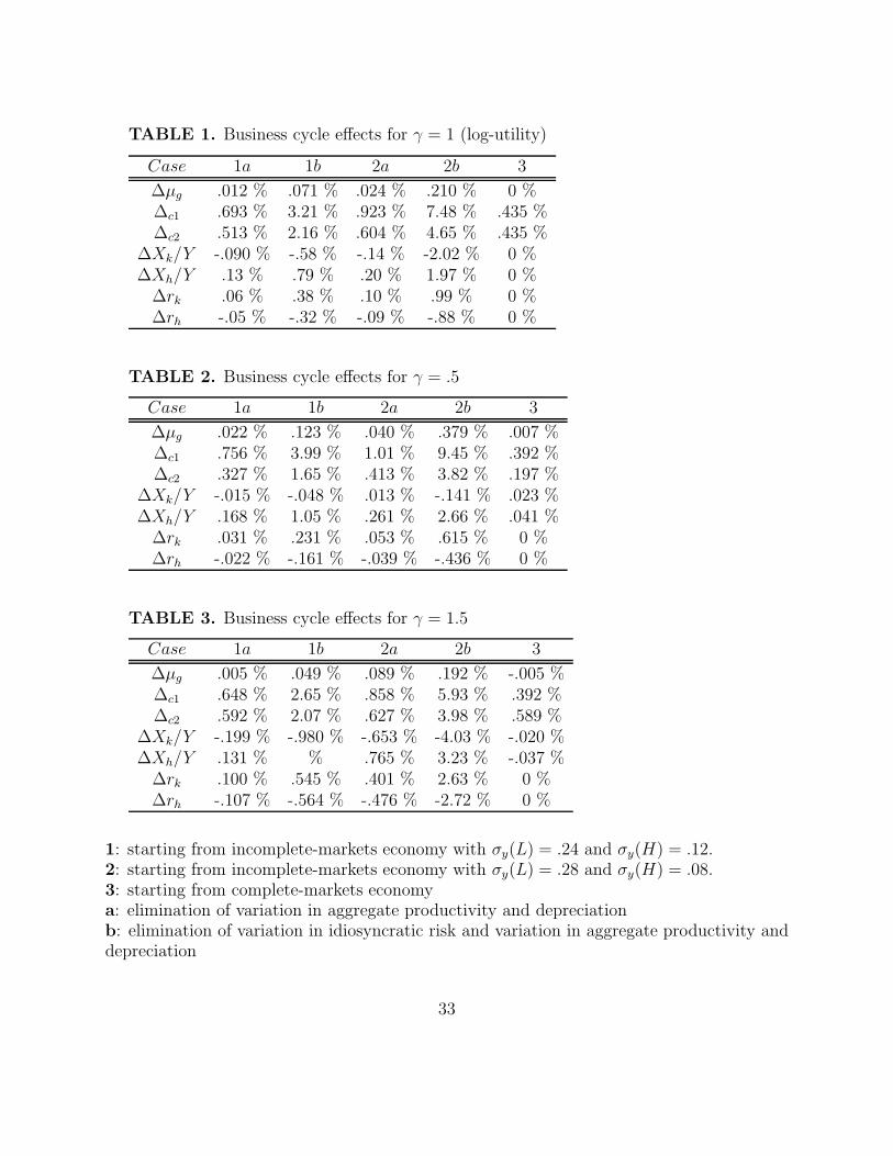
TABLE 1. Business cycle effects for γ = 1 (log-utility)

Case 1a 1b 2a 2b 3

∆µg .012 % .071 % .024 % .210 % 0 %∆c1 .693 % 3.21 % .923 % 7.48 % .435 %∆c2 .513 % 2.16 % .604 % 4.65 % .435 %

∆Xk/Y -.090 % -.58 % -.14 % -2.02 % 0 %∆Xh/Y .13 % .79 % .20 % 1.97 % 0 %

∆rk .06 % .38 % .10 % .99 % 0 %∆rh -.05 % -.32 % -.09 % -.88 % 0 %

TABLE 2. Business cycle effects for γ = .5

Case 1a 1b 2a 2b 3

∆µg .022 % .123 % .040 % .379 % .007 %∆c1 .756 % 3.99 % 1.01 % 9.45 % .392 %∆c2 .327 % 1.65 % .413 % 3.82 % .197 %

∆Xk/Y -.015 % -.048 % .013 % -.141 % .023 %∆Xh/Y .168 % 1.05 % .261 % 2.66 % .041 %

∆rk .031 % .231 % .053 % .615 % 0 %∆rh -.022 % -.161 % -.039 % -.436 % 0 %

TABLE 3. Business cycle effects for γ = 1.5

Case 1a 1b 2a 2b 3

∆µg .005 % .049 % .089 % .192 % -.005 %∆c1 .648 % 2.65 % .858 % 5.93 % .392 %∆c2 .592 % 2.07 % .627 % 3.98 % .589 %

∆Xk/Y -.199 % -.980 % -.653 % -4.03 % -.020 %∆Xh/Y .131 % % .765 % 3.23 % -.037 %

∆rk .100 % .545 % .401 % 2.63 % 0 %∆rh -.107 % -.564 % -.476 % -2.72 % 0 %

1: starting from incomplete-markets economy with σy(L) = .24 and σy(H) = .12.2: starting from incomplete-markets economy with σy(L) = .28 and σy(H) = .08.3: starting from complete-markets economya: elimination of variation in aggregate productivity and depreciationb: elimination of variation in idiosyncratic risk and variation in aggregate productivity anddepreciation

33

∆µg: change in aggregate consumption growth∆c1: change in welfare (in terms of equivalent change in initial consumption)∆c2: change in welfare for constant ∆µg (in terms of equivalent change in initial consump-tion)∆Xk/Y : change in the rate of saving in physical capital∆Xh/Y : change in the rate of saving in human capital∆rk: change in interest rate∆rh: change in wage rate

34