idiosyncratic coskewness and equity return anomalies · idiosyncratic coskewness and equity return...
TRANSCRIPT
Working Paper/Document de travail 2010-11
Idiosyncratic Coskewness and Equity Return Anomalies
by Fousseni Chabi-Yo and Jun Yang
2
Bank of Canada Working Paper 2010-11
May 2010
Idiosyncratic Coskewness and Equity Return Anomalies
by
Fousseni Chabi-Yo1 and Jun Yang2
1Fisher College of Business Ohio State University
Columbus, Ohio, U.S.A. 43210-1144 [email protected]
2Financial Markets Department
Bank of Canada Ottawa, Ontario, Canada K1A 0G9
Bank of Canada working papers are theoretical or empirical works-in-progress on subjects in economics and finance. The views expressed in this paper are those of the authors.
No responsibility for them should be attributed to the Bank of Canada.
ISSN 1701-9397 © 2010 Bank of Canada

ii
Acknowledgements
We are grateful to Bill Bobey, Oliver Boguth, Jean-Sébastien Fontaine, Scott Hendry, Kewei Hou, Michael Lemmon, Jesus Sierra-Jiménez, René Stulz, Ingrid Werner, and seminar participants at the Bank of Canada, the Ohio State University, and the Northern Finance Association 2009 conference. We thank Kenneth French for making a large amount of historical data publicly available in his online data library. We welcome comments, including references to related papers we have inadvertently overlooked. Fousseni Chabi-Yo would like to thank the Dice Center for Financial Economics for financial support.
iii
Abstract
In this paper, we show that in a model where investors have heterogeneous preferences, the expected return of risky assets depends on the idiosyncratic coskewness beta, which measures the co-movement of the individual stock variance and the market return. We find that there is a negative (positive) relation between idiosyncratic coskewness and equity returns when idiosyncratic coskewness betas are positive (negative). Standard risk factors, such as the market, size, book-to-market, and momentum cannot explain the findings. We construct two idiosyncratic coskewness factors to capture the market-wide effect of idiosyncratic coskewness. The two idiosyncratic coskewness factors can also explain the negative and significant relation between the maximum daily return over the past one month (MAX) and expected stock returns documented in Bali, Cakici, and Whitelaw (2009). In addition, when we control for these two idiosyncratic coskewness factors, the return difference for distress-sorted portfolios found in Campbell, Hilscher, and Szilagyi (2008) becomes insignificant. Furthermore, the two idiosyncratic coskewness factors help us understand the idiosyncratic volatility puzzle found in Ang, Hodrick, Xing, and Zhang (2006). They reduce the return difference between portfolios with the smallest and largest idiosyncratic volatility by more than 60%, although the difference is still statistically significant.
JEL classification: G11, G12, G14, G33 Bank classification: Economic models; Financial markets
Résumé
Les auteurs montrent, en modélisant des investisseurs aux préférences hétérogènes, que le rendement espéré d’actifs risqués dépend du coefficient bêta de coasymétrie idiosyncrasique, qui mesure l’évolution conjointe du rendement boursier et de la variance de chaque action. Ils observent une relation négative (positive) entre la coasymétrie idiosyncrasique et les rendements des actions lorsque le coefficient bêta de coasymétrie est positif (négatif). Les facteurs de risque usuels, comme le marché, le volume, le ratio valeur comptable-valeur de marché ou le momentum, ne permettent pas d’expliquer ce résultat. Les auteurs élaborent deux facteurs pour représenter l’incidence de la coasymétrie idiosyncrasique sur l’ensemble du marché. Ces facteurs permettent aussi d’expliquer la relation négative significative qui lie le rendement quotidien maximal enregistré pendant le mois écoulé et les rendements boursiers espérés et dont font état Bali, Cakici et Whitelaw (2009). Une fois ces facteurs idiosyncrasiques pris en compte, l’écart de rendement entre les portefeuilles de Campbell, Hilscher et Szilagyi (2008), constitués après un tri des sociétés émettrices en fonction de leur probabilité de défaut, cesse d’être significatif. Qui plus est, ces deux facteurs aident à percer l’énigme posée par la volatilité idiosyncrasique chez Ang, Hodrick, Xing et Zhang (2006). Leur inclusion réduit en effet de plus de 60 % l’écart de rendement entre les portefeuilles présentant les

iv
niveaux de volatilité idiosyncrasique minimal et maximal; ce dernier demeure toutefois statistiquement significatif.
Classification JEL : G11, G12, G14, G33 Classification de la Banque : Modèles économiques; Marchés financiers
1 Introduction
The single factor capital asset pricing model (CAPM) of Sharpe (1964) and Lintner (1965)
has been empirically tested and rejected by numerous studies, which show that the cross-
sectional variation in expected equity returns cannot be explained by the market beta alone.
One possible extension is to assume that investors care about not only the mean and variance
of their portfolios, but the skewness of their portfolio as well. Harvey and Siddique (2000)
propose an asset pricing model where skewness is priced. In their model, the expected equity
return depends on the market beta and the coskewness beta, which measures the covariance
between an individual equity return and the square of the market return. Mitton and Vorkink
(2008) introduce a model where investors’ preference for the mean and variance is the same
but the preference for skewness is heterogeneous. In their model, the idiosyncratic skewness
is priced. They also show that their model can explain why many investors do not hold
well-diversified portfolios.
We relax certain restrictions in the Mitton and Vorkink (2008) model in this paper. We
show that in a model with heterogeneous preference for skewness, the expected return on
risky assets depends on the market beta, the coskewness beta (as in Harvey and Siddique
(2000)), the idiosyncratic skewness (as in Mitton and Vorkink (2008)), and the idiosyncratic
coskewness beta, which measures the covariance between idiosyncratic variance and the
market return.
We show empirically that when estimated idiosyncratic coskewness betas are positive,
there is a negative relationship between excess returns and idiosyncratic coskewness betas.
When estimated idiosyncratic coskewness betas are negative, the relationship becomes pos-
itive. In addition, when we control for risk using the market factor, the Fama-French three
factors, and the Carhart four factors, the relationship between excess returns and idiosyn-
cratic coskewness betas becomes stronger. In other words, the standard risk factors cannot
explain why portfolios with low idiosyncratic coskewness betas earn high excess returns
when idiosyncratic coskewness betas are positive, and why portfolios with high idiosyncratic
1
coskewness betas earn high excess returns when idiosyncratic coskewness betas are negative.
We form two long-short portfolios, which are long the portfolio with the lowest idiosyncratic
coskewness beta and short the portfolio with the highest idiosyncratic coskewness beta for
both groups with positive and negative idiosyncratic coskewness betas, to capture the sys-
tematic variation in excess portfolio returns sorted by idiosyncratic coskewness betas. We
call them idiosyncratic coskewness factors, ICSK1 for the groups with positive idiosyncratic
coskewness betas, and ICSK2 for the groups with negative idiosyncratic coskewness betas.
The average monthly excess returns for ICSK1 and ICSK2 over the sample period January
1971 to December 2006 are 0.81% (t = 1.87) and -0.63% (t = 2.00) respectively.
In addition, we find that the idiosyncratic coskewness factors can help explain three
anomalous findings in equity market. First, we show that the two idiosyncratic coskewness
factors explain the anomalous finding that stocks with the maximum daily return over the
past month (MAX) earn low expected returns. Bali, Cakici, and Whitelaw (2009) document
a negative and significant relation between the maximum daily return over the past month
and expected stock returns. We show that the average raw and risk-adjusted return differ-
ences between stocks in the lowest and highest MAX deciles is about 0.93% (t = 2.51) per
month. When we regress value-weighted (MAX) portfolios returns on the two idiosyncratic
coskewness factors ICSK1 and ICSK2, the two idiosyncratic coskewness factors reduce the
monthly excess return of a long-short portfolio holding the portfolio with the lowest MAX
measure and shorting the portfolio with the highest MAX measure from 0.93% to 0.26%
(t = 1.34). The results are robust to controls for size, book-to-market and momentum.
Second, there is an anonymous negative relation between equity returns and default risk.
Recent empirical studies (Dichev (1998), Griffin and Lemmon (2002), Campbell, Hilscher,
and Szilagyi (2008)) document a negative relationship between default risk and realized stock
returns. In addition, Campbell, Hilscher, and Szilagyi (2008) find that correcting for risk
using the standard risk factors worsens the anomaly. We show that the two idiosyncratic
coskewness factors can explain the anomalous finding that high stressed firms earn low equity
2
returns. We use the Merton (1974) model to measure default risk for individual firms, and
find the anomalous negative relation between default risk and equity returns. When we
regress distress-sorted portfolio returns on the two idiosyncratic coskewness factors ICSK1
and ICSK2, we find that factor loadings on ICSK1 are generally declining with distress
measures, and factor loadings on ICSK2 are generally increasing with distress measures.
The two idiosyncratic coskewness factors reduce the monthly excess return of a long-short
portfolio holding the portfolio with the lowest distress measure and shorting the portfolio
with the highest distress measure from 1.42% (t = 2.19) to 0.64% (t = 1.01). Including
other standard risk factors, such as the market, size, value, and momentum factors, will not
significantly alter the factors loadings on the two idiosyncratic factors and the alpha of the
long-short portfolio.
Third, we show that the two idiosyncratic coskewness factors can help us understand
the negative relation between idiosyncratic volatility and equity returns found in Ang, Ho-
drick, Xing, and Zhang (2006). They find that stocks with high idiosyncratic volatility earn
abysmally low average returns. This puzzling finding cannot be explained by the standard
risk factors, such as the market, size, book-to-market, momentum, and liquidity. We show
that the two idiosyncratic coskewness factors can explain the monthly return difference be-
tween portfolios with the lowest and second highest idiosyncratic volatility. In addition, the
two idiosyncratic coskewness factors reduce the monthly return difference between portfolios
with the lowest and highest idiosyncratic volatility by more than 60%. However, the return
difference is still statistically significant.
This paper is organized as follows. Section 2 presents both theoretical and empirical
relations between idiosyncratic coskewness betas and equity returns. Section 3 explains
the findings in Bali, Cakici, and Whitelaw (2009) using idiosyncratic coskewness factors.
Section 4 explains the anomalous negative relation between default risk and equity returns
(Campbell, Hilscher, and Szilagyi (2008))using the idiosyncratic coskewness factors. Section
5 addresses the negative relation between equity returns and idiosyncratic volatility found
3
in Ang, Hodrick, Xing, and Zhang (2006). Section 6 concludes.
2 Idiosyncratic Coskewness and Equity Returns
2.1 Theory
Empirical papers have documented that investors usually hold under-diversified portfolios
with a small number of securities. One possible explanation is that investors care about
idiosyncratic skewness in their portfolios. Barberis and Huang (2008) show that idiosyncratic
skewness is priced in equilibrium under the assumption that investors have preferences based
on the cumulative prospect theory1. Mitton and Vorkink (2008) demonstrate the same result
under the assumption of heterogeneous preference for skewness. However, they allow only
idiosyncratic skewness in their model. We extend their model and allow covariance between
the idiosyncratic variance of individual asset returns and the market return, which is named
as idiosyncratic coskewness. We then derive and test the relationship between equity returns
and idiosyncratic coskewness.
We assume that the universe of stocks consists of n risky assets and a risk-free asset.
The return vector of the n securities is denoted as R = [R1, ..., Rn]. The covariance of asset
returns is denoted Σ.
In our economy, we assume that there are two investors, a “traditional” investor and a
“Lotto investor”. Traditional investor utility can be approximated as a standard quadratic
utility function over wealth
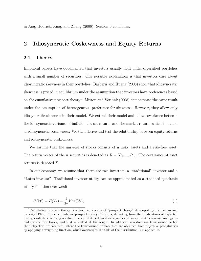
U(W) = E(W)− 1
2τV ar(W), (1)
1Cumulative prospect theory is a modified version of “prospect theory” developed by Kahneman andTversky (1979). Under cumulative prospect theory, investors, departing from the predications of expectedutility, evaluate risk using a value function that is defined over gains and losses, that is concave over gainsand convex over losses, and that is kinked at the origin. In addition, investors use transformed ratherthan objective probabilities, where the transformed probabilities are obtained from objective probabilitiesby applying a weighting function, which overweighs the tails of the distribution it is applied to.
4
where W is the investor terminal wealth, τ > 0 is the coefficient of risk aversion. Levy and
Markowitz (1979) and Hlawitschka (1994) show that the quadratic utility is a reasonable
approximation of standard expected utility functions. And it seems reasonable to assume
that, in the population, the traditional investor behaves as a mean-variance investor. The
“Lotto investor” has the same preferences as the traditional investor over mean and variance,
but also has preference for skewness
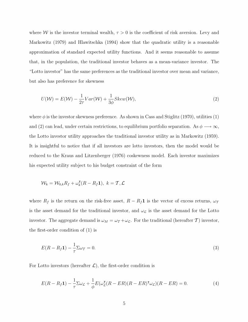
U(W) = E(W)− 1
2τV ar(W) +
1
3φSkew(W), (2)
where φ is the investor skewness preference. As shown in Cass and Stiglitz (1970), utilities (1)
and (2) can lead, under certain restrictions, to equilibrium portfolio separation. As φ −→∞,
the Lotto investor utility approaches the traditional investor utility as in Markowitz (1959).
It is insightful to notice that if all investors are lotto investors, then the model would be
reduced to the Kraus and Litzenberger (1976) coskewness model. Each investor maximizes
his expected utility subject to his budget constraint of the form
Wk = W0,kRf + ωᵀk(R−Rf1), k = T ,L
where Rf is the return on the risk-free asset, R − Rf1 is the vector of excess returns, ωT
is the asset demand for the traditional investor, and ωL is the asset demand for the Lotto
investor. The aggregate demand is ωM = ωT +ωL. For the traditional (hereafter T ) investor,
the first-order condition of (1) is
E(R−Rf1)− 1
τΣωT = 0. (3)
For Lotto investors (hereafter L), the first-order condition is
E(R−Rf1)− 1
τΣωL +
1
φE(ωᵀ
L(R− ER)(R− ER)ᵀωL)(R− ER) = 0. (4)
5
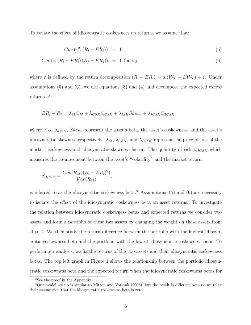
To isolate the effect of idiosyncratic coskewness on returns, we assume that:
Cov(ε2, (Ri − ERi)
)= 0. (5)
Cov (ε, (Ri − ERi) (Rj − ERj)) = 0 for i, j. (6)
where ε is defined by the return decomposition (Ri − ERi) = ai(WT − EWT ) + ε. Under
assumptions (5) and (6), we use equations (3) and (4) and decompose the expected excess
return as2:
ERi −Rf = λMβiM + λCSKβiCSK + λISKSkewi + λICSKβiICSK
where βiM , βiCSK , Skewi represent the asset’s beta, the asset’s coskewness, and the asset’s
idiosyncratic skewness respectively. λM , λCSK , and λICSK represent the price of risk of the
market, coskewness and idiosyncratic skewness factor. The quantity of risk βiICSK which
measures the co-movement between the asset’s “volatility” and the market return.
βiICSK =Cov(RM , (Ri − ERi)
2)
V ar(RM),
is referred to as the idiosyncratic coskewness beta.3 Assumptions (5) and (6) are necessary
to isolate the effect of the idiosyncratic coskewness beta on asset returns. To investigate
the relation between idiosyncratic coskewness betas and expected returns we consider two
assets and form a portfolio of these two assets by changing the weight on these assets from
-1 to 1. We then study the return difference between the portfolio with the highest idiosyn-
cratic coskewness beta and the portfolio with the lowest idiosyncratic coskewness beta. To
perform our analysis, we fix the returns of the two assets and their idiosyncratic coskewness
betas. The top left graph in Figure 1 shows the relationship between the portfolio idiosyn-
cratic coskewness beta and the expected return when the idiosyncratic coskewness betas for
2See the proof in the Appendix.3Our model set up is similar to Mitton and Vorkink (2008), but the result is different because we relax
their assumption that the idiosyncratic coskewness beta is zero.
6
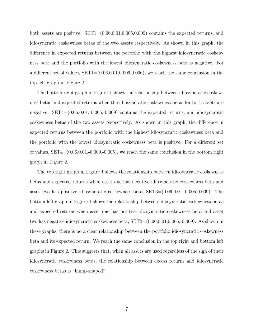
both assets are positive. SET1=(0.06,0.01,0.005,0.009) contains the expected returns, and
idiosyncratic coskewness betas of the two assets respectively. As shown in this graph, the
difference in expected returns between the portfolio with the highest idiosyncratic coskew-
ness beta and the portfolio with the lowest idiosyncratic coskewness beta is negative. For
a different set of values, SET1=(0.06,0.01,0.009,0.006), we reach the same conclusion in the
top left graph in Figure 2.
The bottom right graph in Figure 1 shows the relationship between idiosyncratic coskew-
ness betas and expected returns when the idiosyncratic coskewness betas for both assets are
negative. SET4=(0.06,0.01,-0.005,-0.009) contains the expected returns, and idiosyncratic
coskewness betas of the two assets respectively. As shown in this graph, the difference in
expected returns between the portfolio with the highest idiosyncratic coskewness beta and
the portfolio with the lowest idiosyncratic coskewness beta is positive. For a different set
of values, SET4=(0.06,0.01,-0.009,-0.005), we reach the same conclusion in the bottom right
graph in Figure 2.
The top right graph in Figure 1 shows the relationship between idiosyncratic coskewness
betas and expected returns when asset one has negative idiosyncratic coskewness beta and
asset two has positive idiosyncratic coskewness beta, SET3=(0.06,0.01,-0.005,0.009). The
bottom left graph in Figure 1 shows the relationship between idiosyncratic coskewness betas
and expected returns when asset one has positive idiosyncratic coskewness beta and asset
two has negative idiosyncratic coskewness beta, SET3=(0.06,0.01,0.005,-0.009). As shown in
these graphs, there is no a clear relationship between the portfolio idiosyncratic coskewness
beta and its expected return. We reach the same conclusion in the top right and bottom left
graphs in Figure 2. This suggests that, when all assets are used regardless of the sign of their
idiosyncratic coskewness betas, the relationship between excess returns and idiosyncratic
coskewness betas is “hump-shaped”.
7
2.2 Equity Returns and Measures of Higher Moments Risk
In this section, we use the entire CRSP equity data set to investigate the relationship be-
tween equity returns and coskewness betas, idiosyncratic coskewness betas, and idiosyncratic
skewness respectively. At the beginning of each month, we use the past 12-month daily data
on individual stock returns to compute coskewness betas, idiosyncratic coskewness betas,
and idiosyncratic skewness respectively as defined in the previous section, and form portfo-
lios sorted by coskewness betas, idiosyncratic coskewness betas, and idiosyncratic skewness
respectively. To reduce the liquidity effect on equity returns, we eliminate firms with no
transaction days larger than 120. We also eliminate stocks with prices less than $1 at the
end of a month. Following the same method used to compute returns for distress-sorted
portfolios, we compute value-weighted returns for portfolios sorted by coskewness betas,
idiosyncratic coskewness betas, and idiosyncratic skewness respectively.
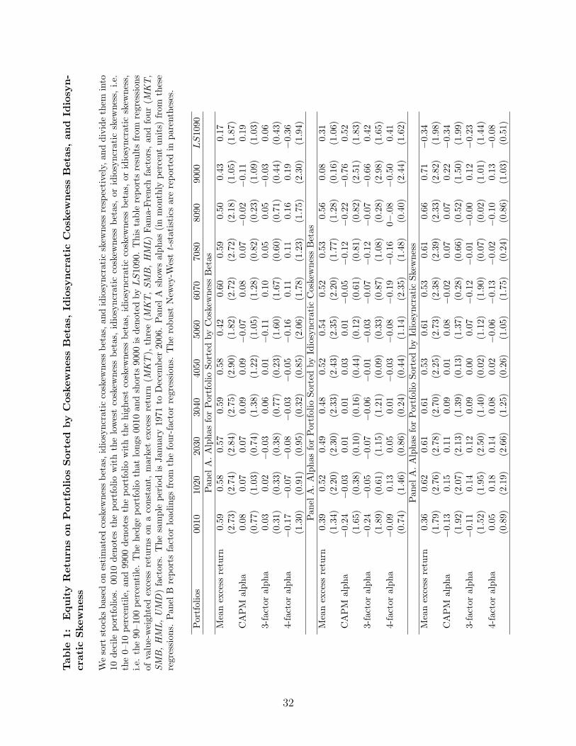
Table 1 reports the results for the decile portfolios sorted by coskewness betas, idiosyn-
cratic coskewness betas, and idiosyncratic skewness respectively. For the ten portfolios sorted
by coskewness betas, there is a slight negative relation between excess equity returns and
coskewness betas, which is consistent with Harvey and Siddique (2000). However, the re-
lationship almost disappears when we control for the Fama-French factors. In addition,
the relationship becomes positive when we control the Carhart four factors. For the ten
portfolios sorted by idiosyncratic coskewness betas, the relationship between excess equity
returns and idiosyncratic coskewness betas is hump-shaped, i.e. portfolios with both lowest
and highest idiosyncratic coskewness betas have lower excess returns than the others. This
hump-shaped relationship does not disappear even when we control the market factor, the
Fama-French factors, or the Carhart factors. This result is consistent with our theoretical
prediction. For the ten portfolios sorted by idiosyncratic skewness, there is a slight positive
relation between excess equity returns and idiosyncratic skewness. However, this relationship
basically disappears when we control the standard risk factors, such as the market factor,
the Fama-French factors, or the Carhart factors. Table 1 confirms our theoretical finding
8
that the idiosyncratic coskewness measure is different from the standard coskewness and
idiosyncratic skewness measure. It is important to point out that empirically testing the
relation between idiosyncratic skewness and returns is not a straightforward exercise. The
primary obstacle is that ex ante skewness is difficult to measure. As opposed to variances
and covariances, idiosyncratic skewness is not stable over time. This explains the marginal
effect of idiosyncratic skewness on expected returns4.
To further investigate the cross-sectional relation between idiosyncratic coskewness betas
and idiosyncratic skewness, we run a simple OLS regression of idiosyncratic coskewness
betas on idiosyncratic skewness each month using the estimated idiosyncratic coskewness
betas and idiosyncratic skewness for all available firms. The time series of estimated slope
coefficients and R2s are plotted in Figure 3. It shows that there is a positive relation between
cross-sectional idiosyncratic coskewness and idiosyncratic skewness during the sample period.
However, the positive relation is very weak given that the average R2s from the regressions
is 1.8%. The results demonstrate that idiosyncratic coskewness betas and idiosyncratic
skewness measure different aspects of equity returns.
2.3 Equity Returns Sorted by Positive and Negative Idiosyncratic
Coskewness
We showed in the last section that there is a hump-shaped relation between equity returns
and idiosyncratic coskewness betas. To further investigate that relationship, we divide firms
into two groups according to the sign of their idiosyncratic coskewness betas. For each group,
we then rank the stocks based on their past idiosyncratic coskewness betas and form ten
value-weighted decile portfolios. Following the same method used to compute returns for
distress-sorted portfolios, we compute value-weighted returns for idiosyncratic coskewness
4To avoid this obstacle, Boyer, Mitton, and Vorkink (2009) regress idiosyncratic skeweness on a set ofpredictor variables and use the expected component of their linear regression as a measure of expectedidiosyncratic skewness. Because the goal of this paper is to investigate whether idiosyncratic coskewnessbetas explain the default risk puzzle, we do not investigate the empirical relationship between expectedidiosyncratic skewness and expected idiosyncratic coskewness. We leave this issue for future research.
9
beta-sorted portfolios in each group.
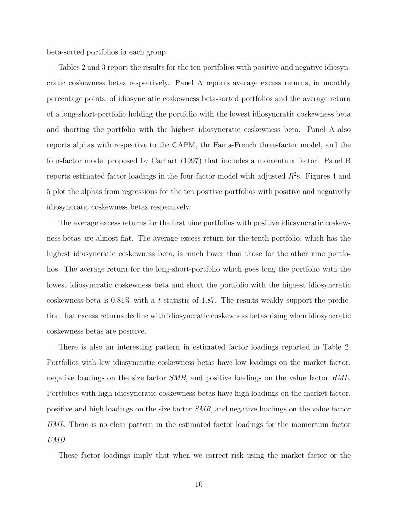
Tables 2 and 3 report the results for the ten portfolios with positive and negative idiosyn-
cratic coskewness betas respectively. Panel A reports average excess returns, in monthly
percentage points, of idiosyncratic coskewness beta-sorted portfolios and the average return
of a long-short-portfolio holding the portfolio with the lowest idiosyncratic coskewness beta
and shorting the portfolio with the highest idiosyncratic coskewness beta. Panel A also
reports alphas with respective to the CAPM, the Fama-French three-factor model, and the
four-factor model proposed by Carhart (1997) that includes a momentum factor. Panel B
reports estimated factor loadings in the four-factor model with adjusted R2s. Figures 4 and
5 plot the alphas from regressions for the ten positive portfolios with positive and negatively
idiosyncratic coskewness betas respectively.
The average excess returns for the first nine portfolios with positive idiosyncratic coskew-
ness betas are almost flat. The average excess return for the tenth portfolio, which has the
highest idiosyncratic coskewness beta, is much lower than those for the other nine portfo-
lios. The average return for the long-short-portfolio which goes long the portfolio with the
lowest idiosyncratic coskewness beta and short the portfolio with the highest idiosyncratic
coskewness beta is 0.81% with a t-statistic of 1.87. The results weakly support the predic-
tion that excess returns decline with idiosyncratic coskewness betas rising when idiosyncratic
coskewness betas are positive.
There is also an interesting pattern in estimated factor loadings reported in Table 2.
Portfolios with low idiosyncratic coskewness betas have low loadings on the market factor,
negative loadings on the size factor SMB, and positive loadings on the value factor HML.
Portfolios with high idiosyncratic coskewness betas have high loadings on the market factor,
positive and high loadings on the size factor SMB, and negative loadings on the value factor
HML. There is no clear pattern in the estimated factor loadings for the momentum factor
UMD.
These factor loadings imply that when we correct risk using the market factor or the
10
Fama-French three factors, we will not be able to explain why the portfolio with the high-
est idiosyncratic coskewness beta has such low excess returns compared to the other nine
portfolios. On the contrary, it will worsen the anomaly. In fact, alphas in the regressions
with respect to the CAPM, the Fama-French three-factor model, and Carhart four-factor
model are almost monotonically declining with idiosyncratic coskewness betas increasing. A
long-short portfolio that holds the portfolio with the lowest idiosyncratic coskewness beta
and shorts the portfolio with the highest idiosyncratic coskewness beta has a CAPM alpha
of 1.21% with a t-statistic of 3.14; it has a Fama-French three-factor alpha of 1.12% with
a t-statistic of 4.29; and it has a Carhart four-factor alpha of 0.98% with a t-statistic of
4.02. When we correct risk using the standard factors, we find stronger evidence to support
the prediction that there is a negative relationship between excess returns and idiosyncratic
coskewness betas when idiosyncratic coskewness betas are negative.
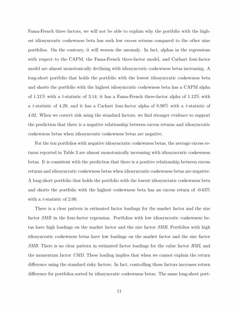
For the ten portfolios with negative idiosyncratic coskewness betas, the average excess re-
turns reported in Table 3 are almost monotonically increasing with idiosyncratic coskewness
betas. It is consistent with the prediction that there is a positive relationship between excess
returns and idiosyncratic coskewness betas when idiosyncratic coskewness betas are negative.
A long-short portfolio that holds the portfolio with the lowest idiosyncratic coskewness beta
and shorts the portfolio with the highest coskewness beta has an excess return of -0.63%
with a t-statistic of 2.00.
There is a clear pattern in estimated factor loadings for the market factor and the size
factor SMB in the four-factor regression. Portfolios with low idiosyncratic coskewness be-
tas have high loadings on the market factor and the size factor SMB. Portfolios with high
idiosyncratic coskewness betas have low loadings on the market factor and the size factor
SMB. There is no clear pattern in estimated factor loadings for the value factor HML and
the momentum factor UMD. These loading implies that when we cannot explain the return
difference using the standard risky factors. In fact, controlling those factors increases return
difference for portfolios sorted by idiosyncratic coskewness betas. The same long-short port-
11
folio has a CAPM alpha of -0.88% with a t-statistic of 2.74; it has a Fama-French three-factor
alpha of -0.85% with a t-statistic of 3.76; and it has a Carhart four-factor alpha of -0.61%
with a t-statistic of 2.48.
In summary, the empirical results support that the relationship between equity returns
and idiosyncratic coskewness betas is positive when idiosyncratic coskewness betas are neg-
ative, and negative when idiosyncratic coskewness betas are positive. In addition, we find
that the return difference between portfolios sorted by idiosyncratic coskewness betas, with
either positive or negative values, cannot be explained by the standard risk factors, such as
the market factor, the size factor, the value factor, and the momentum factor. In the next
section, we will examine the relationship between default risk and idiosyncratic coskewness.
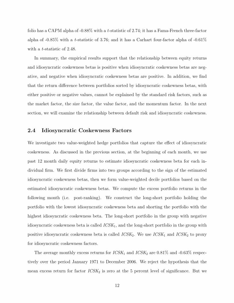
2.4 Idiosyncratic Coskewness Factors
We investigate two value-weighted hedge portfolios that capture the effect of idiosyncratic
coskewness. As discussed in the previous section, at the beginning of each month, we use
past 12 month daily equity returns to estimate idiosyncratic coskewness beta for each in-
dividual firm. We first divide firms into two groups according to the sign of the estimated
idiosyncratic coskewness betas, then we form value-weighted decile portfolios based on the
estimated idiosyncratic coskewness betas. We compute the excess portfolio returns in the
following month (i.e. post-ranking). We construct the long-short portfolio holding the
portfolio with the lowest idiosyncratic coskewness beta and shorting the portfolio with the
highest idiosyncratic coskewness beta. The long-short portfolio in the group with negative
idiosyncratic coskewness beta is called ICSK1, and the long-short portfolio in the group with
positive idiosyncratic coskewness beta is called ICSK2. We use ICSK1 and ICSK2 to proxy
for idiosyncratic coskewness factors.
The average monthly excess returns for ICSK1 and ICSK2 are 0.81% and -0.63% respec-
tively over the period January 1971 to December 2006. We reject the hypothesis that the
mean excess return for factor ICSK2 is zero at the 5 percent level of significance. But we
12

cannot reject the same hypothesis for factor ICSK1. A high factor loading on ICSK1 should
be associated with high expected excess returns. In contrast, for factor ICSK2, a high factor
loading should be associated with low expected excess returns.
2.5 Can Idiosyncratic Coskewness Factors Explain the Fama and
French Portfolios?
The failures of the CAPM model often appear in specific groups of securities that are formed
on size, book-to-market ratio and momentum. To understand how idiosyncratic coskewness
factors enter asset pricing, we analyze the pricing errors from other asset pricing models
such as the Fama-French three-factor model, and the four-factor model proposed by Carhart
(1997).
We carry out time-series regressions of excess returns,
ri,t = αi +K∑
j=1
β̂jfj,t + ei,t, for i = 1, ..., N, t = 1, ..., T, (7)
and jointly test whether the intercepts, αi, are different from zero using the F-test of Gibbons,
Ross, and Shanken (1989) where F ∼ (N, T − N − K). We test the Fama-French three
factor model and Carhart four-factor model for industrial portfolios, decile portfolios sorted
by size, book-to-market ratio, and momentum, and decile portfolios sorted by idiosyncratic
coskewness beta. The results are presented in Table 4. When we test 10 portfolios sorted by
the book-to-market ratio, the inclusion of the two idiosyncratic coskewness factors reduces
the F-statistics from 4.96 to 1.95 in the Fama-French model and from 3.39 to 1.31 in the
Carhart model. Similar results are obtained for momentum-sorted portfolios and portfolios
sorted by idiosyncratic coskewness beta. In all cases, the inclusion of the two idiosyncratic
coskewness factors in either the Fama-French model or the Carhart model dramatically
reduces the F-statistics. The results suggest that the two idiosyncratic coskewness factors
can explain a significant part of the variation in returns even when factors based on size,
13
book-to-market ratio, and momentum are added to the asset pricing model.
3 MAX Returns and Idiosyncratic Coskewness
A recent empirical paper by Bali, Cakici, and Whitelaw (2009) investigates the significance of
extreme positive returns in the cross-sectional pricing of stocks. Their portfolio-level analysis
and firm-level cross-sectional regressions indicate a negative and significant relation between
the maximum daily return over the past month (MAX) and expected stock returns. Average
raw and risk-adjusted return differences between stocks in the lowest and highest MAX
deciles exceed 1% per month. Their results are robust to controls for size, book-to-market,
momentum, short-term reversals, liquidity, and skewness. The idiosyncratic coskewness
beta proposed in this paper directly measures the relationship between the expected return
of a stock and its contribution to the skewness of the portfolio. We investigate whether
our idiosyncratic coskewness factors can explain the puzzling finding in Bali, Cakici, and
Whitelaw (2009). We first replicate their findings using the CRSP data set, then we examine
the linkage between idiosyncratic coskewness and their anomalous findings by regressing
portfolio sorted by the maximum daily return over the past month on the standard and the
two idiosyncratic coskewness factors. The results are reported in table 5.
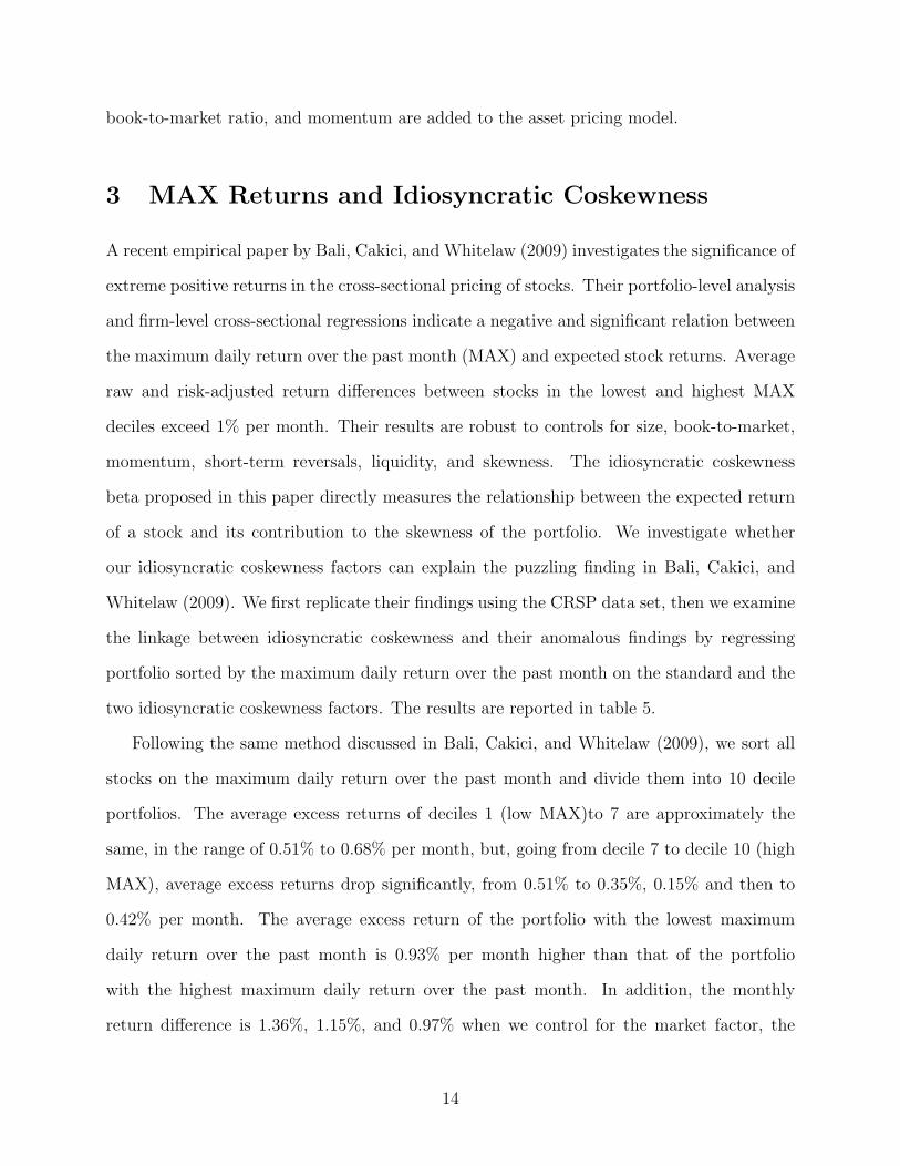
Following the same method discussed in Bali, Cakici, and Whitelaw (2009), we sort all
stocks on the maximum daily return over the past month and divide them into 10 decile
portfolios. The average excess returns of deciles 1 (low MAX)to 7 are approximately the
same, in the range of 0.51% to 0.68% per month, but, going from decile 7 to decile 10 (high
MAX), average excess returns drop significantly, from 0.51% to 0.35%, 0.15% and then to
0.42% per month. The average excess return of the portfolio with the lowest maximum
daily return over the past month is 0.93% per month higher than that of the portfolio
with the highest maximum daily return over the past month. In addition, the monthly
return difference is 1.36%, 1.15%, and 0.97% when we control for the market factor, the
14

Fama-French factors, and the Carhart factors, respectively. The return differences are all
statistically significant. The results are consistent with the findings in Bali, Cakici, and
Whitelaw (2009). They interpret the results as “Given a preference for upside potential,
investors may be willing to pay more for, and accept lower expected returns on, assets with
these extremely high positive returns.”
When we add the two idiosyncratic coskewness factors into the regression of returns of the
10 decile portfolios on the market factor, the monthly return difference between the portfolio
with the lowest and the highest maximum daily return over the past month is reduced from
1.36% to 0.43% with a t-statistics 1.92. When we add the two idiosyncratic factors into the
regressions using Fama-French 3 factors and Carhart 4 factors, the monthly return difference
between the portfolio with the lowest and the highest maximum daily return over the past
month is reduced from 1.15% (t = 4.66) to 0.40% (t = 1.78), and from 0.97% (t = 3.61)
to 0.34% (t = 1.51), respectively. In addition, we have sorted all stocks on the average of
the maximum two and three daily returns over the past month respectively. We obtain very
similar results when we add the two idiosyncratic coskewness factors to the regressions.
Bali, Cakici, and Whitelaw (2009) rely on the cumulative prospect theory as modeled
in Barberis and Huang (2008) to explain their findings. We provide an alternative rational
explanation based on the assumption of heterogeneous preference. The “Lotto investor” who
cares not only about the mean and variance of his portfolio but also about the skewness of
his portfolio would bid up those lottery-like stocks to improve his portfolio allocation.
4 Default Risk and Idiosyncratic Coskewness
4.1 Equity Returns on Distressed Stocks
Recent empirical studies by Dichev (1998), Griffin and Lemmon (2002), and Campbell,
Hilscher, and Szilagyi (2008) find a surprising negative relation between expected equity
returns and default risk. If the stocks of financially distressed firms tend to move together,
15
and their risk cannot be diversified away, finance theory dictates a positive relation between
expected equity returns and default risk. If default risk is idiosyncratic, there is no signif-
icant relation between expected returns and default risk. These empirical findings seem to
suggest that the equity market has not properly priced default risk. We examine if the two
idiosyncratic coskewness factors can explain the negative relation between equity returns
and default risk.
We use the Merton (1974) model to estimate the default probability for each firm (see
appendix B), and examine the relationship between the likelihood of default and equity
returns. We use the same method to estimate default likelihood as Vassalou and Xing (2004).
Unlike Vassalou and Xing (2004), we use only industrial firms, which are more suitable for
Merton’s model. We also minimize liquidity effects on equity returns by eliminating illiquid
stocks. At the end of each month, we sort firms according to their default measures and
construct 10 portfolios as discussed in the previous section. Because highly distressed firms
are more likely to be delisted and disappear from the CRSP database, it is important to
carefully compute equity returns for delisted firms. CRSP reports a delisting return for
the final month of a firm’s life when it is available. In this case, we use delisting returns
to compute portfolio returns. When delisting returns are not available, we exclude those
firms from portfolios. This assumes that those stocks are sold at the end of the month
before delisting, which implies an upward bias to the returns for distressed-stock portfolios
(Shumway (1997)).
Table 7 reports the summary statistics of equity returns on the ten distress-sorted port-
folios. The average returns are declining in general with default measures increasing. The
average return is 0.92% for the portfolio with the lowest default risk, and it is -0.51% for the
portfolio with the highest default risk. The volatilities of returns are increasing with default
measures. The standard deviation of returns is 4.48% for the portfolio with the lowest de-
fault risk, and it is 14.95% for the portfolio with the highest default risk. In addition, returns
on portfolios with low default measures exhibit negative skewness, and returns on portfo-
16
lios with high default measures exhibit positive skewness. There is no clear pattern in the
kurtosis of returns. Table 7 also reports the unconditional coskewness betas, idiosyncratic
coskewness betas, and idiosyncratic skewness of the ten distress-sorted portfolios. There is
no clear pattern in the coskewness betas. However, both idiosyncratic coskewness betas and
idiosyncratic skewness are in general increasing with default measures. The average size of
firms in the ten portfolios is monotonically declining with default measures increasing. It
suggests that controlling for the size risk factor will not explain the puzzling negative relation
between equity returns and default risk.
A possible explanation for the negative relation between equity returns and default mea-
sures is that the default measure is just a proxy for other systematic risk factors. We test
this hypothesis with regression results in Table 8. Panel A reports the excess returns of
ten distress-sorted portfolios and a long-short-portfolio that goes long the portfolio with the
lowest default risk, and short the portfolio with the highest default risk. Panel A also reports
the alphas in regressions of the portfolio excess returns on the CAPM factor, Fama-French
three factors, and four factors proposed by Carhart (1997) that includes a momentum factor
in addition to Fama-French three factors. The returns are reported in monthly percentage
points, with Robust Newey-West t-statistics below in the parentheses. Panel B, C, and D
report estimated factor loadings for excess returns on the CAPM factor, Fama-French three
factors, and four factors in the Carhart (1997) model. Figure 7 plots the alphas from these
regressions.
The average excess returns of the 10 stress-sorted portfolios reported in Table 8 are in
general declining in the default risk measure. The average excess return for the lowest-risk
5% of stocks is positive at 0.43% per month, and the average excess return for the highest-
risk 1% of stocks is negative at -0.99% per month. A long-short portfolio that goes long
the safest 5% of stocks, and short the most distressed 1% of stocks has an average return of
1.42% per month with a standard deviation of 14%. It implies a Sharp ratio of 0.10.
There is also a significant pattern on the factor loadings reported in Table 8. The low risk
17
portfolios in general have smaller market betas, negative loadings on the size factor SMB,
and negative loadings on the value factor HML. On the contrary, the high risk portfolios
in general have bigger market betas, positive loadings on the size factor SMB, and positive
loadings on the value factor HML. The results reflect the fact that most distressed stocks
are small stocks with high book-to-market ratios. It implies that correcting risk using the
market factor or Fama-French factors will not solve the anomaly but worsen it. In fact,
the long-short portfolio that is long the safest 5% of stocks, and short the most distressed
1% of stocks has a CAPM alpha of 1.94% per month with a t-statistic of 3.16. It has a
Fama-French three-factor alpha of 2.76% per month with a t-statistic of 4.90. In addition,
the Fama-French three-factor alphas for all portfolios beyond 40th percentile of the default
risk distribution are negative and statistically significant.
Avramov, Chordia, Jostova, and Philipov (2007) find a robust link between credit rating
and momentum. They find that momentum profit exists only in low-grade firms. Distressed
firms have negative momentum, which may explain their low average returns. When we
correct for risk by using the Carhart (1997) four-factor model including a momentum factor,
the low risk portfolios in general have low and positive loadings on the momentum factor.
The high risk portfolios have high and negative loadings on the momentum factor. After
controlling for the momentum factor, we find that the alpha for the long-short portfolio is
cut almost in half, from 2.76% per month to 1.38% per month, which is still statistically
significant.
4.2 Explaining Equity Return for Distressed Firms
We have demonstrated that in a model with heterogeneous investors who care about the
skewness of their portfolios, the expected return of risky assets depends on their market
betas, coskewness betas, idiosyncratic coskewness betas and idiosyncratic skewness. To
capture the effect of coskewness on cross-sectional equity returns, we construct a value-
weighted hedge portfolio, i.e. the coskewness factor, holding the portfolio with the lowest
18
coskewness beta and shorting the portfolio with the highest coskewness beta. In a similar
fashion, we also construct a hedge portfolio, i.e. the idiosyncratic skewness factor, to capture
the effect of idiosyncratic skewness.
We have shown that the standard risk factors, such as the market factor, the Fama-French
factors, and the Carhart four risk factors, cannot explain why high distressed firms earn low
equity returns. In our model, expected equity returns depend on not only their CAPM betas,
but also their coskewness betas, idiosyncratic coskewness betas and idiosyncratic skewness.
We investigate if coskewness betas, idiosyncratic coskewness betas or idiosyncratic skewness
can help explain the anomaly. We first run simple regressions of returns of distress-sorted
portfolios on the market factor, the coskewness factor, the two idiosyncratic coskewness
factors, and the idiosyncratic skewness factor. The results presented in Table 9 show that
the equity return anomaly for distressed firms still exists when we control for any of the
market factor, the coskewness factor, and the idiosyncratic skewness factor. The monthly
return difference between portfolios with the lowest and highest default probabilities is 1.94%
(t = 3.16), 1.41% (t = 2.18), and 1.66% (t = 2.55), respectively, when we control for the
market factor, the coskewness factor, and the idiosyncratic skewness factor. The return
differences are statistically significant at the 5% level. However, the monthly return difference
between portfolios with the lowest and highest default probabilities is 0.73% (t = 1.12) and
0.89% (t = 1.45), respectively, when we control for the positive and negative idiosyncratic
coskewness factors. The return differences are not statistically significant at the 5% level.
The simple regression results show that either positive or negative idiosyncratic coskew-
ness factors can at least partially explain why equity returns are low for high distressed
firms. High distressed firms will earn low equity returns if they have negative loadings on
the positive idiosyncratic coskewness factor and positive loadings on the negative idiosyn-
cratic coskewness factor. We will further test this hypothesis by regressing distress-sorted
portfolio returns on two idiosyncratic coskewness factors, ICSK1 and ICSK2. We will also
test the robustness of our results by including other risk factors, such as the Fama-French
19
factors and the momentum factor, in the regressions. The regression results are reported in
Table 10.
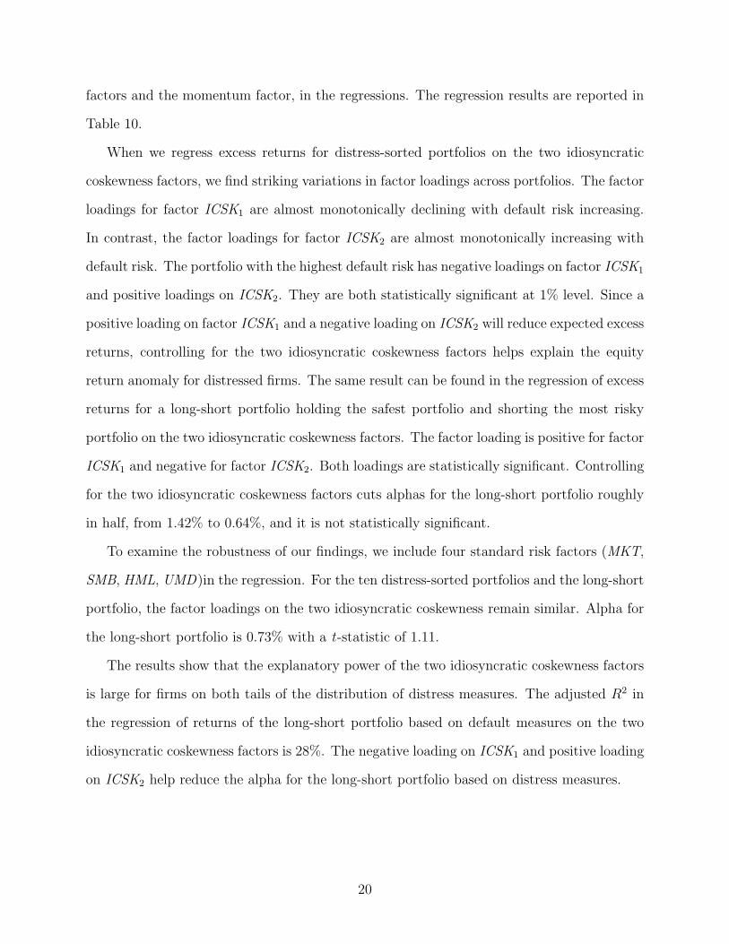
When we regress excess returns for distress-sorted portfolios on the two idiosyncratic
coskewness factors, we find striking variations in factor loadings across portfolios. The factor
loadings for factor ICSK1 are almost monotonically declining with default risk increasing.
In contrast, the factor loadings for factor ICSK2 are almost monotonically increasing with
default risk. The portfolio with the highest default risk has negative loadings on factor ICSK1
and positive loadings on ICSK2. They are both statistically significant at 1% level. Since a
positive loading on factor ICSK1 and a negative loading on ICSK2 will reduce expected excess
returns, controlling for the two idiosyncratic coskewness factors helps explain the equity
return anomaly for distressed firms. The same result can be found in the regression of excess
returns for a long-short portfolio holding the safest portfolio and shorting the most risky
portfolio on the two idiosyncratic coskewness factors. The factor loading is positive for factor
ICSK1 and negative for factor ICSK2. Both loadings are statistically significant. Controlling
for the two idiosyncratic coskewness factors cuts alphas for the long-short portfolio roughly
in half, from 1.42% to 0.64%, and it is not statistically significant.
To examine the robustness of our findings, we include four standard risk factors (MKT,
SMB, HML, UMD)in the regression. For the ten distress-sorted portfolios and the long-short
portfolio, the factor loadings on the two idiosyncratic coskewness remain similar. Alpha for
the long-short portfolio is 0.73% with a t-statistic of 1.11.
The results show that the explanatory power of the two idiosyncratic coskewness factors
is large for firms on both tails of the distribution of distress measures. The adjusted R2 in
the regression of returns of the long-short portfolio based on default measures on the two
idiosyncratic coskewness factors is 28%. The negative loading on ICSK1 and positive loading
on ICSK2 help reduce the alpha for the long-short portfolio based on distress measures.
20
5 Idiosyncratic Volatility Puzzle and Idiosyncratic Coskew-
ness
An empirical study by Ang, Hodrick, Xing, and Zhang (2006) finds a negative relation
between the expected return and a stocks’s idiosyncratic volatility (IVOL) relative to the
Fama and French (1993) three-factor model. This negative relationship cannot be explained
by a number of standard risk factors, such as the aggregate volatility, size, book-to-market,
momentum, and liquidity. Next we investigate if the two idiosyncratic coskewness factors
can explain this phenomenon.
We compute idiosyncratic volatility using residuals from a regression of past 1-year daily
equity returns on the Fama-French three factors. We then sort stocks into 10 decile portfolios
according to the computed idiosyncratic volatility. We computed the equity returns for each
portfolio for the following month. The results are presented in Table 11.
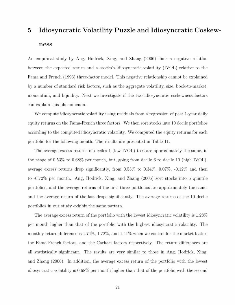
The average excess returns of deciles 1 (low IVOL) to 6 are approximately the same, in
the range of 0.53% to 0.68% per month, but, going from decile 6 to decile 10 (high IVOL),
average excess returns drop significantly, from 0.55% to 0.34%, 0.07%, -0.12% and then
to -0.72% per month. Ang, Hodrick, Xing, and Zhang (2006) sort stocks into 5 quintile
portfolios, and the average returns of the first three portfolios are approximately the same,
and the average return of the last drops significantly. The average returns of the 10 decile
portfolios in our study exhibit the same pattern.
The average excess return of the portfolio with the lowest idiosyncratic volatility is 1.28%
per month higher than that of the portfolio with the highest idiosyncratic volatility. The
monthly return difference is 1.74%, 1.72%, and 1.41% when we control for the market factor,
the Fama-French factors, and the Carhart factors respectively. The return differences are
all statistically significant. The results are very similar to those in Ang, Hodrick, Xing,
and Zhang (2006). In addition, the average excess return of the portfolio with the lowest
idiosyncratic volatility is 0.68% per month higher than that of the portfolio with the second
21
highest idiosyncratic volatility. The monthly return difference is 1.15%, 0.95%, and 0.77%
when we control for the market factor, the Fama-French factors, and the Carhart factors,
respectively. The return differences are all statistically significant when we control for the
standard risk factors.
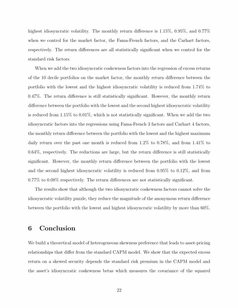
When we add the two idiosyncratic coskewness factors into the regression of excess returns
of the 10 decile portfolios on the market factor, the monthly return difference between the
portfolio with the lowest and the highest idiosyncratic volatility is reduced from 1.74% to
0.47%. The return difference is still statistically significant. However, the monthly return
difference between the portfolio with the lowest and the second highest idiosyncratic volatility
is reduced from 1.15% to 0.01%, which is not statistically significant. When we add the two
idiosyncratic factors into the regressions using Fama-French 3 factors and Carhart 4 factors,
the monthly return difference between the portfolio with the lowest and the highest maximum
daily return over the past one month is reduced from 1.2% to 0.78%, and from 1.41% to
0.64%, respectively. The reductions are large, but the return difference is still statistically
significant. However, the monthly return difference between the portfolio with the lowest
and the second highest idiosyncratic volatility is reduced from 0.95% to 0.12%, and from
0.77% to 0.08% respectively. The return differences are not statistically significant.
The results show that although the two idiosyncratic coskewness factors cannot solve the
idiosyncratic volatility puzzle, they reduce the magnitude of the anonymous return difference
between the portfolio with the lowest and highest idiosyncratic volatility by more than 60%.
6 Conclusion
We build a theoretical model of heterogeneous skewness preference that leads to asset-pricing
relationships that differ from the standard CAPM model. We show that the expected excess
return on a skewed security depends the standard risk premium in the CAPM model and
the asset’s idiosyncratic coskewness betas which measures the covariance of the squared
22
idiosyncratic shock and the market return.
We empirically show that in addition to the well known idiosyncratic skewness, the
idiosyncratic coskewness measure is also an important determinant for asset returns. Our
measure of idiosyncratic coskewness cannot be explain by the idiosyncratic skewness, this
suggests that both idiosyncratic skewness and idiosyncratic coskewness measure different
higher moment risks. The idiosyncratic coskewness can explain the anomalous finding that
stocks with the maximum daily return over the past month (MAX) earn low expected returns
(see Bali, Cakici, and Whitelaw (2009)).
We also provide a rational explanation of the seemingly anomalous negative relation
between default risk and equity returns. Although a number of theories point toward a
lower return for stocks with default risk, empirical testing of the relation between default
risk and measures of idiosyncratic skewness has been slow in coming. We attempt to fill
this void by estimating a model of idiosyncratic coskewness and then using idiosyncratic
coskewness to explain the negative relation between default risk and equity returns. We
find that once we control for idiosyncratic coskewness, the negative relation between equity
returns and default risk disappears.
Furthermore, the idiosyncratic coskewness seems to be related to the idiosyncratic volatil-
ity puzzle found in Ang, Hodrick, Xing, and Zhang (2006). Although the idiosyncratic
coskewness factors cannot totally explain the negative relation between equity return and
idiosyncratic volatility, they significantly reduced the magnitude of the return difference
between portfolios with the smallest and largest idiosyncratic volatility.
23
Appendix A: Equity Returns and Idiosyncratic Coskew-
ness
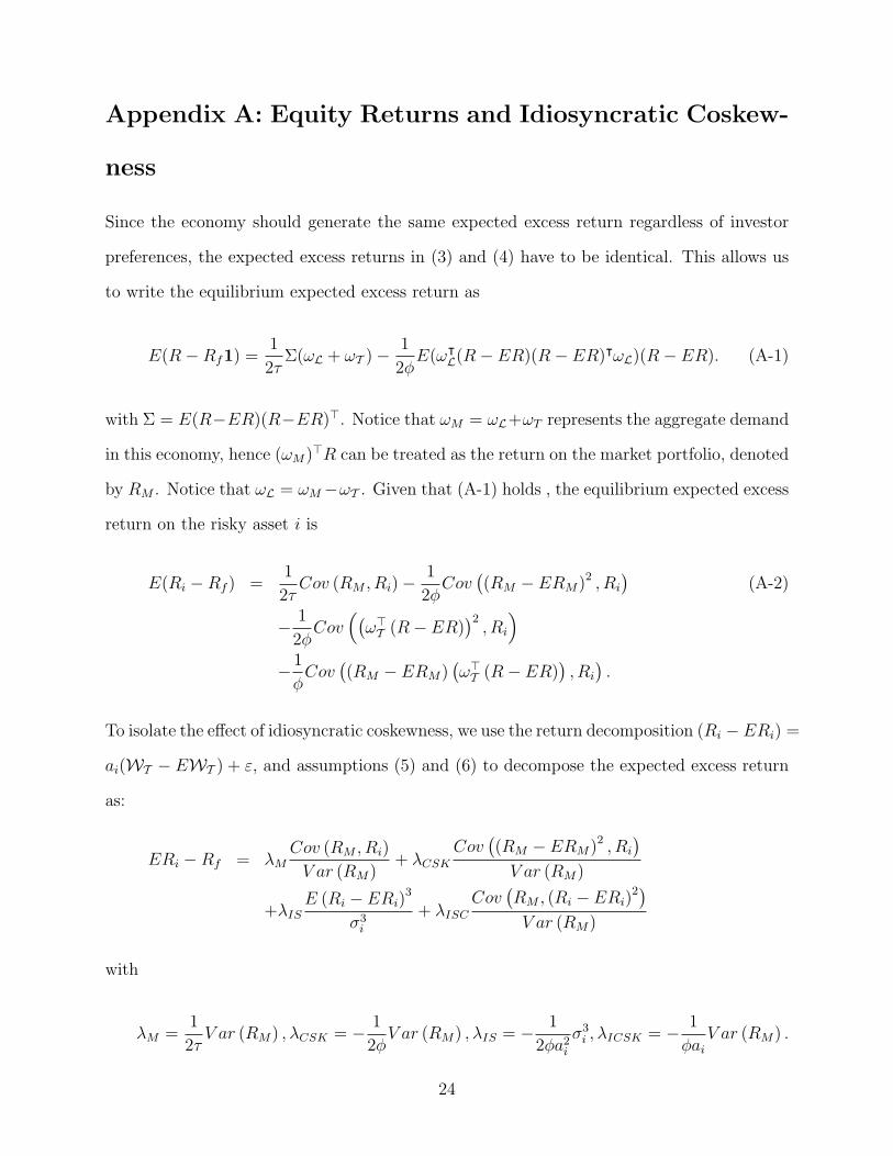
Since the economy should generate the same expected excess return regardless of investor
preferences, the expected excess returns in (3) and (4) have to be identical. This allows us
to write the equilibrium expected excess return as
E(R−Rf1) =1
2τΣ(ωL + ωT )− 1
2φE(ωᵀ
L(R− ER)(R− ER)ᵀωL)(R− ER). (A-1)
with Σ = E(R−ER)(R−ER)>. Notice that ωM = ωL+ωT represents the aggregate demand
in this economy, hence (ωM)>R can be treated as the return on the market portfolio, denoted
by RM . Notice that ωL = ωM−ωT . Given that (A-1) holds , the equilibrium expected excess
return on the risky asset i is
E(Ri −Rf ) =1
2τCov (RM , Ri)− 1
2φCov
((RM − ERM)2 , Ri
)(A-2)
− 1
2φCov
((ω>T (R− ER)
)2, Ri
)
−1
φCov
((RM − ERM)
(ω>T (R− ER)
), Ri
).
To isolate the effect of idiosyncratic coskewness, we use the return decomposition (Ri − ERi) =
ai(WT − EWT ) + ε, and assumptions (5) and (6) to decompose the expected excess return
as:
ERi −Rf = λMCov (RM , Ri)
V ar (RM)+ λCSK
Cov((RM − ERM)2 , Ri
)
V ar (RM)
+λISE (Ri − ERi)
3
σ3i
+ λISC
Cov(RM , (Ri − ERi)
2)
V ar (RM)
with
λM =1
2τV ar (RM) , λCSK = − 1
2φV ar (RM) , λIS = − 1
2φa2i
σ3i , λICSK = − 1
φai
V ar (RM) .
24
Appendix B.1: Measuring Default Probability with the
Merton’s Model
In the default risk literature, there are two approaches to measure default risk, the reduced-
form and structural approaches. A reduced-form model provides the maximum likelihood
estimates of a firm’s default probability based on the empirical frequency of default and
its correlation with various firm characteristics. A structural model provides an estimated
default probability which is theoretically motivated by the classical option-pricing models
(Merton (1974)). Traditional reduced-form models, such as Altman (1968) Z-score model
and Ohlson (1980) O-score model, compute measures of bankruptcy by using accounting
information in conditional logia models. Accounting models use information from firms’
financial statement. The accounting information is about firms’ past performance, rather
than their future prospects. In contrast, structural models use the market value of equity
to derive measures of default risk. Market prices reflect investors’ expectations about firms’
future performance. Therefore, they are better suited for measuring the probability that a
firm may default in the future. In this paper, we use Merton’s (1974) model to estimate
the default probability of a firm. In Merton’s model, the equity of a firm is viewed as a call
option on the value of firm’s assets. The firm will default when the value of the firm falls
below a strike price, which is measured as the book value of firm’s liabilities. The firm value
is not observable and is assumed to follow a geometric Browning motion of the form:
dVA = µAVAdt + σAVAdW, (A-3)
where VA is the value of firm’s assets, with an instantaneous drift µA, and an instantaneous
volatility σA. W is the standard Wiener process.
Let Xt denote the book value of firm’s liabilities at time t, which has a maturity at time
25

T . The value of equity is given by the Black and Schools (1973) formula for call options:
VE = VAN(d1) + Xe−rT N(d2), (A-4)
where
d1 =ln(VA/X) + (r + 1
2σ2
A)T
σA
√T
, d2 = d1 − σA
√T , (A-5)
r is the risk-free interest rate, and N is the cumulative density function of the standard
normal distribution.
Using daily equity data from the past 12 months, we adopt a maximum likelihood method
developed by Duan (1998) to obtain an estimate of the volatility of firm value σA. Duan
(1998) computes the likelihood function of equity returns by utilizing the conditional density
of the unobservable firm value process. We repeat the estimation procedure at the end
of every month, resulting in monthly estimates of the volatility σA. We always keep the
estimation window to 12 months.
With an estimated σA, we can calculate daily values of VA for the last 12 months, and
then estimate the drift µA. At the end of every month t, the probability of default implied
by Merton’s model is given by:
Pdef,t = N(ln(VA,t/Xt) + (µA − 1
2σ2
A)T
σA
√T
). (A-6)
The Pdef,t calculated from equation (A-6) does not correspond to the true default prob-
ability of a firm in large samples since we do not use data on actual defaults. However, we
use our measures to study the relationship between default risk and equity returns. The
difference between our measure of default probability and true default probability may not
be important as long as our measure correctly ranks firms according to their true default
probability.
26
Appendix B.2: Data
One important parameter in Merton’s model is the strike price, i.e. the book value of debt.
Most firms have both long-term and short-term debts. Following KM, we calculate the book
value of debt by using short-term debt plus half long-term debt. We use the COMPUSTAT
annual files to obtain the firm’s “Debt in One Year” and “Long-Term Debt” series for all
firms. Since debt data was not available for many firms before 1970, the sample period
in our study is January 1971 to December 2006. In addition, financial firms have very
different capital structure than industrial firms. We exclude all financial firms (SIC codes:
6000–6999). We also exclude all utility firms (SIC codes: 4900–4999) because many utility
firms were highly regulated during our sample period. We use only industrial firms (SIC
codes: 1–3999 and 5000–5999) in this studies since they are more suitable for Merton’s
model. We obtain all industrial firms with data available simultaneously on both CRSP and
COMPUSTAT databases.
We obtain the book value of debt from the COMPUSTAT annual files. To avoid the
problem of delayed reporting, we lag the book value of debt by 3 months. This is to ensure
that our default probability measure is based on all information available to investors at the
time of calculation.
To compute the default likelihood measure, we obtain daily equity values for firms from
CRSP daily files, and the risk-free interest rate from the Fama-Bliss discount bond file. We
use monthly observations of the 1-year Treasury bill rate and equity data for the past 12
months to calculate monthly default measures for all firms.
When a firm is in sever financial distress, its equity is not liquid with low prices. To
minimize liquidity effects on equity returns, we eliminate stocks with prices less than $1 at
the portfolio construction date, and stocks with less than 120 transactions in the past 12
months. In the end, we have 10,078 firms with more than 3.5 million monthly observations
in the sample.
Figure 6 plots the average default probability for industrial firms during the sample
27
period. The shaded areas represent the NBER recession periods. The graph shows that the
average default probability varies greatly and it usually peaks during recessions.
Appendix B.3: Performance of Merton’s Model
To test the performance of Merton’s model in predicting bankruptcy and other distress in our
sample, we construct two measures based on exchange delisting as proxies for bankruptcy.
One is a narrower measure of distress, called bankruptcy delisting (delisting codes: 400,
572, 574). The other is a broader measure of distress, called performance delisting (delisting
codes: 400, 550 to 585). The second measure includes delisting due to not only bankruptcy
and liquidation but also insufficient number of market makers, insufficient capital, surplus,
and/or equity, price too low, delinquent in filing, etc. All the delisting data are obtained
from CRSP.
To evaluate the predictive ability of our default measure to capture default risk, we sort
firms according to their estimated default probability based on past 12-month equity data.
At the end of each month from January 1971 through December 2006, default probability is
re-estimated using only historical data to avoid look-ahead bias. To pay greater attention to
the tail of the default risk distribution, we follow Campbell et. al. and construct 10 portfolios
containing stocks in percentiles 0–5, 5–10, 10–20, 20–40, 40–60, 60–80, 80–90, 90–95, 95–
99, and 99–100 (P1 and P10 denote the portfolios with the lowest and the highest default
probability respectively). In the following month, we then collect the number of bankruptcy
and performance delistings for each portfolio. The summary results are reported in Table 6.
The evidence shows that the default risk measure based on Merton’s model is a good ex ante
measure of probability of bankruptcy and other distress. The number of bankruptcy and
performance delistings generally increases with default risk measures from Merton’s model.
During the sample period, 46 out of 60 delistings due to bankruptcy and liquidation, and 213
out of 443 delistings due to performance come from the two portfolios with highest default
measures. These two portfolios contains the highest-risk 5% of stocks.
28
References
Altman, Edward I., 1968, Financial ratios, discriminant analysis and the prediction of cor-
porate bankruptcy, Journal of Finance 23, 589–609.
Ang, Andrew, Robert J. Hodrick, Yuhang Xing, and Xiaoyan Zhang, 2006, The cross-section
of volatility and expected returns, Journal of Finance 61, 259–299.
Avramov, Doron, Tarun Chordia, Gergana Jostova, and Alexander Philipov, 2007, Momen-
tum and credit rating, Journal of Finance 62, 2503–2520.
Bali, Turan G., Nusret Cakici, and Robert Whitelaw, 2009, Maxing out: Stocks as lotteries
and the cross-section of expected returns, Working Paper.
Barberis, Nicholas, and Ming Huang, 2008, Stocks as lotteries: the implications of probability
weighting for security prices, American Economic Review 98, 2066–2100.
Boyer, Brian, Todd Mitton, and Keith Vorkink, 2009, Expected idiosyncratic skewness,
Review of Financial Studies forthcoming.
Campbell, John Y., Jens Hilscher, and Jan Szilagyi, 2008, In search of distress risk, Journal
of Finance 63, 2899–2939.
Carhart, Mark, 1997, On persistence in mutual fund performance, Journal of Finance 52,
57–82.
Cass, David, and Joseph Stiglitz, 1970, The structure of investor preferences and asset
returns, and separability in portfolio allocation: A contribution to the pure theory of
mutual funds, Journal of Economic Theory 2, 122–160.
Dichev, Ilia, 1998, Is the risk of bankruptcy a systematic risk?, Journal of Finance 53,
1141–1148.
29

Duan, Jin-Chuan, 1998, Maximum likelihood estimation using price data of the derivative
contract, Mathematical Finance 4, 155–167.
Fama, Eugene F., and Kenneth R. French, 1993, Common risk factors in the returns on
stocks and bonds, Journal of Financial Economics 33, 3–56.
Gibbons, Michael R., Stephen A. Ross, and Jay Shanken, 1989, A test of the efficiency of a
given portfolio, Econometrica 57, 1121–1152.
Griffin, John M., and Michael L. Lemmon, 2002, Book-to-market equity, distress risk,and
stock returns, Journal of Finance 57, 2317–2336.
Harvey, Campbell R., and Akhtar Siddique, 2000, Conditional skewness in asset pricing
tests, Journal of Finance 55, 1263–1295.
Hlawitschka, Walter, 1994, The empirical nature of taylor-series approximations to expected
utility, American Economic Review 84, 713–719.
Kahneman, Daniel, and SAmos Tversky, 1979, Prospect theory: An analysis of decision
under risk, Econometrica 47, 263–291.
Kraus, Alan, and Robert H. Litzenberger, 1976, Skewness preference and the valuation of
risk assets, Journal of Finance 31, 1085–1100.
Levy, Haim, and Harry M. Markowitz, 1979, Approximating expected utility by a function
of mean and variance, American Economic Review 69, 308–317.
Lintner, John, 1965, The valuation of risk assets and the selection of risky investments in
stock portfolios and capital budgets, Review of Economics and Statistics 47, 13–37.
Markowitz, Harry M., 1959, Portfolio Selection: Efficient Diversification of Investment (New
York: John Wiley & Sons).
30
Merton, Robert C., 1974, On the pricing of corporate debt: the risk structure of interest
rates, Journal of Finance 29, 449–470.
Mitton, Todd, and Keith Vorkink, 2008, Equilibrium underdiversification and the preference
for skewness, Review of Financial Studies 20, 1255–1288.
Ohlson, James A., 1980, Financial ratios and the probabilistic prediction of bankruptcy,
Journal of Accounting Research 18, 109–131.
Sharpe, William, 1964, Capital asset prices: A theory of market equilibrium under conditions
of risk, Journal of Finance 19, 425–442.
Shumway, Tyler, 1997, The delisting bias in crsp data, Journal of Finance 52, 327–340.
Vassalou, Maria, and Yuhang Xing, 2004, Default risk in equity returns, Journal of Finance
59, 831–868.
31
Tab
le1:
Equity
Ret
urn
son
Por
tfol
ios
Sor
ted
by
Cos
kew
nes
sB
etas
,Id
iosy
ncr
atic
Cos
kew
nes
sB
etas
,an
dId
iosy
n-
crat
icSke
wnes
s
We
sort
stoc
ksba
sed
ones
tim
ated
cosk
ewne
ssbe
tas,
idio
sync
rati
cco
skew
ness
beta
s,an
did
iosy
ncra
tic
skew
ness
resp
ecti
vely
,and
divi
deth
emin
to10
deci
lepo
rtfo
lios.
0010
deno
tes
the
port
folio
wit
hth
elo
wes
tco
skew
ness
beta
s,id
iosy
ncra
tic
cosk
ewne
ssbe
tas,
orid
iosy
ncra
tic
skew
ness
,i.e
.th
e0–
10pe
rcen
tile
,an
d99
00de
note
sth
epo
rtfo
liow
ith
the
high
est
cosk
ewne
ssbe
tas,
idio
sync
rati
cco
skew
ness
beta
s,or
idio
sync
rati
csk
ewne
ss,
i.e.
the
90–1
00pe
rcen
tile
.T
hehe
dge
port
folio
that
long
s00
10an
dsh
orts
9000
isde
note
dby
LS
1090
.T
his
tabl
ere
port
sre
sult
sfr
omre
gres
sion
sof
valu
e-w
eigh
ted
exce
ssre
turn
son
aco
nsta
nt,m
arke
tex
cess
retu
rn(M
KT
),th
ree
(MK
T,SM
B,H
ML)
Fam
a-Fr
ench
fact
ors,
and
four
(MK
T,
SMB,H
ML,U
MD
)fa
ctor
s.T
hesa
mpl
epe
riod
isJa
nuar
y19
71to
Dec
embe
r20
06.
Pan
elA
show
sal
phas
(in
mon
thly
perc
ent
unit
s)fr
omth
ese
regr
essi
ons.
Pan
elB
repo
rts
fact
orlo
adin
gsfr
omth
efo
ur-fac
tor
regr
essi
ons.
The
robu
stN
ewey
-Wes
tt-
stat
isti
csar
ere
port
edin
pare
nthe
ses.
Por
tfol
ios
0010
1020
2030
3040
4050
5060
6070
7080
8090
9000
LS
1090
Pan
elA
.A
lpha
sfo
rPor
tfol
ioSo
rted
byC
oske
wne
ssB
etas
Mea
nex
cess
retu
rn0.
590.
580.
570.
590.
580.
420.
600.
590.
500.
430.
17(2
.73)
(2.7
4)(2
.84)
(2.7
5)(2
.90)
(1.8
2)(2
.72)
(2.7
2)(2
.18)
(1.0
5)(1
.87)
CA
PM
alph
a0.
080.
070.
070.
090.
09−0
.07
0.08
0.07
−0.0
2−0
.11
0.19
(0.7
7)(1
.03)
(0.7
4)(1
.38)
(1.2
2)(1
.05)
(1.2
8)(0
.82)
(0.2
3)(1
.09)
(1.0
3)3-
fact
oral
pha
0.03
0.02
−0.0
30.
060.
01−0
.11
0.10
0.05
0.05
−0.0
30.
06(0
.31)
(0.3
3)(0
.38)
(0.7
7)(0
.23)
(1.6
0)(1
.67)
(0.6
0)(0
.71)
(0.4
4)(0
.43)
4-fa
ctor
alph
a−0
.17
−0.0
7−0
.08
−0.0
3−0
.05
−0.1
60.
110.
110.
160.
19−0
.36
(1.3
0)(0
.91)
(0.9
5)(0
.32)
(0.8
5)(2
.06)
(1.7
8)(1
.23)
(1.7
5)(2
.30)
(1.9
4)Pan
elA
.A
lpha
sfo
rPor
tfol
ioSo
rted
byId
iosy
ncra
tic
Cos
kew
ness
Bet
asM
ean
exce
ssre
turn
0.39
0.52
0.49
0.48
0.52
0.54
0.52
0.53
0.56
0.08
0.31
(1.3
4)(2
.20)
(2.3
0)(2
.33)
(2.4
3)(2
.35)
(2.2
0)(1
.77)
(1.2
8)(0
.16)
(1.0
6)C
AP
Mal
pha
−0.2
4−0
.03
0.01
0.01
0.03
0.01
−0.0
5−0
.12
−0.2
2−0
.76
0.52
(1.6
5)(0
.38)
(0.1
0)(0
.16)
(0.4
4)(0
.12)
(0.6
1)(0
.81)
(0.8
2)(2
.51)
(1.8
3)3-
fact
oral
pha
−0.2
4−0
.05
−0.0
7−0
.06
−0.0
1−0
.03
−0.0
7−0
.12
−0.0
7−0
.66
0.42
(1.8
9)(0
.61)
(1.1
5)(1
.21)
(0.0
9)(0
.33)
(0.8
7)(1
.08)
(0.2
8)(2
.98)
(1.6
5)4-
fact
oral
pha
−0.0
90.
130.
050.
01−0
.03
−0.0
8−0
.19
−0.1
60−
.08
−0.5
00.
41(0
.74)
(1.4
6)(0
.86)
(0.2
4)(0
.44)
(1.1
4)(2
.35)
(1.4
8)(0
.40)
(2.4
4)(1
.62)
Pan
elA
.A
lpha
sfo
rPor
tfol
ioSo
rted
byId
iosy
ncra
tic
Skew
ness
Mea
nex
cess
retu
rn0.
360.
620.
610.
610.
530.
610.
530.
610.
660.
71−0
.34
(1.7
9)(2
.76)
(2.7
8)(2
.70)
(2.2
5)(2
.73)
(2.3
8)(2
.39)
(2.3
3)(2
.82)
(1.9
8)C
AP
Mal
pha
−0.1
30.
150.
110.
090.
010.
08−0
.02
0.07
0.07
0.22
−0.3
4(1
.92)
(2.0
7)(2
.13)
(1.3
9)(0
.13)
(1.3
7)(0
.28)
(0.6
6)(0
.52)
(1.5
0)(1
.99)
3-fa
ctor
alph
a−0
.11
0.14
0.12
0.09
0.00
0.07
−0.1
2−0
.01
−0.0
00.
12−0
.23
(1.5
2)(1
.95)
(2.5
0)(1
.40)
(0.0
2)(1
.12)
(1.9
0)(0
.07)
(0.0
2)(1
.01)
(1.4
4)4-
fact
oral
pha
0.05
0.18
0.14
0.08
0.02
−0.0
6−0
.13
−0.0
2−0
.10
0.13
−0.0
8(0
.89)
(2.1
9)(2
.66)
(1.2
5)(0
.26)
(1.0
5)(1
.75)
(0.2
4)(0
.86)
(1.0
3)(0
.51)
32
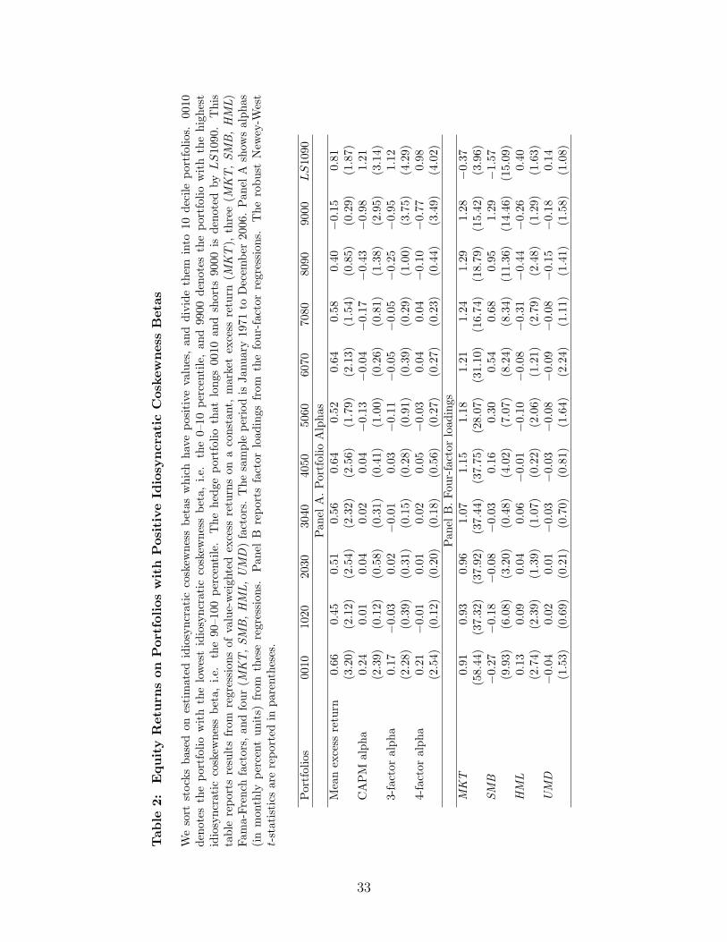
Tab
le2:
Equity
Ret
urn
son
Por
tfol
ios
wit
hPos
itiv
eId
iosy
ncr
atic
Cos
kew
nes
sB
etas
We
sort
stoc
ksba
sed
ones
tim
ated
idio
sync
rati
cco
skew
ness
beta
sw
hich
have
posi
tive
valu
es,
and
divi
deth
emin
to10
deci
lepo
rtfo
lios.
0010
deno
tes
the
port
folio
wit
hth
elo
wes
tid
iosy
ncra
tic
cosk
ewne
ssbe
ta,
i.e.
the
0–10
perc
enti
le,
and
9900
deno
tes
the
port
folio
wit
hth
ehi
ghes
tid
iosy
ncra
tic
cosk
ewne
ssbe
ta,
i.e.
the
90–1
00pe
rcen
tile
.T
hehe
dge
port
folio
that
long
s00
10an
dsh
orts
9000
isde
note
dby
LS
1090
.T
his
tabl
ere
port
sre
sult
sfr
omre
gres
sion
sof
valu
e-w
eigh
ted
exce
ssre
turn
son
aco
nsta
nt,
mar
ket
exce
ssre
turn
(MK
T),
thre
e(M
KT
,SM
B,
HM
L)
Fam
a-Fr
ench
fact
ors,
and
four
(MK
T,SM
B,H
ML,U
MD
)fa
ctor
s.T
hesa
mpl
epe
riod
isJa
nuar
y19
71to
Dec
embe
r20
06.
Pan
elA
show
sal
phas
(in
mon
thly
perc
ent
unit
s)fr
omth
ese
regr
essi
ons.
Pan
elB
repo
rts
fact
orlo
adin
gsfr
omth
efo
ur-fac
tor
regr
essi
ons.
The
robu
stN
ewey
-Wes
tt-
stat
isti
csar
ere
port
edin
pare
nthe
ses.
Por
tfol
ios
0010
1020
2030
3040
4050
5060
6070
7080
8090
9000
LS
1090
Pan
elA
.Por
tfol
ioA
lpha
sM
ean
exce
ssre
turn
0.66
0.45
0.51
0.56
0.64
0.52
0.64
0.58
0.40
−0.1
50.
81(3
.20)
(2.1
2)(2
.54)
(2.3
2)(2
.56)
(1.7
9)(2
.13)
(1.5
4)(0
.85)
(0.2
9)(1
.87)
CA
PM
alph
a0.
240.
010.
040.
020.
04−0
.13
−0.0
4−0
.17
−0.4
3−0
.98
1.21
(2.3
9)(0
.12)
(0.5
8)(0
.31)
(0.4
1)(1
.00)
(0.2
6)(0
.81)
(1.3
8)(2
.95)
(3.1
4)3-
fact
oral
pha
0.17
−0.0
30.
02−0
.01
0.03
−0.1
1−0
.05
−0.0
5−0
.25
−0.9
51.
12(2
.28)
(0.3
9)(0
.31)
(0.1
5)(0
.28)
(0.9
1)(0
.39)
(0.2
9)(1
.00)
(3.7
5)(4
.29)
4-fa
ctor
alph
a0.
21−0
.01
0.01
0.02
0.05
−0.0
30.
040.
04−0
.10
−0.7
70.
98(2
.54)
(0.1
2)(0
.20)
(0.1
8)(0
.56)
(0.2
7)(0
.27)
(0.2
3)(0
.44)
(3.4
9)(4
.02)
Pan
elB
.Fo
ur-fac
tor
load
ings
MK
T0.
910.
930.
961.
071.
151.
181.
211.
241.
291.
28−0
.37
(58.
44)
(37.
32)
(37.
92)
(37.
44)
(37.
75)
(28.
07)
(31.
10)
(16.
74)
(18.
79)
(15.
42)
(3.9
6)SM
B−0
.27
−0.1
8−0
.08
−0.0
30.
160.
300.
540.
680.
951.
29−1
.57
(9.9
3)(6
.08)
(3.2
0)(0
.48)
(4.0
2)(7
.07)
(8.2
4)(8
.34)
(11.
36)
(14.
46)
(15.
09)
HM
L0.
130.
090.
040.
06−0
.01
−0.1
0−0
.08
−0.3
1−0
.44
−0.2
60.
40(2
.74)
(2.3
9)(1
.39)
(1.0
7)(0
.22)
(2.0
6)(1
.21)
(2.7
9)(2
.48)
(1.2
9)(1
.63)
UM
D−0
.04
0.02
0.01
−0.0
3−0
.03
−0.0
8−0
.09
−0.0
8−0
.15
−0.1
80.
14(1
.53)
(0.6
9)(0
.21)
(0.7
0)(0
.81)
(1.6
4)(2
.24)
(1.1
1)(1
.41)
(1.5
8)(1
.08)
33
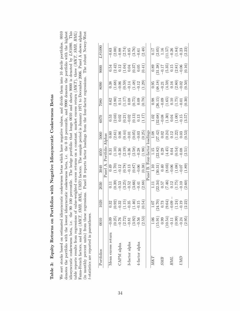
Tab
le3:
Equity
Ret
urn
son
Por
tfol
ios
wit
hN
egat
ive
Idio
syncr
atic
Cos
kew
nes
sB
etas
We
sort
stoc
ksba
sed
ones
tim
ated
idio
sync
rati
cco
skew
ness
beta
sw
hich
have
nega
tive
valu
es,
and
divi
deth
emin
to10
deci
lepo
rtfo
lios.
0010
deno
tes
the
port
folio
wit
hth
elo
wes
tid
iosy
ncra
tic
cosk
ewne
ssbe
ta,
i.e.
the
0–10
perc
enti
le,
and
9900
deno
tes
the
port
folio
wit
hth
ehi
ghes
tid
iosy
ncra
tic
cosk
ewne
ssbe
ta,
i.e.
the
90–1
00pe
rcen
tile
.T
hehe
dge
port
folio
that
long
s00
10an
dsh
orts
9000
isde
note
dby
LS
1090
.T
his
tabl
ere
port
sre
sult
sfr
omre
gres
sion
sof
valu
e-w
eigh
ted
exce
ssre
turn
son
aco
nsta
nt,
mar
ket
exce
ssre
turn
(MK
T),
thre
e(M
KT
,SM
B,
HM
L)
Fam
a-Fr
ench
fact
ors,
and
four
(MK
T,SM
B,H
ML,U
MD
)fa
ctor
s.T
hesa
mpl
epe
riod
isJa
nuar
y19
71to
Dec
embe
r20
06.
Pan
elA
show
sal
phas
(in
mon
thly
perc
ent
unit
s)fr
omth
ese
regr
essi
ons.
Pan
elB
repo
rts
fact
orlo
adin
gsfr
omth
efo
ur-fac
tor
regr
essi
ons.
The
robu
stN
ewey
-Wes
tt-
stat
isti
csar
ere
port
edin
pare
nthe
ses.
Por
tfol
ios
0010
1020
2030
3040
4050
5060
6070
7080
8090
9000
LS
1090
Pan
elA
.Por
tfol
ioA
lpha
sM
ean
exce
ssre
turn
−0.0
90.
320.
110.
490.
310.
600.
530.
620.
380.
54−0
.63
(0.2
5)(0
.92)
(0.3
9)(1
.70)
(1.1
0)(2
.61)
(2.0
3)(2
.80)
(1.6
8)(2
.42)
(2.0
0)C
AP
Mal
pha
−0.7
6−0
.32
−0.5
3−0
.12
−0.3
00.
060.
020.
14−0
.06
0.12
−0.8
8(2
.72)
(1.1
5)(3
.25)
(0.7
8)(2
.19)
(0.4
4)(0
.21)
(1.1
7)(0
.59)
(1.0
4)(2
.74)
3-fa
ctor
alph
a−0
.81
−0.3
5−0
.52
−0.1
3−0
.36
−0.0
1−0
.02
0.08
−0.1
40.
04−0
.85
(3.9
2)(1
.46)
(3.6
6)(0
.87)
(2.5
8)(0
.05)
(0.1
3)(0
.75)
(1.4
8)(0
.37)
(3.7
6)4-
fact
oral
pha
−0.5
6−0
.15
−0.4
1−0
.06
−0.2
8−0
.03
0.13
0.09
−0.1
20.
05−0
.61
(2.5
3)(0
.54)
(2.8
8)(0
.38)
(1.9
8)(0
.25)
(1.1
7)(0
.78)
(1.2
9)(0
.41)
(2.4
8)Pan
elB
.Fo
ur-fac
tor
load
ings
MK
T1.
061.
071.
111.
101.
151.
081.
020.
980.
950.
890.
17(1
5.91
)(2
4.70
)(2
2.34
)(3
0.31
)(2
2.82
)(2
7.42
)(3
2.68
)(2
6.15
)(4
8.18
)(3
1.38
)(2
.05)
SMB
0.99
0.73
0.57
0.40
0.29
0.02
−0.0
8−0
.09
−0.2
1−0
.17
1.16
(10.
54)
(9.6
4)(7
.46)
(8.0
3)(4
.45)
(0.2
4)(1
.30)
(1.6
5)(4
.59)
(5.3
5)(1
1.57
)H
ML
−0.1
1−0
.09−
0.12
−0.0
60.
040.
120.
040.
100.
160.
15−0
.26
(0.9
9)(1
.24)
(1.7
5)(1
.08)
(0.5
4)(1
.22)
(1.0
0)(1
.75)
(2.8
0)(2
.81)
(1.8
4)U
MD
−0.2
4−0
.19
−0.1
0−0
.07
−0.0
80.
03−0
.15
−0.0
1−0
.02
−0.0
6−0
.23
(2.9
5)(2
.22)
(2.6
0)(1
.89)
(2.5
1)(0
.53)
(3.5
7)(0
.30)
(0.5
0)(0
.16)
(2.2
3)
34
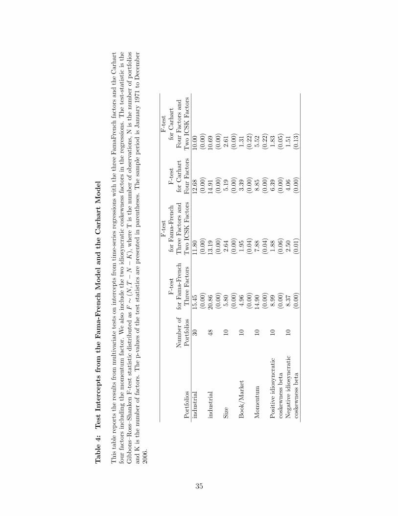
Tab
le4:
Tes
tIn
terc
epts
from
the
Fam
a-Fre
nch
Model
and
the
Car
har
tM
odel
Thi
sta
ble
repo
rts
the
resu
lts
from
mul
tiva
riat
ete
sts
onin
terc
epts
from
tim
e-se
ries
regr
essi
ons
wit
hth
eth
ree
Fam
aFre
nch
fact
ors
and
the
Car
hart
four
fact
ors
incl
udin
gth
em
omen
tum
fact
or.
We
also
incl
ude
the
two
idio
sync
rati
cco
skew
ness
fact
ors
inth
ere
gres
sion
s.T
hete
st-s
tati
stic
isth
eG
ibbo
ns–R
oss–
Shan
ken
F-t
est
stat
isti
cdi
stri
bute
das
F∼
(N,T−
N−
K),
whe
reT
isth
enu
mbe
rof
obse
rvat
ions
,Nis
the
num
ber
ofpo
rtfo
lios
and
Kis
the
num
ber
offa
ctor
s.T
hep-
valu
esof
the
test
stat
isti
csar
epr
esen
ted
inpa
rent
hese
s.T
hesa
mpl
epe
riod
isJa
nuar
y19
71to
Dec
embe
r20
06.
F-t
est
F-t
est
F-t
est
for
Fam
a-Fr
ench
F-t
est
for
Car
hart
Num
ber
offo
rFa
ma-
Fren
chT
hree
Fact
ors
and
for
Car
hart
Four
Fact
ors
and
Por
tfol
ios
Por
tfol
ios
Thr
eeFa
ctor
sT
wo
ICSK
Fact
ors
Four
Fact
ors
Tw
oIC
SKFa
ctor
sin
dust
rial
3015
.45
11.8
012
.68
10.0
0(0
.00)
(0.0
0)(0
.00)
(0.0
0)in
dust
rial
4820
.86
13.1
914
.91
10.6
9(0
.00)
(0.0
0)(0
.00)
(0.0
0)Si
ze10
5.80
2.64
5.19
2.61
(0.0
0)(0
.00)
(0.0
0)(0
.00)
Boo
k/M
arke
t10
4.96
1.95
3.39
1.31
(0.0
0)(0
.04)
(0.0
0)(0
.22)
Mom
entu
m10
14.9
07.
888.
855.
52(0
.00)
(0.0
4)(0
.00)
(0.2
2)Pos
itiv
eid
iosy
ncra
tic
108.
991.
886.
391.
83co
skew
ness
beta
(0.0
0)(0
.06)
(0.0
0)(0
.05)
Neg
ativ
eid
iosy
ncra
tic
108.
372.
504.
061.
51co
skew
ness
beta
(0.0
0)(0
.01)
(0.0
0)(0
.13)
35
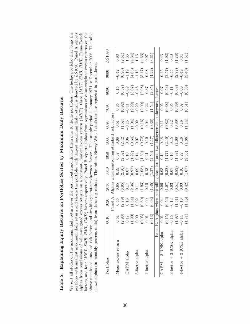
Tab
le5:
Expla
inin
gEquity
Ret
urn
son
Por
tfol
ios
Sor
ted
by
Max
imum
Dai
lyR
eturn
s
We
sort
alls
tock
son
the
max
imum
daily
retu
rnov
erth
epa
stm
onth
and
divi
deth
emin
to10
deci
lepo
rtfo
lios.
The
hedg
epo
rtfo
lioth
atlo
ngs
the
port
folio
wit
hsm
alle
stm
axim
umda
ilyre
turn
and
shor
tsth
epo
rtfo
liow
ith
larg
est
max
imum
daily
retu
rnis
deno
ted
byL
S10
90.
Pan
elA
repo
rts
alph
asfr
omre
gres
sion
sof
valu
e-w
eigh
ted
exce
ssre
turn
son
aco
nsta
nt,
mar
ket
exce
ssre
turn
(MK
T),
thre
e(M
KT
,SM
B,
HM
L)
Fam
a-Fr
ench
fact
ors,
and
four
(MK
T,SM
B,H
ML,U
MD
)fa
ctor
sre
spec
tive
ly.
Pan
elB
repo
rts
alph
asfr
omre
gres
sion
sof
valu
e-w
eigh
ted
exce
ssre
turn
son
the
abov
em
enti
oned
stan
dard
risk
fact
ors
and
two
idio
sync
rati
cco
skew
ness
fact
ors.
The
sam
ple
peri
odis
Janu
ary
1971
toD
ecem
ber
2006
.T
heta
ble
show
sal
phas
(in
mon
thly
perc
ent
unit
s)fr
omth
ese
regr
essi
ons.
The
robu
stN
ewey
-Wes
tt-
stat
isti
csar
ere
port
edin
pare
nthe
ses.
Por
tfol
ios
0010
1020
2030
3040
4050
5060
6070
7080
8090
9000
LS
1090
Pan
elA
.A
lpha
sw
hen
cont
rolli
ngst
anda
rdri
skfa
ctor
sM
ean
exce
ssre
turn
0.51
0.55
0.65
0.59
0.67
0.68
0.51
0.35
0.15
−0.4
20.
93(2
.93)
(2.7
9)(3
.05)
(2.5
6)(2
.62)
(2.4
2)(1
.57)
(0.9
2)(0
.37)
(0.9
6)(2
.51)
CA
PM
alph
a0.
170.
130.
170.
070.
100.
06−0
.15
−0.4
1−0
.62
−1.1
91.
36(1
.90)
(1.6
4)(2
.36)
(0.9
7)(1
.22)
(0.6
4)(1
.04)
(2.2
9)(3
.07)
(4.6
5)(4
.34)
3-fa
ctor
alph
a0.
000.
020.
110.
090.
140.
07−0
.02
−0.2
9−0
.48
−1.1
51.
15(0
.05)
(0.3
0)(1
.93)
(1.0
8)(1
.69)
(0.7
2)(0
.16)
(2.0
0)(2
.98)
(5.4
7)(4
.66)
4-fa
ctor
alph
a−0
.01
−0.0
00.
100.
130.
210.
100.
04−0
.22
−0.3
7−0
.98
0.97
(0.1
3)(0
.03)
(1.4
5)(1
.27)
(2.5
0)(1
.17)
(0.3
6)(1
.54)
(2.3
5)(4
.22)
(3.6
1)Pan
elB
.A
lpha
sw
hen
cont
rolli
ngst
anda
rdan
dtw
oid
iosy
ncra
tic
cosk
ewne
ssfa
ctor
sC
AP
M+
2IC
SKal
pha
−0.0
1−0
.04
0.06
0.03
0.14
0.18
0.11
0.05
−0.0
7−0
.45
0.43
(0.1
5)(0
.56)
(1.0
7)(0
.32)
(1.7
7)(2
.10)
(0.8
2)(0
.38)
(0.5
3)(2
.57)
(1.9
2)3-
fact
or+
2IC
SKal
pha
−0.1
5−0
.13
0.03
0.07
0.16
0.15
0.12
0.05
−0.1
1−0
.55
0.40
(1.9
7)(1
.51)
(0.5
1)(0
.83)
(1.8
8)(1
.60)
(0.8
0)(0
.39)
(0.6
8)(2
.77)
(1.7
8)4-
fact
or+
2IC
SKal
pha
−0.1
4−0
.13
0.03
0.10
0.22
0.18
0.16
0.07
−0.0
6−0
.49
0.34
(1.7
1)(1
.46)
(0.4
2)(1
.07)
(2.5
5)(1
.88)
(1.1
4)(0
.51)
(0.3
8)(2
.40)
(1.5
1)
36

Table 6: Predictive Performance of Merton’s Model
This table reports the number of bankruptcy and performance delistings as a function of default risk rankbased on Merton’s model. At the end of each month firms are assigned into portfolios according to theirprobability of default measures. We construct 10 portfolios containing stocks in percentiles 0-5, 5-10,10-20, 20-40, 40-60, 60-80, 80-90, 90-95, 95-99, and 99-100 of the distribution of the default measure.Portfolio 1 contains firms with the lowest default probability measure. BD is the number of bankruptcyand liquidation delistings, and PD is the number of performance delistings. The sample period is January1971 to December 2006.
Number of Number ofBankruptcy Delistings Performance Delistings
Portfolio (BD) (PD)1 0 22 0 33 1 114 0 235 1 276 2 427 3 558 7 679 20 11110 26 102
37

Table 7: Summary Statistics of Returns on Distress-Sorted Portfolios
This table reports the mean, standard deviation, skewness, and kurtosis of monthly returns, in percentagepoints, on ten distress-sorted portfolios. It also reports unconditional coskewness betas, idiosyncraticcoskewness betas, and idiosyncratic skewness of the ten portfolios, as well as the average size, in milliondollars, of firms in each portfolio. At the end of each month firms are assigned into portfolios accordingto their probability of default measures. We construct 10 portfolios containing stocks in percentiles 0-5,5-10, 10-20, 20-40, 40-60, 60-80, 80-90, 90-95, 95-99, and 99-100 of the distribution of the default measure.Portfolio 1 contains firms with the lowest default probability measure. Value-weighted realized returnsin the next month are calculated for the ten portfolios. The sample period is January 1971 to December2006.
0005 0510 1020 2040 4060 6080 8090 9095 9599 9900Mean 0.92 0.98 1.17 1.03 1.01 0.88 0.81 0.36 0.41 −0.51Stdev 4.48 4.40 4.36 4.87 5.81 6.57 7.64 9.02 10.70 14.96Skew −0.29 −0.48 −0.16 −0.37 −0.41 −0.27 0.15 0.49 0.86 0.81Kurt 5.42 4.94 4.65 5.53 5.28 5.13 7.53 9.82 13.36 7.65Coskew(10−4) 0.31 −0.69 1.69 0.05 −0.95 −1.60 −1.70 −2.84 −2.89 0.76Idio. Coskew(10−2) 0.01 0.00 0.00 0.00 0.01 0.04 0.09 0.22 0.30 0.65Idio. Skew −0.26 −0.41 0.21 0.48 0.16 0.34 1.05 1.01 1.71 0.95Mean size 4.90 4.33 2.80 1.43 0.71 0.35 0.18 0.11 0.10 0.07
38
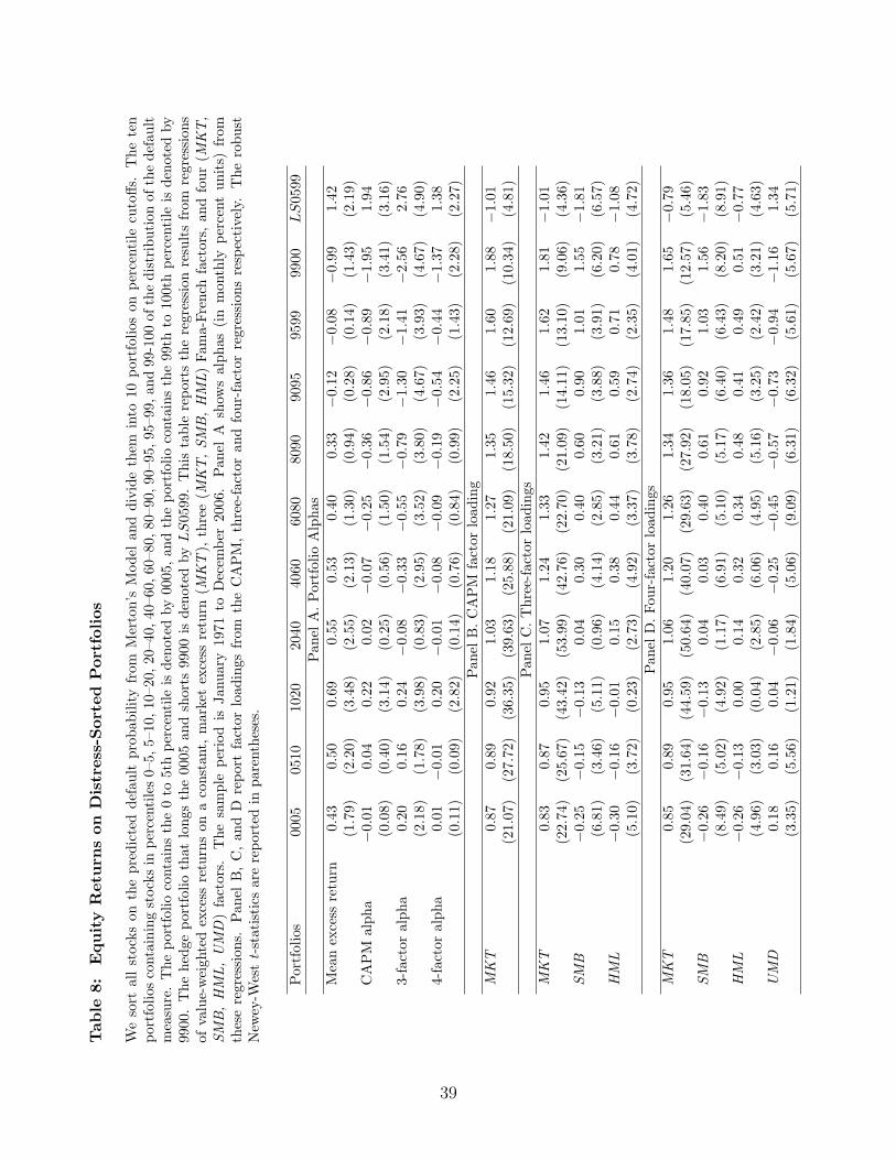
Tab
le8:
Equity
Ret
urn
son
Dis
tres
s-Sor
ted
Por
tfol
ios
We
sort
all
stoc
kson
the
pred
icte
dde
faul
tpr
obab
ility
from
Mer
ton’
sM
odel
and
divi
deth
emin
to10
port
folio
son
perc
enti
lecu
toffs
.T
hete
npo
rtfo
lios
cont
aini
ngst
ocks
inpe
rcen
tile
s0–
5,5–
10,1
0–20
,20–
40,4
0–60
,60–
80,8
0–90
,90–
95,9
5–99
,and
99-1
00of
the
dist
ribu
tion
ofth
ede
faul
tm
easu
re.
The
port
folio
cont
ains
the
0to
5th
perc
enti
leis
deno
ted
by00
05,an
dth
epo
rtfo
lioco
ntai
nsth
e99
thto
100t
hpe
rcen
tile
isde
note
dby
9900
.T
hehe
dge
port
folio
that
long
sth
e00
05an
dsh
orts
9900
isde
note
dby
LS
0599
.T
his
tabl
ere
port
sth
ere
gres
sion
resu
lts
from
regr
essi
ons
ofva
lue-
wei
ghte
dex
cess
retu
rns
ona
cons
tant
,m
arke
tex
cess
retu
rn(M
KT
),th
ree
(MK
T,SM
B,H
ML)
Fam
a-Fr
ench
fact
ors,
and
four
(MK
T,
SMB,
HM
L,
UM
D)
fact
ors.
The
sam
ple
peri
odis
Janu
ary
1971
toD
ecem
ber
2006
.Pan
elA
show
sal
phas
(in
mon
thly
perc
ent
unit
s)fr
omth
ese
regr
essi
ons.
Pan
elB
,C
,an
dD
repo
rtfa
ctor
load
ings
from
the
CA
PM
,th
ree-
fact
oran
dfo
ur-fac
tor
regr
essi
ons
resp
ecti
vely
.T
hero
bust
New
ey-W
est
t-st
atis
tics
are
repo
rted
inpa
rent
hese
s.
Por
tfol
ios
0005
0510
1020
2040
4060
6080
8090
9095
9599
9900
LS
0599
Pan
elA
.Por
tfol
ioA
lpha
sM
ean
exce
ssre
turn
0.43
0.50
0.69
0.55
0.53
0.40
0.33
−0.1
2−0
.08
−0.9
91.
42(1
.79)
(2.2
0)(3
.48)
(2.5
5)(2
.13)
(1.3
0)(0
.94)
(0.2
8)(0
.14)
(1.4
3)(2
.19)
CA
PM
alph
a−0
.01
0.04
0.22
0.02
−0.0
7−0
.25
−0.3
6−0
.86
−0.8
9−1
.95
1.94
(0.0
8)(0
.40)
(3.1
4)(0
.25)
(0.5
6)(1
.50)
(1.5
4)(2
.95)
(2.1
8)(3
.41)
(3.1
6)3-
fact
oral
pha
0.20
0.16
0.24
−0.0
8−0
.33
−0.5
5−0
.79
−1.3
0−1
.41
−2.5
62.
76(2
.18)
(1.7
8)(3
.98)
(0.8
3)(2
.95)
(3.5
2)(3
.80)
(4.6
7)(3
.93)
(4.6
7)(4
.90)
4-fa
ctor
alph
a0.
01−0
.01
0.20
−0.0
1−0
.08
−0.0
9−0
.19
−0.5
4−0
.44
−1.3
71.
38(0
.11)
(0.0
9)(2
.82)
(0.1
4)(0
.76)
(0.8
4)(0
.99)
(2.2
5)(1
.43)
(2.2
8)(2
.27)
Pan
elB
.C
AP
Mfa
ctor
load
ing
MK
T0.
870.
890.
921.
031.
181.
271.
351.
461.
601.
88−1
.01
(21.
07)
(27.
72)
(36.
35)
(39.
63)
(25.
88)
(21.
09)
(18.
50)
(15.
32)
(12.
69)
(10.
34)
(4.8
1)Pan
elC
.T
hree
-fac
tor
load
ings
MK
T0.
830.
870.
951.
071.
241.
331.
421.
461.
621.
81−1
.01
(22.
74)
(25.
67)
(43.
42)
(53.
99)
(42.
76)
(22.
70)
(21.
09)
(14.
11)
(13.
10)
(9.0
6)(4
.36)
SMB
−0.2
5−0
.15
−0.1
30.
040.
300.
400.
600.
901.
011.
55−1
.81
(6.8
1)(3
.46)
(5.1
1)(0
.96)
(4.1
4)(2
.85)
(3.2
1)(3
.88)
(3.9
1)(6
.20)
(6.5
7)H
ML
−0.3
0−0
.16
−0.0
10.
150.
380.
440.
610.
590.
710.
78−1
.08
(5.1
0)(3
.72)
(0.2
3)(2
.73)
(4.9
2)(3
.37)
(3.7
8)(2
.74)
(2.3
5)(4
.01)
(4.7
2)Pan
elD
.Fo
ur-fac
tor
load
ings
MK
T0.
850.
890.
951.
061.
201.
261.
341.
361.
481.
65−0
.79
(29.
04)
(31.
64)
(44.
59)
(50.
64)
(40.
07)
(29.
63)
(27.
92)
(18.
05)
(17.
85)
(12.
57)
(5.4
6)SM
B−0
.26
−0.1
6−0
.13
0.04
0.03
0.40
0.61
0.92
1.03
1.56
−1.8
3(8
.49)
(5.0
2)(4
.92)
(1.1
7)(6
.91)
(5.1
0)(5
.17)
(6.4
0)(6
.43)
(8.2
0)(8
.91)
HM
L−0
.26
−0.1
30.
000.
140.
320.
340.
480.
410.
490.
51−0
.77
(4.9
6)(3
.03)
(0.0
4)(2
.85)
(6.0
6)(4
.95)
(5.1
6)(3
.25)
(2.4
2)(3
.21)
(4.6
3)U
MD
0.18
0.16
0.04
−0.0
6−0
.25
−0.4
5−0
.57
−0.7
3−0
.94
−1.1
61.
34(3
.35)
(5.5
6)(1
.21)
(1.8
4)(5
.06)
(9.0
9)(6
.31)
(6.3
2)(5
.61)
(5.6
7)(5
.71)
39
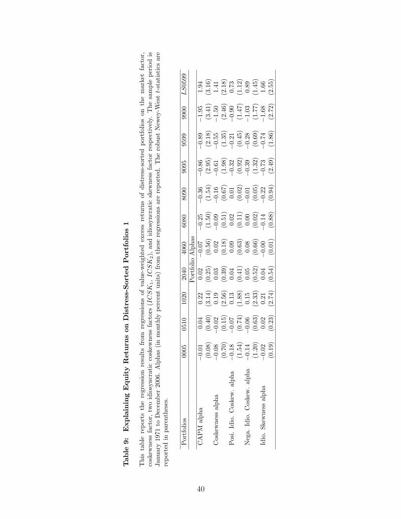
Tab
le9:
Expla
inin
gEquity
Ret
urn
son
Dis
tres
s-Sor
ted
Por
tfol
ios
1
Thi
sta
ble
repo
rts
the
regr
essi
onre
sult
sfr
omre
gres
sion
sof
valu
e-w
eigh
ted
exce
ssre
turn
sof
dist
ress
-sor
ted
port
folio
son
the
mar
ket
fact
or,
cosk
ewne
ssfa
ctor
,tw
oid
iosy
ncra
tic
cosk
ewne
ssfa
ctor
s(I
CS
K1,
IC
SK
2),
and
idio
sync
rati
csk
ewne
ssfa
ctor
resp
ecti
vely
.T
hesa
mpl
epe
riod
isJa
nuar
y19
71to
Dec
embe
r20
06.
Alp
has
(in
mon
thly
perc
ent
unit
s)fr
omth
ese
regr
essi
ons
are
repo
rted
.T
hero
bust
New
ey-W
est
t-st
atis
tics
are
repo
rted
inpa
rent
hese
s.
Por
tfol
ios
0005
0510
1020
2040
4060
6080
8090
9095
9599
9900
LS
0599
Por
tfol
ioA
lpha
sC
AP
Mal
pha
−0.0
10.
040.
220.
02−0
.07
−0.2
5−0
.36
−0.8
6−0
.89
−1.9
51.
94(0
.08)
(0.4
0)(3
.14)
(0.2
5)(0
.56)
(1.5
0)(1
.54)
(2.9
5)(2
.18)
(3.4
1)(3
.16)
Cos
kew
ness
alph
a−0
.08
−0.0
20.
190.
030.
02−0
.09
−0.1
6−0
.61
−0.5
5−1
.50
1.41
(0.7
0)(0
.15)
(2.5
6)(0
.39)
(0.1
8)(0
.51)
(0.6
7)(1
.98)
(1.3
5)(2
.46)
(2.1
8)Pos
i.Id
io.
Cos
kew
.al
pha
−0.1
8−0
.07
0.13
0.04
0.09
0.02
0.01
−0.3
2−0
.21
−0.9
00.
73(1
.54)
(0.7
4)(1
.88)
(0.4
1)(0
.63)
(0.1
1)(0
.02)
(0.9
2)(0
.45)
(1.4
7)(1
.12)
Neg
a.Id
io.
Cos
kew
.al
pha
−0.1
4−0
.06
0.15
0.05
0.08
0.00
−0.0
1−0
.39
−0.2
8−1
.03
0.89
(1.2
0)(0
.63)
(2.3
3)(0
.52)
(0.6
6)(0
.02)
(0.0
5)(1
.32)
(0.6
9)(1
.77)
(1.4
5)Id
io.
Skew
ness
alph
a−0
.02
0.02
0.21
0.04
−0.0
0−0
.14
−0.2
2−0
.73
−0.7
4−1
.68
1.66
(0.1
9)(0
.23)
(2.7
4)(0
.54)
(0.0
1)(0
.88)
(0.9
4)(2
.49)
(1.8
6)(2
.72)
(2.5
5)
40
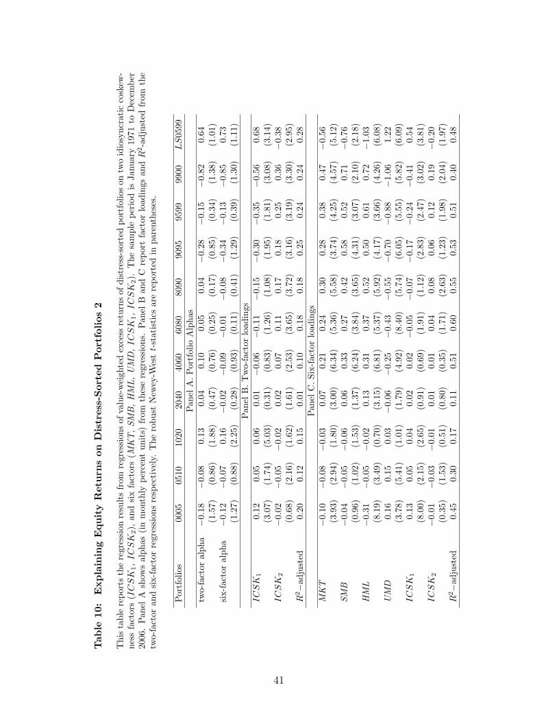
Tab
le10
:Expla
inin
gEquity
Ret
urn
son
Dis
tres
s-Sor
ted
Por
tfol
ios
2
Thi
sta
ble
repo
rts
the
regr
essi
onre
sult
sfr
omre
gres
sion
sof
valu
e-w
eigh
ted
exce
ssre
turn
sof
dist
ress
-sor
ted
port
folio
son
two
idio
sync
rati
cco
skew
-ne
ssfa
ctor
s(I
CS
K1,
IC
SK
2),
and
six
fact
ors
(MK
T,SM
B,H
ML,U
MD
,IC
SK
1,
IC
SK
2).
The
sam
ple
peri
odis
Janu
ary
1971
toD
ecem
ber
2006
.Pan
elA
show
sal
phas
(in
mon
thly
perc
ent
unit
s)fr
omth
ese
regr
essi
ons.
Pan
elB
and
Cre
port
fact
orlo
adin
gsan
dR
2-a
djus
ted
from
the
two-
fact
oran
dsi
x-fa
ctor
regr
essi
ons
resp
ecti
vely
.T
hero
bust
New
ey-W
est
t-st
atis
tics
are
repo
rted
inpa
rent
hese
s.
Por
tfol
ios
0005
0510
1020
2040
4060
6080
8090
9095
9599
9900
LS
0599
Pan
elA
.Por
tfol
ioA
lpha
stw
o-fa
ctor
alph
a−0
.18
−0.0
80.
130.
040.
100.
050.
04−0
.28
−0.1
5−0
.82
0.64
(1.5
7)(0
.86)
(1.8
8)(0
.47)
(0.7
6)(0
.25)
(0.1
7)(0
.85)
(0.3
4)(1
.38)
(1.0
1)si
x-fa
ctor
alph
a−0
.12
−0.0
70.
16−0
.02
−0.0
9−0
.01
−0.0
8−0
.34
−0.1
3−0
.85
0.73
(1.2
7)(0
.88)
(2.2
5)(0
.28)
(0.9
3)(0
.11)
(0.4
1)(1
.29)
(0.3
9)(1
.30)
(1.1
1)Pan
elB
.T
wo-
fact
orlo
adin
gsIC
SK
10.
120.
050.
060.
01−0
.06
−0.1
1−0
.15
−0.3
0−0
.35
−0.5
60.
68(3
.07)
(1.7
4)(5
.03)
(0.3
1)(0
.83)
(1.2
6)(1
.08)
(1.9
5)(1
.81)
(3.0
8)(3
.14)
IC
SK
2−0
.02
−0.0
5−0
.02
0.02
0.07
0.11
0.17
0.18
0.25
0.36
−0.3
8(0
.68)
(2.1
6)(1
.62)
(1.6
1)(2
.53)
(3.6
5)(3
.72)
(3.1
6)(3
.19)
(3.3
0)(2
.95)
R2−a
djus
ted
0.20
0.12
0.15
0.01
0.10
0.18
0.18
0.25
0.24
0.24
0.28
Pan
elC
.Si
x-fa
ctor
load
ings
MK
T−0
.10
−0.0
8−0
.03
0.07
0.21
0.24
0.30
0.28
0.38
0.47
−0.5
6(3
.93)
(2.9
4)(1
.80)
(3.0
0)(6
.34)
(5.3
6)(5
.58)
(3.7
4)(4
.25)
(4.5
7)(5
.12)
SMB
−0.0
4−0
.05
−0.0
60.
060.
330.
270.
420.
580.
520.
71−0
.76
(0.9
6)(1
.02)
(1.5
3)(1
.37)
(6.2
4)(3
.84)
(3.6
5)(4
.31)
(3.0
7)(2
.10)
(2.1
8)H
ML
−0.3
1−0
.05
−0.0
20.
130.
310.
370.
520.
500.
610.
72−1
.03
(8.1
9)(3
.49)
(0.7
0)(3
.15)
(6.8
1)(5
.37)
(5.9
2)(4
.17)
(3.6
6)(4
.26)
(6.0
8)U
MD
0.16
0.15
0.03
−0.0
6−0
.25
−0.4
3−0
.55
−0.7
0−0
.88
−1.0
61.
22(3
.78)
(5.4
1)(1
.01)
(1.7
9)(4
.92)
(8.4
0)(5
.74)
(6.0
5)(5
.55)
(5.8
2)(6
.09)
IC
SK
10.
130.
050.
040.
020.
02−0
.05
−0.0
7−0
.17
−0.2
4−0
.41
0.54
(8.0
0)(2
.15)
(2.6
5)(0
.91)
(0.6
9)(1
.91)
(1.1
2)(2
.83)
(2.4
7)(3
.02)
(3.8
1)IC
SK
2−0
.01
−0.0
3−0
.01
0.01
0.01
0.04
0.08
0.06
0.12
0.19
−0.2
0(0
.35)
(1.5
3)(0
.51)
(0.8
0)(0
.35)
(1.7
1)(2
.63)
(1.2
3)(1
.98)
(2.0
4)(1
.97)
R2−a
djus
ted
0.45
0.30
0.17
0.11
0.51
0.60
0.55
0.53
0.51
0.40
0.48
41
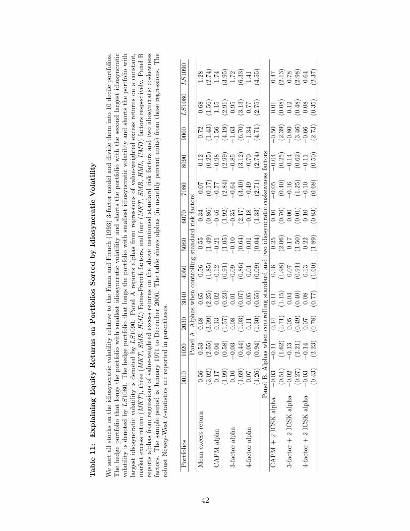
Tab
le11
:Expla
inin
gEquity
Ret
urn
son
Por
tfol
ios
Sor
ted
by
Idio
syncr
atic
Vol
atility
We
sort
alls
tock
son
the
idio
sync
rati
cvo
lati
lity
rela
tive
toth
eFa
ma
and
Fren
ch(1
993)
3-fa
ctor
mod
elan
ddi
vide
them
into
10de
cile
port
folio
s.T
hehe
dge
port
folio
that
long
sth
epo
rtfo
liow
ith
smal
lest
idio
sync
rati
cvo
lati
lity
and
shor
tsth
epo
rtfo
liow
ith
the
seco
ndla
rges
tid
iosy
ncra
tic
vola
tilit
yis
deno
ted
byL
S10
80.
The
hedg
epo
rtfo
lioth
atlo
ngs
the
port
folio
wit
hsm
alle
stid
iosy
ncra
tic
vola
tilit
yan
dsh
orts
the
port
folio
wit
hla
rges
tid
iosy
ncra
tic
vola
tilit
yis
deno
ted
byL
S10
90.
Pan
elA
repo
rts
alph
asfr
omre
gres
sion
sof
valu
e-w
eigh
ted
exce
ssre
turn
son
aco
nsta
nt,
mar
ket
exce
ssre
turn
(MK
T),
thre
e(M
KT
,SM
B,H
ML)
Fam
a-Fr
ench
fact
ors,
and
four
(MK
T,SM
B,H
ML,U
MD
)fa
ctor
sre
spec
tive
ly.
Pan
elB
repo
rts
alph
asfr
omre
gres
sion
sof
valu
e-w
eigh
ted
exce
ssre
turn
son
the
abov
em
enti
oned
stan
dard
risk
fact
ors
and
two
idio
sync
rati
cco
skew
ness
fact
ors.
The
sam
ple
peri
odis
Janu
ary
1971
toD
ecem
ber
2006
.T
heta
ble
show
sal
phas
(in
mon
thly
perc
ent
unit
s)fr
omth
ese
regr
essi
ons.
The
robu
stN
ewey
-Wes
tt-
stat
isti
csar
ere
port
edin
pare
nthe
ses.
Por
tfol
ios
0010
1020
2030
3040
4050
5060
6070
7080
8090
9000
LS
1080
LS
1090
Pan
elA
.A
lpha
sw
hen
cont
rolli
ngst
anda
rdri
skfa
ctor
sM
ean
exce
ssre
turn
0.56
0.53
0.68
0.65
0.56
0.55
0.34
0.07
−0.1
2−0
.72
0.68
1.28
(3.0
2)(2
.55)
(3.0
9)(2
.25)
(1.8
5)(1
.49)
(0.8
6)(0
.17)
(0.2
5)(1
.43)
(1.5
6)(2
.74)
CA
PM
alph
a0.
170.
040.
130.
02−0
.12
−0.2
1−0
.46
−0.7
7−0
.98
−1.5
61.
151.
74(1
.99)
(0.5
8)(1
.57)
(0.2
3)(0
.91)
(1.0
5)(1
.92)
(2.8
4)(2
.99)
(4.1
9)(2
.91)
(3.9
5)3-
fact
oral
pha
0.10
−0.0
30.
080.
01−0
.09
−0.1
0−0
.35
−0.6
4−0
.85
−1.6
30.
951.
72(1
.69)
(0.4
4)(1
.03)
(0.0
7)(0
.86)
(0.6
4)(2
.17)
(3.4
0)(3
.12)
(6.7
0)(3
.13)
(6.3
3)4-
fact
oral
pha
0.07
−0.0
50.
110.
050.
01−0
.01
−0.1
8−0
.49
−0.7
0−1
.34
0.77
1.41
(1.2
6)(0
.94)
(1.3
0)(0
.55)
(0.0
9)(0
.04)
(1.3
3)(2
.71)
(2.7
4)(4
.71)
(2.7
5)(4
.55)
Pan
elB
.A
lpha
sw
hen
cont
rolli
ngst
anda
rdan
dtw
oid
iosy
ncra
tic
cosk
ewne
ssfa
ctor
sC
AP
M+
2IC
SKal
pha
−0.0
3−0
.11
0.14
0.11
0.16
0.25
0.10
−0.0
5−0
.04
−0.5
00.
010.
47(0
.51)
(1.6
2)(1
.71)
(1.1
5)(1
.98)
(2.0
6)(0
.76)
(0.4
0)(0
.25)
(2.3
9)(0
.08)
(2.1
3)3-
fact
or+
2IC
SKal
pha
−0.0
2−0
.13
0.05
0.04
0.07
0.17
0.00
−0.1
6−0
.14
−0.8
00.
120.
78(0
.27)
(2.2
1)(0
.49)
(0.4
0)(0
.91)
(1.5
0)(0
.01)
(1.2
5)(0
.62)
(3.4
6)(0
.48)
(2.9
8)4-
fact
or+
2IC
SKal
pha
−0.0
3−0
.14
0.07
0.08
0.13
0.22
0.10
−0.1
0−0
.11
−0.6
60.
080.
64(0
.43)
(2.2
3)(0
.78)
(0.7
7)(1
.60)
(1.8
9)(0
.83)
(0.6
8)(0
.50)
(2.7
3)(0
.35)
(2.3
7)
42
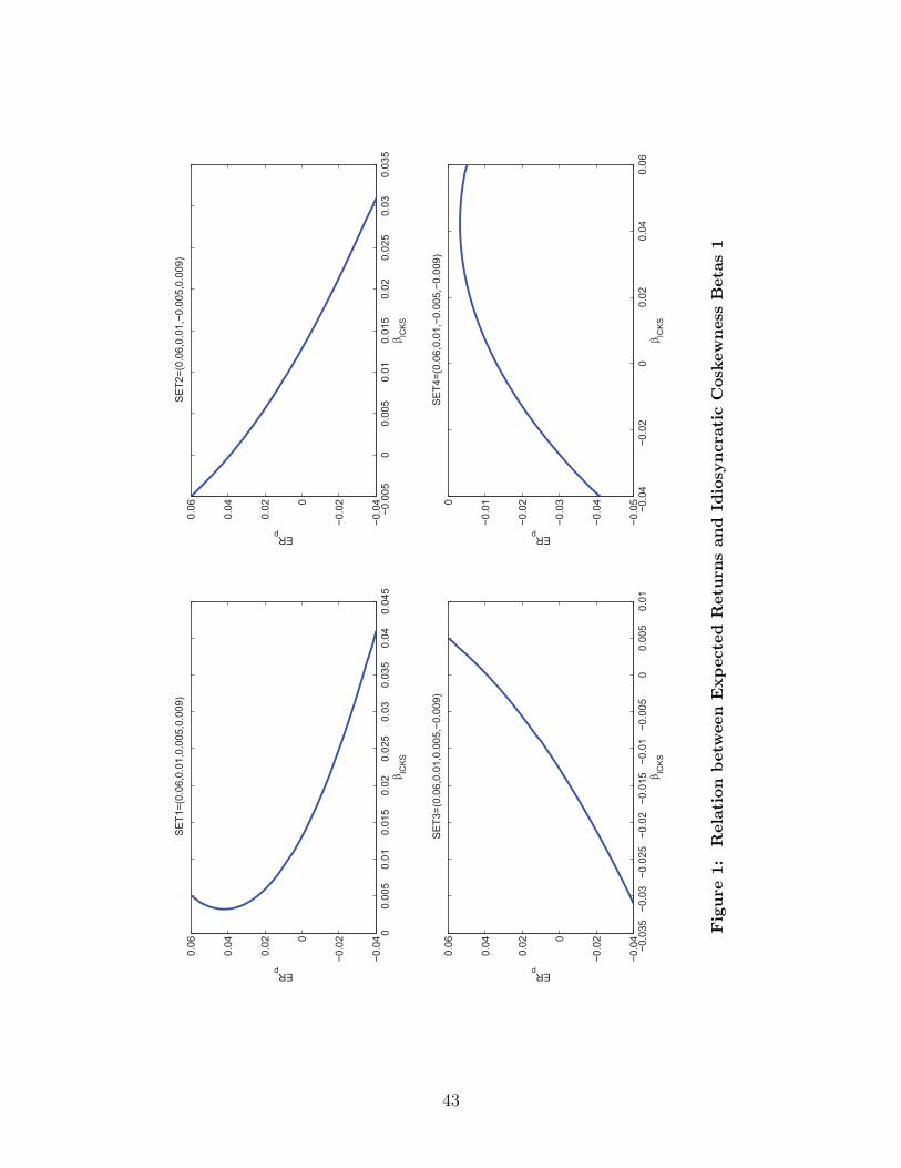
00.005
0.01
0.015
0.02
0.025
0.03
0.035
0.04
0.045
−0.04
−0.020
0.02
0.04
0.06
βICKS
ERp
SET1=(0.06,0.01,0.005,0.009)
−0.005
00.005
0.01
0.015
0.02
0.025
0.03
0.035
−0.04
−0.020
0.02
0.04
0.06
βICKS
ERp
SET2=(0.06,0.01,−0.005,0.009)
−0.035
−0.03
−0.025
−0.02
−0.015
−0.01
−0.005
00.005
0.01
−0.04
−0.020
0.02
0.04
0.06
βICKS
ERp
SET3=(0.06,0.01,0.005,−0.009)
−0.04
−0.02
00.02
0.04
0.06
−0.05
−0.04
−0.03
−0.02
−0.010
βICKS
ERp
SET4=(0.06,0.01,−0.005,−0.009)
Fig
ure
1:R
elat
ion
bet
wee
nExpec
ted
Ret
urn
san
dId
iosy
ncr
atic
Cos
kew
nes
sB
etas
1
43
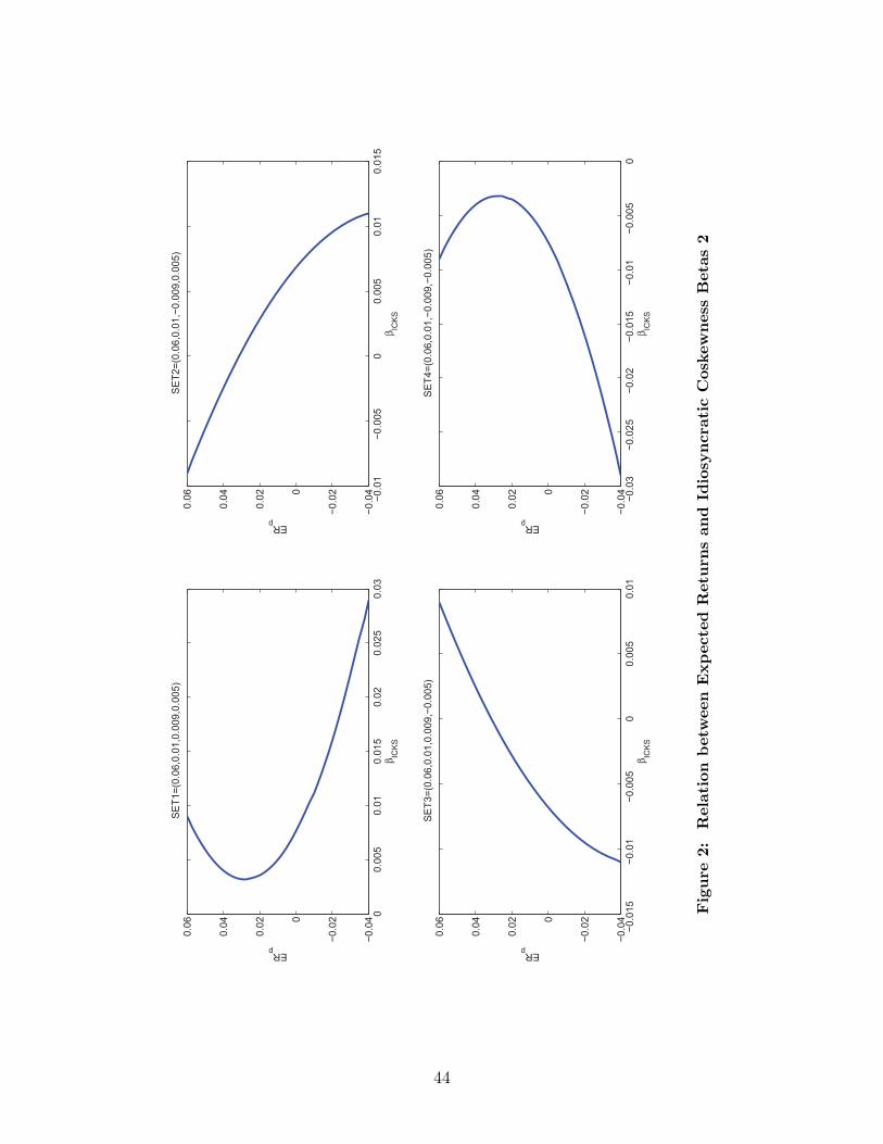
00.005
0.01
0.015
0.02
0.025
0.03
−0.04
−0.020
0.02
0.04
0.06
βICKS
ERp
SET1=(0.06,0.01,0.009,0.005)
−0.01
−0.005
00.005
0.01
0.015
−0.04
−0.020
0.02
0.04
0.06
βICKS
ERp
SET2=(0.06,0.01,−0.009,0.005)
−0.015
−0.01
−0.005
00.005
0.01
−0.04
−0.020
0.02
0.04
0.06
βICKS
ERp
SET3=(0.06,0.01,0.009,−0.005)
−0.03
−0.025
−0.02
−0.015
−0.01
−0.005
0−0.04
−0.020
0.02
0.04
0.06
βICKS
ERp
SET4=(0.06,0.01,−0.009,−0.005)
Fig
ure
2:R
elat
ion
bet
wee
nExpec
ted
Ret
urn
san
dId
iosy
ncr
atic
Cos
kew
nes
sB
etas
2
44
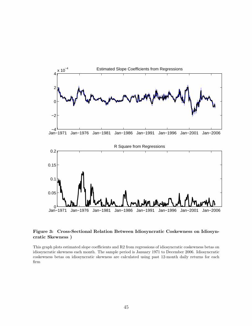
Jan−1971 Jan−1976 Jan−1981 Jan−1986 Jan−1991 Jan−1996 Jan−2001 Jan−2006−4
−2
0
2
4x 10
−4 Estimated Slope Coefficients from Regressions
Jan−1971 Jan−1976 Jan−1981 Jan−1986 Jan−1991 Jan−1996 Jan−2001 Jan−20060
0.05
0.1
0.15
0.2R Square from Regressions
Figure 3: Cross-Sectional Relation Between Idiosyncratic Coskewness on Idiosyn-cratic Skewness )
This graph plots estimated slope coefficients and R2 from regressions of idiosyncratic coskewness betas onidiosyncratic skewness each month. The sample period is January 1971 to December 2006. Idiosyncraticcoskewness betas on idiosyncratic skewness are calculated using past 12-month daily returns for eachfirm
45
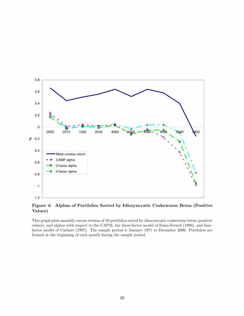
-1.2
-1
-0.8
-0.6
-0.4
-0.2
0
0.2
0.4
0.6
0.8
0005 0510 1020 2040 4060 6080 8090 9095 9599 9900
%
Mean excess return
CAMP alpha
3-factor alpha
4-factor alpha
Figure 4: Alphas of Portfolios Sorted by Idiosyncratic Coskewness Betas (PositiveValues)
This graph plots monthly excess returns of 10 portfolios sorted by idiosyncratic coskewness betas (positivevalues), and alphas with respect to the CAPM, the three-factor model of Fama-French (1993), and four-factor model of Carhart (1997). The sample period is January 1971 to December 2006. Portfolios areformed at the beginning of each month during the sample period.
46
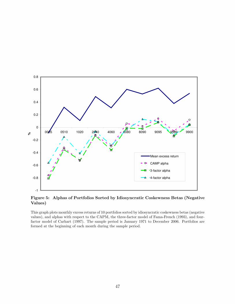
-1
-0.8
-0.6
-0.4
-0.2
0
0.2
0.4
0.6
0.8
0005 0510 1020 2040 4060 6080 8090 9095 9599 9900
%
Mean excess return
CAMP alpha
3-factor alpha
4-factor alpha
Figure 5: Alphas of Portfolios Sorted by Idiosyncratic Coskewness Betas (NegativeValues)
This graph plots monthly excess returns of 10 portfolios sorted by idiosyncratic coskewness betas (negativevalues), and alphas with respect to the CAPM, the three-factor model of Fama-French (1993), and four-factor model of Carhart (1997). The sample period is January 1971 to December 2006. Portfolios areformed at the beginning of each month during the sample period.
47
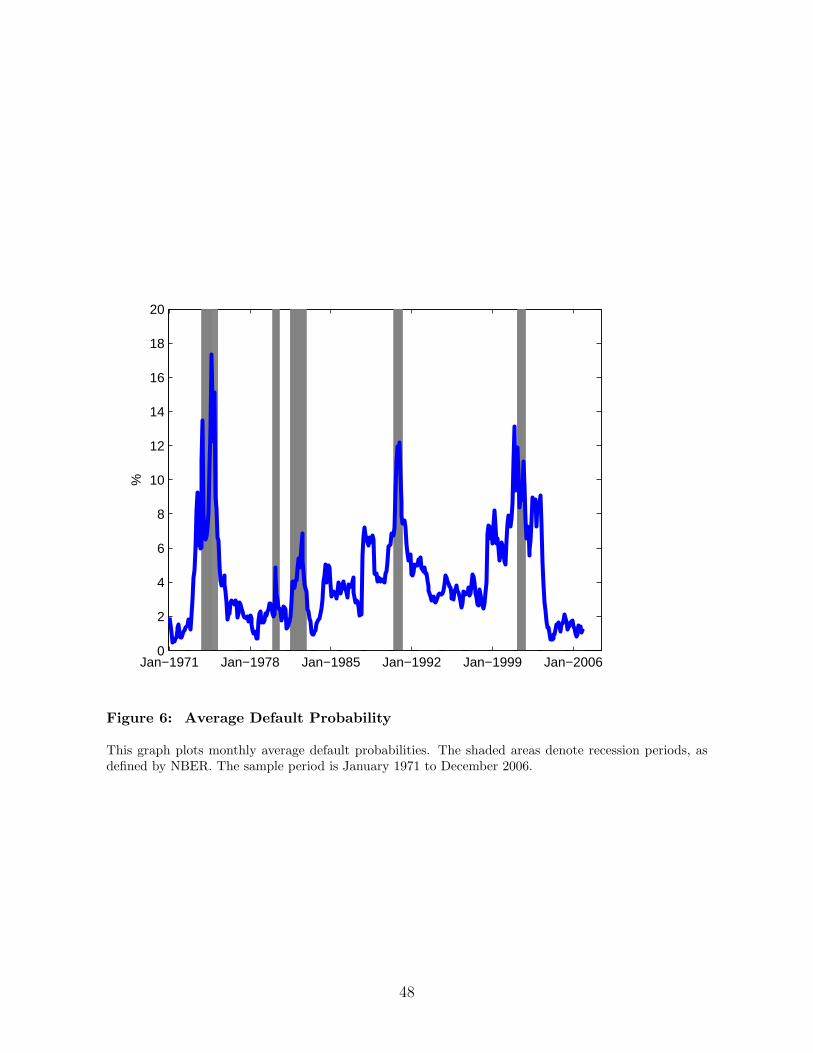
Jan−1971 Jan−1978 Jan−1985 Jan−1992 Jan−1999 Jan−20060
2
4
6
8
10
12
14
16
18
20
%
Figure 6: Average Default Probability
This graph plots monthly average default probabilities. The shaded areas denote recession periods, asdefined by NBER. The sample period is January 1971 to December 2006.
48
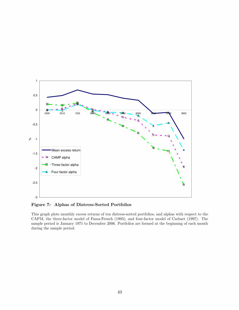
-3
-2.5
-2
-1.5
-1
-0.5
0
0.5
1
0005 0510 1020 2040 4060 6080 8090 9095 9599 9900
%
Mean excess return
CAMP alpha
Three-factor alpha
Four-factor alpha
Figure 7: Alphas of Distress-Sorted Portfolios
This graph plots monthly excess returns of ten distress-sorted portfolios, and alphas with respect to theCAPM, the three-factor model of Fama-French (1993), and four-factor model of Carhart (1997). Thesample period is January 1971 to December 2006. Portfolios are formed at the beginning of each monthduring the sample period.
49