growth and reproduction of female short-beaked … of san diego san diego growth and reproduction of...
TRANSCRIPT

UNIVERSITY OF SAN DIEGO
San Diego
Growth and reproduction of female short-beaked common dolphins, Delphinus delphis, in the eastern tropical Pacific
A thesis submitted in partial satisfaction of the requirements for the degree of
Master of Science in Marine Science
by Kerri Danil
Thesis Committee Susan J. Chivers, Ph.D., Chair
Hugh I. Ellis, Ph.D. William F. Perrin, Ph.D. Bonnie J. Ripley, Ph.D.

The thesis of Kerri Danil is approved by:
_______________________________________ Susan J. Chivers, Thesis Committee Chair
Southwest Fisheries Science Center
________________________________________ Hugh I. Ellis, Thesis Advisor
University of San Diego
________________________________________ William F. Perrin, Thesis Committee Member
Southwest Fisheries Science Center
_________________________________________ Bonnie J. Ripley, Thesis Committee Member
University of San Diego
University of San Diego
San Diego
2004
ii

Copyright 2004 Kerri Danil
iii
Acknowledgments
The development and completion of this thesis would not have been
possible without the help of many people, some of whom unknowingly began
working on this project the year after I was born! I thank the many fishery
observers who spent long days collecting data and samples in the field and Ruth
Miller who processed the incoming samples. Kelly Robertson and Mike Henshaw
aged the hundreds of teeth used in chapters three and four.
A big thank you to my committee: Susan, Hugh, Bill, and Bonnie. Your
ideas, guidance, and editing skills were much appreciated! And of course, to my
USD graduate student cohort: thanks for your input in the beginning stages of this
project.
Southwest Fisheries Science Center funded the entirety of this project and
provided a tremendous network of individuals who provided emotional and
scientific support. First and foremost, I’d like to thank my chair, Susan Chivers,
who balanced the roles of mentor, thesis chair, and supervisor amazingly well.
Her flexibility, patience, time, support, encouragement, and ideas were greatly
appreciated. Thank you Kelly Robertson for training/advising me on aging and
being willing to explore new aging techniques with me. Thank you Eric Archer
for your time and patience in answering my many statistical questions and for
programming the double phase growth model. Thanks to Lisa Ballance for her
insight into the ecology of the ETP that led my research in directions that I had
not foreseen. Steve Reilly kindly took time to talk to me about multivariate
statistics. Paul Fiedler provided oceanographic data and insight into the
iv

oceanographic trends of the ETP. Thank you, Jason Larese, for letting me use
your logistic bootstrap program and engaging me in conversations of life and life
history. Thank you Nick Kellar for being someone else who was excited about
and could see the great value of life history studies.
A huge thanks goes out to my family. Chris P., Mom, Risa, John, and
Chris I. provided the love, encouragement, and support to keep me sane during
these past few years. Thank you Chris P. for putting up with my times of absence
(emotional and physical), being the guinea pig for my presentations, and simply
listening when I needed to be heard.
v

TABLE OF CONTENTS
LIST OF TABLES................................................................................................. x
LIST OF FIGURES .............................................................................................. xii
CHAPTER 1: GENERAL INTRODUCTION ...................................................... 1
CHAPTER 2: LITERATURE REVIEW............................................................... 8
Odontocete life history strategy .............................................................................. 8
Age.......................................................................................................................... 9
Tooth morphology ............................................................................................ 10
Growth layer groups ......................................................................................... 10
Marker lines ...................................................................................................... 12
Aging techniques .............................................................................................. 12
Sexual Maturity..................................................................................................... 14
Variation in Cetacean Reproduction..................................................................... 15
Spatial and temporal ......................................................................................... 15
Density dependence .......................................................................................... 17
Delphinus delphis Overview................................................................................. 19
Taxonomic relationships................................................................................... 19
Abundance and distribution .............................................................................. 19
Life History of Delphinus delphis......................................................................... 21
Central North Pacific ........................................................................................ 21
Eastern North Pacific ........................................................................................ 25
Eastern Tropical Pacific.................................................................................... 25
Black Sea .......................................................................................................... 26
vi

Northeast Atlantic ............................................................................................. 27
ETP Central Stock D. delphis Habitat .................................................................. 27
Overview........................................................................................................... 27
Topography....................................................................................................... 27
Circulation ........................................................................................................ 28
Upwelling.......................................................................................................... 28
Seasonal and interannual variability in habitat ................................................. 31
Dolphin mortality in the ETP purse-seine fishery ................................................ 32
Summary ............................................................................................................... 33
CHAPTER 3: PRECISION AND BIAS OF AGE DETERMINATIONS USING
LIGHT MICROSCOPY AND ENHANCED DIGITAL MICROSCOPY........... 35
Introduction........................................................................................................... 35
Methods................................................................................................................. 36
Preparation and Age Determination ................................................................. 36
Video microscope images................................................................................. 37
Intra-Reader Variation ...................................................................................... 38
Inter-Reader Variation ...................................................................................... 38
Viewing-Platform Variation ............................................................................. 39
Results................................................................................................................... 39
Microscope........................................................................................................ 39
Image Analyzer................................................................................................. 46
Discussion............................................................................................................. 51
Potential implications of aging biases .............................................................. 65
vii
Conclusions....................................................................................................... 68
CHAPTER 4: GROWTH AND REPRODUCTION OF FEMALES.................. 69
Introduction........................................................................................................... 69
Methods................................................................................................................. 69
Specimen and Data Collection.......................................................................... 69
Tooth Preparation and Examination ................................................................. 70
Stable Age Distribution .................................................................................... 73
Length and Age Parameter Estimation ............................................................. 73
Age at conception and first birth....................................................................... 77
Gestation ........................................................................................................... 80
Growth .............................................................................................................. 80
Seasonality ........................................................................................................ 80
Reproductive Phases and Calving Interval ....................................................... 81
Results................................................................................................................... 84
The Sample ....................................................................................................... 84
Aging ................................................................................................................ 84
Discussion........................................................................................................... 116
Length at birth................................................................................................. 122
Age, length, and sexual maturation ................................................................ 122
Ovulation ........................................................................................................ 123
Reproductive phases and calving interval ...................................................... 124
Comparison to N. Pacific population.................................................................. 125
Comparison to other delphinids in the ETP........................................................ 126
viii

Summary ............................................................................................................. 131
Conclusions......................................................................................................... 130
Comparisons ................................................................................................... 130
Management.................................................................................................... 131
CHAPTER 5: SPATIAL AND TEMPORAL VARIABILITY IN TOTAL BODY
LENGTH, AGE, AND BREEDING SEASONALITY OF FEMALES............. 133
Introduction......................................................................................................... 133
Methods............................................................................................................... 135
Defining a priori groups ................................................................................. 135
Temporal and spatial comparisons ................................................................. 136
Results................................................................................................................. 144
A priori groups................................................................................................ 144
Temporal and spatial comparisons ................................................................. 149
Discussion........................................................................................................... 154
A priori groups................................................................................................ 154
Spatial and temporal comparisons .................................................................. 154
CHAPTER 6: CONCLUSIONS ......................................................................... 169
LITERATURE CITED ....................................................................................... 172
APPENDIX: LIST OF ABBREVIATIONS....................................................... 192
ix

LIST OF TABLES
Table 1. Regional life history characteristics of female D. delphis. ..................... 22
Table 2. Results of Spearman rank correlation test of CV and GLG counts. ...... 40
Table 3. Frequency of age estimates in GLGs made by Reader 1 and Reader 2
using the microscope..................................................................................... 42
Table 4. Scheirer-Ray-Hare summary for microscope, comparing CV across
readers and age groups (0-9, 10+)................................................................. 47
Table 5. Frequency of age estimates in GLGs made by Reader 1 and Reader 2
using the image analyzer............................................................................... 49
Table 6. Scheirer-Ray-Hare summary for Image Analyzer, comparing CV
between readers and age groups (0-9, 10+). ................................................. 52
Table 7. ANOVA summary for differences in GLG counts between platforms by
age class groups: 0-9 and 10+ for Reader 1 and Reader 2............................ 56
Table 8. Calculated estimates of precision for individual readers using different
viewing platforms are compared to two other odontocete age studies that
estimated precision........................................................................................ 59
Table 9. Age of conception was calculated for pregnant females with one corpus
luteum and no corpora albicantia................................................................. 78
Table 10. Reproductive condition of 440 sexually mature female D. delphis
collected between 1973 and 1993. ................................................................ 82
Table 11. Location of corpora (corpora lutea and corpora albicantia) in the
ovaries of 460 central D. delphis. ............................................................... 110
x

Table 12. D. delphis specimens that possess at least three of five criteria elements
indicative of senescence.............................................................................. 117
Table 13. Comparison of life history parameters between northern offshore
pantropical spotted, eastern spinner, whitebelly spinner, and common
dolphins....................................................................................................... 126
Table 14. Results of PCA................................................................................... 137
Table 15. Spearman rank correlations of oceanographic variables, distance from
shore, and total length of mature females ................................................... 145
Table 16. Mean values of variables associated with a priori groups................. 150
xi

LIST OF FIGURES
Figure 1. Distribution map of D. delphis (Heyning and Perrin 1994) ................... 2
Figure 2. Distribution and boundaries of D. delphis stocks recognized in the
eastern tropical Pacific (Dizon et al. 1994)..................................................... 4
Figure 3. Surface circulation and water masses of the eastern tropical Pacific
(Reilly and Fiedler 1994). ............................................................................. 31
Figure 4. Age-bias plots for Reader 1 and Reader 2 by viewing platforms: (a)
microscope and (b) image analyzer .............................................................. 44
Figure 5. Age-bias plots for two different viewing platforms, (a) Reader 1 and (b)
Reader 2 ........................................................................................................ 54
Figure 6. GLG demarcations of Reader 1 (left) and Reader 2 (right) for specimen
JYB0021 ....................................................................................................... 63
Figure 7. GLG demarcations of specimen SHB003 by Reader 1 (left side with
lower inset of higher magnification) and Reader 2 (right side) .................... 66
Figure 8. Collection locations of 1330 central stock female D. delphis sampled.71
Figure 9. Total body length frequency distribution of central female D. delphis
sampled (n = 1330) ....................................................................................... 85
Figure 10. Age frequency distribution of sampled central female D. delphis (gray
bars only; n = 506) and predicted stable age distribution (gray + black bars)
typical for small delphinids........................................................................... 87
Figure 11. Differences in mean age estimates (years) between readers across ages
....................................................................................................................... 90
xii

Figure 12. Length frequency distribution for 19 fetuses and 9 calves (males and
females) of central D. delphis within the overlapping length range of smallest
calf and largest fetus. .................................................................................... 92
Figure 13. A logistic curve fitted to length and postnatal status.......................... 94
Figure 14. Scatterplot of fetal lengths and day of collection. .............................. 96
Figure 15. Two-phase Laird-Gompertz growth model fit to female D. delphis age
at length data ................................................................................................. 98
Figure 16. Scatterplot of total corpora count of central female D. delphis as a
function of (a) age (n = 506) and (b) length (n = 880)................................ 101
Figure 17. A logistic curve fitted to age and maturity status ............................. 103
Figure 18. A logistic curve fitted to length and maturity status......................... 105
Figure 19. Mean number of corpora scars increases with age in central D. delphis
(P < 0.001) .................................................................................................. 107
Figure 20. Distribution of cumulative back-projected birth-dates..................... 112
Figure 21. Plot of proportion of females pregnant and proportion lactating on age
..................................................................................................................... 114
Figure 22. Age distribution of female D. delphis in the N. Pacific ................... 120
Figure 23. Distribution of central female samples for each a priori group, across
years ............................................................................................................ 140
Figure 24. Distribution of samples across dome season, for each a priori group
and time period. .......................................................................................... 142
Figure 25. Separation of central D. delphis females based on two-group k-means
cluster analyses ........................................................................................... 147
xiii
Figure 26. Interaction plot of mean total length with time period and group
membership................................................................................................. 152
Figure 27. Back-projected birth date distributions for groups B and C............. 155
Figure 28. Relative distance (indicated by arrows) between the northern and
southern stocks and group C of the central stock ....................................... 159
Figure 29. ENSO effect on thermocline depth (-2 x linear fit to Southern
Oscillation Index)........................................................................................ 161
Figure 30. Mean surface chlorophyll change (mg/m3) between pre- and post-
regime shift years (1980-1999)/(1955-1975).............................................. 164
xiv

CHAPTER 1: GENERAL INTRODUCTION
Short-beaked common dolphins, Delphinus delphis, are distributed
worldwide in temperate, tropical, and subtropical seas (Figure 1) and occupy
near-shore coastal waters as well as habitats thousands of miles from shore
(Heyning and Perrin 1994). Comprehensive studies on the growth and
reproduction of this species have been completed for populations in the North
Pacific, Northeast Atlantic, and the Black Sea (Figure 1). This study will focus
on the population living in the eastern tropical Pacific (ETP) and compare the
results with those from the N. Pacific.
D. delphis are impacted by fisheries worldwide (Hobbs and Jones 1993;
Evans 1994; Perrin et al. 1994; Tregenza and Collet 1998). In the ETP, incidental
mortality of D. delphis occurs in the tuna purse-seine fishery. In the late 1950s,
the purse-seine fishery began to replace the pole-and-line fishery for tuna in the
eastern Pacific Ocean (Perrin 1969). The new fishery encircled herds of dolphins
of the genera Stenella and Delphinus, along with the targeted and closely
associated yellowfin tuna, Thunnus albacares. The National Marine Fisheries
Service (NMFS) began placing observers on vessels in 1968 after it was reported
that large numbers of dolphins were being incidentally killed in the fishery (Perrin
1970). The Inter-American Tropical Tuna Commission (IATTC) started a similar
program in 1979 (Hall 1998). D. delphis was the third most frequently killed
cetacean in this fishery, after pantropical spotted (Stenella attenuata) and spinner
(Stenella longirostris) dolphins (Smith 1979; Hall 1998). In addition to mortality
estimates, observers collected biological samples from these animals. Using these
1

2
Figure 1. Distribution map of D. delphis (Heyning and Perrin 1994). Shaded
regions indicate the known distribution; outlined areas (N. Pacific, Irish coast, and
the Black Sea) indicate populations whose life histories have been studied
comprehensively.

3

biological samples, extensive life history studies on S. attenuata and S.
longirostris were completed (Perrin et al. 1976a; Perrin et al. 1977). However,
prior to this study, a comprehensive life history study of D. delphis in the ETP has
not been done.
In the ETP, three stocks of D. delphis are recognized for management
purposes: northern, central, and southern (Figure 2) (Perrin et al. 1985). For
marine mammals, the NMFS uses guidelines from the Marine Mammal Protection
Act (MMPA) to define the term “stock”. This term refers to “a group of the same
species in a common spatial arrangement that interbreed when mature” and “are a
significant functioning element in the ecosystem of which they are part of” (Wade
and Angliss 1997). For the purposes of this thesis, I use the term “stock” to refer
to the management units identified by NMFS under this definition.
The identification of stocks uses the best available data and may include
differences in associated parasites (Mattiucci et al. 2004), distribution (Dizon et
al. 1994), morphometric and meristic characteristics (Dizon et al. 1994; Turan
2004) genetics (Dizon et al. 1994; Winans et al. 2004) and growth and
reproduction (Dizon et al. 1994), or a combination of these factors. D. delphis
stocks in the ETP were defined by hiatuses in distribution, differences in
asymptotic length of adult animals, and differences in breeding seasonality.
Although genetic studies have yet been carried out on these stocks, the described
characteristics suggest some degree of reproductive isolation between them
(Perrin et al. 1985; Dizon et al. 1994), and thus they are managed separately.
Since it is likely that these stocks have different life histories (already reflected in
4

5
Figure 2. Distribution and boundaries of D. delphis stocks recognized in the
eastern tropical Pacific (Dizon et al. 1994).

6

length and breeding seasonality differences), combining biological samples from
all three stocks was not appropriate and I focused on describing the life history
characteristics of females from the central stock (which I will refer to as central
D. delphis), for which the greatest number of samples were available.
This study posed three primary questions: (1) Can age estimations and
archiving of tooth slides be improved through the use of an image analysis
system? (2) What are the growth and reproductive parameters of central female D.
delphis? and (3) Does geographic variation occur in female D. delphis on both
large and fine scales? These three questions are important for management
because accuracy of age estimates directly effects reproductive parameter
estimates and understanding the basic reproductive parameters and their spatial
variation provides essential information to improve management plans for each
cetacean species/stock recognized.
These three questions also provide the framework for my thesis, and the
results of analyses to address each question are presented in Chapters 3, 4, and 5
respectively. Chapter 2, which follows, presents a review of the literature about
all aspects of studying cetacean life history, with emphasis on the literature about
small delphinid studies.
7

CHAPTER 2: LITERATURE REVIEW
Odontocete life history strategy
Life history strategy refers to the parameters that determine growth,
reproduction, and survival of an organism. Specific life history strategies vary
between and within the suborders of odontocetes, depending on the size,
longevity, and environment occupied by the species. In odontocetes, larger and
longer-lived animals have slower life history processes than smaller and shorter-
lived ones (Boyd et al. 1999; Whitehead and Mann 2000). For example, the
relatively small harbor porpoise (Phocoena phocoena), which is characterized by
a short life span, matures early (at approximately age three) and breeds every one
to two years (Read and Hohn 1995). In contrast, the larger and longer-lived killer
whale (Orcinus orca), matures late (at approximately age 15) and breeds on
average every five years (Ford 2001). Longer-lived species can invest more time
in their offspring, therefore extending their breeding cycle (Boyd et al. 1999).
Growth varies between the sexes for several cetacean species, leading to
some degree of sexual dimorphism. Among some porpoises and the river
dolphins (except Pontoporia blainvillei), females are slightly larger than males,
whereas in the other odontocetes, the reverse is true. Males tend to be 2 to 10%
larger than females in the smaller delphinids (Chivers 2002a).
The age at attainment of sexual maturity (ASM) in cetaceans ranges from
three to over ten years (Perrin and Reilly 1984), after which they begin giving
birth to single, large (40 – 48% of adult female length) precocial young. At least
8

some seasonality in reproduction has been described for all cetaceans studied in
detail (Perrin and Reilly 1984) and a general trend of increased breeding
synchrony at temperate latitudes compared to tropical latitudes has been noted
(Barlow 1984; Whitehead and Mann 2000; Chivers 2002a). Chivers (2002a)
described a typical 2- to 3-year breeding cycle for small delphinids, consisting of
an 11- to 12-month gestation, followed by a lactation period of 1-2 years, and then
a period of rest preceding the next pregnancy. Parental care is left solely to the
mother, although allomaternal care has been described for some species (Wells et
al. 2002). Fertility and reproductive success are generally lower in newly mature
females; then they peak, plateau, and decrease again with age (Lockyer and
Sigurjonsson 1992; Martin and Rothery 1993; Robeck et al. 1994; Boyd et al.
1999).
Age
Interpreting and understanding the biology and population dynamics of
cetaceans are aided by examining relationships of reproduction, growth, food
habits, and habitat use with age. Age is a fundamental element for describing life
history parameters, providing the basis for describing the age structure and
longevity of individuals in a population, estimating individual growth rates from
birth to adulthood, and estimating age-specific rates of birth and survival. In
particular, age specific rates of growth and survival are important for estimating
population growth rates and modeling population dynamics.
Age can be estimated by counting growth layers in teeth, similar in concept
to reading growth rings in trees. The value of studying annual growth layers in
9

marine mammal teeth was first noted by Scheffer (1950) in his study of the fur
seal (Callorhinus ursinus). Since then, growth layers have been studied in many
other pinnipeds and several odontocetes (Myrick et al. 1983; Hohn et al. 1989;
Stewart et al. 1996).
Tooth morphology
Each delphinid tooth is comprised of the inner dentine, which is covered
by a thin layer of enamel on the crown and basally by cementum (Perrin and
Myrick 1980). Orban (Orban 1976a, b) described dentine and cementum as
composed of organic collagen and polysaccharides and inorganic hydroxyapatite
(calcium and phosphate). The ratio of organic to inorganic components
differentiates dentine from cementum. Newly formed dentine accumulates on the
internal surface, adjacent to the pulp cavity, whereas cementum deposits on the
external surface of the root of the tooth (Myrick et al. 1983).
Growth layer groups
Incremental growth in the dentine and cementum of the tooth begins to
accumulate after birth, forming regularly spaced lines, termed growth layer
groups (GLGs), that usually coincide with an annual rate of accumulation (Perrin
and Myrick 1980). A hypocalcified band in the dentine, termed the neonatal line,
serves as a baseline for all other lines that are laid down. This line forms at birth
in response to abrupt environmental and nutritional changes at that time (Orban
1976a). The cemental layer, which is deposited postnatally, is usually thin,
resulting in very fine GLGs compared to those in the dentine. For this reason, age
is usually estimated by examining GLGs in the dentine (Hohn 2002).
10
Several different annual layering patterns have been described for
different dolphin species. Myrick et al. (1983) described a GLG pattern in thin
stained sectioned teeth of S. attenuata and S. longirostris as consisting of four
components: a thin lightly stained layer, followed by a thick dark stained layer,
followed by a second thin lightly stained layer, and another thick dark stained
layer. A single layer with a mid-GLG accessory layer has been described for
bottlenose dolphin (Tursiops truncatus) teeth (Hohn 1980b), while an annual
deposition of two layers has been described for beluga whales (Delphinapterus
leucas). Often, GLG boundaries appear as narrow darkly stained layers (Hohn et
al. 1989).
Several methods have been used to calibrate dentinal GLGs with time and
to determine their deposition rate in odontocetes. These include tetracycline
labeling of teeth, examination of teeth from known-age animals, and multiple
extractions and examinations of teeth over time (Gurevich et al. 1980; Hui 1980;
Myrick et al. 1984; Hohn et al. 1989; Myrick and Cornell 1990). Using
tetracycline-labeled teeth, Gurevich et al. (1980) and Myrick et al. (1984) found
that one GLG is laid down annually in D. delphis and in S. longirostris teeth,
respectively. Hohn et al. (1989) used teeth from known-age animals as well as
multiple extractions over time to define annual GLGs in T. truncatus. In
odontocetes, GLG thickness is age specific and decreases with increasing age
(Myrick et al. 1984; Hohn et al. 1989; Myrick and Cornell 1990). Hohn et al.
(1989) suggested that approximate GLG widths and structures described in their
11

study of T. truncatus could be used as a model for defining layers in other
delphinid teeth for which GLGs have not been calibrated.
Marker lines
A series of accessory layers within each GLG correspond to lunar monthly
cycles and daily incremental growth (lines of Ebner) in the dentine (Perrin and
Myrick 1980). However, accentuated lines caused by interruption in the
mineralization process do occur, forming the lines of Owen (Orban 1976a) or
“marker lines”. Marker lines have been attributed to calving and maturation
events (Klevezal and Myrick 1984; Hohn et al. 1989), as well as to changes in
feeding habits associated with environmental events (Manzanilla 1989).
Aging techniques
Several different preparation techniques and viewing platforms have been
used for estimating age for small delphinids and porpoises and each has
advantages and disadvantages. However, the same technique needs to be used
when comparing ages (or parameters calculated using age as a variable) across
samples or populations. This is because different age estimation techniques have
been shown to create biases in described age-structure of marine mammal
populations (Oosthuizen and Bester 1997; Hohn and Fernandez 1999).
Traditional preparation methods
Unstained or decalcified and stained thin sections have been the most
commonly used preparations for age determination in small odontocetes.
Unstained longitudinal thin sections, which range from 30 µm to 300µm and are
examined by light microscopy, are relatively easy to prepare (Perrin and Donovan
1984; Hohn and Fernandez 1999) but are now thought to produce biased and
12
potentially inaccurate age estimates (Hohn and Fernandez 1999). Specifically, an
underestimate of age for older individuals occurred when using unstained
sections. Preparation of stained thin sections is more difficult but allows more
accurate estimates of age (Hohn and Fernandez 1999). Teeth are decalcified for
several hours, cut with a freezing microtome into 25 µm-thick longitudinal serial
sections, and stained with hematoxylin (Myrick et al. 1983).
Scanning electron microscopy
Opinions on the value of using scanning electron microscopy (SEM) for
age determination are conflicting. Hohn (1980a) presented preliminary results
indicating that SEM permits the best resolution of GLGs in T. truncatus, while
microradiography best determines the nature and extent of newly forming GLGs.
However, Oosthuizen and Bester (1997) found that the accuracy of ages
determined from SEM images of GLGs in the dentine of fur seals was poor. This
was due to incremental layers being hard to distinguish from GLGs because the
relief of finer details was enhanced. Goren et al. (1987) viewed GLGs in cross
sections of D. leucas teeth with SEM but were unable to estimate age using this
method.
Additional techniques
Additional preparation techniques have been employed in the past to
examine growth layers in odontocete teeth. Acid etching, which was traditionally
used on pinniped teeth, was shown to produce good results with larger toothed
cetaceans such O. orca and sperm whales (Physeter macrocephalus) (Pierce and
Kajimura 1980). Polarized light microscopy has been used to delineate
13

boundaries of GLGs by examining the microstructure of dentine and cementum
(Myrick 1980).
Sexual Maturity
Female cetaceans are considered sexually mature when an animal has
ovulated at least once (Perrin and Reilly 1984). This is determined by the
presence of a corpus luteum or one or more corpora albicantia on the ovaries.
The corpus luteum is an endocrine gland, which develops from the ovarian
follicle after ovulation, either regressing if fertilization does not occur or
persisting throughout pregnancy, secreting necessary hormones. A regressed or
regressing corpus luteum is termed a corpus albicans (Perrin and Donovan 1984).
Corpora atretica are fibrous bodies on the ovary that form as a result of follicular
degeneration not associated with ovulation (Akin et al. 1993).
Females become sexually mature at approximately 85% of their asymptotic
length (Laws 1956), at which point primary allocation of resources is directed
towards reproduction rather than growth (Chivers 2002a). The average ASM
occurs over a fairly wide range of ages in toothed cetaceans: 3 - 10 years (Perrin
and Reilly 1984), although there is a greater range of ages over which individual
animals reach sexual maturity. In the ETP, ASM ranges from 7 to 16 years of age
in S. attenuata (Myrick et al. 1986; Chivers and Myrick 1993) and from 5 to 12
years of age in S. longirostris (Perrin et al. 1977). Calculating the average ASM
for a population allows the average reproductive potential of females in a
population to be estimated. The average ASM for a population may change in
response to variations in population density, food supply, and environmental
14

conditions (Lockyer 1984; Fowler 1987; Lockyer 1990). That is, a decrease in
the average ASM is predicted to occur when population abundance declines
(Eberhardt and Siniff 1977; Reznick and Bryga 1990). The average ASM as well
as the range of ASM for individuals also differs between species and may be due
to (Marsh and Kasuya 1984) differences in growth rates (Whitehead and Mann
2000).
After reaching sexual maturity, survivorship remains high during the
reproductive years and small delphinids typically produce a calf every three to
four years (Chivers 2002a). The occurrence of post-reproductive females has
been reported in a few odontocete species: short-finned pilot whales
(Globicephala macrorhynchus), S. attenuata, and O. orca (Marsh and Kasuya
1984; Myrick et al. 1986; Olesiuk et al. 1990), and likely contributes to increased
reproductive success of a population if post-reproductive females care for the
young of other females (Boyd et al. 1999). However, post-reproductive females
are rare among cetacean species.
Variation in Cetacean Reproduction
Spatial and temporal
Reproductive seasonality has been documented for all delphinids studied in
detail. However, the intensity of breeding peaks varies between species and their
geographic locations (Perrin and Reilly 1984). In general, breeding is highly
synchronous in temperate latitudes and tends to be more diffuse in tropical
latitudes (Barlow 1984; Whitehead and Mann 2000; Chivers 2002a). For
example, all births occur within a few weeks in P. phocoena (Read 1990), which
breeds in northern temperate waters, while the tropical Stenella spp. give birth
15

throughout the year with broad seasonal peaks (Barlow 1984). However,
localized differences in timing of reproduction have been noted in neighboring T.
truncatus populations, which are the most studied of the small delphinid species.
Along the coast of Texas, T. truncatus breeds two months earlier than the
population along the west coast of Florida, and Urian et al. (1996) suggested that
the differences in timing of the breeding seasons for T. truncatus populations in
warm-temperate waters are the result of localized adaptations. They hypothesize
that seasonal changes in prey distribution affect the timing of reproduction so that
prey availability is maximized during periods of high-energy demand for mothers
and offspring.
The average ASM has been documented to vary between populations of
marine mammals (Chivers and Myrick 1993) as well as with changes in prey
resources (Lockyer 1990) and population size (Kasuya 1985). Specifically, a
decrease in average ASM has been correlated with increased food availability in
crabeater seals (Lobodon carcinophaga) (Bengtson and Laws 1985) and Icelandic
fin whales (Balaenoptera physalus) (Lockyer 1990). Changes in growth rates,
which likely result in a change in average ASM, have also been linked to changes
in food availability and environmental conditions in southern hemisphere baleen
whales (Lockyer 1990).
Variation in length at attainment of sexual maturity (LSM) has been noted in
both dolphins and baleen whales. The response of this parameter is poorly
understood but several hypotheses have been proposed. A temporal change in the
average LSM, without a corresponding change in the average ASM, was found in
16

ETP S. attenuata and was thought to reflect a change in growth rate (Barlow
1985). The small sample size of aged individuals was suggested by Barlow
(1985) as the reason that a significant change is ASM could not be detected.
Lockyer (1990) observed that increased individual growth rates correlated with
earlier ASM in B. physalus, but there was no corresponding change in LSM
detected. These differences in LSM patterns between studies may simply reflect
flexibility in the parameter and adaptations to local environments or perhaps even
biases in recorded length measurements. LSM has also been found to differ
between populations of cetaceans. For example, Best (2001) observed differences
in LSM in a comparison of inshore and offshore populations of Bryde’s whales
(Balaenoptera edeni) off South Africa, leading him to hypothesize that they were
reproductively isolated.
Density dependence
Changes in mortality, growth, maturity, or reproduction may occur in
response to changes in population size or density (Fowler 1987). For large
mammals, density-dependent changes are predicted to occur in populations close
to their carrying capacities (Fowler 1981). Density-dependent responses are
triggered by changes in the per-capita availability of limiting resources, which are
typically food availability related to changes in environmental conditions or
population abundance. Eberhardt and Siniff (1977) and Eberhardt (1977)
hypothesized an order of expected compensatory responses for large long-lived
mammals, starting with changes in juvenile survival rates, followed by changes in
the average ASM and reproductive rates, and finally adult survival. For example,
if populations are below carrying capacity, per-capita resources are more
17

plentiful, and the overall condition of individuals improves, which improves the
animals’ ability to survive and for females to more successfully produce viable
young.
Density-dependent responses can be observed in response to fishery
pressure, if the fishery kills animals in sufficient numbers to effectively increase
per-capita resource availability. Perrin et al. (1976a) found differences in life
history parameters between two populations of S. attenuata exposed to different
levels of exploitation. In the more exploited population in the ETP, pregnancy
rates were higher and birthing intervals were shorter compared to the less
exploited Japanese population. Perrin et al. (1977) have also suggested that
differences in reproductive rates between S. attenuata and S. longirostris in the
ETP are related to differential exploitation. However, Perrin and Henderson
(1984) did not observe expected differences between two populations of S.
longirostris in the ETP with different histories of exploitation leaving the
interpretation open as to whether exploitation or inherent population differences
resulted in the different reproductive rates for eastern and western Pacific
populations.
Lockyer (1990) suggested that temporal variation in the average ASM and
growth rates of Icelandic fin whales was a density-dependent response to changes
in prey abundance. A decrease in the average ASM was observed during a period
for which an increase in krill in the Antarctic is thought to have resulted from
decreased predation by baleen whales due to whaling. An increase in average
ASM was then observed to be associated with a decline in zooplankton abundance
18

associated with a sudden drop in salinity and sea surface temperature from the
mid 1960s until the mid 1980s.
Delphinus delphis Overview
Taxonomic relationships
Two species of Delphinus are currently recognized: the short-beaked D.
delphis and the long-beaked D. capensis. These species designations were based
on morphometric analyses of total body and rostral lengths, as well as differences
in color patterns (Heyning and Perrin 1994). These designations are also
supported by molecular genetic differences between the two forms (Rosel et al.
1994). In the North Pacific, before D. delphis and D. capensis were officially
designated as being distinct species, they were recognized as different forms and
were referred to as “offshore” and “neritic” or “Baja-neritic”, respectively. Off
California, D. capensis was once considered to be D. bairdii, and is so referred to
in the older literature. Recently, the taxonomic status of a third morphotype was
described from the Indo-Pacific Oceans and has been designated a subspecies: D.
capensis tropicalis (Jefferson and Van Waerebeek 2002).
Abundance and distribution
In the eastern Pacific, D. delphis range from British Columbia to Chile and
from their coasts to 135° W. Sightings have been recorded in the central Pacific
north of Hawaii and in the western Pacific off New Caledonia, New Zealand, and
Japan. In the western Atlantic, records range from Newfoundland south to
Florida and in the eastern Atlantic from northern Europe to the west coast of
Africa. D. delphis is also found in the Black and Mediterranean Seas (Heyning
and Perrin 1994).
19

Within these ocean basins, sightings of D. delphis have been correlated
with sea surface temperature (SST), thermocline, salinity, and bathymetry. D.
delphis are typically associated with water masses having SSTs less than 28 °C in
the northeastern Pacific (Evans 1982) and between 5.0 and 22.5 °C in the
Atlantic (Selzer and Payne 1988). Surface salinity values at sighting locations in
the Atlantic ranged from 32 to 35 ppt (Selzer and Payne 1988). Sightings of D.
delphis have been more frequent in areas of high relief, such as escarpments or
seamounts, in both the Pacific and the Atlantic Oceans (Hui 1979b; Selzer and
Payne 1988). The correlation with environmental features appears to be the result
of upwelling that provide greater feeding opportunities for D. delphis (Hui 1979b;
Selzer and Payne 1988). D. delphis distribution in the ETP was also found to be
associated with upwelling areas linked with cool SSTs and weak shallow
thermoclines (Au and Perryman 1985; Reilly 1990). Seasonal north/south and
inshore/offshore movements have been described for Delphinus spp. off
California and are thought to occur in response to changing oceanographic
conditions (Forney and Barlow 1998). During the winter, the population of D.
delphis off California moves closer to shore and is distributed farther south than
in the summer. Similarly, a seasonal offshore shift in D. delphis distribution also
occurs in New Zealand, with distance from shore decreasing during periods of
warmer SST (Neumann 2001).
A decrease in the abundance of the northern stock of D. delphis in the ETP
and a concomitant increase off southern California, starting in the late 1970s,
suggests that a large-scale shift in the distribution of D. delphis occurred in the
20

eastern North Pacific (Anganuzzi and Buckland 1994). However, incidental
mortalities in the tuna fishery are thought to be the cause of the decline of the
central stock of D. delphis from 1976 to the early 1980s, when the stock was
reduced from approximately 400,000 to 200,000 individuals. By the mid 1980s,
the population began slowly increasing and is now thought to be stable
(Anganuzzi and Buckland 1994).
Life History of Delphinus delphis
Life history characteristics have been observed to differ among geographic
regions (Table 1). The North Pacific is defined here as the region of the Pacific
Ocean north of the equator. Data from the central North Pacific encompass the
region from 45° N to 29° N and from 147° E to 150° W. The eastern tropical
Pacific is defined as the area east of 180° W and between 30° N and 20° S.
Central North Pacific
In the North Pacific Ocean, Ferrero and Walker (1994) estimated that D.
delphis females reach sexual maturity at between 7.2 and 8.5 years, at a length of
172.8 cm or 170.7 cm based on the DeMaster and logistic methods respectively
(DeMaster 1978; Cox and Snell 1989). Mean length of adult females was 179.8
cm. Gestation was estimated to be 11.1 months based on a length-at-birth
estimate from a single neonate of 82.0 cm. A mid-May or early June seasonal
peak in calving was noted. In addition to small numbers of neonates and pregnant
females in the sample, age and length distributions suggested that herd
composition varies spatially in this area. The maximum reported age was 26
years for females and 27 years for males.
21

22
Table 1. Regional life history characteristics of female D. delphis.
An asterisk indicates studies that defined sub-regions differently than what
is used presently. ELB = estimated length at birth, ASM = age at sexual
maturity, LSM = length at sexual maturity, APR = annual pregnancy rate.

23
Region Mean Adult Female Length (cm) ELB (cm) ASM (years)
LSM (cm)
Gestation (months)
Lactation (months)
Resting (months)
Calving interval (years) (1/APR)/Sum of Phases
Calving peak
Central North
Pacific
(Ferrero and Walker
1994)
179.8
82.0
7.2-8.5
170.7
or
172.8
11.1
May-June
Eastern North
Pacific
(Harrison et al.
1969)
(Evans 1975)
(Hui 1979a)
75-90
7-14
165-
182
Dec-March
Spring/Fall
Eastern Tropical
Pacific
Northern
Central
Southern
(Perryman and
Lynn 1993)
179.2
194.8
184.3
(Perrin et al.
1985)
178.5
194.3
(Hui 1977)*
81.3
79.0
(Henderson et
al. 1980)*
(Henderson et
al. 1980)*
11.5
11.5
11.5
24.2
19.3
(Henderson et
al. 1980)*
1.2
3.7
(Henderson et al. 1980)*
2.88/3.07
2.56/2.88
(Perryman and
Lynn 1993)
January-July
None
Jan-June

Region Mean Adult Female Length (cm) ELB (cm) ASM (years)
LSM (cm)
Gestation (months)
Lactation (months)
Resting (months)
Calving interval (years) (1/APR)/Sum of Phases
Calving Peak
Black Sea
(Kleinenberg 1956)
(Tomlin 1957)
82-90
85
3
May-September
June-August
N.E. Atlantic
(Murphy 2004)
104.1 9-10 11.5 10.35 20.7 3.55 May-September
24

Eastern North Pacific
A mid-to late-summer breeding peak has been suggested for D. delphis
bairdii off California (Ridgway and Green 1967). However, this was based on
temporal variation in testis size from only three individuals, which are now
thought to be D. capensis (Heyning and Perrin 1994), and thus is not comparable
to D. delphis. Harrison et al. (1972) found evidence of testicular enlargement and
activity throughout the year with peaks in spring and summer in Delphinus spp.
off California, thus suggesting diffuse breeding peaks that may actually represent
the two Delphinus spp. or perhaps different populations.
In southern California waters, Hui (1979a) reported Delphinus spp.
females reaching sexual maturity between 7-14 GLGs and 175-190 cm. Gaps in
the occurrence of specimens just prior to sexual maturation (4-8 GLGs) suggest
possible segregation of individuals according to maturity status in this population
(Hui 1979a). Harrison et al. (1972) suggested that calving occurs from December
to March. However, it is not known whether sampled individuals from these
studies were D. delphis and/or D. capensis. Using neonatal and fetal length
distributed by month, Evans (1975) suggested a bimodal calving season in spring
and fall for the southern California population of D. delphis.
Eastern Tropical Pacific
Using data from 1973 to 1978, Henderson et al. (1980) summarized
reproductive parameters for female D. delphis of the central tropical stock. This
study used stock boundaries that were slightly differently from those currently
used (Perrin et al. 1985). In that study, 47.7% of females were reproductively
mature and were estimated to have a lactation period of 19.3 months, a 0.390
25

annual pregnancy rate (APR), and a calving interval of 2.88 years (sum of phases)
or 2.56 years (1/APR).
Perryman and Lynn (1993) obtained total body length data from aerial
photographs, which revealed that the mean length of adult females and the timing
of reproduction differ among the three ETP stocks of D. delphis. Mean length of
adult females was 179.2 cm, 194.8 cm, and 184.3 cm for the northern, central, and
southern stocks, respectively. A pulse in reproduction from January through July
was found in the northern stock, no seasonality in the central stock, and strong
seasonality in the southern stock with all births occurring during the first six
months of the year.
Black Sea
Length of female D. delphis in the Black Sea ranges from 80 to 194 cm,
with an average of 158.7 cm (Tomlin 1957). Sexual maturity in females was
attained between 161-200 cm in total length and three years of age (Kleinenberg
1956). However, the methods used for age determination for the Black Sea
animals were unclear. Collet and St. Girons (1984) questioned the accuracy of
the average ASM estimates of the Black Sea animals because it was so different
from more recent estimates of other D. delphis populations. Kleinenberg (1956)
and Tomlin (1957) documented herd segregation according to reproductive
condition of D. delphis in the Black Sea. Females predominantly occur offshore
during periods of calving and early lactation. A single calving season, which
coincides with warm SSTs (Evans 1975), occurs from June to August (Tomlin
1957).
26

Northeast Atlantic
In the N.E. Atlantic, Murphy (2004) found that females ranged from 93 to
216 cm in total length and attained sexual maturity between 9 and 10 years of age.
A calving interval of 42.5 months was determined by summing the calculated
gestation period of 11.5 months, the lactation period of 10.35 months, and the
resting period of 20.7 months. Reproduction was seasonal, with calving and the
male breeding period occurring from May to September. Corpora scars did not
accumulate with age, which the author attributed to possible resorption of ovarian
scars with age and to individual variation. Evidence of senescent females was not
found.
ETP Central Stock D. delphis Habitat
Overview
The overall area within the central stock boundaries is characterized by
warm, low-salinity waters, a strong shallow thermocline, and a thick oxygen
minimum layer just below the thermocline (Wyrtki 1966). However,
concentrations of D. delphis are found in upwelling modified regions in this area,
with cool surface temperature and a shallow, weak thermocline (Au and Perryman
1985; Fiedler and Reilly 1994). This type of habitat is found in the equatorial and
eastern boundary current (California and Peru Currents) systems of the ETP and
seasonally around the Costa Rica Dome (Fiedler and Reilly 1994).
Topography
Wyrtki (1966) noted that depths in this region range from 3500 to 4500 m,
with the exception of the Acapulco Trench, which exceeds 6200 m near 14° N,
94° W. The continental shelf is narrow, with a steep continental slope. However,
27
the shelf is greater then 50 km wide between the Gulf of Tehuantepec and
Nicaragua, as well as in the Gulf of Panama. The East Pacific Rise stretches
north to south, surrounded by a number of seamounts and islands, while the
Cocos Ridge stretches southwest from Central America (Wyrtki 1966).
Topography of the area is important because D. delphis distribution has been
correlated with bottom topography (Evans 1975; Hui 1979b; Selzer and Payne
1988).
Circulation
The southward California Current and the northward Peru Current feed
into the westward North and South Equatorial Currents (NEC, SEC). Between
the NEC and SEC, the North Equatorial Countercurrent (NECC) flows eastward
(Figure 3). From September through December the NECC is strong, but it
becomes weak or absent from February through April (Fiedler and Reilly 1994).
A cyclonic eddy, the Costa Rica Dome, encompasses an area of approximately
200 to 400 km in diameter (Hofmann et al. 1981) and is centered at approximately
9° N, 89° W, at the eastern edge of a thermocline ridge. This eddy is known to
fluctuate ± 1° of latitude and longitude (Wyrtki 1964).
Upwelling
Equatorward longshore winds off Peru and Baja California, in addition to
trade winds along the equator, drive upwelling in the ETP by bringing sub-
thermocline cold, nutrient-rich water to the surface (Reilly and Fiedler 1994).
This results in high levels of new production in equatorial and eastern boundary
current systems by providing optimal levels of nitrogen to phytoplankton at the
surface (Chavez and Barber 1987). A seasonal pattern of a spring minimum and a
28

29
Figure 3. Surface circulation and water masses of the eastern tropical Pacific
(Reilly and Fiedler 1994).

30

fall maximum for phytoplankton pigment concentrations has been observed for
equatorial surface waters as well as those between the NEC and NECC (except
the Costa Rica Dome) (Fiedler 1994).
Upwelling also results from intermittent, topographically induced offshore
winds along several points off Central America, including the Gulfs of
Tehuantepec, Papagayo, and Panama. These winds are generally strongest during
the winter (McCreary et al. 1989) and are followed by seasonal peaks in
phytoplankton pigment concentration (Fiedler 1994). In addition, upwelling
occurs in the region of the Costa Rica Dome (Figure 3) due to doming of
isotherms caused either by cyclonic circulation created by the NECC and the NEC
(Wyrtki 1964) and/or by cyclonic wind stress curl (Hofmann et al. 1981). In
conjunction with the northward movement of the intertropical convergence zone
(ITCZ), cyclonic wind stress intensifies during the late spring and early summer
in the region of the Costa Rica Dome, producing localized upwelling throughout
summer and early fall (Hofmann et al. 1981; Fiedler 1994). The upwelled region
is released as a Rossby wave in November and propagates to the west (Hofmann
et al. 1981).
Seasonal and interannual variability in habitat
Au and Perryman (1985) first hypothesized that the distribution of D.
delphis in the ETP was correlated to cool, saline “upwelling modified” waters.
Fiedler and Reilly (1994) defined habitat quality for three species of dolphins in
the ETP by correlating species abundance with environmental conditions (SST,
thermocline depth, and thermocline thickness). D. delphis habitat was
31

characterized by cool surface temperature and a shallow, weak thermocline,
indicative of upwelling.
Fiedler and Reilly (1994) presented a time series of habitat quality for D.
delphis, S. longirostris, S. attenuata, and striped (S. coeruleoalba) dolphins in the
ETP from 1975 to 1990. For all species, a strong interannual signal was attributed
to the El Niño events of 1982-83 and 1986-87. The habitat quality for D. delphis
decreased during those time periods. In early 1983, little favorable habitat was
available to D. delphis in the ETP, except in equatorial waters west of the
Galapagos. However, in early 1985 favorable habitat expanded for the central
and southern stocks along 10° N and the equator, respectively. Seasonal
variability in habitat quality for D. delphis was relatively low when compared to
that of the S. l. orientalis and S. attenuata. However, habitat quality appeared to
be highest from December through February and lowest from June through
August. Reilly (1990) did not observe major seasonal shifts in the distribution of
D. delphis but found year-round density-centers of D. delphis that occurred in
upwelling modified habitats near the Revillagigedos Islands, along the coasts of
Baja California and Ecuador, and near the Costa Rica Dome.
Dolphin mortality in the ETP purse-seine fishery
During the 1960s, total dolphin mortality caused by the tuna purse-seine
fishery was estimated to be hundreds of thousands of animals per year (Smith
1983). Most populations declined until the late 1970s and leveled off in the early
to mid 1980s due to the implementation of methods and devices mandated by
regulations to reduce mortality (Hall 1998). Incidental dolphin mortality had been
32

reduced to approximately 3600 by 1993 (Lennert and Hall 1995), and has been
below 2000 since 1998 (Bayliff 2002). Specifically, for the years 1979 through
2002, central D. delphis mortality peaked at 12,711 animals in 1989 and was
reduced to 230 by 1993. Central D. delphis mortality has fluctuated between 34
and 222 animals between 1994 and 2002 (Bayliff 2002).
Collection of biological data from central D. delphis incidentally killed in
the tuna purse-seine fishery began in 1971. Only adult females were selected for
sampling from 1971 through September 1972, after which no selection criteria
were imposed and observers collecting data were instructed to sample the first
animals brought on board (Perrin et al. 1976a).
Summary
Considerable work has been done over the years to explore aging of
delphinid teeth, from calibration of GLGs to investigating tooth preparation
techniques. Recently, technological advances have made digital imaging a
potential tool in this field. However, no quantitative data are currently available
to assess the viability of digital imaging as an aging platform. Thus, the next
chapter, Chapter 3, explores whether enhanced digital microscopy is a viable
alternative to traditional microscopy for aging delphinid teeth.
In the Pacific Ocean, the most comprehensive life history study of D.
delphis to date has been on the central north Pacific population. The only
information available on currently managed stocks of D. delphis in the ETP
describes seasonality in reproduction and mean length of adult females. A large
gap in our understanding of this species in this region of the Pacific has remained
33

until now. Chapter 4 presents the first comprehensive study of growth and
reproduction of D. delphis in the ETP. These data can be used as a comparison
with other populations and as a basis for modeling population dynamics and
improving management of this species.
The oceanography of the region and habitat preferences of D. delphis has
been well documented over the years. However, the potential interplay of habitat
and life history has never been directly investigated in the ETP for any of the
pelagic dolphins inhabiting the area. Thus, Chapter 5 is devoted to analyses
conducted to determine whether habitat influences fine scale geographic variation
in life history parameters and potentially population structure.
34

CHAPTER 3: PRECISION AND BIAS OF AGE DETERMINATIONS USING LIGHT MICROSCOPY AND ENHANCED DIGITAL
MICROSCOPY.
Introduction
Age is a fundamental parameter for describing the life history of a species.
It provides the basis for quantifying the reproductive potential of a population and
estimating individual growth rates from birth to adulthood and schedules of birth
and survival. Thus, it is essential that the method of estimating this parameter
maximize precision and accuracy in order to obtain the best age estimate possible.
This study explores the use of a new method which has proven successful in aging
fish otoliths (Neal 1987; Laidig and Pearson 1992; Caillet et al. 1996) and
examines its associated precision and biases in aging D. delphis teeth.
Age has been estimated in many species of delphinids by examining
growth layers in the teeth. Incremental growth in the dentine and cementum of
the tooth begins after birth and accumulated layers defined by regularly spaced
major lines are referred to as growth layer groups (GLGs). In small delphinids,
the concept that GLGs correspond to an annual rate of accumulation (Perrin and
Myrick 1980) is generally accepted and supported by several calibration studies
(Gurevich et al. 1980; Myrick et al. 1984; Hohn et al. 1989; Myrick and Cornell
1990). Using tetracycline labeled teeth, Gurevich et al. (1980) determined that
one GLG is laid down annually in the teeth of D. delphis, and so in this study
each GLG is equated with one year of life.
Traditionally, age estimates are obtained in delphinids by counting GLGs
in stained thin sections of teeth mounted on slides and viewed through a
35

compound light microscope. However, stained thin sections run the risk of fading
with time. This has occurred in the past (K.M. Robertson, personal
communication) and been remedied with alternative sealing media (Lockyer
1995). However, it is currently not known how long current stains will last, and a
method for archiving prepared tooth sections is needed so that teeth may be
referenced far into the future. In addition to this need, the prospect of improving
the clarity of GLGs (and therefore precision and accuracy) and saving reader
GLG designations with their associated teeth led to the exploration of using
enhanced digital images obtained from the microscope for estimating ages.
Digital imaging equipment has been used to measure widths of incomplete GLGs
in Pacific white-sided dolphins (Lagenorhynchus obliquidens) (Ferrero and
Walker 1996) but not as a platform to estimate age from prepared tooth sections
of marine mammal teeth.
In order to determine whether this method might be a viable alternative to
traditional microscopy, this study focused on whether (a) precision in age
estimations could be maintained or improved on the image analyzer, (b) age
estimates or biases differed between viewing platforms, and (c) discrepancies in
age differences between readers could be explained by saved GLG demarcations.
Teeth from D. delphis incidentally caught in gillnets of California (Chivers et al.
1997) were used to investigate these questions.
Methods
Preparation and Age Determination
Teeth were obtained from 36 D. delphis incidentally killed in the
California gillnet fishery between 1994 and 1997 (Chivers et al. 1997). Following
36

the protocol of Myrick et al. (1983), teeth were decalcified, cut with a freezing
microtome into 25µm thick longitudinal serial sections, and stained with
hematoxylin. Decalcification times ranged from one to 16 hours, with longer
times needed for larger, older animals that had accumulated more dentine and
cementum. Sections were mounted on gelatin-coated slides, and cover slip
margins were sealed with DPX mounting medium (Lockyer 1995). Ages were
determined by counting GLGs in the dentine (Myrick et al. 1983; Hohn et al.
1989), using both a compound light microscope and enhanced video microscope
images. Two readers aged each tooth three times, with at least a week between
readings, on each viewing platform. GLG estimates were made without reference
to specimen information, such as total body length, reproductive status, or
previous GLG counts. The mean GLG count of a reader’s three age estimations
was used to compare precision and ages between readers. The mean GLG count
of both readers’ three readings is referred to as the total pooled mean age estimate
for each specimen.
Video microscope images
Tooth images were captured using the precision megapixel digital camera
DVC-1310C and then viewed and enhanced using Image Pro-Plus software
(version 4.5). Multiple partial images of each tooth, viewed with the 100x
objective, were captured and spliced together to produce a single image of the
entire tooth. In older animals, it was often necessary to save an additional image
centered on the pulp cavity at 400x magnification. All images were enhanced by
increasing brightness and contrast and applying sharpen and Hi Gauss filters to
maximize the resolution of GLGs. To maintain consistency, both readers viewed
37

the same enhanced image. During each aging session, the boundaries of each
GLG were marked and the corresponding width measurement of each GLG was
saved with the specimen’s age file. These marked GLG boundaries were not
viewed during subsequent aging sessions.
Intra-Reader Variation
For each reader and viewing platform, the coefficient of variation (CV =
100×Χ
SD ) and an index of precision )nCV=(D was calculated for each tooth,
and the mean of these values were used for comparisons (Chang 1982). Because
these measures of precision are effectively the same (demonstrated the same
trends), D was reported only for comparison to other studies and CV was used in
analyses of reader precision and bias. To determine whether precision varied with
increasing GLGs, a Spearman rank correlation test was conducted on CV and
GLGs.
Inter-Reader Variation
In addition to t-tests and analyses of variance (ANOVA), CVs, age-
frequency tables, and age-bias plots were used to compare matched pairs of GLG
determinations. Campana et al. (1995) suggested these additional comparison
methods as a way of detecting non-linear biases (i.e., biases correlated with age),
which t-tests and ANOVA generally cannot detect. The mean ages reported by
the two readers were compared for each viewing platform using a paired t-test.
Due to heteroscedascity in CV data, the non-parametric alternative to the two-way
ANOVA, the Scheirer-Ray-Hare test (Sokal and Rohlf 1995), was used to
compare CV across readers for two GLG groups. The GLG groups were based on
38

a departure of paired age estimations from the 1:1 line at approximately ten GLGs
in age-bias plots. This observation and its associated implications will be
discussed further in following sections. The following GLG groupings were used
in this and subsequent analyses: (a) 0 – 9 GLGs (“young animals) and (b) 10 or
more GLGs (“older” animals).
Viewing-Platform Variation
For each reader, a paired t-test was used to compare CV between viewing
platforms, age-bias plots were used to visually compare ages between viewing
platforms, and a one-way ANOVA was used to compare differences in GLG
counts between viewing platforms across GLG groups. For each specimen,
assignment to GLG group was based on the total pooled mean age estimate.
Results
Microscope
Intra-reader variation
The mean CV and D for Reader 1 were 11.70 % and 6.75 %, respectively.
For Reader 2, mean CV was 11.53 % and D was 6.66 %. A Spearman rank
correlation test for each reader indicates that there is no relationship between CV
and number of GLGs (Table 2).
Inter-reader variation
On the microscope, GLG counts for Reader 1 ranged from 0 to 24 and
from 0 to 23 for Reader 2 (Table 3). Mean age estimates for each specimen were
not significantly different between readers (t-test: t35 = -0.109, P = 0.914).
However, the age-bias plot illustrates a subtle bias between readers (Figure 4a).
Compared to Reader 1, a small negative bias for GLG counts by Reader 2 is
39

40
Table 2. Results of Spearman rank correlation test of CV and GLG counts.

r P-value Reader 1
Microscope -0.321 0.057 Image Analyzer -0.053 0.759
Reader 2 Microscope 0.033 0.850 Image Analyzer 0.060 0.728
41

42
Table 3. Frequency of age estimates in GLGs made by Reader 1 and Reader 2
using the microscope. Gray cells illustrate where frequency of age estimates
would be located if there were complete concordance in age estimates between
readers.

Ages estimated by reader 2 0 1 2 3 4 5 6 7 8 9 10 11 12 13 14 15 16 17 18 19 20 21 22 23 24 Total
0 4 4
1 4 1 5
2 3 3
3 0
4 1 1
5 1 1
6 1 1
7 1 1
8 1 1
9 1 1
10 2 1 1 4
11 1 1 1 3
12 1 1 2
13 1 1 1 3
14 1 1
15 1 1
16 0
17 0
18 1 1
19 0
20 1 1 2
21 0
22 0
23 0
24 1 1
Age
s est
imat
ed b
y re
ader
1
Total 4 4 5 0 0 1 2 1 1 1 2 4 1 2 2 2 0 1 0 0 2 0 0 1 0 36
43

44
Figure 4. Age-bias plots for Reader 1 and Reader 2 by viewing platforms: (a)
microscope and (b) image analyzer. The 1:1 line is included for reference to
illustrate how the plot would look if there were complete concordance in age
estimates between readers.

02468
1012141618202224262830
0 2 4 6 8 10 12 14 16 18 20 22 24 26 28 30
GLGs (Reader 1)
G:L
Gs (
Rea
der 2
)
(a: microscope)
02468
1012141618202224262830
0 2 4 6 8 10 12 14 16 18 20 22 24 26 28 30
GLGs (Reader 1)
GLG
s (R
eade
r 2)
(b: image analyzer)
45

present from GLGs four to eight, whereas the bias becomes mostly positive from
GLGs 10 to 13, and is absent thereafter (although in the last step the sample size
was too small to support any conclusions). For specimens where GLG
estimations did not agree, 43% agreed to within one GLG and 71% agreed to
within two GLGs. Mean CV was not significantly different across readers or age
groups (0.25 < P < 0.50). Table 4 presents the Scheirer-Ray-Hare summary.
Pooling the ages from both readers resulted in a mean CV of 21.3 %.
Image Analyzer
Intra-reader variation
Mean CV and D for Reader 1 were 9.00 % and 5.20 %, respectively. For
Reader 2, mean CV was 14.37 % and D was 8.30 %. Spearman rank correlation
tests for each reader indicate that there is no relationship between CV and number
of GLGs (Table 2).
Inter-reader variation
On the image analyzer, mean GLG counts ranged from 0 to 26 for Reader
1 and from 0 to 20 for Reader 2 (Table 5). Mean GLG estimates were found to be
significantly different between readers (t-test: t35 = 3.11, P = 0.004). For
specimens where GLG estimations did not agree, 37% agreed to within one GLG
and 63% agreed to within two GLGs. Age-bias plots indicate that compared to
Reader 1, GLG counts by Reader 2 were negatively biased between three and
eight GLGs, positively biased between nine and ten, and negatively biased
thereafter (Figure 4b). Mean CV was not significantly different between readers
or age groups (0.90 < P < 0.95). Table 6 presents the Scheirer-Ray-Hare
summary. Pooling the data from both readers resulted in a mean CV of 16.2 %.
46

47
Table 4. Scheirer-Ray-Hare summary for microscope, comparing CV across
readers and age groups (0-9, 10+).

Source Sum-of-squares df H P
Reader 2.512 1 0.001 0.975
GLG Group 979.548 1 0.539 0.25 < P < 0.50
Reader*GLG Group 2345.058 1 1.291 0.25 < P < 0.50
Error 125628.194 68
48

49
Table 5. Frequency of age estimates in GLGs made by Reader 1 and Reader 2
using the image analyzer. Gray cells illustrate where frequency of age estimates
would be located if there were complete concordance in age estimates between
readers.

Ages estimated by reader 2
0 1 2 3 4 5 6 7 8 9 10 11 12 13 14 15 16 17 18 19 20 21 22 23 24 25 26 Total0 4 4 1 2 2 2 1 3 4 3 1 1 1 3 4 0 5 1 1 6 0 7 1 1 2 8 2 2 9 1 1 10 1 1 2 11 0 12 1 1 2 4 13 1 4 5 14 1 1 15 0 16 1 1 17 0 18 1 1 19 0 20 0 21 1 1 22 1 1 23 0 24 0 25 0
Age
s est
imat
ed b
y re
ader
1
26 1 1 Total 4 4 4 1 1 1 0 3 1 2 1 2 3 5 1 1 0 0 1 0 1 0 0 0 0 0 0 36
50
Viewing platform comparison
Mean CVs were not significantly different for Reader 1 (t-test: t35 = -1.33,
P = 0.193) or Reader 2 (t-test: t35 = 0.548, P = 0.587) on the image analyzer
compared to the microscope. Age-bias plots (Figure 5) indicated a departure in
GLG comparability between viewing platforms, for Reader 2, at approximately
ten GLGs. For specimens with ten GLGs or more, GLG counts by Reader 1 were
not significantly different (ANOVA: F1,34 = 3.277, P = 0.079), whereas Reader 2
counted fewer on the image analyzer compared to the microscope (ANOVA: F1,34
= 5.256, P = 0.028). Table 7 presents the ANOVA summary tables for both
readers.
Age-bias plots illustrate differences in reader behavior on the two
viewing platforms (Figure 4). Biases in GLG counts between readers exhibited
the same trend for both viewing platforms until approximately ten GLGs. Up to
this point, Reader 2 GLG counts were comparable to those of Reader 1 from zero
to two GLGs, negatively biased from approximately three GLGs to eight GLGs,
and then became positively biased. However, for age estimations greater than ten
GLGs, Reader 2 was negatively biased on the image analyzer and positively
biased on the microscope from 10 to 13 GLGs, compared to Reader 1.
Discussion
Although no significant difference in CV across platforms was observed,
it is important to note that the readers exhibited opposite trends in precision
between platforms. Reader 1 had higher precision (lower CV and D) when using
the image analyzer, whereas Reader 2 had higher precision when using the
51

52
Table 6. Scheirer-Ray-Hare summary for Image Analyzer, comparing CV
between readers and age groups (0-9, 10+).
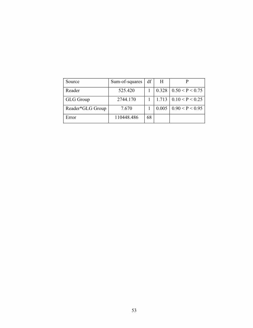
Source Sum-of-squares df H P
Reader 525.420 1 0.328 0.50 < P < 0.75
GLG Group 2744.170 1 1.713 0.10 < P < 0.25
Reader*GLG Group 7.670 1 0.005 0.90 < P < 0.95
Error 110448.486 68
53

54
Figure 5. Age-bias plots for two different viewing platforms, (a) Reader 1 and (b)
Reader 2. The 1:1 line is included for reference to illustrate how the plot would
look if there were complete concordance in age estimates between readers.

02468
1012141618202224262830
0 2 4 6 8 10 12 14 16 18 20 22 24 26 28 30
GLGs (Microscope)
GLG
s (Im
age
Ana
lyze
r)
(a:Reader 1)
02468
1012141618202224262830
0 2 4 6 8 10 12 14 16 18 20 22 24 26 28 30
GLGs (Microscope)
GLG
s (Im
age
Ana
lyze
r)
(b:Reader 2)
55

56
Table 7. ANOVA summary for differences in GLG counts between platforms by
age class groups: 0-9 and 10+ for Reader 1 and Reader 2.

Reader 1
Source Sum-of-squares df Mean-square F-ratio P
Age Group 3.053 1 3.053 3.277 0.079
Error 31.670 34 0.932
Reader 2
Source Sum-of-Squares df Mean-Square F-ratio P
Age Group 15.232 1 15.232 5.257 0.028
Error 98.516 34 2.898
57
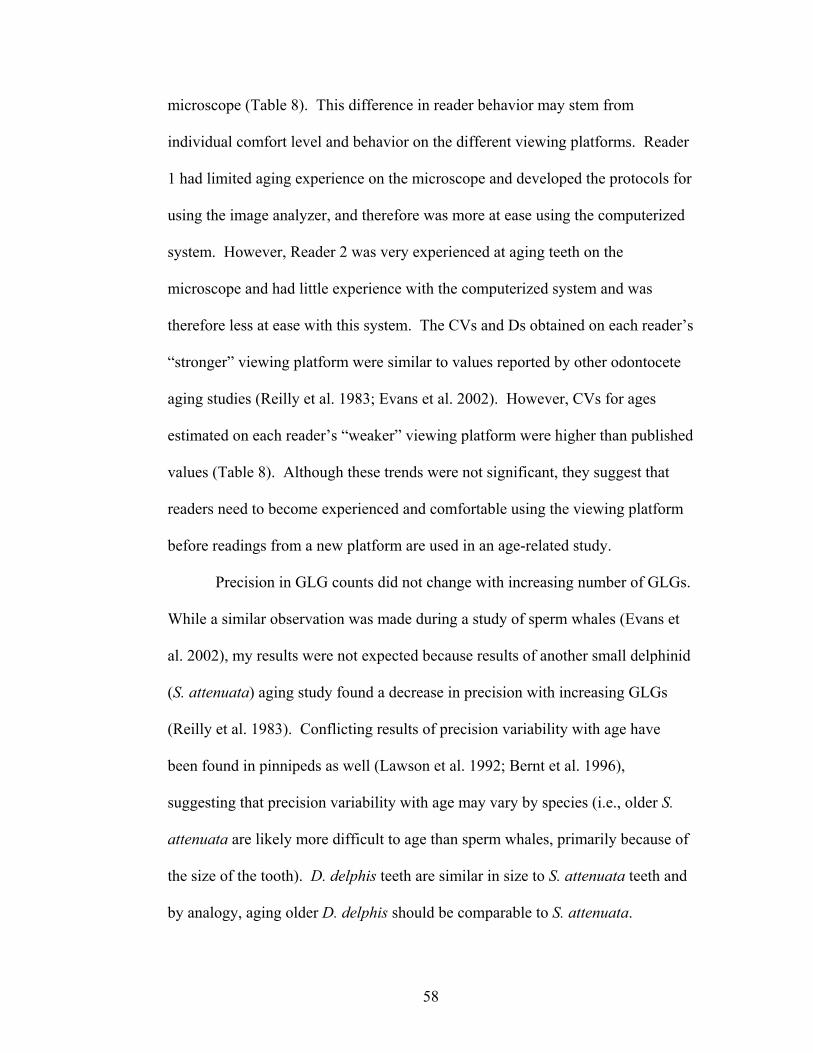
microscope (Table 8). This difference in reader behavior may stem from
individual comfort level and behavior on the different viewing platforms. Reader
1 had limited aging experience on the microscope and developed the protocols for
using the image analyzer, and therefore was more at ease using the computerized
system. However, Reader 2 was very experienced at aging teeth on the
microscope and had little experience with the computerized system and was
therefore less at ease with this system. The CVs and Ds obtained on each reader’s
“stronger” viewing platform were similar to values reported by other odontocete
aging studies (Reilly et al. 1983; Evans et al. 2002). However, CVs for ages
estimated on each reader’s “weaker” viewing platform were higher than published
values (Table 8). Although these trends were not significant, they suggest that
readers need to become experienced and comfortable using the viewing platform
before readings from a new platform are used in an age-related study.
Precision in GLG counts did not change with increasing number of GLGs.
While a similar observation was made during a study of sperm whales (Evans et
al. 2002), my results were not expected because results of another small delphinid
(S. attenuata) aging study found a decrease in precision with increasing GLGs
(Reilly et al. 1983). Conflicting results of precision variability with age have
been found in pinnipeds as well (Lawson et al. 1992; Bernt et al. 1996),
suggesting that precision variability with age may vary by species (i.e., older S.
attenuata are likely more difficult to age than sperm whales, primarily because of
the size of the tooth). D. delphis teeth are similar in size to S. attenuata teeth and
by analogy, aging older D. delphis should be comparable to S. attenuata.
58

59
Table 8. Calculated estimates of precision for individual readers using different
viewing platforms are compared to two other odontocete age studies that
estimated precision.

Reader 1 Reader 2 Reilly et al. Evans et al.
CV D CV D CV D CV D Microscope 11.70 6.75 11.53 6.66 6.90-
11.28 4.55-6.59
10.6 4.8
Image Analyzer 9.00 5.20 14.37 8.30
60

However, the similar precision across age groups found in this study implies that
GLGs in older D. delphis teeth might be less compacted or distorted and thus
have a more consistent layering pattern than other species have. The teeth used in
this study may also have better defined layers due to the temperate habitat they
were collected from. Variation in diet and growth, typical of seasonal habitats,
may lead to more distinct layering in the teeth (Klevezal 1980).
The high CVs for the total pooled mean age estimates on both viewing
platforms were similar to that reported by Reilly et al. (1983) and are likely due to
reader differences in interpretation of the layering patterns of later GLGs. Future
work with older known-age specimens to determine the correct interpretation of
layering patterns could ameliorate large pooled mean CVs by reducing the large
contribution from inter-reader differences. Unfortunately, the availability of older
captive D. delphis teeth is low, and conducting long-term studies of wild
populations are nearly impossible due to the pelagic nature of this species.
Matched paired t-tests and age-bias plots (Figure 4) indicated that GLG
counts were more comparable between readers on the microscope than on the
image analyzer. However, a slight negative bias in Reader 2 GLG counts
(relative to Reader 1) for specimens between four and nine GLGs is apparent on
both viewing platforms. Using image analyzer files, GLG demarcations between
readers were compared on younger specimens to provide insight into potential
reasons for this trend. One explanation may be that Reader 1 counted accessory
lines as growth layers (thus estimating more GLGs) in the younger animals
61

because they are more pronounced in the characteristically wider GLGs typical of
younger ages.
Tooth image files were also examined for specimens contributing to the
positive age-bias of Reader 2 compared to Reader 1 (Figure 4) on both viewing
platforms. A total of three teeth were responsible for the positive bias on the
image analyzer. Pearling, unusual shapes, or shredded areas of the pulp cavity
were present in these teeth, which may have made it more difficult for the less
experienced person (Reader 1) to interpret these inner GLGs, leading to an
underestimation of age (Figure 6). Four teeth in addition to those mentioned
above contributed to Reader 2’s positive bias of middle-aged animals on the
microscope. In these teeth, it is likely that what Reader 1 considered accessory
lines (and therefore did not count), Reader 2 considered GLGs. Reader 2 often
used layers in the cementum to help verify GLG counts in the dentine, whereas
Reader 1 did not. However, Reader 2 could not use this verification method on
the image analyzer because high magnification images of cementum were not
taken. This is likely why the image analyzer does not have as many specimens
contributing to the positive bias in middle aged animals.
The marked negative bias of Reader 2 GLG counts of older animals on the
image analyzer (Figure 4b) stems from differences in reader behavior between
platforms. Age-bias plots (Figure 5) illustrate that Reader 1 had a slight positive
bias for older animals on the image analyzer compared to the microscope and
Reader 2 counted fewer GLGs in older animals on the image analyzer. These
62

63
Figure 6. GLG demarcations of Reader 1 (left) and Reader 2 (right) for specimen
JYB0021. Note increased number of GLGs towards pulp cavity (center) by
Reader 2.

64
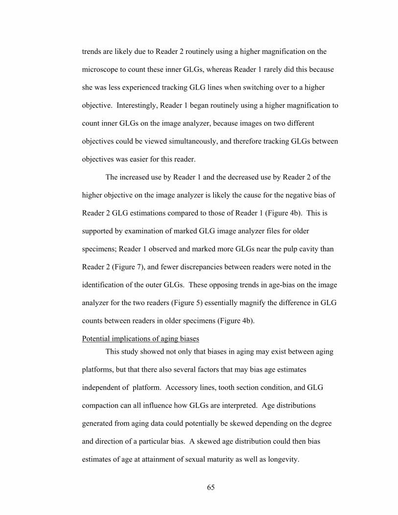
trends are likely due to Reader 2 routinely using a higher magnification on the
microscope to count these inner GLGs, whereas Reader 1 rarely did this because
she was less experienced tracking GLG lines when switching over to a higher
objective. Interestingly, Reader 1 began routinely using a higher magnification to
count inner GLGs on the image analyzer, because images on two different
objectives could be viewed simultaneously, and therefore tracking GLGs between
objectives was easier for this reader.
The increased use by Reader 1 and the decreased use by Reader 2 of the
higher objective on the image analyzer is likely the cause for the negative bias of
Reader 2 GLG estimations compared to those of Reader 1 (Figure 4b). This is
supported by examination of marked GLG image analyzer files for older
specimens; Reader 1 observed and marked more GLGs near the pulp cavity than
Reader 2 (Figure 7), and fewer discrepancies between readers were noted in the
identification of the outer GLGs. These opposing trends in age-bias on the image
analyzer for the two readers (Figure 5) essentially magnify the difference in GLG
counts between readers in older specimens (Figure 4b).
Potential implications of aging biases
This study showed not only that biases in aging may exist between aging
platforms, but that there also several factors that may bias age estimates
independent of platform. Accessory lines, tooth section condition, and GLG
compaction can all influence how GLGs are interpreted. Age distributions
generated from aging data could potentially be skewed depending on the degree
and direction of a particular bias. A skewed age distribution could then bias
estimates of age at attainment of sexual maturity as well as longevity.
65

66
Figure 7. GLG demarcations of specimen SHB003 by Reader 1 (left side with
lower inset of higher magnification) and Reader 2 (right side). Note greater
number of GLGs towards pulp cavity (center) for Reader 1.

67
67

Unfortunately, the degree and direction of a bias from “true” age is not often
known.
Conclusions
Comparable precision to traditional light microscopy, ability to reference
GLG demarcations to resolve reader differences in age, and use as a storage
medium resistant to fading make digital microscope images in combination with
image analysis software a promising tool for GLG estimation in small delphinid
teeth. However, before this system can be used as a standard procedure for age
related studies, additional analyses similar to this need to be performed after
readers have gained sufficient experience with the system and a standard protocol
is in place for using higher objectives and cementum layers to aid in GLG
estimation of older animals. If GLG counts in the cementum are needed to verify
GLG counts in the dentine, high magnification images of the cementum should be
taken. If reader behavior were comparable after such protocols were implemented
and experience was gained, image analysis would be the preferred method for
aging delphinid teeth.
68

CHAPTER 4: GROWTH AND REPRODUCTION OF FEMALES
Introduction
In the ETP, research on D. delphis has been limited to stock structure,
reproductive rates, and timing of reproduction (Henderson et al. 1980; Perryman
and Lynn 1993; Dizon et al. 1994). Using data from 1973 to 1978, Henderson et
al. (1980) summarized reproductive phase lengths and pregnancy rates for
females of the central stock, whose boundaries differed slightly from those
currently used and described in Perrin et al. (1985). Using current stock
boundaries, Perryman and Lynn (1993) described patterns in timing of
reproduction for all three stocks, using aerial photogrammetry.
However, the literature is incomplete and does not contain any estimates
of length at birth, average age and length at attainment of sexual maturity,
individual growth rates, senescence, and longevity of D. delphis in the ETP. The
purpose of this paper is to describe the life history of females from the central
stock of D. delphis in the ETP. In addition to presenting estimates of growth and
reproductive parameters, I compare the life history parameters to those described
for the species in the North Pacific (Ferrero and Walker 1994) and to other small,
pelagic dolphins (S. attenuata and S. longirostris) inhabiting the ETP.
Methods
Specimen and Data Collection
Scientific observers from the NMFS and the Inter-American Tropical
Tuna Commission (IATTC) collected field and biological data from dolphins
69

incidentally killed in the tuna purse seine fishery. Specimens were processed
using the methods of Perrin et al. (1976a). Total body length of animals was
measured to the nearest centimeter. Mammaries were examined for the presence
of milk, reproductive tracts were collected and preserved in 10% formalin, and
teeth were collected from the left lower jaw at midlength. Biological data and
tissue samples were only collected from a subset of the observed kill.
In the laboratory, ovaries were weighed and examined for the presence of
corpora lutea and/or corpora albicantia. If present, these were then counted and
classified as described by Akin et al. (1993). Total corpus count was defined as
the number of corpora albicantia and corpora lutea present on both the left and
right ovaries. Females were considered to be sexually mature if their total corpus
count was greater than zero. The reproductive tract was inspected carefully for
the presence of a fetus, especially if a corpus luteum was present. Fetuses were
sexed, weighed and measured (Akin et al. 1993).
Total body length, collection date, and collection location were recorded
for 1,330 female D. delphis collected between 1973 and 1993 (Figure 8). Age
and reproductive status were determined for 506 and 880 of these specimens,
respectively.
Tooth Preparation and Examination
Following the protocol of Myrick et al. (1983), teeth were decalcified, cut
with a freezing microtome into 25 µm-thick longitudinal serial sections, and
stained with hematoxylin. Sections were mounted on gelatin-coated slides, and
cover slip margins were sealed with DPX mounting medium (Lockyer 1995).
70

71
Figure 8. Collection locations of 1330 central stock female D. delphis sampled.
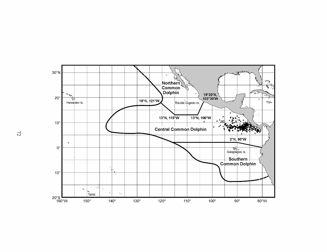
72

Ages were determined by GLGs in the dentine (Myrick et al. 1983; Hohn et al.
1989) under a compound light microscope at 40x and 100x magnification. Each
GLG is interpreted as representing one year of life on the basis of the calibration
study by Gurevich et al. (1980).
Two readers aged each tooth three times, with at least a week between
readings. GLG counts were made without reference to specimen information,
such as total body length, reproductive status, or previous GLG counts. The mean
GLG count of both readers’ three readings is referred to as the total pooled mean
age estimate, whereas the mean for an individual reader is referred to simply as
mean age estimate. Pooled mean age estimates were used in all analyses of
reproduction and individual growth data. Coefficient of variation (CV =
100×Χ
SD ) was used to measure the precision of age estimates (Chang 1982).
Stable Age Distribution
A predicted stable age distribution was generated using the proportion of
animals expected in each age class based on a leslie matrix model using spinner
dolphin age-specific survival rates (Chivers 2002b).
Length and Age Parameter Estimation
Three methods were used for estimating length at birth and age and length
at attainment of sexual maturity: (a) the sum-of-fraction-immature method (Hohn
1989), (b) the DeMaster (1978) method, and (c) logistic regression. These
methods were used as a means to compare parameters to other studies and to
determine the best estimator for this study.
73

Sum-of-fraction immature method
The sum-of-fraction immature (SOFI) method estimates the average age at
attainment of sexual maturity (ASM) as
ASM = j + , ∑=
k
jiii xp (1)
where j is the age of the youngest mature animal, k is the age of the oldest
immature animal, pi is the proportion of immature animals in age class i, and xi is
the number of age classes combined in age class i. Variance was estimated as
var (ASM) = ∑ , = −
−k
ji i
iii
nxpp
1)1( (2)
where ni is the sample size for age class i.
To estimate average length at attainment of sexual maturity (LSM), the
SOFI method was modified to use constant length intervals (5 cm) instead of ages
so that
LSM = j + , ∑=
max
min
i
iiii xp (3)
where j is the lower limit of the length class with the smallest mature animal, imin
is the length class with the shortest mature animal, imax is the length class with the
longest immature animal, pi is the proportion of immature animals in length class
i, and xi is the number of age classes combined in age class i. Variance was
estimated as
var (LSM) = ∑= −
−max
min1
)1(i
ii i
iii
nxpp , (4)
where ni is the total number of animals in the ith length class.
74
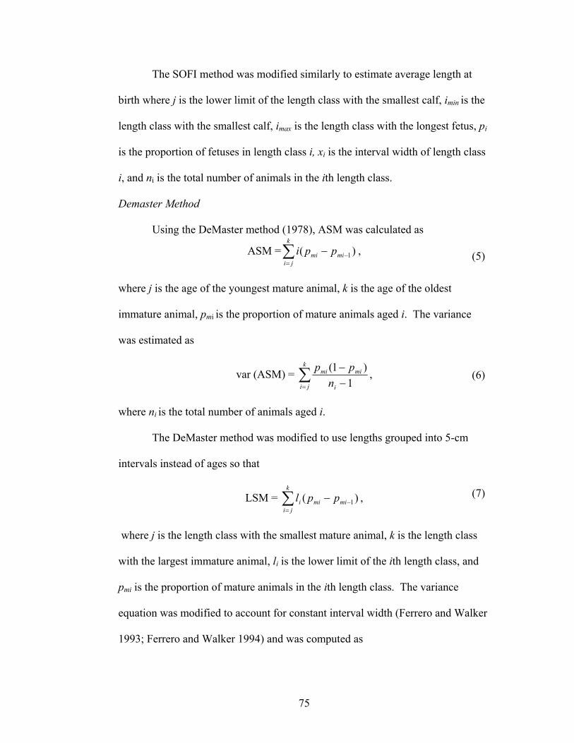
The SOFI method was modified similarly to estimate average length at
birth where j is the lower limit of the length class with the smallest calf, imin is the
length class with the smallest calf, imax is the length class with the longest fetus, pi
is the proportion of fetuses in length class i, xi is the interval width of length class
i, and ni is the total number of animals in the ith length class.
Demaster Method
Using the DeMaster method (1978), ASM was calculated as
ASM = , )( 1∑=
−−k
jimimi ppi (5)
where j is the age of the youngest mature animal, k is the age of the oldest
immature animal, pmi is the proportion of mature animals aged i. The variance
was estimated as
var (ASM) = ∑= −
−k
ji i
mimi
npp1
)1( , (6)
where ni is the total number of animals aged i.
The DeMaster method was modified to use lengths grouped into 5-cm
intervals instead of ages so that
LSM = , ∑=
−−k
jimimii ppl )( 1
(7)
where j is the length class with the smallest mature animal, k is the length class
with the largest immature animal, li is the lower limit of the ith length class, and
pmi is the proportion of mature animals in the ith length class. The variance
equation was modified to account for constant interval width (Ferrero and Walker
1993; Ferrero and Walker 1994) and was computed as
75

var (LSM) = w2 ∑= −
−k
ji i
mimi
npp1
)1( (8)
where w is the constant interval width and ni is the number of animals in the ith
length class.
Since negative values of pmi were present in the length and age datasets,
new predicted proportions were calculated from a nonlinear curve fitted to a plot
of proportion mature versus age and length (Laws et al. 1975) and entered into the
models.
Logistic Regression
Logistic regression analysis, based on maximum likelihood, was used to
estimate ASM and LSM by determining the length and age at which 50% of a
combined sample of immature and mature animals was predicted to be mature.
Similarly, logistic regression was used to determine estimated length at birth
(ELB) by determining the length at which 50% of a combined sample of fetuses
and post-natal specimens was predicted to be born. To increase sample size, both
males and females were used to estimate length at birth. Confidence intervals
were constructed based on 1,000 bootstrap replicates conducted by sampling the
data with replacement.
To determine whether the calculated mean length at birth is significantly
biased by undocumented calf mortality (i.e., missing calves in the data set; Archer
et al. 2001), an alternative estimate of length at birth was calculated (using the
logistic regression method) based on a hypothetical data set and then compared to
the original estimate. The hypothetical data set added 15% more (+8) calves,
76
which is the upper range of undocumented mortality estimated by Archer et
al.(2001), to the smallest indeterminate length class (75 cm).
To test the null hypothesis that the original ELB and the hypothetical ELB
were the same, the data sets were permuted, and a P-value calculated for the
comparison. The permuted data sets were created by pooling the original and
hypothetical data sets, then creating 1000 new data sets of two groups (with
original n) through random sampling of the pooled group. The P-value is the
proportion of the runs that the difference in ELB between the permuted data sets
was greater than or equal to the observed difference between the original and
hypothetical data set.
Comparison of methods
For this study, the preferred method for calculating ASM, LSM and ELB
is the logistic regression followed by the SOFI method. The DeMaster method
was least favorable because of the need to calculate new predicted proportions
that the variance calculation does not take into account. The advantage of the
SOFI and logistic methods was that they could be used with the original raw data
set. However, the binning required for the SOFI method likely results in a loss of
resolution, and the associated variance appears to be underestimated. The ability
to input raw data and to capture the variance of the fit with bootstrap replicate
sampling makes the logistic regression method preferable and it is thus used in all
parameter comparisons in this study.
Age at conception and first birth
Age at conception was calculated by subtracting the age of the fetus
(estimated from fetal length; see Table 9) from the age of the female on the day of
77
78
Table 9. Age of conception was calculated for pregnant females with one corpus
luteum and no corpora albicantia. Fetus age was based on fetal growth model
developed by S. Chivers.

SPECIMEN
Age on day of collection
(years)
Age of conception (mother's age - fetus age)
(years)
Fetus Length (cm)
Fetus Age
(days)
Fetus Age
(years)JEJ0021 9.2 9.2 0.1 2 0.006 TBS0216 10.8 10.8 0.5 5 0.014 MAK0241 9.2 9.0 16 79 0.216 PLR0022 8.0 7.8 16.3 80 0.219 JHT0074 9.5 9.2 19.5 92 0.252 RWC0469 6.8 6.3 49 202 0.553 REB0033 10.8 10.0 78 317 0.869 RJO0384 8.3 7.5 78.2 318 0.871 WCF0105 14.0 13.1 80 325 0.890 WCF0098 9.8 8.9 85 344 0.943
79

collection. This calculation was based on pregnant females with one corpus
luteum and no corpora albicantia and excluded one 16-year-old, considered to be
an outlier in the data set. Mean age at first birth was estimated using only the
lactating females with one corpus.
Gestation
Gestation was estimated using Perrin et al.’s (1977) regression equation,
Log (y) = 0.1659 + 0.4856 Log (x), (9)
where y is the length of gestation and x is the length at birth. This equation is
based on the positive correlation between length at birth and gestation of four
closely related delphinids.
Growth
Using the Laird-Gompertz formula (Laird 1969), a two-phase growth
model (Perrin et al. 1976a; Perrin et al. 1977) was used to simultaneously fit
separate equations to female age at length data, using an iterative least-squares
method. The Laird-Gompertz model is
))) (1(()(tea
o eLtLα−−∗= (10)
where L(t) is length at time t, Lo is the length at birth, t is the age, a is the specific
rate of exponential growth, and α is the rate of decay of exponential growth. The
first model was anchored at the ELB. The intersection point of the two models
was estimated as the age at which the total sum of squares for the fit of both
models was smallest.
Seasonality
Birth dates for animals estimated to be less than one year old (i.e., total
length ≤ 134 cm) were back-calculated using,
80
db = dc – 30 r
ll bc − (11)
where db is the day of the year of the birth date, dc is the day of the year of
collection, lc is the length at collection, lb is length at birth, and r is growth rate
in centimeters per month. The ELB derived from the logistic method was
rounded down and used as an estimate of lb. The growth rate of 4.1 cm/month
obtained from the previously described growth model was used as the estimate for
r.
Reproductive Phases and Calving Interval
The proportion of pregnant, lactating, and resting (those neither pregnant
or lactating) females (Table 10) was used in combination with the gestation period
to determine estimates of the calving interval (Perrin et al. 1976a). The
summation method (gestation + lactation + resting phases) and the reciprocal of
the APR were used to calculate two estimates of calving interval (Perrin et al.
1976a). Both of these methods are based on the likely invalid assumption of no
fetal mortality (Perrin et al. 2003). The equations for estimating time spent
lactating and resting, and APR are:
Lactation = GPL× (12)
Resting = GPR× (13)
APR= GP (14)
where, L is the proportion of sexually mature females lactating (including those
simultaneously pregnant), P is the proportion of sexually mature females pregnant
81

82
Table 10. Reproductive condition of 440 sexually mature female D. delphis
collected between 1973 and 1993.
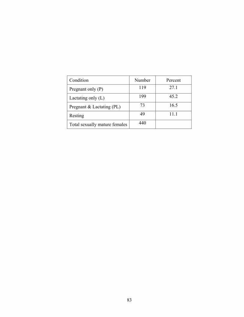
Condition Number Percent
Pregnant only (P) 119 27.1
Lactating only (L) 199 45.2
Pregnant & Lactating (PL) 73 16.5
Resting 49 11.1
Total sexually mature females 440
83

(including those simultaneously lactating), G is the length of gestation in years,
and R is the proportion of sexually mature females neither pregnant nor lactating.
Results
The Sample
To assess potential subsampling biases of the aged and reproductive
samples, the length frequency distributions of these subsamples were compared to
that of the total sample. The median length value of these subsamples (191 cm
and 189 cm) were within the median 95% confidence interval (143 - 202.5 cm) of
a bootstrap replicate sample of 1000 (based on the total sample), indicating that
these were random subsamples of the entire sample. Lengths and ages of female
D. delphis ranged from 84 to 213 cm (Figure 9) and 0 to 25 years (Figure 10),
respectively. The age distribution is bimodal (Figure 10), with peaks in the age
classes of juveniles (i.e., three and four year olds) and sexually mature adults (i.e.,
11 to 13 year olds). This is quite different from what is expected under a stable
age distribution (Figure 10). For delphinids, the greatest frequency of animals is
expected to be neonates, followed by yearlings, juveniles, and adults (Figure 10).
Aging
The calculated CVs for Reader 1, Reader 2, and the pooled mean age
estimate were 17.3%, 14.0%, and 21.0%, respectively. A Spearman rank
correlation test for each reader indicates that there is no relationship between CV
and mean age estimate (Reader 1, P = 0.610; Reader 2, P = 0.658). Between
readers, 58 % of readings agreed to within one year and 76% agreed to within two
years. Mean age estimates were not significantly different between readers
84

85
Figure 9. Total body length frequency distribution of central female D. delphis
sampled (n = 1330). The x-axis labels represent the upper bound of the length
interval.

050
100150200250300350400450
70 80 90 100
110
120
130
140
150
160
170
180
190
200
210
220
Length
Freq
uenc
y
86

87
Figure 10. Age frequency distribution of sampled central female D. delphis (gray
bars only; n = 506) and predicted stable age distribution (gray + black bars)
typical for small delphinids.

0
20
40
60
80
100
120
140
0 1 2 3 4 5 6 7 8 9 10 11 12 13 14 15 16 17 18 19 20 21 22 23 24 25
Age (years)
Num
ber o
f ind
ivid
uals
88

(Wilcoxin Signed-Rank Test: z = 0.627, P = 0.531). However, a plot of age
differences between readers illustrates that compared to Reader 1, Reader 2
tended to estimate higher for younger animals and lower for older animals (Figure
11).
Length at Birth
The smallest calf was 75 cm long and the largest fetus was 88 cm. The
mean length of the 19 fetuses and 9 calves within that length range (Figure 12) is
82.7 cm (n = 28; 17 male, 11 female, SE = 0.732).
Using logistic regression (Figure 13) and a modified SOFI method based
on 5-cm groupings, ELBs are 85.2 cm (95% CI, 82.9-87.1) and 85.5 cm (SE =
0.092), respectively. All female postnatal specimens, male postnatal specimens ≤
98 cm, and fetuses (regardless of gender) with an associated total body length
were used in the logistic regression analysis.
Gestation
Using the ELB of 85.2 cm, gestation was estimated to be 11.3 months.
This estimate could not be compared to the method of Hugget and Widdas (1951)
because the available data violated the assumption that reproduction is seasonal.
The linear phase of fetal growth required for this method could not be estimated
using this data set, because fetuses of all lengths and therefore ages were present
throughout the year (Figure 14).
Postnatal Growth
Growth was rapid through age 2 with predicted lengths of one- and two-
year olds of 133.9 cm and 159.3 cm, respectively (Figure 15). After age two,
89

90
Figure 11. Differences in mean age estimates (years) between readers across
ages. Compared to Reader 1, a positive bias in younger animals and a negative
bias in older animals are present for Reader 2.

-15
-10
-5
0
5
10
15
0 5 10 15 20 25 30 35
Age estimated by reader 1 (years)
Diff
eren
ce b
etw
een
read
er 1
and
read
er 2
91

92
Figure 12. Length frequency distribution for 19 fetuses and 9 calves (males and
females) of central D. delphis within the overlapping length range of smallest calf
and largest fetus.

93
0
2
4
6
8
10
12
75-79 80-84 85-89
Length (cm)
Freq
uenc
y
fetuscalves

94
Figure 13. A logistic curve fitted to length and postnatal status. The length at
which 50% of specimens are predicted to be calves equals 85.2 cm (95% CI, 82.9
- 87.1 cm), the estimated length at birth. The circles represent individual samples.
Range of x-axis limited for presentation.

95
0
0.1
0.2
0.3
0.4
0.5
0.6
0.7
0.8
0.9
1
60 70 80 90 100
Length (cm)
% P
ostn
atal
85.2 cm

96
Figure 14. Scatterplot of fetal lengths and day of collection.

97
R2 = 0.0008
0
10
20
30
40
50
60
70
80
90
100
0 30 60 90 120 150 180 210 240 270 300 330 360
Collection Day of Year
Fetu
s Len
gth
(cm
)

98
Figure 15. Two-phase Laird-Gompertz growth model fit to female D. delphis age
at length data. The predicted asymptotic length from the model was 196.5 cm.

8090
100110120130140150160170180190200210220
0 5 10 15 20 25 30
Age (years)
MatureImmature
196.5Le
ngth
(cm
)
99

growth slowed until 5.48 years, where growth rate increased again. Growth
subsequently slowed again until it reached an asymptote of 196.5 cm.
Sexual Maturation
The youngest sexually mature female was 5 years old and the oldest
sexually immature female was 14 years old (Figure 16a). The average ASM was
estimated to be 8.0 years (SE = 0.013) using the SOFI Method, 8.1 years (95%
CI, 7.7 - 8.5) using the Logistic Method (Figure 17), and 8.0 years (SE = 0.013),
using the DeMaster (1978) method. The mean age of first conception was
estimated to be 8.7 years (n = 10, SE = 0.601). On average, females gave birth
for the first time at 10 years of age (n = 10, SE = 0.791).
Length and Sexual Maturation
Sexually mature females ranged in length from 172 to 213 cm (Figure
16b) and averaged 195.2 cm in length (n = 461, SE = 0.317). The largest sexually
immature female was 205 cm long (Figure 16b). Using the modified SOFI
method, modified DeMaster, and logistic methods (Figure 18), length at sexual
maturity was estimated to be 186.4 cm (SE = 0.008), 184.4 cm (SE = 0.018), and
185.9 cm (95% CI, 185.0-186.7), respectively.
Ovulation
Total corpus counts in sexually mature females ranged from 1 to 30. A
regression of mean number of corpus scars on age class shows a significant
increase in corpus scars with age (P < 0.001) (Figure 19). To fit this regression,
corpus counts for the youngest and oldest ages were combined so that sample
sizes were greater than five for the 5 and 20 year age classes. Among mature
100

101
Figure 16. Scatterplot of total corpora count of central female D. delphis as a
function of (a) age (n = 506) and (b) length (n = 880).
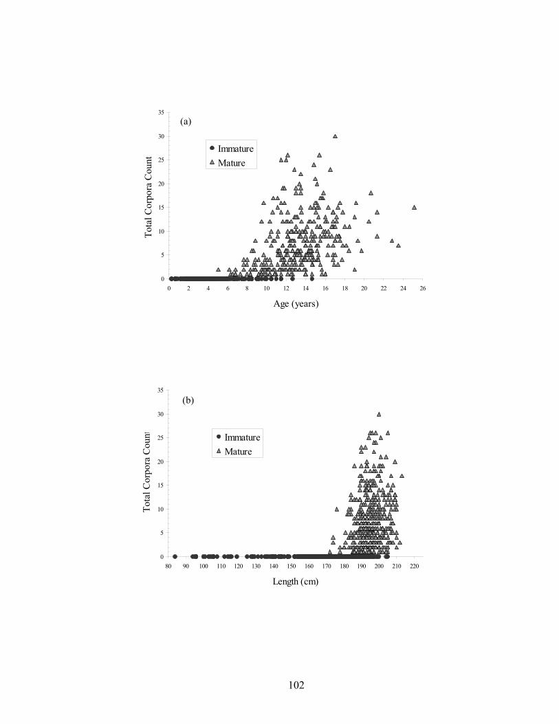
102
0
5
10
15
20
25
30
35
80 90 100 110 120 130 140 150 160 170 180 190 200 210 220
Length (cm)
Tota
l Cor
pora
Cou
nt ImmatureMature
(b)
0
5
10
15
20
25
30
35
0 2 4 6 8 10 12 14 16 18 20 22 24 26
Age (years)
Tota
l Cor
pora
Cou
ntImmatureMature
(a)

103
Figure 17. A logistic curve fitted to age and maturity status. The length at which
50% of specimens are predicted to be mature equals 8.1 years (95% CI, 7.6 - 8.5
years), the estimated ASM. The circles represent individual samples.

104
0
0.1
0.2
0.3
0.4
0.5
0.6
0.7
0.8
0.9
1
0 2 4 6 8 10 12 14 16 18 20 22 24 26 28
Age (years)
8.1
% m
atur
e

105
Figure 18. A logistic curve fitted to length and maturity status. The length at
which 50% of specimens are predicted to be mature equals 185.9 cm (95% CI,
184.9 - 186.8 cm), the estimated LSM. The circles represent individual samples.

106
0
0.1
0.2
0.3
0.4
0.5
0.6
0.7
0.8
0.9
1
80 100 120 140 160 180 200 220
Length (cm)
185.9
% m
atur
e
107
Figure 19. Mean number of corpora scars increases with age in central D. delphis
(P < 0.001). Points represent means for one-year age classes. Vertical bars
represent standard errors of the mean count for each age class.

y = 0.6983x - 1.6809R2 = 0.8753
0
2
4
6
8
10
12
14
16
0 5 10 15 20 25
Age (years)
Mea
n nu
mbe
r of c
orpo
ra sc
ars
108

females, the mean number of corpus scars was greater in the left ovary than in the
right ovary (Wilcoxin Rank Sum Test: z = -22.464, P = 0.0000). In fact, at least
90% of the first three ovulations occur in the left ovary. A gradual shift to using
both ovaries occurs with increasing corpora. After 15 corpora have accumulated
this shift becomes more pronounced (Table 11).
Seasonality
No clear peaks in birth dates were indicated in the resulting distribution of
back-calculated birth dates (Figure 20). The Kuiper’s test demonstrates that birth
dates were not significantly different (K = 1.0, P > 0.10) from a uniform
distribution (Figure 20), indicating no seasonality in female reproduction.
Reproductive Phases and Calving Interval
The summation of the gestation (11.3 months), lactation (16.1 months),
and resting (2.9 months) phases estimated a calving interval of 30.3 months, or
2.5 years. The second estimate of 25.9 months, or 2.15 years was derived from
the reciprocal of the APR (1/0.466). This estimate of the calving interval is likely
lower than that calculated from the sum of reproductive phases, because it
includes 26.8 % of lactating females that are simultaneously pregnant, whereas
the other calving interval estimate is the sum of the observed reproductive phases
of females whose reproductive phases do not overlap. Additionally, the data set
shows that pregnancy and lactation rates change with age. That is, pregnancy rate
decreases with increasing age as lactation rates increase (Figure 21).
109

110
Table 11. Location of corpora (corpora lutea and corpora albicantia) in the
ovaries of 460 central D. delphis.
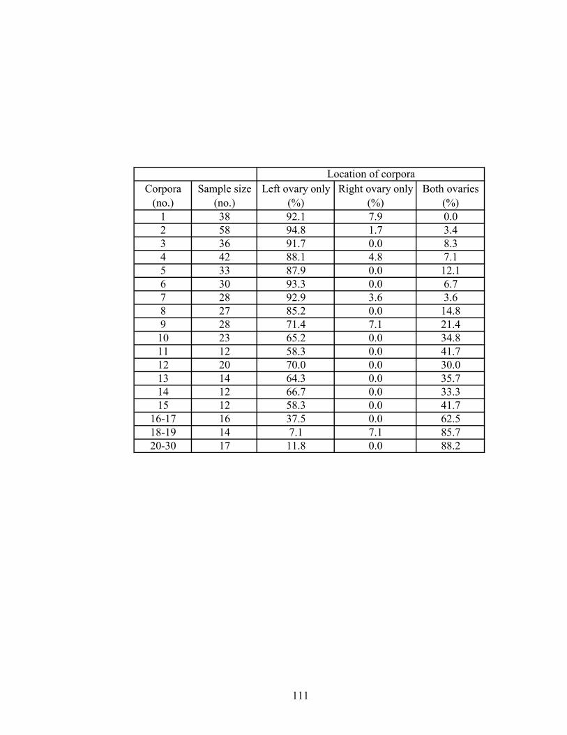
111
Corpora (no.)
Sample size (no.)
Left ovary only (%)
Right ovary only (%)
Both ovaries (%)
1 38 92.1 7.9 0.02 58 94.8 1.7 3.43 36 91.7 0.0 8.34 42 88.1 4.8 7.15 33 87.9 0.0 12.16 30 93.3 0.0 6.77 28 92.9 3.6 3.68 27 85.2 0.0 14.89 28 71.4 7.1 21.410 23 65.2 0.0 34.811 12 58.3 0.0 41.712 20 70.0 0.0 30.013 14 64.3 0.0 35.714 12 66.7 0.0 33.315 12 58.3 0.0 41.7
16-17 16 37.5 0.0 62.518-19 14 7.1 7.1 85.720-30 17 11.8 0.0 88.2
Location of corpora

112
Figure 20. Distribution of cumulative back-projected birth-dates. The observed
cumulative distribution is not significantly different from an expected uniform
cumulative distribution (P > 0.10), indicating no seasonality in female
reproduction. Bars indicate frequency of back-calculated birth-dates of female (n
= 66) and male (n = 68) D. delphis ≤ 134 cm.

113
0.0
0.2
0.4
0.6
0.8
1.0JA
N
FEB
MA
R
APR
MA
Y
JUN
JUL
AU
G
SEP
OC
T
NO
V
DEC
Month
0
2
4
6
8
10
12
14
16
18
Freq
uenc
y
ObservedExpected
Cum
ulat
ive
Prop
ortio
n

114
Figure 21. Plot of proportion of females pregnant and proportion lactating on age.
The proportion of pregnant females decreases with age, along with a concomitant
increase of proportion lactating. Dashed lines represent how data were binned to
calculate proportions, with samples sizes in parentheses.

0
0.1
0.2
0.3
0.4
0.5
0.6
0.7
0.8
0 5 10 15 20 25
Age
Prop
ortio
n of
sexu
ally
mat
ure
fem
ales
pr
egna
nt o
r lac
tatin
g
pregnantlactating
(42) (194) (83)
115

Post-Reproductive Females
Following the criteria of Perrin et al. (1977), 440 sexually mature females
were examined for evidence of senescence. The five criteria indicative of
senescence are: (1) neither pregnant or lactating, (2) ≥ 10 corpora, (3) ovaries
weigh < 3.5 g, (4) no developing follicles, (5) no Type 1 or 2 corpora albicantia.
None of the 440 animals showed clear evidence of being post-reproductive since
none met all five criteria. Ten specimens met at least three of the five criteria, and
two specimens met four (Table 12).
Discussion
The age distribution of the sample is markedly different from that of
female S. l. orientalis (Chivers 2002b) and more similar to that of female S.
attenuata (Barlow and Hohn 1984) that inhabit the same area and are impacted by
the same fishery. Both calves and juveniles are underrepresented in the age
distributions of D. delphis (Figure 10) and S. attenuata (Barlow and Hohn 1984)
when compared to an expected stable age distribution. Several alternative
explanations for the age distribution in S. attenuata were outlined by Barlow and
Hohn (1984), which include (a) school segregation, (b) a variable rate of tooth
deposition, and (c) non-stable age distribution reflecting large perturbation in the
population.
If schools are segregated by age or reproductive class, juvenile animals
may inhabit different areas, or they may not join herds that associate with tuna
that are targeted by the purse-seine fishery. Kleinenberg (1956) and Tomlin
(1957) documented herd segregation of D. delphis in the Black Sea, where
116

117
Table 12. D. delphis specimens that possess at least three of five criteria elements
indicative of senescence.

Specimen No. Total Corpora Resting Ovaries<3.5 g No developing follicles No type 1 or 2 corpora DAM0039 26 X X X MAJ0014 25 X X XWOK0056 13 X X JJN0063 19 X X REL0160 19 X X JEJ0103 16 X X RDP0120 11 X X AGA0012 26 X X DJG0094 12 X X NWV0132 10 X X
118

females predominantly occur offshore during periods of calving and early
lactation. Population segregation has been suggested for the North Pacific
population of D. delphis (Ferrero and Walker 1994) to explain the paucity of
pregnant females and neonates in their sample collected from a high-seas driftnet
fishery.
Variable tooth rate deposition could lead to misinterpretations of growth
layers leading to inaccurate estimates of ages. Since the age distribution of D.
delphis in the N. Pacific (Figure 22) is quite different from that found in the ETP
(Figure 10), variable tooth rate deposition for this species seems a less likely
hypothesis and may reflect inherent sampling biases of the two fisheries.
However, it is conceivable that tooth rate deposition could vary within a species
in response to habitat or prey differences and therefore could still be a possible
explanation. Exploring this explanation further is complicated because there are
likely other biases or inaccuracies in reading GLGs in the teeth.
Incidental mortality in the purse-seine fishery certainly has served as a
large perturbation in the population with central D. delphis mortality peaking at
21,299 in 1973 during the years of this study (Smith 1979; Bayliff 2002).
However, considering the evidence for segregation in other D. delphis
populations, this may be the more likely explanation for the observed age
distribution than a non-stable age distribution of the population. The “dip” in
animals less than two years may also be a sampling artifact, partially explained by
limited sampling of these age classes by observers and calves that were initially
present in the school but not caught in the purse-seine net (Archer et al. 2001).
119

120
Figure 22. Age distribution of female D. delphis in the N. Pacific. Data taken
from Ferrero and Walker (1994).

02468
10121416
0 2 4 6 8 10 12 14 16 18 20 22 24
Age (years)
Num
ber o
f ind
ivid
uals
121
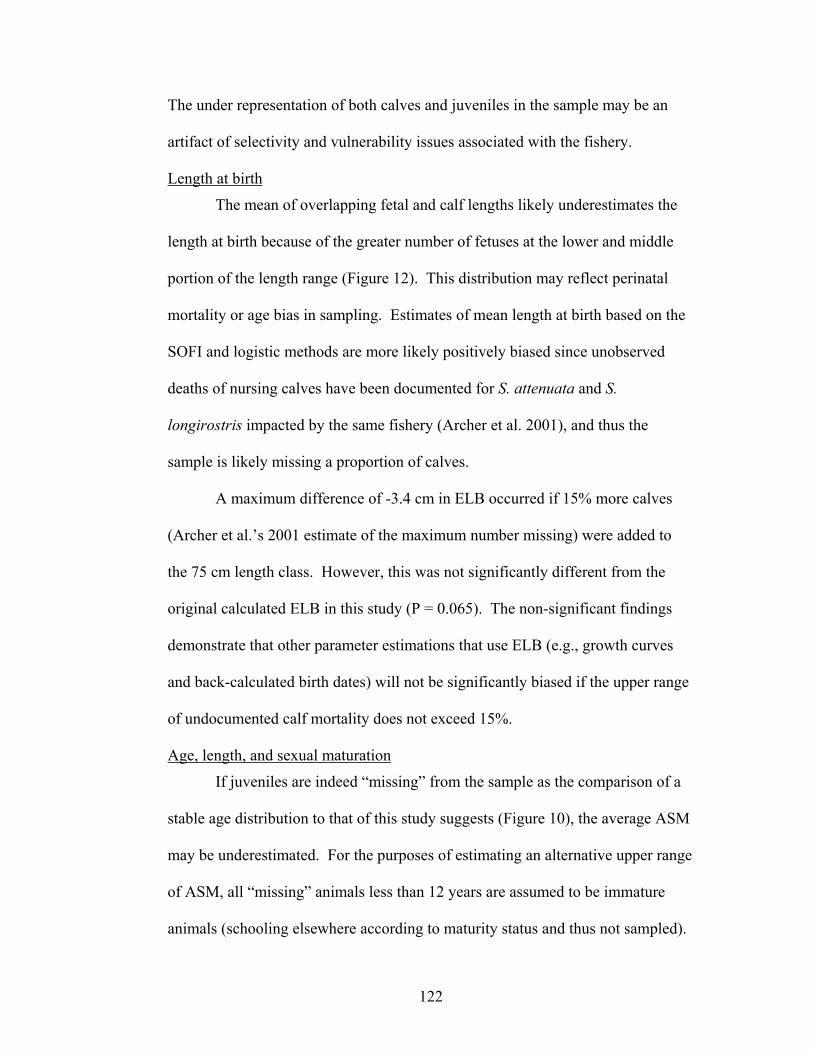
The under representation of both calves and juveniles in the sample may be an
artifact of selectivity and vulnerability issues associated with the fishery.
Length at birth
The mean of overlapping fetal and calf lengths likely underestimates the
length at birth because of the greater number of fetuses at the lower and middle
portion of the length range (Figure 12). This distribution may reflect perinatal
mortality or age bias in sampling. Estimates of mean length at birth based on the
SOFI and logistic methods are more likely positively biased since unobserved
deaths of nursing calves have been documented for S. attenuata and S.
longirostris impacted by the same fishery (Archer et al. 2001), and thus the
sample is likely missing a proportion of calves.
A maximum difference of -3.4 cm in ELB occurred if 15% more calves
(Archer et al.’s 2001 estimate of the maximum number missing) were added to
the 75 cm length class. However, this was not significantly different from the
original calculated ELB in this study (P = 0.065). The non-significant findings
demonstrate that other parameter estimations that use ELB (e.g., growth curves
and back-calculated birth dates) will not be significantly biased if the upper range
of undocumented calf mortality does not exceed 15%.
Age, length, and sexual maturation
If juveniles are indeed “missing” from the sample as the comparison of a
stable age distribution to that of this study suggests (Figure 10), the average ASM
may be underestimated. For the purposes of estimating an alternative upper range
of ASM, all “missing” animals less than 12 years are assumed to be immature
animals (schooling elsewhere according to maturity status and thus not sampled).
122

If “missing” animals from the stable age distribution (Figure 10) were included in
the logistic regression analysis, ASM was calculated as 10.2 years. (95% CI, 9.9 -
10.4), which is two years older than I calculated using the data available. This
alternative estimate of ASM must be considered in population models of female
central D. delphis.
A difference exists between the average ASM and mean age at first
conception (0.7 years or 8.4 months), indicating that females do not conceive
immediately following attainment of sexual maturity. Alternatively, it could be a
result of the potential negative bias in the average ASM. In addition, the time
between mean age of conception and mean age at first birth exceeds the gestation
period by 4.3 months. This may indicate that perhaps some females may abort
after first conception and become pregnant again, thus extending the time from
first conception and first birth past the expected gestation time. These differences
may exist because fertility and reproductive success are generally depressed in
newly mature female cetaceans (Boyd et al. 1999).
The mean length of sexually mature females (195.2 cm) is comparable to
previous mean adult length estimates of 194.3 cm (Perrin et al. 1985) and 194.8
cm (Perryman and Lynn 1993) for central D. delphis females.
Ovulation
The wide scatter in the plot of corpora on age for all individuals (Figure
16a) demonstrates the individual variation in ovulation rates that has also been
documented in studies of other species (Perrin et al. 1976b; Perrin et al. 1977;
Myrick et al. 1986). Individuals do not necessarily begin to ovulate at the same
age and thus the slope of the regression of number of corpora on age class should
123
not be used as the average ovulation rate. The asymmetry of corpora scars in
each ovary indicates that there is a prevalence of activity in the left ovary, similar
to what has been found in other delphinids (Perrin et al. 1976a; Perrin et al. 1977).
Reproductive phases and calving interval
The observation that pregnancy rate decreases and lactation period
increases with age (Figure 21) suggests that either younger females wean their
calves earlier or do not successfully rear their calves, thus becoming pregnant
more often than older females.
Lactation and resting phases and both estimates of calving interval are
based on the assumption of no fetal mortality and are therefore minimum
estimates. If central D. delphis experiences high fetal mortality rates similar to
other ETP dolphins (Perrin et al. 2003), the observed proportion of pregnant
females would be inflated by animals experiencing multiple re-impregnations
following miscarriages. If fetal mortality were significant, calculated
reproductive phases and calving intervals would be underestimates and APR
overestimated because they are based simply on the proportion of pregnant
females in the sample. Perrin et al. (2003) incorporated fetal mortality estimates
to adjust the average calving interval of S. attenuata and S. longirostris from 3 to
5 years, and if true for D. delphis, calving intervals could be on average 1.7 times
longer reported. However, if high rates of fetal mortality are a result of fishery
interactions, this adjustment may be lower since D. delphis is less impacted by the
tuna purse-seine fishery (Smith 1979; Hall 1998) than the species used in the fetal
mortality study.
124

Comparison to N. Pacific population
Central D. delphis differ markedly in size from their conspecifics in the N.
Pacific. Although born at similar lengths (one-sample t-test: 0.05 < P < 0.10),
central D. delphis are significantly longer at age two (159.4 cm vs. 146.4cm),
LSM (185.9 cm vs. 170.7 cm) and mean maximum adult size (195.5 cm vs.179.8
cm) (t-test: P < 0.001 for all comparisons). In order to compare maximum adult
size to the N. Pacific study (Ferrero and Walker 1994), I calculated the average
total body length of specimens greater than 16 years as described in Ferrero and
Walker (1994) who did not report an asymptotic length predicted by a continuous
growth curve. Average ASM was comparable between the two populations,
indicating that central D. delphis grow faster, having to reach a greater size in the
same amount of time. These observed differences, in combination with length
differences in adult size noted within the ETP (Perrin et al. 1985; Perryman and
Lynn 1993), indicate the existence of geographic variation in this species with
longer individuals found in the tropics. Perhaps the productive waters of the
Costa Rica Dome in the central region provide a stable rich prey source that
allows D. delphis to reach a greater size.
The two-phase growth curve shows a marked secondary growth spurt for
central D. delphis females, similar to those found in S. longirostris and S.
attenuata and North Pacific D. delphis (Perrin et al. 1976a; Perrin et al. 1977;
Ferrero and Walker 1994). Growth presumably slows after weaning as the calf
learns to forage on its own, increases in preparation to attain a sufficient size for
125

reproductive maturity, and slows again as resources are put into reproductive
activities and the animal nears asymptotic length.
Comparison to other delphinids in the ETP
S. l. orientalis, whitebelly spinners (a form of S. longirostris), and
northeastern offshore S. attenuata inhabit the same general geographic area as
central D. delphis. Out of these three closely related species, D. delphis appear to
be most similar to S. attenuata in life history parameters associated with length:
ELB, LSM, and asymptotic length (Table 13). However, central D. delphis reach
sexual maturity at a significantly earlier age (one sample t-test: P < 0.0001) and
have a calving interval that is one year shorter than that of northern S. attenuata.
These differences impart reflect differences in longevity between the two species:
S. attenuata live longer (38 years; (Myrick et al. 1986) than D. delphis (25 years).
S. attenuata also grow slower during their first year ( 3.13 cm /month (Hohn and
Hammond 1983) vs. 4.1 cm/month), and this trend of slower growth (typical of
longer-lived animals) likely continues, therefore taking them more time to reach
sexual maturity.
Central D. delphis have a shorter calving interval than the other ETP small
delphinid species previously mentioned, and so this trait may be reflect a unique
life history characteristic that has evolved in this species and is not related to
longevity (longevity of spinners is similar to D. delphis; Table 13). This shorter
calving interval likely results from the greater number of females that lactate
while they are pregnant: 26.8% vs. 9.3% in spotteds (Myrick et al. 1986), 2.5% in
S. l. orientalis, and 5.5% in whitebelly spinners (Henderson et al. 1980). Two
126

127
Table 13. Comparison of life history parameters between northern offshore
pantropical spotted, eastern spinner, whitebelly spinner, and common dolphins.
Reference providing data indicated by letter. ELB = estimated length at birth,
LSM = length at attainment of sexual maturity, ASM = age at attainment of
sexual maturity, APR = annual pregnancy rate.

128
Species ELB1st yr
Growth (cm/month)
LSM ASM Asymptotic length (cm) Calving
% of lactating females that are pregnant
Calving Interval (years)
(1/APR)
APRMaximum reported age (years)
Northern offshore spotted 85.4 (f) 3.13 (f) 181 (a) 11.3 (g) 190 (a) Spring/Autumn
(e) 9.3 (g) 3.03 (g) 0.33 (g) 38 (g)
Eastern spinner 77 (b) 4.75 (b) 164.1 (b) 5.5 (b) 170.9 (b) March-June (e) 1.43 (b) 2.95 (c) 0.34 (c) 26 (j)
N. whitebelly spinner 75.9 (d) 4.3 (d) 168.8 (d) 7.1 (d) 174.9 (d) Spring/Autumn
(e) 5.5 (c) 2.8 (d) 0.36 (d) 23 (d)
D. delphis (N. Pacific) 82 (h) N/A 170.7 (h) 8 (h) 179.4 (h) May-June (h) N/A N/A N/A 27 (h)
D. delphis (ETP) 85.2 (i) 4.1 (i) 185.8 (i) 8.1 (i) 196.5 (i) all year (i) 26.8 (i) 2.16 (i) 0.47
(i) 25 (i)
a = Perrin et al. (1976), b = Perrin et al. (1977), c = Henderson et al. (1980), d = Perrin and Henderson (1984), e = Barlow (1984), f = Hohn and Hammond (1985), g = Myrick et al. (1986), h = Ferrero and Walker (1995), i = this study, j = Chivers (2002)

possible explanations for the occurrence of more simultaneously lactating and
pregnant females may be because they are either (a) compensatory in reproductive
output in response to a reduction in population abundance due to fishery
mortality, or (b) better able to manage the increased energy demands of lactating
while pregnant since they inhabit upwelling modified regions in the ETP (Au and
Perryman 1985; Fiedler and Reilly 1994). The productive waters of these
upwelling regions likely support an abundant prey source of deep scattering layer
organisms that D. delphis feed on (Osnes-Erie 1999). These upwelling regions
may provide a richer food source than the less productive Tropical Surface Water
that S. longirostris and S. attenuata inhabit.
Although an increase in simultaneously pregnant and lactating females has
been hypothesized as a mechanism to increase reproductive output in response to
incidental mortality in S. attenuata (Chivers and Myrick 1993), the more likely
hypothesis is (b) because D. delphis is the least exploited species out of those
discussed previously and thus would not necessarily be expected to
exhibit a density compensatory response. However, it is also possible that both a
decreased calving interval and lactating while pregnant may produce in D. delphis
a higher intrinsic reproductive rate, which could be an adaptation for rapid
population growth in response to some ecological or evolutionary pressures.
The lack of reproductive seasonality in central female D. delphis is
unique, considering that Stenella spp. inhabiting the ETP reproduce seasonally
(although for some species it is diffuse; Barlow 1984), as do D. delphis in the N.
Pacific (Ferrero and Walker 1994). The difference in seasonality between D.
129
delphis in the N. Pacific and in the ETP may simply demonstrate a latitudinal
gradient in reproduction in response to different environments: temperate versus
tropical. Seasons of high productivity are brief at higher latitudes and more
protracted at lower latitudes, therefore timing in reproduction is highly
synchronized in high latitude populations and more diffuse at low latitudes
(Bronson 1989; Boyd et al. 1999). However, what accounts for the difference
between D. delphis and the Stenella spp. inhabiting the same latitudinal gradient?
The distributions of Stenella spp. in the ETP are known to change seasonally
while that of D. delphis does not (Reilly 1990). This suggests that the upwelling
modified regions that D. delphis inhabit may provide an environment that is more
stable throughout the year in terms of environmental parameters, food availability,
and predation risk, all factors that typically affect movement patterns. Females
could exploit this stability and meet the energetic demands of pregnancy and
lactation year-round.
Conclusions
Comparisons
Differences between central D. delphis and those in the N. Pacific indicate
that large-scale geographic variation in life history occurs for this species. This is
likely a reflection of the tropical and temperate environments that these
populations inhabit, respectively. Differences between central female D. delphis
and Stenella spp. inhabiting the same geographic region may also reflect
adaptations to different habitats. The upwelling modified tropical waters in which
central D. delphis live sharply contrasts with the surrounding warm, less
130

productive Tropical Surface Water that S. attenuata and S. longirostris inhabit
(Au and Perryman 1985).
Management
Management strategies for populations subject to exploitation often use
estimated rates of increase in population size that are based on vital rates. Reilly
and Barlow (1986) found that out of four vital rates examined, delphinid
population rates of increase were most sensitive to calving interval and non-calf
survival rate, followed by age at first birth, and were insensitive to changes in calf
survival rate. If calving interval was increased by one year, population rates of
increase were found to decrease by approximately 2%. Under this example, rates
of increase in central female D. delphis population size would be higher (due to
their shorter calving interval) than S. attenuata and S. longirostris. This would
enable the central D. delphis population to recover from fishery exploitation (or
some other mortality event) more quickly than the Stenella spp. Expected
recovery rates can be modeled using the reproductive parameters, such as calving
interval and ASM, estimated in this study.
Summary
Central female D. delphis are born at approximately 85.2 cm. They attain
sexual maturity at an average age and length of 8.1 years and 185.9 cm,
respectively. Calving occurs throughout the year, approximately every 2.5 years
after a gestation of 11.3 months, a lactation period of 16.1 months and a resting
period of 2. 9 months. A high percentage (26.8%) of lactating females are
simultaneously pregnant, allowing some females to shorten their calving interval.
Females live to at least 25 years and evidence of senescent females was not found.
131

Several caveats to traditional parameter estimations were discussed with
alternative estimates presented for ELB, ASM, and calving interval. These
alternative estimates need to be considered if these parameters are to be used in
population models of D. delphis in the ETP.
132

CHAPTER 5: SPATIAL AND TEMPORAL VARIABILITY IN TOTAL BODY LENGTH, AGE, AND BREEDING SEASONALITY OF FEMALES
Introduction
The central stock of D. delphis inhabits a large area within the ETP that
extends from near shore to thousands of miles offshore. Concentrations of D.
delphis are found here in upwelling modified regions, with cool surface
temperature and a shallow, weak thermocline (Fiedler and Reilly 1994). The
primary upwelling modified region that dominates the water they inhabit is the
Costa Rica Dome (Figure 2). This thermocline dome has a distinctly higher
plankton biomass than surrounding tropical waters and changes seasonally in
structure and location (Fiedler 2002a). Although D. delphis habitat quality is
highest at the Costa Rica Dome (Fiedler and Reilly 1994), animals live in
surrounding areas as well. The distance between and/or varied degrees of
upwelling modified habitats within this region could potentially drive fine scale
population structure within the central stock that might be apparent through
differences in life history parameters.
Life history parameters have been shown to vary between neighboring
stocks of other delphinids in the ETP (Barlow 1985; Hohn and Hammond 1985;
Perrin et al. 1985; Chivers and Myrick 1993). For example, S. l. orientalis and
northern whitebelly spinner dolphins (a form of S. longirostris in the ETP) were
found to vary in total body length, breeding seasonality, and ovulation rates
(Perrin et al. 1985), whereas northern and southern stocks of S. attenuata were
found to differ in total body length, average LSM, proportion pregnant (Barlow
133

1985), and the average ASM (Chivers and Myrick 1993). However,
interpretation of these differences is not straightforward because these populations
experienced varying degrees of mortality in the yellowfin tuna purse-seine fishery
and may be exhibiting not only inherent population differences but also varying
degrees of density compensatory responses.
Incorporating both spatial and temporal analyses of life history parameters
together may aid in interpreting and hypothesizing causes of observed results.
However, these two elements have not been fully incorporated in the past.
Temporal trends in reproductive parameters have been examined separately for
northern and southern offshore S. attenuata, S. l. orientalis and whitebelly spinner
dolphins, and central D. delphis (Barlow 1985; Hohn and Hammond 1985;
Chivers and Myrick 1993; Chivers and DeMaster 1994). These studies focused
on detecting density compensatory responses and sampling biases related to the
tuna purse-seine fishery. However, Chivers and Myrick (1993) did not observe
predicted compensatory responses and suggested that they might not have been
detected due to biological differences between subpopulations or environmental
periodicity. However, these hypotheses were not tested.
This chapter explores differences between potential subpopulations within
central D. delphis and the environment they live in, over time. A priori groups of
central D. delphis are defined based on oceanographic variables, distance from
shore, and distance between similar habitats. Using these a priori groups, mature
female total body length, age, and calving season are used as proxies to determine
134
whether oceanography may be driving fine scale population structure and whether
these parameters have changed over time.
Methods
Defining a priori groups
Oceanographic parameters and distance from shore were examined as
variables to define a priori spatial groupings within central D. delphis. Mean
thermocline (THERM) and 20 °C isotherm depth (Z20), SST, and surface
chlorophyll concentration (CHL) were extracted by Fiedler and Talley (2004; In
press) from the World Ocean Database. Data files from 1950 through those
updated as of 30 August 2003 were used. The 20 °C isotherm has been used as an
index of thermocline depth in the tropics (Hansen and Herman 1988; Kessler
1990) and has been used in conjunction with other oceanographic variables to
characterize D. delphis habitat in the ETP (Reilly 1990; Reilly and Fiedler 1994;
Reilly et al. 2002). Although it is only an approximation, I have used the 20 °C
isotherm depth as a comparison and complement to actual thermocline depth,
defined as the depth at which the greatest temperature change occurs, because of
its historical significance. Oceanographic variables were averaged within one-
degree map blocks and associated with the sampling locations of individual
dolphins. Distance from shore (DIST) was also used as a possible discriminating
variable because several studies have shown that morphometric differences exist
between some offshore and inshore populations of delphinids (Walker 1981;
Douglas et al. 1984; Perrin et al. 1985). Square root transformations of THERM
and DIST, and a log transformation of CHL were performed to improve the
normality of their distributions.
135

The relationship of oceanographic variables and distance from shore to
total length of mature females and to each other was examined using a Spearman
rank correlation test to determine which variables to include in the principal
component analysis (PCA). The variables Z20, THERM , and SST were used
in a PCA as descriptors of the habitat. These variables were used because the
quality of ordination in a PCA is dependent on the colinearity of variables.
Although CHL has been used in previous habitat analyses (Reilly and Fiedler
1994; Reilly et al. 2002), it was not used in this PCA because (1) it was not
correlated with total body length and (2) it was negatively correlated with all
other oceanographic variables. A negative correlation between variables could
have caused the PCA to contribute more loading to this difference rather than to
the covariation of the other variables. DIST was also excluded from the PCA
because it was not correlated with total body length. The standardized score from
the PCA (Table 14) was used in a k-means cluster analysis of collected samples.
A two-group k-means cluster analysis was used to separate central D.
delphis into groups based on habitat differences reflected by the PCA scores
described above. A priori groups for life history analyses were formed based on
these results.
Temporal and spatial comparisons
Sample frequencies for each hypothesized population were examined to
determine whether sampling biases existed over time and/or season. Assignment
to season was based on the phases of the Costa Rica Dome. The following stages
136

137
Table 14. Results of PCA. Component loadings and percent total variance values
indicate that data structure was effectively summarized by all variables used.

Variable Eigenvectors Component loadings
Z20 0.587 0.962
THERM 0.585 0.957
SST 0.560 0.916
Latent roots (Eigenvalues)
1 2 3
2.680 0.234 0.086
Percent of total variance explained: 89.341
138

of the Dome (Fiedler 2002a) were used to define “seasons” for my analysis: (1)
coastal shoaling (February-April), (2) separation from the coast (May- June), (3)
countercurrent thermocline ridging /intensification and expansion to the west
(July-November), and (4) deepening (December-January).
The distribution of samples was heavily skewed towards the early years
(1973-1979) of this study, with another peak in sampling in 1988 and 1989
(Figure 23). This bias made comparison across all years inappropriate. Initially,
two time periods, 1976-1977 and 1988-1989, were selected as proxies for “early”
and “later” years to investigate temporal variation. These time periods were
chosen based on their large sample sizes and similarity in distribution of samples
across habitat groups (Figure 23). However, the “season” when samples were
collected was different between these two time periods. During 1976-1977 most
samples were collected during the “intensification and expansion west” phase of
the dome, whereas in 1988-1989 samples were largely collected during the
“coastal shoaling phase” of the dome (Figure 24a). Therefore, to compare
samples collected in the same season, I selected a slightly earlier time period for
the analyses to reduce the influence of animal movement due to season. In 1973-
1974, the majority of samples were collected during the coastal shoaling phase
(Figure 24b), and so this became my “early” time period.
Mean length and age of sexually mature females was compared between a
priori groups and time periods, using a two-way ANOVA. Seasonality in female
reproduction was examined using the Kuiper’s test on back-calculated birth dates,
139
140
Figure 23. Distribution of central female samples for each a priori group, across
years. Group A = individuals north of the Costa Rica Dome, Group B =
individuals sampled “on” the Costa Rica Dome, Group C = individuals south of
the Costa Rica Dome.

0
20
40
60
80
100
120
140
160
1973
1974
1975
1976
1977
1978
1979
1980
1981
1982
1983
1985
1986
1987
1988
1989
1990
1991
1992
1993
Year
No.
of s
ampl
esGroup AGroup BGroup C
141

142
Figure 24. Distribution of samples across dome season, for each a priori group
and time period. Group A = individuals north of the Costa Rica Dome, Group B
= individuals sampled “on” the Costa Rica Dome, Group C = individuals south of
the Costa Rica Dome.

143
0102030405060708090
A B C A B C
1976-1977 1988-1989
Time Period and Group
No.
of S
ampl
esSeparation from Coast
DeepeningCoastal Shoaling
(a)
Intensify & Expand West
Intensify & Expand West
0102030405060708090
A B C A B C
1973-1974 1988-1989
Time Period and Group
No.
of S
ampl
es
Separation from Coast
Deepening Coastal Shoaling
(b)

as described in Chapter 4. Due to limited sample sizes, a comparison of
seasonality in reproduction between time periods was not possible.
Results
A priori groups
The variables Z20 (P = 0.0066), THERM (P = 0.0014), and SST (P <
0.0001) were all significantly correlated to total length of mature females, as well
as being correlated with each other (Table 15). DIST (P = 0.5329) and CHL (P =
0.3690) were not correlated with total length. Component loadings indicate that
in descending order, Z20, THERM , and SST contributed significantly
(Tabachnik and Fidell 1989) to the principle component structure (Table 14). The
high total variance explained (89.341 %) indicates that the data structure was
effectively summarized in a few dimensions.
The two-group k-means cluster analysis identifies two oceanographic
habitats, which separate the samples into “on” and “off” the Costa Rica dome
(Figure 25), an oceanographic feature typically identified by the doming of the
isotherms. Although the farthest southeast and northwest groups are considered
to be in the same habitat group for both k-means analyses, these will be
considered separate groups. The distance separating these groups (a minimum of
300 nmi) likely prevents frequent intermixing between them because they are on
either side of the Dome and so they are treated separately here. In summary, three
a priori groups for the spatial analysis are considered and identified as A, B, and
C (Figure 25). Groups A and C are considered “off” the Dome habitat,
representing the northern and southern most groups of central D. delphis,
respectively. Group B is the “on” the Dome habitat group.
144
145
Table 15. Spearman rank correlations of oceanographic variables, distance from
shore, and total length of mature females. Z20 = 20 °C isotherm depth, SST = sea
surface temperature, LOGCHL = log (chlorophyll conc.), DIST = distance from
shore.

Variable by Variable Spearman ρ Prob > |ρ|
Z20 TOTLENGTH 0.1266 0.0066
SST TOTLENGTH 0.2100 < .0001
SST Z20 0.7577 < .0001
LOGCHL TOTLENGTH 0.0420 0.3690
LOGCHL Z20 -0.4181 < .0001
LOGCHL SST -0.0712 0.1279
√DIST TOTLENGTH -0.0292 0.5329
√DIST Z20 -0.4219 < .0001
√DIST SST -0.0888 0.0572
√DIST LOGCHLOR 0.2546 < .0001
√THERM TOTLENGTH 0.1485 0.0014
√THERM Z20 0.9169 < .0001
√THERM SST 0.8150 < .0001
√THERM LOGCHLOR -0.2360 < .0001
√THERM √DIST -0.1033 0.0269
146
147
Figure 25. Separation of central D. delphis females based on two-group k-means
cluster analyses. Symbols represent groupings based on k-means cluster analyses
and outlined areas represent groups defined by cluster analyses and distance of
groups from each other. Contours represent 20 °C isotherm depth (m).

-1000
5
10
15
20
A
-9
B
1
0
C
48
-80
A shallow thermocline depth, lower SST, and higher chlorophyll
concentration characterizes the habitat of group B that is centered on the Costa
Rica dome (Table 16) compared to groups A and C. The thermocline depth and
SST increases while CHL decreases from “on” the Dome to “off” the Dome (i.e.,
groups A & C, Table 16). Comparatively, group A extends on average, farthest
from shore, followed by group B and then group C.
Temporal and spatial comparisons
Samples from group A were largely collected from 1973-1975, and thus
once data were limited to two time periods, group A sample sizes were too small
for temporal comparison. Although three a priori groups were defined, only
groups B and C will be compared due to sample size limitations.
Mean total body length of mature females varied both spatially and
temporally. Two-way ANOVA results show a significant difference between
time periods (F1,114 = 9.619, P = 0.0024) and groups (F1,114 = 13.093, P = 0.0004),
with interaction effects (F1,114 = 19.034, P < 0.0001). The Tukey Multiple
Comparison Test demonstrated significant differences (P < 0.05) in total length
for group B between time periods and between groups B and C during 1973-74.
Examination of the interaction plot (Figure 26) indicates that group B was 10 cm
shorter than C in the “early” years and that population B increased in length over
time while group C did not, leading to undetectable differences between the two
groups in the “later” years.
Mean age of mature females did not vary over time or space. Two-way
ANOVA results indicated that there was no significant difference between time
periods (F1,79 = 2.5875, P = 0.1119), groups (F1,79 = 0.3499, P = 0.5559), or
149

150
Table 16. Mean values of variables associated with a priori groups. Groups A
and C represent areas “off” the dome whereas group B represents the “on” dome
habitat.
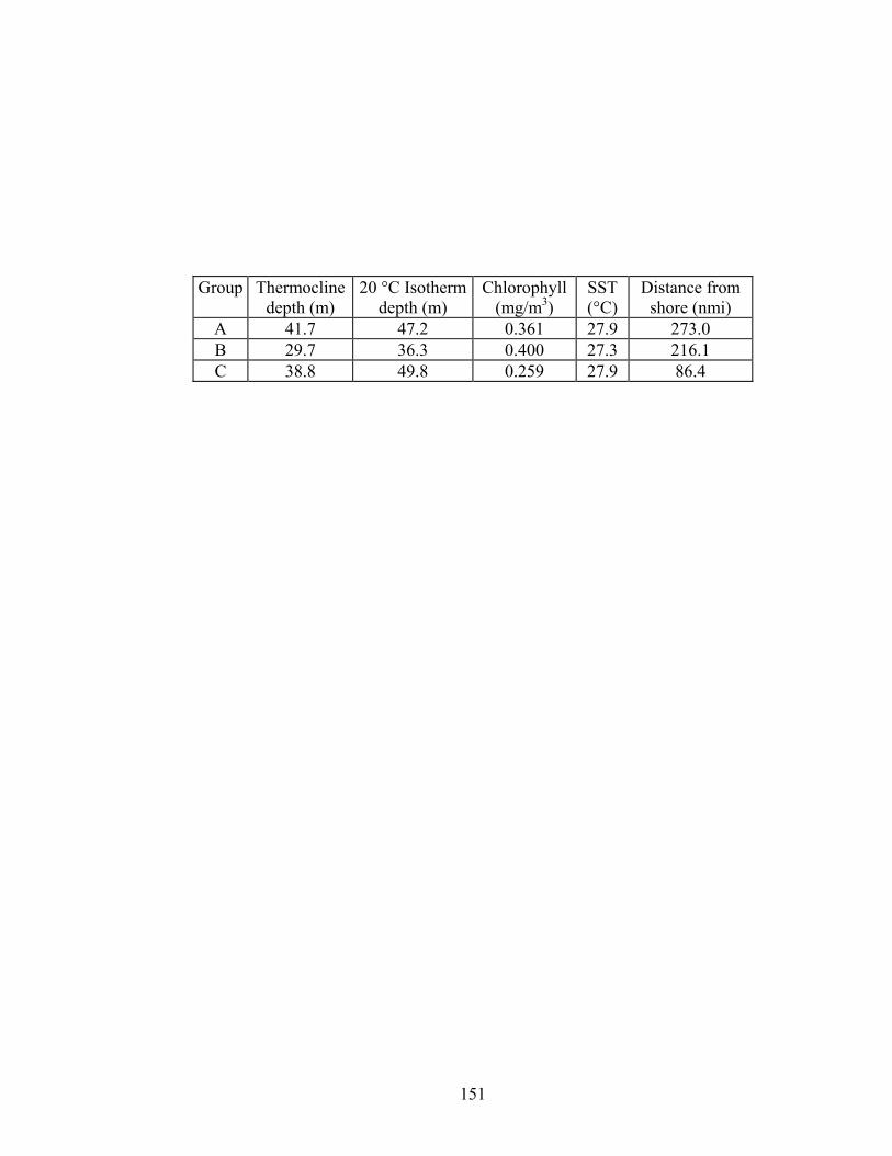
Group Thermocline depth (m)
20 °C Isotherm depth (m)
Chlorophyll (mg/m3)
SST (°C)
Distance from shore (nmi)
A 41.7 47.2 0.361 27.9 273.0 B 29.7 36.3 0.400 27.3 216.1 C 38.8 49.8 0.259 27.9 86.4
151

152
Figure 26. Interaction plot of mean total length with time period and group
membership. Numbers in parentheses indicate sample size; error bars represent
standard error of the mean.

.
182
184
186
188
190
192
194
196
198
200
202
1973-74 1988-89
Time Period
Group BGroup C
(19)
(46)
(14)
(36)
Mea
n To
tal L
engt
h (c
m)
153

interactions between group and time (F1,79 = 1.6863, P = 0.1980). Back-
calculated birth dates were not significantly different from a uniform distribution
for both groups B (K = 0.75, P > 0.10) and C (K = 0.30, P > 0.10), indicating no
difference in seasonality of female reproduction (Figure 27).
Discussion
A priori groups
Stratifying data according to oceanographic variables through the use of
PCA and k-means cluster analysis provided a framework for spatial comparisons
based on habitat. The application could easily be extended for comparing genetic,
morphometric, and life history characteristics of other marine species that inhabit
diverse oceanographic regions. This method could be used for developing a
priori groups for developing potential stock designations if animals occur in
oceanographic regions that could effectively limit animal movement.
Alternatively, it could be used for developing finer scale strata for examining
clinal differences by increasing the number of groups specified in the k-means
cluster analysis.
Spatial and temporal comparisons
Why sexually mature females in group B were different in total length
from group C in the “early” years and total length in group B mature females
changed over time cannot be determined. However, three hypotheses could
explain the differences: (1) movement of animals due to environmental changes,
(2) morphological change in response to environmental changes, and (3) sampling
biases.
154

155
Figure 27. Back-projected birth date distributions for groups B and C.
Cumulative back-projected birth date distributions are not significantly different
from a uniform cumulative distribution for groups B and C. Bars indicate
frequency of birth dates; points indicate observed and expected cumulative
proportions.

Cum
ulat
ive
Prop
ortio
nC
umul
ativ
e Pr
opor
tion
)
(Group B)
0.0
0.2
0.4
0.6
0.8
1.0
JAN
FEB
MA
R
APR
MA
Y
JUN
JUL
AU
G
SEP
OC
T
NO
V
DEC
Month
0
2
4
6
8
10
12
14
Freq
uenc
y
ObservedExpected
n=80
(Group C
156
0.0
0.2
0.4
0.6
0.8
1.0
JAN
FEB
MA
R
APR
MA
Y
JUN
JUL
AU
G
SEP
OC
T
NO
V
DEC
Month
012345678910
Freq
uenc
y
ObservedExpected
n=20

Movement of animals due to environmental change
Groups B and C could be distinct subpopulations within central D.
delphis, and the apparent increase in length over time of group B may be due to
movement of the longer group C animals into their habitat. In fact, a decrease in
the abundance of the northern stock of D. delphis in the ETP and a concomitant
increase off southern California, starting in the late 1970s, suggests a large-scale
shift in the distribution of D. delphis may have occurred in the eastern North
Pacific (Anganuzzi and Buckland 1994). During the time of this hypothesized
shift in distribution, a cool to warm oceanographic regime shift occurred in the
North Pacific during the winter of 1976-77. These changes were also apparent,
although to a lesser degree, in the warm pool area of the ETP, where central D.
delphis occur (Fiedler 2002b). This regime shift could have prompted a shift in
distribution of D. delphis within the region. Either group C animals replaced
group B as these animals moved elsewhere, or group C animals mixed with group
B, melding the once distinct subpopulations into one.
Another possibility is that sampling in the “early” years captured a
temporary distributional shift within the ETP of shorter animals from the northern
( X = 178.5;179.2 cm; (Perrin et al. 1985; Perryman and Lynn 1993)) or southern
( X = 188.5;184.3 cm; (Perrin et al. 1985; Perryman and Lynn 1993)) stocks in
response to the 1972-73 El Niño-Southern Oscillation (ENSO). This is a
reasonable hypothesis because D. delphis have been documented to shift their
distribution interannually in response to ENSO events in the ETP (Reilly and
Fiedler 1994). This shift likely occurs when the warm surface waters and deep
157

thermoclines associated with ENSO (Fiedler 2002b) reduce the habitat quality for
D. delphis. This hypothesis implies that groups B and C were not different in
average total length and that the observed difference may be an artifact of
sampling different D. delphis stocks during ENSO. The relative distance between
group B and the southern D. delphis stock is less than that between group B and
the northern stock (Figure 28), suggesting that movement of southern rather than
the northern stock animals into central stock habitat is more likely.
Although the roughly 240 nmi separating the southern stock and group B
of the central stock may seem like a lengthy distance to travel, a radio-tagged D.
delphis in the northeastern Pacific was documented traveling 270 nmi from its
capture site (Evans 1975). Not only have D. delphis been documented traveling
similar distances, but a shift in distribution greater than that proposed above was
observed in 1987. Reilly and Fiedler (1994) reported that southern D. delphis
only occurred in the far east off South America during the ENSO of 1987,
whereas in La Niña conditions their range extended out to 110º W. If “far east” is
assumed to be 85º W, then the distance that animals may have traveled between
these distributions is roughly 1500 nmi. Using thermocline depth as an index of
D. delphis upwelling habitat, during ENSO favorable conditions contracted
eastward and southward at the equator and changed very little at the Costa Rica
Dome (Figure 29). Thus, it is quite likely that individuals from the northern or
southern stocks of D. delphis might travel to the area of the Costa Rica Dome in
search of favorable conditions during ENSO.
158

159
Figure 28. Relative distance (indicated by arrows) between the northern and
southern stocks and group C of the central stock. Data points are D. delphis
sightings from SWFSC cruises. Lines surrounding data points indicate the
management units to which these sightings would belong.

160
-150 -140 -130 -120 -110 -100 -90 -80-20
-10
0
10
20
30
southern
central
northern

161
Figure 29. ENSO effect on thermocline depth (-2 x linear fit to Southern
Oscillation Index). Orange and blue areas indicate deepening and shoaling of the
thermocline, respectively. Figure taken from Fiedler and Talley (in press).

162

Morphological change in response to evironmental change
If a shift in distribution did not occur, another hypothesis is that the
observed change in total length for group B stemmed from a change in habitat and
prey type and availability. The notion that length changed during such a short
time period as the 1972-1973 ENSO is biologically impossible. A change in total
body length over time, in response to a regime shift, is more of a possibility.
However, why would group C and not group B change? The only explanation for
this would be if the habitat of group B changed and that of group C did not. To
examine this possibility, the distribution of surface chlorophyll change between
pre-and post-regime shift years in the study area was inspected. Groups B and C
both inhabited areas of zero and positive chlorophyll change (Figure 30).
Considering that spatial and seasonal sampling differences between pre- and post-
regime periods in the chlorophyll data exist and inconclusive spatial patterns in
chlorophyll change were found, the above explanation seems unlikely.
Sampling biases
Potential sampling biases associated with by-caught dolphins in the tuna
purse-seine fishery in the ETP abound and have been discussed in several papers
(Perrin et al. 1976a; Barlow 1985; Perrin et al. 1985; Chivers and Myrick 1993;
Archer et al. 2001). Three potential biases that were not removed through data
stratification and their relation to this study will be discussed here: sampling
methods, age structure, and number of dolphins killed per set.
Sampling protocol remained constant during the years of this study (1973-
1993). The only difference in sampling design was that in 1973 vessel
163

164
Figure 30. Mean surface chlorophyll change (mg/m3) between pre- and post-
regime shift years (1980-1999)/(1955-1975). Symbols represent a priori group
samples. Green coloration indicates positive change, yellow indicates no change,
and blue indicates negative change in post-regime years. Darker colors indicate
greater change. Chlorophyll data courtesy of Paul Fiedler, SWFSC.
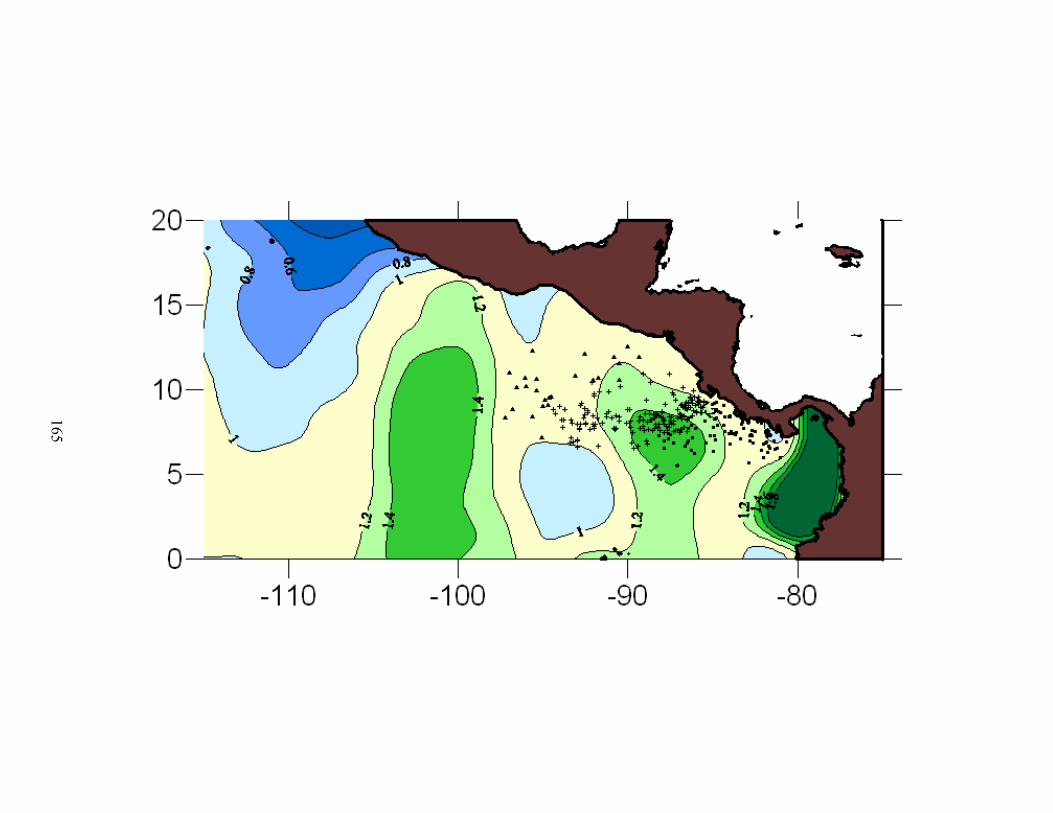
165

Participation in the tuna observer program was voluntary, whereas starting in
1974 it was mandatory (Barlow 1985). Length and age measures are not likely to
be effected by random vs. non-random vessel participation. Changes in the way
total body length measurements were taken would be the only potential sampling
protocol factor to bias the results of this study and there is no evidence of change
in methods or equipment.
Perrin et al. (1985) addressed the possibility that differences in body
length may be biased by differences in age structure (i.e., sampling young mature
females would result in smaller mean lengths), but the mean age of mature
females is constant across groups and time periods in this study and therefore not
a likely source of bias to explain the differences in length found in this study.
Another potential source of bias is the number of dolphins killed per set. The
proportion of mature female northern S. attenuata was found to depend
significantly on this variable (Barlow 1985). Barlow suggested that this
association may be due to animals segregating by reproductive maturity and that
vulnerability to high kill-per-set varies by maturity status. According to this
rationale, parameters associated with only mature females would not be impacted
by this bias, and therefore would not be of concern in this study.
The most likely explanation for the observed differences in length over
time and space is that of a temporary shift in distribution during the ENSO of
1972-73. If this is the case, there is no evidence for additional subpopulations
within central D. delphis. The lack of seasonality in both groups also supports
this. However, the existence of subpopulations has not been disproved. Potential
166

biases and data stratification led to small sample sizes that inhibited exploring the
data further. If samples become available in future years, further examination of
life history data as well as genetic markers between the hypothesized populations
A, B, and C would still be merited, considering the dynamic oceanography within
this region.
If in fact there is movement between D. delphis stocks during ENSO
events, there are implications for the stocks themselves and for estimates of
growth and reproduction for central D. delphis. Mixing of stocks during ENSO
events could increase the genetic diversity of the respective populations as well as
provide potential colonists to central D. delphis. If a severe reduction in
population abundance occurred, these colonists could make the central stock more
resilient to such disturbances. However, movement of animals between stock
boundaries also brings into question the meaning of “stock”. Is there gene flow
between D. delphis stocks during ENSO and is it large and frequent enough to
negate their stock designations that were based on the idea that they are
reproductively isolated? Genetic markers for all three stocks need to be looked at
in addition to examining the life history of the northern and southern stocks to
determine whether they are maintaining a large degree of reproductive isolation.
Estimates of growth and reproduction of central D. delphis such as ELB,
LSM, and dates of births (Chapter 4) would effectively be averaged by the
inclusion of shorter animals from the northern or southern stocks for some years.
However, the degree and direction in which these parameters would be changed
cannot be known since the number of animals moving during ENSO events or
167

which stock they are coming from are not known. Removal of samples collected
during ENSO years could limit this potential bias. However, this would reduce
sample size by hundreds and would not be recommended unless additional data
become available to support the hypothesis that D. delphis stocks mix during
ENSO events.
168

CHAPTER 6: CONCLUSIONS
The goals of this study were a) to determine if age estimations of
delphinid teeth could be improved or maintained using enhanced digital imaging,
b) to describe the growth and reproduction of central female D. delphis, and c) to
determine whether spatial and or temporal trends in total length and calving
season of central females were apparent in the ETP (potentially reflecting finer
scale population structure).
My comparison of precision and bias between two aging platforms
(Chapter 3) provided encouraging results for using digital imaging for aging but
also pointed to inherent flaws in the protocol that require further investigation.
Precision of age estimates obtained using the compound microscope and the
image analyzer were comparable. However, age estimates of older animals were
lower for one reader when using the image analyzer. This likely occurred because
the reader did not consistently use higher objective images to read the last group
of GLGs. Replicate experiments with new readers and improved protocols are
currently being conducted to determine whether this bias can be resolved. If this
bias can be eliminated, the image analyzer would serve as an excellent tool in
archiving and reading delphinid teeth.
Analyses of growth and reproductive parameters show that central female
D. delphis (Chapter 4) have different life history characteristics than their
conspecifics in the North Pacific and from the closely related Stenella spp. in the
ETP. Geographic variation in the North Pacific appears to occur in D. delphis,
with longer individuals and year-round breeding found in the south. Central D.
169
delphis also appear to be unique in comparison to the closely related Stenella spp.
in the ETP because they have a calving interval that is approximately one year
shorter. This is likely due to the greater number of females that lactate while
pregnant. D. delphis may be able to handle the increased energy demands of
lactating while pregnant due to the upwelling modified habitat that they inhabit
which likely provides a richer food source than the relatively unproductive areas
that Stenella spp. inhabit.
Several caveats to life history parameter estimations associated with
fishery sampling were noted during the analysis of growth and reproduction and
alternative estimates were presented based on these caveats. ELB could be
overestimated by 3.4 cm due to undocumented calf mortality, ASM could be
underestimated by two years due to “missing” immature animals in the sample,
and calving interval could be underestimated by a factor of 1.7 due to high fetal
mortality possibly associated with repeated chase and capture in the fishery.
These alternative estimates must be considered if these parameters are to be used
in population modeling for this species as well as other species impacted by the
same fishery.
The spatial and temporal analysis (Chapter 5) showed that central D.
delphis habitat varies, and although evidence for finer scale population structure
was not found, there was evidence that animals may move considerable distances
and possibly cross stock boundaries in response to changes in habitat. The mean
total body length of D. delphis sampled “on” the Costa Rica Dome was 10 cm
shorter than those sampled “off” the Costa Rica Dome during the years 1973-74.
170

However, no difference in mean total body length between the aforementioned
spatial groups was apparent in the “later” years of 1988-89. The difference
between spatial groups within the central stock during the 1973-74 time period
might be attributed to shorter southern stock D. delphis moving into the higher
quality habitat of the Costa Rica Dome area during the strong El Nino of 1972-73
when preferred habitat was likely reduced in the south. There is no evidence for
finer scale population structure in central female D. delphis in the data analyzed,
and the most likely explanation of results point to a temporary distribution shift of
animals rather than a biological difference between animals “on” and “off” the
Dome.
In summary, image analysis appears to be a promising tool for aging
delphinid teeth that needs to be explored further. There is no evidence for fine
scale geographic variation in life history within the central stock, although
individuals appear to cross stock boundaries in response to environmental change.
Furthermore, large scale geographic variations in life history characteristics of D.
delphis in the North Pacific was documented with longer individuals and year-
round breeding found in the tropics.
171

LITERATURE CITED
Akin, P. A., K. M. Peltier, and R. B. Miller. 1993. Techniques for the preparation
and examination of reproductive samples collected from dolphins in the
eastern tropical Pacific. NOAA Technical Memorandum NMFS-SWFSC-
192, U.S. Department of Commerce, 26 pp.
Anganuzzi, A. A. and S. Buckland. 1994. Relative abundance of dolphins
associated with tuna in the eastern Pacific Ocean: Analysis of 1992 data.
Report of the International Whaling Commission 44: 361-366.
Archer, F., T. Gerrodette, A. Dizon, K. Abella, and S. Southern. 2001.
Unobserved kill of nursing dolphin calves in a tuna purse-seine fishery.
Marine Mammal Science 17: 540-554.
Au, D. W. K. and W. L. Perryman. 1985. Dolphin habitats in the eastern tropical
Pacific. Fishery Bulletin, U.S. 83: 623-643.
Barlow, J. 1984. Reproductive seasonality in pelagic dolphins (Stenella spp.):
implications for measuring rates. Report of the International Whaling
Commission (Special Issue 6): 191-198.
Barlow, J. and A. A. Hohn. 1984. Interpreting spotted dolphin age distributions.
NOAA Technical Memorandum NMFS-SWFC-48, U.S. Department of
Commerce, 22 pp.
Barlow, J. 1985. Variability, trends, and biases in reproductive rates of spotted
dolphins, Stenella attenuata. Fishery Bulletin 83: 657-669.
172

Bayliff, W. H., editor. 2002. Annual Report of the Inter-American Tuna
Commission, 2000. Inter-American Tropical Tuna Commission, La Jolla,
171 pp.
Bengtson, J. L. and R. M. Laws. 1985. Trends in crabeater seal age at maturity:
An insight into Antarctic marine interactions. Pp. 669-675 in Antarctic
nutrient cycles and food webs (R. M. Laws, ed.). Springer-Verlag, Berlin.
Bernt, K. E., M. O. Hammill, and K. M. Kovacs. 1996. Age estimation of grey
seals (Halichoerus grypus) using incisors. Marine Mammal Science 12:
476-482.
Best, P. B. 2001. Distribution and population separation of Bryde's whale
Balaenoptera edeni off southern Africa. Marine Ecology Progress Series
220: 277-289.
Boyd, I. L., C. Lockyer, and H. D. Marsh. 1999. Reproduction in marine
mammals. Pp. 218-286 in Biology of Marine Mammals (S. A. Rommel,
ed.). Smithsonian Institution Press, Washington, D.C.
Bronson, F. H. 1989. Mammalian reproductive biology. The University of
Chicago Press, Chicago.
Caillet, G. M., L. Botsford, J. G. Brittnacher, G. Ford, M. Matsubayashi, A. King,
D. Watters, and R. G. Kope. 1996. Development of a computer-aided age
determination system: evaluation based on otoliths of bank rockfish off
California. Transactions of the American Fisheries Society 125: 874-888.
173
Campana, S. E., M. C. Annand, and J. I. McMillan. 1995. Graphical and statistical
methods for determining the consistency of age determinations.
Transactions of the American Fisheries Society 124: 131-138.
Chang, W. Y. B. 1982. A statistical method for evaluating the reproducibility of
age determination. Canadian Journal of Fisheries and Aquatic Sciences
39: 1208-1210.
Chavez, F. P. and R. T. Barber. 1987. An estimate of new production in the
equatorial Pacific. Deep-Sea Research 34: 1229-1243.
Chivers, S. J. and A. C. Myrick, Jr. 1993. Comparison of age at sexual maturity
and other reproductive parameters for two stocks of spotted dolphin,
Stenella attenuata. Fishery Bulletin 91: 611-618.
Chivers, S. J. and D. P. DeMaster. 1994. Evaluation of biological indices for three
eastern Pacific dolphin species. Journal of Wildlife Management 58: 470-
478.
Chivers, S. J., K. M. Robertson, and M. D. Henshaw. 1997. Composition of the
incidental kill of cetaceans in two California gillnet fisheries: 1990-1995.
Report of the International Whaling Commission: 909-915.
Chivers, S. J. 2002a. Cetacean life history. Pp. 221-225 in Encyclopedia of
Marine Mammals (J. G. M. Thewissen, ed.). Academic Press, San Diego.
Chivers, S. J. 2002b. Age structure of female eastern spinner dolphins (Stenella
longirostris orientalis) incidentally killed in the eastern tropical Pacific
tuna purse-seine fishery. Administrative Report LJ-02-11, Southwest
174

Fisheries Science Center, National Marine Fisheries Service, La Jolla, 10
pp.
Collet, A. and H. St. Girons. 1984. Preliminary study of the male reproductive
cycle in common dolphins, Delphinus delphis, in the Eastern North
Atlantic. Report of the International Whaling Commission (Special Issue
6): 355-360.
Cox, D. and E. Snell. 1989. Analysis of binary data, 2nd edition. Chapman and
Hall, London.
DeMaster, D. P. 1978. Calculation of the average age at sexual maturity in marine
mammals. Journal of the Fisheries Research Board of Canada 35: 912-
930.
Dizon, A. E., W. F. Perrin, and P. A. Akin. 1994. Stocks of dolphins (Stenella
spp. and Delphinus delphis) in the eastern tropical Pacific: a
phylogeographic classification. NOAA Technical Report NMFS 119, U.S.
Department of Commerce, 20 pp.
Douglas, M. E., G. D. Schnell, and D. J. Hough. 1984. Differentiation between
inshore and offshore spotted dolphins in the eastern tropical Pacific
Ocean. Journal of Mammology 65: 375-387.
Eberhardt, L. and D. Siniff. 1977. Population dynamics and marine mammal
management policies. Journal of the Fisheries Research Board of Canada
34: 183-189.
175

Eberhardt, L. L. 1977. Optimal policies for conservation of large mammals, with
special reference to marine ecosystems. Environmental Conservation 4:
205-212.
Evans, K., M. A. Hindell, K. Robertson, C. Lockyer, and D. Rice. 2002. Factors
affecting the precision of age determination of sperm whales (Physeter
macrocephalus). Journal of Cetacean Research and Management 4: 193-
201.
Evans, W. E. 1975. Distribution, differentiation of populations, and other aspects
of the natural history of Delphinus delphis Linnaeus in the northeastern
Pacific. Ph.D thesis. University of California at Los Angeles, Los Angeles.
Evans, W. E. 1982. Distribution and differentiation of stock of Delphinus delphis
Linnaeus in the northeastern Pacific. Pp. 45-66 in Mammals in the Seas.
FAO, Rome.
Evans, W. E. 1994. Common Dolphin, White-bellied Porpoise Delphinus delphis
Linnaeus, 1758. Pp. 191-224 in Handbook of Marine Mammals, Volume
5: The First Book of Dolphins (R. Harrison, ed.). Academic Press,
London.
Ferrero, R. C. and W. A. Walker. 1993. Growth and reproduction of the northern
right whale dolphin, Lissodelphis borealis, in the offshore waters of the
North Pacific Ocean. Canadian Journal of Zoology 71: 2335-2344.
Ferrero, R. C. and W. A. Walker. 1994. Growth and reproduction of the common
dolphin, Delphinus delphis, in the offshore waters of the north Pacific
Ocean. Fishery Bulletin 93: 483-494.
176
Ferrero, R. C. and W. A. Walker. 1996. Age, growth, and reproductive patterns of
the Pacific white-sided dolphin (Lagenorhynchus obliquidens) taken in
high seas drift nets in the central North Pacific Ocean. Canadian Journal of
Zoology 74: 1673-1687.
Fiedler, P. C. 1994. Seasonal and interannual variability of coastal zone scanner
phytoplankton pigments and winds in the eastern tropical Pacific. Journal
of Geophysical Research - Oceans 99: 18,371-18,384.
Fiedler, P. C. and S. B. Reilly. 1994. Interannual variability of dolphin habitats in
the eastern tropical Pacific: effects on abundance estimated from tuna
vessel sightings, 1975-1990. Fishery Bulletin 92: 451-463.
Fiedler, P. C. 2002a. The annual cycle and biological effects of the Costa Rica
Dome. Deep Sea Research I 49: 321-338.
Fiedler, P. C. 2002b. Environmental change in the eastern tropical Pacific Ocean:
review of ENSO and decadal variability. Marine Ecology Progress Series
244: 265-283.
Fiedler, P. C. and L. D. Talley. 2004. Hydrography of the eastern tropical Pacific:
A review. Progress in Oceanography submitted.
Fiedler, P. C. and L. D. Talley. In press. Hydrography of the eastern tropical
Pacific: A review. Progress in Oceanography.
Ford, J. K. B. 2001. Killer Whale. Pp. 669-676 in Encyclopedia of Marine
Mammals (B. Wursig, ed.). Academic Press, San Diego.
177
Forney, K. A. and J. Barlow. 1998. Seasonal patterns in the abundance and
distribution of California cetaceans, 1991-1992. Marine Mammal Science
14: 460-489.
Fowler, C. W. 1981. Density dependence as related to life history strategy.
Ecology 62: 602-610.
Fowler, C. W. 1987. A review of density dependence in populations of large
mammals. Pp. 401-441 in Current Mammology (H. H. Genoways, ed.).
Plenum Publishing Corporation, New York, London.
Goren, A. D., P. F. Brodie, S. Spotte, G. C. Ray, H. W. Kaufman, A. J. Gwinnet,
J. J. Sciubba, and J. D. Buck. 1987. Growth layer groups (GLGs) in the
teeth of an adult belukha whale (Delphinapterus leucas) of known age:
evidence for two annual layers. Marine Mammal Science 3: 14-21.
Gurevich, V. S., B. S. Stewart, and L. H. Cornell. 1980. The use of tetracycline in
age determination of common dolphins, Delphinus delphis. Report of the
International Whaling Commission (Special Issue 3): 165-169.
Hall, M. A. 1998. An ecological view of the tuna-dolphin problem: impacts and
trade-offs. Reviews in Fish Biology and Fisheries 8: 1-34.
Hansen, D. V. and A. Herman. 1988. A seasonal isotherm depth climatology for
the eastern tropical Pacific. NOAA Technical Report ERL-434-AOML 33,
U.S. Department of Commerce, 35 pp.
Harrison, R. J., R. C. Boice, and R. L. Brownell, Jr. 1969. Reproduction in wild
and captive dolphins. Nature 222: 1143-1147.
178

Harrison, R. J., R. L. Brownell, Jr., and R. C. Boice. 1972. Reproduction and
gonadal appearances in some odontocetes. Pp. 409-419 in Functional
Anatomy of Marine Mammals (R. J. Harrison, ed.). Academic Press,
London.
Henderson, J. R., W. F. Perrin, and R. B. Miller. 1980. Rate of gross annual
production in dolphin populations (Stenella spp. and Delphinus delphis) in
the eastern tropical Pacific, 1973-1978. Administrative Report LJ-80-02,
Southwest Fisheries Science Center, National Marine Fisheries Service,
La Jolla, 51 pp.
Heyning, J. E. and W. F. Perrin. 1994. Evidence for two species of common
dolphins (genus Delphinus) from the eastern north Pacific. Contributions
in Science 442: 1-35.
Hobbs, R. C. and L. L. Jones. 1993. Impacts of high seas driftnet fisheries on
marine mammal populations in the North Pacific. International North
Pacific Fisheries Commission Bulletin 53: 409-434.
Hofmann, E. E., A. J. Busalacchi, and J. J. O'Brien. 1981. Wind generation of the
Costa Rica Dome. Science 214: 552-553.
Hohn, A. A. 1980a. Analysis of growth layers in teeth of Tursiops truncatus using
light microscopy, microradiography, and SEM. Report of the International
Whaling Commission (Special Issue 3): 155-160.
Hohn, A. A. 1980b. Age determination and age-related factors in the teeth of
western North Atlantic bottlenose dolphins. Scientific Reports of the
Whales Research Institute, Tokyo 32: 39-66.
179

Hohn, A. A. and P. S. Hammond. 1983. Growth in the first year of the offshore
spotted dolphin, Stenella attenuata, in the eastern tropical Pacific.
Administrative Report LJ-83-08, Southwest Fisheries Science Center,
National Marine Fisheries Service, La Jolla, 33 pp.
Hohn, A. A. and P. S. Hammond. 1985. Early postnatal growth of the spotted
dolphin, Stenella attenuata, in the offshore eastern tropical Pacific.
Fishery Bulletin 83: 553-566.
Hohn, A. A. 1989. Variation in life-history traits: the influence of introduced
variation. Ph.D. thesis. University of California at Los Angeles, Los
Angeles.
Hohn, A. A., M. D. Scott, R. S. Wells, J. C. Sweeney, and A. B. Irvine. 1989.
Growth layers in teeth from known-age, free-ranging bottlenose dolphins.
Marine Mammal Science 5: 315-342.
Hohn, A. A. and S. Fernandez. 1999. Biases in dolphin age structure due to age
estimation technique. Marine Mammal Science 15: 1124-1132.
Hohn, A. A. 2002. Age estimation. Pp. 6-13 in Encyclopedia of Marine Mammals
(J. G. M. Thewissen, ed.). Academic Press, San Diego.
Hugget, A. S. G. and W. F. Widdas. 1951. The relationship between mammalian
foetal weight and conception age. Journal of Physiology 114: 306-317.
Hui, C. A. 1977. Data preparation and analysis for studies on growth and
reproduction of Delphinus in the eastern tropical Pacific. Southwest
Fisheries Center Contract Report PO-01-6-200-11439, 14 pp.
180

Hui, C. A. 1979a. Correlates of maturity in the common dolphin, Delphinus
delphis. Fishery Bulletin 77: 295-300.
Hui, C. A. 1979b. Undersea topography and distribution of dolphins of the genus
Delphinus in the southern California Bight. Journal of Mammalogy 60:
521-527.
Hui, C. A. 1980. Variability of dentin deposits in Tursiops truncatus. Canadian
Journal of Fisheries and Aquatic Sciences 37: 712-716.
Jefferson, T. A. and K. Van Waerebeek. 2002. The taxonomic status of the
nominal dolphin species Delphinus tropicalis Van Bree, 1971. Marine
Mammal Science 18: 787-818.
Kasuya, T. 1985. Effect of exploitation on reproductive parameters of the spotted
and striped dolphins off the Pacific coast of Japan. Scientific Reports of
the Whales Research Institute, Tokyo 36: 107-138.
Kessler, W. S. 1990. Observations of long rossby waves in the northern tropical
Pacific. Journal of Geophysical Research 95 (C4): 5183-5217.
Kleinenberg, S. E. 1956. Mlekopitauishchenie Chernogo i Azovskogo Morei.
(Mammals of the Black Sea and Sea of Azov). Izdatel'stvo Akademi Nauk
SSSR, Moscow.
Klevezal, G. A. 1980. Layers in the hard tissues of mammals as a record of
growth rhythms of individuals. Report of the International Whaling
Commission (Special Issue 3): 89-94.
181

Klevezal, G. A. and A. C. Myrick, Jr. 1984. Marks in tooth dentine of female
dolphins (Genus Stenella) as indicators of parturition. Journal of
Mammology 65: 103-110.
Laidig, T. E. and D. E. Pearson. 1992. Documentation of three computer
programs used to assess daily age from the hard structures of animals.
Technical Memorandum NMFS-SWFSC-168, Department of Commerce,
168 pp.
Laird, A. K. 1969. The dynamics of growth. Research/Development 20: 28-31.
Laws, R. M. 1956. Growth and sexual maturity in aquatic mammals. Nature 178:
193-194.
Laws, R. M., I. S. C. Parker, and R. C. B. Johnstone. 1975. Elephants and their
habitats: The ecology of elephants in North Buryovo, Uganda. Clarendon
Press, Oxford.
Lawson, J. W., G. D. Harrison, and W. D. Bowen. 1992. Factors affecting
accuracy of age determination in the harp seal, Phoca groenlandica.
Marine Mammal Science 8: 169-171.
Lennert, C. and M. A. Hall. 1995. Estimates of incidental mortality of dolphins in
the eastern Pacific Ocean tuna fishery in 1993. Report of the International
Whaling Commission 45: 387-390.
Lockyer, C. 1984. Review of baleen whale (Mysteceti) reproduction and
implications for management. Report of the International Whaling
Commission (Special Issue 6): 27-50.
182

Lockyer, C. and J. Sigurjonsson. 1992. The Icelandic fin whale, (Balaenoptera
physlaus): biological parameters and their trends over time. Report of the
International Whaling Commission 42: 617-618.
Lockyer, C. 1995. Investigation of aspects of the life history of the harbour
porpoise, Phocoena phocoena, in British waters. Report of the
International Whaling Commission (Special Issue 16): 189-197.
Lockyer, C. H. 1990. The importance of biological parameters in population
assessments with special reference to fin whales from the N.E. Atlantic.
North Atlantic Studies 2: 22-31.
Manzanilla, S. R. 1989. The 1982-1983 El Niño event recorded in dentinal growth
layers in teeth of Peruvian dusky dolphins (Lagenorhyncus obscurus).
Canadian Journal of Zoology 67: 2120-5.
Marsh, H. and T. Kasuya. 1984. Changes in the ovaries of the short-finned piliot
whale, Globicephala macrorhyncus, with age and reproductive activity.
Report of the International Whaling Commission (Special Issue 6): 311-
335.
Martin, A. R. and P. Rothery. 1993. Reproductive parameters of female long-
finned pilot whales (Glocicephala melas) around the Faroe Islands. Report
of the International Whaling Commission (Special Issue 14): 263-304.
Mattiucci, S., P. Abaunza, L. Ramadori, and G. Nascetti. 2004. Genetic
identification of Anisakis larvae in European hake from Atlantic and
Mediterranean waters for stock recognition. Journal of Fish Biology 65:
495-510.
183

McCreary, J. P., H. S. Lee, and B. B. Enfield. 1989. The response of the coastal
ocean to strong offshore winds: with application to circulations in the
Gulfs of Tehuantepec and Papagayo. Journal of Marine Research 47: 81-
109.
Murphy, S. 2004. The biology and ecology of the short-beaked common dolphin
Delphinus delphis in the North-east Atlantic. Ph.D. thesis. National
University of Ireland, Cork.
Myrick, A. C., Jr. 1980. Examination of layered tissues of odontocetes for age
determination using polarized light microscopy. Report of the
International Whaling Commission (Special Issue 3): 105-112.
Myrick, A. C., Jr, E. W. Shallenberger, I. Kang, and D. B. MacKay. 1984.
Calibration of dental layers in seven captive Hawaiian spinner dolphins,
Stenella longirostris, based on tetracycline labeling. Fishery Bulletin 82:
207-225.
Myrick, A. C., Jr and L. H. Cornell. 1990. Calibrating dental layers in captive
bottlenose dolphins from serial tetracycline labels and tooth extractions.
Pp. 587-608 in The Bottlenose dolphin (R. R. Reeves, ed.). Academic
Press, Inc., San Diego.
Myrick, A. C., Jr , A. A. Hohn, J. Barlow, and P. A. Sloan. 1986. Reproductive
biology of female spotted dolphins, Stenella attenuata , from the eastern
tropical Pacific. Fishery Bulletin 84: 247-259.
Myrick, A. C., Jr., A. A. Hohn, P. Sloan, M. Kimura, and D. Stanley. 1983.
Estimating age of spotted and spinner dolphins (Stenella attenuata and
184

Stenella longirostris) from teeth. NOAA Technical Memorandum NMFS-
SWFC-30, U.S. Department of Commerce, 17 pp.
Neal, P. R. 1987. Automated aging of Pacific halibut (Hippoglossus stenolepsis)
otoliths using digital image analysis. Master's thesis. University of
Washington, Seattle.
Neumann, D. R. 2001. Seasonal movements of short-beaked common dolphins
(Delphinus delphis) in the north-western Bay of Plenty, New Zealand:
influence of sea surface temperature and El Niño/La Niña. New Zealand
Journal of Marine and Freshwater Research 35: 371-374.
Olesiuk, P. F., M. A. Bigg, and G. M. Ellis. 1990. Life history and population
dynamics of resident killer whales (Orcinus orca) in the coastal waters of
British Columbia and Washinton state. Report of the International
Whaling Commission (Special Issue 12): 209-243.
Oosthuizen, W. and M. Bester. 1997. Comparison of age determination
techniques for known-age Cape fur seals. South African Journal of
Zoology 32: 106-111.
Orban, B. J. 1976a. Dentin. Pp. 105-140 in Orban's Oral Histology and
Embryology (S. N. Bhaskar, ed.). Mosby, Saint Louis.
Orban, B. J. 1976b. Cementum. Pp. 182-205 in Orban's Oral Histology and
Embryology (S. N. Bhaskar, ed.). Mosby, Saint Louis.
Osnes-Erie, L. 1999. Food habits of common dolphin (Delphinus delphis and D.
capensis) off California. Master of Science. San Jose State University.
Perrin, W. F. 1969. Using porpoise to catch tuna. World Fishing 18: 42-45.
185

Perrin, W. F. 1970. The problem of porpoise mortality in the U.S. tropical tuna
fleet. Pp. 45-48 in Proceedings of the 6th Conference on Biological Sonar
and Diving Mammals. Stanford Research Institute.
Perrin, W. F., J. M. Coe, and J. R. Zweifel. 1976a. Growth and reproduction of
the spotted porpoise, Stenella attenuata, in the offshore eastern tropical
Pacific. Fishery Bulletin 74: 229-269.
Perrin, W. F., R. B. Miller, and P. A. Sloan. 1976b. Reproductive parameters of
the offshore spotted dolphin, a geographical form of Stenella attenuata, in
the eastern tropical Pacific, 1973-75. Fishery Bulletin 75: 629-633.
Perrin, W. F., D. B. Holts, and R. B. Miller. 1977. Growth and reproduction of the
eastern spinner dolphin, a geographical form of Stenella longirostris in the
eastern tropical Pacific. Fishery Bulletin 75: 725-750.
Perrin, W. F. and A. C. J. Myrick. 1980. Report of the workshop. Report of the
International Whaling Commission (Special Issue 3): 1-50.
Perrin, W. F. and G. P. Donovan. 1984. Report of the Workshop. Report of the
International Whaling Commission (Special Issue 6): 1-24.
Perrin, W. F. and J. R. Henderson. 1984. Growth and reproductive rates in two
populations of spinner dolphins, Stenella longirostris, with different
histories of exploitation. Report of the International Whaling Commission:
417-430.
Perrin, W. F. and S. B. Reilly. 1984. Reproductive parameters of dolphins and
small whales of the family Delphinidae. Report of the International
Whaling Commission (Special Issue 6): 97-133.
186

Perrin, W. F., M. D. Scott, G. J. Walker, and V. L. Cass. 1985. Review of
geographical stocks of tropical dolphins (Stenella spp. and Delphinus
delphis) in the eastern Pacific. NOAA Technical Report NMFS 28, U.S.
Department of Commerce, 28 pp.
Perrin, W. F., G. P. Donovan, and J. Barlow, editors. 1994. Gillnets and
cetaceans. Report of the International Whaling Commission (Special Issue
15), 629 pp.
Perrin, W. F., S. J. Chivers, and F. I. Archer II. 2003. Fetal mortality in dolphins
exploited by the tuna fishery. in Abstracts of the 15th Biennial Conference
on the Biology of Marine Mammals, Greensboro, NC.
Perryman, W. L. and M. S. Lynn. 1993. Identification of geographic forms of
common dolphin (Delphinus delphis) from aerial photographs. Marine
Mammal Science 9: 119-137.
Pierce, K. V. and H. Kajimura. 1980. Acid etching and highlighting for defining
growth layers in cetacean teeth. Report of the International Whaling
Commission (Special Issue 3): 99-103.
Read, A. J. 1990. Reproductive seasonality in harbour porpoises, Phocoena
phocoena, from the Bay of Fundy. Canadian Journal of Zoology 68: 284-
288.
Read, A. J. and A. A. Hohn. 1995. Life in the fast lane: the life history of harbor
porpoises from the Gulf of Maine. Marine Mammal Science 11: 423-440.
Reilly, S. B., A. A. Hohn, and A. C. Myrick, Jr. 1983. Precision of age
determination of northern offshore spotted dolphins. Technical
187

Memorandum NOAA-TM-NMFS-SWFC-35, U.S. Department of
Commerce, 27 pp.
Reilly, S. B. and J. Barlow. 1986. Rates of increase in dolphin population size.
Fishery Bulletin 84: 527-533.
Reilly, S. B. 1990. Seasonal changes in distribution and habitat differences among
dolphins in the eastern tropical Pacific. Marine Ecology Progress Series
66: 1-11.
Reilly, S. B. and P. C. Fiedler. 1994. Interannual variability of dolphin habitats in
the eastern tropical Pacific. I: Research vessel surveys, 1986-1990. Fishery
Bulletin 92: 434-450.
Reilly, S. B., P. C. Fiedler, T. Gerrodette, L. T. Ballance, R. L. Pitman, J. M.
Borberg, and R. C. Holland. 2002. Eastern tropical Pacific dolphin
habitats - interannual variability 1986-2000. Administrative Report LJ-02-
21, Southwest Fisheries Science Center, National Marine Fisheries
Service, La Jolla, 43 pp.
Reznick, D. A. and H. Bryga. 1990. Experimentally induced life-history evolution
in a natural population. Nature 346: 357-359.
Ridgway, S. H. and R. F. Green. 1967. Evidence for a sexual rhythm in male
porpoises, Lagenorhyncus obliquidens and Delphinus delphis bairdi. The
Norwegian Whaling Gazette 1: 1-8.
Robeck, T. R., B. E. Curry, J. F. McBain, and D. C. Kraemer. 1994. Reproductive
biology of the bottlenose dolphin (Tursiops truncatus) and the potential
188

application of advanced reproductive technologies. Journal of Zoo and
Wildlife Medicine 25: 321-336.
Rosel, P. E., A. E. Dizon, and J. E. Heyning. 1994. Genetic analysis of sympatric
morphotypes of common dolphins (genus Delphinus). Marine Biology
119: 159-167.
Scheffer, V. 1950. Growth layers on the teeth of pinnipedia as an indication of
age. Science 112: 309-311.
Selzer, L. A. and P. M. Payne. 1988. The distribution of white-sided
(Lagenorhyncus acutus) and common dolphins (Delphinus delphis) vs.
environmental features of the continental shelf of the northeastern United
States. Marine Mammal Science 4: 141-153.
Smith, T. D. 1979. Report of the status of porpoise stocks workshop.
Administrative Report LJ-79-41, Southwest Fisheries Science Center,
National Marine Fisheries Service, La Jolla, 120 pp.
Smith, T. D. 1983. Changes in size of three dolphin (Stenella spp.) populations in
the eastern tropical Pacific. Fishery Bulletin 81: 1-13.
Sokal, R. R. and F. J. Rohlf. 1995. Biometry, 3rd edition. W.H. Freeman and
Company, New York.
Stewart, R. E. A., B. E. Stewart, I. Stirling, and E. Street. 1996. Counts of growth
layer groups in cementum and dentine in ringed seals (Phoca hispida).
Marine Mammal Science 12: 383-401.
Tabachnik, B. G. and L. S. Fidell. 1989. Using multivariate statistics. Harper and
Row, New York.
189

Tomlin, A. G. 1957. Mammals of the U.S.S.R and adjacent countries. Izdatel'stvo
Akademi Nauk SSSR, Moscow.
Tregenza, N. J. C. and A. Collet. 1998. Common dolphin Delphinus delphis
bycatch in pelagic trawl and other fisheries in the northeast Atlantic.
Report of the International Whaling Commission 48: 453-459.
Turan, C. 2004. Stock identification of Mediterranean horse mackerel (Trachurus
mediterraneus) using morphometric and meristic characters. Ices Journal
of Marine Science 61: 774-781.
Urian, K. W., D. A. Duffield, A. J. Read, R. S. Wells, and E. D. Shell. 1996.
Seasonality of reproduction in bottlenose dolphins, Tursiops truncatus.
Journal of Mammalogy 77: 394-403.
Wade, P. R. and R. P. Angliss. 1997. Guidelines for assessing marine mammal
stocks: report of the GAMMS workshop. NOAA Technical Memorandum
NMFS-OPR-12, U.S. Department of Commerce, Silver Spring, 93 pp.
Walker, W. A. 1981. Geographical variation in morphology and biology of
bottlenose dolphins (Tursiops) in the Eastern North Pacific.
Administrative Report LJ-81-03C, Southwest Fisheries Science Center,
National Marine Fisheries, La Jolla, 52 pp.
Wells, R. S., D. J. Boness, and G. B. Rathbun. 2002. Behavior. Pp. 324-422 in
Biology of Marine Mammals (S. A. Rommel, ed.). Smithsonian Institution
Press, Washington.
190

Whitehead, H. and J. Mann. 2000. Female reproductive strategies of cetaceans.
Pp. 219-246 in Cetacean Societies (H. Whitehead, ed.). University of
Chicago Press, Chicago.
Winans, G. A., M. M. Paquin, D. M. Van Doornik, B. M. Baker, P. Thornton, D.
Rawding, A. Marshall, P. Moran, and S. Kalinowski. 2004. Genetic stock
identification of steelhead in the Columbia River Basin: An evaluation of
different molecular markers. North American Journal of Fisheries
Management 24: 672-685.
Wyrtki, K. 1964. Upwelling in the Costa Rica Dome. Fishery Bulletin 63: 355-
372.
Wyrtki, K. 1966. Oceanography of the eastern equatorial Pacific. Oceanography
and Marine Biology: An Annual Review 4: 33-68.
191

APPENDIX: LIST OF ABBREVIATIONS
APR annual pregnancy rate
ASM age at attainment of sexual maturity
CHL surface chlorophyll concentration
DIST distance from shore
ELB estimated length at birth
ENSO El Niño-Southern Oscillation
ETP eastern tropical Pacific
GLG growth layer group
LSM length at attainment of sexual maturity
MMPA Marine Mammal Protection Act
NEC North Equatorial Current
NECC North Equatorial Counter Current
NMFS National Marine Fisheries Service
PCA principal components analysis
SEC South Equatorial Current
SECC South Equatorial Counter Current
SEM scanning electron microscopy
SST sea surface temperature
SWFSC southwest fisheries science center
THERM mean thermocline depth
Z20 20 °C isotherm depth
192