graduate school of decision sciences - uni konstanz · graduate school of decision sciences . all...
TRANSCRIPT

Graduate School of Decision Sciences All processes within our society are based on decisions – whether they are individual or collective decisions. Understanding how these decisions are made will provide the tools with which we can address the root causes of social science issues. The GSDS offers an open and communicative academic environment for doctoral researchers who deal with issues of decision making and their application to important social science problems. It combines the perspectives of the various social science disciplines for a comprehensive understanding of human decision behavior and its economic and political consequences. The GSDS primarily focuses on economics, political science and psychology, but also encompasses the complementary disciplines computer science, sociology and statistics. The GSDS is structured around four interdisciplinary research areas: (A) Behavioural Decision Making, (B) Intertemporal Choice and Markets, (C) Political Decisions and Institutions and (D) Information Processing and Statistical Analysis. GSDS – Graduate School of Decision Sciences University of Konstanz Box 146 78457 Konstanz Phone: +49 (0)7531 88 3633 Fax: +49 (0)7531 88 5193 E-mail: [email protected] -gsds.uni-konstanz.de ISSN: 2365-4120 April 2017
© 2017 by the author(s)

The CAPM with Measurement Error:
There’s life in the old dog yet!∗
Anastasia Morozova†
GSDS, University of Konstanz
Winfried Pohlmeier‡
University of Konstanz, COFE, RCEA
April 24, 2017
Abstract
This paper takes a closer look on the consequences of using a market index as a proxy for
the latent market return in the capital asset pricing model. In particular, the consequences
of two major sources of misspecification are analyzed: (i) the use of inaccurate weights and
(ii) the use of only a subset of the asset universe to construct the index. The consequences
resulting from the use of a badly chosen market proxy reach from inconsistent parameter
estimates to misinterpretation of tests indicating the existence of abnormal returns.
A new minimum distance approach of estimating the CAPM under measurement error
is presented, which identifies the CAPM parameters by exploiting the cross-equation cross-
sectional restrictions resulting from a common measurement error. The new approach allows
for quantifying the impact of measurement error and for testing the presence of spurious
abnormal returns. Practical guidelines are presented to mitigate potential biases in the
estimated CAPM parameters.
Keywords: CAPM, Measurement Error, Roll’s critique, Identification, Minimum Distance
Estimation
JEL classification: G12, C58, C51, C36
∗Paper to be presented at the 3rd Konstanz-Lancaster (KoLa) workshop on Finance and Econometrics,Lancaster, May 2-3, 2017. Financial support of the first author by the Graduate School of Decision Science(GSDS) and the German Academic Exchange Service (DAAD) is gratefully acknowledged. The second authorlikes to thank Simon Benninga posthumously for a helpful discussion and for motivating him to extend his noteson measurement errors in linear systems to an application for the CAPM. All remaining errors are ours.†Department of Economics, Universitatsstraße 1, D-78462 Konstanz, Germany. Phone: +49-7531-88-2204, fax:
-4450, email: [email protected].‡Department of Economics, Universitatsstraße 1, D-78462 Konstanz, Germany. Phone: +49-7531-88-2660, fax:
-4450, email: [email protected].

Measure what is measurable, and make
measurable what is not so.
Galileo Galilei
1 Introduction
The empirical evidence supporting capital asset pricing model (CAPM) in the version of Sharpe
(1964) and Lintner (1965) is far from being convincing. Nevertheless the CAPM is still a center
piece of the asset pricing theory taught in MBA investment courses and it is still a widely used
tool among practitioners. The reasons for its failure are manifold and have launched a large
body of literature. Besides its theoretical simplicity leaving room for numerous generalizations
based on more realistic settings (multifactor models, conditional CAPM, consumption CAPM
etc.), the failure of producing convincing evidence in favor of the CAPM can also be attributed
to the difficulties of its empirical implementation. This branch of the literature has generated
numerous studies of using alternative estimation and testing procedures.1 Fama and French
(2004) offer a concise summary of the struggle to find empirical support for the CAPM.
This paper addresses the implications of using the return of a market index as a proxy for
the return of the true (equilibrium) market portfolio for the estimation of the CAPM. In a
certain sense the measurement problem can be regarded as a primary one, because the CAPM as
such is not questioned, but relates to the problem of obtaining a workable empirical framework.
The measurement problem is at the heart of the Roll’s critique (1977) who argues that the
true market portfolio includes a large range of investment opportunities including international
securities, real estate, precious metals, etc., so that the true value weighted market portfolio
is empirically elusive. In particular, he concludes (Roll (1977), p.130): ”The Theory is not
testable unless the exact composition of the true market portfolio is known and used in the
tests.” Moreover, by using market proxies due to data limitations empirical tests of the CAPM
effectively test whether the market proxies are on the minimum variance frontier.
We take different approach to Roll’s identification problem by assuming that the CAPM
holds true and investigate the properties of the CAPM in the presence of measurement problem.
By using a linear projection framework within the Sharpe-Lintner version of the CAPM we
1See Campbell et al. (1997), Chap. 5 and Jaganathan et al. (2010) for surveys on the econometric implementa-tion.
1
pick up Roll’s critique to account for the fact that the market index in empirical studies is
only a proxy that correlates more or less strongly with the true market index. This leads to an
observational model with a non-zero intercept which is observationally equivalent to a general
factor model with non-zero excess returns. Consequently, in the presence of measurement error
results of standard tests on the existence of abnormal returns, e.g. in the tradition of Gibbons
et al. (1989), render to be spurious. Our projection framework can serve as an alternative
approach by providing an indirect test of the viability of the conventional CAPM by testing the
CAPM against a general factor model with measurement error.
The sources of misspecification of the market return can be manifold and lead to different
biases in the estimated alphas and betas. Generally the weights in the market index used for a
CAPM regression may simply differ from the true weights by including a subset of assets and/or
by misspecification of the weights even if the asset universe is correctly defined. The choice
of an index consisting of a limited number of large stocks such as the Dow Jones Industrial
Average (DJIA) can serve as an example of the first type of misspecification, while, the choice
between a volume weighted versus an equally weighted index is an example for the latter type of
misspecification. What seems to be an econometric problem in the first place for both types of
measurement error has its roots in false theoretical model assumptions, e.g. assumptions about
the fixed supply side in terms of volume or quantities.
Measurement error in the market index leads to a systematic bias in the parameter estimates
and may therefore lead to erroneous investment strategies. As we will show in this study, the
direction and severity of the bias of the CAPM parameters strongly depend on the nature
of the measurement error. The consequences for the least squares estimates in the classical
errors-in-variables case, where the market index differs from the latent true market return only
by an additive idiosyncratic error, are well-known: First, estimates of the beta coefficients suffer
from an attenuation bias, i.e. the estimated risk premia are biased towards zero. Second, the
estimated intercepts are biased upwards such that positive alphas occur even if the CAPM holds
true.
This paper takes a closer look on the measurement error bias in the CAPM beyond the
conventional measurement error bias. In particular, we derive the bias for the CAPM alphas
and betas under different assumptions on the type of misspecification of the market index. In
2
particular, we show that the typical attenuation bias occurring in linear regression models with
additive measurement error generally does not hold. By means of Monte Carlo simulations,
where the return process is generated from an artificial capital market, we assess the size of the
bias and provide practical guidance for the choice of the market index in empirical work.
Finally this paper presents a novel approach of estimating the CAPM in the presence of
measurement error. Contrary to general systems of linear regression equations with measurement
error, the CAPM contains the same mis-measured explanatory variable in each equation. Using
the property that the CAPM with measurement error is a system of regression equations
with nonlinear cross-equation restrictions we present a new identification strategy which is
superior to instrumental variables approaches that typically suffer from the weak instrument
problem as market returns are only weakly auto-correlated. Our minimum-distance approach is
easy to implement and allows to estimate different versions of the CAPM including the true
CAPM without measurement error, the CAPM with measurement error and a factor model
with measurement error and excess returns under rather general assumptions on the type of the
measurement error.
While the vast majority of empirical studies simply ignores the measurement problem or
implicitly assumes that its impact on the parameter estimates is negligible, only a few studies
consider the impact of measurement error in the market return on the outcome of efficiency
tests (e.g. Stambaugh (1982), Kandel and Stambaugh (1987) and Shanken (1987)). They show
that a rejection of market efficiency by the market proxy implies also a rejection for the true
portfolio if the true market portfolio is sufficiently correlated with the proxy (ca. 0.7 or larger).
The projection framework considered in these studies, however, ignores that the measurement
error maybe endogenous, i.e. the orthogonality between the (rational expectation) error in the
CAPM and true market index is generally violated. Prono (2015) proposes a new measure of
misspecification that not only accounts for the latency of the true market index and the resulting
imperfect correlation between market proxy and the true market index but also for the effect of
endogeneity on the CAPM estimates.
Jagannathan and Wang (1996) take a different perspective by trying to get closer to the
theoretical concept of the market return. They use a broader market proxy which also takes into
account the returns from human capital. In their empirical study of the conditional CAPM based
3

on the broader concept the additional explanatory power of size and book-to-marker variables
becomes negligible. Unlike previous studies analyzing the potential impact of measurement error
in the market proxy on efficiency tests, the focus of this study is to assess its impact on the
CAPM estimates with obvious consequences for performance measures, choices of investment
strategies and outcomes of efficiency tests. Rather than defining correlation bounds we estimate
the size of the attenuation bias (possibly the size of an amplification bias in some settings)
directly. This yields new insights into the quality of different market proxies and provides
evidence for the presence of spurious abnormal returns.
The paper is organized as follows. In Section 2 we introduce the theoretical framework
under which the true return generation process of the true but infeasible market index is defined.
Various types of misspecification of the market index and their consequences for estimation
are considered as deviations from the true return generating process. Based on Monte-Carlo
simulations we provide in Section 3 a quantitative assessment on the extend of the bias caused
by different types of misspecification of the market index. In Section 4 we provide empirical
evidence for the presence of measurement error in the market index using three different data
sets and different definitions of the market returns. Section 5 concludes and gives an outlook on
future research.
2 CAPM and Measurement Error in the the Market Index
In the following we consider a well-defined CAPM where asset returns are equilibrium outcomes
from security markets with rational investors. Therefore the data generating process for the
returns and the true but unobservable market return is such that the CAPM holds by construction
and identification of the model parameters is feasible. The initial set-up is based on common
assumptions underlying the CAPM (e.g. Gourieroux and Jasiak (2001) and Fan and Yao (2017))
and is sufficiently flexible to allow for range of generalizations concerning the price process and
assumptions on the investors’ behavior. In a second step we deviate from the world of a perfect
data generating process by replacing the true market return by different proxies and derive the
conditions under which the true model parameters are feasible.
4
2.1 The Baseline Model
Let there be N risky assets and one risk-free asset. The portfolio is given by the vector
of quantities (q0, q1, . . . , qN )′ = (q0, q′)′. The price vector for the N + 1 assets at time t
is given by(1, P1,t, . . . , PN,t
)′=(1, P ′t
)′, where the price of the risk-free asset is taken as
numeraire. Expected portfolio wealth for period t+ 1, Wt+1, given information up to t is given
by E [Wt+1| Ft] ≡ Et[Wt+1] = q0(1 +Rft ) + q′Et[Pt+1]. The allocation problem of investor i for
period t+ 1 is given by
maxq0,q
Et[Wt+1]− γi2
Vt[Wt+1] s.t. Wt = q0 + q′Pt,
where Wt denotes the initial endowment in t and γi is the risk aversion parameter of investor i.
Optimal allocation for investor i takes the well-known form:
qDi,t =1
γiVt[Yt+1]−1Et[Yt+1],
where Yt+1 = Pt+1 − Pt(1 +Rft+1) is the vector of excess gains. Aggregate demand for a total
number of I investors is given by
qDt =I∑i=1
qDi,t =1
γVt[Yt+1]−1Et[Yt+1],
with γ = [∑I
i=11γi
]−1 as the absolute risk aversion parameter of the market. Since most empirical
studies use excess returns instead of excess gains, we reformulate excess gains in terms of
excess returns such that Yt+1 = diag(Pt)rt+1, with the vector of excess returns defined as
rt+1 = Rt+1 − ιRft+1 with Rt+1 as the N × 1 vector of the return rates on the risky assets. In
terms of the excess returns aggregate demand is given by
qDt =1
γdiag(Pt)
−1Vt[rt+1]−1Et[rt+1]. (1)
5

For the definition of the market index the assumption on the supply of assets is absolutely
crucial. In the following we assume for the supply
qSt = diag(Pt)−1b∗, (2)
which is based on the underlying assumption that the value of each asset supplied is fixed. The
market equilibrium qSt = qDt yields a return process of the form
rt+1 = γVt[rt+1]b∗ + εt+1, (3)
where the expectation error εt+1 = rt+1 − Et[rt+1] is a martingale difference sequence. The
excess return of the market is defined as
r∗m,t+1 = b∗′ rt+1, (4)
which is a value weighted index given the fixed value assumption from (2). The asterisk on
r∗m,t+1 indicates that the true market return is an unobservable random variable depending on
the unknown parameter vector b∗. The process for the excess returns of the market takes on the
form
r∗m,t+1 = γ b∗′Vt[rt+1]b∗ + b∗′εt+1 . (5)
For our simulations we assume for simplicity a homoskedastic process for the excess returns with
Vt[rt+1] = Ω. This assumption is not crucial for the goal of our study and can easily be relaxed.
Under homoskedasticity the processes for the returns and the market return simplifies to
rt+1 =µ+ εt+1, (6)
r∗m,t+1 =µ∗m + b∗′εt+1, (7)
with µ = γΩb∗ and µ∗m = b∗′µ = γb∗′Ωb∗. Without loss of generality we can define the CAPM
as the set of linear predictor equations of the excess returns rt+1 on the excess market return
6

r∗m,t+1:
rt+1 = α+ β r∗m,t+1 + ut+1. (8)
By definition the vector of CAPM betas is given by
β =Cov
[rt+1, r
∗m,t+1
]V[r∗m,t+1
] =Ωb∗
b∗′Ωb∗, (9)
where the second equality follows from the homoskedasticity assumption. Note, that the true
CAPM betas are a function of the true, unobservable weighting scheme, b∗, and the variance-
covariance matrix of the vector of returns of the entire asset universe Ω. The vector of intercepts
of the linear predictor equations (CAPM alphas) vanishes, since α = E [rt+1]− β E[r∗m,t+1
]= 0.
Moreover, since ut+1 and r∗m,t+1 are orthogonal β can be consistently estimated by least squares.
2.2 Misspecified Index Weights
The true CAPM is basically given by the relationship between the two processes defined in (6)
and (7). In the following we consider the linear relationships between the return process and
alternative specifications of the index based on an observable weighting vector b 6= b∗. As shown
below, the specific assumptions on b and its relationship to the true weighting index lead to
different identification conditions concerning alpha and beta.
Weights with Random Measurement Errors
Consider first the case where the actual weights used to construct the market index deviate
randomly from the true weights such that the actual weighting scheme b differs randomly from
b∗:
b = b∗ + ν, (10)
where ν is random vector of error terms with E [ν] = 0 and V [ν] = σ2ν IN .2 The market index
based on the mis-measured weighting scheme (10) yields a process for the observable proxy of
2The model may also be derivable under the general assumption V [ν] = Σ2ν . This generalization can easily be
introduced but does not add any additional new insights for identification problem.
7

the market return of the form
rm,t+1 = r∗m,t+1 + ν ′rt+1, (11)
such that the return of the market index varies randomly around the true market return. The
CAPM equation based on the observable index (11) is given by
rt+1 = β rm,t+1 + ωt+1, (12)
with ωt+1 = ut+1 − βν ′rt+1. Contrary to the true market return its proxy does not satisfy the
orthogonality condition with the error term, E [ωt+1rm,t+1] = −σ2ν tr(µµ
′ + Ω)β 6= 0, so that
least squares estimation of (12) yields inconsistent parameter estimates. Model (12) shares
similar properties with a classical linear errors-in-variables (EIV) model (e.g. Fuller (1987)).
However, contrary to the classical EIV model lagged market proxies rm,t−j cannot serve as
instruments. They are orthogonal to ωt+1, but they are not autocorrelated.
Although IV estimation is infeasible the parameters of the CAPM can nevertheless be
identified by exploiting the information on the first and second moments of the market proxy.
In order to detect the relationship between identifiable estimable parameters and the true model
parameters consider first the linear projection of r∗m,t+1 on rm,t+1:
r∗m,t+1 = λ0 + λ1 rm,t+1 + ζt+1,
with
λ1 =Cov
[r∗m,t+1, rm,t+1
]V [rm,t+1]
=b∗′Ωb∗
σ2ν
(µ′µ+ trΩ
)+ b∗′Ωb∗
,
λ0 = E[r∗m,t+1
]− λ1 E [rm,t+1] = (1− λ1) E [rm,t+1] .
Inserting the linear predictor function in the CAPM equation yields :
rt+1 = αν + βν rm,t+1 + ut+1 , (13)
with αν = β(1 − λ1)µm and βν = βλ1. The error term ut+1 = ut+1 + βζt+1 is orthogonal to
8

rm,t+1 so that consistent estimates of αν and βν can be obtained.
Note that 0 < λ1 < 1, which is the usual reliability ratio in EIV models. The estimation of
parameters leads to the well-known attenuation bias for the slope coefficient, i.e. the estimates
of CAPM betas are driven towards zero, i.e. under the presence of measurement error the least
squares estimates mimic a too small dependence on the market risk.
Moreover, the EIV-CAPM yields positive intercepts, αν > 0. Thus in the absence of abnormal
returns (α = 0), the EIV-CAPM mimics spurious abnormal returns, even if the CAPM holds
true. Consequently in the presence of measurement error tests on the existence of abnormal
returns ignoring the measurement error are jointly testing the validity of the CAPM and the
absence of measurement error.
The sparse parametrization of the standard CAPM model and the parsimonious parametriza-
tion of the measurement error reflected only by the unknown parameter σ2ν yields an overidentified
model with only N + 1 unknown parameters compared to 2N identifiable reduced form parame-
ters given by αν and βν . The strong degree of overidentification simply results from the fact that
i) the measurement error effects all N equations in the same way through the reliability ratio
and ii) the asset specific intercepts are nonlinear functions of the reliability ratio and the true
betas. Even without exploiting the nonlinear cross-equation restrictions the true beta and the
reliability ratio can be identified by a single equation estimate provided the CAPM holds true.
Consider the nonlinear restriction for the model parameters for a single equation j with
βνj = λ1βj and ανj = βj(1− λ1)µm. Then the reliability ratio is identified as the solution of the
two equations as
λ1 =µm( βνjανj
)µm( βνjανj
)+ 1
. (14)
A simple estimate of the reliability ratio can be obtained by replacing the unknown parameters
in (14) by the least squares estimates from (13), while µm can be estimated by the mean of the
excess returns. Since this simple procedure generates estimates for every equation j, it seems
meaningful to take the average over the single equation estimates in order to stabilize the results.
Once λ1 is determined βj and αj are identified.
Obviously, estimation of the system of equations (13) by ML, GMM or Minimum Distance
estimation yield asymptotically more efficient estimates. In Section 4 we present an empirical
9

application of this identification strategy based on the minimum distance estimation.
The EIV-CAPM can be generalized to the case where only M < N assets define the market
index and the remaining N −M assets are ignored and do not enter the market proxy with a
weighting vector given by:
b =
b∗M + νM
0
,where b∗M is the sub-vector of b∗ of dimension M and νM is the corresponding vector of
measurement errors. The relationship between the true market return and the market proxy
becomes rm,t+1 = r∗m,t+1 + wt+1 with E [wt+1] 6= 0. In this case the mean of the market proxy
deviates from the mean of the true market return. A linear projection representation is feasible,
but identification can only be obtained under additional assumptions. For instance, (i) the mean
return of the assets ignored has to be equal to the mean of the market proxy’s return and (ii)
the overall measurement error wt+1 should be uncorrelated with ut+1.
Weights with Fixed Measurement Error
Consider now the case where the differences between weights for the market index and the true
market return are fixed such that
b = b∗ + ∆ , (15)
where ∆ denotes the vector of fixed deviations from the true weights. This case includes a
number of interesting special cases. For instance, if the equally weighted index, b = ιN1N , is used
instead of b∗ the market proxy is simply the average over all return rates in the asset universe.
If the proxy is based only on a subset of M < N assets the deviation of the weights of the proxy
from the true weights take the form ∆′ = (∆1, . . . ,∆M ,−b∗M+1, . . . ,−b∗N )′, such that the first M
assets receive some positive (most likely erroneous) weights, while the weights of the remaining
assets are ignored. The return of the observable market index takes the form:
rm,t+1 = b′rt+1 = r∗m,t+1 + ∆′rt+1 . (16)
10

Replacing r∗m,t+1 in (8) by rm,t+1 gives a system of CAPM equations based on the fixed error
market proxy:
rt+1 = α∆ + β rm,t+1 + ωt+1, (17)
with ωt+1 = ut+1 −∆′εt+1 and α∆ = −β∆′µ . Contrary to the random error case given by (12)
the observable system of CAPM equations contains nonzero intercepts, such that a test for the
existence of abnormal returns would be misleading. Also contrary to the random error case
the market proxy is no longer orthogonal to the error term, E [ωt+1rm,t+1] = (I − βb′)Ωb 6= 0.
Therefore, estimation approaches based on the orthogonality assumption between the market
proxy and the error term are inconsistent.
Replacing the latent market index by its linear projection on the observed index does not
help, since the overall error term would also be correlated with the market proxy. Last but not
least the size of the coefficient in the projection equation cannot be derived in the fixed error
case, so that no ex-ante statements on the direction of the bias for the estimates of beta can be
derived.
3 Monte Carlo Evidence
3.1 Simulation design
By means of Monte Carlo simulations for returns generated from an artificial capital market we
illustrate in this section how and to what extend different proxies of the market index influence
the quality of the CAPM parameter estimates. By simulating from a well-defined artificial
capital market, for which the CAPM holds, we can define market proxies as the outcome of the
true data generating process combined with misspecified weights rather than imposing arbitrary
stochastic assumptions on the error process.
Our simulation study is based on 10, 000 Monte Carlo samples of monthly excess return
series for an asset universe of N = 205 assets over 10 years. The data generating process for the
excess returns is given by
rt+1 = γΩb∗ + εt+1, with εt+1iid∼ N (0,Ω) .
11

The variance-covariance matrix Ω was chosen to be equal to the sample variance-covariance
matrix calculated from monthly data on excess returns of 205 components of S&P500 index
from January 1, 1974 till May 1, 2015. In order to use realistic values for the true weight vector
b∗ we use their empirical counter parts. More precisely, for each of the 205 stocks of the S&P500
index we compute the mean value of the market capitalization based on monthly data from
January 1, 1974 till May 1, 2015 and define the true market weights as a proportion of the total
market capitalization of the 205 stocks. Finally, the coefficient of risk-aversion γ was chosen
to be equal to 0.04. Following our baseline model we assume a fixed supply of assets, so that
r∗m,t+1 is generated according to (4).
In a second step we generate proxies of the true market index under different types of
measurement error. Table 1 summarizes the five different weighting strategies for the market
proxy used in the Monte Carlo study.
Table 1: Functional form of misspecified weights b of market indices.
b Weight Description
bEW ιN1N equally weighted index,
the asset universe is correctly defined
bRE b∗ + ν, ν ∼ N(0, σ2νIN ) weights with random error,
the asset universe is correctly defined
bI1 b∗ + ∆, index with true weights,∆′ = (0, . . . , 0,−b∗M+1, . . . ,−b∗N )′ subset of M assets is considered
bI2bI1
ι′M bI1
normalized version of bI1 such that
weights sum up to unity
bI3 ιM1M equally weighted index,
subset of M assets is considered
For the case of random measurement errors we consider three different choices for the variance
of the measurement error, σν = 0.05, 0.025, and 0.01. For our analysis of the market proxies
based on the subsets of the asset space we choose subsets covering 25% and 75% of the total
number of assets. For these subsets only assets with the largest weights are selected, so that the
indices are more comparable to real world market indices. We estimate the CAPM parameters
for 15 randomly drawn assets by the seemingly unrelated regression (SUR) method. Table 2
summarizes our findings for market proxies based on the total asset space, while Table 3 contains
12

the results for indices based on specific subsets. Both tables summarize our findings by reporting
the means of the estimates for 15 selected assets. The detailed results for each of the 15 assets
are given in Table 5 in Appendix A.2.
For reasons of comparison column 2 of Table 2 contains the results of the CAPM when the
true market return is feasible. Since these estimates are obtained under the true data generating
process they only differ from the true model parameters by the sampling error. Therefore these
estimates can serve as a benchmark for the estimates using market proxies. Under the true data
generating process the CAPM alphas are on average close to their theoretical value of zero. The
empirical rejection rate for αj is close to the 5 % significance level, which indicates that the
sample size of T = 120 chosen for the Monte-Carlo simulations is sufficiently large to produce
estimates that come close to the true parameters given the distributional assumptions and the
true market index.
Only for the case of a small measurement error, σν = 0.01, the EIV-CAPM shows negligible
distortions of the parameter estimates. The empirical correlation between the true market
returns and the proxy is 0.96 and the attenuation bias reflected by λ1 is small. However, even
for this mild case of measurement error, we find an empirical rejection rate of the null of no
abnormal returns of 8%. The situation deteriorates for larger measurement errors. For the
intermediate case with σν = 0.025 the correlation between true market return and the market
proxy appears to be rather high with ρ(r∗m,t, rm,t) = 0.81. However, for more than 47% of our
estimates we find abnormal returns mimicking the existence of potential profits from trading.
For the case of a large measurement error, the situation deteriorates even more, although the
correlation between true market return and the proxy still remains 0.5. The three scenarios
demonstrate that the correlation between the true market return and the market proxy provides
insufficient information to make any conclusion about the bias in the CAPM estimates. After
all what matters is the coefficient on the linear projection λ1, which consists of the product of
the square root of the reliability ratio and the correlation coefficient.3
3For the case of random errors this relationship is given by:
λ1 =Cov
[rm,t, r
∗m,t
]V [rm,t]
=(V
[r∗m,t
]V [rm,t]
)1/2
ρ(r∗m,t, rm,t) =( b∗′Ωb∗
(b∗′Ωb∗ + σ2ν(µ′µ+ trΩ)
)1/2
ρ(r∗m,t, rm,t).
13

Table 2: MC-results for the CAPM with random measurement error (EIV-CAPM)
r∗m,t rm,tσν = 0.05 σν = 0.025 σν = 0.01
RR(r∗m,t, rm,t) 0.1997 0.4995 0.8618
ρ(r∗m,t, rm,t) 0.5357 0.8125 0.9694
λ1 0.3025 0.7002 0.9585
α -0.0060 5.0250 2.6637 0.5024RMSE(α) 5.8412 23.0157 14.1939 6.4369ERR(.05) 0.0513 0.8122 0.4755 0.0797
β 0.9526 0.2834 0.6600 0.9110
RMSE(β) 0.5878 2.9080 1.5124 0.7997
SR 0.1233 0.0491 0.0845 0.1166
TR 9.0642 21.9288 12.5479 9.6945
Mean estimates for 10,000 replications and the parameter estimates for the different assets.The dimension of the asset universe is N = 205, the number of assets in the regression modelequals 15. Column 2 contains the average estimates based on the true (excess) market return.Columns 3 - 5 contain estimation results for the EIV-CAPM with the proxies for market returnsbased on weights containing random errors. RR(r∗m,t, rm,t) = V
[r∗m,t
]/V [rm,t] is the theoretical
reliability ratio of the market proxy. λ1 is the mean estimate of the linear projection parameter.ERR(.05) denotes the average empirical rejection rate for the null of no abnormal returns (singleequation test) for a significance level of 5 %. SR and TR denote the mean Sharpe ratio andthe mean Treynor ratio across all Monte Carlo estimates and assets. True values: β = 0.9520,SR = 0.1175, TR = 8.8070.
Note also, the impact of measurement error on the precision of the estimates. Compared to
the RMSE for the benchmark model, the RMSE for beta increases by 36% in the case of a
small measurement error and almost triple for the medium size measurement error. Besides the
attenuation bias affecting all betas uniformly the larger MSE due to the measurement error also
increases the risk of a faulty sorting into defensive and aggressive stocks.
Table 3 contains the results for the case where the errors are fixed and the market proxies are
based on a subset of the asset universe. Using a market proxy based on equal weights generates
the expected distortions. We consider seven different scenarios with fixed measurement errors.
The first two cases (columns 2 and 3) capture the case where the market proxy is based on
the true weights for the 25 percent and the 75 percent largest assets and the corresponding
smaller assets are ignored. Note, that in this case where the true weights of the smaller assets
are ignored the active weights do not add up to one. We therefore also report in columns 3 and
14
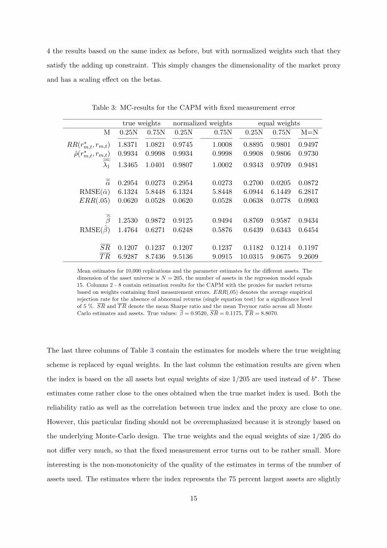
4 the results based on the same index as before, but with normalized weights such that they
satisfy the adding up constraint. This simply changes the dimensionality of the market proxy
and has a scaling effect on the betas.
Table 3: MC-results for the CAPM with fixed measurement error
true weights normalized weights equal weights
M 0.25N 0.75N 0.25N 0.75N 0.25N 0.75N M=N
RR(r∗m,t, rm,t) 1.8371 1.0821 0.9745 1.0008 0.8895 0.9801 0.9497
ρ(r∗m,t, rm,t) 0.9934 0.9998 0.9934 0.9998 0.9908 0.9806 0.9730
λ1 1.3465 1.0401 0.9807 1.0002 0.9343 0.9709 0.9481
α 0.2954 0.0273 0.2954 0.0273 0.2700 0.0205 0.0872RMSE(α) 6.1324 5.8448 6.1324 5.8448 6.0944 6.1449 6.2817ERR(.05) 0.0620 0.0528 0.0620 0.0528 0.0638 0.0778 0.0903
β 1.2530 0.9872 0.9125 0.9494 0.8769 0.9587 0.9434
RMSE(β) 1.4764 0.6271 0.6248 0.5876 0.6439 0.6343 0.6454
SR 0.1207 0.1237 0.1207 0.1237 0.1182 0.1214 0.1197
TR 6.9287 8.7436 9.5136 9.0915 10.0315 9.0675 9.2609
Mean estimates for 10,000 replications and the parameter estimates for the different assets. Thedimension of the asset universe is N = 205, the number of assets in the regression model equals15. Columns 2 - 8 contain estimation results for the CAPM with the proxies for market returnsbased on weights containing fixed measurement errors. ERR(.05) denotes the average empiricalrejection rate for the absence of abnormal returns (single equation test) for a significance levelof 5 %. SR and TR denote the mean Sharpe ratio and the mean Treynor ratio across all MonteCarlo estimates and assets. True values: β = 0.9520, SR = 0.1175, TR = 8.8070.
The last three columns of Table 3 contain the estimates for models where the true weighting
scheme is replaced by equal weights. In the last column the estimation results are given when
the index is based on the all assets but equal weights of size 1/205 are used instead of b∗. These
estimates come rather close to the ones obtained when the true market index is used. Both the
reliability ratio as well as the correlation between true index and the proxy are close to one.
However, this particular finding should not be overemphasized because it is strongly based on
the underlying Monte-Carlo design. The true weights and the equal weights of size 1/205 do
not differ very much, so that the fixed measurement error turns out to be rather small. More
interesting is the non-monotonicity of the quality of the estimates in terms of the number of
assets used. The estimates where the index represents the 75 percent largest assets are slightly
15

superior compared to the two other scenarios. If the index represents only the capitalization of
25 percent largest assets the estimates reveal the largest biases. For all scenarios we find a slight
over-rejection of the null of no abnormal returns.
3.2 Effects on Performance Measures
CAPM parameter estimates are frequently used to compute performance measures for single
assets or portfolios. Obviously the bias in the parameter estimates directly passes on to biases
in these performance measures. Consider, for instance, the Sharpe ratio and the Treynor ratio
for asset j = 1, . . . , N :
SRj =E [rj ]
σj=βj E [rm]
σjand TRj =
E [rj ]
βj= E [rm] .
In last two rows of Table 2 and Table 3 we report the estimates of average Sharpe ratios and
Treynor ratios under the different regimes of misspecification. The attenuation bias for beta also
leads to an attenuation bias for the Sharpe ratio, while for the Treynor ratio the attenuation bias
leads to a strong upward bias because the too small estimates for beta enter the denominator of
the Treynor ratio.
Figure 1 depicts the box plots for the estimated Treynor ratio for each of the 15 selected
assets. As implied by the theory the mean estimates are the same for all 15 assets and are equal
to the true value of the expected excess return of the market indicated by the blue horizontal
line. Note that due to the large sampling variation the Treynor ratio can only be estimated with
low precision, even in the absence of measurement error.
16

Figure 1: Estimates of the Treynor Ratio for 15 assets based on r∗m,t
Figure 2 depicts the box plots for the Treynor ratio based on equal weights and weights with
random measurement error. With measurement error in the market return we find an even
stronger variation in the performance across assets although the CAPM holds true. The presence
of measurement error mimics investment opportunities where none exist.
Figure 2: Estimates of the Treynor Ratio in the case of known asset universe and equallyweighted market index (left) or with random measurement error with σν = 0.05 (right)
The consequences of measurement error in the market return for investment decisions based
on CAPM estimates can also be seen for the security market line (SML). Figure 3 depicts the
unbiased CAPM estimates based on true market return (green dots) and the biased estimates
based on equal weights (blue dots). If the market return is measured correctly the estimates are
scattered closely around the SML indicating no need for reshuffling the portfolio. However, with
measurement error the estimates indicate investment opportunities due the spurious abnormal
returns. Note, that the case depicted here is based on the true SLM, i.e its slope is given by
µ∗. Since in the case of random measurement errors, µ∗ = µ the sample mean of the excess
return rm,t can serve as an unbiased estimate for the slope of the SML. However, in all other
17

cases considered µ∗ 6= µ, and the mean excess return of the market proxy does not yield a
consistent estimate of the slope. In this case the CAPM estimates deviate systematically from
the true SML as can be seen from Figure 9 in Appendix A.3. The biased estimated SML and
the attenuated CAPM beta estimates mimic investment opportunities with assets lying above
and below the estimated SML.
Figure 3: Security Market Line and CAPM estimates with and without Measurement Error.Green dots: estimates based on true market return. Blue dots: estimates based on equal weights.
4 Empirical Evidence in the Presence of Measurement Error
In the following we present empirical evidence on the relevance of measurement error in market
returns using our cross-equation identification strategy presented in Section 2.2. We use minimum
distance estimation (see Appendix A.1 for details) to estimate and test for attenuation bias and
the presence of abnormal returns for various datasets and alternative measures of the market
index. The effect of different market proxies on the beta estimates provides insights into the
robustness of CAPM estimates and the quantitative relevance of the measurement error problem.
In the first stage we estimate a CAPM system of regression equations by the seemingly unrelated
regression (SUR) approach. We call this system of regression equations CAPM linear projection
model (CAPM-LP) as it basically imposes no structure on the parameters implied by theory and
can be taken as a pure statistical concept. Alternatively, one may regard this model as a general
18

one-factor model with measurement error and/or abnormal returns, since non-zero intercepts
as a consequence of measurement error and abnormal returns are not separately identifiable.
The CAPM-LP, however, parametrically nests the standard CAPM (no abnormal returns, no
measurement error, N true betas) and the CAPM with measurement error (CAPM-ME) (λ1 6= 1,
N true betas and intercepts resulting solely from the presence of measurement error).
In the second estimation stage we impose the parametric structure implied either by the
CAPM-ME or the standard CAPM. For all the second stage estimates we use the inverse of the
first-stage variance covariance estimates as an optimal weighting matrix, so that the distance
statistics at the minimum are asymptotically χ2-distributed (see Appendix A.1). Tests for nested
specifications can then be obtained by comparing the distance statistics of the restricted model
against the less restricted specification. Thus the difference in the distance statistics of the
CAPM-ME against the CAPM-LP is χ2(N−1)-distributed and tests whether the intercepts can
solely be explained by the intercepts of the CAPM-ME. This test therefore circumvents the
problem of identifying the true from spurious alphas.
Assuming the CAPM-ME holds and imposing in addition the absence of any measurement
error, λ1 = 1, yields the minimum distance statistics for the standard CAPM. The difference
between the two corresponding distance statistics yields a χ2(1)-distributed test for the null
hypothesis that the CAPM holds against the more general CAPM-ME.
Finally, the χ2(N)-distributed Wald test on the zero intercepts tests in the tradition of the
CAPM against any alternative which implies non-zero intercepts (CAPM-ME, abnormal returns,
CAPM-ME including abnormal returns).
Table 4 summarizes the minimum distance estimates for three data sets consisting of different
securities: (i) 25 Fama-French portfolios formed on size (market capitalization) and book-to-
market ratio4, (ii) a set of 20 randomly selected stocks from the S&P 500 (iii) 30 stocks of
the Dow-Jones Industrial Average Index (DJIA). Our estimates are based on monthly data
of size T = 60 and three different definitions of the market return. As market index we use
the value-weighted return of all CRSP firms incorporated in the US and listed on the NYSE,
AMEX, or NASDAQ as provided on Kenneth French’s website, the S&P 500 value weighted
index and the Dow-Jones Industrial Average Index (DJIA). By construction the CRSP index is
the broadest index in terms of the asset space covered, while the DJIA is the crudest proxy of
4see http://mba.tuck.dartmouth.edu/pages/faculty/ken.french/data_library.html
19

the true market index. Therefore we would expect the lowest linear projection coefficient for the
DJIA and the strongest attenuation bias for the beta estimates.
Table 4: Minimum Distance Estimates and Tests under Measurement Error
French Fama S&P500 stocks DJ stocks
Market Index CRSP S&P500 DJIA CRSP S&P500 DJIA CRSP
CAPM vs. 61.98 32.72 38.28 28.18 61.88 100.47 30.94CAPM-LP (0.00) (0.04) (0.01) (0.11) (0.00) (0.00) (0.42)
CAPM-ME vs 39.16 26.23 26.12 26.95 32.03 31.99 30.90CAPM-LP (0.03) (0.12) (0.13) (0.11) (0.32) (0.32) (0.87)
CAPM vs 22.82 6.5 12.16 1.24 29.85 68.49 0.043CAPM-ME (0.00) (0.01) (0.00) (0.27) (0.00) (0.00) (0.84)
λ1 0.97 0.690 0.579 1.25 0.65 0.55 1.023
N 25 20 20 20 30 30 30T 60 60 60 60 60 60 60
Minimum distance estimates of the linear projection parameter λ1 and MD-based tests fordifferent data sets and measures of the market proxies, p-values in brackets. N denotes herethe number of assets in the regression model. Sampling period: 2010:06-2015:05 for all datasets.
Consider first the results of Wald test for the absence of intercepts (CAPM vs CAPM-LP).
Our findings are in accordance with many previous empirical studies rejecting the null of no
intercepts. However, note that in the presence of measurement error this test provides no
information whether the non-zero intercepts result from true abnormal returns or are spurious
due to measurement error. More interesting are the outcomes tor our test of the CAPM-ME
against the CAPM-LP. Except for the FF-data we find that the measurement specification is
sufficient to explain the presence of intercepts. Our test results indicate that the rejection of no
abnormal returns often found for many data sets are likely to be the outcome of measurement
error.
Note, that the linear projection coefficient λ1 can only be interpreted as reliability ratio in
the case of the EIV model. Only for this case the projection coefficient is bounded between by
construction zero and one and implies an attenuation bias in the betas. Using the S&P500 and
the DJIA as market proxies we find for all datasets significant evidence for an attenuation bias.
The situation for the CRSP index as market proxy is somewhat different: The null of λ1 = 1 for
20

the Dow-Jones and the S&P500 stocks cannot be rejected, while it has to be rejected for the FF
data. But for this case the attenuation bias is rather small.
5 Conclusions
In this paper we take a closer look at the consequences of a misspecified market index in the
capital asset pricing model. Our focus is on two major sources of misspecification: (i) the use of
inaccurate weights and (ii) the use of only a subset of the asset universe to construct the index.
The consequences resulting from the use of badly chosen market proxy reach from inconsistent
parameter estimates to a misinterpretation of tests on the existence of abnormal returns. High
correlations between market proxies and the true market return are shown to be an insufficient
to indicate that the choice of a particular market proxy is negligible. What matters is the
predictive quality of the market proxy for the true market index in terms of a linear projection.
The estimation problems arising from measurement error in the market proxy deviate
substantially from the ones typically found in errors-in-variable models for linear regressions.
Unlike the true market index, market proxies are no longer orthogonal to the error in the CAPM.
Instrumental variable estimation generally becomes infeasible, unless additional identifying
assumptions are introduced.
For the the EIV-CAPM model, where the errors in the weights of the market index are
assumed to be random, we present a new identification strategy. This strategy accounts for
nonlinear cross-equation identifying restrictions which exploit the property that all CAPM
equations are effected by the same attenuation bias for beta. Our estimation strategy allows
us to test the linear projection based asset pricing model incorporating abnormal returns and
measurement error against the EIV-CAPM as well as to test the CAPM with measurement error
against the conventional Sharpe-Lintner CAPM without abnormal returns and measurement
error. Our empirical findings indicate for three different datasets and different market proxies,
that regardless of the assets under investigation the use of a more accurate proxy is rewarding
and reduces the estimation bias. Moreover, our estimates indicate that the existence of abnormal
returns in the conventional CAPM is spurious and can largely be explained by measurement
error. In this sense Roll’s (1977) fundamental critique can somewhat be mitigated.
However, the claim of this study is a rather moderate one. We do not intend to give an
21

answer to the ongoing question of whether the CAPM is dead or alive. Our study simply points
out that if we want the CAPM to give a chance to survive as a workhorse in academic finance
and business, we should take it more seriously and try to account for the latency of the market
return as best as possible. In particular, this includes taking on a more skeptical view on the
evidence for the existence of abnormal returns in the presence of measurement error. Future
research should consider other types of measurement error (e.g. multiplicative errors) as well
as the consequences of measurement error in other multi-factor asset pricing models. In the
light of our findings it seems also rewarding to reconsider the construction of popular market
proxies which generally are characterized by a local bias contradicting the assumption that a
large fraction of the investors follow a global investment strategy and ignore returns from other
important tangible or non-tangible assets.
References
Campbell, J. Y., A. W. Lo, and A. C. MacKinlay (1997): The Econometrics of Financial
Markets, Princeton University Press.
Fama, E. F. and K. R. French (2004): “The Capital Asset Pricing Model: Theory and
Evidence,” Journal of Economic Perspectives, 18, 25–46.
Fan, J. and Q. Yao (2017): The Elements of Financial Econometrics, Cambridge: Cambridge
University Press.
Fuller, W. (1987): Measurement Error Models, Wiley.
Gibbons, M. R., S. A. Ross, and J. Shanken (1989): “A Test of the Efficiency of a Given
Portfolio,” Econometrica, 57, 1121–1152.
Gourieroux, C. and J. Jasiak (2001): Financial Econometrics, Princeton: Princeton
University Press.
Jaganathan, R., G. Skoulakis, and Z. Wang (2010): “The Analysis of the Cross-Section
of Security Returns,” in Handbook of Financial Econometrics, ed. by Y. Aıt-Sahalia and L. P.
Hansen, vol. Vol 2. - Applications, chap. 14.
Jagannathan, R. and Z. Wang (1996): “The Conditional CAPM and the Cross-Section of
Expected Returns,” Journal of Finance, 51, 3–53.
22

Kandel, S. and R. F. Stambaugh (1987): “On correlations and inferences about mean-
variance efficiency,” Journal of Financial Economics, 18, 61 – 90.
Lintner, J. (1965): “The Valuation of Risk Assets and the Selection of Risky Investments in
Stock Portfolios and Capitals Budgets,” Review of Economics and Statistics, 47, 13–73.
Prono, T. (2015): “Market proxies as factors in linear asset pricing models: Still living with
the roll critique,” Journal of Empirical Finance, 31, 36 – 53.
Roll, R. (1977): “A critique of the asset pricing theory’s tests Part I: On past and potential
testability of the theory,” Journal of Financial Economics, 4, 129–176.
Shanken, J. (1987): “Multivariate proxies and asset pricing relations : Living with the Roll
critique,” Journal of Financial Economics, 18, 91 – 110.
Sharpe, W. F. (1964): “Capital Asset Prices: A Theory of Market Equilibrium under Conditions
of Risk,” Journal of Finance, 19, 425–442.
Stambaugh, R. F. (1982): “On the exclusion of assets from tests of the two-parameter model:
A sensitivity analysis,” Journal of Financial Economics, 10, 237–268.
23

A Appendix
A.1 Minimum Distance Estimation of the CAPM
Consider the stochastic form of the linear predictor equation for the j-th excess return on the
(observable) excess return of the market rm,t including an intercept:
rj,t = X ′t πj + uj,t+1, j = 1, . . . , N,
where πj = (πj,1, πj,2)′ contains the reduced form parameters of a CAPM with measurement
error and X ′t = (1, rm,t). The collection of reduced form parameters into the so-called Π-matrix
of dimension N × 2 is given by
Π =
π′1
π′2...
π′N
=
µm(1− λ1)β1 λ1β1
µm(1− λ1)β2 λ1β2
......
µm(1− λ1)βN λ1βN
.
With Yt = rt = (rt1, rt2, . . . , rtN )′ as the vector of excess returns system of CAPM reduced for
regressions is given by
Yt = ΠXt + ut,
where Π = E[YtX′t]−1E[XtX
′t]−1 is the matrix of linear predictor coefficients with its sample
counterpart
Π =
(T∑t=1
YtX′t
)(T∑t=1
XtX′t
)−1
.
24

The Pi-matrix stacked into a row vector
π ≡ vec(Π′) = g(θ) =
µm(1− λ1)β1
λ1β1
µm(1− λ1)β2
λ1β2
...
µm(1− λ1)βN
λ1βN
relates the 2N -vector of reduced form parameters to a vector g(·) of nonlinear functions of
the structural parameter vector θ = (β′, λ1) of the same dimension, where π can be estimated
consistently by single equation least squares without loss of efficiency:
π = vec(
Π′)
=
π1
π2
...
πN
=
(X ′X)−1X ′Y1
(X ′X)−1X ′Y2
...
(X ′X)−1X ′YN
.
Under standard assumptions about the return process
√T (π − π)
d−→ N (0,Ω)
In the case of a homoskedastic error term vector with covariance matrix V [ut] = Σ, the
asymptotic variance-covariance matrix of π takes the well-known form
Ω = V [π] = Σ⊗ E[XtX
′t
]−1
assumed for seemingly unrelated regression models. Generalizations of Ω for the case of het-
eroskedasticity and autocorrelation can be easily derived.
25

The minimum distance estimator θ based on the restriction π = g(θ) is defined by
θ(WT ) = arg minθ∈Θ
[π − g(θ)]′WT [π − g(θ)],
where WT converges asymptotically to the positive definite matrix weighting matrix W0. The
optimal feasible weighting is given by WT = [ 1T Ω]−1, where Ω is a consistent estimate of the
asymptotic variance covariance matrix of π. Note, that g(·) depends on the unknown parameter
µm. In our empirical application, we replace µm by its sample mean.
26

A.2 Detailed Monte Carlo Results
27

Tab
le5:
MC
-res
ult
sfo
rth
eC
AP
Mw
ith
mea
sure
men
ter
ror
12
34
56
78
910
11
12
13
14
15
Mean
CAPM
r∗ m,t
α0.0
08
0.0
01
-0.0
07
-0.0
05
0.0
08
0.0
07
-0.0
08
0.0
06
-0.0
30
0.0
10
-0.0
14
-0.0
03
-0.0
18
-0.0
28
-0.0
18
-0.0
06
ERR
(.05)
0.0
55
0.0
51
0.0
51
0.0
52
0.0
51
0.0
47
0.0
52
0.0
48
0.0
50
0.0
51
0.0
54
0.0
49
0.0
53
0.0
57
0.0
51
0.0
51
β0.6
59
0.7
56
0.6
51
1.3
10
1.0
92
1.3
09
0.5
32
0.8
78
1.0
30
0.5
70
1.1
00
0.5
08
1.4
97
0.9
43
1.4
52
0.9
53
SR
0.2
12
0.1
92
0.1
76
0.1
51
0.0
78
0.0
67
0.1
24
0.1
45
0.0
81
0.1
04
0.0
70
0.1
26
0.0
99
0.1
36
0.0
90
0.1
23
TR
8.9
75
8.9
47
8.9
95
8.8
85
9.1
27
9.1
07
9.2
44
8.9
86
9.0
91
9.3
49
9.1
59
9.2
52
8.9
34
8.9
52
8.9
61
9.0
64
CAPM-EIVσν
=0.0
5
α3.5
48
4.1
36
3.5
32
6.9
81
5.8
74
6.8
77
2.8
21
4.6
32
5.3
16
3.0
30
5.6
88
2.6
84
7.8
27
4.9
26
7.5
02
5.0
25
ERR
(.05)
0.8
87
0.9
13
0.8
70
0.9
33
0.7
95
0.7
71
0.7
27
0.8
47
0.7
54
0.7
13
0.7
37
0.7
15
0.8
56
0.8
41
0.8
26
0.8
12
β0.2
07
0.2
43
0.2
05
0.3
98
0.3
38
0.3
88
0.1
59
0.2
59
0.2
94
0.1
69
0.3
20
0.1
49
0.4
32
0.2
78
0.4
12
0.2
83
SR
0.0
83
0.0
73
0.0
67
0.0
60
0.0
31
0.0
27
0.0
49
0.0
58
0.0
34
0.0
42
0.0
29
0.0
51
0.0
40
0.0
55
0.0
37
0.0
49
TR
14.6
87
-1.3
94
31.9
59
28.9
04
27.0
24
20.9
87
-9.7
51
13.2
05
-27.4
71
182.7
55
0.6
65
9.4
69
15.9
64
20.4
01
1.5
28
21.9
29
σν
=0.0
25
α1.8
32
2.0
99
1.8
09
3.6
59
3.0
51
3.6
65
1.4
88
2.4
72
2.8
73
1.6
11
3.0
54
1.4
35
4.2
13
2.6
13
4.0
80
2.6
64
ERR
(.05)
0.5
49
0.5
78
0.4
94
0.6
72
0.4
16
0.4
26
0.3
73
0.5
22
0.4
12
0.3
48
0.3
92
0.3
72
0.5
53
0.5
12
0.5
15
0.4
76
β0.4
72
0.5
50
0.4
68
0.9
20
0.7
77
0.9
04
0.3
70
0.6
05
0.6
96
0.3
95
0.7
49
0.3
49
1.0
18
0.6
50
0.9
76
0.6
60
SR
0.1
46
0.1
32
0.1
20
0.1
04
0.0
54
0.0
46
0.0
85
0.0
99
0.0
56
0.0
71
0.0
48
0.0
86
0.0
68
0.0
93
0.0
62
0.0
85
TR
13.4
35
12.9
68
12.6
12
9.3
76
11.9
97
15.3
65
20.6
78
8.4
71
14.5
18
4.6
85
13.3
62
10.5
00
14.8
90
13.6
27
11.7
34
12.5
48
σν
=0.0
1
α0.3
39
0.3
78
0.3
24
0.6
83
0.5
70
0.7
03
0.2
77
0.4
78
0.5
35
0.3
16
0.5
78
0.2
75
0.8
12
0.4
78
0.7
90
0.5
02
ERR
(.05)
0.0
87
0.0
78
0.0
67
0.0
98
0.0
72
0.0
74
0.0
75
0.0
77
0.0
71
0.0
66
0.0
77
0.0
76
0.0
99
0.0
83
0.0
95
0.0
80
β0.6
35
0.7
31
0.6
27
1.2
56
1.0
50
1.2
52
0.5
09
0.8
39
0.9
81
0.5
45
1.0
48
0.4
85
1.4
25
0.9
01
1.3
80
0.9
11
SR
0.2
01
0.1
82
0.1
66
0.1
43
0.0
74
0.0
63
0.1
17
0.1
37
0.0
77
0.0
98
0.0
66
0.1
19
0.0
93
0.1
28
0.0
85
0.1
17
TR
9.5
56
9.5
32
9.5
95
9.4
49
9.7
51
9.7
50
10.0
04
9.5
80
9.7
33
10.0
36
9.7
98
9.9
95
9.5
35
9.5
31
9.5
72
9.6
95
bI1
M=
0.2
5∗N
α-0
.059
-0.3
30
-0.1
77
0.0
31
-0.0
62
0.1
99
0.3
70
0.3
41
0.7
57
0.2
69
0.7
18
0.4
19
0.6
89
0.4
02
0.8
64
0.2
95
ERR
(.05)
0.0
56
0.0
67
0.0
55
0.0
50
0.0
53
0.0
51
0.0
66
0.0
63
0.0
71
0.0
60
0.0
64
0.0
72
0.0
69
0.0
63
0.0
73
0.0
62
β0.9
08
1.0
84
0.9
16
1.7
83
1.4
99
1.7
53
0.6
67
1.1
46
1.2
84
0.7
39
1.3
87
0.6
27
1.9
36
1.2
21
1.8
45
1.2
53
SR
0.2
16
0.2
02
0.1
82
0.1
52
0.0
79
0.0
66
0.1
14
0.1
39
0.0
75
0.0
99
0.0
65
0.1
14
0.0
95
0.1
29
0.0
84
0.1
21
TR
6.4
92
6.2
28
6.3
88
6.5
27
6.6
29
6.7
94
7.4
74
6.8
98
7.3
40
7.2
76
7.3
21
7.6
29
6.9
28
6.9
32
7.0
74
6.9
29
M=
0.7
5∗N
α-0
.015
-0.0
54
-0.0
45
-0.0
09
0.0
41
0.0
15
0.0
23
0.0
18
0.0
73
0.0
43
0.0
73
0.0
36
0.0
74
0.0
20
0.1
17
0.0
27
ERR
(.05)
0.0
56
0.0
53
0.0
51
0.0
50
0.0
53
0.0
51
0.0
52
0.0
52
0.0
55
0.0
54
0.0
52
0.0
54
0.0
52
0.0
56
0.0
52
0.0
53
β0.6
87
0.7
94
0.6
83
1.3
64
1.1
31
1.3
59
0.5
50
0.9
12
1.0
60
0.5
90
1.1
34
0.5
23
1.5
49
0.9
76
1.4
95
0.9
87
SR
0.2
14
0.1
94
0.1
78
0.1
52
0.0
78
0.0
67
0.1
24
0.1
45
0.0
81
0.1
03
0.0
70
0.1
25
0.0
99
0.1
36
0.0
90
0.1
24
TR
8.5
83
8.5
20
8.5
83
8.5
31
8.8
02
8.7
59
8.9
60
8.6
46
8.8
66
9.0
29
8.8
83
9.0
04
8.6
41
8.6
48
8.7
00
8.7
44
bI2
M=
0.2
5∗N
α-0
.059
-0.3
30
-0.1
77
0.0
31
-0.0
62
0.1
99
0.3
70
0.3
41
0.7
57
0.2
69
0.7
18
0.4
19
0.6
89
0.4
02
0.8
64
0.2
95
ERR
(.05)
0.0
56
0.0
67
0.0
55
0.0
50
0.0
53
0.0
51
0.0
66
0.0
63
0.0
71
0.0
60
0.0
64
0.0
72
0.0
69
0.0
63
0.0
73
0.0
62
β0.6
61
0.7
89
0.6
67
1.2
98
1.0
92
1.2
77
0.4
86
0.8
34
0.9
35
0.5
38
1.0
10
0.4
56
1.4
10
0.8
89
1.3
44
0.9
13
SR
0.2
16
0.2
02
0.1
82
0.1
52
0.0
79
0.0
66
0.1
14
0.1
39
0.0
75
0.0
99
0.0
65
0.1
14
0.0
95
0.1
29
0.0
84
0.1
21
TR
8.9
13
8.5
51
8.7
71
8.9
62
9.1
02
9.3
29
10.2
63
9.4
72
10.0
79
9.9
90
10.0
53
10.4
75
9.5
13
9.5
18
9.7
13
9.5
14
M=
0.7
5∗N
α-0
.015
-0.0
54
-0.0
45
-0.0
09
0.0
41
0.0
15
0.0
23
0.0
18
0.0
73
0.0
43
0.0
73
0.0
36
0.0
74
0.0
20
0.1
17
0.0
27
ERR
(.05)
0.0
56
0.0
53
0.0
51
0.0
50
0.0
53
0.0
51
0.0
52
0.0
52
0.0
55
0.0
54
0.0
52
0.0
54
0.0
52
0.0
56
0.0
52
0.0
53
β0.6
61
0.7
64
0.6
57
1.3
12
1.0
87
1.3
07
0.5
29
0.8
77
1.0
19
0.5
68
1.0
91
0.5
03
1.4
90
0.9
39
1.4
38
0.9
49
SR
0.2
14
0.1
94
0.1
78
0.1
52
0.0
78
0.0
67
0.1
24
0.1
45
0.0
81
0.1
03
0.0
70
0.1
25
0.0
99
0.1
36
0.0
90
0.1
24
TR
8.9
25
8.8
59
8.9
24
8.8
70
9.1
52
9.1
08
9.3
16
8.9
90
9.2
18
9.3
88
9.2
36
9.3
63
8.9
84
8.9
92
9.0
46
9.0
92
bI3
M=
0.2
5∗N
α0.3
05
0.3
20
0.2
18
0.2
18
1.0
16
-0.8
90
0.4
40
0.2
99
0.4
18
0.2
78
0.3
56
0.5
74
0.1
51
0.2
85
0.0
62
0.2
70
ERR
(.05)
0.0
71
0.0
65
0.0
57
0.0
55
0.0
83
0.0
70
0.0
70
0.0
61
0.0
60
0.0
58
0.0
54
0.0
88
0.0
55
0.0
59
0.0
52
0.0
64
β0.5
94
0.6
86
0.5
97
1.2
24
0.9
29
1.3
41
0.4
58
0.8
04
0.9
32
0.5
15
1.0
07
0.4
21
1.4
09
0.8
65
1.3
74
0.8
77
SR
0.2
02
0.1
83
0.1
70
0.1
49
0.0
70
0.0
72
0.1
13
0.1
39
0.0
78
0.0
99
0.0
68
0.1
10
0.0
99
0.1
31
0.0
90
0.1
18
TR
9.9
56
9.8
86
9.8
53
9.5
15
10.8
32
8.8
14
10.9
15
9.8
26
10.1
89
10.4
52
10.0
28
11.4
66
9.5
00
9.7
81
9.4
61
10.0
32
M=
0.7
5∗N
α0.5
04
1.0
05
0.6
07
0.6
64
1.1
43
-0.0
34
-0.3
51
-0.1
59
-0.7
41
-0.0
81
-0.5
02
-0.3
77
-0.3
53
-0.2
21
-0.7
95
0.0
21
ERR
(.05)
0.1
00
0.1
84
0.0
97
0.0
86
0.0
91
0.0
52
0.0
66
0.0
53
0.0
75
0.0
53
0.0
57
0.0
67
0.0
55
0.0
58
0.0
74
0.0
78
β0.6
07
0.6
49
0.5
88
1.2
47
0.9
71
1.3
24
0.5
76
0.9
05
1.1
22
0.5
87
1.1
66
0.5
55
1.5
52
0.9
75
1.5
55
0.9
59
SR
0.1
95
0.1
63
0.1
57
0.1
43
0.0
69
0.0
67
0.1
34
0.1
48
0.0
88
0.1
06
0.0
74
0.1
37
0.1
03
0.1
40
0.0
96
0.1
21
TR
9.7
56
10.5
19
10.0
43
9.3
48
10.3
76
8.9
70
8.4
36
8.6
89
8.2
82
9.0
97
8.5
66
8.3
64
8.6
03
8.6
39
8.3
24
9.0
68
M=N
α0.6
13
1.2
74
0.8
69
0.9
24
1.1
29
0.1
91
-0.2
54
-0.0
98
-0.9
31
-0.0
41
-0.5
81
-0.3
89
-0.3
01
-0.1
55
-0.9
41
0.0
87
ERR
(.05)
0.1
23
0.2
57
0.1
46
0.1
17
0.0
91
0.0
50
0.0
55
0.0
50
0.0
84
0.0
53
0.0
64
0.0
63
0.0
58
0.0
56
0.0
86
0.0
90
β0.5
91
0.6
13
0.5
52
1.2
07
0.9
67
1.2
90
0.5
61
0.8
91
1.1
34
0.5
77
1.1
66
0.5
53
1.5
31
0.9
59
1.5
59
0.9
43
SR
0.1
91
0.1
56
0.1
49
0.1
40
0.0
69
0.0
66
0.1
31
0.1
48
0.0
90
0.1
05
0.0
74
0.1
38
0.1
02
0.1
39
0.0
97
0.1
20
TR
10.0
52
11.1
77
10.7
20
9.6
68
10.4
36
9.2
32
8.6
78
8.8
34
8.1
74
9.1
85
8.5
68
8.3
89
8.7
13
8.7
82
8.3
04
9.2
61
Desc
ripti
on:
Avera
ge
resu
ltover
10000
replicati
ons.
Fir
stpanel
conta
ins
the
avera
ge
est
imate
sbase
don
the
true
(excess
)m
ark
et
retu
rn.
Furt
her
panels
conta
inest
imati
on
resu
lts
for
the
CA
PM
wit
hth
epro
xie
sof
the
mark
et
retu
rns
base
don
weig
hts
wit
hfi
xed
or
random
err
ors
.ERR
(.05)
denote
sth
eavera
ge
em
pir
ical
reje
cti
on
rate
for
the
abse
nce
of
abnorm
al
retu
rns
(sin
gle
equati
on
test
)fo
ra
signifi
cance
level
of
5%
.SR
andTR
denote
the
mean
Sharp
era
tio
and
the
mean
Tre
ynor
rati
oacro
ssall
Monte
Carl
oest
imate
s.T
rue
valu
es:β
=0.9
520,SR
=0.1
175,TR
=8.8
070.
28

A.3 Figures
(a) σν = 0.05
(b) σν = 0.025
(c) σν = 0.01
Figure 4: Sharpe Ratios of 15 assets based market indices with random measurement error
29

(a) 25%
(b) 75%
Figure 5: Sharpe Ratios of 15 assets based on market indices based on the subset of assets withtrue weights
30
(a) 25%
(b) 75%
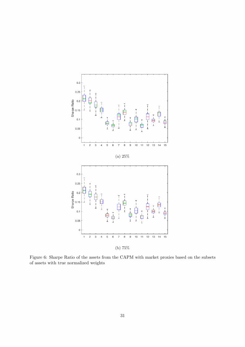
Figure 6: Sharpe Ratio of the assets from the CAPM with market proxies based on the subsetsof assets with true normalized weights
31

(a) 25%
(b) 75%
(c) 100%
Figure 7: Sharpe Ratio of the assets from the CAPM with market proxies based on the subsetsof assets with equal weights
32

Figure 8: Security Market Line and estimated betas in the case of random measurement error inthe weights of the market portfolio
33

(a) true weights for M stocks
(b) normalized true weights for M stocks
(c) equal weights for M stocks
Figure 9: Security Market Line and estimated betas in the case of misspecified index based onthe subset of assets
34