global climate models and their limitationsweather.missouri.edu/gcc/_09-09-13_ chapter 1...
TRANSCRIPT

9
1
Global Climate Models and Their Limitations Anthony Lupo (USA)
William Kininmonth (Australia) Contributing: J. Scott Armstrong (USA), Kesten Green (Australia)
1. Global Climate Models and Their Limitations Key Findings Introduction 1.1 Model Simulation and Forecasting 1.2 Modeling Techniques 1.3 Elements of Climate 1.4 Large Scale Phenomena and Teleconnections
Key Findings The IPCC places great confidence in the ability of general circulation models (GCMs) to simulate future climate and attribute observed climate change to anthropogenic emissions of greenhouse gases. They claim the “development of climate models has resulted in more realism in the representation of many quantities and aspects of the climate system,” adding, “it is extremely likely that human activities have caused more than half of the observed increase in global average surface temperature since the 1950s” (p. 9 and 10 of the Summary for Policy Makers, Second Order Draft of AR5, dated October 5, 2012).
This chapter begins with a brief review of the inner workings and limitations of climate models. Climate models are important tools utilized to advance our understanding of current and past climate. They also provide qualitative and quantitative information about potential future climate. But in spite of all their sophistication, they remain merely models. They represent simulations of the real world, constrained by their ability to correctly capture and portray each of the important processes that operate to affect climate. Notwithstanding their complexities, the models remain deficient in many aspects of their portrayal of the climate, which reduces their ability to provide reliable simulations of future climate.
Confidence in a model is further based on the careful evaluation of its performance, in which model output is compared against actual observations. A large portion of this chapter, therefore, is devoted to the evaluation of climate models against real-world climate and other biospheric data. That evaluation, summarized in the findings of numerous peer-reviewed scientific papers described in the different subsections of this chapter, reveals the IPCC is overestimating the ability of current state-of-the-art GCMs to accurately simulate both past and future climate. The IPCC’s stated confidence in the models, as presented at the beginning of this chapter, is likely exaggerated. The many and varied model deficiencies discussed in this chapter indicate much work remains to be done before model simulations can be treated with the level of confidence ascribed to them by the IPCC.
The following points summarize the main findings of this chapter: • Properties inherent in models make dynamic
predictability impossible. Without dynamic predictability, other techniques must be used to simulate climate. Such techniques introduce biases of varying magnitude into model projections.

Climate Change Reconsidered II
10
• To have any validity in terms of future projections, GCMs must incorporate not only the many physical processes involved in determining climate, but also all important chemical and biological processes that influence climate over long time periods. Several of these important processes are either missing or inadequately represented in today’s state-of-the-art climate models.
• Limitations in computing power frequently result in the inability of models to resolve important climate processes. Low-resolution models fail to capture many important phenomena of regional and lesser scales, such as clouds; downscaling to higher-resolution models introduces boundary interactions that can contaminate the modelling area and propagate error.
• The magnitude of the range of projected responses to a doubling of atmospheric CO2 by itself establishes that large errors and limitations in the models remain to be corrected.
• Many GCMs fail to account properly for certain “multiplier effects” that may significantly amplify the initial impacts of various biospheric processes. For example, although the absolute variations associated with some solar-related phenomena are rather small, Several multiplier effects may significantly amplify the initial perturbation.
• Major imperfections in the models prevent proper simulation of important elements of the climate system, including pressure, wind, clouds, temperature, precipitation, ocean currents, sea ice, permafrost, etc. Large differences between model predictions and observations frequently exist when comparing these elements or features. In some cases computer models fail to simulate even the correct sign of the observed parameters.
• Although some improvements have been noted in performance between the CMIP3 set of models used in AR4 and the newer CMIP5 models utilized in AR5, many researchers report finding little or no improvement in the CMIP5 model output for several important parameters and features of Earth’s climate.
Introduction Global Climate Models (GCMs) have evolved from the Atmospheric General Circulation Models (AGCMs) widely used for daily weather prediction. GCMs have been used for a range of applications, including investigating interactions between processes of the climate system, simulating evolution of the climate system, and providing projections of future climate states under scenarios that might alter the evolution of the climate system. The most widely recognized application is the projection of future climate states under various scenarios of increasing atmospheric carbon dioxide (CO2).
At the core of a GCM is an AGCM that dynamically simulates the circulation of the atmosphere, including the many processes that regulate energy transport and exchange by and within the atmospheric flow. The basic atmospheric flow is represented by fundamental equations that link the mass distribution and the wind field. These equations are represented on a spherically spatial grid field that has many levels representing the depth of the atmosphere. The flow equations are modified by the representation of processes that occur on a scale below that of the grid—including such processes as turbulence, latent heat of condensation in cloud formation, and dynamic heating as solar and infrared radiation interact with atmospheric gases, aerosols, and clouds.
The oceans are at least as important as the atmosphere for the transport of energy. For that reason, the GCM also includes an Ocean General Circulation Model (OGCM) that simulates the circulation of the oceans. The OGCM is vital for climate simulations because the oceans represent a dynamic thermal reservoir that, through energy exchange with the atmosphere, dominates the evolution of the climate system. The specification of the processes that regulate heat, moisture, and momentum exchanges between the ocean and atmosphere is crucial to the integrity of a GCM.
Land surface, and how soil moisture and vegetation type regulate heat, moisture, and momentum with the atmosphere, plays a lesser but nevertheless important role in the simulation of climate. Soil moisture and vegetation respond to local precipitation and affect the exchange of heat, moisture, and momentum with the atmosphere over time. The soil moisture and vegetation (and their regulation of land-atmosphere exchange processes) respond to the climate on the shorter time-scale of weather systems but, due to the varying accumulation
Global Climate Models and Their Limitations
11
of soil moisture, the influence of land surface on climate is on seasonal and interannual time-scales.
Surface ice sheets also have an important role in the evolution of the climate system. Their formation and expansion represent a lowering of the total energy of the climate system as a whole because latent heat is lost as water changes from the liquid to solid phase. Likewise, contraction of surface ice sheets represents an increase in the total energy of the climate system. The representation of heat, moisture, and momentum exchanges between ice surfaces and the atmosphere differs from that of land surfaces or ocean surfaces.
Dominating the climate system and its evolution are the radiation processes that regulate the input and output of energy. The shape of the rotating Earth, its distance from the Sun, and the characteristics of its orbit determine the nature of diurnal (daytime) and seasonal solar heating, including its maximum over the tropics. The shedding of energy by infrared radiation originates from the surface, from aerosols, from clouds, and from greenhouse gases of the atmosphere (CO2, H2O, O3, etc.). The latitudinal spread of infrared loss radiation is less than for solar radiation and results in excess solar radiation being absorbed over the tropics but excess radiation shedding over higher latitudes.
A primary function of the climate system is to transport energy from the tropics to higher latitudes; globally, there is an equilibrium between solar radiation absorption and infrared radiation loss to space. Of course, with such a complex system there is rarely perfect balance. At times, especially during the cycle of seasons, Earth is accumulating radiation energy and warming, whereas at other times it is losing energy and cooling. But the rate of radiation loss varies with temperature and acts as a natural thermostat: when Earth warms, the infrared radiation loss to space increases such that it exceeds the solar input and warming ceases; when Earth cools, the infrared radiation loss to space decreases such that solar radiation exceeds the infrared radiation loss and cooling ceases.
The natural thermostat is more complex than this simple portrayal because different components of the climate system interact with limited bands of the infrared radiation spectrum. In particular, variation in surface characteristics, boundary layer aerosol characteristics, cloud height and distribution, and concentration of individual greenhouse gases can all affect the local infrared radiation loss to space across characteristic wavelengths with none affecting the full spectrum. Variations in each component, while acting
on a limited wavelength band, will affect the local magnitude of infrared radiation loss to space. Apart from water vapor concentration these variations are not necessarily temperature-dependent. Thus a change to the internal structure of the climate system for whatever reason will—all else being equal—lead to change in Earth’s equilibrium temperature.
Within the AGCM there are many important processes that operate on scales below the resolution of the computational grid (sub-grid scale processes) and regulate local temperature, moisture, and momentum. Perhaps the most important of these is convection.
As described by Riehl and Malkus (1958), it is the “hot towers” of deep tropical convection that distribute the accumulating heat and latent energy of the tropical boundary layer through the troposphere. Correct specification of the mass flows within the cloud mass and its surroundings, including the updrafts and downdrafts, is essential for regulating the Hadley Cell circulation and the availability of tropical energy for transport to higher latitudes. Correct specification of the mass flows is also important if the local impact on temperature, water vapor, and momentum are to be quantified. Correctly specifying the mass flows remains a challenge to modelers.
In general, clouds and their interaction with the climate system are difficult to model. Clouds are an outcome of vertical motion and saturation, but the feedback to the circulation through radiation processes is sensitive. Although cloud fields tend to be regulated by the larger scale circulation, the processes leading to cloud formation and dissipation are operating on scales very much smaller than that of the computation grid, with individual clouds often occupying only a small part of a grid. Thus it is necessary for models to specify the climate interaction of a multitude of differing clouds across a grid space by a single process.
AGCMs are very complex and their output should be examined carefully and cautiously. In the physical sciences, mathematical models are often used to formalize a theory or hypothesis. For example, Newton’s famous law of gravity formalized a statement of how objects fall or attract each other under ideal conditions (without wind or friction, for example). Note that in Newton’s law “gravity” is undefined and remains undefined. Also, in this theory Newton was able to treat objects such as planets as point masses, a successful but auxiliary assumption. Textbook physics is largely made up of laws based on
Climate Change Reconsidered II
12
such idealized situations (point masses, frictionless planes, ideal geometric bodies), and in approx-imations to ideal situations the models of physics work extremely well.
In the real world, however, inhomogeneity and complexity make the basic laws of physics less reliable. Whereas the breakage of simple rods under strain is easy to model and predict, earthquakes, which are also a breakage problem but occur in a complex setting of heterogeneous rock, are not predictable. Just because laws of physics are used does not mean a process is predictable; the climate prediction problem is not “just physics” as some scientists like to claim. It is also helpful to remember the laws of physics were developed by many rounds of experimentation, but it is not possible to conduct experiments at the scale of the whole Earth.
This means models themselves are being tested, in any study using them, to examine the behavior of a phenomenon. The definition of an atmospheric (climate) model is: a hypothesis [frequently in the form of mathematical statements] that describes the processes physically important to describe the workings of the atmosphere (climate and/or climatic change), that has physical consistency in the model formulation, and the agreement with the observations that serve to ‘test’ the hypothesis [i.e., the model]. The model is typically approximated for testing the hypothesis, but the model should conform to reality (AMS Glossary, 2000).
Once formulated, any atmospheric or climate model is simply a “box” that represents our best estimate of the workings of the atmosphere or climate. It is our best guess or approximation of the main processes of the system being represented and the mechanisms that link the processes. These models can be as complex or as simple as the model creators make them.
A model can be statistical or dynamic, and here we focus mainly on dynamic models, or what are called general circulation models. In a dynamic model, the system is represented in three dimensions, the characteristics of the system are specified at an initial time, and the system is allowed to evolve with time in accordance with the governing equations and boundary conditions that link essential processes.
An Atmosphere-Ocean General Circulation Model (AOGCM) is composed of seven basic mathematical equations with seven basic variables that describe the instantaneous state of the atmosphere over time. This represents a closed and solvable set of equations that can describe atmospheric motions and
processes. The equations represent four basic physical principles; correct theories or models representing atmospheric motions will not violate these basic principles: (1) conservation of mass (dry mass and water mass), (2) conservation of energy, (3) conservation of momentum, and (4) elemental kinetic theory of gases. The equations are sequentially solved across the grid space for each time step such that the time directions of quantities at each grid point are affected by their neighbors according to the governing equations.
Physical processes for which there is no precise formulation, or where the formulation is on a scale below that able to be resolved in the model, are represented within these equations by parameterizations. Although generally based on observations and simple statistical relationships, the parameterizations often are no more than educated guesses. Representation of sub-grid scale processes is just one of the problems with models, but more computer programming resources are devoted to it than to the basic equations referred to above.
There are other problems with the models that manifest themselves as “computational error,” which with time will eventually cause the system evolution to depart from that of the prototype (e.g., Haltiner and Williams, 1980, Durran, 1999).
First, there simply are not enough data available to establish the initial conditions. For example, weather forecasts are made with data measured twice a day in the United States, but once a day in most other locations on the globe. Also, the highest density of weather information is garnered from stations over land, although data continue to be sparse over uninhabited regions. There are vast areas where the atmosphere is poorly represented or sampled by conventional land-based balloon soundings.
To some extent the data problem is overcome by the use of satellite information that has global coverage, albeit the satellite data differ somewhat from traditional thermometer-based observations. Atmospheric satellite sounding data differ from radiosonde data, and satellite-derived ocean skin temperature differs from ship and buoy observations of ocean surface temperature, to name just two. Differences between the satellite and traditional data need to be reconciled in the establishment of starting conditions and the evaluation of predictions.
Second, many atmospheric processes, such as thunderstorms, occur on space scales much smaller than a model’s resolution. Energy exchange processes occurring on scales below the resolution of the model
Global Climate Models and Their Limitations
13
must therefore be approximated, or parameterized at the larger scale, and are therefore no longer mechanistic.
The inability to make the required observations with infinite precision means there is always some degree of measurement error or uncertainty associated with the initial conditions at the commencement of the forecast period. This uncertainty and its impact on the flow evolution can be measured by using differential equations and then making multiple runs of the model with slight variations in initial conditions. The error associated with the initial conditions amplifies into the flow structure and propagates through the system with time where it can render a model’s prediction unreliable in as short a time as four days (e.g., Lorenz, 1965).
This is not to imply that increased resolution in the models will fix this problem. In fact, there is some indication that further increasing the resolution will lead to diminishing improvements when examined against the cost, in computer time and budgets, of increasing the resolution.
Third, there is also some difficulty in representing the mathematical processes of the basic equations on the fixed grid space. The resolution of the model means the processes cannot be adequately specified and errors in representing the local gradients are amplified during the forecast period. Numerical finite difference methods are used generally to solve the GCM equations. For some operations there are several types of methods available (e.g., Wicker and Skamarock, 2002), making numerical modeling a matter of choosing the right tool for the job.
GCMs have the added complexity of coupling an ocean model, with its own difficulties of process specification, to an atmospheric model and regulating the energy exchange processes through the system by specified energy constraints. As more processes are introduced into the climate model—such as the energetics of the cryosphere, water storage in soils, and the changing of vegetation patterns—the model becomes considerably more complex and the potential for errors to be generated and to amplify in the output is increased.
All of these problems must be balanced against the amount of data a computer can process and how long it takes to produce a model simulation. Thus even this brief discussion and introduction of computer models demonstrates the skepticism through which the validity of model simulations should be evaluated. Unfortunately, there is little discussion by the IPCC about these problems inherent
to the models. It also is critical to understand the difference
between weather forecasting and the generation of climate projections or scenarios. Weather forecasting, in principle, is referred to as an initial value problem. Observational data are gathered, quality-controlled, and rendered to the grid space. This is no small problem because data are gathered from several sources, must be checked for consistency with other data, and then are rendered to the grid space in a manner consistent with our basic understanding and assumptions about atmospheric structure and behavior. The forecasts that evolve from these initial conditions are then constrained by the governing equations. To be useful, the evolution of the atmospheric flow must faithfully render the movement, development, and decay of the weather systems specified in the initial analysis. For weather forecasting models it is the structure and movement of the synoptic scale weather systems that is important. It is not as important to maintain global energy equilibrium over the relatively short prediction period of weather forecast.
How far out in time a useful forecast can be generated depends on the size and rotation rate of a planet, as well as the mixture of gases that make up the atmosphere. Using Earth’s atmosphere and dimensions, it is widely accepted that a useful forecast can be made for no more than 10 to 15 days—referred to as the forecasting “wall.” Clearly, another strategy is needed in making both long-range weather and climate forecasts.
Climate modeling of the atmosphere also involves a boundary value problem. The climate system responds very quickly (relatively speaking) to changes in the pattern of radiation exchange to and from space and to changes in the pattern of heat and moisture exchange between the underlying surface and the atmosphere. Tectonic movements of the continents, on the other hand, are so slow that the land and ocean distribution is generally treated as a constant. But heat and moisture exchanges with the underlying surface vary significantly with ocean surface temperature distribution and vegetation states. Thus the concept of atmospheric climate can be thought of as a servant dependent on the underlying surface. To complicate matters, scientists are still not completely sure about how the exchange of heat and mass between the atmosphere and ocean (and land) take place.
The veracity of climate forecasts depends not only on the ability of the general circulation equations
Climate Change Reconsidered II
14
to reproduce the flow structures but also on the specification of the many sub-grid scale processes that regulate energy, moisture, and momentum exchanges at these scales. Errors in any of these specifications will bias local energy accumulations and become evident as a false trend in the evolution of local climate indices. Many of the sub-grid scale exchanges are functions of local temperature or temperature gradient; locally developing biases will propagate spatially with time.
Thus the main distinction between weather forecast models and climate models is that, in the former, the objective is to specify the individual weather systems and reproduce their travel and decay, together with the development of new systems, over time. For climate models the interest is not in individual weather systems that cannot be replicated beyond about two weeks, but in the subtle changes in energy reservoirs over time, especially warming land surfaces, the ocean surface mixed layer, and cryosphere extent. This difference in objective is very large in principle.
There are two distinct types of climate models. Diagnostic, or equilibrium climate models (ECMs) represent steady-state or unchanging processes with time. The ECM is most commonly solved for climatic means and variations and can employ statistical or dynamical methods, or some combination of these, to generate a future climate.
In the second type of climate model, the Prognostic, changes in variables with time are crucial. The time variation for a given variable is the desired output (i.e., a time series). Thus climatic means and variances are changing and can be calculated and compared over limited time intervals.
Both types of models are employed in the study of climate. Generally, the diagnostic model is simpler and produces numerical output faster. Prognostic models are more complex. Either modeling technique can be utilized to create future climate projections or scenarios.
One way of making a climate model projection is to start with today’s conditions in a weather forecast model retooled for climate simulation. Researchers “add” carbon dioxide to replicate the rise in greenhouse gases and then run the model to see what output it produces. This approach would seem to be ideal, except there are several atmosphere-ocean interaction processes acting on multiyear to multidecadal time scales that models have not yet mastered. Examples of these phenomena are the El Niño–Southern Oscillation (ENSO, or El Niño and La
Niña), the Arctic Oscillation (AO)/North Atlantic Oscillation (NAO), and, on longer time scales, the Pacific Decadal Oscillation (PDO) and Atlantic Multidecadal Oscillation (AMO). The physical workings of these processes are not yet well understood, thus it is not surprising there is difficulty in modeling them. The effect of these cycles on regional and even global climate is not trivial, and failure to understand a phenomenon does not excuse leaving it out of a model, which is often done. Omitting such phenomena subjects the models to additional errors and failure.
In evaluating model reliability, the standard assumption has been to compare model output with observations over a given period of Earth’s past climate, e.g. since 1850. Doing so, however, requires subjective adjustments to the model; for example, in order to replicate estimated changing solar intensity and atmospheric aerosol loading. These adjustments create additional sources of uncertainty, as limited data exist in the past and knowledge about internal variability and the role of multidecadal-to-century-scale climate cycles is also restricted.
Perhaps it is in light of such limitations that in Chapter 9 of the Intergovernmental Panel on Climate Change’s (IPCC) Fifth Assessment Report (AR5) (e.g., IPCC, 2013-I) it is conceded that “climate models provide realistic simulations of the large-scale features in the climate system and reproduce observed historical change with only some fidelity. The climate sensitivity of current models has not changed dramatically from that of models assessed in the AR4, in spite of many improvements to the models’ representation of physical processes.”
Another strategy in creating model projections is to first allow the climate model to equilibrate; i.e., to find a steady climate state under control conditions and then again under conditions that may exist in the future (e.g., double the CO2 concentration). Then, one can analyze the differences in equilibrium climates in order to project how the climate of this future time will look. It should be kept in mind that a steady-state climate may not exist in nature. What about projections that show global temperature may rise by as much as 1o C to 6o C by 2100 (e.g., IPCC, 2007-I)? Such projections are based on a strategy in which a model is run many, many times from a particular set of initial conditions followed by slightly altered initial conditions. This is called a model ensemble. Generally, due to many of the problems discussed here and to the nature of the basic equations used in the model, the large range in

Global Climate Models and Their Limitations
15
global temperature projections is a natural result of the ensemble technique. The more times a model is run and the longer the time period of evolution used, the greater the spread in the range of the predicted variable, such as global temperature. This is referred to as sensitivity to initial conditions (SDIC). Such behavior is inherent in any system that displays chaotic characteristics, as does Earth’s climate system. Chaos theory is another name for the study of such nonlinear dynamics, which are represented in the raw forms of the basic equations.
The IPCC places great confidence in the ability of GCMs to simulate future climate and attribute observed climate change to anthropogenic emissions of greenhouse gases. It says “climate models are based on well-established physical principles and have been demonstrated to reproduce observed features of recent climate … and past climate changes. … There is considerable confidence that Atmosphere-Ocean General Circulation Models (AOGCMs) provide credible quantitative estimates of future climate change, particularly at continental and larger scales” (IPCC, 2007-I, p. 591).
The IPCC’s confidence in the models, however, is likely considerably overstated. The magnitude of the range of projected temperature responses to a doubling of atmospheric CO2 itself suggests there are large errors and limitations in the models that must be overcome. To have any validity in terms of future projections, GCMs must incorporate not only the many physical processes described above but also the chemical and biological processes that influence climate over long time periods. In addition, current computational errors resulting from finite grid resolution must be overcome so as not to introduce growing biases. And as a final step, model output must be compared with and evaluated against real-world observations. The remainder of this chapter delves further into the complexities and problems inherent to computer modeling of the climate system. Other chapters in this volume serve to evaluate the model projections using real-world data observations. References American Meteorological Society (AMS). 2000. Glossary of Meteorology, Allen Press.
Durran, D.R. 1999. Numerical Methods for Wave Equations in Geophysical Fluid Dynamics. Springer-Verlag, Inc..
Haltiner, G.J. and Williams, R.T. 1980. Numerical Prediction and Dynamic Meteorology, 2nd ed. Wiley and Sons, Inc.
IPCC. 2013-I. Climate Change 2013: The Physical Science Basis. Contribution of Working Group I to the Fourth Assessment Report of the Intergovernmental Panel on Climate Change.
IPCC. 2007-I. Climate Change 2007: The Physical Science Basis. Contribution of Working Group I to the Fourth Assessment Report of the Intergovernmental Panel on Climate Change. Solomon, S., Qin, D. Manning, M. Chen, Z., Marquis, M. Averyt, K.B., Tignor, M., and Miller, H.L.. (Eds.) Cambridge University Press, Cambridge, UK.
Lorenz, E.N. 1965. A study of the predictability of a 28-variable model. Tellus 17: 321–333.
Riehl, H. and Malkus, J. 1958. On the heat balance in the equatorial trough zone. Geophysica 6: 3–4.
Wicker, L.J. and Skamarock, W.C. 2002. Time-splitting methods for elastic models using forward time schemes. Monthly Weather Review 130: 2088–2097.
1.1 Model Simulation and Forecasting 1.1.1 Methods and Principles J. Scott Armstrong, a professor at The Wharton School of the University of Pennsylvania and a leading figure in forecasting, has pointed out that forecasting is a scientific discipline built on more than 70 years of empirical research, with its own institute (International Institute of Forecasters, founded in 1981), peer-reviewed journals (International Journal of Forecasting and Journal of Forecasting), and annual International Symposium on Forecasting. The research on forecasting has been summarized as scientific principles, currently numbering 140, that must be observed in order to make valid and useful forecasts (Principles of Forecasting: A Handbook for Researchers and Practitioners, edited by J. Scott Armstrong, Kluwer Academic Publishers, 2001).
When physicists, biologists, and other scientists who are unaware of the rules of forecasting attempt to make climate predictions, their forecasts are at risk of being no more reliable than those made by non-experts, even when they are communicated through complex computer models (Green and Armstrong, 2007). In other words, when faced with forecasts by scientists, even large numbers of very distinguished scientists, one cannot assume the forecasts are scientific. Green and Armstrong cite research by Philip E. Tetlock (2005), a psychologist and now
Climate Change Reconsidered II
16
professor at the University of Pennsylvania, who “recruited 288 people whose professions included ‘commenting or offering advice on political and economic trends.’ He asked them to forecast the probability that various situations would or would not occur, picking areas (geographic and substantive) within and outside their areas of expertise. By 2003, he had accumulated more than 82,000 forecasts. The experts barely, if at all, outperformed non-experts, and neither group did well against simple rules” (Green and Armstrong, 2007). The failure of expert opinion to provide reliable forecasts has been confirmed in scores of empirical studies (Armstrong, 2006; Craig et al., 2002; Cerf and Navasky, 1998; Ascher, 1978) and illustrated in historical examples of wrong forecasts made by leading experts, including such luminaries as Ernest Rutherford and Albert Einstein (Cerf and Navasky, 1998).
In 2007, Armstrong and Kesten C. Green of the Ehrenberg-Bass Institute at the University of South Australia conducted a “forecasting audit” of the IPCC Fourth Assessment Report (Green and Armstrong, 2007). The authors’ search of the contribution of Working Group I to the IPCC “found no references … to the primary sources of information on forecasting methods” and “the forecasting procedures that were described [in sufficient detail to be evaluated] violated 72 principles. Many of the violations were, by themselves, critical.”
Green and Armstrong found the IPCC violated “Principle 1.3 Make sure forecasts are independent of politics.” The two authors write, “this principle refers to keeping the forecasting process separate from the planning process. The term ‘politics’ is used in the broad sense of the exercise of power.” Citing David Henderson (2007), a former head of economics and statistics at the Organization for Economic Cooperation and Development (OECD), Green and Armstrong state, “the IPCC process is directed by non-scientists who have policy objectives and who believe that anthropogenic global warming is real and dangerous.” They thus conclude:
The forecasts in the Report were not the outcome of scientific procedures. In effect, they were the opinions of scientists transformed by mathematics and obscured by complex writing. Research on forecasting has shown that experts’ predictions are not useful in situations involving uncertainty and complexity. We have been unable to identify any scientific forecasts of global warming. Claims that the Earth will get warmer have no more credence than saying that it will get colder.
Scientists working in fields characterized by complexity and uncertainty are apt to confuse the output of models—which are nothing more than a statement of how the modeler believes a part of the world works—with real-world trends and forecasts (Bryson, 1993). Computer climate modelers frequently fall into this trap and have been severely criticized for failing to notice their models fail to replicate real-world phenomena by many scientists, including Balling (2005), Christy (2005), Essex and McKitrick (2007), Frauenfeld (2005), Michaels (2000, 2005, 2009), Pilkey and Pilkey-Jarvis (2007), Posmentier and Soon (2005), and Spencer (2008).
Canadian science writer Lawrence Solomon (2008) asked many of the world’s leading scientists active in fields relevant to climate change for their views on the reliability of computer models used by the IPCC to detect and forecast global warming. Their answers showed a high level of skepticism:
• Prof. Freeman Dyson, professor of physics at the Institute for Advanced Study at Princeton University and one of the world’s most eminent physicists, said the models used to justify global warming alarmism are “full of fudge factors” and “do not begin to describe the real world.”
• Dr. Zbigniew Jaworowski, chairman of the Scientific Council of the Central Laboratory for Radiological Protection in Warsaw and former chair of the United Nations Scientific Committee on the Effects of Atomic Radiation, a world-renowned expert on the use of ancient ice cores for climate research, said the U.N. “based its global-warming hypothesis on arbitrary assumptions and these assumptions, it is now clear, are false.”
• Dr. Richard Lindzen, professor of meteorology at the Massachusetts Institute of Technology and member of the National Research Council Board on Atmospheric Sciences and Climate, said the IPCC is “trumpeting catastrophes that couldn’t happen even if the models were right.”
• Prof. Hendrik Tennekes, director of research at the Royal Netherlands Meteorological Institute, said “there exists no sound theoretical framework for climate predictability studies” used for global warming forecasts.
• Dr. Richard Tol, principal researcher at the Institute for Environmental Studies at Vrije Universiteit and adjunct professor at the Center for Integrated Study of the Human Dimensions of Global Change at Carnegie Mellon University, said the IPCC’s Fourth Assessment Report is “preposterous ...
Global Climate Models and Their Limitations
17
alarmist and incompetent.” • Dr. Antonino Zichichi, emeritus professor of
physics at the University of Bologna, former president of the European Physical Society, and one of the world’s foremost physicists, said global warming models are “incoherent and invalid.”
Princeton’s Freeman Dyson has written elsewhere, “I have studied the climate models and I know what they can do. The models solve the equations of fluid dynamics, and they do a very good job of describing the fluid motions of the atmosphere and the oceans. They do a very poor job of describing the clouds, the dust, the chemistry, and the biology of fields and farms and forests. They do not begin to describe the real world that we live in” (Dyson, 2007).
Many of the scientists cited above observe computer models can be “tweaked” to reconstruct climate histories after the fact. But this provides no assurance that the new model will do a better job of forecasting future climates, and it points to how unreliable the models are. Individual climate models often have widely differing assumptions about basic climate mechanisms but are then “tweaked” to produce similar forecasts. This is nothing like how real scientific forecasting is done.
Kevin Trenberth, a lead author along with Philip D. Jones of Chapter 3 of the Working Group I contribution to the IPCC’s Fourth Assessment Report, replied to some of these scathing criticisms on the blog of the science journal Nature. He argued “the IPCC does not make forecasts” but “instead proffers ‘what if’ projections of future climate that correspond to certain emissions scenarios” and then hopes these “projections” will “guide policy and decision makers” (Trenberth, 2007). He says “there are no such predictions [in the IPCC reports] although the projections given by the Intergovernmental Panel on Climate Change (IPCC) are often treated as such. The distinction is important.”
This defense is hardly satisfactory. As Green and Armstrong (2007) point out, “the word ‘forecast’ and its derivatives occurred 37 times, and ‘predict’ and its derivatives occurred 90 times in the body of Chapter 8 of the Working Group I report, and a survey of climate scientists conducted by those same authors found “most of our respondents (29 of whom were IPCC authors or reviewers) nominated the IPCC report as the most credible source of forecasts (not ‘scenarios’ or ‘projections’) of global average temperature.” Green and Armstrong conclude, “the IPCC does provide forecasts.”
Green and Armstrong subsequently collaborated with Willie Soon in conducting validation tests of the IPCC forecasts of global warming (Green, Armstrong, and Soon 2009). To do so, they tested whether the warming-trend forecasts used by the IPCC are more accurate than the standard benchmark forecast that there will be no change. They tested the IPCC’s “business as usual” 0.03˚C p.a. forecast and the no-change forecast from one to 100 years ahead on a rolling basis over the period of exponentially increasing human CO2 emissions from 1851 to 1975. The procedure generated 7,550 forecasts from each of the forecasting procedures.
The Green, Armstrong, and Soon validation test was a weak one, in that the IPCC forecasts were tested against historical data (HadCRUt3) the IPCC modelers knew exhibited a warming trend. Green, Armstrong, and Soon therefore were surprised to find the errors from the IPCC warming trend forecasts were nearly eight times greater than the errors from the no-change forecasts. For the longer 91 to 100 years-ahead forecast horizons, the IPCC errors were nearly 13 times greater for the 305 forecasts. The no-change forecasts were so accurate in the validation test that the authors forecast annual global mean temperatures will be within 0.5˚C of the 1988 figure for the next 100 years. For public policy and business planning purposes, it is hard to see that any economic benefit could be obtained from forecasts that were less accurate than forecasts from the no-change model. The implication of the Green, Armstrong, and Soon forecasts is that the best policy is to do nothing about global warming. Their findings did not, however, stop the claims that “we are at a turning point” and “it is different this time.”
If public policy to address global warming is to be made rationally, it must be based on scientific forecasts of (1) substantial global warming, the effects of which are (2) on balance seriously harmful, and for which (3) cost-effective policies can be implemented. Armstrong, Green, and Soon (2011) refer to these logical requirements of policymaking as “the 3-legged stool” of global warming policy. A failure of any leg would invalidate policies. To date, there are no evidence-based forecasts to support any of the legs. References Armstrong, J.S. 2001. Principles of Forecasting—A Handbook for Researchers and Practitioners. Kluwer Academic Publishers, Norwell, MA.
Climate Change Reconsidered II
18
Armstrong, J.S. 2006. Findings from evidence-based forecasting: Methods for reducing forecast error. International Journal of Forecasting 22: 583–598.
Armstrong, J.S., Green, K.C., and Soon, W. 2011. Research on forecasting for the global warming alarm. Energy and Environment 22: 1091–1104.
Ascher, W. 1978. Forecasting: An Appraisal for Policy Makers and Planners. Johns Hopkins University Press. Baltimore, MD.
Balling, R.C. 2005. Observational surface temperature records versus model predictions. In Michaels, P.J. (Ed.) Shattered Consensus: The True State of Global Warming. Rowman & Littlefield. Lanham, MD. 50–71.
Bryson, R.A. 1993. Environment, environmentalists, and global change: A skeptic’s evaluation. New Literary History 24: 783–795.
Cerf, C. and Navasky, V. 1998. The Experts Speak. Johns Hopkins University Press. Baltimore, MD.
Christy, J. 2005. Temperature changes in the bulk atmosphere: Beyond the IPCC. In Michaels, P.J. (Ed.) Shattered Consensus: The True State of Global Warming. Rowman & Littlefield. Lanham, MD. 72–105.
Craig, P.P., Gadgil, A., and Koomey, J.G. 2002. What can history teach us? A retrospective examination of long-term energy forecasts for the United States. Annual Review of Energy and the Environment 27: 83–118.
Dyson, F. 2007. Heretical thoughts about science and society. Edge: The Third Culture. August.
Essex, C. and McKitrick, R. 2007. Taken by Storm. The Troubled Science, Policy and Politics of Global Warming. Key Porter Books. Toronto, Canada.
Frauenfeld, O.W. 2005. Predictive skill of the El Niño-Southern Oscillation and related atmospheric teleconnections. In Michaels, P.J. (Ed.) Shattered Consensus: The True State of Global Warming. Rowman & Littlefield. Lanham, MD. 149–182.
Green, K.C. and Armstrong, J.S. 2007. Global warming: forecasts by scientists versus scientific forecasts. Energy Environ. 18: 997–1021.
Green, K.C., Armstrong, J.S., and Soon, W. 2009. Validity of climate change forecasting for public policy decision making. International Journal of Forecasting 25: 826–832.
Henderson, D. 2007. Governments and climate change issues: The case for rethinking. World Economics 8: 183–228.
Michaels, P.J. 2009. Climate of Extremes: Global Warming Science They Don’t Want You to Know. Cato Institute.
Washington, DC.
Michaels, P.J. 2005. Meltdown: The Predictable Distortion of Global Warming by Scientists, Politicians and the Media. Cato Institute, Washington, DC.
Michaels, P.J. 2000. Satanic Gases: Clearing the Air About Global Warming. Cato Institute. Washington, DC.
Pilkey, O.H. and Pilkey-Jarvis, L. 2007. Useless Arithmetic. Columbia University Press, New York, NY.
Posmentier, E.S. and Soon, W. 2005. Limitations of computer predictions of the effects of carbon dioxide on global temperature. In Michaels, P.J. (Ed.) Shattered Consensus: The True State of Global Warming. Rowman & Littlefield. Lanham, MD. 241–281.
Solomon, L. 2008. The Deniers: The World Renowned Scientists Who Stood Up Against Global Warming Hysteria, Political Persecution, and Fraud—And those who are too fearful to do so. Richard Vigilante Books. Minneapolis, MN.
Spencer, R. 2008. Climate Confusion: How Global Warming Hysteria Leads to Bad Science, Pandering Politicians and Misguided Policies that Hurt the Poor. Encounter Books, New York, NY.
Tetlock, P.E. 2005. Expert Political Judgment—How Good Is It? How Can We Know? Princeton University Press, Princeton, NJ.
Trenberth, K.E. 2007. Global warming and forecasts of climate change. Nature blog. http://blogs.nature.com/ climatefeedback/2007/07/global_warming_and_forecasts_o.html. Last accessed May 6, 2009.
1.1.2 Computational Issues To commemorate the publication of the 100th volume of the journal Climatic Change, Norman Rosenberg (Rosenberg, 2010) was asked to contribute an overview paper on progress that had occurred since the journal’s inception in the interrelated areas of climate change, agriculture, and water resources. Rosenberg accepted and at the age of 80 conducted his review quite admirably.
He began by noting the “overarching concern” of the volumes he edited was “to gain understanding of how climatic change affects agricultural production, unmanaged ecosystems and water resources; how farmers, foresters and water managers can strengthen these sectors against the negative impacts of climatic change and capitalize on positive impacts if any; how they can adapt to impacts that cannot be so modified or ameliorated and how they can contribute directly or indirectly to mitigation of anthropogenic climatic

Global Climate Models and Their Limitations
19
change—as, for example, through soil carbon sequestration and the production of biomass to substitute in part for the fossil fuels that are adding CO2 to the atmosphere.”
Rosenberg writes in his closing paragraph, “it seems difficult to say with assurance that the ‘state-of-the-art’ in projecting climatic change impacts on agriculture and water resources and unmanaged ecosystems is, today, that much better than it was 30 years ago,” noting “the uncertainty and lack of agreement in GCMs is still too great.” He reported, “much can and has been learned about possible outcomes,” but “for actual planning and policy purposes we are still unable to assure those who need to know that we can forecast where, when and how much agriculture (as well as unmanaged ecosystems and water resources) will be affected by climatic change.”
A similarly pessimistic commentary on the state of climate modeling appeared in 2010 in Nature Reports Climate Change. Kevin Trenberth, head of the Climate Analysis Section of the National Center for Atmospheric Research in Boulder, Colorado (USA), writes that one of the major objectives of upcoming climate modeling efforts will be to develop “new and better representations of important climate processes and their feedbacks.” The new work, Trenberth wrote, should increase “our understanding of factors we previously did not account for ... or even recognize.”
In expressing these sentiments, Rosenberg and Trenberth gave voice to the concerns of many scientists who are skeptical of the reliability of GCMs. Such concerns should not be misinterpreted as “denial.” Trenberth, at least, would deny being a “skeptic” of the theory of anthropogenic global warming. It is, rather, the humility of true scientists who—attempting to comprehend the complexity of the world of nature and its innermost workings—are well aware of their own limitations and those of all seekers of scientific truths. Although much has been learned, as Rosenberg and Trenberth outline in their respective essays, what is known pales in comparison to what is required “for actual planning and policy purposes,” as Rosenberg describes it, or “certainty” as Trenberth puts it.
In contrast, consider a paper that fails to recognize any such problems. Published in the Proceedings of the National Academy of Sciences of the United States of America and written by Susan Solomon (a co-chair of the IPCC’s 2007 Working Group 1 report for AR4) and three coauthors, it
claims to show “climate change that takes place due to increases in carbon dioxide concentration is largely irreversible for 1,000 years after emissions stop” (Solomon et al., 2009). In the virtual world of computer-run climate models, that may be the case, but that may not be true of the real world. Consider, for example, that the discernible climate signal from a major volcanic eruption is lost after only a few years.
In their paper, Solomon et al. set forth three criteria they say should be met by the modeled climatic parameters they studied: “(i) observed changes are already occurring and there is evidence for anthropogenic contributions to these changes, (ii) the phenomen[a] [are] based upon physical principles thought to be well understood, and (iii) projections are available and are broadly robust across models.”
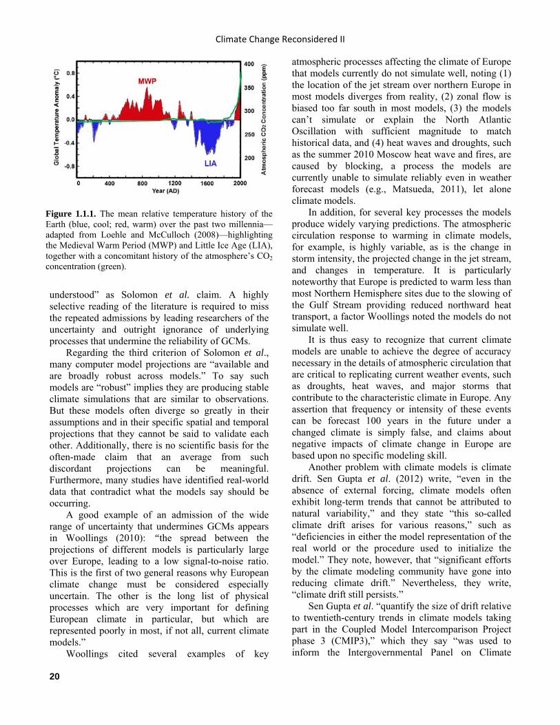
Real-world data provide little or no support for the first criterion (as discussed in other chapters of this volume). The global warming of the past few decades was part of a much longer warming trend that began in many places throughout the world a little more than three centuries ago (about 1680) with the dramatic “beginning of the end” of the Little Ice Age (LIA, see Figure 1.1.1), well before there was any significant increase in the air’s CO2 content. This observation suggests a continuation of whatever phenomenon—or combination of phenomena—may have caused the greater initial warming may have caused the lesser final warming, the total effect of which has been to transport Earth from the chilly depths of the Little Ice Age into the relative balminess of the Current Warm Period.
Climate history is discussed in greater detail in Chapter 4, but it is useful to note here that Earth’s current temperature is no higher now (and may be slightly less) than it was during the peak warmth of the Medieval Warm Period (MWP), when there was more than 100 ppm less CO2 in the air atmosphere there is today. Consequently, since the great MWP-to-LIA cooling phase occurred without any significant change in the atmosphere’s CO2 concentration, the opposite could occur just as easily. The planet could warm, and by an equal amount, just as it actually did over the past three centuries without any help from an increase in the atmosphere’s CO2 content.
Regarding the second criterion of Solomon et al., studies reported in this volume (see Chapter 2) also show there are non-modeled chemical and biological processes that may be equally as important as the changes in radiation fluxes associated with carbon dioxide employed in the models. The chemical and biological processes are simply not as “well
Climate Change Reconsidered II
20
understood” as Solomon et al. claim. A highly selective reading of the literature is required to miss the repeated admissions by leading researchers of the uncertainty and outright ignorance of underlying processes that undermine the reliability of GCMs.
Regarding the third criterion of Solomon et al., many computer model projections are “available and are broadly robust across models.” To say such models are “robust” implies they are producing stable climate simulations that are similar to observations. But these models often diverge so greatly in their assumptions and in their specific spatial and temporal projections that they cannot be said to validate each other. Additionally, there is no scientific basis for the often-made claim that an average from such discordant projections can be meaningful. Furthermore, many studies have identified real-world data that contradict what the models say should be occurring.
A good example of an admission of the wide range of uncertainty that undermines GCMs appears in Woollings (2010): “the spread between the projections of different models is particularly large over Europe, leading to a low signal-to-noise ratio. This is the first of two general reasons why European climate change must be considered especially uncertain. The other is the long list of physical processes which are very important for defining European climate in particular, but which are represented poorly in most, if not all, current climate models.”
Woollings cited several examples of key
atmospheric processes affecting the climate of Europe that models currently do not simulate well, noting (1) the location of the jet stream over northern Europe in most models diverges from reality, (2) zonal flow is biased too far south in most models, (3) the models can’t simulate or explain the North Atlantic Oscillation with sufficient magnitude to match historical data, and (4) heat waves and droughts, such as the summer 2010 Moscow heat wave and fires, are caused by blocking, a process the models are currently unable to simulate reliably even in weather forecast models (e.g., Matsueda, 2011), let alone climate models.
In addition, for several key processes the models produce widely varying predictions. The atmospheric circulation response to warming in climate models, for example, is highly variable, as is the change in storm intensity, the projected change in the jet stream, and changes in temperature. It is particularly noteworthy that Europe is predicted to warm less than most Northern Hemisphere sites due to the slowing of the Gulf Stream providing reduced northward heat transport, a factor Woollings noted the models do not simulate well.
It is thus easy to recognize that current climate models are unable to achieve the degree of accuracy necessary in the details of atmospheric circulation that are critical to replicating current weather events, such as droughts, heat waves, and major storms that contribute to the characteristic climate in Europe. Any assertion that frequency or intensity of these events can be forecast 100 years in the future under a changed climate is simply false, and claims about negative impacts of climate change in Europe are based upon no specific modeling skill.
Another problem with climate models is climate drift. Sen Gupta et al. (2012) write, “even in the absence of external forcing, climate models often exhibit long-term trends that cannot be attributed to natural variability,” and they state “this so-called climate drift arises for various reasons,” such as “deficiencies in either the model representation of the real world or the procedure used to initialize the model.” They note, however, that “significant efforts by the climate modeling community have gone into reducing climate drift.” Nevertheless, they write, “climate drift still persists.”
Sen Gupta et al. “quantify the size of drift relative to twentieth-century trends in climate models taking part in the Coupled Model Intercomparison Project phase 3 (CMIP3),” which they say “was used to inform the Intergovernmental Panel on Climate
Figure 1.1.1. The mean relative temperature history of the Earth (blue, cool; red, warm) over the past two millennia—adapted from Loehle and McCulloch (2008)—highlighting the Medieval Warm Period (MWP) and Little Ice Age (LIA), together with a concomitant history of the atmosphere’s CO2 concentration (green).
Global Climate Models and Their Limitations
21
Change (IPCC) Forth Assessment Report (AR4).” According to the seven Australian scientists, their
analysis determined that below 1-2 km in the deep ocean, or for depth-integrated properties, drift generally dominates over any forced trend. They report drift in sea level can be large enough to reverse the sign of the forced change, “both regionally and in some models for the global average.” In addition, because surface drift is spatially heterogeneous, they say “the regional importance of drift for individual models can be much larger than the global figures suggest.” As an example, they note “a typical error in calculating a regional forced sea surface temperature trend in the Bjerknes Center for Climate Research Bergen Climate Model, version 2.0 (BCM2.0), CSIRO Mk3.0, and GISS-EH models without accounting for drift would be 30% to 40%.” Because this is an average value, still-larger errors would be expected at some locations.
While providing some suggestions for addressing climate drift modeling problems, Sen Gupta et al. write, “in the absence of a clear direction forward to alleviate climate drift in the near term, it seems important to keep open the question of flux adjustment within climate models that suffer from considerable drift.” They indicate “flux adjustments are nonphysical and therefore inherently undesirable” and “may also fundamentally alter the evolution of a transient climate response,” citing the work of Neelin and Dijkstra (1995) and Tziperman (2000).
References Idso, S.B. 1998. CO2-induced global warming: A skeptic’s view of potential climate change. Climate Research 10: 69–82.
Loehle, C. and McCulloch, J.H. 2008. Correction to: A 2000-year global temperature reconstruction based on non-tree ring proxies. Energy & Environment 19: 93–100.
Matsueda, M. 2011. Predictability of Euro-Russian blocking in summer of 2010. Geophysical Research Letters 38: L06801, doi:10.1029/2010GL046557.
Neelin, J.D. and Dijkstra, H.A. 1995. Ocean-atmosphere interaction and the tropical climatology. Part I: The dangers of flux correction. Journal of Climate 8: 1325–1342.
Rosenberg, N.J. 2010. Climate change, agriculture, water resources: What do we tell those that need to know? Climatic Change 100: 113–117.
Sen Gupta, A., Muir, L.C., Brown, J.N., Phipps, S.J., Durack, P.J., Monselesan, D., and Wijffels, S.E. 2012.
Climate drift in the CMIP3 models. Journal of Climate 25: 4621–4640.
Solomon, S., Plattner, G.-K., Knutti, R., and Friedlingstein, P. 2009. Irreversible climate change due to carbon dioxide emissions. Proceedings of the National Academy of Sciences USA 106: 1704–1709.
Trenberth, K. 2010. More knowledge, less certainty. Nature Reports Climate Change: 10.1038/climate.2010.06.
Tziperman, E. 2000. Uncertainties in thermohaline circulation response to greenhouse warming. Geophysical Research Letters 27: 3077–3080.
Woollings, T. 2010. Dynamical influences on European climate: An uncertain future. Philosophical Transactions of the Royal Society A 368: 3733–3756.
1.1.3 Dealing with Chaos 1.1.3.1 Chaotic Systems The ability of atmosphere-ocean GCMs to predict the climatic effects of human alterations of greenhouse gases and other factors cannot be tested directly with respect to a point in time a hundred years in the future. However, it is still possible to determine whether those models can in principle make such predictions with a reasonable degree of accuracy.
One way to evaluate this ability is to consider the effects of errors in system initial values. If a system is well-behaved, small initial errors will lead to small future errors or even damped responses. In a chaotic system, on the other hand, small initial errors will cause trajectories to diverge over time; for such a system (or model), true predictability is low to nonexistent. This does not mean realistic behavior in the statistical sense cannot be simulated, only that detailed predictability (will it rain 60 days from now, or how much will it rain this year) is impossible. 1.1.3.2 Sensitivity Dependence One of the characteristics of chaotic systems, such as the fluid we call our atmosphere, is sensitive dependence on the initial conditions (SDIC). SDIC means one can take an initial state for our atmosphere, including all the temperature, pressure, and other measurements, and put them into a computer model and generate, for example, a 48-hour weather forecast. If we use an identical model but adjust these initial measurements by small amounts representing error, it is possible to generate a 48-hour forecast much different from the first one.
In weather forecasting, for example, some 15 to

Climate Change Reconsidered II
22
20 model runs are strategically generated in order to examine how much “spread” there is between the multiple runs. If the forecasts show little spread, a weather forecaster can be more confident in the model projections; if there is a great deal of spread, the forecaster must rely on other tools to develop a forecast.
In a study addressing initial value errors, Collins (2002) used the HadCM3 model, the output of which at a given date was used as the initial condition for multiple runs in which slight perturbations of the initial data were used to assess the effect of a lack of perfect starting information, as can often occur in the real world. The results of the various experimental runs were then compared to those of the initial control run, assuming the degree of correlation of the results of each perturbed run with those of the initial run is a measure of predictability.
Collins found “annual mean global temperatures are potentially predictable one year in advance” and “longer time averages are also marginally predictable five to ten years in advance.” In the case of ocean basin sea surface temperatures, coarse-scale predictability ranges from one year to several years were found. But for land surface air temperature and precipitation, and for the highly populated northern land regions, Collin concludes, “there is very little sign of any average potential predictability beyond seasonal lead times.”
King et al. (2010) used an atmospheric GCM to gauge the ability of models to reproduce observed climate trends from the 1960s to the 1990s using model ensembles. They also attempted to quantify the influence of driving factors both internal and external such as sea ice, stratospheric ozone, greenhouse gases, and internal atmospheric variability. Their research was performed using a 100-member ensemble with climatological sea surface temperatures (SSTs) over the globe from 1870 to 2002. Three tests with ten members each were conducted, prescribing SSTs for tropical oceans, for the Indian and Pacific Ocean, and for the tropical Pacific, respectively.
The authors found only when the tropical SSTs were specified were the trends reproduced with a high degree of correlation (correlation = 0.80). The amplitude of these was only about 25 percent that of the observed amplitudes for the ensemble mean. Individual ensemble members were at a maximum of 50 percent of the observed trends. The authors acknowledge “the underestimate of the trend amplitude is a common difficulty even for state-of-
the-art AGCMs, as well as coupled models with external forcings.” The authors also found Arctic sea ice, CO2 changes, and stratospheric dynamics and chemistry also contributed to these trends separately and were each major contributors to the decadal variations and trends. None of these forcings separately or together was able to fully represent the observed trends during the 1958–1996 period. None of the ensemble members could reproduce the amplitude of the trends reliably. As stated by the authors, something was missing: “another major player in decadal climate variability is the ocean circulation, which is not accounted for at all by the study here.”
A frequent criticism of GCMs is their inability to effectively render past climate. The models used by organizations such as the Intergovernmental Panel on Climate Change are similar to those used in the King et al. study above. In King et al.’s paper the model performed at its best only when tropical SSTs were included. The authors also cite the need to include ocean dynamics. But even the use of ensemble techniques allowed for only limited success by the models. Clearly, caution should be taken in interpreting future climate scenarios.
References Collins, M. 2002. Climate predictability on interannual to decadal time scales: the initial value problem. Climate Dynamics 19: 671–692.
King, M.P., Kucharski, F. and Molteni, F. 2010. The roles of external forcings and internal variabilities in the Northern Hemisphere atmospheric circulation change from the 1960’s to the 1990s. Journal of Climate 23: 6200–6220.
1.1.4 Carbon Dioxide Forcing The interaction between atmospheric carbon dioxide and Earth’s radiation field is at the heart of the anthropogenic climate change debate. In particular, the effect of including in GCMs increasing concentrations of carbon dioxide has been to project global temperature increases that have given rise to additional climate-related concerns about potentially devastating impacts on the biosphere. The alleged possibility of ecosystem extinctions is one example of such concerns that underlie calls to halt carbon dioxide emissions.
There is a long history of scientific debate linking carbon dioxide, through its interaction with Earth’s radiation field, to global climate and its variability.
Global Climate Models and Their Limitations
23
The French mathematician Joseph Fourier (1824, 1827) noted Earth should be colder than it is, given its place in the solar system and the strength of solar radiation it absorbs. Fourier’s explanation of the apparently abnormal warmth was linked to the insulating properties of Earth’s atmosphere. Earth’s greenhouse effect was claimed to be an outcome of absorption of radiation emitted from Earth’s surface by gases in the atmosphere, which warmed the lower atmosphere and reduced infrared radiation emissions to space.
Credence was given to Fourier’s hypothesis via a series of measurements carried out by the English physicist John Tyndall beginning in the late 1850s. Tyndall passed infrared (IR) radiation through different atmospheric gases and measured the absorption. He demonstrated water vapor is a strong absorber of infrared radiation, as is carbon dioxide and some other minor atmospheric constituents.
The Swedish chemist Svante Arrhenius (1896) hypothesized that the shifts of Earth’s temperature from glacial to interglacial conditions might be explained by fluctuating changes in the atmospheric concentration of carbon dioxide. In simple terms, when carbon dioxide concentrations are low, there is less absorption of infrared radiation in the atmosphere and temperatures drop. But when concentrations are high, the hypothesis suggests an increased radiative absorption of CO2 that keeps Earth’s temperature warmer. The reason given for the hypothesized fluctuating change in carbon dioxide concentration was varying volcanic activity: When volcanic activity was low, less carbon dioxide was being emitted to the atmosphere than photosynthesis was removing, and atmospheric CO2 concentration fell; when activity was high, the atmospheric concentration increased.
Arrhenius’ hypothesis linking glacial conditions to low carbon dioxide concentrations fell from favour, not because of the links to the greenhouse theory but because it became apparent that recurring glacial events were regular and not explained by volcanic activity. Nevertheless, through the twentieth century the notion that increasing carbon dioxide concentration in the atmosphere would increase global temperature remained an active hypothesis. Systematic measurements of atmospheric carbon dioxide commenced at Mauna Loa Observatory, Hawaii, during the 1957–58 International Geophysical Year. Measurements at other sites have followed to give a global network of CO2 monitoring and confirm a steadily increasing concentration of atmospheric CO2. The increase has been attributed to
human activity, especially the burning of fossil fuels. The development of the first GCMs provided an
opportunity to test the sensitivity of the climate system to a CO2 forcing. The first GCMs were rather simple in construction, with the oceans represented as a shallow swamp (Manabe et al., 1965; 1970). Nevertheless, in steady-state the models were able to represent the main features of Earth’s climate, including the zonal gradients of temperature and pressure and the main wind systems. Manabe et al. (1979) used a similar model to examine the effects of additional carbon dioxide. The GCM was run under conditions of 300 ppm carbon dioxide (1 X CO2) and 1,200 ppm carbon dioxide (4 X CO2) and each came to steady-state after about 12 years; the difference in global average surface air temperature between the two concentrations was 4.1°C.
In a general review of carbon dioxide and climate, Manabe (1983) outlined the principles of a simple radiation-convection model that potentially yielded an indicative estimate of the sensitivity of surface temperature to carbon dioxide forcing. First, it was noted earlier surface energy budget models underestimated the sensitivity because of unrealistically large heat and moisture exchanges with the boundary layer, a consequence of the assumption of constant temperature and specific humidity for that layer. An alternative approach was to drive the model by changing the radiative divergence of the atmospheric layers as carbon dioxide concentration increased; net atmospheric radiation loss was offset by vertical convective mixing of heat and moisture from the surface, the surface was assumed to have no heat capacity, and by convective adjustment the tropospheric temperature lapse rate was constrained to no more than the saturated adiabatic lapse rate of 6.5°C/km. Such models consistently returned a surface temperature rise of between 1.5°C and 2.3°C for a doubling of the atmosphere’s carbon dioxide concentration.
The Manabe review also outlined contemporary results from GCM forced by doubling of carbon dioxide concentration to a new steady-state. Such models show consistent responses, including: (1) stronger warming over polar regions due to positive feedback as snow and sea ice melt to change surface albedo, (2) amplification of tropical upper tropospheric warming due to the regulation of temperature by convective mixing, and (3) a temperature increase in the Northern Hemisphere greater than that of the Southern Hemisphere. Results from different models, each constructed on similar
Climate Change Reconsidered II
24
principles, demonstrated a broader spread in the estimates of climate sensitivity, from 2°C to 3.9°C for a doubling of carbon dioxide concentration.
One characteristic of these early models was the limited impact of the absence of ocean circulation. It was only over the North Atlantic region that temperatures had a cold bias from the lack of ocean heat transport.
On the basis of such computer model findings, an October 1985 U.N.-cosponsored conference in Villach, Austria (Bolin et. al., 1985) issued a statement asserting “many important economic and social decisions are being made today on long-term projects … all based on the assumption that past climatic data, without modification, are a reliable guide to the future. This is no longer a good assumption since the increasing concentrations of greenhouse gases are expected to cause a significant warming of the global climate in the next century.” The statement specifically claimed a doubling of carbon dioxide concentration would lead to a global temperature rise between 1.5°C and 4.5°C. It also asserted the global temperature rise of between 0.3°C and 0.7°C during the twentieth century was consistent with the carbon dioxide increase, implying a cause-and-effect relationship, with CO2 as the cause.
GCMs have evolved since those early days. Increased computing power has enabled higher spatial resolution both horizontally and vertically. The models also better represent physical processes, couple dynamic ocean and atmospheric circulations, and include a range of bio-geo-chemical processes. Nevertheless, there remain fundamental problems with their representation and treatment of rising carbon dioxide and its potential impact on climate.
Early indicative measures of climate sensitivity were obtained via relatively simple models constrained by three essential assumptions: (1) there is an equilibrium balance between the solar radiation absorbed by the system and the infrared radiation emitted to space, (2) the net radiation loss from the atmosphere (solar and infrared) is offset by heat and latent energy exchange from the surface, and (3) the net radiation excess at the surface (solar and infrared) is offset by the surface-atmosphere heat and latent energy exchange plus heat that goes into surface reservoirs (latent heat melting ice, warming of the land surface, and warming of the ocean).
The concern over climate forcing by increasing the carbon dioxide content of the atmosphere arises because changes in the absorption and emission of infrared radiation by CO2 in the active wavebands (in
the range 12-18μm) vary the intensity of infrared radiation propagating both upwards and downwards throughout the atmosphere, and hence the net radiation transfer from the surface to space. By increasing the concentration of carbon dioxide, the emission to space in the active wavebands emanates from higher in the atmosphere where temperatures are colder. As a consequence, the emission of radiation to space is reduced across the carbon dioxide wavebands. To maintain balance in the overall infrared emission of energy to space it is therefore presumed that global temperatures would rise and increase the emission intensity across non-carbon dioxide wavebands.
As carbon dioxide concentrations increase so too does the intensity of back radiation at the surface across the active wavebands of CO2, and because this radiation emanates from a lower and warmer layer of the atmosphere, the magnitude of the back radiation increases. Consequently, the net infrared radiation emanating from the surface is reduced, causing a rise in temperature that generates increased heat exchange and evaporation. This surface warming also contributes to an increase in convective instability.
In addition to the reduction in infrared radiation to space and the reduction in net infrared radiation loss from the surface, there is also a reduction in radiation flux divergence (cooling) over the atmosphere, because the former is greater than the latter. The reduction in radiative cooling is effectively a reduction in the rate of generation of convective instability necessary for distribution of heat and latent energy from the surface and through the atmosphere. This is an additional, albeit indirect, factor leading to surface warming, which convectively influences tropospheric temperature.
By convention, the sensitivity of surface temperature to carbon dioxide forcing is expressed as the relationship between the reduction in infrared radiation to space and the increase in surface temperature. However, as described above, the reduction in infrared radiation is confined to the carbon dioxide wavebands. As Earth’s climate responds to increasing carbon dioxide, there is no reduction in emission to space, only a shift in the distribution of energy across the infrared spectrum. The shift can be achieved by a general warming (as described in the sensitivity relationship) or by a change in circulation. An enhancement of convective overturning will both expand the area occupied by subtropical subsidence and increase the poleward transport of heat. Enhanced subsidence will dry those
Global Climate Models and Their Limitations
25
regions of the atmosphere, allowing emission to space across the water vapor bands to emanate from a lower and warmer region of the troposphere. Increased poleward transport of heat will warm the middle and high latitude troposphere. Both effects can increase the infrared radiation to space, but neither necessarily leads to warming of the surface.
Held and Sodon (2006) analyzed the set of GCMs used for the IPCC’s Fourth Assessment Report (Solomon et al. 2007) and concluded there was a reduction in overturning as the model Earth warmed with increasing atmospheric carbon dioxide. Their analysis suggests the reason for the reduction in convective overturning was due to the differing rates of increase in atmospheric water vapor increase and surface evaporation as temperature increased. In the models the atmospheric water vapor mass increased according to the Claussius Clapeyron relationship of about 7 percent per degree C (%/C), whereas the surface evaporation increased at only about 4%/C. As atmospheric water vapor increased, the convective clouds processed the water vapor mass flow more efficiently than the rate at which water vapor was being delivered to the boundary layer by surface evaporation. As a consequence, a reduced rate of convective overturning could cope with the marginally more active water cycle.
The convection overturning response identified in the GCMs, however, is in contrast to the tropical observations of Chen et al. (2002), who identified a decadal strengthening of the Hadley and Walker Circulations during the warming period of the 1990s. The surface warming generated increased convective instability as reflected in the responses of the two major overturning circulations driven by buoyancy forces.
Analyzing the same GCMs, Richter and Xie (2008) conclude there were three reasons for the rather slow rate of increase in evaporation as temperature increased: (1) an increase in boundary layer stability, (2) a reduction in surface wind speed, and (3) an increase in boundary layer relative humidity. These are surprising findings that suggest in the models, as carbon dioxide concentration increases, the impact on convective instability from reduction in tropospheric radiation cooling overwhelms the increase in convective instability from reduction in net surface infrared radiation loss. The reduction in convective instability is realized as an increase in both boundary layer stability and boundary layer relative humidity, each tending to dampen the rate of increase in evaporation with
temperature. Nevertheless, after more than four decades of
technological evolution in investigating the sensitivity of Earth’s climate to increasing carbon dioxide concentration, there remains much uncertainty. The earliest simple surface energy balance models gave very low sensitivity because the reduction in net surface infrared radiation loss as carbon dioxide increased was offset largely by heat and moisture flux that damped surface temperature increase. The more sophisticated radiation/convection models did not discriminate between sensible and latent heat loss and the approximately 2°C temperature rise for doubling of carbon dioxide concentration was considered realistic. Contemporary high-resolution models with a complex representation of physics are even more sensitive to carbon dioxide forcing, but the clear suppression of surface evaporation increase with temperature possibly accounts for the heightened sensitivity.
This history in climate sensitivity makes clear there remain uncertainties with respect to how the interaction between increasing carbon dioxide concentration and Earth’s infrared radiation fluxes should be incorporated in complex GCMs. Also key to determining climate sensitivity is the response of the water cycle as the energy exchange processes within the climate system respond. The early simple, albeit flawed, surface energy balance models point to an enhanced water cycle damping the surface temperature sensitivity to carbon dioxide forcing. This unresolved, elemental physics portrayal of the climate system does not lend confidence to current GCM projections under increasing carbon dioxide concentration. References Arrhenius, S., 1896. On the Influence of Carbonic Acid in the Air upon the Temperature of the Ground. London, Edinburgh, and Dublin Philosophical Magazine and Journal of Science (fifth series), April 1896. Volume 41: 237–275.
Bolin, B., Döös, B.R., Jäger, J., and Warrick, R.A. 1986. The greenhouse effect, climatic change, and ecosystems. Scientific Committee On Problems of the Environment (SCOPE).
Chen, J., Carlson, B.E., and Del Genio, A.D. 2002. Evidence for strengthening of the tropical general circulation in the 1990s. Science 295: 838–841.
Fourier, J. 1827. Mémoire sur les températures du globe
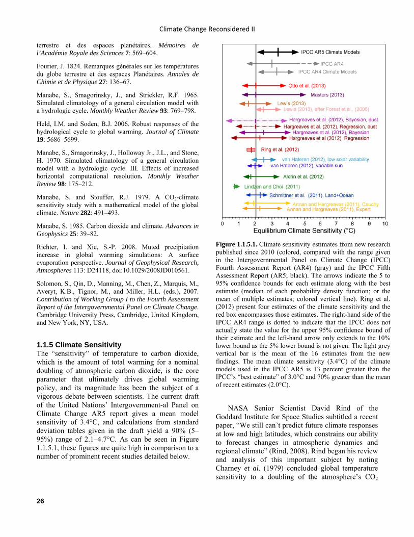
Climate Change Reconsidered II
26
terrestre et des espaces planétaires. Mémoires de l’Académie Royale des Sciences 7: 569–604.
Fourier, J. 1824. Remarques générales sur les températures du globe terrestre et des espaces Planétaires. Annales de Chimie et de Physique 27: 136–67.
Manabe, S., Smagorinsky, J., and Strickler, R.F. 1965. Simulated climatology of a general circulation model with a hydrologic cycle. Monthly Weather Review 93: 769–798.
Held, I.M. and Soden, B.J. 2006. Robust responses of the hydrological cycle to global warming. Journal of Climate 19: 5686–5699.
Manabe, S., Smagorinsky, J., Holloway Jr., J.L., and Stone, H. 1970. Simulated climatology of a general circulation model with a hydrologic cycle. III. Effects of increased horizontal computational resolution. Monthly Weather Review 98: 175–212.
Manabe, S. and Stouffer, R.J. 1979. A CO2-climate sensitivity study with a mathematical model of the global climate. Nature 282: 491–493.
Manabe, S. 1985. Carbon dioxide and climate. Advances in Geophysics 25: 39–82.
Richter, I. and Xie, S.-P. 2008. Muted precipitation increase in global warming simulations: A surface evaporation perspective. Journal of Geophysical Research, Atmospheres 113: D24118, doi:10.1029/2008JD010561.
Solomon, S., Qin, D., Manning, M., Chen, Z., Marquis, M., Averyt, K.B., Tignor, M., and Miller, H.L. (eds.), 2007. Contribution of Working Group I to the Fourth Assessment Report of the Intergovernmental Panel on Climate Change. Cambridge University Press, Cambridge, United Kingdom, and New York, NY, USA.
1.1.5 Climate Sensitivity The “sensitivity” of temperature to carbon dioxide, which is the amount of total warming for a nominal doubling of atmospheric carbon dioxide, is the core parameter that ultimately drives global warming policy, and its magnitude has been the subject of a vigorous debate between scientists. The current draft of the United Nations’ Intergovernment-al Panel on Climate Change AR5 report gives a mean model sensitivity of 3.4°C, and calculations from standard deviation tables given in the draft yield a 90% (5–95%) range of 2.1–4.7°C. As can be seen in Figure 1.1.5.1, these figures are quite high in comparison to a number of prominent recent studies detailed below.
NASA Senior Scientist David Rind of the Goddard Institute for Space Studies subtitled a recent paper, “We still can’t predict future climate responses at low and high latitudes, which constrains our ability to forecast changes in atmospheric dynamics and regional climate” (Rind, 2008). Rind began his review and analysis of this important subject by noting Charney et al. (1979) concluded global temperature sensitivity to a doubling of the atmosphere’s CO2
Figure 1.1.5.1. Climate sensitivity estimates from new research published since 2010 (colored, compared with the range given in the Intergovernmental Panel on Climate Change (IPCC) Fourth Assessment Report (AR4) (gray) and the IPCC Fifth Assessment Report (AR5; black). The arrows indicate the 5 to 95% confidence bounds for each estimate along with the best estimate (median of each probability density function; or the mean of multiple estimates; colored vertical line). Ring et al. (2012) present four estimates of the climate sensitivity and the red box encompasses those estimates. The right-hand side of the IPCC AR4 range is dotted to indicate that the IPCC does not actually state the value for the upper 95% confidence bound of their estimate and the left-hand arrow only extends to the 10% lower bound as the 5% lower bound is not given. The light grey vertical bar is the mean of the 16 estimates from the new findings. The mean climate sensitivity (3.4°C) of the climate models used in the IPCC AR5 is 13 percent greater than the IPCC’s “best estimate” of 3.0°C and 70% greater than the mean of recent estimates (2.0°C).

Global Climate Models and Their Limitations
27
concentration was “between 1.5° and 4.5°C,” while noting since then “we have not moved very far from that range.” In addition, Rind reported the uncertainty in our assessment of high- and low-latitude climate sensitivity “is also still as great as ever, with a factor of 2 at both high and low latitudes.”
Rind identifiend several problems contributing to the uncertainty. Whether the water vapor response to warming employed by climate models “is realistic is hard to assess,” he noted, “because we have not had recent climate changes of the magnitude forecast for the rest of this century” to test against. Closely associated are low-latitude difficulties related to modeling both low- and high-level clouds in the tropics and the physics and dynamics associated with them, plus high-latitude difficulties associated with cryosphere feedbacks related to sea ice and snow cover.
One way of dealing with these uncertainties has been to suggest, in Rind’s words, that “we can have greater confidence in the multi-model mean changes than in that of any individual model for climate change assessments.” However, he writes, “it is doubtful that averaging different formulations together will end up giving the ‘right’ result,” because “model responses (e.g., tropical land precipitation) can often be of different signs, and there can be little confidence that averaging them together will produce a better result.”
Rind thus concludes, “at this point, we cannot determine the low- and high-latitude sensitivities, and we have no real way of obtaining them.” These unknowns, in his opinion, “affect the confidence we can have in many of our projections of atmospheric dynamic and hydrologic responses to global warming.”
Because of these and a host of other complexities he discusses, Rind states, “forecasting even the large-scale response to climate change is not easy given the current uncertainties” and “regional responses may be the end result of varying influences in part due to warming in different tropical and high-latitude regions.”
Rind concludes “real progress will be the result of continued and newer observations along with modeling improvements based on these observations,” which observations must provide the basis for evaluating all model implications. So difficult is this task, however, that he says “there is no guarantee that these issues will be resolved before a substantial global warming impact is upon us.” There is, of course, also no guarantee there even will be any
“substantial global warming impact” from a doubling or more of the air’s CO2 content.
Lindzen and Choi (2009), two Massachusetts Institute of Technology scientists, used the National Centers for Environmental Prediction’s 16-year (1985–1999) monthly record of sea surface temperature (SST), together with corresponding radiation data from the Earth Radiation Budget Experiment, to estimate the sign and magnitude of climate feedback over the oceanic portion of the tropics and thus obtain an empirical evaluation of Earth’s thermal sensitivity, as opposed to the model-based evaluation employed by the IPCC.
The scientists found all 11 models employed in the IPCC’s analysis “agree as to positive feedback,” but they all disagree—and disagree “very sharply”—with the real-world observations Lindzen and Choi utilized, implying negative feedback actually prevails. Moreover, the presence of that negative feedback reduced the CO2-induced propensity for warming to the extent that their analysis of the real-world observational data yielded only a mean SST increase “of ~0.5°C for a doubling of CO2.”
Lindzen and Choi (2009) were criticized for not using available tropical high-altitude radiation data and for constraining feedback to within the tropics, which is highly unrealistic for a number of reasons, including Hadley Cell-westerly interactions and the export of large amounts of energy from the tropics into the temperate zone via tropical cyclones and poleward currents. They also did not explicitly use the IPCC-defined climate sensitivity.
However, Lindzen and Choi (2011) addressed these concerns by adding data from NASA’s Cloud and Earth Radiant Energy System (CERES), rather than simply using the older Earth Radiation Budget Experiment (ERBE) data. They also shared radiation feedback fluxes with the extratropics and addressed the sensitivity issues. The derived mean sensitivity was 0.7°, with a 90% range of 0.6–1.0°C, indicating virtually no positive amplification of warming beyond that from CO2.
Another empirically based analysis of climate sensitivity was published several years earlier in the review paper of Idso (1998), who described eight “natural experiments” he personally employed in prior studies designed to determine “how Earth’s near-surface air temperature responds to surface radiative perturbations.” The eight naturally occurring phenomena employed by Idso were (1) the change in the air’s water vapor content that occurs at Phoenix, Arizona, with the advent of the summer monsoon, (2)

Climate Change Reconsidered II
28
the naturally occurring vertical redistribution of dust that occurs at Phoenix between summer and winter, (3) the annual cycle of surface air temperature caused by the annual cycle of solar radiation absorption at Earth’s surface, (4) the warming effect of the entire atmosphere caused by its mean flux of thermal radiation to the surface of Earth, (5) the annually averaged equator-to-pole air temperature gradient sustained by the annually averaged equator-to-pole gradient of total surface-absorbed radiant energy, (6) the mean surface temperatures of Earth, Mars, and Venus relative to the amounts of CO2 contained in their respective atmospheres, (7) the paradox of the faint early Sun and its implications for Earth’s thermal history, and (8) the greenhouse effect of water vapor over the tropical oceans and its impact on sea surface temperatures.
These eight analyses, Idso writes, suggest “a 300 to 600 ppm doubling of the atmosphere’s CO2 concentration could raise the planet’s mean surface air temperature by only about 0.4°C,” in line with Lindzen and Choi’s deduced warming of ~0.5°C for a nominal doubling of the air’s CO2 content. There would thus appear to be strong real-world data that argue against the order of magnitude larger CO2 sensitivity predicted by state-of-the-art climate models.
Feedbacks are a natural part of the complexity of our climate system. They represent nonlinear processes within a system that are the result of the interaction between two or more variables or the interaction of a variable with itself (or its changes—“self” interaction) and influence overall climate sensitivity. Generally, these processes can only be parameterized, or represented in the models in an empirical way. Because of the inability to precisely represent feedbacks in a model, the model output may not be reasonable.
Temperature change in the climate system can be represented simply as a “forced-dissipative” relationship, for example by non-radiative and radiative processes as well as a net radiative restoring force, which is the feedback. As an example of this feedback process, if the system warms radiatively or non-radiatively, then the net radiative force may become negative (longwave-out increases and becomes larger than shortwave-in). Thus, the net radiative force will act to counter the warming, and a larger restoring force would represent a less-sensitive climate. The opposite can be argued for the system cooling. These principles can be represented by a simple differential or mathematical equation.
Investigating this subject further, a paper by Spencer and Braswell (2011) explored the sensitivity of the surface temperature response to a forced radiative imbalance. They used observed shortwave and longwave radiation gathered from satellite measurements and calculated the net atmospheric radiation. They also used observed surface temperatures from the years 2000–2010 around the globe and calculated global monthly temperature anomalies relative to the average over the ten-year period. Using these two time series, they correlated one versus the other using different time lags and compared these observed values to the same variables gathered from the twentieth century runs of the World Climate Research Programme (WCRP) Coupled Model Intercomparison Project (CMIP) phase 3 multi-model data set. The authors chose the three most- and least-sensitive model runs, rather than using all of them. They also used the observed and modeled data to investigate the mathematical relationship for temperature change described above.
When Spencer and Braswell set a “feedback” parameter as described above, they demonstrated that only for pure non-radiative forcing and with no time lag can the parameter be accurately diagnosed in the model (see Figure 1.1.5.1). With radiative forcing and a 70/30% mix of radiative versus non-radiative forcing, the response was quite different: “in this case, radiative gain precedes, and radiative loss follows a temperature maximum, as would be expected based upon conservation of energy considerations.” They also found, more importantly, that the pure radiative forcing curve in Figure 1.1.5.1 looks more like one produced using the data from the climate models, while the mixed curve looks more like that produced using the observed data.
Spencer and Braswell then point out, “we are still faced with a rather large discrepancy in the time-lagged regression coefficients between the radiative signatures displayed in the real climate system in satellite data versus the climate models.” Such discrepancy indicates the climate system possesses less sensitivity that the climate models project. That is, climate models may overestimate the temperature change forced by a certain process (e.g., increasing atmospheric CO2).
Further, it should be noted Earth’s climate is a complicated dynamic system in which each part has characteristic time- and space-scales over which it evolves, or as it reacts to a forcing that is external to that part of system or to the system as a whole. The atmosphere, being less massive than the ocean or the
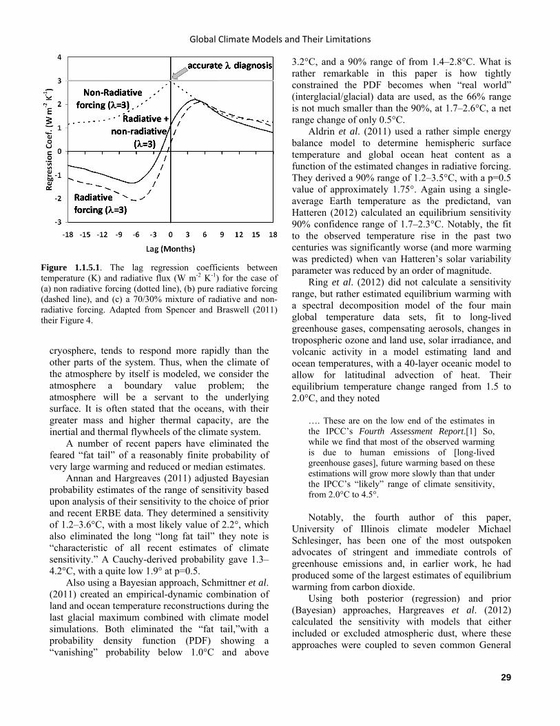
Global Climate Models and Their Limitations
29
cryosphere, tends to respond more rapidly than the other parts of the system. Thus, when the climate of the atmosphere by itself is modeled, we consider the atmosphere a boundary value problem; the atmosphere will be a servant to the underlying surface. It is often stated that the oceans, with their greater mass and higher thermal capacity, are the inertial and thermal flywheels of the climate system.
A number of recent papers have eliminated the feared “fat tail” of a reasonably finite probability of very large warming and reduced or median estimates.
Annan and Hargreaves (2011) adjusted Bayesian probability estimates of the range of sensitivity based upon analysis of their sensitivity to the choice of prior and recent ERBE data. They determined a sensitivity of 1.2–3.6°C, with a most likely value of 2.2°, which also eliminated the long “long fat tail” they note is “characteristic of all recent estimates of climate sensitivity.” A Cauchy-derived probability gave 1.3–4.2°C, with a quite low 1.9° at p=0.5.
Also using a Bayesian approach, Schmittner et al. (2011) created an empirical-dynamic combination of land and ocean temperature reconstructions during the last glacial maximum combined with climate model simulations. Both eliminated the “fat tail,”with a probability density function (PDF) showing a “vanishing” probability below 1.0°C and above
3.2°C, and a 90% range of from 1.4–2.8°C. What is rather remarkable in this paper is how tightly constrained the PDF becomes when “real world” (interglacial/glacial) data are used, as the 66% range is not much smaller than the 90%, at 1.7–2.6°C, a net range change of only 0.5°C.
Aldrin et al. (2011) used a rather simple energy balance model to determine hemispheric surface temperature and global ocean heat content as a function of the estimated changes in radiative forcing. They derived a 90% range of 1.2–3.5°C, with a p=0.5 value of approximately 1.75°. Again using a single-average Earth temperature as the predictand, van Hatteren (2012) calculated an equilibrium sensitivity 90% confidence range of 1.7–2.3°C. Notably, the fit to the observed temperature rise in the past two centuries was significantly worse (and more warming was predicted) when van Hatteren’s solar variability parameter was reduced by an order of magnitude.
Ring et al. (2012) did not calculate a sensitivity range, but rather estimated equilibrium warming with a spectral decomposition model of the four main global temperature data sets, fit to long-lived greenhouse gases, compensating aerosols, changes in tropospheric ozone and land use, solar irradiance, and volcanic activity in a model estimating land and ocean temperatures, with a 40-layer oceanic model to allow for latitudinal advection of heat. Their equilibrium temperature change ranged from 1.5 to 2.0°C, and they noted
…. These are on the low end of the estimates in the IPCC’s Fourth Assessment Report.[1] So, while we find that most of the observed warming is due to human emissions of [long-lived greenhouse gases], future warming based on these estimations will grow more slowly than that under the IPCC’s “likely” range of climate sensitivity, from 2.0°C to 4.5°. Notably, the fourth author of this paper,
University of Illinois climate modeler Michael Schlesinger, has been one of the most outspoken advocates of stringent and immediate controls of greenhouse emissions and, in earlier work, he had produced some of the largest estimates of equilibrium warming from carbon dioxide.
Using both posterior (regression) and prior (Bayesian) approaches, Hargreaves et al. (2012) calculated the sensitivity with models that either included or excluded atmospheric dust, where these approaches were coupled to seven common General
Figure 1.1.5.1. The lag regression coefficients between temperature (K) and radiative flux (W m-2 K-1) for the case of (a) non radiative forcing (dotted line), (b) pure radiative forcing (dashed line), and (c) a 70/30% mixture of radiative and non-radiative forcing. Adapted from Spencer and Braswell (2011) their Figure 4.

Climate Change Reconsidered II
30
Circulation Models (GCMs). The dust-free Bayesian model had the greatest sensitivity, with a range of 1.0–4.2°, with a central estimate of 2.4°C. The dust-included regression model yielded the smallest warming, a range of 0.8–3.4°C, with a central estimate of 2.0°C. The Bayesian dust-included model had a similar central estimate. Perhaps more important, Hargreaves et al. noted their collection of models yielded “a high probability of [equilibrium warming] lying below 4°C.”
Again coupling a Bayesian approach to a model, this time the MIT two-dimensional model, Lewis (2013) generated a 90% range of 1.0–3.0°C, with a central value of 1.6°C. Masters (2013) is the only recent sensitivity analysis based upon observed values of oceanic heat uptake, and he found a 90% sensitivity range of 1.2–5.1°, with a central value again of 2.0°C, substantially below what is in the suite of models employed in the existing draft of the IPCC’s Fifth Assessment Report.
Scaling the relationship between observed temperature in the widely cited HadCRUT4 temperature history with calculated changes in the total heat content of the Earth system, Otto et al. (2013) state their most reliable calculation yields a range of 1.2–3.9°C, centered on 2.0°C. The analogous range for the upcoming IPCC report is 2.2–4.7°C, centered on 3.4°C. This paper was authored by17 very prominent climate scientists.
Many of the senstitivity values are very similar to the twenty-first century warming Michaels et al. (2002) had projected some ten years earlier based largely on observational data, which may be the first of the low-sensitivity data-based papers in the literature.
In total, there are 42 researchers describing 19 separate experiments in this section.
In another paper, Olivé et al. (2012) examined the changes in global temperature relative to changes in CO2 concentration using two different models. This study also endeavored to quantify the uncertainties in the authors’ scenarios. The authors used output from the Hadley Centre’s Atmosphere-Ocean (UKMO-HadCM3) and the CNRM-CM3 Centre National de Recherches Meteorologiques Coupled Model, version 3 (CNRM-CM3) coupled Atmosphere Ocean General Circulation Models (AOGCMs). The simulations were relatively short, on the time scale of 100 to 300 years, since the model spatial resolution was higher. The authors also used CO2 scenarios where the increase was simulated to be sudden, corresponding to a 6.5 times increase (10 W/m2), a sudden doubling,
and then a gradual increase. The gradual increases (1% per year) resulted in a doubling and quadrupling of CO2 in 70 and 140 years, respectively. Additionally, the authors initially used a shorter (10 years) and long-scale (100 years) CO2 forcing as well as sensitivity values within the range of those given in the published literature for their a priori estimates. Then they solved the equations backward to get their estimates of the short- and long-time-scale modes and sensitivity.
The results from Olivé et al. (2012) show the short-time-scale temperature forcing for CO2 was on the order of three to four years, while it was 100 to 300 years on the long-time-scale. The shorter mode of temperature change was faster for the model simulations where the CO2 forcing was sudden (Figure 1.1.5.2) rather than the gradual CO2 increase simulations. The uncertainty also was lower for the sudden increase simulations. For the longer time-scale forcing, longer model integrations would be needed to estimate these and reduce the uncertainty. Concerning the model sensitivities, the authors write, “when assuming two modes it varies between 0.49 and 0.83 K W-1 m2 or between 0.56 and 1.01 K W-1 m2,” both within the published range shown early in the paper.
This kind of diagnostic work is an important use of long-term computer model simulations. Even though there is no predictive work being done in this study, it is remarkable that there is such variation in the estimate of the short- and long-term radiative forcing as well as in the climate sensitivity. This is especially true between the two models used. Such findings demonstrate the models are less than perfect, as any of these internal differences would have to be the result of the model physics employed, especially that pertaining to radiative forcing. Also, such long integrations should lead to the build-up of numerical errors. Lastly, the fact that the authors could not appreciably reduce the uncertainty in estimating these quantities indicates further improvement is not likely using the current technology.
References Aldrin, M., et al. 2012. Bayesian estimation of climate sensitivity based on a simple climate model fitted to observations of hemispheric temperature and global ocean heat content. Environmetrics, doi: 10.1002/env.2140.
Annan, J.D. and Hargreaves, J.D. 2011. On the generation and interpretation of probabilistic estimates of climate sensitivity. Climatic Change 104, 324–436.
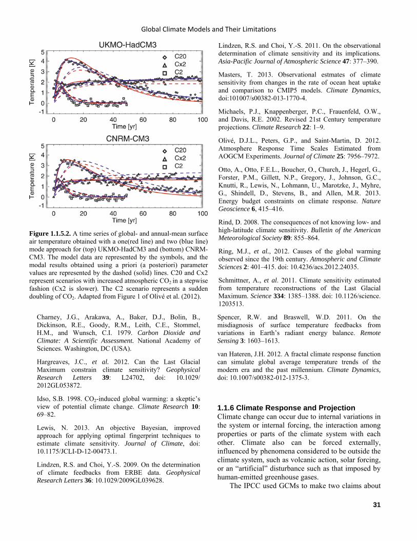
Global Climate Models and Their Limitations
31
Charney, J.G., Arakawa, A., Baker, D.J., Bolin, B., Dickinson, R.E., Goody, R.M., Leith, C.E., Stommel, H.M., and Wunsch, C.I. 1979. Carbon Dioxide and Climate: A Scientific Assessment. National Academy of Sciences. Washington, DC (USA).
Hargreaves, J.C., et al. 2012. Can the Last Glacial Maximum constrain climate sensitivity? Geophysical Research Letters 39: L24702, doi: 10.1029/ 2012GL053872.
Idso, S.B. 1998. CO2-induced global warming: a skeptic’s view of potential climate change. Climate Research 10: 69–82.
Lewis, N. 2013. An objective Bayesian, improved approach for applying optimal fingerprint techniques to estimate climate sensitivity. Journal of Climate, doi: 10.1175/JCLI-D-12-00473.1.
Lindzen, R.S. and Choi, Y.-S. 2009. On the determination of climate feedbacks from ERBE data. Geophysical Research Letters 36: 10.1029/2009GL039628.
Lindzen, R.S. and Choi, Y.-S. 2011. On the observational determination of climate sensitivity and its implications. Asia-Pacific Journal of Atmospheric Science 47: 377–390.
Masters, T. 2013. Observational estmates of climate sensitivity from changes in the rate of ocean heat uptake and comparison to CMIP5 models. Climate Dynamics, doi:101007/s00382-013-1770-4.
Michaels, P.J., Knappenberger, P.C., Frauenfeld, O.W., and Davis, R.E. 2002. Revised 21st Century temperature projections. Climate Research 22: 1–9.
Olivé, D.J.L., Peters, G.P., and Saint-Martin, D. 2012. Atmosphere Response Time Scales Estimated from AOGCM Experiments. Journal of Climate 25: 7956–7972.
Otto, A., Otto, F.E.L., Boucher, O., Church, J., Hegerl, G., Forster, P.M., Gillett, N.P., Gregory, J., Johnson, G.C., Knutti, R., Lewis, N., Lohmann, U., Marotzke, J., Myhre, G., Shindell, D., Stevens, B., and Allen, M.R. 2013. Energy budget constraints on climate response. Nature Geoscience 6, 415–416.
Rind, D. 2008. The consequences of not knowing low- and high-latitude climate sensitivity. Bulletin of the American Meteorological Society 89: 855–864.
Ring, M.J., et al., 2012. Causes of the global warming observed since the 19th century. Atmospheric and Climate Sciences 2: 401–415. doi: 10.4236/acs.2012.24035.
Schmittner, A., et al. 2011. Climate sensitivity estimated from temperature reconstructions of the Last Glacial Maximum. Science 334: 1385–1388. doi: 10.1126/science. 1203513.
Spencer, R.W. and Braswell, W.D. 2011. On the misdiagnosis of surface temperature feedbacks from variations in Earth’s radiant energy balance. Remote Sensing 3: 1603–1613.
van Hateren, J.H. 2012. A fractal climate response function can simulate global average temperature trends of the modern era and the past millennium. Climate Dynamics, doi: 10.1007/s00382-012-1375-3.
1.1.6 Climate Response and Projection Climate change can occur due to internal variations in the system or internal forcing, the interaction among properties or parts of the climate system with each other. Climate also can be forced externally, influenced by phenomena considered to be outside the climate system, such as volcanic action, solar forcing, or an “artificial” disturbance such as that imposed by human-emitted greenhouse gases.
The IPCC used GCMs to make two claims about
Figure 1.1.5.2. A time series of global- and annual-mean surface air temperature obtained with a one(red line) and two (blue line) mode approach for (top) UKMO-HadCM3 and (bottom) CNRM-CM3. The model data are represented by the symbols, and the modal results obtained using a priori (a posteriori) parameter values are represented by the dashed (solid) lines. C20 and Cx2 represent scenarios with increased atmospheric CO2 in a stepwise fashion (Cx2 is slower). The C2 scenario represents a sudden doubling of CO2. Adapted from Figure 1 of Olivé et al. (2012).
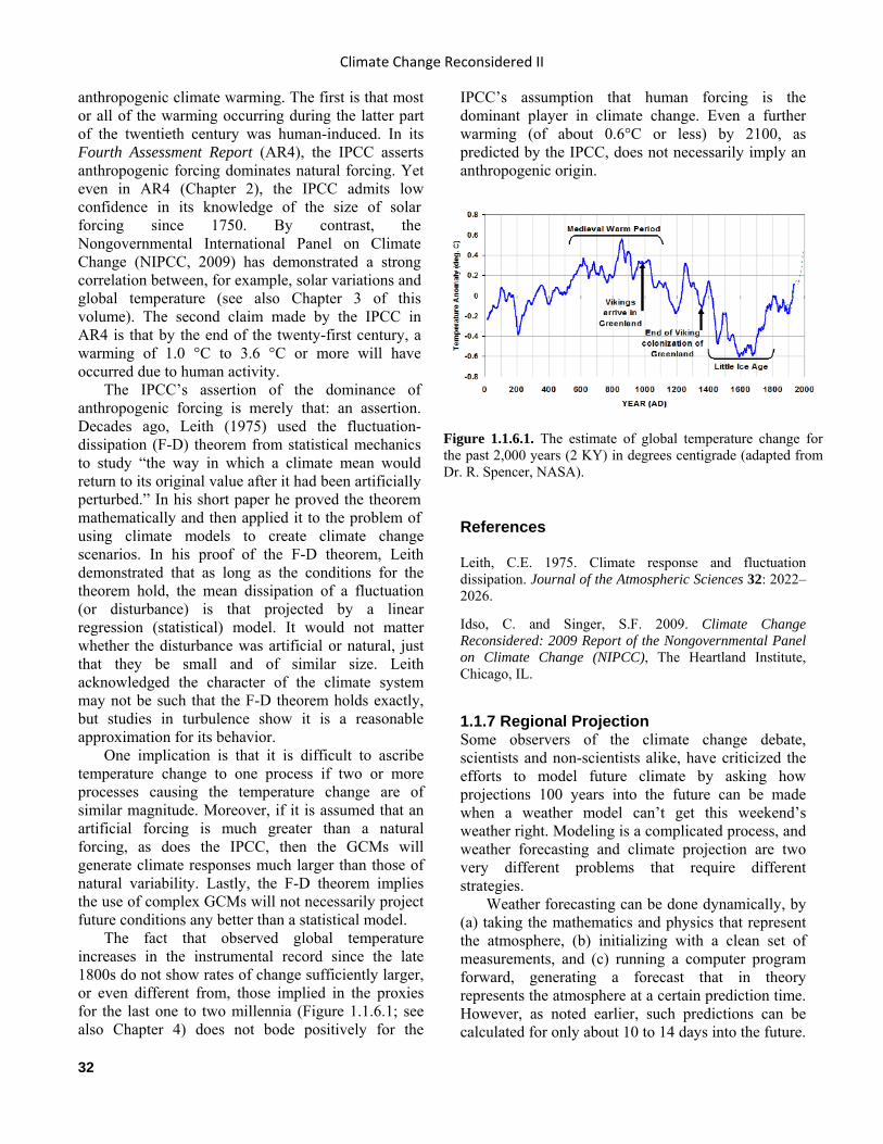
Climate Change Reconsidered II
32
anthropogenic climate warming. The first is that most or all of the warming occurring during the latter part of the twentieth century was human-induced. In its Fourth Assessment Report (AR4), the IPCC asserts anthropogenic forcing dominates natural forcing. Yet even in AR4 (Chapter 2), the IPCC admits low confidence in its knowledge of the size of solar forcing since 1750. By contrast, the Nongovernmental International Panel on Climate Change (NIPCC, 2009) has demonstrated a strong correlation between, for example, solar variations and global temperature (see also Chapter 3 of this volume). The second claim made by the IPCC in AR4 is that by the end of the twenty-first century, a warming of 1.0 °C to 3.6 °C or more will have occurred due to human activity.
The IPCC’s assertion of the dominance of anthropogenic forcing is merely that: an assertion. Decades ago, Leith (1975) used the fluctuation-dissipation (F-D) theorem from statistical mechanics to study “the way in which a climate mean would return to its original value after it had been artificially perturbed.” In his short paper he proved the theorem mathematically and then applied it to the problem of using climate models to create climate change scenarios. In his proof of the F-D theorem, Leith demonstrated that as long as the conditions for the theorem hold, the mean dissipation of a fluctuation (or disturbance) is that projected by a linear regression (statistical) model. It would not matter whether the disturbance was artificial or natural, just that they be small and of similar size. Leith acknowledged the character of the climate system may not be such that the F-D theorem holds exactly, but studies in turbulence show it is a reasonable approximation for its behavior.
One implication is that it is difficult to ascribe temperature change to one process if two or more processes causing the temperature change are of similar magnitude. Moreover, if it is assumed that an artificial forcing is much greater than a natural forcing, as does the IPCC, then the GCMs will generate climate responses much larger than those of natural variability. Lastly, the F-D theorem implies the use of complex GCMs will not necessarily project future conditions any better than a statistical model.
The fact that observed global temperature increases in the instrumental record since the late 1800s do not show rates of change sufficiently larger, or even different from, those implied in the proxies for the last one to two millennia (Figure 1.1.6.1; see also Chapter 4) does not bode positively for the
IPCC’s assumption that human forcing is the dominant player in climate change. Even a further warming (of about 0.6°C or less) by 2100, as predicted by the IPCC, does not necessarily imply an anthropogenic origin.
References Leith, C.E. 1975. Climate response and fluctuation dissipation. Journal of the Atmospheric Sciences 32: 2022–2026.
Idso, C. and Singer, S.F. 2009. Climate Change Reconsidered: 2009 Report of the Nongovernmental Panel on Climate Change (NIPCC), The Heartland Institute, Chicago, IL.
1.1.7 Regional Projection Some observers of the climate change debate, scientists and non-scientists alike, have criticized the efforts to model future climate by asking how projections 100 years into the future can be made when a weather model can’t get this weekend’s weather right. Modeling is a complicated process, and weather forecasting and climate projection are two very different problems that require different strategies.
Weather forecasting can be done dynamically, by (a) taking the mathematics and physics that represent the atmosphere, (b) initializing with a clean set of measurements, and (c) running a computer program forward, generating a forecast that in theory represents the atmosphere at a certain prediction time. However, as noted earlier, such predictions can be calculated for only about 10 to 14 days into the future.
Figure 1.1.6.1. The estimate of global temperature change for the past 2,000 years (2 KY) in degrees centigrade (adapted from Dr. R. Spencer, NASA).
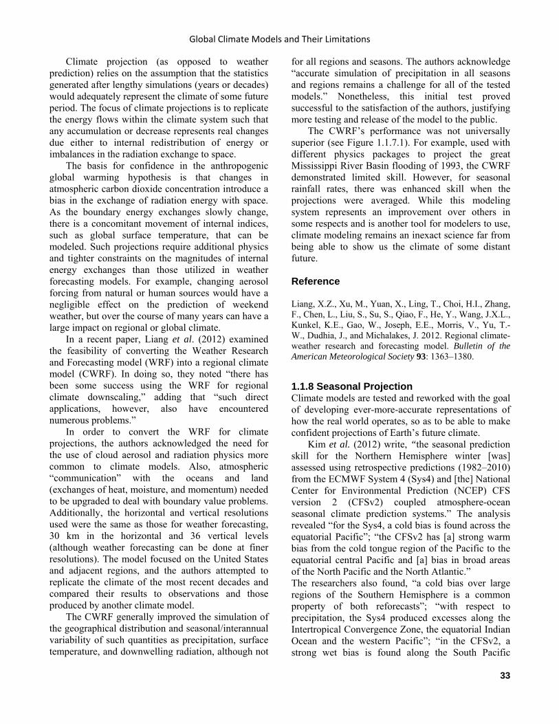
Global Climate Models and Their Limitations
33
Climate projection (as opposed to weather prediction) relies on the assumption that the statistics generated after lengthy simulations (years or decades) would adequately represent the climate of some future period. The focus of climate projections is to replicate the energy flows within the climate system such that any accumulation or decrease represents real changes due either to internal redistribution of energy or imbalances in the radiation exchange to space.
The basis for confidence in the anthropogenic global warming hypothesis is that changes in atmospheric carbon dioxide concentration introduce a bias in the exchange of radiation energy with space. As the boundary energy exchanges slowly change, there is a concomitant movement of internal indices, such as global surface temperature, that can be modeled. Such projections require additional physics and tighter constraints on the magnitudes of internal energy exchanges than those utilized in weather forecasting models. For example, changing aerosol forcing from natural or human sources would have a negligible effect on the prediction of weekend weather, but over the course of many years can have a large impact on regional or global climate.
In a recent paper, Liang et al. (2012) examined the feasibility of converting the Weather Research and Forecasting model (WRF) into a regional climate model (CWRF). In doing so, they noted “there has been some success using the WRF for regional climate downscaling,” adding that “such direct applications, however, also have encountered numerous problems.”
In order to convert the WRF for climate projections, the authors acknowledged the need for the use of cloud aerosol and radiation physics more common to climate models. Also, atmospheric “communication” with the oceans and land (exchanges of heat, moisture, and momentum) needed to be upgraded to deal with boundary value problems. Additionally, the horizontal and vertical resolutions used were the same as those for weather forecasting, 30 km in the horizontal and 36 vertical levels (although weather forecasting can be done at finer resolutions). The model focused on the United States and adjacent regions, and the authors attempted to replicate the climate of the most recent decades and compared their results to observations and those produced by another climate model.
The CWRF generally improved the simulation of the geographical distribution and seasonal/interannual variability of such quantities as precipitation, surface temperature, and downwelling radiation, although not
for all regions and seasons. The authors acknowledge “accurate simulation of precipitation in all seasons and regions remains a challenge for all of the tested models.” Nonetheless, this initial test proved successful to the satisfaction of the authors, justifying more testing and release of the model to the public.
The CWRF’s performance was not universally superior (see Figure 1.1.7.1). For example, used with different physics packages to project the great Mississippi River Basin flooding of 1993, the CWRF demonstrated limited skill. However, for seasonal rainfall rates, there was enhanced skill when the projections were averaged. While this modeling system represents an improvement over others in some respects and is another tool for modelers to use, climate modeling remains an inexact science far from being able to show us the climate of some distant future. Reference Liang, X.Z., Xu, M., Yuan, X., Ling, T., Choi, H.I., Zhang, F., Chen, L., Liu, S., Su, S., Qiao, F., He, Y., Wang, J.X.L., Kunkel, K.E., Gao, W., Joseph, E.E., Morris, V., Yu, T.-W., Dudhia, J., and Michalakes, J. 2012. Regional climate-weather research and forecasting model. Bulletin of the American Meteorological Society 93: 1363–1380.
1.1.8 Seasonal Projection Climate models are tested and reworked with the goal of developing ever-more-accurate representations of how the real world operates, so as to be able to make confident projections of Earth’s future climate.
Kim et al. (2012) write, “the seasonal prediction skill for the Northern Hemisphere winter [was] assessed using retrospective predictions (1982–2010) from the ECMWF System 4 (Sys4) and [the] National Center for Environmental Prediction (NCEP) CFS version 2 (CFSv2) coupled atmosphere-ocean seasonal climate prediction systems.” The analysis revealed “for the Sys4, a cold bias is found across the equatorial Pacific”; “the CFSv2 has [a] strong warm bias from the cold tongue region of the Pacific to the equatorial central Pacific and [a] bias in broad areas of the North Pacific and the North Atlantic.” The researchers also found, “a cold bias over large regions of the Southern Hemisphere is a common property of both reforecasts”; “with respect to precipitation, the Sys4 produced excesses along the Intertropical Convergence Zone, the equatorial Indian Ocean and the western Pacific”; “in the CFSv2, a strong wet bias is found along the South Pacific
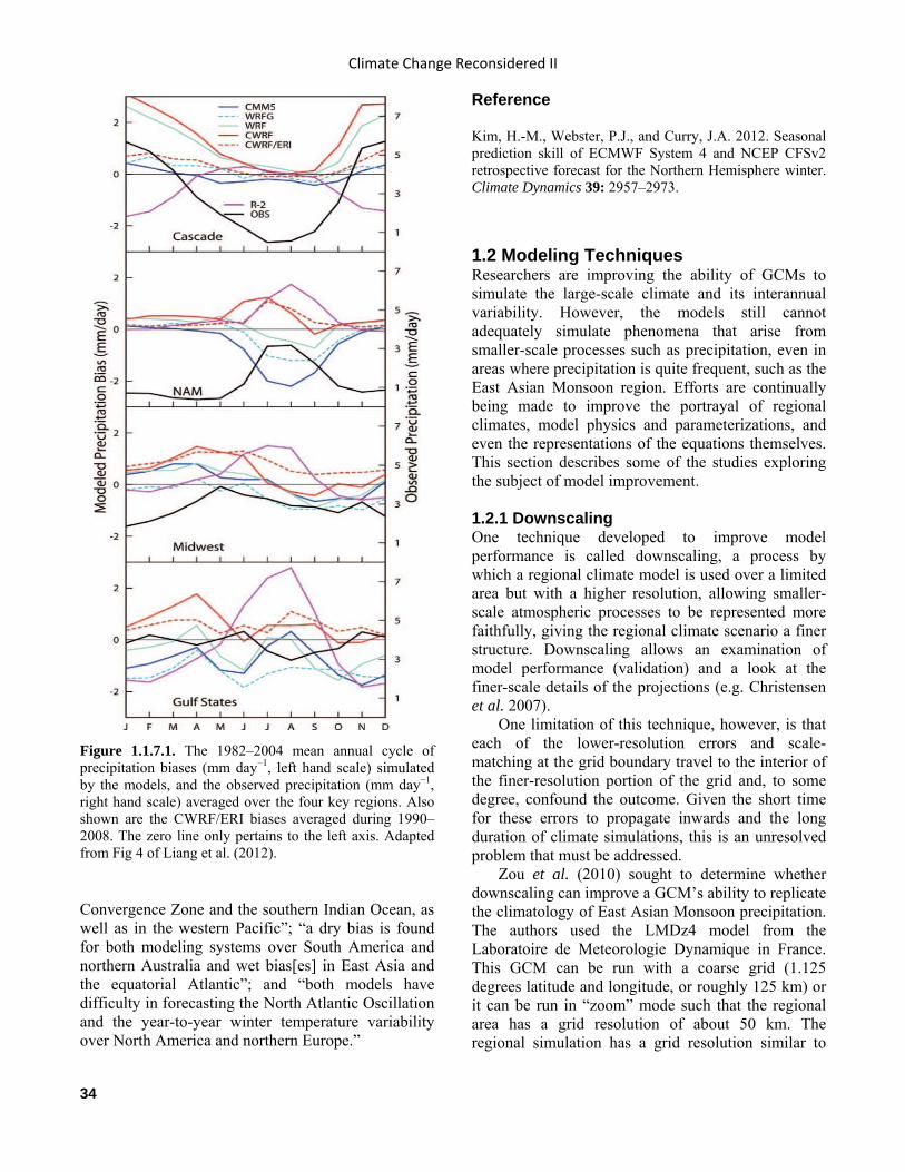
Climate Change Reconsidered II
34
Convergence Zone and the southern Indian Ocean, as well as in the western Pacific”; “a dry bias is found for both modeling systems over South America and northern Australia and wet bias[es] in East Asia and the equatorial Atlantic”; and “both models have difficulty in forecasting the North Atlantic Oscillation and the year-to-year winter temperature variability over North America and northern Europe.”
Reference Kim, H.-M., Webster, P.J., and Curry, J.A. 2012. Seasonal prediction skill of ECMWF System 4 and NCEP CFSv2 retrospective forecast for the Northern Hemisphere winter. Climate Dynamics 39: 2957–2973.
1.2 Modeling Techniques Researchers are improving the ability of GCMs to simulate the large-scale climate and its interannual variability. However, the models still cannot adequately simulate phenomena that arise from smaller-scale processes such as precipitation, even in areas where precipitation is quite frequent, such as the East Asian Monsoon region. Efforts are continually being made to improve the portrayal of regional climates, model physics and parameterizations, and even the representations of the equations themselves. This section describes some of the studies exploring the subject of model improvement. 1.2.1 Downscaling One technique developed to improve model performance is called downscaling, a process by which a regional climate model is used over a limited area but with a higher resolution, allowing smaller-scale atmospheric processes to be represented more faithfully, giving the regional climate scenario a finer structure. Downscaling allows an examination of model performance (validation) and a look at the finer-scale details of the projections (e.g. Christensen et al. 2007).
One limitation of this technique, however, is that each of the lower-resolution errors and scale-matching at the grid boundary travel to the interior of the finer-resolution portion of the grid and, to some degree, confound the outcome. Given the short time for these errors to propagate inwards and the long duration of climate simulations, this is an unresolved problem that must be addressed.
Zou et al. (2010) sought to determine whether downscaling can improve a GCM’s ability to replicate the climatology of East Asian Monsoon precipitation. The authors used the LMDz4 model from the Laboratoire de Meteorologie Dynamique in France. This GCM can be run with a coarse grid (1.125 degrees latitude and longitude, or roughly 125 km) or it can be run in “zoom” mode such that the regional area has a grid resolution of about 50 km. The regional simulation has a grid resolution similar to
Figure 1.1.7.1. The 1982–2004 mean annual cycle of precipitation biases (mm day−1, left hand scale) simulated by the models, and the observed precipitation (mm day−1, right hand scale) averaged over the four key regions. Also shown are the CWRF/ERI biases averaged during 1990–2008. The zero line only pertains to the left axis. Adapted from Fig 4 of Liang et al. (2012).

Global Climate Models and Their Limitations
35
that of a weather forecast model. Zou et al. ran the model for the East Asia Region
for the years 1958–2000 in order to compare the modeled climate to monthly observations from this region over the same time period. The raw output revealed the model produced more (less) precipitation when downscaling was (not) used. When the authors extracted the larger-scale component of the precipitation signal from the precipitation data (Figure 1.2.1.1), they found the model results without downscaling were unable to adequately represent the monsoon pattern or its variability (compare Figure 1.2.1.1 frames a, b to frames e, f). The downscaling results (Figure 1.2.1.1 frames c, d) compared more favorably.
Even though the results were an improvement, flaws remained. As Zou et al. point out, “it should be acknowledged that our results of dynamic downscaling are not perfect,” while adding “the main weakness of the downscaling is the northward shift of the monsoon rainbelt.” Although downscaling improves some aspects of the performance of models and their ability to represent observations, this technique is still subject to the general limitations suffered by all numerical models.
Indeed, numerous errors permeate numerical models for both weather forecasts and climate projections. These fall under three headings, (1) observational error, (2) numerical error, and (3) physical error.
Observational error refers to the fact that instrumentation cannot measure the state of the atmosphere with infinite precision; it is important both for establishing the initial conditions and validation. Numerical error covers many shortcomings including “aliasing,” the tendency to misrepresent the sub-grid scale processes as larger-scale features. In the downscaling approach, presumably errors in the large-scale boundary conditions also will propagate into the nested grid. Also, the numerical methods themselves are only approximations to the solution of the mathematical equations, and this results in truncation error. Physical errors are manifest in parameterizations, which may be approximations, simplifications, or educated guesses about how real processes work. An example of this type of error would be the representation of cloud formation and dissipation in a model, which is generally a crude approximation.
Each of these error sources generates and propagates errors in model simulations. Without some “interference” from model designers, model solutions
accumulate energy at the smallest scales of resolution or blow up rapidly due to computational error. In weather prediction, techniques have been developed to “smooth” and massage the data during a simulation by removing as much grid-scale energy as possible while retaining the character of the larger scale. Nonetheless, computational error does prevent models from forecasting perfectly, and this explains why two different models (or even two different runs with the same model) can give two different answers given the same or similar set of initial conditions.
Otte et al. (2012) use a technique called “nudging” to improve the performance of a weather forecasting model (Weather Research and Forecasting model—WRF) for use in downscaling. Nudging is used to keep the regional model results within the bounds of the larger-scale model results.
Generally applied to the boundaries of a model,
Figure 1.2.1.1. The strongest (left) and second strongest (right) component of summer season precipitation shown as a percentage from the rain gauge observations (top), the GCM with downscaling (middle), and the GCM without downscaling (bottom). Darker (lighter) colors represent more (less) precipitation than the actual measurements. Adapted from Figure 4 in Zou et al. (2010).

Climate Change Reconsidered II
36
Otte et al. applied the nudging technique to the interior of the grids. To test the procedure, they used a coarse analysis data set from the National Centers for Environmental Prediction to initialize the regional model. These analyses stood as a proxy for GCM output. They then compared their results to two fine-scale regional re-analyses for North America.
This modeling technique generated a better representation of monthly means and improved interannual variability. The simulations of hot and cold extremes, as well as wet and dry extremes, were captured better in the nudged WRF. However, Otte et al. note, “all WRF runs overpredicted precipitation totals through the multidecadal period … regardless of whether nudging was used” (see Figure 1.2.1.2). Fewer false alarms of severe precipitation events were produced with the nudging technique than when it was not used, an important result given that most impacts on society result from the occurrence of extreme events. Reliable simulations that include the realistic occurrence of extremes are valuable for economic planners.
In spite of the success of the nudging employed by Otte et al. (2012), their results demonstrate modeling today’s climate cannot be done either on the largest scales or regionally without some way of “tuning” the model. This entails using parametric means to force the model to adequately represent reality. Although downscaling can be a valuable tool for regional climate simulations, this newfound ability
is meaningless if the GCM results that are being downscaled are themselves unrealistic. References Christensen, J.H., Hewitson, B., Busuioc, A., Chen, A., Gao, X., Held, I., Jones, R., Kolli, R.K., Kwon, W.-T., Laprise, R., Magaña Rueda, V., Mearns, L., Menéndez, C.G., Räisänen, J., Rinke, A., Sarr, A., and Whetton, P. 2007. Regional Climate Projections. In: Climate Change 2007: The Physical Science Basis. Contribution of Working Group I to the Fourth Assessment Report of the Intergovernmental Panel on Climate Change. Solomon, S., Qin, D., Manning, M., Chen, Z., Marquis, M., Averyt, K.B., Tignor, M., and H.L. Miller (eds.). Cambridge University Press, Cambridge, United Kingdom and New York, NY, USA.
Otte, T.L., Nolte, C.G., Otte, M.J., and Bowden, J.H. 2012. Does nudging squelch the extremes in regional climate modeling? Journal of Climate 25: 7046–7066.
Zou, L., Zhou, T., Li, L., and Zhang, J. 2010. East China summer rainfall variability of 1958–2000: Dynamical downscaling with a variable resolution AGCM. Journal of Climate 23: 63946408.
1.2.2 The Dynamic Core An atmospheric model, whether a forecast model or one used to diagnose which processes drive the climate, is built on a foundation of three main conservation principles: Within the Earth-atmosphere
Figure 1.2.1.2. The annual area-averaged number of days with (a) precipitation greater than (a) 0.5 in, and (b) 1.0 in for the Midwest region. Data are shown from North American Regional Reanalyses (O) and WRF runs for no nudging (N), nudging toward analyses (A), and spectral nudging (S). Adapted from Figure 13 in Otte et al. (2012).

Global Climate Models and Their Limitations
37
system, mass, energy, and momentum must be conserved. These basic physical principles are represented by a closed set of equations termed the primitive equations. The equations form the “dynamic core” of climate models and represent the motions of air within the model. The model output is generally some variable representing mass (pressure), temperature, or both.
The primitive equations are too complex in their raw form to be represented adequately in models and are often simplified following the concept of Occam’s Razor: They are simplified as much as possible, and no more. One way these equations have been simplified is to “linearize” them, thereby eliminating nonlinearity that can make a computer model unstable. This nonlinearity is a process by which the atmosphere behaves in a chaotic fashion. It is also the reason computational errors propagate and amplify. The falsely generated energy interacts across all scales of motion to distort the path of the model evolution such that eventually the scales of motion of interest (weather systems) have only limited forecast relationship to that of the atmosphere they are attempting to reproduce. This is the predictability barrier.
Kondrashov et al. (2011) used a simplified three-level atmospheric circulation model designed by
Marshall and Molteni (1993) to show the evolution of the wind fields. The model has a fairly coarse horizontal and vertical resolution by today’s standards, but it has been shown to represent the largest scales of the atmosphere’s climate in a fairly realistic way. The experiment here examined the tendencies of the 500 hPa mass field (streamfunction) due to linear and nonlinear processes. The nonlinear processes were divided into those that are resolvable by the model and those that are of smaller scale than can be represented by the model.
The model output was slightly different depending on which processes were included in the model run. A comparison of the full nonlinear processes or interactions (Figure 1.2.2.1a) gave slightly different results than when comparing only nonlinear resolvable processes (Figure 1.2.2.1b). The model output also differed from that of two similar studies because of the strategies used to calculate these model “climates.” The authors conclude the article by stating “the manner of defining interactions between the resolved and unresolved modes plays a crucial role in the dynamical interpretation of the tendency-based statistical diagnostics.”
The basic lesson to be learned from the authors’ closing statement is that there can be output differences produced within the same model core
Figure 1.2.2.1. The mean tendencies (model output) in the phase space (mathematical space, not physical), for (a) tendencies due to the full nonlinear processes,( b) nonlinear processes that are resolvable, (c) the linear inverse model output, and (d) the linear part of the nonlinear tendencies. Adapted from Kondrashov et al. (2011).
Climate Change Reconsidered II
38
even when using the same input data, depending on how the nonlinear processes are represented. If the representation of climate can be different depending on how these core processes are represented, then producing model scenarios on the time scale of a century must be done very cautiously and interpretation of the results done carefully.
References Kondrashov, D., Kravtsov, S., and Ghil, M. 2011. Signatures of nonlinear dynamics in an idealized atmospheric model. Journal of the Atmospheric Sciences 68: 3–12.
Marshall, J. and Molteni, F. 1993. Toward a dynamical understanding of atmospheric weather regimes. Journal of the Atmospheric Sciences 50: 1972–1818.
1.2.3 Statistical Models 1.2.3.1 Statistical Validation The Intertropical Convergence Zone (ITCZ) is an important feature in the atmosphere’s general circulation. The ITCZ is a belt of low pressure near the equator where the northeast and southeast trade winds from the Northern and Southern Hemispheres converge. The ITCZ is also characterized by light winds and intermittent regions of convective activity. In some parts of the globe it is easy to identify and in other parts it is more difficult, as it is ill-defined.
This feature is important to the climate system because convection in the ITCZ is the vehicle by which the excess heat and momentum of the tropics begins the journey poleward so as to keep the energetics of the climate system in balance. The ITCZ, which migrates northward in the tropics from January to July (and back southward in July to January), is also an important contributor to the occurrence of the monsoons and often serves as the producer of seed disturbances that become tropical cyclones. Thus it would be important for any study of climate to be able to identify and understand the dynamics of this feature.
Bain et al. (2011) used satellite data to develop a modeling tool that can be used to objectively and reliably locate the ITCZ. They used images derived from reflected light (visible—VIS) and radiated energy (infrared images—IR) from Earth. They also used images generated by the intensity of microwave emission and measuring the return (water vapor depth
–WV). They limited their domain to the Eastern Pacific from the International Dateline to South America, over the period 1995–2008.
In the model, the presence of the ITCZ was inferred based on the most likely location prior to analysis. Then a point was labeled as ITCZ or non-ITCZ by testing the value of the satellite data typical for the ITCZ, as well as the status of the surrounding grid points in both time and space. A second pass of the dataset blended the a priori information with the satellite data and the likelihood that a particular point was ITCZ or non-ITCZ. The method was then evaluated against manual observation and identification of the ITCZ (see Figure 1.2.3.1.1).
The Bain et al. study revealed the statistical methodology tested very well in objectively identifying the ITCZ and was subsequently used to
Figure 1.2.3.1.1. The ITCZ cloudiness for 2100 UTC 19 August 2000 overlaid on the IR data for (a) the manual detection, (b) the statistical model from the IR, VIS, and WV satellite data, and (c) the threshold at 270 Kelvin without post-processing. The gray-scale bar below represents the temperatures in the image, and the bold contour in (a) and (b) the position of the ITCZ. Adapted from Figure 3 in Bain et al. (2011).

Global Climate Models and Their Limitations
39
examine the climatological characteristics of the ITCZ. The seasonal evolution of the ITCZ as determined by the methodology showed it migrated with the seasons and its passage followed the seasonal location for the regions of warm sea surface temperatures (SSTs). In order to look at the climatological trends and interannual variations, Bain et al. extended the satellite data set back to 1980 for the IR data only. In doing so they found there was enhanced (less) ITCZ convection in El Niño (La Niña) years, a finding reached in previous studies. However, they found “no climatic shifts in the position of the ITCZ could be detected,” which suggests, they write, “any trends in the ITCZ location over the 30 years (that are not due to ENSO) are quite small or non-existent.”
Thus, statistical modeling can be used to objectively identify, in more detail, important features of the general circulation that we previously thought were well-known. The successful design of a model to objectively locate the ITCZ will be useful in the future study of its dynamics as well as its interaction with other tropical features such as the monsoons or the Madden Julian Oscillation (MJO), which manifests as a 30- to 60-day oscillation in tropical convection. Not all models are dynamic, and not all models are used to project the future climate. But using this particular model, Bain et al. showed no significant change in the character of the ITCZ in the past 30 years over the tropical Eastern Pacific. Reference Bain, C.L., J. DePaz, J. Kramer, G. Magnusdottir, P. Smyth, H. Stern, and C.-C. Wang, 2011. Detecting the ITCZ in instantaneous satellite data using spatiotemporal statistical modeling: ITCZ climatology in the East Pacific. Journal of Climate 24: 216–230.
1.2.3.2 Empirical Models Models can be analytical, statistical, or empirically derived and are then used to examine trends or cycles in a time series in an effort to determine the causes of change or variability.
Loehle and Scafetta (2011) built a one-dimensional model of global temperatures from 1850 to 2010 using the inductive approach and used this model to project the change in climate from the current time to the year 2100. The authors constructed their model using what they called “decomposition analysis,” based on a method of cycles and used in
identifying cyclic behavior in a time series. Previous research from each author and their
colleagues had found there are cyclic and quasi-cyclic forcing processes that can be extracted from local and global time series of temperature. Such cycles can be related to solar and astronomical activity (for example 11, 22, 50–80 years; see Chapter 3 of this volume), or terrestrial oscillations such as the Pacific Decadal Oscillation (about 60 years). Their earlier research pointed to the presence and dominance of 20- and 60- year cycles in temperature time series. Their model also identified a linear trend that may be related to solar and volcanic activity since the middle of the Little Ice Age. Additionally, they included an anthropogenic trend emerging in the early 1940s (Figure 1.2.3.2.1). These four processes combined to produce a model that fit the global temperature series from 1850 to 2010 very well.
Loehle and Scafetta determined that more than 50 percent and as much as 60 percent of the climate signal from 1850 to 2010 was the product of natural forcing. They projected future climate to the year 2100 using the model, stating, “the result is a continued warming with oscillations to a high in 2100 of about 0.6°C above 2000 values.” This resulted from the combined effect of natural and anthropogenic forcing.
The 0.6°C temperature rise projected by the Loehle and Scafetta model is much less than the low-end estimates of 2.3°C projected by the GCMs relied upon by the IPCC and is consistent with recent estimates of low climate sensitivity. Also, the Loehle and Scafetta model shows the latest downturn in temperatures since 2000. The IPCC (2007) models do not show this downturn and assume 90 percent or more of the climate change since 1970 is anthropogenic. As Loehle and Scafetta point out, “we have shown that the effect of natural oscillations is critical for proper assessment of anthropogenic impacts on the climate system.” Perhaps this is why Loehle and Scafetta’s model fits the historic temperature data much better than do most of the IPCC models, and with far fewer parameters.
Several studies have shown GCMs are improving in their ability to reproduce the current climate, including intraseasonal and interannual variations. The ability of the GCMs to capture internal nonlinear processes, however, will always be suspect.
But when examining climate, important external forcing processes need to be accounted for, including such natural processes as volcanic activity and solar variations. There is increasing evidence that

Climate Change Reconsidered II
40
extraterrestrial forcing processes can have an impact on solar variations and, thus, terrestrial climate.
Recent work by Scafetta (2011) explores several such issues. First, the author expanded on his own work demonstrating a link between well-known climate cycles of roughly 10, 20, and 60 years to celestial cycles. The celestial cycles result from the solar-lunar tidal oscillation (9.1 years) and gravitational cycles related to the interaction between the sun and the largest planets (Jupiter and Saturn). These celestial cycles have periods of about 10, 20, and 60 years. Loehle and Scafetta (2011) demonstrated these cycles can be added together and, with a realistic anthropogenic effect, reconstruct the global climate record since 1950. They also show this
empirical model can be used to project climate into the twenty-first century.
Scafetta also demonstrated the IPCC GCMs cannot capture decadal and interdecadal variability. As shown by the author (see Figure 1.2.3.2.2), “although these GCM simulations present some kind of red-noise variability supposed to simulate the multi-annual, decadal, and multidecadal natural variability, a simple visual comparison among the simulations and the temperature record gives a clear impression that the simulated variability has nothing to do with the observed temperature dynamics.”
Scafetta then demonstrates natural variability is not solely the result of internal variations; the external forcing described above also plays a role. These external forcings modulate solar output, which in turn impacts electrical activity in the upper atmosphere. This influences incoming cosmic ray fluxes, which have been linked to variability in cloudiness. The external cycles have periods similar to internal climate variations. Natural variations then, likely account for more than half the climate variability since 1850.
Finally, Scafetta also demonstrated the IPCC is erroneous in ascribing nearly all of the twentieth and twenty-first century climate change to anthropogenic forcing. When the anthropogenic effect is corrected, it accounts for less than half the recent climate change. Scafetta also showed the empirical model in his paper projected the cooling of the most recent decade, whereas the IPCC GCMs produced a quasi-monotonic warming of the climate from about the year 2000 on. Scafetta’s model produces a warming of only 0.8–1.5o C by the end of the twenty-first century.
Scientists skeptical of the IPCC’s projections of anthropogenic climate change have cautioned the public about the shortcomings of the IPCCs reliance on GCMs in producing climate change scenarios for the next century. In addition to well-documented problems with model numerics, the lack of data, and chaos, the physics of the models fall short. This is true not only for such internal processes as cloud physics, but also for such external forcing as Sun-moon tidal forcing and other solar system gravitational cycles that influence solar output.
Scafetta’s work demonstrates there is increasing evidence our solar system plays a significant role in decadal and multidecadal climate variations. The climate projections produced by Scafetta’s empirical harmonic model may be far more realistic and are certainly more optimistic.
Figure 1.2.3.2.1. (Top) A full reconstruction of the global temperature anomaly (°C) record of 1850 -2010 using the model described by Loehle and Scafetta (2011). (Bottom) The individual components of the model, where the solid line is the long term trend and the dashed line is the anthropogenic component. Adapted from Figure 3 in Loehle and Scafetta (2011).

Global Climate Models and Their Limitations
41
References IPCC. 2007. Climate Change 2007 -I: The Science of Basis, Contributions of Working Group I to the Fourth Assessment Report of the Intergovernmental Panel on Climate Change. Edited by: Solomon, S., Qin, D., Manning, M., Marquis, M., Averyt, K, Tignor, M.M.B., Miller, H.L. Jr., and Chen, Z.. Cambridge University Press, Cambridge, UK.
Loehle, C. and Scafetta, N. 2011. Climate change attribution using empirical decomposition of climatic data. The Open Atmospheric Science Journal 5: 74–86.
Scafetta, N. 2011. Testing an astronomically based decadal-scale empirical harmonic climate model versus the IPCC (2007) general circulation models. Journal of Atmospheric and Solar-Terrestrial Physics 80: 124–137.
1.2.4 Low Order Models In meteorology it is well-known that the limit of dynamic predictability is approximately 10 to 14 days. This constraint is imposed by the composition of our atmosphere and the size of the planet. However, there has been some disagreement in the climate community over whether there is a fair amount of predictability in climate or whether it is too chaotic for meaningful prediction. It is appropriate here to revisit a classic work written by E.N. Lorenz nearly 50 years ago on the subject of predictability in atmospheric flows.
At the time, meteorology was interested in explaining why the mid-latitude flow (jet stream) would transition from a higher amplitude state to a more zonal state in an irregular fashion at a time scale of roughly 10 to 14 days. There was also some interest in being able to make monthly and seasonal forecasts, which during the late 1950s to 1960s were considered very long range. During this time, numerical weather prediction was also in its infancy.
Lorenz (1963) was expressly interested in examining the behavior of periodic and non-periodic flows. Later Lorenz would describe the non-periodic behavior as “chaos,” which he then termed “order without periodicity.”
He used a technique called low order modeling to study the behavior of convection in a geophysical fluid. To do so he coupled the Equation of Motion and the First Law of Thermodynamics and then represented the motion and temperature variables in terms of waves, which were then characterized by the lowest wave numbers that reasonably represented these fields. He was able to demonstrate the solutions for the system in mathematical space and thus follow the evolution of the system in time. The resultant graph is commonly known today as Lorenz’s butterfly (Figure 1.2.4.1). He realized this model provided a good analogue for the behavior of mid-latitude flow.
In theory, then, if we know the precise initial conditions of the system such that we lay on one of the trajectories in the “butterfly,” we could follow that
trajectory forever and know what the state of the weather would be into the future infinitely.
Figure 1.2.3.2.2. The global surface temperature taken from http://www.cru.uea.ac.uk/cru/data/temperature/ (black) and the GISS ModelE average simulation (blue), and a fit using an empirical harmonic model (red). Adapted from Scafetta (2011) Figure 1.
Figure 1.2.4.1. A representation of Lorenz’s butterfly developed using the model published in Lorenz (1963). This picture was adapted from an Internet image.
Climate Change Reconsidered II
42
Computers could then make weather or climate forecasts, and meteorologists would be out of jobs.
However, even today’s best models are comprised only of hypotheses about how scientists believe the atmosphere really works. As the past has made abundantly clear, state-of-the-art models of “today” quickly outlive their usefulness and are eventually replaced by the newer and improved models of “tomorrow.” Today’s best representation of the physics is inadequate and there are also numerical model errors, in that differential quantities can only be estimated.
But the crux of predictability rests in the fact that the initial conditions are not precisely known. There is always a degree of uncertainty within them, and thus it is not known on which trajectory the model rests. According to Lorenz, “when our results concerning the instability of non-periodic flow are applied to the atmosphere, which is ostensibly nonperiodic, they indicate that prediction of the sufficiently distant future is impossible by any method, unless the present conditions are known exactly. In view of the inevitable inaccuracy and incompleteness of weather observations, precise very-long-range forecasting would seem to be non-existent.” The problem of not being able to specify the precise initial state—sensitive dependence on initial conditions (SDIC)—is an integral characteristic of chaotic systems.
Lorenz’s statement makes it plain that beyond 10 to 14 days, the typical timescale for the evolution of the mid-latitude flow, dynamic predictability is impossible. This is true in spite of the fact we can specify the equations representing motions in the flow. Such limits on predictability are thus scale-dependent. For example, because of their small spatial scales, we cannot dynamically predict the occurrence of individual thunderstorms beyond the 30- to 120- minute time-scale it takes for them to evolve. Beyond the time limits, corresponding to the appropriate space-scale, only statistical prediction is useful.
One way modelers attempt to mitigate SDIC is via the use of ensemble modeling. The technique is to take the initial conditions and several plausible alternative initial conditions (but very close by to the original) and run the model several times using each set. If the trajectories all evolve toward a common trajectory, the modelers claim there is high confidence that the predicted solution is highly probable. But when these trajectories diverge (another characteristic of chaotic systems), the probability that any one of them will be the actual prediction is small.
Model runs of climate change scenarios exhibit this latter behavior. In these projections, the spread in the forecasts gets larger and larger as the projection time horizon lengthens. This is exactly the behavior expected from models attempting to simulate nonlinear flow—the energy of eddies below the grid scale appears chaotically as eddies on scales of the motion resolved by the grid.
Thus there is ample evidence the climate behaves in a chaotic way and climate prediction is simply not possible; only the development of scenarios is possible. Although these scenarios might be statistically similar to the real climate (as opposed to accurate in detail), this observation remains to be demonstrated and cannot be assumed.
Reference Lorenz, E.N. 1963. Deterministic nonperiodic flow. Journal of Climate 20: 130–139.
1.2.5 Bias Correction In a Hydrology and Earth System Sciences opinion article, Ehret et al. (2012) write, “despite considerable progress in recent years, output of both global and regional circulation models is still afflicted with biases to a degree that precludes its direct use, especially in climate change impact studies,” noting “this is well known, and to overcome this problem, bias correction (BC, i.e., the correction of model output towards observations in a post-processing step) has now become a standard procedure in climate change impact studies.” For example, GCMs often produce a global climate that is too cool or too warm by several degrees compared to the real world.
Ehret et al. present “a brief overview of state-of-the-art bias correction methods, discuss the related assumptions and implications, draw conclusions on the validity of bias correction and propose ways to cope with biased output of circulation models.”
In discussing the findings of their review, the authors state: (1) “BC methods often impair the advantages of circulation models by altering spatiotemporal field consistency, relations among variables and by violating conservation principles,” (2) “currently used BC methods largely neglect feedback mechanisms, (3) “it is unclear whether they are time-invariant under climate change conditions,” (4) “applying BC increases agreement of climate model output with observations in hindcasts and hence narrows the uncertainty range of simulations

Global Climate Models and Their Limitations
43
and predictions,” but (5) this is often done “without providing a satisfactory physical justification,” and this sleight of hand “is in most cases not transparent to the end user.” For example, the temperatures produced by GCMs are presented as anomalies in the IPCC reports so their disagreement with each other and with the real world are hidden.
Ehret et al. argue this set of negative consequences of bias correction “hides rather than reduces uncertainty,” which they suggest may lead to avoidable forejudging of end users and decision makers. They conclude BC is often “not a valid procedure.” Reference Ehret, U., Zehe, E., Wulfmeyer, V., Warrach-Sagi, K., and Liebert, J. 2012. Should we apply bias correction to global and regional climate model data? Hydrology and Earth System Sciences 16: 3391–3404.
1.3 Elements of Climate GCMs must incorporate all the many physical, chemical, and biological processes that influence climate over different spatial and temporal scales. Although the models have evolved much in recent years, limitations and deficiencies remain.
Many important processes are either missing or inadequately represented in today’s state-of-the-art climate models. Here we highlight many of the insufficiencies researchers have found when comparing model projections against real-world observations, frequently using the researchers’ own words to report them. The list is long and varied, and it demonstrates much work remains to be done before the model simulations can be treated with the level of confidence ascribed to them by the IPCC. 1.3.1 Radiation One of the most challenging and important problems facing today’s general circulation models of the atmosphere is how to accurately simulate the physics of Earth’s radiative energy balance. In commenting on this task, Harries (2000) stated more than a decade ago, “progress is excellent, on-going research is fascinating, but we have still a great deal to understand about the physics of climate.” He added, “we must exercise great caution over the true depth of our understanding, and our ability to forecast future climate trends.” As an example, he points out our knowledge of high cirrus clouds is very poor (it
remains so today), noting “we could easily have uncertainties of many tens of W m-2 in our description of the radiative effect of such clouds, and how these properties may change under climate forcing.”
Potential errors of this magnitude are extremely disconcerting in light of the fact that the radiative effect of a doubling of the air’s CO2 content is in the lower single-digit range of Wm-2, and, to quote Harries, “uncertainties as large as, or larger than, the doubled CO2 forcing could easily exist in our modeling of future climate trends, due to uncertainties in the feedback processes.”
Furthermore, because of the vast complexity of the subject, Harries declares, “even if [our] understanding were perfect, our ability to describe the system sufficiently well in even the largest computer models is a problem.”
Illustrative of a related problem is the work of Zender (1999), who characterized the spectral, vertical, regional, and seasonal atmospheric heating caused by the oxygen collision pairs O2 . O2 and O2 . N2, which had earlier been discovered to absorb a small but significant fraction of the globally incident solar radiation. This work revealed these molecular collisions lead to the absorption of about 1 Wm-2 of solar radiation, globally and annually averaged. This discovery, in Zender’s words, “alters the long-standing view that H2O, O3, O2, CO2 and NO2 are the only significant gaseous solar absorbers in Earth’s atmosphere,” and he suggests the phenomenon “should therefore be included in ... large-scale atmospheric models used to simulate climate and climate change.” Zender’s work also raises the possibility there are still other yet-to-be-discovered processes that should be included in the models used to simulate Earth’s climate, and until we are confident there is little likelihood of further such surprises, we ought not rely too heavily on what the models of today are telling us about the climate of tomorrow.
In another revealing study, Wild (1999) compared the observed amount of solar radiation absorbed in the atmosphere over equatorial Africa with what was predicted by three general circulation models of the atmosphere. Wild found the model predictions were much too small. Regional and seasonal model underestimation biases were as high as 30 Wm-2, primarily because the models failed to properly account for spatial and temporal variations in atmospheric aerosol concentrations. In addition, Wild found the models likely underestimated the amount of solar radiation absorbed by water vapor and clouds.
Similar large model underestimations were

Climate Change Reconsidered II
44
discovered by Wild and Ohmura (1999), who analyzed a comprehensive observational data set consisting of solar radiation fluxes measured at 720 sites across Earth’s surface and corresponding top-of-the-atmosphere locations to assess the true amount of solar radiation absorbed within the atmosphere. These results were compared with estimates of solar radiation absorption derived from four atmospheric GCMs. They found “GCM atmospheres are generally too transparent for solar radiation,” as they produce a rather substantial mean error close to 20 percent below actual observations.
Another solar-related deficiency of state-of-the-art GCMs is their failure to properly account for solar-driven variations in Earth-atmosphere processes that operate over a range of timescales extending from the 11-year solar cycle to century- and millennial-scale cycles. Although the absolute solar flux variations associated with these phenomena are small, there are a number of “multiplier effects” that may significantly amplify their impacts.
According to Chambers et al. (1999), most of the many nonlinear responses to solar activity variability are inadequately represented in the global climate models used by the IPCC to predict future greenhouse gas-induced global warming. Other amplifier effects are used to model past glacial/interglacial cycles and even the hypothesized CO2-induced warming of the future, where CO2 is not the major cause of the predicted temperature increase but rather an initial perturber of the climate system that according to the IPCC sets other, more-powerful forces in motion that produce the bulk of the ultimate warming. So there appears to be a double standard within the climate modeling community that may best be described as an inherent reluctance to deal evenhandedly with different aspects of climate change. When multiplier effects suit their purposes, they use them; but when they don’t suit their purposes, they don’t use them.
In setting the stage for their study of climate model inadequacies related to radiative forcing, Ghan et al. (2001) state, “present-day radiative forcing by anthropogenic greenhouse gases is estimated to be 2.1 to 2.8 Wm-2; the direct forcing by anthropogenic aerosols is estimated to be -0.3 to -1.5 Wm-2, while the indirect forcing by anthropogenic aerosols is estimated to be 0 to -1.5 Wm-2,” so that “estimates of the total global mean present-day anthropogenic forcing range from 3 Wm-2 to -1 Wm-2.” This implies a climate change somewhere between a modest warming and a slight cooling. They write, “the great uncertainty in the radiative forcing must be reduced if
the observed climate record is to be reconciled with model predictions and if estimates of future climate change are to be useful in formulating emission policies.”
Pursuit of this goal, as Ghan et al. describe it, requires achieving “profound reductions in the uncertainties of direct and indirect forcing by anthropogenic aerosols,” which is what they set out to do. This consisted of “a combination of process studies designed to improve understanding of the key processes involved in the forcing, closure experiments designed to evaluate that understanding, and integrated models that treat all of the necessary processes together and estimate the forcing.” At the conclusion of this laborious set of operations, Ghan et al. arrived at numbers that considerably reduced the range of uncertainty in the “total global mean present-day anthropogenic forcing,” but still implied a set of climate changes stretching from a small cooling to a modest warming. Thus they provided a long list of other things that must be done in order to obtain a more definitive result, after which they acknowledged even this list “is hardly complete.” They conclude their analysis by stating, “one could easily add the usual list of uncertainties in the representation of clouds, etc.” Consequently, they write, “much remains to be done before the estimates are reliable enough to base energy policy decisions upon.”
Vogelmann et al. (2003) also studied the aerosol-induced radiative forcing of climate, reporting, “mineral aerosols have complex, highly varied optical properties that, for equal loadings, can cause differences in the surface IR flux between 7 and 25 Wm-2 (Sokolik et al., 1998),” but “only a few large-scale climate models currently consider aerosol IR effects (e.g., Tegen et al., 1996; Jacobson, 2001) despite their potentially large forcing.” In an attempt to persuade climate modelers to rectify the situation, Vogelmann et al. used high-resolution spectra to calculate the surface IR radiative forcing created by aerosols encountered in the outflow of air from northeastern Asia, based on measurements made by the Marine-Atmospheric Emitted Radiance Interferometer aboard the NOAA Ship Ronald H. Brown during the Aerosol Characterization Experiment-Asia. They determined “daytime surface IR forcings are often a few Wm-2 and can reach almost 10 Wm-2 for large aerosol loadings,” and these values “are comparable to or larger than the 1 to 2 Wm-2 change in the globally averaged surface IR forcing caused by greenhouse gas increases since pre-industrial times.” The researchers conclude their
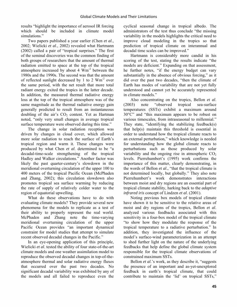
Global Climate Models and Their Limitations
45
results “highlight the importance of aerosol IR forcing which should be included in climate model simulations.”
Two papers published a year earlier (Chen et al., 2002; Wielicki et al., 2002) revealed what Hartmann (2002) called a pair of “tropical surprises.” The first of the seminal discoveries was the common finding of both groups of researchers that the amount of thermal radiation emitted to space at the top of the tropical atmosphere increased by about 4 Wm-2 between the 1980s and the 1990s. The second was that the amount of reflected sunlight decreased by 1 to 2 Wm-2 over the same period, with the net result that more total radiant energy exited the tropics in the latter decade. In addition, the measured thermal radiative energy loss at the top of the tropical atmosphere was of the same magnitude as the thermal radiative energy gain generally predicted to result from an instantaneous doubling of the air’s CO2 content. Yet as Hartman noted, “only very small changes in average tropical surface temperature were observed during this time.”
The change in solar radiation reception was driven by changes in cloud cover, which allowed more solar radiation to reach the surface of Earth’s tropical region and warm it. These changes were produced by what Chen et al. determined to be “a decadal-time-scale strengthening of the tropical Hadley and Walker circulations.” Another factor was likely the past quarter-century’s slowdown in the meridional overturning circulation of the upper 100 to 400 meters of the tropical Pacific Ocean (McPhaden and Zhang, 2002); this circulation slowdown also promotes tropical sea surface warming by reducing the rate of supply of relatively colder water to the region of equatorial upwelling.
What do these observations have to do with evaluating climate models? They provide several new phenomena for the models to replicate as a test of their ability to properly represent the real world. McPhaden and Zhang note the time-varying meridional overturning circulation of the upper Pacific Ocean provides “an important dynamical constraint for model studies that attempt to simulate recent observed decadal changes in the Pacific.”
In an eye-opening application of this principle, Wielicki et al. tested the ability of four state-of-the-art climate models and one weather assimilation model to reproduce the observed decadal changes in top-of-the-atmosphere thermal and solar radiative energy fluxes that occurred over the past two decades. No significant decadal variability was exhibited by any of the models and all failed to reproduce even the
cyclical seasonal change in tropical albedo. The administrators of the test thus conclude “the missing variability in the models highlights the critical need to improve cloud modeling in the tropics so that prediction of tropical climate on interannual and decadal time scales can be improved.”
Hartmann is considerably more candid in his scoring of the test, stating the results indicate “the models are deficient.” Expanding on that assessment, he further notes, “if the energy budget can vary substantially in the absence of obvious forcing,” as it did over the past two decades, “then the climate of Earth has modes of variability that are not yet fully understood and cannot yet be accurately represented in climate models.”
Also concentrating on the tropics, Bellon et al. (2003) note “observed tropical sea-surface temperatures (SSTs) exhibit a maximum around 30°C” and “this maximum appears to be robust on various timescales, from intraseasonal to millennial.” They state, “identifying the stabilizing feedback(s) that help(s) maintain this threshold is essential in order to understand how the tropical climate reacts to an external perturbation,” which knowledge is needed for understanding how the global climate reacts to perturbations such as those produced by solar variability and the ongoing rise in atmospheric CO2 levels. Pierrehumbert’s (1995) work confirms the importance of this matter, clearly demonstrating, in the words of Bellon et al., “that the tropical climate is not determined locally, but globally.” They also note Pierrehumbert’s work demonstrates interactions between moist and dry regions are an essential part of tropical climate stability, harking back to the adaptive infrared iris concept of Lindzen et al. (2001).
Noting previous box models of tropical climate have shown it to be sensitive to the relative areas of moist and dry regions of the tropics, Bellon et al. analyzed various feedbacks associated with this sensitivity in a four-box model of the tropical climate “to show how they modulate the response of the tropical temperature to a radiative perturbation.” In addition, they investigated the influence of the model’s surface-wind parameterization in an attempt to shed further light on the nature of the underlying feedbacks that help define the global climate system responsible for the tropical climate observations of constrained maximum SSTs.
Bellon et al.’s work, as they describe it, “suggests the presence of an important and as-yet-unexplored feedback in earth’s tropical climate, that could contribute to maintain the ‘lid’ on tropical SSTs,”
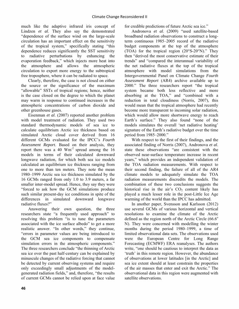
Climate Change Reconsidered II
46
much like the adaptive infrared iris concept of Lindzen et al. They also say the demonstrated “dependence of the surface wind on the large-scale circulation has an important effect on the sensitivity of the tropical system,” specifically stating “this dependence reduces significantly the SST sensitivity to radiative perturbations by enhancing the evaporation feedback,” which injects more heat into the atmosphere and allows the atmospheric circulation to export more energy to the subtropical free troposphere, where it can be radiated to space.
Clearly, therefore, the case is not closed on either the source or the significance of the maximum “allowable” SSTs of tropical regions; hence, neither is the case closed on the degree to which the planet may warm in response to continued increases in the atmospheric concentrations of carbon dioxide and other greenhouse gases.
Eisenman et al. (2007) reported another problem with model treatment of radiation. They used two standard thermodynamic models of sea ice to calculate equilibrium Arctic ice thickness based on simulated Arctic cloud cover derived from 16 different GCMs evaluated for the IPCC’s Fourth Assessment Report. Based on their analysis, they report there was a 40 Wm-2 spread among the 16 models in terms of their calculated downward longwave radiation, for which both sea ice models calculated an equilibrium ice thickness ranging from one to more than ten meters. They note the mean 1980–1999 Arctic sea ice thickness simulated by the 16 GCMs ranged from only 1.0 to 3.9 meters, a far smaller inter-model spread. Hence, they say they were “forced to ask how the GCM simulations produce such similar present-day ice conditions in spite of the differences in simulated downward longwave radiative fluxes?”
Answering their own question, the three researchers state “a frequently used approach” to resolving this problem “is to tune the parameters associated with the ice surface albedo” to get a more realistic answer. “In other words,” they continue, “errors in parameter values are being introduced to the GCM sea ice components to compensate simulation errors in the atmospheric components.” The three researchers conclude “the thinning of Arctic sea ice over the past half-century can be explained by minuscule changes of the radiative forcing that cannot be detected by current observing systems and require only exceedingly small adjustments of the model-generated radiation fields,” and, therefore, “the results of current GCMs cannot be relied upon at face value
for credible predictions of future Arctic sea ice.” Andronova et al. (2009) “used satellite-based
broadband radiation observations to construct a long-term continuous 1985–2005 record of the radiative budget components at the top of the atmosphere (TOA) for the tropical region (20°S-20°N).” They then “derived the most conservative estimate of their trends” and “compared the interannual variability of the net radiative fluxes at the top of the tropical atmosphere with model simulations from the Intergovernmental Panel on Climate Change Fourth Assessment Report (AR4) archive available up to 2000.” The three researchers report “the tropical system became both less reflective and more absorbing at the TOA,” and “combined with a reduction in total cloudiness (Norris, 2007), this would mean that the tropical atmosphere had recently become more transparent to incoming solar radiation, which would allow more shortwave energy to reach Earth’s surface.” They also found “none of the models simulates the overall ‘net radiative heating’ signature of the Earth’s radiative budget over the time period from 1985–2000.”
With respect to the first of their findings, and the associated finding of Norris (2007), Andronova et al. state these observations “are consistent with the observed near-surface temperature increase in recent years,” which provides an independent validation of the TOA radiation measurements. With respect to their second finding, the failure of all of the AR4 climate models to adequately simulate the TOA radiation measurements discredits the models. The combination of these two conclusions suggests the historical rise in the air’s CO2 content likely has played a much lesser role in the post-Little Ice Age warming of the world than the IPCC has admitted.
In another paper, Svensson and Karlsson (2012) use several GCMs of various horizontal and vertical resolutions to examine the climate of the Arctic defined as the region north of the Arctic Circle (66.6o N). They were concerned with modelling the winter months during the period 1980–1999, a time of limited observational data sets. The observations used were the European Centre for Long Range Forecasting (ECMWF) ERA reanalyses. The authors write, “one should be cautious to interpret the data as ‘truth’ in this remote region. However, the abundance of observations at lower latitudes [in the Arctic] and sea ice extent should at least constrain the properties of the air masses that enter and exit the Arctic.” The observational data in this region were augmented with satellite observations.
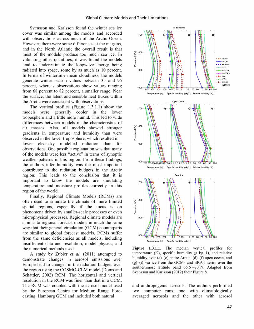
Global Climate Models and Their Limitations
47
Svensson and Karlsson found the winter sea ice cover was similar among the models and accorded with observations across much of the Arctic Ocean. However, there were some differences at the margins, and in the North Atlantic the overall result is that most of the models produce too much sea ice. In validating other quantities, it was found the models tend to underestimate the longwave energy being radiated into space, some by as much as 10 percent. In terms of wintertime mean cloudiness, the models generate winter season values between 35 and 95 percent, whereas observations show values ranging from 68 percent to 82 percent, a smaller range. Near the surface, the latent and sensible heat fluxes within the Arctic were consistent with observations.
The vertical profiles (Figure 1.3.1.1) show the models were generally cooler in the lower troposphere and a little more humid. This led to wide differences between models in the characteristics of air masses. Also, all models showed stronger gradients in temperature and humidity than were observed in the lower troposphere, which resulted in lower clear-sky modelled radiation than for observations. One possible explanation was that many of the models were less “active” in terms of synoptic weather patterns in this region. From these findings, the authors infer humidity was the most important contributor to the radiation budgets in the Arctic region. This leads to the conclusion that it is important to know the models are simulating temperature and moisture profiles correctly in this region of the world.
Finally, Regional Climate Models (RCMs) are often used to simulate the climate of more limited spatial regions, especially if the focus is on phenomena driven by smaller-scale processes or even microphysical processes. Regional climate models are similar to regional forecast models in much the same way that their general circulation (GCM) counterparts are similar to global forecast models. RCMs suffer from the same deficiencies as all models, including insufficient data and resolution, model physics, and the numerical methods used.
A study by Zubler et al. (2011) attempted to demonstrate changes in aerosol emissions over Europe lead to changes in the radiation budgets over the region using the COSMO-CLM model (Doms and Schättler, 2002) RCM. The horizontal and vertical resolution in the RCM was finer than that in a GCM. The RCM was coupled with the aerosol model used by the European Centre for Medium Range Fore-casting, Hamburg GCM and included both natural
and anthropogenic aerosols. The authors performed two computer runs, one with climatologically averaged aerosols and the other with aerosol
Figure 1.3.1.1. The median vertical profiles for temperature (K), specific humidity (g kg−1), and relative humidity over (a)–(c) entire Arctic, (d)–(f) open ocean, and (g)–(i) sea ice from the GCMs and ERA-Interim over the southernmost latitude band 66.6°–70°N. Adapted from Svensson and Karlsson (2012) their Figure 8.
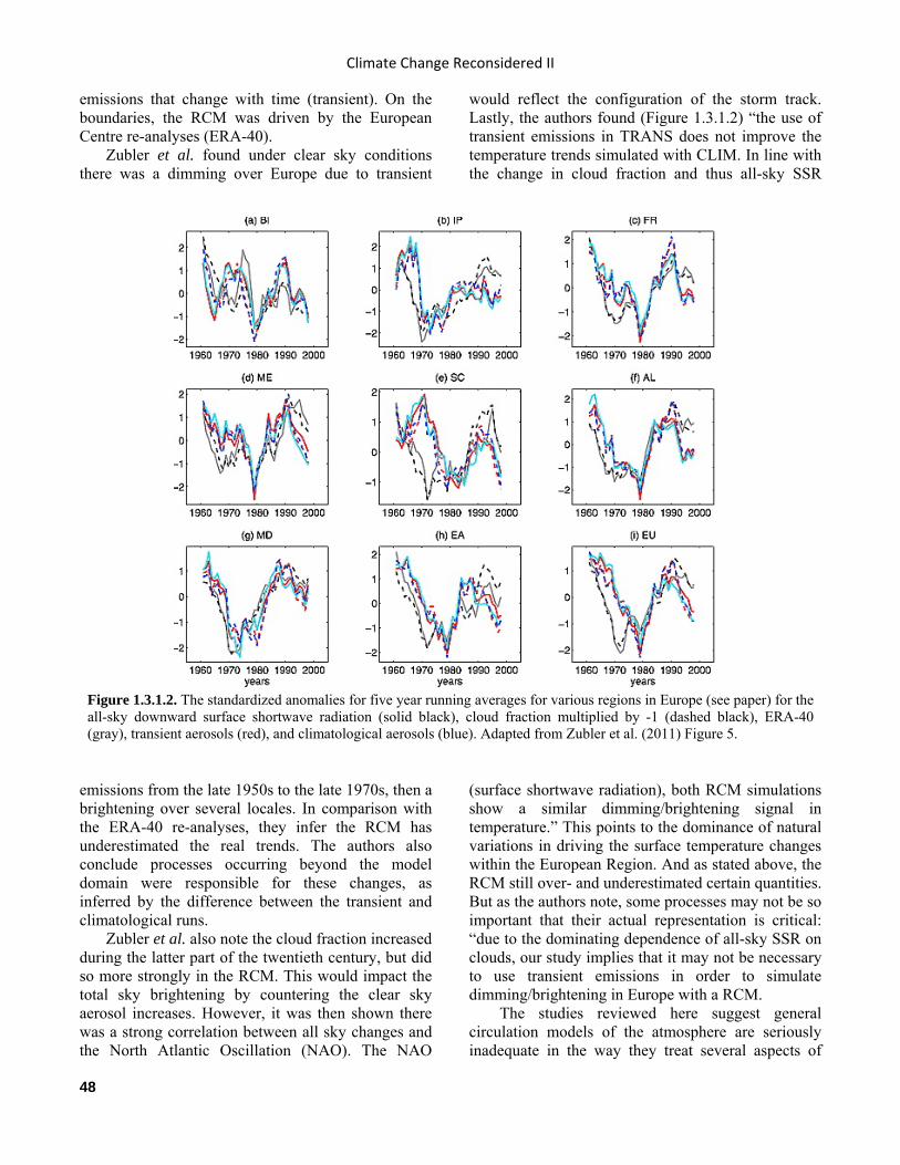
Climate Change Reconsidered II
48
emissions that change with time (transient). On the boundaries, the RCM was driven by the European Centre re-analyses (ERA-40).
Zubler et al. found under clear sky conditions there was a dimming over Europe due to transient
emissions from the late 1950s to the late 1970s, then a brightening over several locales. In comparison with the ERA-40 re-analyses, they infer the RCM has underestimated the real trends. The authors also conclude processes occurring beyond the model domain were responsible for these changes, as inferred by the difference between the transient and climatological runs.
Zubler et al. also note the cloud fraction increased during the latter part of the twentieth century, but did so more strongly in the RCM. This would impact the total sky brightening by countering the clear sky aerosol increases. However, it was then shown there was a strong correlation between all sky changes and the North Atlantic Oscillation (NAO). The NAO
would reflect the configuration of the storm track. Lastly, the authors found (Figure 1.3.1.2) “the use of transient emissions in TRANS does not improve the temperature trends simulated with CLIM. In line with the change in cloud fraction and thus all-sky SSR
(surface shortwave radiation), both RCM simulations show a similar dimming/brightening signal in temperature.” This points to the dominance of natural variations in driving the surface temperature changes within the European Region. And as stated above, the RCM still over- and underestimated certain quantities. But as the authors note, some processes may not be so important that their actual representation is critical: “due to the dominating dependence of all-sky SSR on clouds, our study implies that it may not be necessary to use transient emissions in order to simulate dimming/brightening in Europe with a RCM.
The studies reviewed here suggest general circulation models of the atmosphere are seriously inadequate in the way they treat several aspects of
Figure 1.3.1.2. The standardized anomalies for five year running averages for various regions in Europe (see paper) for the all-sky downward surface shortwave radiation (solid black), cloud fraction multiplied by -1 (dashed black), ERA-40 (gray), transient aerosols (red), and climatological aerosols (blue). Adapted from Zubler et al. (2011) Figure 5.

Global Climate Models and Their Limitations
49
Earth’s radiative energy balance—and fail entirely to address some pertinent phenomena.
References Andronova, N., Penner, J.E., and Wong, T. 2009. Observed and modeled evolution of the tropical mean radiation budget at the top of the atmosphere since 1985. Journal of Geophysical Research 114: 10.1029/2008JD011560.
Bellon, G., Le Treut, H., and Ghil, M. 2003. Large-scale and evaporation-wind feedbacks in a box model of the tropical climate. Geophysical Research Letters 30: 10.1029/2003GL017895.
Chambers, F.M., Ogle, M.I., and Blackford, J.J. 1999. Palaeoenvironmental evidence for solar forcing of Holocene climate: linkages to solar science. Progress in Physical Geography 23: 181–204.
Chen, J., Carlson, B.E., and Del Genio, A.D. 2002. Evidence for strengthening of the tropical general circulation in the 1990s. Science 295: 838–841.
Doms, G. and Schättler, U. 2002. A description of the nonhydrostatic regional model LM, Part I: Dynamics and numerics, technical report, Dtsch. Wetterdienst, Offenbach am Main, Germany.
Eisenman, I., Untersteiner, N., and Wettlaufer, J.S. 2007. On the reliability of simulated Arctic sea ice in global climate models. Geophysical Research Letters 34: 10.1029/2007GL029914.
Ghan, S.J., Easter, R.C., Chapman, E.G., Abdul-Razzak, H., Zhang, Y., Leung, L.R., Laulainen, N.S., Saylor, R.D., and Zaveri, R.A. 2001. A physically based estimate of radiative forcing by anthropogenic sulfate aerosol. Journal of Geophysical Research 106: 5279–5293.
Harries, J.E. 2000. Physics of the earth’s radiative energy balance. Contemporary Physics 41: 309–322.
Hartmann, D.L. 2002. Tropical surprises. Science 295: 811–812.
Jacobson, M.Z. 2001. Global direct radiative forcing due to multicomponent anthropogenic and natural aerosols. Journal of Geophysical Research 106: 1551–1568.
Lindzen, R.S., Chou, M.-D., and Hou, A.Y. 2001. Does the earth have an adaptive infrared iris? Bulletin of the American Meteorological Society 82: 417–432.
McPhaden, M.J. and Zhang, D. 2002. Slowdown of the meridional overturning circulation in the upper Pacific Ocean. Nature 415: 603–608.
Norris, J.R. 2007. Observed interdecadal changes in cloudiness: Real or spurious? In: Broennimann, S. et al.
(Eds.) Climate Variability and Extremes During the Past 100 Years. Springer, New York, NY, USA, pp. 169–178.
Pierrehumbert, R.T. 1995. Thermostats, radiator fins, and the local runaway greenhouse. Journal of the Atmospheric Sciences 52: 1784–1806.
Sokolik, I.N., Toon, O.B., and Bergstrom, R.W. 1998. Modeling the radiative characteristics of airborne mineral aerosols at infrared wavelengths. Journal of Geophysical Research 103: 8813–8826.
Svensson, G. and J. Karlsson, 2012: On the arctic wintertime climate in global climate models. Journal of Climate 24: 5757-5771. DOI:10.
Tegen, I., Lacis, A.A., and Fung, I. 1996. The influence on climate forcing of mineral aerosols from disturbed soils. Nature 380: 419–422.
Vogelmann, A.M., Flatau, P.J., Szczodrak, M., Markowicz, K.M., and Minnett, P.J. 2003. Observations of large aerosol infrared forcing at the surface. Geophysical Research Letters 30: 10.1029/2002GL016829.
Wielicki, B.A., Wong, T., Allan, R.P., Slingo, A., Kiehl, J.T., Soden, B.J., Gordon, C.T., Miller, A.J., Yang, S.-K., Randall, D.A., Robertson, F., Susskind, J., and Jacobowitz, H. 2002. Evidence for large decadal variability in the tropical mean radiative energy budget. Science 295: 841–844.
Wild, M. 1999. Discrepancies between model-calculated and observed shortwave atmospheric absorption in areas with high aerosol loadings. Journal of Geophysical Research 104: 27,361–27,371.
Wild, M. and Ohmura, A. 1999. The role of clouds and the cloud-free atmosphere in the problem of underestimated absorption of solar radiation in GCM atmospheres. Physics and Chemistry of the Earth 24B: 261–268.
Zender, C.S. 1999. Global climatology of abundance and solar absorption of oxygen collision complexes. Journal of Geophysical Research 104: 24,471–24,484.
Zubler, E.M, Folini, D., Lohmann, U., Lüthi, D., Schär, C., and M. Wild, 2011: Simulation of dimming and brightening in Europe from 1958 to 2001 using a regional climate model. Journal of Geophysical Research 116: D18205, doi:10.1029/2010JD015396.
1.3.2 Water Vapor “Water vapor feedback in climate models is large and positive,” note Paltridge et al. (2009), and “the various model representations and parameterizations of convection, turbulent transfer, and deposition of latent heat generally maintain a more-or-less constant

Climate Change Reconsidered II
50
relative humidity (i.e., an increasing specific humidity q) at all levels in the troposphere as the planet warms.” This “increasing q amplifies the response of surface temperature to increasing CO2 by a factor or 2 or more,” they write. They also note the behavior of water vapor in the middle and upper levels of the troposphere dominates overall water-vapor feedback. It is at these levels where long-term measurements of the trends in water vapor concentration are least reliable.
Consequently, knowledge of how q (particularly the q of the upper levels of the troposphere) responds to atmospheric warming is of paramount importance to the task of correctly predicting the water vapor feedback and how air temperatures respond to increasing CO2 concentrations. Paltridge et al. explore this important subject by determining trends in relative and specific humidity at various levels in the atmosphere based on reanalysis data of the National Centers for Environmental Prediction (NCEP) for the period 1973–2007. The three researchers report “the face-value 35-year trend in zonal-average annual-average specific humidity q is significantly negative at all altitudes above 850 hPa (roughly the top of the convective boundary layer) in the tropics and southern midlatitudes and at altitudes above 600 hPa in the northern midlatitudes.” They conclude “negative trends in q as found in the NCEP data would imply that long-term water vapor feedback is negative—that it would reduce rather than amplify the response of the climate system to external forcing such as that from increasing atmospheric CO2.”
As discussed by Boehmer (2012), there is a continuing argument on this topic that boils down to two main issues. First, there is the question as to whether in situ balloon measurements, which suggest a negative long-term trend in upper-level q and hence a negative water vapor feedback, or remote sensing satellite measurements, which suggest the opposite, are correct in their measurements of q. The second question concerns whether short-term correlations between upper-level q and surface temperature can be extrapolated to deduce the existence of such a correlation over longer time scales.
Boehmer’s work is critical, as the assumption that humidity will remain constant and act as an amplifier is based largely on models, which is circular reasoning. If water vapor is not an amplifier but acts as a negative feedback, the case for high climate sensitivity and alarming rates of warming is based entirely on models and not real-world data.
References Boehmer, S. 2012. Science debates must continue. Energy and the Environment 23: 1483–1487.
Paltridge, G., Arking, A., and Pook, M. 2009. Trends in middle- and upper-level tropospheric humidity from NCEP reanalysis data. Theoretical and Applied Climatology 98: 351–359.
1.3.3 Aerosols 1.3.3.1 Aerosols Aerosols, whether natural or anthropogenic, can affect the weather and climate in many ways. The most obvious is by increasing the planetary albedo, which leads to a surface cooling. Aerosols also can warm the middle and upper troposphere if they absorb sunlight, possibly increasing atmospheric stability and inhibiting cloud formation. They can have indirect effects as well, by changing the nature of clouds and the formation of precipitation. And like clouds, they can only be parameterized in weather and climate models. The inadequate treatment of aerosols by GCMs represents a major limitation in the models’ reliability.
Mishchenko et al. (2009) state “because of the global nature of aerosol climate forcings, satellite observations have been and will be an indispensable source of information about aerosol characteristics for use in various assessments of climate and climate change,” and they note “there have been parallel claims of unprecedented accuracy of aerosol retrievals with the moderate-resolution imaging spectroradiometer (MODIS) and multi-angle imaging spectroradiometer (MISR).”
If both aerosol retrieval systems are as good as they have been claimed to be, they should agree on a pixel by pixel basis as well as globally. Consequently, and noting “both instruments have been flown for many years on the same Terra platform, which provides a unique opportunity to compare fully collocated pixel-level MODIS and MISR aerosol retrievals directly,” Mishchenko et al. decided to see how they compare in this regard by analyzing eight years of such data.
The six scientists from NASA’s Goddard Institute for Space Studies report finding what they describe as “unexpected significant disagreements at the pixel level as well as between long-term and spatially averaged aerosol properties.” In fact, they note, “the only point on which both datasets seem to fully agree
Global Climate Models and Their Limitations
51
is that there may have been a weak increasing tendency in the globally averaged aerosol optical thickness (AOT) over the land and no long-term AOT tendency over the oceans.” The NASA scientists state their conclusion quite succinctly: “[O]ur new results suggest that the current knowledge of the global distribution of the AOT and, especially, aerosol microphysical characteristics remains unsatisfactory.” And since this knowledge is indispensable “for use in various assessments of climate and climate change,” it would appear current assessments of greenhouse-gas forcing of climate made by the best models in use today may be of very little worth in describing the real world of nature.
In a contemporaneous study, Haerter et al. (2009) note future projections of climate “have been—for a given climate model—derived using a ‘standard’ set of cloud parameters that produce realistic present-day climate.” However, they add, “there may exist another set of parameters that produces a similar present-day climate but is more appropriate for the description of climate change” and, “due to the high sensitivity of aerosol forcing (F) to cloud parameters, the climate projection with this set of parameters could be notably different from that obtained from the standard set of parameters, even though the present-day climate is reproduced adequately.” This state of affairs suggests replication of the present-day climate is no assurance that a climate model will accurately portray Earth’s climate at some future time. It is also noted this study did not examine first principles, but rather the treatment of radiational forcing, which must be parameterized.
To get a better idea of the magnitude of uncertainty associated with this conundrum, Haerter et al. used the ECHAM5 atmospheric general circulation model, which includes parameterizations of direct and first indirect aerosol effects, to determine what degree of variability in F results from reasonable uncertainties associated with seven different cloud parameters: the entrainment rate (the rate at which environmental air and cloud air mix) for shallow convection, the entrainment rate for penetrative convection, the cloud mass flux above the non-buoyancy level, the correction to asymmetry parameter for ice clouds, the inhomogeneity parameter for liquid clouds, the inhomogeneity parameter for ice clouds, and the conversion efficiency from cloud water to precipitation.
Upon completion of their analyses, the four researchers report “the uncertainty due to a single one of these parameters can be as large as 0.5 W/m2” and
“the uncertainty due to combinations of these parameters can reach more than 1 W/m2.” As for the significance of their findings, they write, “these numbers should be compared with the sulfate aerosol forcing of -1.9 W/m2 for the year 2000, obtained using the default values of the parameters.”
The mean sulfate aerosol forcing component of Earth’s top-of-the-atmosphere radiative budget is thus apparently not known to within anything better than ± 50 percent. In addition, Haerter et al. (2009) note structural uncertainties, such as “uncertainties in aerosol sources, representation of aerosols in models, parameterizations that relate aerosols and cloud droplets to simulate the indirect aerosol effect, and in cloud schemes” lead to an overall uncertainty in F of approximately ± 43 percent, as noted by IPCC. In reality, therefore, the current atmosphere’s aerosol radiative forcing is probably not known to anything better than ± 100%, which does not engender confidence in the ability to simulate Earth’s climate very far into the future.
In another study, Booth et al. (2012) note “a number of studies have provided evidence that aerosols can influence long-term changes in sea surface temperatures,” citing Mann and Emanuel (2006) and Evan et al. (2009), but “climate models have so far failed to reproduce these interactions,” citing Knight (2009) and Ting et al. (2009). They consequently note, as they phrase it, “the role of aerosols in decadal variability remains unclear.”
Booth et al. used the Hadley Centre Global Environmental Model version 2 (HadGEM2-ES)—a next-generation Climate Model Intercomparison Project phase 5 (CMIP5) model—to determine whether older CMIP3 models “contained the complexity necessary to represent a forced Atlantic Multidecadal Oscillation.” The five researchers were thus able to demonstrate that “aerosol emissions and periods of volcanic activity explain 76% of the simulated multidecadal variance in detrended 1860–2005 North Atlantic sea surface temperatures,” and “after 1950, simulated variability is within observational estimates,” while their estimates for 1910–1940 “capture twice the warming of previous generation models,” although they still “do not explain the entire observed trend.” Put another way, they state that “mechanistically, we find that inclusion of aerosol-cloud microphysical effects, which were included in few previous multimodel ensembles, dominates the magnitude (80%) and the spatial pattern of the total surface aerosol forcing in the North Atlantic.”
Climate Change Reconsidered II
52
Booth et al. conclude their paper by noting, “one of the reasons why the role of aerosols in driving multidecadal variability has not previously been identified” is that “although all the CMIP3 models represented the direct effect of aerosols on shortwave radiation, most omitted or only partly represented the indirect aerosol effects,” citing Chang et al. (2011). They conclude, “we need to reassess the current attribution to natural ocean variability of a number of prominent past climate impacts linked to North Atlantic sea surface temperatures.”
Similarly, it may be that climatologists need to reassess the attribution of the post-Little Ice Age warming of the world to anthropogenic CO2 emissions, to account for the possible warming effects of still other as-yet-unappreciated phenomena that are either “omitted or only partly represented” in current state-of-the-art climate models. Some of these phenomena may be associated with things transpiring on (or within) the Sun; other phenomena that may thwart or significantly reduce the warming effect of rising atmospheric CO2 concentrations may be associated with a variety of biological responses of both marine and terrestrial vegetation to atmospheric CO2 enrichment, as well as to warming itself. References Booth, B.B.B., Dunstone, N.J., Halloran, P.R., Andrews, T., and Bellouin, N. 2012. Aerosols implicated as a prime driver of twentieth-century North Atlantic climate variability. Nature 484: 228–232.
Chang, C.Y., Chiang, J.C.H., Wehner, M.F. Friedman, A., and Ruedy, R. 2011. Sulfate aerosol control of tropical Atlantic climate over the 20th century. Journal of Climate 24: 2540–2555.
Evan, A.T., Vimont, D.J., Heidinger, A.K., Kossin, J.P., and Bennartz, R. 2009. The role of aerosols in the evolution of tropical North Atlantic Ocean temperature anomalies. Science 324: 778–781.
Haerter, J.O., Roeckner, E., Tomassini, L., and von Storch, J.-S. 2009. Parametric uncertainty effects on aerosol radiative forcing. Geophysical Research Letters 36: 10.1029/2009GL039050.
Knight, J.R. 2009. The Atlantic Multidecadal Oscillation inferred from the forced climate response in coupled general circulation models. Journal of Climate 22: 1610–1625.
Mann, M.E. and Emanuel, K.A. 2006. Atlantic hurricane trends linked to climate change. EOS, Transactions, American Geophysical Union 87: 233–244.
Mishchenko, M.I., Geogdzhayev, I.V., Liu, L., Lacis, A.A., Cairns, B., and Travis, L.D. 2009. Toward unified satellite climatology of aerosol properties: What do fully compatible MODIS and MISR aerosol pixels tell us? Journal of Quantitative Spectroscopy & Radiative Transfer 110: 402–408.
Ting, M., Kushnir, Y., Seager, R., and Li, C. 2009. Forced and internal twentieth-century SST trends in the North Atlantic. Journal of Climate 22: 1469–1481.
1.3.3.2 Aerosol Nuclei Many physical processes must be approximated in GCMs using separate calculations at the grid scale, called parameterizations. In many cases this involves averaging the effect of subgrid scale processes. These processes include the existence and formation of clouds and also relate to the presence of aerosols or particulates in the air that are not considered to be part of the basic makeup the atmosphere but which strongly affect radiation fluxes. Aerosols are important because they can affect energy exchanges in the atmosphere and serve as condensation nuclei for cloud formation. Clouds have an impact on Earth’s energy budget through their ability to reflect and scatter light and to absorb and emit infrared radiation. Also, cloud properties such as droplet size and concentration can influence how effectively clouds contribute to the planet’s albedo.
Roesler and Penner (2010) used a microsphysical model to explore the effects of the chemical composition and size of aerosols on the concentration of cloud droplets over the United States. Using aerosol composition measurements from 1988 to 2004, the authors found aerosols influenced the size and concentration of the cloud droplets that ultimately formed in their experiments.
They also included tests varying the strength of the atmospheric vertical motions lifting air parcels, which are initially saturated, over a distance of about 300 meters in order to induce cloud formation. They found that as vertical motion increased in strength within their model, the number of cloud droplets increased. They also found that larger aerosols, though fewer in number, were more soluble as they formed cloud droplets. Smaller aerosols were more numerous but less soluble. Thus, the larger aerosols were found to be better at producing cloud droplets. The size of the aerosols depended on their chemical composition, which varied by region across the United States and by season. They found the concentrations of droplets were largest in the eastern
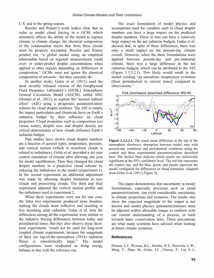
Global Climate Models and Their Limitations
53
U.S. and in the spring season. Roesler and Penner’s work makes clear that in
order to model cloud forcing in a GCM, which ultimately affects the ability of the model to capture climate or climate change, the chemical composition of the condensation nuclei that form these clouds must be properly accounted. Roesler and Penner pointed out, “a global model using an empirical relationship based on regional measurements could over- or under-predict droplet concentrations when applied to other regions depending on differences in composition.” GCMs must not ignore the chemical composition of aerosols—but they currently do.
In another study, Golaz et al. (2011) used the most recently released version of the Geophysical Fluid Dynamics Laboratory’s (GFDL) Atmospheric General Circulation Model (AGCM), called AM3 (Donner et al., 2011), to explore the “aerosol indirect effect” (AIE) using a prognostic parameterization scheme for cloud droplet numbers. The AIE is simply the impact particulates and chemicals have on Earth’s radiation budget by their influence on cloud properties. Cloud properties such as composition (ice versus water), droplet size, and droplet density are critical determinants of how clouds influence Earth’s radiation budget.
Past studies have shown cloud droplet numbers are a function of aerosol types, temperature, pressure, and vertical motion (which in stratiform clouds is related to turbulence). Golaz et al. provided a six-year control simulation of climate after allowing one year for model equilibration. Then they changed the cloud droplet numbers in a predictive cloud scheme by reducing the turbulence in the model (experiment 1). In the second experiment an additional adjustment was made by allowing droplet formation in new clouds and preexisting clouds. The third and final experiment adjusted the vertical motion profile and the turbulence used in experiment 2.
When these experiments were run for one year, the latter two experiments produced more droplets, making the clouds more reflective and resulting in less incoming solar radiation. Golaz et al. note the differences among all the experiments were similar to the radiative forcing differences between today and preindustrial times. But they also observe these short-term experiments “could not be used for long-term coupled climate experiments, because the magnitude of their net top-of-the-atmosphere (TOA) radiation fluxes is unrealistically large.” The model configurations were readjusted to bring energy balance in line with the reference run.
The exact formulation of model physics and assumptions used for variables such as cloud droplet numbers can have a large impact on the predicted droplet numbers. These in turn can have a relatively large impact on the net radiation budgets. Golaz et al. showed that, in spite of these differences, there was only a small impact on the present-day climate overall. However, when the three formulations were applied between present-day and pre-industrial climate, there was a large difference in the net radiation budgets, which can be attributed to the AEI (Figure 1.3.3.2.1). This likely would result in the model yielding “an unrealistic temperature evolution [from preindustrial to current times] compared to observations.”
This paper demonstrates that uncertainty in model formulations, especially processes such as cloud parameterizations, can yield considerable uncertainty in climate projections and scenarios. The results also show the expected magnitude of the output is not known and model physics (parameterizations) must be adjusted within allowable ranges to conform with our current understanding of a process, or back towards basic conservation laws. These precautions are what many scientists have advised when looking at future climate scenarios. References Donner, L.J., Wyman, B.L., Hemler, R.S., Horowitz, L.W., Ming, Y., Zhao, M., Golaz, J.C., Ginoux, P., Lin, S.-J.,
Figure 1.3.3.2.1. The zonal mean difference in the top of the atmosphere shortwave absorption between model runs with present-day conditions and preindustrial conditions using the control and three experimental parameterizations described here. The thicker lines indicate which results are statistically significant at the 95% confidence level. The red line represents the control run, and the blue, green, and purple represent the model configured for differences in cloud formation. Adapted from Golaz et al. (2011) Figure 5a.
Climate Change Reconsidered II
54
Schwarzkopf, M.D., Austin, J., Alaka, G., Cooke, W.F., Delworth, T.L., Freidenreich, S.M., Gordon, C.T., Griffies, S.M., Held, I.M., Hurlin, W.J., Klein, S.A., Knutson, T.R., Langenhorst, A.R., Lee, H.-C., Lin, Y., Magi, B.I., Malyshev, S.L., Milly, P.C.D., Naik, V., Nath, M.J., Pincus, R., Ploshay, J.J., Ramaswamy, V., Seman, C.J., Shevliakova, E., Sirutis, J.J., Stern, W.F., Stouffer, R.J., Wilson, R.J., Winton, M., Wittenberg, A.T., and Zenga, F. 2011. The dynamical core, physical parameterizations, and basic simulations characteristics of the atmospheric component of the GFDL Global Coupled Model CM3. Journal of Climate 24: 3484–3519.
Golaz, J.-C., Salzmann, M., Donner, L.J., Horowitz, L.W., Ming, Y., and Zhao, M. 2011. Sensitivity of the aerosol indirect effect to subgrid variability in the cloud parameterization of the GFDL atmosphere general circulation model AM3. Journal of Climate 24: 3145–3160.
Roesler, E.L. and Penner, J.E. 2010. Can global models ignore the chemical composition of aerosols? Geophysical Research Letters 37: L24809, doi:10.1029/2010GL044282.
1.3.3.3 Volcanic Aerosols The effects of volcanic eruptions on climate have been studied and are well-known. Volcanic eruptions eject particulate and aerosol materials into the stratosphere. These aerosols, primarily sulfate type, increase the albedo of the planet, resulting in less incoming solar radiation and a cooling of the lower troposphere and surface. Generally, the greater the eruption, the stronger this effect will be and the longer it will last. Volcanic eruptions whose emissions are confined to the troposphere generally have little effect on climate, as the troposphere is more efficient in scavenging out the relatively large particulates.
Volcanism is an “external” forcing to Earth’s atmosphere and its occurrence is considered to be unpredictable and irregular. However, once the particulate matter and aerosols are injected into the atmosphere, it is possible to project the spread of the material using a GCM. In June 2009, the Sarychev volcano in Russia’s Kamchatka Peninsula erupted explosively for approximately five days. At the time it was the second such eruption within a year. It injected 1.2 teragrams (Tg) of material into the atmosphere to an estimated height of as much as 16 km—nearly 10 miles.
Kravitz et al. (2011) studied measurements of the optical depth of the aerosol sulfates from this eruption and compared these with the projected output from a 20-member ensemble using a GCM, with the goal of
providing suggestions for improving the model’s capabilities. They used the National Aeronautics and Space Administration (NASA) Goddard Institute for Space Studies Model-E, which employs a coupled atmosphere-ocean GCM with fairly coarse resolution in the horizontal (4° by 5° lat/lon) and vertical (23 layers). The model contained levels up to 80 km, necessarily including the stratosphere.
The control model run consisted of a 20-member suite globally from 2007 to 2010. In the experiment, 1.5 Tg of volcanic material was injected into the atmosphere at a point near Sarychev in 2008 of the model year. The observed aerosol measurements came from ground-based LIDARS at six locations around the world as well as satellite-based measurements that profile the aerosol concentration using scattered sunlight (Optical Spectrograph and Infrared Imaging System (OSIRIS)).
The authors found the model did a reasonably good job of spreading the volcanic material around the Northern Hemisphere, but there were some important discrepancies between the model and observations (e.g. Figure 1.3.3.3.1). For example, the model transported the material too quickly into the tropics and too slowly into the high latitudes. The authors speculate this error may indicate a need to improve the model’s depiction of stratospheric circulation. Also, the model tended to remove aerosols too quickly from the atmosphere, especially in the high latitudes, which may have been an indication of model overestimation of particulate size. Note that in Figure 1.3.3.3.1, the modeled peak aerosol values occurred one month earlier than observed and then decreased in concentration too quickly.
The sensitivity of GCMs to aerosol forcing also can be assessed based on volcanic activity. The Pinatubo eruption of 1991 was very large and explosive, injecting a huge amount of sulfate aerosols into the atmosphere. The climate cooled in response, but the climate models cooled much more than the actual atmosphere, showing the models assumed strong radiative forcing (cooling) by sulfate aerosols, a result also noted by Landrum et al. (2013). This is important because one of the key assumptions of the models is that human pollution, particularly in the post-1970 period, strongly dampens out the warming that greenhouse gas emissions otherwise would have caused. For most of the period simulated, however, no data (or only fragmentary data) are available to estimate sulfate aerosol pollution. Furthermore, the forcing by any given level of aerosols is not easily
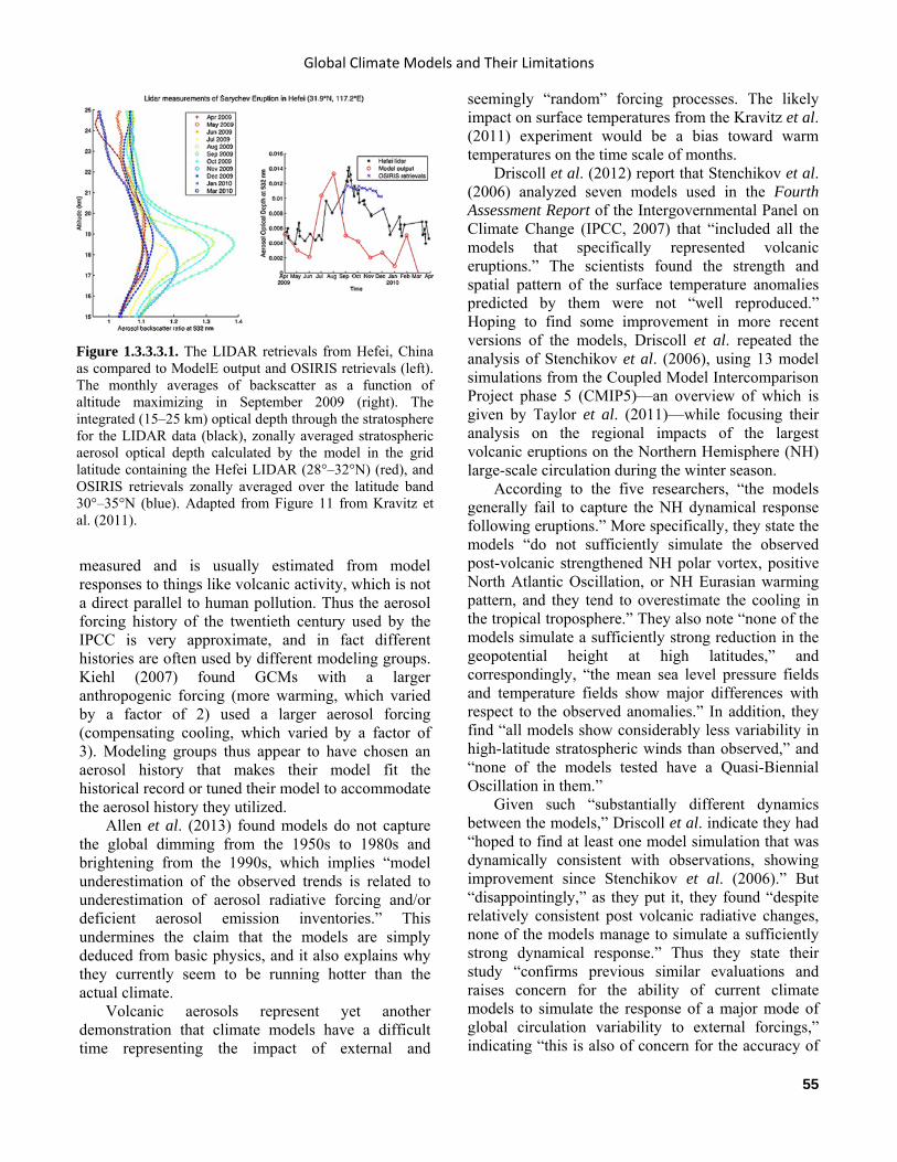
Global Climate Models and Their Limitations
55
measured and is usually estimated from model responses to things like volcanic activity, which is not a direct parallel to human pollution. Thus the aerosol forcing history of the twentieth century used by the IPCC is very approximate, and in fact different histories are often used by different modeling groups. Kiehl (2007) found GCMs with a larger anthropogenic forcing (more warming, which varied by a factor of 2) used a larger aerosol forcing (compensating cooling, which varied by a factor of 3). Modeling groups thus appear to have chosen an aerosol history that makes their model fit the historical record or tuned their model to accommodate the aerosol history they utilized.
Allen et al. (2013) found models do not capture the global dimming from the 1950s to 1980s and brightening from the 1990s, which implies “model underestimation of the observed trends is related to underestimation of aerosol radiative forcing and/or deficient aerosol emission inventories.” This undermines the claim that the models are simply deduced from basic physics, and it also explains why they currently seem to be running hotter than the actual climate.
Volcanic aerosols represent yet another demonstration that climate models have a difficult time representing the impact of external and
seemingly “random” forcing processes. The likely impact on surface temperatures from the Kravitz et al. (2011) experiment would be a bias toward warm temperatures on the time scale of months.
Driscoll et al. (2012) report that Stenchikov et al. (2006) analyzed seven models used in the Fourth Assessment Report of the Intergovernmental Panel on Climate Change (IPCC, 2007) that “included all the models that specifically represented volcanic eruptions.” The scientists found the strength and spatial pattern of the surface temperature anomalies predicted by them were not “well reproduced.” Hoping to find some improvement in more recent versions of the models, Driscoll et al. repeated the analysis of Stenchikov et al. (2006), using 13 model simulations from the Coupled Model Intercomparison Project phase 5 (CMIP5)—an overview of which is given by Taylor et al. (2011)—while focusing their analysis on the regional impacts of the largest volcanic eruptions on the Northern Hemisphere (NH) large-scale circulation during the winter season.
According to the five researchers, “the models generally fail to capture the NH dynamical response following eruptions.” More specifically, they state the models “do not sufficiently simulate the observed post-volcanic strengthened NH polar vortex, positive North Atlantic Oscillation, or NH Eurasian warming pattern, and they tend to overestimate the cooling in the tropical troposphere.” They also note “none of the models simulate a sufficiently strong reduction in the geopotential height at high latitudes,” and correspondingly, “the mean sea level pressure fields and temperature fields show major differences with respect to the observed anomalies.” In addition, they find “all models show considerably less variability in high-latitude stratospheric winds than observed,” and “none of the models tested have a Quasi-Biennial Oscillation in them.”
Given such “substantially different dynamics between the models,” Driscoll et al. indicate they had “hoped to find at least one model simulation that was dynamically consistent with observations, showing improvement since Stenchikov et al. (2006).” But “disappointingly,” as they put it, they found “despite relatively consistent post volcanic radiative changes, none of the models manage to simulate a sufficiently strong dynamical response.” Thus they state their study “confirms previous similar evaluations and raises concern for the ability of current climate models to simulate the response of a major mode of global circulation variability to external forcings,” indicating “this is also of concern for the accuracy of
Figure 1.3.3.3.1. The LIDAR retrievals from Hefei, China as compared to ModelE output and OSIRIS retrievals (left). The monthly averages of backscatter as a function of altitude maximizing in September 2009 (right). The integrated (15–25 km) optical depth through the stratosphere for the LIDAR data (black), zonally averaged stratospheric aerosol optical depth calculated by the model in the grid latitude containing the Hefei LIDAR (28°–32°N) (red), and OSIRIS retrievals zonally averaged over the latitude band 30°–35°N (blue). Adapted from Figure 11 from Kravitz et al. (2011).
Climate Change Reconsidered II
56
geoengineering modeling studies that assess the atmospheric response to stratosphere-injected particles.” References Allen, R.J., Norris, J.R., and Wild, M. 2013. Evaluation of multidecadal variability in CMIP5 surface solar radiation and inferred underestimation of aerosol direct effects over Europe, China, Japan and India. Journal of Geophysical Research 118: 6311–6336.
Driscoll, S., Bozzo, A., Gray, L.J., Robock, A., and Stenchikov, G. 2012. Coupled Model Intercomparison Project 5 (CMIP5) simulations of climate following volcanic eruptions. Journal of Geophysical Research 117: D17105, 10.1029/JD017607.
Kiehl, J.T. 2007. Twentieth century climate model response and climate sensitivity. Geophysical Research Letters 34: L22710, doi:10.1029/2007GL031383.
Kravitz, B., Robock, A., Bourassa, A., Deshler, T., Wu, D., Mattis, I., Finger, F., Hoffmann, A., Ritter, C., Bitar, L., Duck, T.J., and Barnes J.E. 2011. Simulation and observations of stratospheric aerosols from the 2009 Sarychev volcanic eruption. Journal of Geophysical Research-Atmospheres 116: D18211, doi:10.1029/ 2010JD015501.
Landrum, L., Otto-Bliesner, B.L., Wahl, E.R., Conley, A., Lawrence, P.J., Rosenbloom, N., and Teng, H. 2013. Last millennium climate and its variability in CCSM4. Journal of Climate 26: 1085–1111.
Stenchikov, G., Hamilton, K., Stouffer, R.J., Robock, A., Ramaswamy, V., Santer, B., and Graf, H.-F. 2006. Arctic Oscillation response to volcanic eruptions in the IPCC AR4 climate models. Journal of Geophysical Research 111: D07107, doi:10.1029/2005JD006286.
Taylor, K.E., Stouffer, R.J., and Meehl, G.A. 2011. An overview of CMIP5 and the experiment design. Bulletin of the American Meteorological Society 93: 485–498.
1.3.4 Clouds Correctly parameterizing the influence of clouds on climate is an elusive goal the creators of atmospheric GCMs have yet to achieve. One major reason for their lack of success has to do with inadequate model resolution on vertical and horizontal space scales. Lack of resolution forces modelers to parameterize the ensemble large-scale effects of processes that occur on smaller scales than the models are capable of handling. This is particularly true of physical processes such as cloud formation and cloud-radiation
interactions. Several studies suggest older model parameterizations did not succeed in this regard (Groisman et al., 2000), and subsequent studies, as discussed in this section, suggest they still are not succeeding. The lack of success may not be due entirely to inadequate model resolution: If cloud processes have not been adequately and properly quantified, not even the highest resolution will bring success.
Lane et al. (2000) evaluated the sensitivities of the cloud-radiation parameterizations utilized in contemporary GCMs to changes in vertical model resolution, varying the latter from 16 to 60 layers in increments of four and comparing the results to observed values. This effort revealed cloud fraction varied by approximately 10 percent over the range of resolutions tested, which corresponded to about 20 percent of the observed cloud cover fraction. Similarly, outgoing longwave radiation varied by 10 to 20 Wm-2 as model vertical resolution was varied, amounting to approximately 5 to 10 percent of observed values, and incoming solar radiation experienced similar significant variations across the range of resolutions tested. The model results did not converge, even at a resolution of 60 layers.
In an analysis of the multiple roles played by cloud microphysical processes in determining tropical climate, Grabowski (2000) found much the same thing, noting there were serious problems of computer models failing to correctly incorporate cloud microphysics. These observations led him to conclude “it is unlikely that traditional convection parameterizations can be used to address this fundamental question in an effective way.” He also became convinced that “classical convection parameterizations do not include realistic elements of cloud physics and they represent interactions among cloud physics, radiative processes, and surface processes within a very limited scope.” Consequently, he added, “model results must be treated as qualitative rather than quantitative.”
Reaching similar conclusions were Gordon et al. (2000), who determined many GCMs of the late 1990s tended to under-predict the presence of subtropical marine stratocumulus clouds and failed to simulate the seasonal cycle of clouds. These deficiencies are important because these particular clouds exert a major cooling influence on the surface temperatures of the sea below them. In the situation investigated by Gordon and his colleagues, the removal of the low clouds, as occurred in the normal application of their model, led to sea surface
Global Climate Models and Their Limitations
57
temperature increases on the order of 5.5°C. Further condemnation of turn-of-the-century
model treatments of clouds came from Harries (2000), who write our knowledge of high cirrus clouds is very poor and “we could easily have uncertainties of many tens of Wm-2 in our description of the radiative effect of such clouds, and how these properties may change under climate forcing.”
Lindzen et al. (2001) analyzed cloud cover and sea surface temperature (SST) data over a large portion of the Pacific Ocean, finding a strong inverse relationship between upper-level cloud area and mean SST, such that the area of cirrus cloud coverage normalized by a measure of the area of cumulus coverage decreased by about 22 percent for each degree C increase in cloudy region SST. Essentially, as the researchers describe it, “the cloudy-moist region appears to act as an infrared adaptive iris that opens up and closes down the regions free of upper-level clouds, which more effectively permit infrared cooling, in such a manner as to resist changes in tropical surface temperature.” The sensitivity of this negative feedback was calculated by Lindzen et al. to be substantial. They estimate it would “more than cancel all the positive feedbacks in the more sensitive current climate models” being used to predict the consequences of projected increases in atmospheric CO2 concentration.
Lindzen’s conclusions did not go uncontested, and Hartmann and Michelsen (2002) quickly claimed the correlation noted by Lindzen et al. resulted from variations in subtropical clouds not physically connected to deep convection near the equator, and it was thus “unreasonable to interpret these changes as evidence that deep tropical convective anvils contract in response to SST increases.” Fu et al. (2002) also chipped away at the adaptive infrared iris concept, arguing “the contribution of tropical high clouds to the feedback process would be small since the radiative forcing over the tropical high cloud region is near zero and not strongly positive,” while also claiming to show water vapor and low cloud effects were overestimated by Lindzen et al. by at least 60 percent and 33 percent, respectively. As a result, Fu et al. obtained a feedback factor in the range of -0.15 to -0.51, compared to Lindzen et al.’s much larger negative feedback factor of -0.45 to -1.03.
In a contemporaneously published reply to this critique, Chou et al. (2002) state Fu et al.’s approach of specifying longwave emission and cloud albedos “appears to be inappropriate for studying the iris effect.” Since “thin cirrus are widespread in the
tropics and ... low boundary clouds are optically thick, the cloud albedo calculated by [Fu et al.] is too large for cirrus clouds and too small for boundary layer clouds,” they write, so “the near-zero contrast in cloud albedos derived by [Fu et al.] has the effect of underestimating the iris effect.” In the end, Chou et al. agreed Lindzen et al. “may indeed have overestimated the iris effect somewhat, though hardly by as much as that suggested by [Fu et al.].”
Grassl (2000), in a review of the then-current status of the climate-modeling enterprise two years before the infrared iris effect debate emerged, noted changes in many climate-related phenomena, including cloud optical and precipitation properties caused by changes in the spectrum of cloud condensation nuclei, were insufficiently well known to provide useful insights into future conditions. In light of this knowledge gap, he recommended “we must continuously evaluate and improve the GCMs we use,” although he acknowledges contemporary climate model results were already being “used by many decision-makers, including governments.”
Some may consider what is currently known about clouds to be sufficient for predictive purposes, but the host of questions posed by Grassl—for which definitive answers are still lacking—demonstrates this assumption is erroneous. As but a single example, Charlson et al. (1987) describe a negative feedback process that links biologically produced dimethyl sulfide (DMS) in the oceans with climate. (See Chapter 2 of this volume for a more complete discussion of this topic.) This hypothesis holds that the global radiation balance is significantly influenced by the albedo of marine stratus clouds and that the albedo of these clouds is a function of cloud droplet concentration, which is dependent upon the availability of condensation nuclei that have their origin in the flux of DMS from the world’s oceans to the atmosphere.
Acknowledging that the roles played by DMS oxidation products in the context described above are “diverse and complex” and in many instances “not well understood,” Ayers and Gillett (2000) summarized empirical evidence, derived from data collected at Cape Grim, Tasmania, and from reports of other pertinent studies in the peer-reviewed scientific literature, supporting Charlson et al.’s (1987) hypothesis. Ayers and Gillett found the “major links in the feedback chain proposed by Charlson et al. (1987) have a sound physical basis” and there is “compelling observational evidence to suggest that DMS and its atmospheric products participate

Climate Change Reconsidered II
58
significantly in processes of climate regulation and reactive atmospheric chemistry in the remote marine boundary layer of the Southern Hemisphere.”
The empirical evidence analyzed by Ayers and Gillett highlights an important suite of negative feedback processes that act in opposition to model-predicted CO2-induced global warming over the world’s oceans. These processes are not fully incorporated into even the best of the current climate models, nor are analogous phenomena that occur over land included in them, such as those discussed by Idso (1990).
Further to this point, O’Dowd et al. (2004) measured size-resolved physical and chemical properties of aerosols found in northeast Atlantic marine air arriving at the Mace Head Atmospheric Research station on the west coast of Ireland during phytoplanktonic blooms at various times of the year. They found in the winter, when biological activity was at its lowest, the organic fraction of the sub-micrometer aerosol mass was about 15 percent. During the spring through autumn, however, when biological activity was high, “the organic fraction dominates and contributes 63 percent to the sub-micrometer aerosol mass (about 45 percent is water-insoluble and about 18 percent water-soluble),” they write. Based on these findings, they performed model simulations that indicated the marine-derived organic matter “can enhance the cloud droplet concentration by 15 percent to more than 100 percent and is therefore an important component of the aerosol-cloud-climate feedback system involving marine biota.”
O’Dowd et al. (2004) state their findings “completely change the picture of what influences marine cloud condensation nuclei given that water-soluble organic carbon, water-insoluble organic carbon and surface-active properties, all of which influence the cloud condensation nuclei activation potential, are typically not parameterized in current climate models,” or as they note elsewhere in their paper, “an important source of organic matter from the ocean is omitted from current climate-modeling predictions and should be taken into account.”
Another perspective on the cloud-climate conundrum is provided by Randall et al. (2003), who state at the outset of their review of the subject that “the representation of cloud processes in global atmospheric models has been recognized for decades as the source of much of the uncertainty surrounding predictions of climate variability.” They report that “despite the best efforts of [the climate modeling]
community … the problem remains largely unsolved” and note, “at the current rate of progress, cloud parameterization deficiencies will continue to plague us for many more decades into the future.”
Randall et al. declare “clouds are complicated,” highlighting what they call the “appalling complexity” of the cloud parameterization situation. They also state “our understanding of the interactions of the hot towers [of cumulus convection] with the global circulation is still in a fairly primitive state,” and not knowing all that much about what goes up, it’s not surprising we also don’t know much about what comes down, as they report “downdrafts are either not parameterized or crudely parameterized in large-scale models.” It also should be noted Riehl and Malkus (1958), in an analysis of the equatorial trough region, could not achieve closure of their large-scale energy budgets without resorting to significant vertical exchanges by way of the cumulonimbus downdrafts.
With respect to stratiform clouds, the situation is no better, as their parameterizations are described by Randall et al. as “very rough caricatures of reality.” As for interactions between convective and stratiform clouds, during the 1970s and ‘80s, Randall et al. report “cumulus parameterizations were extensively tested against observations without even accounting for the effects of the attendant stratiform clouds.” They reported the concept of detrainment was “somewhat murky” and the conditions that trigger detrainment were “imperfectly understood.” “At this time,” as they put it, “no existing GCM includes a satisfactory parameterization of the effects of mesoscale cloud circulations.”
Randall et al. additionally state “the large-scale effects of microphysics, turbulence, and radiation should be parameterized as closely coupled processes acting in concert,” but they report only a few GCMs have even attempted to do so. Why? Because, as they continue, “the cloud parameterization problem is overwhelmingly complicated” and “cloud parameterization developers,” as they call them, are still “struggling to identify the most important processes on the basis of woefully incomplete observations.” They add, “there is little question why the cloud parameterization problem is taking a long time to solve: It is very, very hard.” The four scientists conclude, “a sober assessment suggests that with current approaches the cloud parameterization problem will not be ‘solved’ in any of our lifetimes.”
To show the basis for this conclusion is robust and cannot be said to rest on the less-than-enthusiastic

Global Climate Models and Their Limitations
59
remarks of a handful of exasperated climate modelers, additional studies on the subject have been published subsequent to Randall et al., any of which could have readily refuted their assessment of the situation if they thought it was appropriate.
Siebesma et al. (2004), for example, report “simulations with nine large-scale models [were] carried out for June/July/August 1998 and the quality of the results [was] assessed along a cross-section in the subtropical and tropical North Pacific ranging from (235°E, 35°N) to (187.5°E, 1°S),” in order to “document the performance quality of state-of-the-art GCMs in modeling the first-order characteristics of subtropical and tropical cloud systems.” The main conclusions of this study, according to the authors are: “(1) almost all models strongly under predicted both cloud cover and cloud amount in the stratocumulus regions while (2) the situation is opposite in the trade-wind region and the tropics where cloud cover and cloud amount are over predicted by most models.” They report “these deficiencies result in an over prediction of the downwelling surface short-wave radiation of typically 60 Wm-2 in the stratocumulus regimes and a similar under prediction of 60 Wm-2 in the trade-wind regions and in the intertropical convergence zone (ITCZ),” and these discrepancies are to be compared with a radiative forcing of only a couple of Wm-2 for a 300 ppm increase in the atmosphere’s CO2 concentration. In addition, they note “similar biases for the short-wave radiation were found at the top of the atmosphere, while discrepancies in the outgoing long-wave radiation are most pronounced in the ITCZ.”
The 17 scientists hailing from nine different countries who comprised Siebesma et al. also found “the representation of clouds in general-circulation models remains one of the most important as yet unresolved issues in atmospheric modeling.” This is partially due, they continue, “to the overwhelming variety of clouds observed in the atmosphere, but even more so due to the large number of physical processes governing cloud formation and evolution as well as the great complexity of their interactions.” Hence, they conclude that through repeated critical evaluations of the type they conducted, “the scientific community will be forced to develop further physically sound parameterizations that ultimately result in models that are capable of simulating our climate system with increasing realism.”
In their effort to assess the status of state-of-the-art climate models in simulating cloud-related processes, Zhang et al. (2005) compared basic cloud
climatologies derived from ten atmospheric GCMs with satellite measurements obtained from the International Satellite Cloud Climatology Project (ISCCP) and the Clouds and Earth’s Radiant Energy System (CERES) program. ISCCP data were available for 1983–2001, and data from the CERES program were available for the winter months of 2001 and 2002 and for the summer months of 2000 and 2001. The purpose of their analysis was twofold: to assess the current status of climate models in simulating clouds so that future progress can be measured more objectively, and to reveal serious deficiencies in the models so as to improve them.
The work of 20 climate modelers involved in this exercise revealed a long list of major model imperfections. First, Zhang et al. report a fourfold difference in high clouds among the models, and that the majority of the models simulated only 30 to 40 percent of the observed middle clouds, with some models simulating less than a quarter of observed middle clouds. For low clouds, they report half the models underestimated them, such that the grand mean of low clouds from all models was only 70 to 80 percent of what was observed. Furthermore, when stratified in optical thickness ranges, the majority of the models simulated optically thick clouds more than twice as frequently as was found to be the case in the satellite observations, and the grand mean of all models simulated about 80 percent of optically intermediate clouds and 60 percent of optically thin clouds. In the case of individual cloud types, the group of researchers note “differences of seasonal amplitudes among the models and satellite measurements can reach several hundred percent.” Zhang et al. (2005) conclude “much more needs to be done to fully understand the physical causes of model cloud biases presented here and to improve the models.”
L’Ecuyer and Stephens (2007) used multi-sensor observations of visible, infrared, and microwave radiance obtained from the Tropical Rainfall Measuring Mission satellite for the period from January 1998 through December 1999 in order to evaluate the sensitivity of atmospheric heating—and the factors that modify it—to changes in east-west sea surface temperature gradients associated with the strong 1998 El Niño event in the tropical Pacific, as expressed by the simulations of nine general circulation models of the atmosphere that were utilized in the IPCC’s most recent Fourth Assessment Report. This protocol, in their words, “provides a natural example of a short-term climate change
Climate Change Reconsidered II
60
scenario in which clouds, precipitation, and regional energy budgets in the east and west Pacific are observed to respond to the eastward migration of warm sea surface temperatures.”
Results indicate “a majority of the models examined do not reproduce the apparent westward transport of energy in the equatorial Pacific during the 1998 El Niño event.” They also found “the inter-model variability in the responses of precipitation, total heating, and vertical motion is often larger than the intrinsic ENSO signal itself, implying an inherent lack of predictive capability in the ensemble with regard to the response of the mean zonal atmospheric circulation in the tropical Pacific to ENSO.” In addition, they report “many models also misrepresent the radiative impacts of clouds in both regions [the east and west Pacific], implying errors in total cloudiness, cloud thickness, and the relative frequency of occurrence of high and low clouds.” As a result of these much-less-than-adequate findings, the two researchers from Colorado State University’s Department of Atmospheric Science conclude “deficiencies remain in the representation of relationships between radiation, clouds, and precipitation in current climate models,” and these deficiencies “cannot be ignored when interpreting their predictions of future climate.”
In a contemporaneous publication, this one in the Journal of the Atmospheric Sciences, Zhou et al. (2007) state “clouds and precipitation play key roles in linking the Earth’s energy cycle and water cycles,” noting “the sensitivity of deep convective cloud systems and their associated precipitation efficiency in response to climate change are key factors in predicting the future climate.” They also report cloud-resolving models, or CRMs, “have become one of the primary tools to develop the physical parameterizations of moist and other subgrid-scale processes in global circulation and climate models,” and CRMs could someday be used in place of traditional cloud parameterizations in such models.
In this regard, the authors note “CRMs still need parameterizations on scales smaller than their grid resolutions and have many known and unknown deficiencies.” To help stimulate progress in these areas, the nine scientists compared the cloud and precipitation properties observed from CERES and Tropical Rainfall Measuring Mission (TRMM) instruments against simulations obtained from the three-dimensional Goddard Cumulus Ensemble (GCE) model during the South China Sea Monsoon Experiment (SCSMEX) field campaign of 18 May–18
June 1998. Zhou et al. report: (1) “the model has much
higher domain-averaged OLR (outgoing longwave radiation) due to smaller total cloud fraction”; (2) “the model has a more skewed distribution of OLR and effective cloud top than CERES observations, indicating that the model’s cloud field is insufficient in area extent”; (3) “the GCE is ... not very efficient in stratiform rain conditions because of the large amounts of slowly falling snow and graupel that are simulated”; and (4) “large differences between model and observations exist in the rain spectrum and the vertical hydrometeor profiles that contribute to the associated cloud field.”
One year later, a study by Spencer and Braswell (2008) observed “our understanding of how sensitive the climate system is to radiative perturbations has been limited by large uncertainties regarding how clouds and other elements of the climate system feedback to surface temperature change (e.g., Webster and Stephens, 1984; Cess et al., 1990; Senior and Mitchell, 1993; Stephens, 2005; Soden and Held, 2006; Spencer et al., 2007).” The two scientists from the Earth System Science Center at the University of Alabama in Huntsville, Alabama then point out computer models typically assume that if the causes of internal sources of variability (X terms) are uncorrelated to surface temperature changes, then they will not affect the accuracy of regressions used to estimate the relationship between radiative flux changes and surface temperature (T). But “while it is true that the processes that cause the X terms are, by [Forster and Gregory (2006)] definition, uncorrelated to T, the response of T to those forcings cannot be uncorrelated to T—for the simple reason that it is a radiative forcing that causes changes in T.” They then ask, “to what degree could nonfeedback sources of radiative flux variability contaminate feedback estimates?”
In an attempt to answer this question, Spencer and Braswell used a “very simple time-dependent model of temperature deviations away from an equilibrium state” to estimate the effects of “daily random fluctuations in an unknown nonfeedback radiative source term N, such as those one might expect from stochastic variations in low cloud cover.” Repeated runs of the model found the diagnosed feedback departed from the true, expected feedback value of the radiative forcing, with the difference increasing as the amount of nonfeedback radiative flux noise was increased. “It is significant,” the authors write, “that all model errors for runs
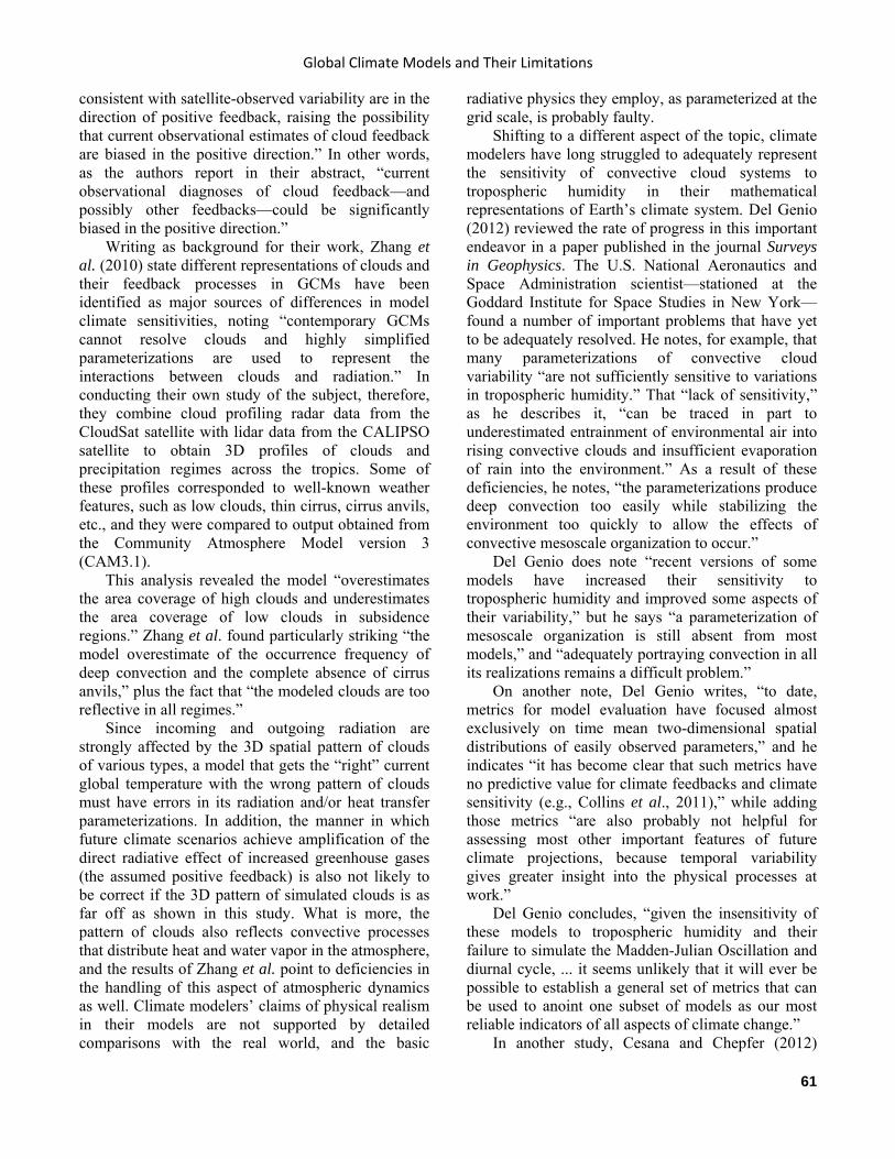
Global Climate Models and Their Limitations
61
consistent with satellite-observed variability are in the direction of positive feedback, raising the possibility that current observational estimates of cloud feedback are biased in the positive direction.” In other words, as the authors report in their abstract, “current observational diagnoses of cloud feedback—and possibly other feedbacks—could be significantly biased in the positive direction.”
Writing as background for their work, Zhang et al. (2010) state different representations of clouds and their feedback processes in GCMs have been identified as major sources of differences in model climate sensitivities, noting “contemporary GCMs cannot resolve clouds and highly simplified parameterizations are used to represent the interactions between clouds and radiation.” In conducting their own study of the subject, therefore, they combine cloud profiling radar data from the CloudSat satellite with lidar data from the CALIPSO satellite to obtain 3D profiles of clouds and precipitation regimes across the tropics. Some of these profiles corresponded to well-known weather features, such as low clouds, thin cirrus, cirrus anvils, etc., and they were compared to output obtained from the Community Atmosphere Model version 3 (CAM3.1).
This analysis revealed the model “overestimates the area coverage of high clouds and underestimates the area coverage of low clouds in subsidence regions.” Zhang et al. found particularly striking “the model overestimate of the occurrence frequency of deep convection and the complete absence of cirrus anvils,” plus the fact that “the modeled clouds are too reflective in all regimes.”
Since incoming and outgoing radiation are strongly affected by the 3D spatial pattern of clouds of various types, a model that gets the “right” current global temperature with the wrong pattern of clouds must have errors in its radiation and/or heat transfer parameterizations. In addition, the manner in which future climate scenarios achieve amplification of the direct radiative effect of increased greenhouse gases (the assumed positive feedback) is also not likely to be correct if the 3D pattern of simulated clouds is as far off as shown in this study. What is more, the pattern of clouds also reflects convective processes that distribute heat and water vapor in the atmosphere, and the results of Zhang et al. point to deficiencies in the handling of this aspect of atmospheric dynamics as well. Climate modelers’ claims of physical realism in their models are not supported by detailed comparisons with the real world, and the basic
radiative physics they employ, as parameterized at the grid scale, is probably faulty.
Shifting to a different aspect of the topic, climate modelers have long struggled to adequately represent the sensitivity of convective cloud systems to tropospheric humidity in their mathematical representations of Earth’s climate system. Del Genio (2012) reviewed the rate of progress in this important endeavor in a paper published in the journal Surveys in Geophysics. The U.S. National Aeronautics and Space Administration scientist—stationed at the Goddard Institute for Space Studies in New York—found a number of important problems that have yet to be adequately resolved. He notes, for example, that many parameterizations of convective cloud variability “are not sufficiently sensitive to variations in tropospheric humidity.” That “lack of sensitivity,” as he describes it, “can be traced in part to underestimated entrainment of environmental air into rising convective clouds and insufficient evaporation of rain into the environment.” As a result of these deficiencies, he notes, “the parameterizations produce deep convection too easily while stabilizing the environment too quickly to allow the effects of convective mesoscale organization to occur.”
Del Genio does note “recent versions of some models have increased their sensitivity to tropospheric humidity and improved some aspects of their variability,” but he says “a parameterization of mesoscale organization is still absent from most models,” and “adequately portraying convection in all its realizations remains a difficult problem.”
On another note, Del Genio writes, “to date, metrics for model evaluation have focused almost exclusively on time mean two-dimensional spatial distributions of easily observed parameters,” and he indicates “it has become clear that such metrics have no predictive value for climate feedbacks and climate sensitivity (e.g., Collins et al., 2011),” while adding those metrics “are also probably not helpful for assessing most other important features of future climate projections, because temporal variability gives greater insight into the physical processes at work.”
Del Genio concludes, “given the insensitivity of these models to tropospheric humidity and their failure to simulate the Madden-Julian Oscillation and diurnal cycle, ... it seems unlikely that it will ever be possible to establish a general set of metrics that can be used to anoint one subset of models as our most reliable indicators of all aspects of climate change.”
In another study, Cesana and Chepfer (2012)

Climate Change Reconsidered II
62
compare the most recent cloud representations of five of the climate models involved in the Coupled Model Intercomparison Project Phase 5 (CMIP5) effort described by Taylor et al. (2012) with real-world satellite-derived observations obtained from the GCM-Oriented CALIPSO Cloud Product (GOCCP), described by Chepfer et al. (2010). According to Cesana and Chepfer, the results indicated: (1) “low- and mid-level altitude clouds are underestimated by all the models (except in the Arctic),” (2) “high altitude cloud cover is overestimated by some models,” (3) “some models shift the altitude of the clouds along the ITCZ by 2 km (higher or lower) compared to observations,” (4) “the models hardly reproduce the cloud free subsidence branch of the Hadley cells,” (5) “the high-level cloud cover is often too large,” (6) “in the tropics, the low-level cloud cover (29% in CALIPSO-GOCCP) is underestimated by all models in subsidence regions (16% to 25%),” and (7) “the pronounced seasonal cycle observed in low-level Arctic clouds is hardly simulated by some models.”
Also writing in 2012, Li et al. (2012) state “representing clouds and cloud climate feedback in global climate models (GCMs) remains a pressing challenge,” but one that must be overcome in order “to reduce and quantify uncertainties associated with climate change projections.” Two of the primary parameters that must be accurately modeled in this regard are cloud ice water content (CIWC) and cloud ice water path (CIWP).
Li et al. performed, in their words, “an observationally based evaluation of the cloud ice water content and path of present-day GCMs, notably 20th century CMIP5 simulations,” after which they compared the results to two recent reanalyses. They used “three different CloudSat + CALIPSO ice water products and two methods to remove the contribution from the convective core ice mass and/or precipitating cloud hydrometeors with variable sizes and falling speeds so that a robust observational estimate can be obtained for model evaluations.”
The 11 U.S. scientists report, “for annual mean CIWP, there are factors of 2–10 in the differences between observations and models for a majority of the GCMs and for a number of regions,” and “systematic biases in CIWC vertical structure occur below the mid-troposphere where the models overestimate CIWC.” They ultimately conclude “neither the CMIP5 ensemble mean nor any individual model performs particularly well,” adding, “there are still a number of models that exhibit very
large biases,” “despite the availability of relevant observations.” Even in cases where “the models may be providing roughly the correct radiative energy budget,” they state “many are accomplishing it by means of unrealistic cloud characteristics of cloud ice mass at a minimum, which in turn likely indicates unrealistic cloud particle sizes and cloud cover.” Li et al. conclude “cloud feedback will undoubtedly still represent a key uncertainty in [even] the next IPCC assessment report.”
Cesana et al. (2012) state “low-level clouds frequently occur in the Arctic and exert a large influence on Arctic surface radiative fluxes and Arctic climate feedbacks,” noting that during winter, in particular, surface net longwave radiation (FLW,NET) has a bimodal distribution, with extremes that have been termed “radiatively clear” and “radiatively opaque.” They note Arctic ice clouds “tend to have small optical depths and a weak influence on FLW,NET,” which explains the “radiatively clear” condition, whereas Arctic liquid-containing clouds “generally have large optical depths and a dominant influence on FLW,NET (Shupe and Intrieri, 2004),” which explains the “radiatively opaque” condition, as discussed by Doyle et al. (2011).
Against this backdrop, Cesana et al. employed real-world Cloud-Aerosol Lidar and Infrared Pathfinder Satellite Observation (CALIPSO) data to document cloud phases over the Arctic basin (60–82°N) during the five-year period 2006–2011, after which they used the results they obtained “to evaluate the influence of Arctic cloud phase on Arctic cloud radiative flux biases in climate models.” The five researchers report their evaluation of climate models participating in the most recent Coupled Model Inter-comparison Project (Taylor et al., 2012) revealed “most climate models are not accurately representing the bimodality of FLW,NET in non-summer seasons.” Even when advanced microphysical schemes that predict cloud phase have been used, such as those currently employed in the fifth version of the Community Atmosphere Model (CAM5, Neale et al., 2010), “insufficient liquid water was predicted.”
Cesana et al. conclude “the simple prescribed relationships between cloud phase and temperature that have historically been used in climate models are incapable of reproducing the Arctic cloud phase observations described here,” which must inevitably lead to similarly inaccurate values of “Arctic surface radiative fluxes and Arctic climate feedbacks” when employed in current climate models.
Also focusing on low-level clouds were Nam et

Global Climate Models and Their Limitations
63
al. (2012), who write the response of low-level clouds has long been identified as “a key source of uncertainty for model cloud feedbacks under climate change,” citing the work of Bony and Dufresne (2005), Webb et al. (2006), Wyant et al. (2006), and Medeiros et al. (2008). They state “the ability of climate models to simulate low-clouds and their radiative properties” plays a large role in assessing “our confidence in climate projections.” Nam et al. analyzed “outputs from multiple climate models participating in the Fifth phase of the Coupled Model Intercomparison Project (CMIP5) using the Cloud Feedback Model Intercomparison Project Observations Simulator Package (COSP), and compared them with different satellite data sets,” including “CALIPSO lidar observations, PARASOL mono-directional reflectances, and CERES radiative fluxes at the top of the atmosphere.”
The comparison revealed “the current generation of climate models still experiences difficulties in predicting the low-cloud cover and its radiative effects.” In particular, they report the models: (1) “under-estimate low-cloud cover in the tropics,” (2) “over-estimate optical thickness of low-clouds, particularly in shallow cumulus regimes,” (3) “poorly represent the dependence of the low-cloud vertical structure on large-scale environmental conditions,” and (4) “predict stratocumulus-type of clouds in regimes where shallow cumulus cloud-types should prevail.” However, they say “the impact of these biases on the Earth’s radiation budget ... is reduced by compensating errors,” including “the tendency of models to under-estimate the low-cloud cover and to over-estimate the occurrence of mid- and high-clouds above low-clouds.”
Convective-type clouds and precipitation, especially when occurring over land areas, in the tropics, or during the warm season, have a strong diurnal cycle in phase with solar heating. People living in coastal regions are familiar with the diurnal cycle via the sea-breeze phenomenon. Unfortunately, models have difficulty representing the diurnal component of convection. Stratton and Stirling (2012) devised a better way to represent this phenomenon in an atmospheric general circulation model. In particular, they improved the rate at which environmental air and cloud air mix (entrainment). They also revised the mass flux over land in order to improve the timing and strength of convection influenced by diurnal heating.
In order to test the impact of the changes made to the diurnal convection scheme on the precipitation
climatology of a model, Stratton and Stirling used a GCM with a horizontal resolution of less than two degrees in latitude and longitude and ran two ten-year simulations. The first was a control run with the model as it was provided to them. Then a ten-year run was performed with the new convective parameterizations added. Results were compared with observed precipitation, as derived from output provided by the Tropical Rainfall Measurement Mission (TRMM) satellite.
According to the authors, the control run (Figure 1.3.4.1) “tends to lack precipitation over India and have too much precipitation over tropical land in Africa and in South America. The new run has generally reduced the precipitation over tropical land, tending to improve agreement with CMAP” (CMAP is an acronym for the observations). In the mid-latitudes though, there were regions (e.g., western Russia) where the new parameterization improved the model results, but other places where the new parameterization was worse (e.g., Europe). The results also did not noticeably alter the general circulation.
Stratton and Stirling improved the attendant physics associated with convection and in general improved the climatological representation of precipitation. But there were still differences in comparison with observed precipitation. In some regions, the new convective scheme performance was not as good. Improvement was not uniform, even though the model was overall closer to reality.
The new parameterizations may have done a good job of representing precipitation over short time-scales, but over longer time-scales it still did not represent the climatology of precipitation very well.
Ahlgrimm and Forbes (2012) investigated an irradiance bias in the European Centre for Medium Range Forecasting (ECMWF) GCM, focusing on the Southern Great Plains of the USA. This GCM was built to generate daily weather predictions. In one experiment, the authors compared measured radiation daily in 2004–2009 from the Atmospheric Radiation Measurement Site (ARM) in the Southern Great Plains (SGP) (Figure 1.3.4.2). In the second, they compared the ECMWF model output to observations of clouds, radiation, and the state of the atmosphere archived as the Climate Modelling Best Estimate product from 1997–2009. Ahlgrimm and Forbes selected 146 days when fair weather cumulus clouds dominated the Southern Great Plains. They compared these to the same days run using the ECMWF model initialized the day before and using the 18–42 hour
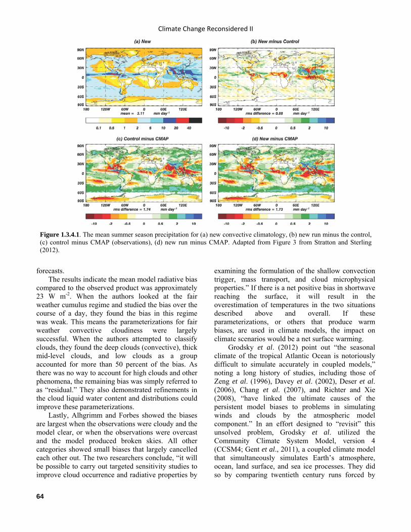
Climate Change Reconsidered II
64
forecasts. The results indicate the mean model radiative bias
compared to the observed product was approximately 23 W m-2. When the authors looked at the fair weather cumulus regime and studied the bias over the course of a day, they found the bias in this regime was weak. This means the parameterizations for fair weather convective cloudiness were largely successful. When the authors attempted to classify clouds, they found the deep clouds (convective), thick mid-level clouds, and low clouds as a group accounted for more than 50 percent of the bias. As there was no way to account for high clouds and other phenomena, the remaining bias was simply referred to as “residual.” They also demonstrated refinements in the cloud liquid water content and distributions could improve these parameterizations.
Lastly, Alhgrimm and Forbes showed the biases are largest when the observations were cloudy and the model clear, or when the observations were overcast and the model produced broken skies. All other categories showed small biases that largely cancelled each other out. The two researchers conclude, “it will be possible to carry out targeted sensitivity studies to improve cloud occurrence and radiative properties by
examining the formulation of the shallow convection trigger, mass transport, and cloud microphysical properties.” If there is a net positive bias in shortwave reaching the surface, it will result in the overestimation of temperatures in the two situations described above and overall. If these parameterizations, or others that produce warm biases, are used in climate models, the impact on climate scenarios would be a net surface warming.
Grodsky et al. (2012) point out “the seasonal climate of the tropical Atlantic Ocean is notoriously difficult to simulate accurately in coupled models,” noting a long history of studies, including those of Zeng et al. (1996), Davey et al. (2002), Deser et al. (2006), Chang et al. (2007), and Richter and Xie (2008), “have linked the ultimate causes of the persistent model biases to problems in simulating winds and clouds by the atmospheric model component.” In an effort designed to “revisit” this unsolved problem, Grodsky et al. utilized the Community Climate System Model, version 4 (CCSM4; Gent et al., 2011), a coupled climate model that simultaneously simulates Earth’s atmosphere, ocean, land surface, and sea ice processes. They did so by comparing twentieth century runs forced by
Figure 1.3.4.1. The mean summer season precipitation for (a) new convective climatology, (b) new run minus the control, (c) control minus CMAP (observations), (d) new run minus CMAP. Adapted from Figure 3 from Stratton and Sterling (2012).
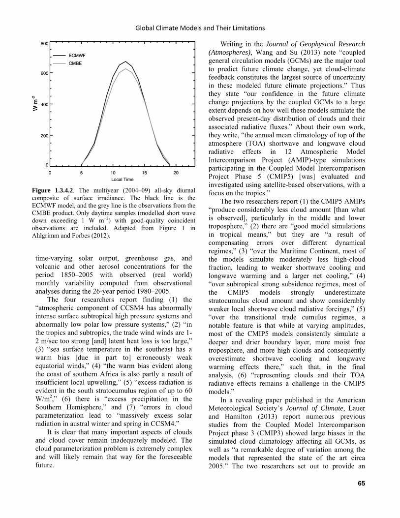
Global Climate Models and Their Limitations
65
time-varying solar output, greenhouse gas, and volcanic and other aerosol concentrations for the period 1850–2005 with observed (real world) monthly variability computed from observational analyses during the 26-year period 1980–2005.
The four researchers report finding (1) the “atmospheric component of CCSM4 has abnormally intense surface subtropical high pressure systems and abnormally low polar low pressure systems,” (2) “in the tropics and subtropics, the trade wind winds are 1-2 m/sec too strong [and] latent heat loss is too large,” (3) “sea surface temperature in the southeast has a warm bias [due in part to] erroneously weak equatorial winds,” (4) “the warm bias evident along the coast of southern Africa is also partly a result of insufficient local upwelling,” (5) “excess radiation is evident in the south stratocumulus region of up to 60 W/m2,” (6) there is “excess precipitation in the Southern Hemisphere,” and (7) “errors in cloud parameterization lead to “massively excess solar radiation in austral winter and spring in CCSM4.”
It is clear that many important aspects of clouds and cloud cover remain inadequately modeled. The cloud parameterization problem is extremely complex and will likely remain that way for the foreseeable future.
Writing in the Journal of Geophysical Research (Atmospheres), Wang and Su (2013) note “coupled general circulation models (GCMs) are the major tool to predict future climate change, yet cloud-climate feedback constitutes the largest source of uncertainty in these modeled future climate projections.” Thus they state “our confidence in the future climate change projections by the coupled GCMs to a large extent depends on how well these models simulate the observed present-day distribution of clouds and their associated radiative fluxes.” About their own work, they write, “the annual mean climatology of top of the atmosphere (TOA) shortwave and longwave cloud radiative effects in 12 Atmospheric Model Intercomparison Project (AMIP)-type simulations participating in the Coupled Model Intercomparison Project Phase 5 (CMIP5) [was] evaluated and investigated using satellite-based observations, with a focus on the tropics.”
The two researchers report (1) the CMIP5 AMIPs “produce considerably less cloud amount [than what is observed], particularly in the middle and lower troposphere,” (2) there are “good model simulations in tropical means,” but they are “a result of compensating errors over different dynamical regimes,” (3) “over the Maritime Continent, most of the models simulate moderately less high-cloud fraction, leading to weaker shortwave cooling and longwave warming and a larger net cooling,” (4) “over subtropical strong subsidence regimes, most of the CMIP5 models strongly underestimate stratocumulus cloud amount and show considerably weaker local shortwave cloud radiative forcings,” (5) “over the transitional trade cumulus regimes, a notable feature is that while at varying amplitudes, most of the CMIP5 models consistently simulate a deeper and drier boundary layer, more moist free troposphere, and more high clouds and consequently overestimate shortwave cooling and longwave warming effects there,” such that, in the final analysis, (6) “representing clouds and their TOA radiative effects remains a challenge in the CMIP5 models.”
In a revealing paper published in the American Meteorological Society’s Journal of Climate, Lauer and Hamilton (2013) report numerous previous studies from the Coupled Model Intercomparison Project phase 3 (CMIP3) showed large biases in the simulated cloud climatology affecting all GCMs, as well as “a remarkable degree of variation among the models that represented the state of the art circa 2005.” The two researchers set out to provide an
Figure 1.3.4.2. The multiyear (2004–09) all-sky diurnal composite of surface irradiance. The black line is the ECMWF model, and the grey line is the observations from the CMBE product. Only daytime samples (modelled short wave down exceeding 1 W m−2) with good-quality coincident observations are included. Adapted from Figure 1 in Ahlgrimm and Forbes (2012).

Climate Change Reconsidered II
66
update by describing the progress that has been made in recent years by comparing mean cloud properties, interannual variability, and the climatological seasonal cycle from the CMIP5 models with results from comparable CMIP3 experiments, as well as with actual satellite observations.
Lauer and Hamilton conclude “the simulated cloud climate feedbacks activated in global warming projections differ enormously among state-of-the-art models,” while noting “this large degree of disagreement has been a constant feature documented for successive generations of GCMs from the time of the first Intergovernmental Panel on Climate Change assessment through the CMIP3 generation models used in the fourth IPCC assessment.” They add, “even the model-simulated cloud climatologies for present-day conditions are known to depart significantly from observations and, once again, the variation among models is quite remarkable (e.g., Weare, 2004; Zhang et al., 2005; Waliser et al., 2007, 2009; Lauer et al., 2010; Chen et al., 2011).”
The two researchers determined (1) “long-term mean vertically integrated cloud fields have quite significant deficiencies in all the CMIP5 model simulations,” (2) “both the CMIP5 and CMIP3 models display a clear bias in simulating too high LWP [liquid water path] in mid-latitudes,” (3) “this bias is not reduced in the CMIP5 models,” (4) there have been “little to no changes in the skill of reproducing the observed LWP and CA [cloud amount],” (5) “inter-model differences are still large in the CMIP5 simulations,” and (6) “there is very little to no improvement apparent in the tropical and subtropical regions in CMIP5.”
Lauer and Hamilton indicate there is “only very modest improvement in the simulated cloud climatology in CMIP5 compared with CMIP3,” adding even this slightest of improvements “is mainly a result of careful model tuning rather than an accurate fundamental representation of cloud processes in the models.”
It would therefore appear, given the findings described in this section, that the outlook for adequately modeling clouds and cloud processes must still be characterized as cloudy. References Ahlgrimm, M. and Forbes, R. 2012. The Impact of Low Clouds on Surface Shortwave Radiation in the ECMWF Model. Monthly Weather Review 140: 3783–3794.
Ayers, G.P. and Gillett, R.W. 2000. DMS and its oxidation products in the remote marine atmosphere: implications for climate and atmospheric chemistry. Journal of Sea Research 43: 275–286.
Bony, S. and Dufresne, J. 2005. Marine boundary layer clouds at the heart of tropical cloud feedback uncertainties in climate models. Geophysical Research Letters 32: 10.1029/2005GL023851.
Cesana, G. and Chepfer, H. 2012. How well do climate models simulate cloud vertical structure? A comparison between CALIPSO-GOCCP satellite observations and CMIP5 models. Geophysical Research Letters 39: 10.1029/2012GL053153.
Cesana, G., Kay, J.E., Chepfer, H., English, J.M., and de Boer, G. 2012. Ubiquitous low-level liquid-containing Arctic clouds: New observations and climate model constraints from CALIPSO-GOCCP. Geophysical Research Letters 39: 10.1029/2012GL053385.
Cess, R.D. et al. 1990. Intercomparison and interpretation of climate feedback processes in 19 atmospheric general circulation models. Journal of Geophysical Research 95: 16601–16615.
Chang, C.-Y., Carton, J.A., Grodsky, S.A., and Nigam, S. 2007. Seasonal climate of the tropical Atlantic sector in the NCAR Community Climate System Model 3: Error structure and probable causes of errors. Journal of Climate 20: 1053–1070.
Charlson, R.J., Lovelock, J.E., Andrea, M.O., and Warren, S.G. 1987. Oceanic phytoplankton, atmospheric sulfur, cloud albedo and climate. Nature 326: 655–661.
Chen, W.-T., Woods, C.P., Li, J.-L.F., Waliser, D.E., Chern, J.-D., Tao, W.-K., Jiang, J.H., and Tompkins, A.M. 2011. Partitioning CloudSat ice water content for comparison with upper tropospheric ice in global atmospheric models. Journal of Geophysical Research 116: 10.1029/2010JD015179.
Chou, M.-D., Lindzen, R.S., and Hou, A.Y. 2002. Reply to: “Tropical cirrus and water vapor: an effective Earth infrared iris feedback?” Atmospheric Chemistry and Physics 2: 99–101.
Collins, M., Booth, B.B.B., Bhaskaran, B., Harris, G.R., Murphy, J.M., Sexton, D.M.H., and Webb, M.J. 2011. Climate model errors, feedbacks and forcings: a comparison of perturbed physics and multi-model ensembles. Climate Dynamics 36: 1737–1766.
Davey, M.K., Huddleston, M., Sperber, K. R., Braconnot, P., Bryan, F., Chen, D., Colman, R., Cooper, C., Cubasch, U., Delecluse, P., DeWitt, D., Fairhead, L., Flato, G., Gordon, C., Hogan, T., Ji, M., Kimoto, M., Kitoh, A., Knutson, T. R., Latif, M., Le Treut, H., Li, T., Manabe, S.,
Global Climate Models and Their Limitations
67
Mechoso, C. R., Meehl, G. A., Power, S. B., Roeckner, E., Terray, L., Vintzileos, A., Voss, R., Wang, B., Washington, W. M., Yoshikawa, I., Yu, J. Y., Yukimoto, S., and Zebiak, S. E. 2002. STOIC: A study of coupled model climatology and variability in tropical ocean regions. Climate Dynamics 18: 403–420.
Del Genio, A.D. 2012. Representing the sensitivity of convective cloud systems to tropospheric humidity in general circulation models. Surveys in Geophysics 33: 637–656.
Deser, C., Capotondi, A., Saravanan, R., and Phillips, A. 2006. Tropical Pacific and Atlantic climate variability in CCSM3. Journal of Climate 19: 403–420.
Doyle, J.G., Lesins, G., Thakray, C.P., Perro, C., Nott, G.J., Duck, T.J., Damoah, R., and Drummond, J.R. 2011. Water vapor intrusions into the High Arctic during winter. Geophysical Research Letters 38: 10.1029/2011GL047493.
Dufresne, J.-L. and Bony, S. 2008. An assessment of the primary sources of spread of global warming estimates from coupled atmosphere-ocean models. Journal of Climate 21: 5135–5144.
Forster, P.M., and Taylor, K.E. 2006. Climate forcings and climate sensitivities diagnosed from coupled climate model integrations, Journal of Climate 19: 6181–6194.
Fu, Q., Baker, M. and Hartmann, D.L. 2002. Tropical cirrus and water vapor: an effective Earth infrared iris feedback? Atmospheric Chemistry and Physics 2: 31–37.
Gent, P.R., Danabasoglu, G., Donner, L.M., Holland, M.M., Hunke, E.C., Jayne, S.R., Lawrence, D.M., Neale, R.B., Rasch, P.J., Vertenstein, M., Worley, P.H., Yang, Z.-L., and Zhang M. 2011. The Community Climate System Model version 4. Journal of Climate 24: 4973–4991.
Gordon, C.T., Rosati, A., and Gudgel, R. 2000. Tropical sensitivity of a coupled model to specified ISCCP low clouds. Journal of Climate 13: 2239–2260.
Grabowski, W.W. 2000. Cloud microphysics and the tropical climate: Cloud-resolving model perspective. Journal of Climate 13: 2306–2322.
Grassl, H. 2000. Status and improvements of coupled general circulation models. Science 288: 1991–1997.
Grodsky, S.A., Carton, J.A., Nigam, S., and Okumura, Y.M. 2012. Tropical Atlantic biases in CCSM4. Journal of Climate 25: 3684–3701.
Groisman, P.Ya., Bradley, R.S., and Sun, B. 2000. The relationship of cloud cover to near-surface temperature and humidity: Comparison of GCM simulations with empirical data. Journal of Climate 13: 1858–1878.
Harries, J.E. 2000. Physics of the Earth’s radiative energy
balance. Contemporary Physics 41: 309–322.
Hartmann, D.L. and Michelsen, M.L. 2002. No evidence for IRIS. Bulletin of the American Meteorological Society 83: 249–254.
Idso, S.B. 1990. A role for soil microbes in moderating the carbon dioxide greenhouse effect? Soil Science 149: 179–180.
Lane, D.E., Somerville, R.C.J., and Iacobellis, S.F. 2000. Sensitivity of cloud and radiation parameterizations to changes in vertical resolution. Journal of Climate 13: 915–922.
Lauer, A. and Hamilton, K. 2013. Simulating clouds with global climate models: A comparison of CMIP5 results with CMIP3 and satellite data. Journal of Climate 26: 3823–3845.
Lauer, A., Hamilton, K., Wang, Y., Phillips, V.T.J., and Bennartz, R. 2010. The impact of global warming on marine boundary layer clouds over the eastern Pacific—A regional model study. Journal of Climate 23: 5844–5863.
L’Ecuyer, T.S. and Stephens, G.L. 2007. The tropical atmospheric energy budget from the TRMM perspective. Part II: Evaluating GCM representations of the sensitivity of regional energy and water cycles to the 1998-99 ENSO cycle. Journal of Climate 20: 4548–4571.
Li, J.-L.F., Waliser, D.E., Chen, W.-T., Guan, B., Kubar, T., Stephens, G., Ma, H.-Y., Deng, M., Donner, L., Seman, C., and Horowitz, L. 2012. An observationally based evaluation of cloud ice water in CMIP3 and CMIP5 GCMs and contemporary reanalyses using contemporary satellite data. Journal of Geophysical Research 117: 10.1029/2012JD017640.
Lindzen, R.S., Chou, M.-D., and Hou, A.Y. 2001. Does the earth have an adaptive infrared iris? Bulletin of the American Meteorological Society 82: 417–432.
Medeiros, B., Stevens, B., Held, I., Zhao, M., Williamson, D., Olson, J., and Bretherton, C. 2008. Aquaplanets, climate sensitivity, and low clouds. Journal of Climate 21: 4974–4991.
Nam, C., Bony, S., Dufresne, J.-L., and Chepfer, H. 2012. The ‘too few, too bright’ tropical low-cloud problem in CMIP5 models. Geophysical Research Letters 39: 10.1029/2012GL053421.
Neale, R.B., et al. 2010. Description of the NCAR Community Atmosphere Model (CAM 5.0). Technical Note 486+STR. National Center for Atmospheric Research, Boulder, Colorado, USA.
O’Dowd, C.D., Facchini, M.C., Cavalli, F., Ceburnis, D., Mircea, M., Decesari, S., Fuzzi, S., Yoon, Y.J., and Putaud, J.-P. 2004. Biogenically driven organic contribution to

Climate Change Reconsidered II
68
marine aerosol. Nature 431: 676–680.
Randall, D., Khairoutdinov, M., Arakawa, A., and Grabowski, W. 2003. Breaking the cloud parameterization deadlock. Bulletin of the American Meteorological Society 84: 1547–1564.
Randall, D.A., Wood, R.A., Bony, S., Coleman, R., Fichefet, T., Fyfe, J., Kattsov, V., Pitman, A., Shukla, J., Srinivasan, J., Stouffer, R.J., Sumi, A., and Taylor, K.E. 2007. Chapter 8: Climate Models and Their Evaluation. In: Climate Change 2007: The Physical Science Basis. Contribution of Working Group I to the Fourth Assessment Report of the Intergovernmental Panel on Climate Change. Cambridge University Press, Cambridge, United Kingdom.
Richter, I. and Xie, S.-P. 2008. On the origin of equatorial Atlantic biases in coupled general circulation models. Climate Dynamics 31: 587–598.
Riehl, H. and Malkus, J. 1958. On the heat balance in the equatorial trough zone. Geophysica 6: 503–538.
Senior, C.A. and Mitchell, J.F.B. 1993. CO2 and climate: The impact of cloud parameterization. Journal of Climate 6: 393–418.
Shupe, M.D. and Intrieri, J.M. 2004. Cloud radiative forcing of the Arctic surface: The influence of cloud properties, surface albedo, and solar zenith angle. Journal of Climate 17: 616–628.
Siebesma, A.P., Jakob, C., Lenderink, G., Neggers, R.A.J., Teixeira, J., van Meijgaard, E., Calvo, J., Chlond, A., Grenier, H., Jones, C., Kohler, M., Kitagawa, H., Marquet, P., Lock, A.P., Muller, F., Olmeda, D., and Severijns, C. 2004. Cloud representation in general-circulation models over the northern Pacific Ocean: A EUROCS intercomparison study. Quarterly Journal of the Royal Meteorological Society 130: 3245–3267.
Soden, B.J. and Held, I.M. 2006. An assessment of climate feedbacks in coupled ocean-atmosphere models. Journal of Climate 19: 3354–3360.
Spencer, R.W. and Braswell, W.D. 2008.Potential biases in feedback diagnosis from observational data: A simple model demonstration. Journal of Climate 21: 5624–5628.
Spencer, R.W., Braswell, W.D., Christy, J.R., and Hnilo, J. 2007. Cloud and radiation budget changes associated with tropical intraseasonal oscillations. Geophysical Research Letters 34: L15707, doi:10.1029/2007GLO296998.
Stephens, G.L. 2005. Clouds feedbacks in the climate system: A critical review. Journal of Climate 18: 237–273.
Stratton, R.A. and Stirling, A.J. 2012. Improving the diurnal cycle of convection in GCMs. Quarterly Journal of the Royal Meteorological Society 138: 1121–1134.
Taylor, K.E., Stouffer, R.J., and Meehl, G.A. 2012. An overview of CMIP5 and the experimental design. Bulletin of the American Meteorological Society 93: 485–498.
Waliser, D.E., Seo, K.-W., Schubert, S., and Njoku, E. 2007. Global water cycle agreement in the climate models assessed in the IPCC AR4. Geophysical Research Letters 34: 10.1029/2007GL030675.
Waliser, D.E., Li, J.-L.F., Woods, C.P., Austin, R.T., Bacmeister, J., Chern, J., Del Genio, A., Jiang, J.H., Kuang, Z., Meng, H., Minnis, P., Platnick, S., Rossow, W.B., Stephens, G.L., Sun-Mack, S., Tao, W.-K., Tompkins, A.M., Vane, D.G., Walker, C., and Wu, D. 2009. Cloud ice: A climate model challenge with signs and expectations of progress. Journal of Geophysical Research 114: 10.1029/2008JD010015.
Wang, H. and Su, W. 2013. Evaluating and understanding top of the atmosphere cloud radiative effects in Intergovernmental Panel on Climate Change (IPCC) Fifth Assessment Report (AR5) Coupled Model Intercomparison Project Phase 5 (CMIP5) models using satellite observations. Journal of Geophysical Research: Atmospheres 118: 683–699.
Weare, B.C. 2004. A comparison of AMIP II model cloud layer properties with ISCCP D2 estimates. Climate Dynamics 22: 281–292.
Webb, M.J., Senior, C.A., Sexton, D.M.H., Ingram, W.J., Williams, K.D., Ringer, M.A., McAvaney, B.J., Colman, R., Soden, B.J., Gudgel, R., Knutson, T., Emori, S., Ogura, T., Tsushima, Y., Andronova, N., Li, B., Musat, I., Bony, S., and Taylor, K.E. 2006. On the contribution of local feedback mechanisms to the range of climate sensitivity in two GCM ensembles. Climate Dynamics 27: 17–38.
Webster, P.J. and Stephens, G.L. 1984. Cloud-radiation feedback and the climate problem. In Houghton, J. (Ed.) The Global Climate. Cambridge University Press. 63–78.
Wyant, M., Khairoutdinov, M., and Bretherton, C. 2006. Climate sensitivity and cloud response of a GCM with a superparameterization. Geophysical Research Letters 33: 10.1029/2005GL025464.
Zeng, N., Dickinson, R.E., and Zeng, X. 1996. Climate impact of Amazon deforestation—A mechanistic model study. Journal of Climate 9: 859–883.
Zhang, M.H., Lin, W.Y., Klein, S.A., Bacmeister, J.T., Bony, S., Cederwall, R.T., Del Genio, A.D., Hack, J.J., Loeb, N.G., Lohmann, U., Minnis, P., Musat, I., Pincus, R., Stier, P., Suarez, M.J., Webb, M.J., Wu, J.B., Xie, S.C., Yao, M.-S., and Yang, J.H. 2005. Comparing clouds and their seasonal variations in 10 atmospheric general circulation models with satellite measurements. Journal of Geophysical Research 110: D15S02, doi:10.1029/2004 JD005021.

Global Climate Models and Their Limitations
69
Zhang, Y., Klein, S.A., Boyle, J., and Mace, G.G. 2010. Evaluation of tropical cloud and precipitation statistics of Community Atmosphere Model version 3 using CloudSat and CALIPSO data. Journal of Geophysical Research 115: doi:10.1029/2009JD012006.
Zhou, Y.P., Tao, W.-K., Hou, A.Y., Olson, W.S., Shie, C.-L., Lau, K.-M., Chou, M.-D., Lin, X., and Grecu, M. 2007. Use of high-resolution satellite observations to evaluate cloud and precipitation statistics from cloud-resolving model simulations. Part I: South China Sea monsoon experiment. Journal of the Atmospheric Sciences 64: 4309–4329.
1.3.5 Precipitation 1.3.5.1 Precipitation Correctly simulating future precipitation has proven to be an extremely difficult task for modelers. One reason for the lack of success in this area is inadequate model resolution on both vertical and horizontal spatial scales, a limitation that forces climate modelers to parameterize the large-scale effects of processes (such as deep convection, which is the source of most precipitation) that occur on smaller scales than the models are capable of simulating. But there are other problems as well that result in vast differences between model projections and real-world observations. This section documents such problems and variances as they relate to model projections of precipitation.
In an early study of the subject, Lebel et al. (2000) compared rainfall simulations produced by a GCM with real-world observations from West Africa for the period 1960–1990. Their analysis revealed the model output was affected by a number of temporal and spatial biases that led to significant differences between observed and modeled data. The simulated rainfall totals, for example, were significantly greater than what was typically observed, exceeding real-world values by 25 percent during the dry season and 75 percent during the rainy season. In addition, the seasonal cycle of precipitation was not well simulated, as the researchers found the simulated rainy season began too early and the increase in precipitation was not rapid enough. Shortcomings were also evident in the GCM’s inability to accurately simulate convective rainfall events, as it typically predicted too much precipitation. Furthermore, it was found “inter-annual variability [was] seriously disturbed in the GCM as compared to what it [was] in the observations.” As for why the GCM performed so
poorly in these several respects, Lebel et al. gave two main reasons: parameterization of rainfall processes in the GCM was much too simple, and spatial resolution was much too coarse.
Lau et al. (2006) considered the Sahel drought of the 1970s–1990s to provide “an ideal test bed for evaluating the capability of CGCMs [coupled general circulation models] in simulating long-term drought, and the veracity of the models’ representation of coupled atmosphere-ocean-land processes and their interactions.” They chose to “explore the roles of sea surface temperature coupling and land surface processes in producing the Sahel drought in CGCMs that participated in the twentieth-century coupled climate simulations of the Intergovernmental Panel on Climate Change [IPCC] Assessment Report 4,” in which the 19 CGCMs “are driven by combinations of realistic prescribed external forcing, including anthropogenic increase in greenhouse gases and sulfate aerosols, long-term variation in solar radiation, and volcanic eruptions.”
The climate scientists found “only eight models produce a reasonable Sahel drought signal, seven models produce excessive rainfall over [the] Sahel during the observed drought period, and four models show no significant deviation from normal.” In addition, they report, “even the model with the highest skill for the Sahel drought could only simulate the increasing trend of severe drought events but not the magnitude, nor the beginning time and duration of the events.” All 19 of the CGCMs employed in the IPCC’s Fourth Assessment Report, in other words, failed to adequately simulate the basic characteristics of “one of the most pronounced signals of climate change” of the past century—as defined by its start date, severity and duration.”
Writing in Science, Wentz et al. (2007) noted the Coupled Model Intercomparison Project, as well as various climate modeling analyses, predicted an increase in precipitation on the order of 1 to 3 percent per °C of surface global warming. They decided to see what had happened in the real world in this regard over the prior 19 years (1987–2006) of supposedly unprecedented global warming, when data from the Global Historical Climatology Network and satellite measurements of the lower troposphere indicated there had been a global temperature rise on the order of 0.20°C per decade.
Using satellite observations obtained from the Special Sensor Microwave Imager (SSM/I), the four Remote Sensing Systems scientists derived precipitation trends for the world’s oceans over this

Climate Change Reconsidered II
70
period. Using data obtained from the Global Precipitation Climatology Project acquired from both satellite and rain gauge measurements, they derived precipitation trends for Earth’s continents. Combining the results of these two endeavors, they derived a real-world increase in precipitation on the order of 7 percent per °C of surface global warming, somewhere between 2.3 and 7.0 times larger than what is predicted by state-of-the-art climate models.
How was this discrepancy to be resolved? Wentz et al. conclude the only way to bring the two results into harmony was for there to have been a 19-year decline in global wind speeds. But when looking at the past 19 years of SSM/I wind retrievals, they found just the opposite, an increase in global wind speeds. In quantitative terms, the two results were about as opposite as they could possibly be: “when averaged over the tropics from 30°S to 30°N, the winds increased by 0.04 m s-1 (0.6 percent) decade-1, and over all oceans the increase was 0.08 m s-1 (1.0 percent) decade-1,” while global coupled ocean-atmosphere models or GCMs, in their words, “predict that the 1987-to-2006 warming should have been accompanied by a decrease in winds on the order of 0.8 percent decade-1.”
Wentz et al. state, “the reason for the discrepancy between the observational data and the GCMs is not clear.” They also observe this dramatic difference between the real world of nature and the virtual world of climate modeling “has enormous impact” and the questions raised by the discrepancy “are far from being settled.”
In a separate paper published that year, Allan and Soden (2007) quantified trends in precipitation within ascending and descending branches of the planet’s tropical circulation and compared their results with simulations of the present day and projections of future changes provided by up to 16 state-of-the-art climate models. The precipitation data for this analysis came from the Global Precipitation Climatology Project (GPCP) of Adler et al. (2003) and the Climate Prediction Center Merged Analysis of Precipitation (CMAP) data of Xie and Arkin (1998) for the period 1979–2006, while for the period 1987–2006 the data came from the monthly mean intercalibrated Version 6 Special Sensor Microwave Imager (SSM/I) precipitation data described by Wentz et al. (2007).
The researchers report “an emerging signal of rising precipitation trends in the ascending regions and decreasing trends in the descending regions are detected in the observational datasets,” but “these
trends are substantially larger in magnitude than present-day simulations and projections into the 21st century,” especially in the case of the descending regions. More specifically, for the tropics “the GPCP trend is about 2–3 times larger than the model ensemble mean trend, consistent with previous findings (Wentz et al., 2007) and also supported by the analysis of Yu and Weller (2007),” who additionally contended “observed increases of evaporation over the ocean are substantially greater than those simulated by climate models.” In addition, Allan and Soden note “observed precipitation changes over land also appear larger than model simulations over the 20th century (Zhang et al., 2007).”
Noting the difference between the models and real-world measurements “has important implications for future predictions of climate change,” Allan and Soden state “the discrepancy cannot be explained by changes in the reanalysis fields used to subsample the observations but instead must relate to errors in the satellite data or in the model parameterizations.” This dilemma also was faced by Wentz et al. (2007), and they too state the resolution of the issue “has enormous impact” and likewise conclude the questions raised by the discrepancy “are far from being settled.”
According to Lin (2007), “a good simulation of tropical mean climate by the climate models is a prerequisite for their good simulations/predictions of tropical variabilities and global teleconnections,” but “unfortunately, the tropical mean climate has not been well simulated by the coupled general circulation models (CGCMs) used for climate predictions and projections.” They note “most of the CGCMs produce a double-intertropical convergence zone (ITCZ) pattern” and they acknowledge “a synthetic view of the double-ITCZ problem is still elusive.”
Lin analyzed tropical mean climate simulations of the 20-year period 1979–1999 provided by 22 IPCC Fourth Assessment Report CGCMs, together with concurrent Atmospheric Model Intercomparison Project (AMIP) runs from 12 of them. This revealed, in Lin’s words, that “most of the current state-of-the-art CGCMs have some degree of the double-ITCZ problem, which is characterized by excessive precipitation over much of the Tropics (e.g., Northern Hemisphere ITCZ, Southern Hemisphere SPCZ [South Pacific Convergence Zone], Maritime Continent, and equatorial Indian Ocean), and often associated with insufficient precipitation over the equatorial Pacific,” as well as “overly strong trade winds, excessive LHF [latent heat flux], and

Global Climate Models and Their Limitations
71
insufficient SWF [shortwave flux], leading to significant cold SST (sea surface temperature) bias in much of the tropical oceans.”
Lin further notes “most of the models also simulate insufficient latitudinal asymmetry in precipitation and SST over the eastern Pacific and Atlantic Oceans,” and “the AMIP runs also produce excessive precipitation over much of the Tropics including the equatorial Pacific, which also leads to overly strong trade winds, excessive LHF, and insufficient SWF.” All of this suggests “the excessive tropical precipitation is an intrinsic error of the atmospheric models,” Lin writes, adding, “over the eastern Pacific stratus region, most of the models produce insufficient stratus-SST feedback associated with insufficient sensitivity of stratus cloud amount to SST.”
With the solutions to all of these longstanding problems continuing to remain “elusive,” and with Lin suggesting the sought-for solutions are in fact prerequisites for “good simulations/predictions” of future climate, there is significant reason to conclude that current state-of-the-art CGCM predictions of CO2-induced global warming should not be considered reliable.
Lavers et al. (2009) examined the predictive skill of eight seasonal climate forecast models developed at various European climate centers. Specifically, they assessed the predictability of monthly precipitation “retrospective forecasts” or hindcasts, composed of multiple nine-month projections initialized during each month of the year over the period 1981–2001. They compared the projections against real-world precipitation values obtained from Global Precipitation Climatology Center data. In addition, they conducted a virtual-world analysis, where the output of one of the models was arbitrarily assumed to be the truth and the average of the rest of the models was assumed to be the predictor.
These analyses indicate that in the virtual world of the climate models, there was quite good skill over the first two weeks of the forecast, when the spread of ensemble model members was small, but there was a large drop off in predictive skill in the second 15-day period. Things were even worse in the real world, where the models had negligible skill over land at a 31-day lead time, which the researchers describe as being “a relatively short lead time in terms of seasonal climate prediction.” The three researchers conclude that given the lack of real-world skill demonstrated by models, “it appears that only through significant model improvements can useful long-lead
forecasts be provided that would be useful for decision makers,” a quest they frankly state “may prove to be elusive.”
Anagnostopoulos et al. (2010) compared observed versus modeled precipitation values over the twentieth century for 55 locations across the globe. Their results indicate the six models investigated (three from the IPCC’s Third Assessment and three from its Fourth Assessment) reproduced only poorly the observed precipitation values over the period of study. In far too many instances the models showed a rise in precipitation when observed values actually fell, or vice versa. The models fared worse when a similar analysis was conducted in the aggregate for the entire conterminous United States. Model output differed “substantially” from the observed time series, with annual precipitation values overestimating observed values by up to 300 mm, or 40 percent. The authors also state the results from the three models used in the IPCC’s Fourth Assessment Report were “no better” than the three models used in the IPCC’s Third Assessment Report.
Ault et al. (2012) write “the last generation of models, those comprising [the] Climate Model Intercomparison Project III (CMIP3) archive, was unable to capture key statistics characterizing decadal to multidecadal (D2M) precipitation fluctuations,” noting specifically “CMIP3 simulations overestimated the magnitude of high frequency fluctuations and consequently underestimated the risk of future decadal-scale droughts.” Since “a new generation of coupled general circulation models (GCMs) has been developed and made publicly available as part of the Climate Model Intercomparison Project 5 (CMIP5) effort,” it is critical, the note, “to evaluate the ability of these models to simulate realistic 20th century variability regionally and across a variety of timescales.”
Using gridded (2.5 x 2.5) version 4 reanalysis product data made available to them by the Global Precipitation Climatology Centre (Rudolf et al., 2005)—which spanned the period January 1901 through December 2007—Ault et al. assessed the magnitude of D2M variability in new CMIP5 simulations. The three U.S. researchers report their results suggest “CMIP5 simulations of the historical era (1850–2005) underestimate the importance [of] D2M variability in several regions where such behavior is prominent and linked to drought,” namely, “northern Africa (e.g., Giannini et al., 2008), Australia (Cai et al., 2009; Leblanc et al., 2012), western North America (Seager, 2007; Overpeck and

Climate Change Reconsidered II
72
Udall, 2010), and the Amazon (Marengo et al., 2011).”
Ault et al. further state “the mismatch between 20th century observations and simulations suggests that model projections of the future may not fully represent all sources of D2M variations,” noting, “if observed estimates of decadal variance are accurate, then the current generation of models depict D2M precipitation fluctuations that are too weak, implying that model hindcasts and predictions may be unable to capture the full magnitude of realizable D2M fluctuations in hydroclimate.” As a result, “the risk of prolonged droughts and pluvials in the future may be greater than portrayed by these models.”
Aaliser et al. (2011) write, “key to the proper use of satellite retrievals in the evaluation of modeled cloud ice and liquid is that many global climate model representations ignore or diagnostically treat the falling hydrometeor components (e.g., rain and snow) and only consider—for the purposes of radiation calculations—the ‘suspended’ component of water that the model deems ‘clouds.’” They state “the variations in the annual mean integrated ice water path and liquid water path between global climate models contributing to the IPCC AR4 range over two orders of magnitude,” citing Li et al. (2008) and Waliser et al. (2009). Employing estimates of cloud and precipitating ice mass and characterizations of its vertical structure supplied by CloudSat retrievals, Waliser et al. set out to perform radiative transfer calculations “to examine the impact of excluding precipitating ice on atmospheric radiative fluxes and heating rates.”
According to the four researchers, the exclusion of precipitating ice “can result in underestimates of the reflective shortwave flux at the top of the atmosphere (TOA) and overestimates of the down-welling surface shortwave and emitted TOA longwave flux, with the differences being about 5–10 Wm-2 in the most convective and rainfall intensive areas.” In addition, they report, “there are also considerable differences (~10-25%) in the vertical profiles of shortwave and longwave heating, resulting in an overestimation (~up to 10%) of the integrated column cooling.” And they state “the magnitude of these potential errors is on the order of the radiative heating changes associated with a doubling of atmospheric carbon dioxide.”
With respect to the implications of their findings, Waliser et al. state “when the above results are considered in the context of a climate model simulation, the changes would not only impact the
radiative heating of the atmosphere but would be expected to impact the circulation, and possibly even the manner the model adjusts to external forcings such as increasing greenhouse gases.” In addition, they note, since the “models are tuned to get the right TOA radiation balance, the implications here are that without considering the ice in precipitating hydrometeors explicitly, the models will be getting the right result (i.e., TOA balance) for the wrong reasons,” and “in doing so, there are likely to be compensating errors in other quantities such as cloud cover, cloud particle effective radius and/or cloud mass.”
In another paper, Soncini and Bocchiola (2011) note “General Circulation Models (GCMs) are widely adopted tools to achieve future climate projections.” However, they write, “one needs to assess their accuracy, which is only possible by comparison of GCMs’ control runs against past observed data,” which they proceeded to do in the case of snowfall regimes within the Italian Alps. Specifically, the two Italian researchers investigated the accuracy of simulations of snowfall throughout the Italian Alps provided by two GCMs (HadCM3, CCSM3), which are included within the family of models employed by the IPCC. This was done by comparing the models’ output with a set of comprehensive ground data obtained from some 400 snow-gauging stations located within the region of interest for the period 1990–2009.
In examining the model versus observation comparison, Soncini and Bocchiola determined “the investigated GCMs provide poor depiction of the snowfall timing and amount upon the Italian Alps,” noting, in fact, the HadCM3 model actually “displays considerable snowfall during summer,” which they indicate “is clearly not supported by ground data.” In addition, they report obtaining “contrasting results between the two models,” with HadCM3 providing substantially constant volumes of snow received over time and CCSM3 projecting decreasing snowfall volumes. “Overall,” in the words of the two researchers, “given the poor depiction of snowfall by the GCMs here tested, we suggest that care should be taken when using their outputs for predictive purposes.”
Also investigating snowfall were Salzmann and Mearns (2012), who note “climate impact assessments require primarily regional- to local-scale climate data for the past and the present and scenarios for the future,” stating, with respect to the future, that “regional climate models (RCMs) are among the most
Global Climate Models and Their Limitations
73
promising tools to simulate climate on the regional scale.” However, they also note “the effective benefit of each of these RCMs and their ensembles for specific climate impact assessments remains to be proven for individual impact studies.” Salzmann and Mearns explore this issue within the context of the North American Regional Climate Change Program (NARCCAP; Mearns et al., 2009) with regard to the seasonal snow regime in the Upper Colorado River Basin. They compared NARCCAP results with in situ observations and data obtained from various reanalysis projects.
The two researchers at the National Center for Atmospheric Research in Boulder, Colorado (USA) report—quite bluntly and to the point: “[T]he RCMs are generally too dry, too warm, simulate too little snow water equivalent, and have a too-short snow cover duration with a too-late start and a too-early end of a significant snow cover.” To these problems they add, “attributing the found biases to specific features of the RCMs remains difficult or even impossible without detailed knowledge of the physical and technical specification of the models.”
Stewart et al. (2011) write, “regional climate models project that future climate warming in Central Europe will bring more intense summer-autumn heavy precipitation and floods as the atmospheric concentration of water vapor increases and cyclones intensify,” citing the studies of Arnell and Liu (2001), Christensen and Christensen (2003), and Kundzewicz et al. (2005). In an exercise designed to assess the reasonableness of these projections, Stewart et al. derived “a complete record of paleofloods, regional glacier length changes (and associated climate phases) and regional glacier advances and retreats (and associated climate transitions) … from the varved sediments of Lake Silvaplana (ca. 1450 BC–AD 420; Upper Engadine, Switzerland),” while indicating “these records provide insight into the behavior of floods (i.e. frequency) under a wide range of climate conditions.”
The five researchers report uncovering pertinent data from the period they investigated that suggests “an increase in the frequency of paleofloods during cool and/or wet climates and windows of cooler June-July-August temperatures,” which further suggests—as they also note—the frequency of flooding “was reduced during warm and/or dry climates.” In reiterating that “the findings of this study suggest that the frequency of extreme summer-autumn precipitation events (i.e. flood events) and the associated atmospheric pattern in the Eastern Swiss
Alps was not enhanced during warmer (or drier) periods,” Stewart et al. acknowledge “evidence could not be found that summer-autumn floods would increase in the Eastern Swiss Alps in a warmer climate of the 21st century,” pretty much debunking the projections of regional climate models that have suggested otherwise.
Soares et al. (2012) note “Regional Climate Models (RCMs) are increasingly used to assess the impact of climate change at regional and local scales (Giorgi and Mearns, 1999; Wang et al., 2004; Christensen and Christensen, 2007),” because “in regions where local features affecting the atmospheric flow, such as topography and coastal processes, are prevalent, finer resolution simulations with state-of-the-art mesoscale models are required to reproduce observed weather and climate (Mass et al., 2002; Salathe et al., 2008).” They utilized “a new data set of daily gridded observations of precipitation, computed from over 400 stations in Portugal, to assess the performance of 12 regional climate models at 25-km resolution, from the ENSEMBLES set, all forced by ERA-40 boundary conditions, for the 1961–2000 period,” while “standard point error statistics, calculated from grid point and basin aggregated data, and precipitation related climate indices are used to analyze the performance of the different models in representing the main spatial and temporal features of the regional climate, and its extreme events.”
Although the five Portuguese researchers say the models achieved what they called a “good representation” of the features listed above, they also list a number of less-than-hoped-for results: (1) “10 of the 12 analyzed models under-predict Portuguese precipitation,” (2) “half of the models under-represent observed variability of daily precipitation,” (3) “models were found to underestimate the number of wet days,” (4) “grid point percentiles of precipitation are generally under-predicted,” (5) “in all cases, there is a significant model spread,” (6) “the 95th percentile is under-predicted by all models in most of the country,” and (7) “there is an important model spread in all analyzed variables.” Such findings led Soares et al. to state in their concluding paragraph, “the present results suggest that there is still some way to go in this research.”
Focusing on a nearby region, Kelley et al. (2012) state “winter and summer Mediterranean precipitation climatology and trends since 1950 as simulated by the newest generation of global climate models, the Coupled Model Intercomparison Project phase 5 (CMIP5), [were] evaluated with respect to

Climate Change Reconsidered II
74
observations and the previous generation of models (CMIP3) used in the Intergovernmental Panel on Climate Change Fourth Assessment Report,” with the objective of determining “to what extent we can trust the multi-model mean (MMM) trends as representing the externally forced trends.” Upon analysis, Kelly et al. determined “the Mediterranean precipitation trends of the last half century in the CMIP5 MMMs and the observations differ significantly, particularly in winter and over the northern Mediterranean region.” The CMIP5 MMM trend, for example, “indicates a modest drying throughout the seasonal cycle, with the strongest drying in the March, April and May spring season.” The observed trend, on the other hand, “shows a predominantly winter drying,” and they state “it is not entirely clear what causes this discrepancy.”
Although the four researchers report “there is a modest improvement of the CMIP5 climatology over CMIP3,” it would appear “modest” is too generous a word to describe what was accomplished between the development of the CMIP3 and CMIP5 models, particularly given their conclusion that the slight improvement they detected may have been due merely to the “improved horizontal resolution” of the CMIP5 models. The ultimate implication of Kelly et al.’s findings is presented in the concluding paragraph of their paper, where they state their findings “reinforce the need for further research and better understanding of the mechanisms driving the region’s hydroclimate.”
Also working in the Mediterranean region, Barkhordarian et al. (2013) assessed the role of anthropogenic forcing due to greenhouse gases and sulphate aerosols (GS) in recently observed precipitation trends over the Mediterranean region in order to determine whether the observed trends over the period 1966–2005 (over land) and 1979–2008 (over land and sea) “are consistent with what 22 models project as response of precipitation to GS forcing,” where “significance is estimated using 9,000-year control runs derived from the CMIP3 archive.”
The three researchers discovered “the observed trends are markedly inconsistent with expected changes due to GS forcing,” as “observed changes are several times larger than the projected response to GS forcing in the models.” But they state “the most striking inconsistency” was “the contradiction between projected drying and the observed increase in precipitation in late summer and autumn.” Coming to a conclusion that cannot be avoided, Barkhordarian et
al. therefore state “the detection of an outright sign mismatch of observed and projected trends in autumn and late summer, leads us to conclude that the recently observed trends cannot be used as an illustration of plausible future expected change in the Mediterranean region,” once again illustrating the many problems besetting even the best of climate models.
In another paper, Miao et al. (2012) assessed the performance of the AR4 GCMs (CMIP3 models) in simulating precipitation and temperature in China from 1960 to 1999 by comparing the model simulations with observed data, using “system bias (B), root-mean-square error (RMSE), Pearson correlation coefficient (R) and Nash-Sutcliffe model efficiency (E)” as evaluation metrics. The four researchers conclude certain of the CMIP3 models “are unsuitable for application to China, with little capacity to simulate the spatial variations in climate across the country,” adding all of them “give unsatisfactory simulations of the inter-annual temporal variability.” In addition, they found “each AR4 GCM performs differently in different regions of China.” In light of these findings, Miao et al. conclude “the inter-annual simulations (temperature and precipitation) by AR4 GCMs are not suitable for direct application,” and “caution should be applied when using outputs from the AR4 GCMs in hydrological and ecological assessments” because of their “poor performance.”
Kataoka et al. (2012) note the Indian Ocean Subtropical Dipole (IOSD; Behera et al., 2000; Behera and Yamagata, 2001) is “one of the climate modes that generate climate variations in the Southern Hemisphere,” having “a great impact on the surrounding countries through its influence on the rainfall (Behera and Yamagata, 2001; Reason, 2001; Washington and Preston, 2006).” This mode is characterized by “a dipole pattern in the sea surface temperature anomaly in the southern Indian Ocean with a warm (cold) southwestern pole and cold (warm) northeastern pole during austral summer.” “[S]ince southern Africa is one of the most vulnerable regions to abnormal weather events,” they note, “an accurate prediction of the IOSD together with its influence on rainfall is necessary to mitigate the impacts.” Using observational data and mathematical outputs from 22 coupled general circulation models (CGCMs) submitted to the World Climate Research Programme’s Coupled Model Intercomparison Project phase 3 (CMIP3), Kataoka et al. proceeded to assess each model’s ability to simulate the IOSD and
Global Climate Models and Their Limitations
75
its influence on rainfall anomalies over southern Africa.
In discussing their findings, the four Japanese researchers report the location and orientation of sea surface temperature anomaly poles “differ considerably” from one model to another, owing primarily to model biases in sea level pressure anomalies. This finding, as they describe it, supports “the earlier results of Morioka et al. (2010) based on an ocean general circulation model.” This problem, in their words, “may partly explain the poor skills of CGCMs in simulating the influence of the IOSD on the rainfall anomalies.” In addition, they state “some models fail to simulate the statistical relation between the positive (negative) rainfall anomaly and La Niña (El Niño).” The authors conclude “more accurate simulation of the IOSD as well as the influence of the ENSO is necessary to improve the seasonal prediction of southern African rainfall.”
According to Jiang et al. (2013), “multi-scale temporal variability of precipitation has an established relationship with floods and droughts,” and GCMs can provide “important avenues to climate change impact assessment and adaptation planning,” but only if they possess an “ability to capture the climatic variability at appropriate scales.” Jiang et al. assessed “the ability of 16 GCMs from the Bias Corrected and Downscaled (BCSD) World Climate Research Program’s (WCRP’s) Coupled Model Intercomparison Project Phase 3 (CMIP3) projections and 10 Regional Climate Models (RCMs) that participated in the North American Regional Climate Change Assessment Program (NARCCAP) to represent multi-scale temporal variability determined from observed station data.” They focused on four regions in the Southwest United States—Los Angeles, Las Vegas, Tucson, and Cimarron—because these places “represent four different precipitation regions classified by clustering method.” They specifically investigated “how storm properties and seasonal, inter-annual, and decadal precipitation variabilities differed between GCMs/RCMs and observed records in these regions.”
The four U.S. researchers report “RCMs tend to simulate [1] longer duration, [2] shorter inter-storm periods, and [3] lower storm intensity than observed.” Moreover, they state [4] “RCMs fail to simulate high average storm intensity during the summer period as seen in observed precipitation records.” They also say [5] bias-corrected and downscaled GCMs “lack the ability to reproduce observed monthly precipitation patterns.” In addition, they note “observed
precipitation tends to be above average during the PDO warm phase, while precipitation during the PDO cold phase is below average,” and [6] “most of the considered GCMs failed to reproduce similar variability.” Their wavelet analysis revealed [7] “even the successful GCMs on reproducing the low-frequency variability associated with ENSO and PDO, showed inconsistency in the occurrence or timing of 2–8-year bands.” Jiang et al. conclude their “comparative analyses suggest that current GCMs/RCMs do not adequately capture multi-scale temporal variability of precipitation,” and, therefore, “using GCM/RCM output to conduct future flood projections is not creditable.” References Adler, R.F., Huffman, G.J., Chang, A., Ferraro, R., Xie, P., Janowiak, J., Rudolf, B., Schneider, U. Curtis, S., Bolvin, D., Gruber, A., Susskind, J. Arkin, P., and Nelkin, E. 2003. The version-2 Global Precipitation Climatology Project (GPCP) monthly precipitation analysis (1979-present). Journal of Hydrometeorology 4: 1147–1167.
Allan, R.P. and Soden, B.J. 2007. Large discrepancy between observed and simulated precipitation trends in the ascending and descending branches of the tropical circulation. Geophysical Research Letters 34: 10.1029/2007GL031460.
Anagnostopoulos, G.G., Koutsoyiannis, D., Christofides, A., Efstradiadis, A., and Mamassis, N. 2010. A comparison of local and aggregated climate model outputs with observed data. Hydrological Sciences Journal 55: 1094–1110.
Arnell, N. and Liu, C. 2001. Hydrology and water resources. In: McCarthy, J.J., Canziani, O.F., Leary, N.A., Dokken, D.J., and White, K.S. (Eds.), Climate Change 2001: Impacts, Adaptation and Vulnerability. Contribution of Working Group II to the Third Assessment Report of the Intergovernmental Panel on Climate Change. Cambridge University Press, Cambridge, United Kingdom.
Ault, T.R., Cole, J.E., and St. George, S. 2012. The amplitude of decadal to multidecadal variability in precipitation simulated by state-of-the-art climate models. Geophysical Research Letters 39: 10.1929/2012GL053424.
Barkhordarian, A., von Storch, H., and Bhend, J. 2013. The expectation of future precipitation change over the Mediterranean region is different from what we observe. Climate Dynamics 40: 225–244.
Behera, S.K. and Yamagata, T. 2001. Subtropical SST dipole events in the southern Indian Ocean. Geophysical Research Letters 28: 327–330.
Climate Change Reconsidered II
76
Behera, S.K., Salvekar, P.S., and Yamagata, T. 2000. Simulation of interannual SST variability in the tropical Indian Ocean. Journal of Climate 13: 3487–3499.
Cai, W., Cowan, T., Briggs, P., and Raupach, M. 2009. Rising temperature depletes soil moisture and exacerbates severe drought conditions across southeast Australia. Geophysical Research Letters 36: 10.1029/2009GL040334.
Christensen, J.H. and Christensen, O.B. 2003. Climate modeling: severe summertime flooding in Europe. Nature 421: 805–806.
Christensen, J.H. and Christensen, O.B. 2007. A summary of the PRUDENCE model projections of changes in European climate by the end of this century. Climatic Change 81: 7–30.
Giannini, A., Biasutti, M., Held, I.M., and Sobel, A.H. 2008. A global perspective on African climate. Climatic Change 90: 359–383.
Giorgi, F. and Mearns, L.O. 1999. Introduction to special section: Regional climate modeling revisited. Journal of Geophysical Research 104: 6335–6352.
Jiang, P., Gautam, M.R., Zhu, J., and Yu, Z. 2013. How well do the GCMs/RCMs capture the multi-scale temporal variability of precipitation in the southwestern United States. Journal of Hydrology 479: 75–85.
Kataoka, T., Tozuka, T., Masumoto, Y., and Yamagata, T. 2012. The Indian Ocean subtropical dipole mode simulated in the CMIP3 models. Climate Dynamics 39: 1385–1399.
Kelley, C., Ting, M., Seager, R., and Kushnir, Y. 2012. Mediterranean precipitation climatology, seasonal cycle, and trend as simulated by CMIP5. Geophysical Research Letters 39: 10.1029/2012GL053416.
Kundzewicz, Z.W., Ulbrich, U., Brucher, T., Graczyk, D., Kruger, A., Leckebusch, G.C., Menzel, L., Pinskwar, I., Radziejewski, M., and Szwed, M. 2005. Summer floods in Central Europe—climate change track? Natural Hazards 36: 165–189.
Lau, K.M., Shen, S.S.P., Kim, K.-M., and Wang, H. 2006. A multimodel study of the twentieth-century simulations of Sahel drought from the 1970s to 1990s. Journal of Geophysical Research 111: 10.1029/2005JD006281.
Lavers, D., Luo, L., and Wood, E.F. 2009. A multiple model assessment of seasonal climate forecast skill for applications. Geophysical Research Letters 36: 10.1029/2009GL041365.
Lebel, T., Delclaux, F., Le Barbé, L., and Polcher, J. 2000. From GCM scales to hydrological scales: rainfall variability in West Africa. Stochastic Environmental Research and Risk Assessment 14: 275–295.
Leblanc, M., Tweed, S., Van Dijk, A., and Timbal, B. 2012. A review of historic and future hydrological changes in the Murray-Darling Basin. Global and Planetary Change 80-81: 226–246.
Li, F.-F., Waliser, D.E., Woods, C., Teixeira, J., Bacmeister, J., Chern, J., Shen, B.W., Tompkins, A., and Kohler, M. 2008. Comparisons of satellites liquid water estimates with ECMWF and GMAO analyses, 20th century IPCC AR4 climate simulations, and GCM simulations. Geophysical Research Letters 35: 10.1029/2008GL035427.
Lin, J.-L. 2007. The double-ITCZ problem in IPCC AR4 coupled GCMs: Ocean-atmosphere feedback analysis. Journal of Climate 20: 4497–4525.
Marengo, J.A., Tomasella, J., Alves, L.M., Soares, W.R. and Rodriguez, D.A. 2011. The drought of 2010 in the context of historical droughts in the Amazon region. Geophysical Research Letters 38: 10.1029/2011GL047436.
Mass, C.F., Ovens, D., Westrick, K., and Colle, B.A. 2002. Does increasing horizontal resolution produce more skillful forecasts? Bulletin of the American Meteorological Society 83: 407–430.
Mearns, L.O., Gutowski, W., Jones, R., Leung, R., McGinnis, S., Nunes, A., and Qian, Y. 2009. A regional climate change assessment program for North America. EOS, Transactions of the American Geophysical Union 90: 311.
Miao, C., Duan, Q., Yang, L., and Borthwick, A.G.L. 2012. On the applicability of temperature and precipitation data from CMIP3 for China. PLoS ONE 7: e44659.
Morioka, Y., Tozuka, T., and Yamagata, T. 2010. Climate variability in the southern Indian Ocean as revealed by self-organizing maps. Climate Dynamics 35: 1059–1072.
Overpeck, J. and Udall, B. 2010. Dry times ahead. Science 328: 1642–1643.
Reason, C.J.C. 2001. Subtropical Indian Ocean SST dipole events and southern African rainfall. Geophysical Research Letters 28: 2225–2227.
Rudolf, B., Beck, C., Grieser, J., and Schneider, U. 2005. Global Precipitation Analysis Products of Global Precipitation Climatology Centre (GPCC). Technical Report. Dtsch. Wetterdienst, Offenbach, Germany.
Salathe, E.P., Steed, R., Mass, C.F., and Zahn, P.H. 2008. A high-resolution climate model for the United States Pacific Northwest: Mesoscale feedbacks and local responses to climate change. Journal of Climate 21: 5708–5726.
Salzmann, N. and Mearns, L.O. 2012. Assessing the performance of multiple regional climate model simulations for seasonal mountain snow in the Upper
Global Climate Models and Their Limitations
77
Colorado River Basin. Journal of Hydrometeorology 13: 539–556.
Seager, R. 2007. The turn of the century North American drought: Global context, dynamics, and past analogs. Journal of Climate 20: 5527–5552.
Soares, P.M.M., Cardoso, R.M., Miranda, P.M.A., Viterbo, P., and Belo-Pereira, M. 2012. Assessment of the ENSEMBLES regional climate models in the representation of precipitation variability and extremes over Portugal. Journal of Geophysical Research 117: 10.1029/2011JD016768.
Solomon, S., Qin, D., Manning, M., Marquis, M., Averyt, K., Tignor, M.B., Miller Jr., H.L., and Chen, Z. (Eds.). 2007. Climate Change 2007: The Physical Science Basis. Cambridge University Press, Cambridge, United Kingdom.
Soncini, A. and Bocchiola, D. 2011. Assessment of future snowfall regimes within the Italian Alps using general circulation models. Cold Regions Science and Technology 68: 113–123.
Stewart, M.M., Grosjean, M., Kuglitsch, F.G., Nussbaumer, S.U., and von Gunten, L. 2011. Reconstructions of late Holocene paleofloods and glacier length changes in the Upper Engadine, Switzerland (ca. 1450 BC-AD 420). Palaeogeography, Palaeoclimatology, Palaeoecology 311: 215–223.
Waliser, D.E., Li, J.-L.F., L’Ecuyer, T.S., and Chen, W.-T. 2011. The impact of precipitating ice and snow on the radiation balance in global climate models. Geophysical Research Letters 38: 10.1029/2010GL046478.
Waliser, D.E., Li, J.-L.F., Woods, C.P., Austin, R.T., Bacmeister, J., Chern, J., Del Genio, A., Jiang, J.H., Kuang, Z., Meng, H., Minnis, P., Platnick, S., Rossow, W.B., Stephens, G.L., Sun-Mack, S., Tao, W.-K., Tompkins, A.M., Vane, D.G., Walker, C., and Wu, D. 2009. Cloud ice: A climate model challenge with signs and expectations of progress. Journal of Geophysical Research 114: 10.1029/2008JD010015.
Wang, Y., Leung, L.R., McGregor, J.L., Lee, D.K., Wang, W.C., Ding, Y., and Kimura, F. 2004. Regional climate modeling: Progress, challenges and prospects. Journal of the Meteorological Society of Japan 82: 1599–1628.
Washington, R. and Preston, A. 2006. Extreme wet years over southern Africa: Role of Indian Ocean sea surface temperatures. Journal of Geophysical Research 111: 10.1029/2005JD006724.
Wentz, F.J., Ricciardulli, L., Hilburn, K., and Mears, C. 2007. How much more rain will global warming bring? Science 317: 233–235.
Xie, P. and Arkin, P.A. 1998. Global monthly precipitation
estimates from satellite-observed outgoing longwave radiation. Journal of Climate 11: 137–164.
Yu, L. and Weller, R.A. 2007. Objectively analyzed air-sea heat fluxes for the global ice-free oceans (1981–2005). Bulletin of the American Meteorological Society 88: 527–539.
Zhang, X., Zwiers, F.W., Hegerl, G.C., Lambert, F.H., Gillett, N.P., Solomon, S., Stott, P.A., and Nozawa, T. 2007. Detection of human influence on twentieth-century precipitation trends. Nature 448: 461–465.
1.4.5.2 Monsoons Climate modelers have long struggled to simulate seasonal monsoons despite their significance in global climate. As mentioned in a prior section of this chapter, when the 2004 summer monsoon season of India experienced a 13 percent deficit not predicted by either empirical or dynamical models used in making rainfall forecasts, Gadgil et al. (2005) decided to perform a historical analysis of the models’ skills over the period 1932 to 2004. They found despite numerous model changes and an ever-improving understanding of monsoon variability, Indian monsoon model forecasting skill had not improved since 1932. Large differences often were observed when comparing monsoon rainfall measurements with empirical model predictions; and the models often failed to correctly predict even the sign of the precipitation anomaly.
Dynamical models fared even worse. In comparing observed versus predicted monsoon rainfall from 20 atmospheric general circulation models and one supposedly superior coupled atmosphere-ocean model, Gadgil et al. report none was able “to simulate correctly the interannual variation of the summer monsoon rainfall over the Indian region.” Like the empirical models, they frequently failed to simulate not only the magnitude but also the sign of the real-world rainfall anomalies. Few improvements seem to have occurred since that time.
Zhang et al. (2012) report “the Asian monsoon is a major component in the global climate system, characterized by remarkable seasonal and inter-annual rainfall variations which have significant social and economic influences on large populations in the region,” the complexity of which, in their words, “is never overstated.” Using daily perceptible water and 850 hPa monsoon wind data, which in the words of Zhang et al. “represent large-scale moisture and dynamic conditions for monsoon development,” the

Climate Change Reconsidered II
78
four scientists analyzed “potential changes in Asian monsoon onset, retreat and duration simulated by 13 IPCC AR4 models.”
The Chinese-Australian research team report there “is no single outstanding model out of the 13 models used in the analysis,” noting “some of the models have shown significant biases in mean onset/retreat dates and some failed to produce the broad features of how [the] monsoon evolves.” Over East Asian land, for example, they found “the models are nearly equally divided about the sign of potential changes of onset/retreat.” And, sounding rather frustrated, they lament they “do not know why the models are different in simulating these dominant processes and why in some models the ENSO influence is more significant than others,” adding “it is unclear what are the key parameterizations leading to the differences in simulating ENSO and its responses to global warming,” citing Solomon et al. (2007) and Wang et al. (2009). They conclude, “there is a long way ahead before we can make skillful and reliable prediction of monsoon onset, duration, intensity and evolution in [a] warmed climate.”
In another study, Kim et al. (2012) note “the Asian monsoon influences almost half of the world’s population with their agriculture, life and society depending on monsoon climate” and, therefore, “understanding the physical processes that determine the character of the monsoon systems and also providing accurate extended range predictions on a seasonal timescale is crucial for the economy and policy planning in the monsoon regions.”
Kim et al. assessed the seasonal prediction skill regarding the Asian summer monsoon via the use of “retrospective predictions (1982–2009) from the ECMWF System 4 (SYS4) and NCEP CFS version 2 (CFSv2) seasonal prediction systems.” The four researchers state, “in both SYS4 and CFSv2, a cold bias of sea-surface temperature (SST) is found over the Equatorial Pacific, North Atlantic [and] Indian Oceans,” as well as “over a broad region in the Southern Hemisphere relative to observations,” and “a warm bias is found over the northern part of the North Pacific and North Atlantic.” In addition, they state “excessive precipitation is found along the Intertropical Convergence Zone, equatorial Atlantic, equatorial Indian Ocean and the maritime continent.” And they find “the southwest monsoon flow and the Somali Jet are stronger in SYS4, while the south-easterly trade winds over the tropical Indian Ocean, the Somali Jet and the Subtropical northwestern Pacific high are weaker in CFSv2 relative to the
reanalysis.” With both of the world’s most advanced climate modeling systems “performing poorly,” in the estimation of Kim et al., in simulating monsoon precipitation that affects almost half of the world’s population, it would appear the climate modeling enterprise has a long way to go before confidence can be placed in its projections, whether under CO2
forcing or otherwise. Wu and Zhou (2013) sought to evaluate the
performance of the Flexible Global Ocean-Atmosphere-Land System model, Spectral Version 2 (FGOALS-s2)—a CGCM developed by the National Key Laboratory of Numerical Modeling for Atmospheric Sciences and Geophysical Fluid Dynamics, Institute of Atmospheric Physics of the Chinese Academy of Sciences—with respect to its ability to simulate the relationship between ENSO and the East Asian-western North Pacific (EA-WNP) monsoon. The two authors write, “after nearly five years of effort,” the original model (Wu et al., 2009) “has been improved in various facets” and it was therefore necessary “to carefully assess the ENSO-monsoon relationship in the current version of the model.”
Wu and Zhou noted several problems with the model: it “fails to simulate the asymmetry of the wintertime circulation anomalies over the WNP between El Niño and La Niña”; “the simulated anomalous cyclone over the WNP (WNPAC) associated with La Niña is generally symmetric about the WNPAC associated with El Niño, rather than shifted westward as that in the observation”; “simulated La Niña events decay much faster than observed,” and “the precipitation anomalies over East Asia, especially those of the Meiyu rain belt, are much weaker than that in the observation.”
According to Chaudhari et al. (2013), “despite the potential for tropical climate predictability, and the advances made in the development of climate models, the seasonal dynamical forecast of [the] Indian summer monsoon remains a challenging problem,” which explored via a study of model biases and how they create further biases as they wend their way through multiple stages of both simultaneous and sequential processes. Chaudhari et al. examined the performance of the National Centers for Environmental Prediction (NCEP) Climate Forecast System (CFS) over the Indian monsoon region in a 100-year-long coupled run, framed “in terms of biases of sea surface temperature (SST), rainfall and circulation,” while also exploring “the role of feedback processes in maintaining these biases.”
Global Climate Models and Their Limitations
79
According to the nine researchers, the model shows dry (wet) rainfall bias concomitant with cold (warm) SST bias over the east (west) equatorial Indian Ocean. They say these biases of SST and rainfall affect both lower- and upper-level circulations in a feedback process, which in turn regulates the SST and rainfall biases by maintaining a coupled feedback process. Subsequently, a dry (wet) rainfall bias over the east (west) Indian Ocean induces anomalous low level easterlies over the tropical Indian Ocean and causes cold SST bias over the east Indian Ocean by triggering evaporation and warm SST bias over the west Indian Ocean through advection of warm waters. They find the persistent SST bias then retains the zonal asymmetric heating and meridional temperature gradient, resulting in a circum-global subtropical westerly jet core, which in turn magnifies the mid-latitude disturbances and decreases the Mascarene high, which in its turn diminishes the strength of monsoon cross-equatorial flow and results in less upwelling as compared to that in the observations. The latter phenomenon, they say, increases the SST bias over the West Indian Ocean. In conclusion, Chaudhari et al. state, “the coupled interaction among SST, rainfall and circulation works in tandem through a closed feedback loop to maintain the model biases over the tropical Indian Ocean.”
In one additional study on the Asian monsoon, Bollasina and Ming (2013) note most current general circulation models “show a remarkable positive precipitation bias over the southwestern equatorial Indian Ocean (SWEIO), which can be thought of as a westward expansion of the simulated IO convergence zone toward the coast of Africa.” They further note “the bias is common to both coupled and uncoupled models, suggesting that its origin does not stem from the way boundary conditions are specified.”
To further explore this issue, Bollasina and Ming “comprehensively characterized” “the spatio-temporal evolution of the precipitation and associated three-dimensional atmospheric circulation biases … by comparing the GFDL [Geophysical Fluid Dynamics Laboratory] AM3 atmospheric model to observations.”
In the words of the two researchers, “the oceanic bias, which develops in spring and reduces during the monsoon season, is associated [with] a consistent precipitation and circulation anomalous pattern over the whole Indian region,” where “in the vertical, the areas are linked by an anomalous Hadley-type meridional circulation, whose northern branch subsides over northeastern India significantly
affecting the monsoon evolution (e.g., delaying its onset).” They find “the ability of local anomalies over the SWEIO to force a large-scale remote response to the north is further supported by numerical experiments with the GFDL spectral dry dynamical core model.”
Bollasina and Ming say their study “makes the case that the precipitation bias over the SWEIO is forced by the model excess response to the local meridional sea surface temperature gradient through enhanced near-surface meridional wind convergence.” They thus conclude “a detailed investigation into the model physics to identify possible parameters which may alleviate the model bias would be the natural extension of this work.”
Shifting to the African monsoon, writing as background for their work, authors Zheng and Braconnot (2013) report “despite recent progress in the monitoring and understanding of the WAM [West African Monsoon] within the framework of the African Monsoon Multidisciplinary Analysis (AMMA), there are still large uncertainties in projections of future climate in this region, such that even the sign of future precipitation change is uncertain,” citing Solomon et al. (2007). The authors “revisit the results of PMIP2 simulations over Africa using two approaches.” The first “considers the ensemble of simulations in order to determine how well the PMIP2 models [of today] reproduce some of the basic features of the summer monsoon precipitation,” while the objective of the second is “to understand model differences by considering model characteristics for present-day climate and their sensitivities to insolation change.”
The scientists learned several things from the simulations. First, they report, the “meridional temperature gradient is underestimated between 0° and 20°N by the PMIP2 model median, resulting in a smaller gradient of sea level pressure between the Gulf of Guinea and [the] Sahel,” which helps to explain “a lower than observed low-level moisture flux and an underestimate of rainfall intensity when compared with observations.” Second, “the northward extent of the rain belt and the intensity of precipitation change are underestimated.” Third, “the models overestimate the solar radiation.” Fourth, the models “underestimate the cloud radiative forcing in deep and moderate convective regimes.” And fifth, “some of the models have too strong a coupling between the latent heat and convection in deep convective regimes.”
Moving across the Atlantic to North America,
Climate Change Reconsidered II
80
according to Cerezo-Mota et al. (2011), “the North American monsoon (NAM) is the regional-scale atmospheric circulation system (Stensrud et al., 1997) responsible for the dramatic increase in precipitation during the summer in northwestern Mexico and the southwest United States (Grantz et al., 2007).” They state “understanding the mechanisms that govern the timing and intensity, as well as the impacts of climate change on the NAM, is a priority for the scientific community, watershed managers and farmers in the NAM area” because “the impacts of droughts/floods are devastating.” Cerezo-Mota et al. investigated the degree of realism in its simulation by a major regional climate model (RCM)—the Hadley Centre Regional Model version 3P (HadRM3P)—analyzing the moisture sources of the NAM by employing two different boundary-condition data sets used to drive the model, which allowed them to assess the ability of the RCM to reproduce rainfall under climate-change conditions in the NAM region as predicted by GCMs.
As a result of their tests, the three U.K. researchers determined “two of the most commonly used GCMs that simulate well the NAM precipitation (HadCM3 and MIROC) do not reproduce correctly the Great Plains low-level jet nor the moisture in the Gulf of Mexico,” both of which play major roles in the northern portion of the NAM. The implication of their results, in the words of Cerezo-Mota et al., is that “precipitation in Arizona-New Mexico would not be correctly represented by a regional model driven by these GCMs.” Thus, they write RCMs driven by the “most commonly used” GCMs “would not give realistic simulations of the current climate of the region and therefore would not offer a realistic projection of climate change of the NAM.”
Moving further south and using real-world data pertaining to the onset, end, and total rainfall of the South American Monsoon System (SAMS)—as characterized by precipitation data for the period 1979–2006, derived from the Global Precipitation Climatology Project—Bombardi and Carvalho (2009) evaluated the ability of ten IPCC global coupled climate models with distinct physics and resolutions to simulate real-world SAMS characteristics. Over northern South America, they find the annual precipitation cycle “is poorly represented by most models” and “most models tend to underestimate precipitation during the peak of the rainy season.” In addition, they write, “the misrepresentation of the Intertropical Convergence Zone and its seasonal cycle seems to be one of the main reasons for the unrealistic
out-of-phase annual cycles simulated near the equator by many GCMs” and “poor representation of the total monsoonal precipitation over the Amazon and northeast Brazil is observed in a large majority of the models.” As a consequence, they note, “simulations of the total seasonal precipitation, onset and end of the rainy season diverge among models and are notoriously unrealistic over [the] north and northwest Amazon for most models.” References Bollasina, M.A. and Ming, Y. 2013. The general circulation model precipitation bias over the southwestern equatorial Indian Ocean and its implications for simulating the South Asian monsoon. Climate Dynamics 40: 823–838.
Bombardi, R.J. and Carvalho, L.M.V. 2009. IPCC global coupled model simulations of the South America monsoon system. Climate Dynamics 33: 893–916.
Cerezo-Mota, R., Allen, M., and Jones, R. 2011. Mechanisms controlling precipitation in the northern portion of the North American monsoon. Journal of Climate 24: 2771–2783.
Chaudhari, H.S., Pokhrel, S., Saha, S.K., Dhakate, A., Yadav, R.K., Salunke, K., Mahapatra, S., Sabeerali, C.T., and Rao, S.A. 2013. Model biases in long coupled runs of NCEP CFS in the context of Indian summer monsoon. International Journal of Climatology 33: 1057–1069.
Gadgil, S., Rajeevan, M., and Nanjundiah, R. 2005. Monsoon prediction—Why yet another failure? Current Science 88: 1389–1400.
Grantz, K., Rajagoopalan, B., Clark, M., and Zagona, E. 2007. Seasonal shifts in the North American monsoon. Journal of Climate 20: 1923–1935.
Kim, H.-M., Webster, P.J., Curry, J.A., and Toma, V.E. 2012. Asian summer monsoon prediction in ECMWF System 4 and NCEP CFSv2 retrospective seasonal forecasts. Climate Dynamics 39: 2975–2991.
Solomon, S., Qin, D., Manning, M., Chen, Z., Marquis, M., Averyt, K.B., Tignor, M., and Miller, H.L. (Eds.) 2007. Climate Change 2007: The Physical Science Basis. Contribution of Working Group I to the Fourth Assessment Report of the Intergovernmental Panel on Climate Change. Cambridge University Press, Cambridge, United Kingdom.
Stensrud, D.J., Gall, R.L., and Nordquist, M.K. 1997. Surges over the Gulf of California during the Mexican monsoon. Monthly Weather Review 125: 417–437.
Wang, X., Wang, D., and Zhou, W. 2009. Decadal variability of twentieth-century El Niño and La Niña
Global Climate Models and Their Limitations
81
occurrence from observations and IPCC AR4 coupled models. Geophysical Research Letters 36: 10.1029/2009GL037929.
Wu, B. and Zhou, T. 2013. Relationships between the East Asian-Western North Pacific Monsoon and ENSO simulated by FGOALS-s2. Advances in Atmospheric Sciences 30: 713–725.
Wu, B., Zhou, T., Li, T., and Bao, Q. 2009. Inter-annual variability of the Asian-Australian monsoon and ENSO simulated by an ocean-atmosphere coupled model. Chinese Journal of Atmospheric Science 33: 285–299.
Zhang, H., Liang, P., Moise, A., and Hanson, L. 2012. Diagnosing potential changes in Asian summer monsoon onset and duration in IPCC AR4 model simulations using moisture and wind indices. Climate Dynamics 39: 2465–2486.
Zheng, W. and Braconnot, P. 2013. Characterization of model spread in PMIP2 Mid-Holocene simulations of the African Monsoon. Journal of Climate 26: 1192–1210.
1.4.5.3 Extreme Precipitation Atmospheric general circulation models (GCMs) predict the planet’s hydrologic cycle will intensify as the world warms, leading to an increase in the frequency and intensity of extreme precipitation events. In an early review of the subject, Walsh and Pittock (1998) reported “there is some evidence from climate model studies that, in a warmer climate, rainfall events will be more intense” and “there is considerable evidence that the frequency of extreme rainfall events may increase in the tropics.” Upon further study, however, they concluded, “because of the insufficient resolution of climate models and their generally crude representation of sub-grid scale and convective processes, little confidence can be placed in any definite predictions of such effects.”
More than a decade later, Lim and Roderick (2009) compared the water cycle characteristics of the 39 model runs used in the IPCC AR4 (2007) assessment. The range of annual average global precipitation for the period 1970–1999 was 916.5 to 1,187.2 mm/yr. For the A1B scenario of CO2 increase over the twenty-first century the increase in model precipitation ranged between 22.9 and 69.1 mm/yr with those that warmed the most generally showing greater increase in precipitation. The rate of increase in precipitation with temperature over the period, averaged about 2%/°C. A surprising result was the marked difference in the distribution of rainfall increase: At one extreme most rainfall was over the
land, and at the other it was mostly over the oceans; the other models fell across the range between the extremes.
A detailed analysis of how the models compared over Australia demonstrated even more variability. Lim and Roderick found the 1970–1999 annual rainfall of the models ranged from 190.6 mm to 1059.1 mm, whereas the observed rainfall is in the range between 400 and 500 mm. Across the twenty-first century under the A1B scenario, 24 models returned an increase in precipitation over Australia, while 15 showed decreases. Some models had the evaporation over Australia (and the Middle East) exceeding precipitation.
Stephens et al. (2010) write that in prior studies “land surface observations of the daily-accumulated rainfall intensities of rates >1 mm/day were compiled from the Global Historical Climatology Network by Sun et al. (2006) and compared to analogous model accumulated precipitation,” and they report “as in other studies (e.g., Dai and Trenberth, 2004), the Sun et al. comparison revealed a general overestimate in the frequency of modeled precipitation and an associated underestimate of intensity,” while noting “Wilcox and Donner (2007) reached a similar conclusion.” To further examine the issue Stephens et al. focused on the much larger portion of the planet that is occupied by oceans, using “new and definitive measures of precipitation frequency provided by CloudSat [e.g., Haynes et al., 2009]” to assess the realism of global model precipitation. Their analysis employed five different computational techniques representing “state-of-the-art weather prediction models, state-of-the-art climate models, and the emerging high-resolution global cloud ‘resolving’ models.”
Stephens et al. determined “the character of liquid precipitation (defined as a combination of accumulation, frequency, and intensity) over the global oceans is significantly different from the character of liquid precipitation produced by global weather and climate models,” noting “the differences between observed and modeled precipitation are larger than can be explained by observational retrieval errors or by the inherent sampling differences between observations and models.” More specifically, they report for the oceans as a whole, “the mean model intensity lies between 1.3 and 1.9 times less than the averaged observations” and occurrences “are approximately twice the frequency of observations.” They also note the models “produce too much precipitation over the tropical oceans” and “too little

Climate Change Reconsidered II
82
mid-latitude precipitation.” And they indicate the large model errors “are not merely a consequence of inadequate upscaling of observations but indicative of a systemic problem of models more generally.”
In concluding their study, the nine U.S., U.K., and Australian researchers say their results imply state-of-the-art weather and climate models have “little skill in precipitation calculated at individual grid points” and “applications involving downscaling of grid point precipitation to yet even finer-scale resolution has little foundation and relevance to the real Earth system.”
In a study published in the Journal of Climate, Rossow et al. (2013) write “some of the concern about possible negative impacts of a warming climate is focused on possible increases of precipitation extremes.” They sought to “exploit more than a decade of independent cloud and precipitation data products covering the whole tropics (15°S-15°N) to more clearly separate the contributions to average precipitation intensity and daily average accumulation rate made by the different types of deep convective systems,” focusing on the period 1998–2008.
The four researchers determined “the whole distribution of instantaneous precipitation intensity and daily average accumulation rate is composed of (at least) two separate distributions representing distinctly different types of deep convection associated with different meteorological conditions.” In particular, they found the extreme portion of the tropical precipitation intensity distribution “is produced by 40% of the larger, longer-lived mesoscale-organized type of convection with only about 10% of the ordinary convection occurrences producing such intensities.” When accumulation rates were considered, they found “essentially all of the values above 2 mm/hour are produced by the mesoscale systems.”
Rossow et al. note “all of the climate GCMs currently parameterize tropical deep convection as a single process, localized to individual grid cells (on the order of 25-200 km in size) with short lifetimes (on the order of minutes to a few hours) that most resembles ordinary cumulonimbus.” Thus, “today’s atmospheric models do not represent mesoscale-organized deep convective systems that are generally larger than current-day circulation model grid cell sizes but smaller than the resolved dynamical scales.”
On the basis of these observations, the four researchers contend “the observed distinctive behavior of the different deep convective storm types undercuts the simple projection of changes of
extremes based on the large-scale balances or by a simple scaling.” And they say “these results draw attention to the need to understand why different deep convective storm types exist, how they interact with each other and with the larger-scale circulation, and what role they each play in the atmospheric general circulation.” With respect to the ultimate consequence of these model deficiencies, in the concluding sentence of their paper the four researchers state: “Until the full range of deep convective processes in the tropics is more realistically represented in climate models, they cannot be used to predict the changes of extreme precipitation events in a changing (warming) climate.”
Schleip et al. (2010) compared the results of six regional climate models (RCMs) that were forced with a common set of reanalysis data created by running a climate model fed real-world data for a 20-year simulation period. The area analyzed was North America, where winter precipitation was the response variable and the 100-year extremum of daily winter precipitation was the test statistic, extreme values of which were estimated by fitting a tailed distribution to the data, taking into account their spatial aspects.
The six RCMs maintained similar general spatial patterns of extrema across North America, with the highest extremes in the Southeast and along the West Coast. However, when comparing absolute levels, which are most relevant to risk forecasts, the models exhibited strong disagreement. The lowest-predicting model was low almost everywhere in North America compared to the mean of the six models, and the highest-predicting model was above the mean almost everywhere. The difference between the two models was almost 60mm of daily precipitation for the 100-year extreme event over much of the United States. The other four models showed greatly differing spatial patterns of extremes from each other, and these differences were found to be statistically significant by an F-test. The researchers speculate that when driven by multiple GCMs rather than reanalysis data, the range of extreme outcomes would only increase.
Other studies have further demonstrated the difficulties models have in simulating extreme precipitation properties and trends. Kiktev et al. (2007), for example, analyzed the abilities of five global coupled climate models that played important roles in the IPCC’s Fourth Assessment Report to simulate temporal trends over the second half of the twentieth century for five annual indices of precipitation extremes. Their results revealed “low
Global Climate Models and Their Limitations
83
skill” or an “absence” of model skill. More of the same was reported by O’Gorman and
Schneider (2009), who assessed “how precipitation extremes change in simulations with 11 different climate models in the World Climate Research Program’s (WCRP’s) Coupled Model Intercomparison Project phase 3 (CMIP3) archive.” Based on their findings, as well as those of others, O’Gorman and Schneider report, “in simulations with comprehensive climate models, the rate of increase in precipitation extremes varies widely among models, especially in the tropics (Kharin et al., 2007).” They also note, “the variations among models in the tropics indicate that simulated precipitation extremes may depend sensitively on the parameterization of unresolved and poorly understood processes,” citing the work of Wilcox and Donner (2007). They find, “climate models do not correctly reproduce the interannual variability of precipitation extremes in the tropics (Allan and Soden, 2008), or the frequency and intensity distribution of precipitation generally (Wilcox and Donner, 2007; Dai, 2006; Sun et al., 2006).” Thus the two researchers conclude, “current climate models cannot reliably predict changes in tropical precipitation extremes,” noting “inaccurate simulation of the upward velocities may explain not only the intermodal scatter in changes in tropical precipitation extremes but also the inability of models to reproduce observed interannual variability.”
Noting “a number of articles in the media and reports by some non-governmental organizations have suggested an increasing number of heavy precipitation events over portions of the western United States and have proposed that anthropogenic global warming could be the cause,” Mass et al. (2011) analyzed “trends in heavy precipitation for the period 1950–2009 by examining the decadal distributions of the top 60, 40 and 20 two-day precipitation events for a collection of stations along the coastal zone of the United States and British Columbia [Canada], as well as the decadal distribution of maximum daily discharge for unregulated rivers from northern California to Washington State.”
The three researchers from the University of Washington’s Department of Atmospheric Sciences report their findings showed “during the past 60 years there has been a modest increase in heavy precipitation events over southern and central coastal California, a decline in heavy events from northern California through the central Oregon coast, a substantial increase in major events over Washington,
and a modest increase over coastal British Columbia.” However, they note, “most of these trends are not significantly different from zero at the 95% level.” In addition, they found “trends in maximum daily discharge of unregulated rivers are consistent with the above pattern, with increasing discharges over the past three decades over Washington and northern Oregon and declines over the remainder of Oregon and northern California.”
With respect to how consistent these results are with what climate models suggest should occur in response to rising temperatures, Mass et al. report the results of the two climate models analyzed by Chen et al. (2003) suggest “a pattern quite different from the one described above,” and they state the model employed by Kim (2005) also produced “a pattern quite distinct from that observed since 1950.” In addition, they note the models studied by Tebaldi et al. (2006) produced “a pattern closer, but not identical to, that observed over the past 60 years,” and Duffy et al. (2006) “analyzed the precipitation produced over the western United States by four regional climate models,” finding the spatial distributions of precipitation they produced to “vary substantially,” even among themselves.
Mass et al. conclude, “considering the large variability in precipitation trends among the various general circulation models in the above studies and their associated regional climate models, and the differences between the simulated trend distributions and the observed trend patterns found in this study and others, it is unclear whether anthropogenic global warming is the source of past spatial patterns of extreme precipitation trends along the west coast of North America.”
Mishra et al. (2012) point out “about half of the human population lives in urban areas (Martine et al., 2007), in contrast with only about 10 percent a century ago (Grimm et al., 2008).” Therefore, they note, “changes in extreme precipitation as the climate warms may pose challenges for stormwater management in urban areas, because most stormwater infrastructure was designed under the assumption of stationary climate that is ‘dead’ as argued by Milly et al. (2008).”
In an effort to better assess both the likelihood and significance of this potential problem, Mishra et al. compared precipitation output from all regional climate models that participated in the North American Regional Climate Change Assessment Program (NARCCAP), described by Mearns et al. (2009), with observations made at 100 urban U.S.
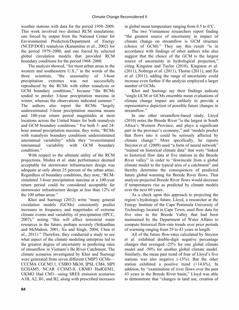
Climate Change Reconsidered II
84
weather stations with data for the period 1950–2009. This work involved two distinct RCM simulations: one forced by output from the National Center for Environmental Prediction/Department of Energy (NCEP/DOE) reanalysis (Kanamitsu et al., 2002) for the period 1979–2000, and one forced by selected global circulation models that provided RCM boundary conditions for the period 1968–2000.
The analysis showed, “for most urban areas in the western and southeastern U.S.,” in the words of the three scientists, “the seasonality of 3-hour precipitation extremes was not successfully reproduced by the RCMs with either reanalysis or GCM boundary conditions,” because “the RCMs tended to predict 3-hour precipitation maxima in winter, whereas the observations indicated summer.” The authors also report the RCMs “largely underestimated 3-hour precipitation maxima means and 100-year return period magnitudes at most locations across the United States for both reanalysis and GCM boundary conditions.” For both 3- and 24-hour annual precipitation maxima, they write, “RCMs with reanalysis boundary conditions underestimated interannual variability” while they “overestimated interannual variability with GCM boundary conditions.”
With respect to the ultimate utility of the RCM projections, Mishra et al. state performance deemed acceptable for stormwater infrastructure design was adequate at only about 25 percent of the urban areas. Regardless of boundary conditions, they note, “RCM-simulated 3-hour precipitation maxima at a 100-year return period could be considered acceptable for stormwater infrastructure design at less than 12% of the 100 urban areas.”
Khoi and Suetsugi (2012) write “many general circulation models (GCMs) consistently predict increases in frequency and magnitudes of extreme climate events and variability of precipitation (IPCC, 2007),” noting “this will affect terrestrial water resources in the future, perhaps severely (Srikanthan and McMahon, 2001; Xu and Singh, 2004; Chen et al., 2011).” Therefore, they conducted a study to see what aspect of the climate modeling enterprise led to the greatest degree of uncertainty in predicting rates of streamflow in Vietnam’s Be River Catchment. The climate scenarios investigated by Khoi and Suetsugi were generated from seven different CMIP3 GCMs—CCCMA CGCM3.1, CSIRO Mk30, IPSL CM4, MPI ECHAM5, NCAR CCSM3.0, UKMO HadGEM1, UKMO Had CM3—using SRES emission scenarios A1B, A2, B1, and B2, along with prescribed increases
in global mean temperature ranging from 0.5 to 6°C. The two Vietnamese researchers report finding
“the greatest source of uncertainty in impact of climate change on streamflow is GCM structure (choice of GCM).” They say this result “is in accordance with findings of other authors who also suggest that the choice of the GCM is the largest source of uncertainty in hydrological projection,” citing Kingston and Taylor (2010), Kingston et al. (2011), Nobrega et al. (2011), Thorne (2011), and Xu et al. (2011), adding the range of uncertainty could increase even further if the analysis employed a larger number of GCMs.
Khoi and Suetsugi say their findings indicate “single GCM or GCMs ensemble mean evaluations of climate change impact are unlikely to provide a representative depiction of possible future changes in streamflow.”
In one other streamflow-based study, Lloyd (2010) notes the Breede River “is the largest in South Africa’s Western Province, and plays a significant part in the province’s economy,” and “models predict that flows into it could be seriously affected by climate change.” More specifically, he reports Steynor et al. (2009) used “a form of neural network” “trained on historical climate data” that were “linked to historical flow data at five stations in the Breede River valley” in order to “downscale from a global climate model to the typical area of a catchment” and thereby determine the consequences of predicted future global warming for Breede River flows. That analysis projected Breede River flows would decrease if temperatures rise as predicted by climate models over the next 60 years.
As a check upon this approach to projecting the region’s hydrologic future, Lloyd, a researcher at the Energy Institute of the Cape Peninsula University of Technology located in Cape Town, used flow data for five sites in the Breede Valley that had been maintained by the Department of Water Affairs to compute historical flow-rate trends over prior periods of warming ranging from 29 to 43 years in length.
All of the future flow-rates calculated by Steynor et al. exhibited double-digit negative percentage changes that averaged -25% for one global climate model and -50% for another global climate model. Similarly, the mean past trend of four of Lloyd’s five stations was also negative (-13%). But the other station exhibited a positive trend (+14.6%). In addition, by “examination of river flows over the past 43 years in the Breede River basin,” Lloyd was able to demonstrate that “changes in land use, creation of
Global Climate Models and Their Limitations
85
impoundments, and increasing abstraction have primarily been responsible for changes in the observed flows” of the negative-trend stations.
Interestingly, Steynor et al. had presumed warming would lead to decreased flow rates, as their projections suggested, and they thus assumed their projections were correct. Lloyd was able to demonstrate those results were driven primarily by unaccounted-for land use changes in the five catchments, and that in his newer study the one site with “a pristine watershed” was the one that had the “14% increase in flow over the study period,” which was “contrary to the climate change predictions” and indicative of the fact that “climate change models cannot yet account for local climate change effects.” Lloyd concludes “predictions of possible adverse local impacts from global climate change should therefore be treated with the greatest caution” and, “above all, they must not form the basis for any policy decisions until such time as they can reproduce known climatic effects satisfactorily.”
Van Haren et al. (2013) write “estimates of future changes in extremes of multi-day precipitation sums are critical for estimates of future discharge extremes of large river basins and changes in [the] frequency of major flooding events,” citing Kew et al. (2010). They indicate “a correct representation of past changes is an important condition to have confidence in projections for the future.”
In an attempt to achieve some of that all-important confidence, van Haren et al. investigated changes in multi-day precipitation extremes in late winter in Europe and the Rhine river basin over the past 60 years using daily precipitation data and “the state-of-the-art gridded high resolution (0.5°) precipitation fields of the European ENSEMBLES project version 7.0 (Haylock et al. 2008),” where “observations [were] averaged to the same regular 1.5° grid when compared directly with the model results.”
The four researchers report the climate models “underestimate the trend in extreme precipitation in the northern half of Europe” because they “underestimate the change in circulation over the past century and as a result have a much smaller (extreme) precipitation response.” More specifically, they state “a dipole in the sea-level pressure trend over continental Europe causes positive trends in extremes in northern Europe and negative trends in the Iberian Peninsula,” while “climate models have a much weaker pressure trend dipole and as a result a much weaker (extreme) precipitation response.”
Van Haren et al. conclude their report by declaring “it is important that we improve our understanding of circulation changes, in particular related to the cause of the apparent mismatch between observed and modeled circulation trends over the past century,” citing Haarsma et al. (2013). References Allan, R.P. and Soden, B.J. 2008. Atmospheric warming and the amplification of precipitation extremes. Science 321: 1481–1484.
Chen, M., Pollard, D., and Barron, E.J. 2003. Comparison of future climate change over North America simulated by two regional climate models. Journal of Geophysical Research 108: 4348–4367.
Dai, A. 2006. Precipitation characteristics in eighteen coupled climate models. Journal of Climate 19: 4605–4630.
Dai, A. and Trenberth, K.E. 2004. The diurnal cycle and its depiction in the Community Climate System Model. Journal of Climate 17: 930–951.
Duffy, P.B., Arritt, R.W., Coquard, J., Gutowski, W., Han, J., Iorio, J., Kim, J., Leung, L.-R., Roads, J., and Zeledon, E. 2006. Simulations of present and future climates in the western United States with four nested regional climate models. Journal of Climate 19: 873–895.
Grimm, N.B., Faeth, S.H., Golubiewski, N.E., Redman, C.L., Wu, J., Bai, X., and Briggs, J.M. 2008. Global change and the ecology of cities. Science 319: 756–760.
Haarsma, R., Selten, F., and van Oldenborgh, G. 2013. Anthropogenic changes of the thermal and zonal flow structure over Western Europe and Eastern North Atlantic in CMIP3 and CMIP5 models. Climate Dynamics 10.1007/s00382-013-1734-8.
Haynes, J.M., L’Ecuyer, T.S., Stephens, G.L., Miller, S.D., Mitrescu, C., Wood, N.B., and Tanelli, S. 2009. Rainfall retrieval over the ocean with spaceborne W-band radar. Journal of Geophysical Research 114: 10.1029/ 2008JD009973.
Haylock, M.R., Hofstra, N., Tank, A.M.G.K., Klok, E.J., Jones, P.D., and New, M. 2008. A European daily high-resolution gridded data set of surface temperature and precipitation for 1950–2006. Journal of Geophysical Research 113: 10.1029/2008JD010201.
Kanamitsu, M., Ebisuzaki, W., Woollen, J., Yang, S.K., Hnilo, J., Fiorino, M., and Potter, G. 2002. NCEP-DOE AMIP-II reanalysis (R-2). Bulletin of the American Meteorological Society 83: 1631–1643.
Climate Change Reconsidered II
86
Kew, S.F., Selten, F.M., Lenderink, G., and Hazeleger, W. 2010. Robust assessment of future changes in extreme precipitation over the Rhine basin using a GCM. Hydrology and Earth Systems Science Discussions 7: 9043–9066.
Kharin, W., Zwiers, F.W., Zhang, X., and Hegerl, G.C. 2007. Changes in temperature and precipitation extremes in the IPCC ensemble of global coupled model simulations. Journal of Climate 20: 1419–1444.
Khoi, D.N. and Suetsugi, T. 2012. Uncertainty in climate change impacts on streamflow in Be River Catchment, Vietnam. Water and Environment Journal 26: 530–539.
Kiktev, D., Caesar, J., Alexander, L.V., Shiogama, H., and Collier, M. 2007. Comparison of observed and multimodeled trends in annual extremes of temperature and precipitation. Geophysical Research Letters 34: 10.1029/ 2007GL029539.
Kim, J. 2005. A projection of the effects of the climate change induced by increased CO2 on extreme hydrologic events in the western U.S. Climatic Change 68: 153–168.
Kingston, D.G. and Taylor, R.G. 2010. Sources of uncertainty in climate change impacts on river discharge and groundwater in a headwater catchment of the Upper Nile Basin, Uganda. Hydrology and Earth System Sciences 14: 1297–1308.
Kingston, D.G., Thompson, J.R., and Kite, G. 2011. Uncertainty in climate change projections of discharge for Mekong River Basin. Hydrology and Earth System Sciences 15: 1459–1471.
Lim, W.H. and Roderick, M.L. 2009. An atlas of the global water cycle. http://epress.anu.edu.au?p=127241
Lloyd, P. 2010. Historical trends in the flows of the Breede River. Water SA 36: 329–333.
Martine, G. et al. 2007. State of World Population 2007: Unleashing the Potential of Urban Growth. United Nations Population Fund, New York, NY, USA.
Mass, C., Skalenakis, A., and Warner, M. 2011. Extreme precipitation over the west coast of North America: Is there a trend? Journal of Hydrometeorology 12: 310–318.
Mearns, L.O., Gutowski, W., Jones, R., Leung, R., McGinnis, S., Nunes, A., and Qian, Y. 2009. A regional climate change assessment program for North America. EOS: Transactions, American Geophysical Union 90: 311.
Milly, P.C.D., Betancourt, J., Falkenmark, M., Hirsch, R.M., Kundzewicz, Z.W., Lettenmaier, D.P., and Stouffer, R.J. 2008. Stationarity is dead: Whither water management? Science 319: 573–574.
Mishra, V., Dominguez, F., and Lettenmaier, D.P. 2012.
Urban precipitation extremes: How reliable are regional climate models? Geophysical Research Letters 39: 10.1029/2011GL050658.
Nobrega, M.T., Collischonn, W., Tucci, C.E.M., and Paz, A.R. 2011. Uncertainty in climate change impacts on water resources in the Rio Grande Basin, Brazil. Hydrology and Earth System Sciences 15: 585–595.
O’Gorman, P.A. and Schneider, T. 2009. The physical basis for increases in precipitation extremes in simulations of 21st-century climate change. Proceedings of the National Academy of Sciences, USA 106: 14,773–14,777.
Rossow, W.B., Mekonnen, A., Pearl, C., and Goncalves, W. 2013. Tropical precipitation extremes. Journal of Climate 26: 1457–1466.
Schliep, E.M., Cooley, D., Sain, S.R., and Hoeting, J.A. 2010. A comparison study of extreme precipitation from six different regional climate models via spatial hierarchical modeling. Extremes 13: 219–239.
Srikanthan, R. and McMahon, T.A. 2001. Stochastic generation of annual, monthly and daily climate data: A review. Hydrology and Earth System Sciences 5: 653–670.
Steynor, A.C., Hewitson, B.C., and Tadross, M.A. 2009. Projected future runoff of the Breede River under climate change. Water SA 35: 433–440.
Stephens, G.L., L’Ecuyer, T., Forbes, R., Gettlemen, A., Golaz, J.-C., Bodas-Salcedo, A., Suzuki, K., Gabriel, P., and Haynes, J. 2010. Dreary state of precipitation in global models. Journal of Geophysical Research 115: 10.1029/ 2010JD014532.
Sun, Y., Solomon, S., Dai, A., and Portmann, R.W. 2006. How often does it rain? Journal of Climate 19: 916–934.
Tebaldi, C., Hayhoe, K., Arblaster, J.M., and Meehl, G.A. 2006. Going to the extremes: An intercomparison of model-simulated historical and future changes in extreme events. Climatic Change 79: 185–211.
Thorne, R. 2011. Uncertainty in the impacts of projected climate change on the hydrology of a subarctic environment: Laird River Basin. Hydrology and Earth System Sciences 15: 1483–1492.
Van Haren, R., van Oldenborgh, G.J., Lenderink, G., and Hazeleger, W. 2013. Evaluation of modeled changes in extreme precipitation in Europe and the Rhine basin. Environmental Research Letters 8: 10.1088/1748–9326/8/1/014053.
Walsh, K. and Pittock, A.B. 1998. Potential changes in tropical storms, hurricanes, and extreme rainfall events as a result of climate change. Climatic Change 39: 199–213.
Wilcox, E.M. and Donner, L.J. 2007. The frequency of
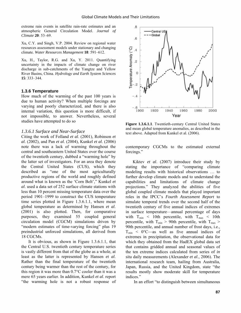
Global Climate Models and Their Limitations
87
extreme rain events in satellite rain-rate estimates and an atmospheric General Circulation Model. Journal of Climate 20: 53–69.
Xu, C.Y. and Singh, V.P. 2004. Review on regional water resources assessment models under stationary and changing climate. Water Resources Management 18: 591–612.
Xu, H., Taylor, R.G. and Xu, Y. 2011. Quantifying uncertainty in the impacts of climate change on river discharge in sub-catchments of the Yangtze and Yellow River Basins, China. Hydrology and Earth System Sciences 15: 333–344.
1.3.6 Temperature How much of the warming of the past 100 years is due to human activity? When multiple forcings are varying and poorly characterized, and there is also internal variation, this question is more difficult, if not impossible, to answer. Nevertheless, several studies have attempted to do so 1.3.6.1 Surface and Near-Surface Citing the work of Folland et al. (2001), Robinson et al. (2002), and Pan et al. (2004), Kunkel et al. (2006) note there was a lack of warming throughout the central and southeastern United States over the course of the twentieth century, dubbed a “warming hole” by the latter set of investigators. For an area they denote the Central United States (CUS), which they described as “one of the most agriculturally productive regions of the world and roughly defined around what is known as the ‘Corn Belt’,” Kunkel et al. used a data set of 252 surface climate stations with less than 10 percent missing temperature data over the period 1901–1999 to construct the CUS temperature time series plotted in Figure 1.3.6.1.1, where mean global temperature as determined by Hansen et al. (2001) is also plotted. Then, for comparative purposes, they examined 55 coupled general circulation model (CGCM) simulations driven by “modern estimates of time-varying forcing” plus 19 preindustrial unforced simulations, all derived from 18 CGCMs.
It is obvious, as shown in Figure 1.3.6.1.1, that the Central U.S. twentieth century temperature series is vastly different from that of the globe as a whole, at least as the latter is represented by Hansen et al. Rather than the final temperature of the twentieth century being warmer than the rest of the century, for this region it was more than 0.7°C cooler than it was a mere 65 years earlier. In addition, Kunkel et al. report “the warming hole is not a robust response of
contemporary CGCMs to the estimated external forcings.”
Kiktev et al. (2007) introduce their study by
stating the importance of “comparing climate modeling results with historical observations … to further develop climate models and to understand the capabilities and limitations of climate change projections.” They analyzed the abilities of five global coupled climate models that played important roles in the IPCC’s Fourth Assessment Report to simulate temporal trends over the second half of the twentieth century of five annual indices of extremes in surface temperature—annual percentage of days with Tmin < 10th percentile, with Tmax < 10th percentile, with Tmin > 90th percentile, with Tmax > 90th percentile, and annual number of frost days, i.e., Tmin < 0°C—as well as five annual indices of extremes in precipitation, the observational data for which they obtained from the HadEX global data set that contains gridded annual and seasonal values of the ten extreme indices calculated from series of in situ daily measurements (Alexander et al., 2006). The international research team, hailing from Australia, Japan, Russia, and the United Kingdom, state “the results mostly show moderate skill for temperature indices.”
In an effort “to distinguish between simultaneous
Figure 1.3.6.1.1. Twentieth-century Central United States and mean global temperature anomalies, as described in the text above. Adapted from Kunkel et al. (2006).
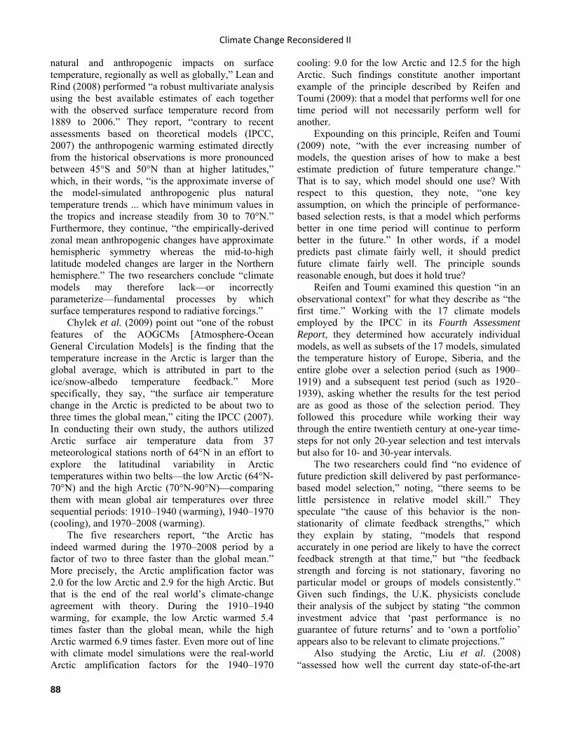
Climate Change Reconsidered II
88
natural and anthropogenic impacts on surface temperature, regionally as well as globally,” Lean and Rind (2008) performed “a robust multivariate analysis using the best available estimates of each together with the observed surface temperature record from 1889 to 2006.” They report, “contrary to recent assessments based on theoretical models (IPCC, 2007) the anthropogenic warming estimated directly from the historical observations is more pronounced between 45°S and 50°N than at higher latitudes,” which, in their words, “is the approximate inverse of the model-simulated anthropogenic plus natural temperature trends ... which have minimum values in the tropics and increase steadily from 30 to 70°N.” Furthermore, they continue, “the empirically-derived zonal mean anthropogenic changes have approximate hemispheric symmetry whereas the mid-to-high latitude modeled changes are larger in the Northern hemisphere.” The two researchers conclude “climate models may therefore lack—or incorrectly parameterize—fundamental processes by which surface temperatures respond to radiative forcings.”
Chylek et al. (2009) point out “one of the robust features of the AOGCMs [Atmosphere-Ocean General Circulation Models] is the finding that the temperature increase in the Arctic is larger than the global average, which is attributed in part to the ice/snow-albedo temperature feedback.” More specifically, they say, “the surface air temperature change in the Arctic is predicted to be about two to three times the global mean,” citing the IPCC (2007). In conducting their own study, the authors utilized Arctic surface air temperature data from 37 meteorological stations north of 64°N in an effort to explore the latitudinal variability in Arctic temperatures within two belts—the low Arctic (64°N-70°N) and the high Arctic (70°N-90°N)—comparing them with mean global air temperatures over three sequential periods: 1910–1940 (warming), 1940–1970 (cooling), and 1970–2008 (warming).
The five researchers report, “the Arctic has indeed warmed during the 1970–2008 period by a factor of two to three faster than the global mean.” More precisely, the Arctic amplification factor was 2.0 for the low Arctic and 2.9 for the high Arctic. But that is the end of the real world’s climate-change agreement with theory. During the 1910–1940 warming, for example, the low Arctic warmed 5.4 times faster than the global mean, while the high Arctic warmed 6.9 times faster. Even more out of line with climate model simulations were the real-world Arctic amplification factors for the 1940–1970
cooling: 9.0 for the low Arctic and 12.5 for the high Arctic. Such findings constitute another important example of the principle described by Reifen and Toumi (2009): that a model that performs well for one time period will not necessarily perform well for another.
Expounding on this principle, Reifen and Toumi (2009) note, “with the ever increasing number of models, the question arises of how to make a best estimate prediction of future temperature change.” That is to say, which model should one use? With respect to this question, they note, “one key assumption, on which the principle of performance-based selection rests, is that a model which performs better in one time period will continue to perform better in the future.” In other words, if a model predicts past climate fairly well, it should predict future climate fairly well. The principle sounds reasonable enough, but does it hold true?
Reifen and Toumi examined this question “in an observational context” for what they describe as “the first time.” Working with the 17 climate models employed by the IPCC in its Fourth Assessment Report, they determined how accurately individual models, as well as subsets of the 17 models, simulated the temperature history of Europe, Siberia, and the entire globe over a selection period (such as 1900–1919) and a subsequent test period (such as 1920–1939), asking whether the results for the test period are as good as those of the selection period. They followed this procedure while working their way through the entire twentieth century at one-year time-steps for not only 20-year selection and test intervals but also for 10- and 30-year intervals.
The two researchers could find “no evidence of future prediction skill delivered by past performance-based model selection,” noting, “there seems to be little persistence in relative model skill.” They speculate “the cause of this behavior is the non-stationarity of climate feedback strengths,” which they explain by stating, “models that respond accurately in one period are likely to have the correct feedback strength at that time,” but “the feedback strength and forcing is not stationary, favoring no particular model or groups of models consistently.” Given such findings, the U.K. physicists conclude their analysis of the subject by stating “the common investment advice that ‘past performance is no guarantee of future returns’ and to ‘own a portfolio’ appears also to be relevant to climate projections.”
Also studying the Arctic, Liu et al. (2008) “assessed how well the current day state-of-the-art

Global Climate Models and Their Limitations
89
reanalyses and CGCMs [coupled global climate models] are reproducing the annual mean, seasonal cycle, variability and trend of the observed SAT [surface air temperature] over the Arctic Ocean for the late twentieth century (where sea ice changes are largest).” The results indicate “large uncertainties are still found in simulating the climate of the twentieth century,” they write, and on an annual basis, “almost two thirds of the IPCC AR4 models have biases that [are] greater than the standard deviation of the observed SAT variability.” Liu et al. further note the models “cannot capture the observed dominant SAT mode variability in winter and seasonality of SAT trends.” The majority of the models “show an out-of-phase relationship between the sea ice area and SAT biases,” they write, and “there is no obvious improvement since the IPCC Third Assessment Report.”
Anagnostopoulos et al. (2010) evaluate the ability of models used by the IPCC to generate regional climates to reproduce observed climate and climate change, and they take issue with the IPCC’s assessment of its models. They compare the output of these models to temperature and precipitation observations at 55 points worldwide. They then do a similar comparison for 70 points in the USA on several time scales. They selected the USA for the refined study because it has a dense network of surface stations. Thus, they can evaluate the model performance at the large scale and the regional scale.
In order to compare observed records to model projections, they use a statistical technique called “best linear unbiased estimation,” comparing observations at a particular station and nearby stations to a linear combination of the model outputs and comparing the time series via traditional statistical measures.
The authors demonstrate, “At the monthly time scale the models generally reproduce the sequence of cold-warm and wet-dry periods at all stations examined.” However, the results were much worse at the annual time scale and the variability in the general circulation is underestimated. For the climate time-scales, some of the grid points will show 30-year temperature rises in the model simulation, but the actual data shows temperature falls. This is similar for both the large and regional scales. Additionally, the models could not capture the long-term climate changes from 1890 to the end of the twentieth century at many of the points (Figure 1.3.6.2).
As Anagnostopoulos et al. state, “It is claimed that GCMs provide credible quantitative estimates of future climate change, particularly at continental times scales and above. Examining the local performance of the models at 55 points, we found that local projections do not correlate well with observed measurements.” They found the model performance was actually worse on larger scales than on regional ones. They suggest the central issue is not about the performance of the GCMs, but whether climate can be predicted deterministically at all given the uncertainties inherent in the atmosphere.
Anagnostopoulos et al. use statistics to make the point others have made regarding models using dynamics. Anagnostopoulos et al. say there simply may not be a predictable “core” to the climate that is only obscured by layers of complexity or uncertainty. They also propose a shift in our modeling approach, suggesting statistical methods, in addition to dynamical methods and models, be used to generate future scenarios for climate as has been done successfully in other fields such as thermophysics or turbulence.
Lo and Hsu (2010) point out “widespread abrupt warming in the extratropical Northern Hemisphere occurred in the late 1980s” and say the warming was associated with a change in the relative influence of a
Figure 1.3.6.1.2. The observed and model temperature time series integrated over the USA (annual means and maximum and minimum monthly) for the annual and 30-year time scales. Adapted from Figure 12 in Anagnostopoulos et al. (2010).

Climate Change Reconsidered II
90
Pacific Decadal Oscillation (PDO)-like pattern and an Arctic Oscillation (AO)-like pattern. Utilizing land surface temperature data obtained from the University of East Anglia’s Climatic Research Unit (Mitchell et al., 2004), plus sea surface temperature data obtained from the U.K.’s Meteorological Office (Rayner et al., 2003), the authors explored the nature of this temperature increase and tested the ability of IPCC/CMIP3 models to simulate it.
The two Taiwanese researchers report the “accelerated warming in the Northern Hemisphere” was related to the emergence of an AO-like pattern in the late 1980s and the concomitant weakening of the previously prevailing PDO-like pattern occurring in tandem. These resultsthey say, , together with results obtained from current IPCC/CMIP3 models, “do not support the scenario that the emerging influence of the AO-like pattern in the 1980s can be attributed to the anthropogenic greenhouse effect.” Lo and Hsu also conclude, “this study indicates the importance of the changing behavior of the decadal fluctuations in the recent climate regime shift,” and they highlight what they call “the insufficient capability of the present state-of-the-art IPCC/CMIP3 models in simulating this change.”
DelSole et al. (2011) used a set of climate models run in “control” or unforced mode to develop a 300-year data set of spatial ocean temperature data, where it was found that an internal pattern, detectable using a spatial fingerprinting technique, could be identified in the simulated data. This spatial pattern of ocean temperature anomalies was labeled the Internal Multidecadal Pattern (IMP). It was found to be highly coherent with the Atlantic Multidecadal Oscillation (AMO), suggesting the models were able to match the internal dynamics of the real-Earth system reasonably well. The researchers next extracted, also by means of discriminant fingerprinting, the forced component of the spatial patterns produced in the absence of the IMP as an orthogonal function, which they demonstrated has only a minor effect (less than 1/7 the amplitude) on the IMP. They then used historical sea surface temperature data to evaluate the relative importance of the forced vs. IMP components of change since 1850.
In considering the latter portion of the record (1946–2008), the results indicate the internal variability component of climate change (the IMP) operated in a cooling mode between 1946 and 1977, but switched thereafter to a warming mode between 1977 and 2008, suggesting the IMP is strong enough to overwhelm any anthropogenic signal during this
latter period of time. They also note “the trend due to only the forced component is statistically the same in the two 32-year periods and in the 63-year period.” That is to say, the forced part was not accelerating. Taken together, these results imply the observed trend differs between the periods 1946–1977 and 1977–2008 not because the forced response accelerated but because “internal variability led to relative cooling in the earlier period and relative warming in the later period.” Their results suggest simple extrapolations of rates of warming from 1980 onward overestimate the forced component of warming, and therefore using this period without factoring out internal variability will likely lead to unrealistic values of climate sensitivity.
Lavers et al. (2009), in a study described previously in Section 1.4.5.1, assessed the predictability of monthly “retrospective forecasts,” or hindcasts, composed of multiple nine-month projections initialized during each month of the year over the period 1981–2001, comparing the projections against real-world air temperatures obtained from ERA-40 reanalysis data. In addition, they conducted a virtual-world analysis where the output of one of the models was arbitrarily assumed to be the truth and the average of the rest of the models was assumed to be the predictor.
The researchers report that in the virtual world of the climate models, there was quite good skill over the first two weeks of the forecast, when the spread of ensemble model members was small, but there was a large drop-off in predictive skill in the second 15-day period. Things were worse in the real world, where they say the models had negligible skill over land at a 31-day lead time, “a relatively short lead time in terms of seasonal climate prediction.” The three researchers conclude, “it appears that only through significant model improvements can useful long-lead forecasts be provided that would be useful for decision makers,” a quest they state “may prove to be elusive.”
Crook and Forster (2011) note “predicting our future influence on climate requires us to have confidence in the climate models used to make predictions, and in particular that the models’ climate sensitivity and ocean heat storage characteristics are realistic.” They go on to say that confidence may be gained “by assessing how well climate models reproduce current climatology and climate variability, and how their feedback parameters compare with estimates from observations.”
Using the World Climate Research Programme’s

Global Climate Models and Their Limitations
91
Coupled Model Intercomparison Project phase 3 (CMIP3) and real-world data from the HadCRUT3 database, Crook and Forster first determined “the surface temperature response contributions due to long-term radiative feedbacks, atmosphere-adjusted forcing, and heat storage and transport for a number of coupled ocean-atmosphere climate models,” after which they compared “the linear trends of global mean, Arctic mean and tropical mean surface temperature responses of these models with observations over several time periods.” They also investigated “why models do or do not reproduce the observed temperature response patterns” and performed “optimal fingerprinting analyses on the components of surface temperature response to test their forcing, feedback and heat storage responses.”
The two University of Leeds (U.K.) researchers found tropical twentieth century warming was too large and Arctic amplification too low in the Geophysical Fluid Dynamics Laboratory CM2.1 model, the Meteorological Research Institute CGCM232a model, and the MIROC3(hires) model “because of unrealistic forcing distributions.” They also determined “the Arctic amplification in both National Center for Atmospheric Research models is unrealistically high because of high feedback contributions in the Arctic compared to the tropics.” In addition, they report, “few models reproduce the strong observed warming trend from 1918 to 1940,” noting “the simulated trend is too low, particularly in the tropics, even allowing for internal variability, suggesting there is too little positive forcing or too much negative forcing in the models at this time.”
According to Miao et al. (2012), the accuracy of any GCM “should be established through validation studies before using it to predict future climate scenarios.” “Although accurate simulation of the present climate does not guarantee that forecasts of future climate will be reliable,” they write, “it is generally accepted that the agreement of model predictions with present observations is a necessary prerequisite in order to have confidence in the quality of a model.”
Working within this conceptual framework, Miao et al. assessed the performance of the AR4 GCMs, otherwise known as the CMIP3 models, in simulating precipitation and temperature in China from 1960 to 1999, comparing the model simulations with observed data using “system bias (B), root-mean-square error (RMSE), Pearson correlation coefficient (R) and Nash-Sutcliffe model efficiency (E)” as evaluation metrics.
The four researchers find certain of the CMIP3 models “are unsuitable for application to China, with little capacity to simulate the spatial variations in climate across the country,” adding that all of them “give unsatisfactory simulations of the inter-annual temporal variability.” In addition, they find “each AR4 GCM performs differently in different regions of China.” Miao et al. conclude “the inter-annual simulations (temperature and precipitation) by AR4 GCMs are not suitable for direct application” and “caution should be applied when using outputs from the AR4 GCMs in hydrological and ecological assessments” due to their “poor performance.”
According to Morak et al. (2013), studies of observational temperature records over the past 50 to 100 years have found evidence for increases in both mean and extreme (maximum and minimum) near-surface air temperatures, but they note the increase in maximum temperature has been of smaller magnitude than the increase in minimum temperature. This state of affairs has led to a decrease in the diurnal temperature range. They compared “observed and climate model-simulated trends in mean values of temperature extreme indices, splitting the year into the dynamically active boreal cold (ONDJFM) and warm (AMJJAS) seasons.” To do so, they used “modeled daily minimum and maximum surface temperature data derived from simulations with the Hadley Centre Global Environmental Model, version 1 (HadGEM1).”
The three U.K. researchers report, among other findings, that the model “significantly underestimates changes in some regions, particularly in winter across large parts of Asia” and “has a tendency to overestimate changes in the frequency of hot days in both the [a] winter and [b] summer seasons over [d] most regions, and in the [e] global and [f] hemispheric mean.” The model “also overestimates changes in the frequency of warm winter days on larger scales.” With respect to changes in cold extremes the model “does underestimate them in some regions” and “there are some regions with trends of the opposite sign.” In addition, Morak et al. “the particular regional trend pattern, often also referred to as the ‘warming hole,’ is not evident in the simulated trend pattern,” citing Pan et al. (2004), Kunkel et al. (2006), Portmann et al. (2009), and Meehl et al. (2012). And they say “the model shows a tendency to significantly overestimate changes in warm daytime extremes, particularly in summer.” Although the HadGEM1 does some things well, there are a number of other things it has yet to accomplish

Climate Change Reconsidered II
92
satisfactorily. As the observed rate of rise in the global average
temperature has slowed during recent decades, the gap between observations and climate models results has widened. The discrepancy is now so large as to indicate a statistically significant difference between the climate modeled trends and the observed trend. The existence of such a large discrepancy is a strong indication that climate models are failing in their ability to accurately capture known changes in this key parameter of Earth’s climate system.
A clear demonstration the models are failing to contain observations was made by Knappenberger and Michaels (2013), who compiled the range of trends in surface temperatures during the first several decades of the twenty-first century projected by CMIP3 climate models running emissions scenario A1B. Knappenberger and Michaels placed the observed temperatures within this modeled distribution (see Figure 1.3.6.1.3). The observed trends lie very close to, and in some cases below, the lower bound of the 95% certainty range derived from climate model projections. Knappenberger and Michaels report “at the global scale, climate models are on the verge of failing to adequately capture observed changes in the average temperature over the past 10 to 30 years—the period of the greatest human influence on the atmosphere.” They conclude, “It is
impossible to present reliable future projections from a collection of climate models which generally cannot simulate observed change.”
In the same vein, Fyfe et al. (2013) examined the performance of the newer CMIP5 climate models and found a similar result. The researchers “considered trends in global mean surface temperature computed from 117 simulations of the climate by 37 CMIP5 models.” They note the “models generally simulate natural variability—including that associated with the El Niño–Southern Oscillation and explosive volcanic eruptions—as well as estimate the combined response of climate to changes in greenhouse gas concentrations, aerosol abundance (of sulphate, black carbon and organic carbon, for example), ozone concentrations (tropospheric and stratospheric), land use (for example, deforestation) and solar variability.” But despite the models’ claimed ability to simulate both natural variability and human influences, when compared against actual observations, their simulation of the evolution of the global average temperature is flawed. Over the past 20 years (1993–2012), Fyfe et al. find the “rate of warming is significantly slower than that simulated by the climate models participating in Phase 5 of the Coupled Model Intercomparison Project (CMIP5)” and “the inconsistency between observed and simulated global warming is even more striking for temperature trends
Figure 1.3.6.1.3. Trends (through 2012) in three observed global surface temperature records of length 5 to 15 years (colored lines) set against the probability (gray lines) derived from the complete collection of climate model runs used in the IPCC Fourth Assessment Report under the SRES A1B emissions scenario. Adapted from Knappenberger and Michaels (2013).
Global Climate Models and Their Limitations
93
computed over the past fifteen years (1998–2012).” They add, “It is worth noting that the observed trend over this period—not significantly different from zero—suggests a temporary ‘hiatus’ in global warming.” Fyfe et al. conclude, “Ultimately the causes of this inconsistency will only be understood after careful comparison of simulated internal climate variability and climate model forcings with observations from the past two decades, and by waiting to see how global temperature responds over the coming decades.”
The IPCC is in a very difficult position. In order to defend the CMIP5 suite of models, it must somehow argue they did not underpredict warming as the greatest increases in atmospheric carbon dioxide content occurred. Further, they must invalidate at least 19 separate experiments authored by 42 researchers in the citations noted earlier in this section. References Alexander, L.V. et al. 2006. Global observed changes in daily climate extremes of temperature and precipitation. Journal of Geophysical Research 111: 10.1029/ 2005JD006290.
Anagnostopoulos, G.G., Koutsoyiannis, D., Christofides, A., Efstradiadis, A., and Mamassis, N. 2010. A comparison of local and aggregated climate model outputs with observed data. Hydrological Sciences Journal 55: 1094–1110.
Chylek, P., Folland, C.K., Lesins, G., Dubey, M.K., and Wang, M. 2009. Arctic air temperature change amplification and the Atlantic Multidecadal Oscillation. Geophysical Research Letters 36: 10.1029/2009GL038777.
Crook, J.A. and Forster, P.M. 2011. A balance between radiative forcing and climate feedback in the modeled 20th century temperature response. Journal of Geophysical Research 116: 10.1029/2011JD015924.
DelSole, T., Tippett, M.K., and Shukla, J. 2011. A significant component of unforced multidecadal variability in the recent acceleration of global warming. Journal of Climate 24: 909–926.
Folland, C.K. et al. 2001. Observed climate variability and change. In: Houghton, J.T. et al. (Eds.). Climate Change 2001: The Scientific Basis, Cambridge University Press, Cambridge, UK, pp. 99–181.
Fyfe, J.C., Gillett, N.P., and Zwiers, F.W. 2013. Overestimated global warming over the past 20 years. Nature Climate Change 3: 767–769.
Hansen, J., Ruedy, R., Sato, M., Imhoff, M., Lawrence, W., Easterling, D., Peterson, T., and Karl, T. 2001. A closer look at United States and global surface temperature change. Journal of Geophysical Research 106: 23,947–23,963.
Intergovernmental Panel on Climate Change. 2007. Climate Change 2007: The Physical Science Basis, Contribution of Working Group I to the Fourth Assessment Report of the Intergovernmental Panel on Climate Change. Solomon, S. et al. (Eds.) Cambridge University Press, Cambridge, UK.
Kiktev, D., Caesar, J., Alexander, L.V., Shiogama, H., and Collier, M. 2007. Comparison of observed and multimodeled trends in annual extremes of temperature and precipitation. Geophysical Research Letters 34: 10.1029/ 2007GL029539.
Knappenberger, P.C. and Michaels, P.J., 2013. Policy Implications of Climate Models on the Verge of Failure. American Geophysical Union Science Policy Conference. Washington, DC, June 24–26, 2013.
Kunkel, K.E., Liang, X.-Z., Zhu, J., and Lin, Y. 2006. Can CGCMs simulate the twentieth-century “warming hole” in the central United States? Journal of Climate 19: 4137–4153.
Lavers, D., Luo, L., and Wood, E.F. 2009. A multiple model assessment of seasonal climate forecast skill for applications. Geophysical Research Letters 36: 10.1029/ 2009GL041365.
Lean, J.L. and Rind, D.H. 2008. How natural and anthropogenic influences alter global and regional surface temperatures: 1889 to 2006. Geophysical Research Letters 35: 10.1029/2008GL034864.
Liu, J., Zhang, Z., Hu, Y., Chen, L., Dai, Y., and Ren, X. 2008. Assessment of surface air temperature over the Arctic Ocean in reanalysis and IPCC AR4 model simulations with IABP/POLES observations. Journal of Geophysical Research 113: 10.1029/2007JD009380.
Lo, T.-T. and Hsu, H.-H. 2010. Change in the dominant decadal patterns and the late 1980s abrupt warming in the extratropical Northern Hemisphere. Atmospheric Science Letters 11: 210–215.
Meehl, G.A., Arblaster, J.M., and Branstator, G. 2012. Mechanisms contributing to the warming hole and the consequent U.S. east-west differential of heat extremes. Journal of Climate 25: 6394–6408.
Miao, C., Duan, Q., Yang, L., and Borthwick, A.G.L. 2012. On the applicability of temperature and precipitation data from CMIP3 for China. PLoS ONE 7: e44659.
Mitchell, T.D., Carter, T.R., Jones, P.D., Hulme, M., and

Climate Change Reconsidered II
94
New, M. 2004. A comprehensive set of high-resolution grids of monthly climate for Europe and the globe: the observed record (1901-2000) and 16 scenarios (2001–2100). Tyndall Centre Working Paper 55, Norwich, United Kingdom.
Pan, Z., Arritt, R.W., Takle, E.S., Gutowski Jr., W.J., Anderson, C.J., and Segal, M. 2004. Altered hydrologic feedback in a warming climate introduces a “warming hole.” Geophysical Research Letters 31: 10.1029/2004GL 020528.
Portmann, R.W., Solomon, S., and Hegerl, G.C. 2009. Spatial and seasonal patterns in climate change, temperatures, and precipitation across the United States. Proceedings of the National Academy of Sciences 106: 7324–7329.
Rayner, N.A., Parker, D.E., Horton, E.B., Folland, C.K., Alexander, L.V., Rowell, D.P., Kent, E.C., and Kaplan, A. 2003. Global analyses of sea surface temperature, sea ice, and night marine air temperature since the late nineteenth century. Journal of Geophysical Research 35: 10.1029/ 2002JD002670.
Reifen, C. and Toumi, R. 2009. Climate projections: Past performance no guarantee of future skill? Geophysical Research Letters 36: 10.1029/2009GL038082.
Robinson, W.A., Reudy, R., and Hansen, J.E. 2002. On the recent cooling in the east-central United States. Journal of Geophysical Research 107: 10.1029/2001JD001577.
1.4.6.2 Mid- and Upper-Troposphere Several studies have examined model treatment of processes in the troposphere. The testing of climate model results is an important but difficult problem. One of the key model results is the presence of a tropical troposphere “hotspot” in which the troposphere warms faster than the surface under conditions of enhanced greenhouse gas forcing. Previous studies have produced disagreement over whether data were consistent with models on this question. However, Christy et al. (2010) made several advances by doing enhancing the data for surface trends, extending the data to a 31-year length, evaluating the wind-based temperature estimates, and clarifying the meaning of “best estimate” multi-data warming trends from data and models.
Two prior studies had derived tropospheric temperature trends from the Thermal Wind Equation (TWE)—which uses radiosonde measurements of wind speed to calculate temperature—on the theoretical basis that warmer air should move faster than cooler air. They found there were biases in the
data for this type of calculation. For example, particularly for older radiosonde observations, on days when the upper wind was stronger, the balloons would tend to blow out of receiver range. This created a bias by causing missing data for high winds for older observations, leading to a spurious warm trend over time. Overall, the TWE-based trends were three times greater than trends derived from all other types of data. In addition, they did not agree with other wind data and also were based on much sparser data. Radiosonde data were therefore not used in the Christy et al. analysis, which also identified a small warm bias in the RSS satellite data that was explained by Christy and his colleagues.
The next innovation was to use the Scaling Ratio (SR), the ratio of atmospheric temperature trend to surface temperature trend. The SR attempts to factor out the effect of the lack of actual (historic) El Niños or other oscillations in climate model runs, and such simulated events in different computer runs. Christy and his eight colleagues found the SR for real-world data was 0.8 ± 0.3, whereas the model simulations had a SR of 1.38 ± 0.08 (a significant difference). That is, the data show a lower rate of warming for the lower troposphere than for the surface (though not statistically different), whereas the models show amplification. The SR value for the middle troposphere data was 0.4, even more different from the model predictions. Only the SR for RSS data, which has a documented warming bias, overlaps with any model SR results. Given these findings, the work of Christy et al. suggests current state-of-the-art climate models are fundamentally wrong in how they represent this portion of Earth’s atmosphere.
The tropical troposphere also was the focus of study for Fu et al. (2011), who note the IPCC Fourth Assessment Report (AR4) general circulation models “predict a tropical tropospheric warming that increases with height, reaches its maximum at ~200 hPa, and decreases to zero near the tropical tropopause.” They add, “this feature has important implications to the climate sensitivity because of its impact on water vapor, lapse rate and cloud feedbacks and to the change of atmospheric circulations.” Therefore, they write, it is “critically important to observationally test the GCM-simulated maximum warming in the tropical upper troposphere.”
Fu et al. thus examined trends in the temperature difference (ΔT) between the tropical upper- and lower-middle-troposphere based on satellite microwave sounding unit (MSU) data, as interpreted by University of Alabama at Huntsville (UAH) and
Global Climate Models and Their Limitations
95
Remote Sensing System (RSS) teams, comparing both sets of results with AR4 GCM ΔT simulations for the period 1979–2010.
The three researchers report the RSS and UAH ΔT time series “agree well with each other” and showed little trend over the period of record. By contrast, they note there is “a steady positive trend” in the model-simulated ΔT results, concluding the significantly smaller ΔT trends from both the RSS and UAH teams “indicate possible common errors among AR4 GCMs.” In addition, they note the tropical surface temperature trend of the multi-model ensemble mean is more than 60% larger than that derived from observations, “indicating that AR4 GCMs overestimate the warming in the tropics for 1979–2010.”
In addition to greatly overestimating the tropical surface temperature trend, Fu et al. note, “it is evident that the AR4 GCMs exaggerate the increase in static stability between [the] tropical middle and upper troposphere during the last three decades.”
One year later, Po-Chedley and Fu (2012) write, “recent studies of temperature trend amplification in the tropical upper troposphere relative to the lower-middle troposphere found that coupled atmosphere-ocean models from CMIP3 exaggerated this amplification compared to satellite microwave sounding unit (Fu et al., 2011) and radiosonde (Seidel et al., 2012) observations.” The two authors “revisit this issue using atmospheric GCMs with prescribed historical sea surface temperatures (SSTs) and coupled atmosphere-ocean GCMs that participated in the latest model intercomparison project, CMIP5.”
The pair of researchers report their work demonstrated “even with historical SSTs as a boundary condition, most atmospheric models exhibit excessive tropical upper tropospheric warming relative to the lower-middle troposphere as compared with satellite-borne microwave sounding unit measurements.” In addition, they note, “the results from CMIP5 coupled atmosphere-ocean GCMs are similar to findings from CMIP3 coupled GCMs.”
Focusing more on the mid-troposphere, Handorf et al. (2012) write, “atmospheric teleconnections describe important aspects of the low-frequency atmospheric variability on time-scales of months and longer,” adding “in light of the increased need to provide reliable statements about seasonal to decadal predictability, it is necessary that state-of-the-art climate models simulate the spatial and temporal behavior of atmospheric teleconnections satisfactorily.” Therefore, they continue, “an
evaluation of climate models requires the evaluation of the simulated climate variability in terms of teleconnection patterns.” Handorf and Dethloff evaluated “the ability of state-of-the-art climate models to reproduce the low-frequency variability of the mid-tropospheric winter flow of the Northern Hemisphere in terms of atmospheric teleconnection patterns.” To do so, they used the CMIP3 multimodel ensemble for the period 1958–1999, for which reliable reanalysis data were available for comparison.
The two researchers conclude, “current state-of-the-art climate models are not able to reproduce the temporal behavior, in particular the exact phasing of the dominant patterns due to internally generated model variability.” In addition, they write, “the state-of-the-art climate models are not able to capture the observed frequency behavior and characteristic time scales for the coupled runs satisfactorily ... in accordance with Stoner et al. (2009) and Casado and Pastor (2012),” both of which studies conclude, in their words, that “the models are not able to reproduce the temporal characteristics of atmospheric teleconnection time-series.”
“In light of the strong need to provide reliable assessments of decadal predictability,” Handorf and Dethloff additionally state “the potential of atmospheric teleconnections for decadal predictability needs further investigations” that “require a better understanding of [1] the underlying mechanisms of variability patterns and flow regimes, [2] an improvement of the skill of state-of-the-art climate and Earth system models in reproducing atmospheric teleconnections and [3] the identification of sources for long-range predictive skill of teleconnections.”
In other research, Santer et al. (2011) examined the consistency between satellite observations of the lower troposphere and climate model simulations of that atmospheric region. The 17 researchers set the average of the observed temperature trends of lengths varying from 10 to 32 years against the distribution of the same trend as simulated by a collection of CMIP3 climate models (see Figure 1.4.6.2.1). While the lower troposphere temperature trends (TLT) “in the observational satellite datasets are not statistically unusual relative to model-based distributions of externally forced TLT trends” they found “it should be qualified by noting that: 1) The multi-model average TLT trend is always larger than the average observed TLT trend” and “2) As the trend fitting period increases … average observed trends are increasingly more unusual with respect to the multi-
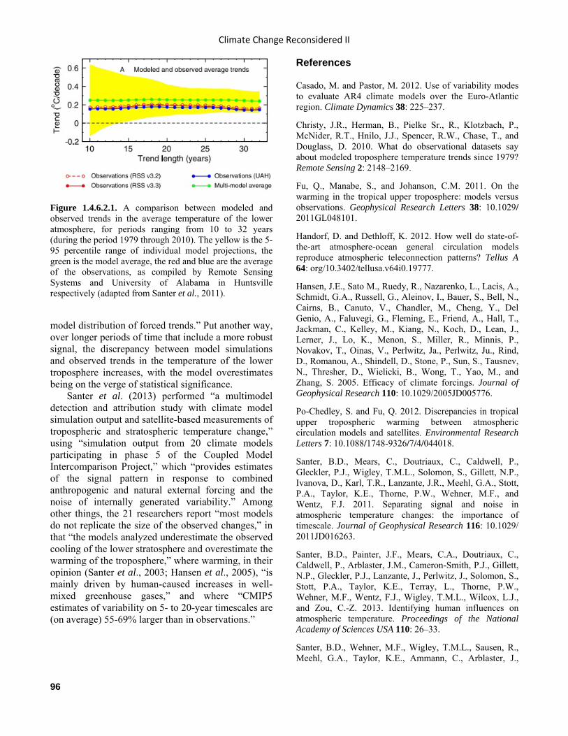
Climate Change Reconsidered II
96
model distribution of forced trends.” Put another way, over longer periods of time that include a more robust signal, the discrepancy between model simulations and observed trends in the temperature of the lower troposphere increases, with the model overestimates being on the verge of statistical significance.
Santer et al. (2013) performed “a multimodel detection and attribution study with climate model simulation output and satellite-based measurements of tropospheric and stratospheric temperature change,” using “simulation output from 20 climate models participating in phase 5 of the Coupled Model Intercomparison Project,” which “provides estimates of the signal pattern in response to combined anthropogenic and natural external forcing and the noise of internally generated variability.” Among other things, the 21 researchers report “most models do not replicate the size of the observed changes,” in that “the models analyzed underestimate the observed cooling of the lower stratosphere and overestimate the warming of the troposphere,” where warming, in their opinion (Santer et al., 2003; Hansen et al., 2005), “is mainly driven by human-caused increases in well-mixed greenhouse gases,” and where “CMIP5 estimates of variability on 5- to 20-year timescales are (on average) 55-69% larger than in observations.”
References Casado, M. and Pastor, M. 2012. Use of variability modes to evaluate AR4 climate models over the Euro-Atlantic region. Climate Dynamics 38: 225–237.
Christy, J.R., Herman, B., Pielke Sr., R., Klotzbach, P., McNider, R.T., Hnilo, J.J., Spencer, R.W., Chase, T., and Douglass, D. 2010. What do observational datasets say about modeled troposphere temperature trends since 1979? Remote Sensing 2: 2148–2169.
Fu, Q., Manabe, S., and Johanson, C.M. 2011. On the warming in the tropical upper troposphere: models versus observations. Geophysical Research Letters 38: 10.1029/ 2011GL048101.
Handorf, D. and Dethloff, K. 2012. How well do state-of-the-art atmosphere-ocean general circulation models reproduce atmospheric teleconnection patterns? Tellus A 64: org/10.3402/tellusa.v64i0.19777.
Hansen, J.E., Sato M., Ruedy, R., Nazarenko, L., Lacis, A., Schmidt, G.A., Russell, G., Aleinov, I., Bauer, S., Bell, N., Cairns, B., Canuto, V., Chandler, M., Cheng, Y., Del Genio, A., Faluvegi, G., Fleming, E., Friend, A., Hall, T., Jackman, C., Kelley, M., Kiang, N., Koch, D., Lean, J., Lerner, J., Lo, K., Menon, S., Miller, R., Minnis, P., Novakov, T., Oinas, V., Perlwitz, Ja., Perlwitz, Ju., Rind, D., Romanou, A., Shindell, D., Stone, P., Sun, S., Tausnev, N., Thresher, D., Wielicki, B., Wong, T., Yao, M., and Zhang, S. 2005. Efficacy of climate forcings. Journal of Geophysical Research 110: 10.1029/2005JD005776.
Po-Chedley, S. and Fu, Q. 2012. Discrepancies in tropical upper tropospheric warming between atmospheric circulation models and satellites. Environmental Research Letters 7: 10.1088/1748-9326/7/4/044018.
Santer, B.D., Mears, C., Doutriaux, C., Caldwell, P., Gleckler, P.J., Wigley, T.M.L., Solomon, S., Gillett, N.P., Ivanova, D., Karl, T.R., Lanzante, J.R., Meehl, G.A., Stott, P.A., Taylor, K.E., Thorne, P.W., Wehner, M.F., and Wentz, F.J. 2011. Separating signal and noise in atmospheric temperature changes: the importance of timescale. Journal of Geophysical Research 116: 10.1029/ 2011JD016263.
Santer, B.D., Painter, J.F., Mears, C.A., Doutriaux, C., Caldwell, P., Arblaster, J.M., Cameron-Smith, P.J., Gillett, N.P., Gleckler, P.J., Lanzante, J., Perlwitz, J., Solomon, S., Stott, P.A., Taylor, K.E., Terray, L., Thorne, P.W., Wehner, M.F., Wentz, F.J., Wigley, T.M.L., Wilcox, L.J., and Zou, C.-Z. 2013. Identifying human influences on atmospheric temperature. Proceedings of the National Academy of Sciences USA 110: 26–33.
Santer, B.D., Wehner, M.F., Wigley, T.M.L., Sausen, R., Meehl, G.A., Taylor, K.E., Ammann, C., Arblaster, J.,
Figure 1.4.6.2.1. A comparison between modeled and observed trends in the average temperature of the lower atmosphere, for periods ranging from 10 to 32 years (during the period 1979 through 2010). The yellow is the 5-95 percentile range of individual model projections, the green is the model average, the red and blue are the average of the observations, as compiled by Remote Sensing Systems and University of Alabama in Huntsville respectively (adapted from Santer et al., 2011).

Global Climate Models and Their Limitations
97
Washington, W.M., Boyle, J.S., and Bruggemann, W. 2003. Contributions of anthropogenic and natural forcing to recent tropopause height changes. Science 301: 479–483.
Seidel, D.J., Free, M., and Wang, J.S. 2012. Reexamining the warming in the tropical upper troposphere: Models versus radiosonde observations. Geophysical Research Letters 39: 10.1029/2012GL053850
Stoner, A.M.K., Hayhoe, K., and Wuebbles, D.J. 2009. Assessing general circulation model simulations of atmospheric teleconnection patterns. Journal of Climate 22: 4348–4372.
1.3.7 Oceans The vast majority of the surface of the planet consists of oceans, which play a significant role in the modulation and control of Earth’s climate. As is true of other factors we have previously discussed, modeling of the oceans has proved to be a difficult task. 1.3.7.1 Atlantic Ocean Keeley et al. (2012) note, “current state-of-the-art climate models fail to capture accurately the path of the Gulf Stream and North Atlantic Current,” and this model failure “leads to a warm bias near the North American coast, where the modeled Gulf Stream separates from the coast further north, and a cold anomaly to the east of the Grand Banks of Newfoundland, where the North Atlantic Current remains too zonal.”
Using a high-resolution coupled atmosphere-ocean model (HiGEM), described in detail by Shaffrey et al. (2009), Keeley et al. analyzed the impacts of the sea surface temperature (SST) biases created by the model in the North Atlantic in winter—approximately 8°C too cold to the east of the Grand Banks of Newfoundland and 6°C too warm near the east coast of North America—on the mean climatic state of the North Atlantic European region, along with the variability associated with those model-induced SST biases.
The three UK researchers say their results indicate the model-induced SST errors produce a mean sea-level pressure response “similar in magnitude and pattern to the atmospheric circulation errors in the coupled climate model.” They also note “errors in the coupled model storm tracks and North Atlantic Oscillation, compared to reanalysis data, can also be explained partly by these SST errors.” Keeley et al. conclude, “both [1] the error in the Gulf Stream separation location and [2] the path of the North
Atlantic Current around the Grand Banks play important roles in affecting the atmospheric circulation”; they further note “reducing these coupled model errors could improve significantly the representation of the large-scale atmospheric circulation of the North Atlantic and European region.” References Keeley, S.P.E., Sutton, R.T., and Shaffrey, L.C. 2012. The impact of North Atlantic sea surface temperature errors on the simulation of North Atlantic European region climate. Quarterly Journal of the Royal Meteorological Society 138: 1774–1783.
Shaffrey, L.C., Stevens, I., Norton, W.A., Roberts, M.J., Vidale, P.L., Harle, J.D., Jrrar, A., Stevens, D.P., Woodage, M.J., Demory, M.E., Donners, J., Clark, D.B., Clayton, A., Cole, J.W., Wilson, S.S., Connolley, W.M., Davies, T.M., Iwi, A.M., Johns, T.C., King, J.C., New, A.L., Slingo, J.M., Slingo, A., Steenman-Clark, L., and Martin, G.M. 2009. U.K. HiGEM: The new U.K. High-Resolution Global Environment Model: model description and basic evaluation. Journal of Climate 22: 1861–1896.
1.3.7.2 Pacific Ocean Thompson and Kwon (2010) used a state-of-the-art coupled-atmosphere-ocean general circulation model known as the Community Climate System Model version 3 (CCSM3) to demonstrate that climate models have difficulty simulating interdecadal variations in the Pacific Ocean Circulation. The authors used the model with atmospheric radiative forcing fixed to 1990 levels and with medium-scale grid resolution. The model output was run for 700 years and a 100-year slice was selected starting with year 500.
The model was unable to capture the natural characteristics of the Kuroshio Current and its extension (KE), resulting in a poor representation of climate variability in the North Pacific region. In nature, the mean position of the KE and the strongest sea surface temperature (SST) gradients are typically separated by 500 km. In the model control run, the two phenomena were coincident, resulting in excessively strong SST variations (Figure 1.3.7.2.1).
The Kuroshio Current, like its Atlantic counterpart, the Gulf Stream, is a strong, narrow current in the Northwest Pacific that runs along Japan and continues into the North Pacific. The Oyashio Extension (OE) is a distinct current running along the Kurile Islands and Hokkaido. This current is
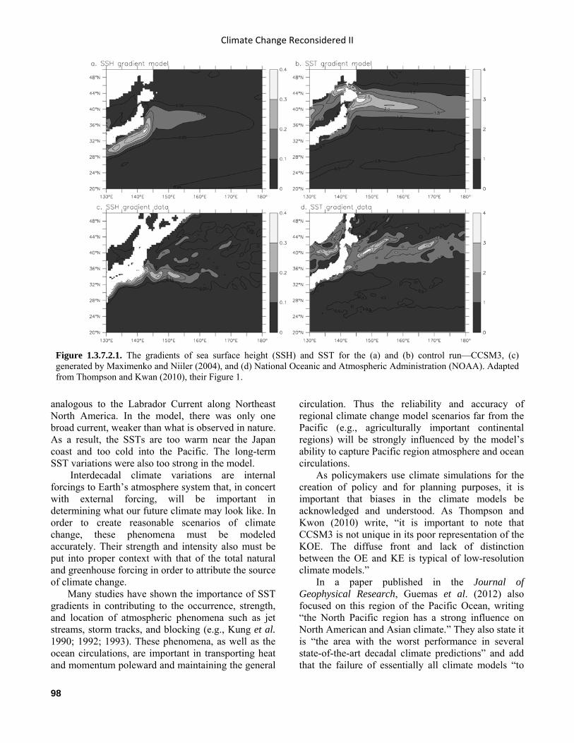
Climate Change Reconsidered II
98
analogous to the Labrador Current along Northeast North America. In the model, there was only one broad current, weaker than what is observed in nature. As a result, the SSTs are too warm near the Japan coast and too cold into the Pacific. The long-term SST variations were also too strong in the model.
Interdecadal climate variations are internal forcings to Earth’s atmosphere system that, in concert with external forcing, will be important in determining what our future climate may look like. In order to create reasonable scenarios of climate change, these phenomena must be modeled accurately. Their strength and intensity also must be put into proper context with that of the total natural and greenhouse forcing in order to attribute the source of climate change.
Many studies have shown the importance of SST gradients in contributing to the occurrence, strength, and location of atmospheric phenomena such as jet streams, storm tracks, and blocking (e.g., Kung et al. 1990; 1992; 1993). These phenomena, as well as the ocean circulations, are important in transporting heat and momentum poleward and maintaining the general
circulation. Thus the reliability and accuracy of regional climate change model scenarios far from the Pacific (e.g., agriculturally important continental regions) will be strongly influenced by the model’s ability to capture Pacific region atmosphere and ocean circulations.
As policymakers use climate simulations for the creation of policy and for planning purposes, it is important that biases in the climate models be acknowledged and understood. As Thompson and Kwon (2010) write, “it is important to note that CCSM3 is not unique in its poor representation of the KOE. The diffuse front and lack of distinction between the OE and KE is typical of low-resolution climate models.”
In a paper published in the Journal of Geophysical Research, Guemas et al. (2012) also focused on this region of the Pacific Ocean, writing “the North Pacific region has a strong influence on North American and Asian climate.” They also state it is “the area with the worst performance in several state-of-the-art decadal climate predictions” and add that the failure of essentially all climate models “to
Figure 1.3.7.2.1. The gradients of sea surface height (SSH) and SST for the (a) and (b) control run—CCSM3, (c) generated by Maximenko and Niiler (2004), and (d) National Oceanic and Atmospheric Administration (NOAA). Adapted from Thompson and Kwan (2010), their Figure 1.

Global Climate Models and Their Limitations
99
represent two major warm sea surface temperature events occurring around 1963 and 1968 largely contributes to this poor skill,” noting “understanding the causes of these major warm events is thus of primary concern to improve prediction of North Pacific, North American and Asian climate.”
The five researchers investigated “the reasons for this particularly low skill,” identifying and describing the two major warm events they say have been “consistently missed by every climate forecast system.” Based on their study of 11 observational data sets, Guemas et al. suggest the 1963 warm event “stemmed from the propagation of a warm anomaly along the Kuroshio-Oyashio extension” and the 1968 warm event “originated from the upward transfer of a warm water mass centered at 200 meters depth.” They conclude, “biases in ocean mixing processes present in many climate prediction models seem to explain the inability to predict these two major events.”
Although they acknowledge “reducing systematic biases in ocean stratification and improving the representation of ocean mixing processes has been a long-standing effort,” Guemas et al. say their findings suggest allocating still more resources to “improving simulation of ocean mixing has the potential to significantly improve decadal climate prediction.”
Furtado et al. (2011) note the North Pacific Decadal Variability (NPDV) “is a key component in predictability studies of both regional and global climate change,” adding that “two patterns of climate variability in the North Pacific generally characterize NPDV.” These two “dominant modes,” as they refer to them, are the Pacific Decadal Oscillation (PDO; Mantua et al., 1997) and the recently identified North Pacific Gyre Oscillation (NPGO; Di Lorenzo et al., 2008). The scholars emphasize that given the links between the PDO and the NPGO and global climate, the accurate characterization and the degree of predictability of these two modes in coupled climate models is an important “open question in climate dynamics.”
Furtado et al. investigate this situation by comparing the output from the 24 coupled climate models used in the IPCC AR4 with observational analyses of sea level pressure (SLP) and sea surface temperature (SST), based on SLP data from the National Centers for Environmental Prediction (NCEP)–National Center for Atmospheric Research (NCAR) Reanalysis Project (Kistler et al., 2001), and SST data from the National Oceanic and Atmospheric Administration (NOAA) Extended Reconstruction SST dataset, version 3 (Smith et al., 2008), both of
which data sets contain monthly mean values from 1950–2008 gridded onto a global 2.5° x 2.5° latitude-longitude grid for SLP and a 2° x 2° grid for SST.
The four U.S. scientists report model-derived “temporal and spatial statistics of the North Pacific Ocean modes exhibit significant discrepancies from observations in their twentieth-century climate, most visibly for the second mode, which has significantly more low-frequency power and higher variance than in observations.” They also note the two dominant modes of North Pacific oceanic variability “do not exhibit significant changes in their spatial and temporal characteristics under greenhouse warming,” stating “the ability of the models to capture the dynamics associated with the leading North Pacific oceanic modes, including their link to corresponding atmospheric forcing patterns and to tropical variability, is questionable.”
There were even more “issues with the models,” Furtado et al. note. “In contrast with observations,” they report, “the atmospheric teleconnection excited by the El Niño-Southern Oscillation in the models does not project strongly on the AL [Aleutian low]-PDO coupled mode because of the displacement of the center of action of the AL in most models.” In addition, they note, “most models fail to show the observational connection between El Niño Modoki-central Pacific warming and NPO [North Pacific Oscillation] variability in the North Pacific.” They write, “the atmospheric teleconnections associated with El Niño Modoki in some models have a significant projection on, and excite the AL-PDO coupled mode instead.”
Furtado et al. conclude “for implications on future climate change, the coupled climate models show no consensus on projected future changes in frequency of either the first or second leading pattern of North Pacific SST anomalies” and “the lack of a consensus in changes in either mode also affects confidence in projected changes in the overlying atmospheric circulation.” In addition, they note the lack of consensus they found “mirrors parallel findings in changes in ENSO behavior conducted by van Oldenborgh et al. (2005), Guilyardi (2006) and Merryfield (2006),” and they state these significant issues “most certainly impact global climate change predictions.”
Climate in the Southeast Pacific (SEP) near the coast of Peru and Chile, in the words of Zheng et al. (2011), “is controlled by complex upper-ocean, marine boundary layer and land processes and their interactions,” and they say variations in this system
Climate Change Reconsidered II
100
have “significant impacts on global climate,” citing Ma et al. (1996), Miller (1977), Gordon et al. (2000), and Xie (2004). However, they write, “it is well known that coupled atmosphere-ocean general circulation models tend to have systematic errors in the SEP region, including a warm bias in sea surface temperature and too little cloud cover,” as demonstrated by Mechoso et al. (1995), Ma et al. (1996), Gordon et al. (2000), McAvaney et al. (2001), Kiehl and Gent (2004), Large and Danabasoglu (2006), Wittenberg et al. (2006), and Lin (2007). Even though these biases have what Zheng et al. call “important impacts” on the simulation of Earth’s radiation budget and climate sensitivity, they note “it is still uncertain whether a similar bias is evident in most state-of-the-art coupled general circulation models [CGCMs] and to what extent the sea surface temperature [SST] biases are model dependent.”
Using 20-year (1980–1999) model runs of the Climate of the Twentieth Century simulations of the 19 CGCMs that figured prominently in the (IPCC) Fourth Assessment Report (AR4), Zheng et al. examined systematic biases in SSTs under the stratus cloud deck in the SEP and upper-ocean processes relevant to those biases, attempting to isolate their causes.
The four U.S. researchers discovered “pronounced warm SST biases in a large portion of the southeast Pacific stratus region … in all models” and “negative biases in net surface heat fluxes … in most of the models.” They found “biases in heat transport by Ekman currents largely contribute to warm SST biases both near the coast and the open ocean” and “in the coastal area, southwestward Ekman currents and upwelling in most models are much weaker than observed.” “In the open ocean,” they observed, “warm advection due to Ekman currents is overestimated.” They write, “negative biases (cooling the ocean) in net surface heat flux” and “positive biases in shortwave radiation” are found in most models, because most models “do not generate sufficient stratus clouds” and “underestimate alongshore winds and coastal upwelling.” References Di Lorenzo, E., Schneider, N., Cobb, K.M., Franks, P.J.S., Chhak, K., Miller, A.J., McWilliams, J.C., Bograd, S.J., Arango, H., S.J., Curchitser, E., Powell, T.M., and Rivière, P. 2008. North Pacific Gyre Oscillation links ocean climate and ecosystem change. Geophysical Research Letters 35: 10.1029/2007GL032838.
Furtado, J.C., Di Lorenzo, E., Schneider, N., and Bond, N.A. 2011. North Pacific decadal variability and climate change in the IPCC AR4 models. Journal of Climate 24: 3049–3067.
Gordon, C.T., Rosati, A., and Gudgel, R. 2000. Tropical sensitivity of a coupled model to specified ISCCP low clouds. Journal of Climate 13: 2239–2260.
Guemas, V., Doblas-Reyes, F.J., Lienert, F., Soufflet, Y., and Du, H. 2012. Identifying the causes of the poor decadal climate prediction skill over the North Pacific. Journal of Geophysical Research 117: 10.1029/2012JD018004.
Guilyardi, E. 2006. El Niño mean state-seasonal cycle interactions in a multi-model ensemble. Climate Dynamics 26: 329–348.
Kiehl, J.T. and Gent, P.R. 2004. The Community Climate system Model, version 2. Journal of Climate 17: 3666–3682.
Kistler, R., Kalnay, E., Collins, W., Saha, S., White, G., Woollen, J., Chelliah, M., Ebisuzaki, W., Kanamitsu, M., Kousky, V., van den Dool, H., Jenne, R., and Fiorino M. 2001. The NCEP-NCAR 50-year reanalysis: Monthly means CD-ROM and documentation. Bulletin of the American Meteorological Society 82: 247–267.
Kung, E.C., Susskind, J., and DaCamara, C.C. 1993. Prominent northern hemisphere winter blocking episodes and associated anomaly fields of sea surface temperatures. Terrestrial Atmospheric and Oceanic Sciences 4: 273–291.
Kung, E.C., Min, W., Susskind, J., and Park, C.K. 1992. An analysis of simulated summer blocking episodes. Quarterly Journal of the Royal Meteorological Society 118: 351–363.
Kung, E.C., C.C. DaCamara, W.E. Baker, J. Susskind, and C.K. Park, 1990: Simulations of winter blocking episodes using observed sea surface temperatures. Quarterly Journal of the Royal Meteorological Society 116: 1053–1070.
Large, W.G. and Danabasoglu, G. 2006. Attribution and impacts of upper-ocean biases in CCSM3. Journal of Climate 19: 2325–2346.
Lin, J.-L. 2007. The double-ITCZ problem in IPCC AR4 coupled GCMs: Ocean-atmosphere feedback analysis. Journal of Climate 20: 4497–4525.
Ma, C.-C., Mechoso, C.R., Robertson, A.W., and Arakawa, A. 1996. Peruvian stratus clouds and the tropical Pacific circulation: A coupled ocean-atmosphere GCM study. Journal of Climate 9: 1635–1645.
Mantua, N.J., Hare, S.R., Zhang, Y., Wallace, J.M., and Francis, R. 1997. A Pacific interdecadal climate oscillation with impacts on salmon production. Bulletin of the American Meteorological Society 78: 1069–1079.
Global Climate Models and Their Limitations
101
Maximenko, N.A., and P.P. Niiler, 2004: Hybrid decade-mean global sea level with mesoscale resolution. Recent advances in Marine Science and Technology, N. Saxena, Ed., PACON International, 55–59.
McAvaney, B., Covey, C., Joussaume, S., Kattsov, V., Kitoh, A., Ogana, W., Pitman, A.J., Weaver, A.J., Wood, R.A., Zhao, Z.-C., AchutaRao, K., Arking, A., Barnston, A., Betts, R., Bitz, C., Boer, G., Braconnot, P., Broccoli, A., Bryan, F., Claussen, M., Colman, R., Delecluse, P., Del Genio, A., Dixon, K., Duffy, P., Dümenil, L., England, M., Fichefet, T., Flato, G., Fyfe, J.C., Gedney, N., Gent, P., Genthon, C., Gregory, J., Guilyardi, E., Harrison, S., Hasegawa, N., Holland, G., Holland, M., Jia, Y., Jones, P.D., Kageyama, M., Keith, D., Kodera K., Kutzbach, J., Lambert, S., Legutke, S., Madec, G., Maeda, S., Mann, M.E., Meehl, G., Mokhov, I., Motoi, T., Phillips, T., Polcher, J., Potter, G.L., Pope, V., Prentice, C., Roff, G., Semazzi, F., Sellers, P., Stensrud, D.J., Stockdale, T., Stouffer, R., Taylor, K.E., Trenberth, K., Tol, R., Walsh, J., Wild, M., Williamson, D., Xie, S.-P., Zhang, X.-H., and Zwiers, F. 2001. Model evaluation. In: Houghton, J.T., Ding, Y., Griggs, D.J., Noguer, M., van der Linden, P.J., Dai, X., Maskell, K., and Johnson, C.A. (Eds.). Climate Change 2001: The Scientific Basis. Contribution of Working Group I of the Third Assessment Report of the Intergovernmental Panel on Climate Change. Cambridge University Press, Cambridge, United Kingdom, pp. 471–523.
Mechoso, C.R., Robertson, A.W., Barth, N., Davey, M.K., Delecluse, P., Gent, P.R., Ineson, S., Kirtman, B., Latif, M., Le Treut, H., Nagai, T., Neelin, J.D., S.G.H., Polcher, J., Stockdale, T., Terray, L., Thual, O., and Tribbia, J.J. 1995. The seasonal cycle over the tropical Pacific in coupled ocean-atmosphere general circulation models. Monthly Weather Review 123: 2825–2838.
Merryfield, W.J. 2006. Changes to ENSO under CO2 doubling in a multimodel ensemble. Journal of Climate 19: 4009–4027.
Miller, R.L. 1997. Tropical thermostats and low cloud cover. Journal of Climate 10: 409–440.
Smith, T.M., Reynolds, R.W., Peterson, T.C., and Lawrimore, J. 2008. Improvements to NOAA’s historical merged land-ocean surface temperature analysis (1880–2006). Journal of Climate 21: 2283–2296.
Thompson, L. and Y.O. Kwon, 2010: An enhancement of Low-Frequency Variability in the Kuroshio-Oyashio Extension in CCM3 owing to Ocean Model Biases. Journal of Climate 23, 6221-6233. DOI:10.1175/2010JCLI3402.1
van Oldenborgh, G.J., Philip, S.Y., and Collins, M. 2005. El Niño in a changing climate: A multi-model study. Ocean Science 1: 81–95.
Wittenberg, A.T., Rosati, A., Lau, N.-C., and Ploshay, J.J. 2006. GFDL’s CM2 global coupled climate models. Part III: Tropical Pacific climate and ENSO. Journal of Climate 19: 698–722.
Xie, S.-P. 2004. The shape of continents, air-sea interaction, and the rising branch of the Hadley circulation. In: Diaz, H.F. and Bradley, R.S. (Eds.). The Hadley Circulation: Past, Present and Future. Advances in Global Change Research 25: 121–152.
Zheng, Y., Shinoda, T., Lin, J.-L., and Kiladis, G.N. 2011. Sea surface temperature biases under the stratus cloud deck in the Southeast Pacific Ocean in 19 IPCC AR4 coupled general circulation models. Journal of Climate 24: 4139–4164.
1.3.7.3 Indian Ocean Nagura et al. (2013) explain the term “Seychelles Dome” refers to the shallow climatological thermocline in the southwestern Indian Ocean, “where ocean wave dynamics efficiently affect sea surface temperature [SST], allowing SST anomalies to be predicted up to 1–2 years in advance.” They also indicate this ability is significant: “The anomalous SSTs in the dome region subsequently impact various atmospheric phenomena, such as tropical cyclones (Xie et al., 2002), the onset of the Indian summer monsoon (Joseph et al., 1994; Annamalai et al., 2005) and precipitation over India and Africa (Annamalai et al., 2007; Izumo et al., 2008).”
They note “Yokoi et al. (2009) examined the outputs from models used in phase three of the Coupled Model Intercomparison Project (CMIP3) and found that many CMIP3 models have serious biases in this region.” Hoping to find some improvement in the four years since Yokoi et al. conducted their research, Nagura et al. examined model biases associated with the Seychelles Dome using state-of-the-art ocean-atmosphere coupled general circulation models (CGCMs), “including those from phase five of the Coupled Model Intercomparison Project (CMIP5).”
Nagura et al. report several of the tested models “erroneously produce an upwelling dome in the eastern half of the basin, whereas the observed Seychelles Dome is located in the southwestern tropical Indian Ocean.” They also note “the annual mean Ekman pumping velocity in these models is found to be almost zero in the southern off-equatorial region,” which “is inconsistent with observations, in which Ekman upwelling acts as the main cause of the Seychelles Dome.” Moreover, “in the models
Climate Change Reconsidered II
102
reproducing an eastward-displaced dome, easterly biases are prominent along the equator in boreal summer and fall, which result in shallow thermocline biases along the Java and Sumatra coasts via Kelvin wave dynamics and a spurious upwelling dome in the region.” In a revealing final assessment of their findings, Nagura et al. conclude “compared to the CMIP3 models, the CMIP5 models are even worse in simulating the dome longitudes.”
The Indian Ocean Dipole (IOD) is an irregular oscillation of sea-surface temperatures in which the western Indian Ocean becomes alternately warmer and then colder than the eastern part of the ocean. Cai and Cowan (2013) note “in most models, IOD peak-season amplitudes are systematically larger than that of the observed,” and they say “understanding the cause of this bias is … essential for alleviating model errors and reducing uncertainty in climate projections.”
The two Australian researchers analyzed sea surface temperatures (SSTs), thermocline characteristics (20°C isotherm depth), and zonal wind and precipitation outputs from 23 CMIP3 models and 33 CMIP5 models that attempted to simulate these climatic features over the last half of the twentieth century, after which they compared the model simulations with real-world observations. Cai and Cowan report “most models generate an overly deep western Indian Ocean thermocline that results in an unrealistic upward slope toward the eastern tropical Indian Ocean” and “the unrealistic thermocline structure is associated with too strong a mean easterly wind over the equatorial Indian Ocean, which is in turn supported by a slightly stronger mean west minus east SST gradient, reinforced by the unrealistic thermocline slope.”
They conclude, “these biases/errors have persisted in several generations of models,” such that “there is no clear improvement from CMIP3 to CMIP5.” References Annamalai, H., Liu, P., and Xie, S.-P. 2005. Southwest Indian Ocean SST variability: Its local effect and remote influence on Asian monsoons. Journal of Climate 18: 4150–4167.
Annamalai, H., Okajima, H., and Watanabe, M. 2007. Possible impact of the Indian Ocean SST on the Northern Hemisphere circulation during El Niño. Journal of Climate 20: 3164–3189.
Cai, W. and Cowan, T. 2013. Why is the amplitude of the Indian Ocean Dipole overly large in CMIP3 and CMIP5 climate models? Geophysical Research Letters 40: 1200–1205.
Izumo, T., Montegut, C.D.B., Luo, J.-J., Behera, S.K., Masson, S., and Yamagata, T. 2008. The role of the western Arabian Sea upwelling in Indian Monsoon rainfall variability. Journal of Climate 21: 5603–5623.
Joseph, P.V., Eischeid, J.K., and Pyle, R.J. 1994. Interannual variability of the onset of the Indian summer monsoon and its association with atmospheric features, El Niño, and sea surface temperature anomalies. Journal of Climate 7: 81–105.
Nagura, M., Sasaki, W., Tozuka, T., Luo, J.-J., Behera, S., and Yamagata, T. 2013. Longitudinal biases in the Seychelles Dome simulated by 35 ocean-atmosphere coupled general circulation models. Journal of Geophysical Research: Oceans 118: 1–16.
Xie, S.-P., Annamalai, H., Schott, F.A., and McCreary Jr., J.P. 2002. Structure and mechanisms of south Indian Ocean climate variability. Journal of Climate 15: 864–878.
Yokoi, T., Tozuka, T., and Yamagata, T. 2009. Seasonal variations of the Seychelles Dome simulated in the CMIP3 models. Journal of Climate 39: 449–457.
1.3.7.4 Equatorial/Tropical Regions Wan et al. (2011) state “the notorious tropical bias problem in climate simulations of global coupled general circulation models (e.g., Mechoso et al., 1995; Latif et al., 2001; Davey et al., 2002; Meehl et al., 2005) manifests itself particularly strongly in the tropical Atlantic,” and “while progress towards reducing tropical climate biases has been made in the tropical Pacific over the past decades (e.g., Deser et al., 2006), little or no progress has been made in the tropical Atlantic (Breugem et al., 2006; Richter and Xie, 2008; Wahl et al., 2009).” They write, “the climate bias problem is still so severe that one of the most basic features of the equatorial Atlantic Ocean—the eastward shoaling thermocline—cannot be reproduced by most of the Intergovernmental Panel on Climate Change (IPCC) assessment report (AR4) models,” citing Richter and Xie (2008).
In their own investigation of the subject, Wan et al. “show that the bias in the eastern equatorial Atlantic has a major effect on sea-surface temperature (SST) response to a rapid change in the Atlantic Meridional Overturning Circulation (AMOC).” They do so by exemplifying the problem “through an inter-model comparison study of tropical Atlantic response
Global Climate Models and Their Limitations
103
to an abrupt change in [the] AMOC using the Geophysical Fluid Dynamics Laboratory (GFDL) Coupled Climate Model (CM2.1) and the National Center for Atmospheric Research (NCAR) Community Climate System Model (CCSM3)” and dissecting the oceanic mechanisms responsible for the difference in the models’ SST responses.
Their analysis demonstrates the different SST responses of the two models are “plausibly attributed to systematic differences in the simulated tropical Atlantic ocean circulation.” The ultimate implication of Wan et al.’s findings is, in their words, that “in order to accurately simulate past abrupt climate changes and project future changes, the bias in climate models must be reduced.”
Shin and Sardeshmukh (2011) note there is “increased interest in the ability of climate models to simulate and predict surface temperature and precipitation changes on sub-continental scales,” and they state these regional trend patterns “have been strongly influenced by the warming pattern of the tropical oceans,” which suggests correctly simulating the warming pattern of the tropical oceans is a prerequisite for correctly simulating sub-continental-scale warming patterns.
In exploring this subject further, Shin and Sardeshmukh compared multi-model ensemble simulations of the last half-century with corresponding observations, focusing on the world’s tropical oceans, as well as the land masses surrounding the North Atlantic Ocean, including North America, Greenland, Europe, and North Africa. This was done, as they describe it, using “all available coupled [atmosphere-ocean] model simulations of the period 1951–1999 from 18 international modeling centers, generated as part of the IPCC’s 20th century climate simulations with prescribed time-varying radiative forcings associated with greenhouse gases, aerosols, and solar variations.”
The two researchers report “the tropical oceanic warming pattern is poorly represented in the coupled simulations,” and they state their analysis “points to model error rather than unpredictable climate noise as a major cause of this discrepancy with respect to the observed trends.” They found “the patterns of recent climate trends over North America, Greenland, Europe, and North Africa are generally not well captured by state-of-the-art coupled atmosphere-ocean models with prescribed observed radiative forcing changes.”
Commenting on their work, Shin and Sardeshmukh write, “the fact that even with full
atmosphere-ocean coupling, climate models with prescribed observed radiative forcing changes do not capture the pattern of the observed tropical oceanic warming suggests that either the radiatively forced component of this warming pattern was sufficiently small in recent decades to be dwarfed by natural tropical SST variability, or that the coupled models are misrepresenting some important tropical physics.” Since the greenhouse-gas forcing of climate “in recent decades” is claimed by the IPCC to have been unprecedented over the past millennium or more, it would appear the models are indeed “misrepresenting some important tropical physics.”
In the introduction to their study of the origins of tropical-wide sea surface temperature (SST) biases in CMIP multi-model ensembles, Li and Xie (2012) write, “state-of-the-art coupled ocean-atmosphere general circulation models (CGCMs) suffer from large errors in simulating tropical climate, limiting their utility in climate prediction and projection.” Describing the size of the several errors, they say they “are comparable or larger in magnitude than observed interannual variability and projected change in the 21st century.”
The two researchers say the “well-known errors” include “too weak a zonal SST gradient along the equatorial Atlantic,” citing Davey et al. (2002) and Richter and Xie (2008); “an equatorial cold tongue that penetrates too far westward in the Pacific,” citing Mechoso et al. (1995) and de Szoeke and Xie (2008); and “too warm SSTs over the tropical Southeast Pacific and Atlantic, and a spurious double intertropical convergence zone,” citing Lin (2007). They point out “these errors have persisted in several generations of models for more than a decade.”
Closer inspection of zonal SST profiles along the equator is found by Li and Xie to reveal “basin-wide offsets, most obvious in the Indian (Saji et al., 2006) but visible in the Pacific (de Szoeke and Xie, 2008), and Atlantic (Richter and Xie, 2008) Oceans.” They add “it is unclear whether such basin-wide offset errors are limited to individual tropical basins or shared among all the basins.”
Li and Xie then “examine the Climate of the Twentieth Century (20C3M) simulations (also termed as ‘historical’ runs) from 22 CMIP3 and 21 CMIP5 CGCMs for a 30-year period of 1970–99, together with their available Atmospheric Model Intercomparison Project (AMIP) runs that are forced with the observed SST.” They find two types of tropical-wide offset biases. One of them “reflects the tropical mean SST differences from observations and

Climate Change Reconsidered II
104
among models, with a broad meridional structure and of the same sign across all basins of up to 2°C in magnitude,” while the other “is linked to inter-model variability in the cold tongue temperatures in the equatorial Pacific and Atlantic.”
In further describing their findings, the two researchers write “the first-type offset error is ascribed to atmospheric model representation of cloud cover, with cloudy models biasing low in tropical-wide SST,” while “the second type originates from the diversity among models in representing the thermocline depth, with deep thermocline models biasing warm in the equatorial cold tongues.” Also addressing the ability of CGCMs to accurately model the equatorial and tropical regions, Zheng et al. (2012) note “the equatorial Pacific is observed to have a minimum sea surface temperature (SST) that extends from the west coasts of the Americas into the central Pacific,” and this “extension of cool water is commonly referred to as the cold tongue (Wyrtki, 1981).” They state “it is generally argued that the Pacific cold tongue is maintained by horizontal advection of cold water from the east and by upwelling of cold water from the subsurface.” The three researchers proceed to examine “the contribution of ocean dynamics to sea surface temperature biases in the eastern Pacific cold tongue region in fifteen coupled general circulation models (CGCMs) participating in the Intergovernmental Panel on Climate Change (IPCC) Fourth Assessment Report (AR4),” analyzing “twenty years (1980–1999) of the twentieth-century climate simulations from each model.”
Zheng et al. find “errors in both net surface heat flux and total upper ocean heat advection significantly contribute to the excessive cold tongue in the equatorial Pacific” and conclude “the stronger heat advection in the models is caused by overly strong horizontal heat advection associated with too strong zonal currents, and overly strong vertical heat advection due to excessive upwelling and the vertical gradient of temperature.” They note “the Bjerknes feedback in the coupled models is shown to be weaker than in observations, which may be related to the insufficient response of surface zonal winds to SST in the models and an erroneous subsurface temperature structure,” such that “the cold tongue becomes colder than the cold tongue in the observations.” Zheng et al. conclude “more work is needed on the role of the ocean model and ocean-atmosphere feedback in the growth of the double-ITCZ pattern.”
In looking at equatorial SSTs, Vanniere et al. (2013) state “the cold equatorial SST bias in the tropical Pacific that is persistent in many coupled OAGCMs [Ocean-Atmosphere Global Climate Models] severely impacts the fidelity of the simulated climate and variability in this key region, such as the ENSO [El Niño-Southern Oscillation] phenomenon.” More specifically, they note “the seasonal equatorial cold tongue extends too far west, is too cold in the east Pacific and is associated with too strong trade winds,” citing Davey et al. (2001), AchutaRao and Sperber (2006), and Lin (2007). In addition, they write, “a warm SST bias is observed near the coast of South America,” which is “associated with a lack of low clouds and deficient winds.” And they note “mean state biases relevant to ENSO also include too strong easterlies in the west Pacific and the double ITCZ [Intertropical Convergence Zone] syndrome,” citing Lin (2007) and de Szoeke and Xie (2008).
In attempting to unscramble and resolve these many problems, Vanniere et al. (2013) used seasonal re-forecasts or hindcasts to “track back” the origin of the major cold bias, so that “a time sequence of processes involved in the advent of the final mean state errors can then be proposed,” applying this strategy to the ENSEMBLES-FP6 project multi-model hindcasts of the last decades. The researchers discovered “the models are able to reproduce either El Niño or La Niña close to observations, but not both.” Therefore, they conclude, “more work is needed to understand the origin of the zonal wind bias in models,” and, in this regard, “understanding the dynamical and thermodynamical mechanisms that drive the tropical atmosphere is required both to alleviate OAGCM errors and to describe the full extent of the atmosphere’s role in tropical variability, such as ENSO.”
References AchutaRao, K. and Sperber, K. 2006. ENSO simulations in coupled ocean-atmosphere models: are the current models better? Climate Dynamics 27: 1–16.
Breugem, W.P., Hazeleger, W. and Haarsma, R.J. 2006. Multimodel study of tropical Atlantic variability and change. Geophysical Research Letters 33: 10.1029/ 2006GL027831.
Davey, M.K., Huddleston, M., Sperber, K., Braconnot, P., Bryan, F., Chen, D., Colman, R., Cooper, C., Cubasch, U., Delecluse, P., DeWitt, D., Fairhead, L., Flato, G., Gordon, C., Hogan, T., Ji, M., Kimoto, M., Kitoh, A., Knutson, T., Latif, M., LeTreut, H., Li, T., Manabe, S., Mechoso, C.,

Global Climate Models and Their Limitations
105
Meehl, G., Power, S., Roeckner, E., Terray, L., Vintzileos, A., Voss, R., Wang, B., Washington, W., Yoshikawa, I., Yu, J., Yukimoto, S., and Zebiak, S. 2002. STOIC: a study of coupled model climatology and variability in tropical ocean regions. Climate Dynamics 18: 403–420.
de Szoeke, S.P. and Xie, S.P. 2008. The tropical Eastern Pacific seasonal cycle: assessment of errors and mechanisms in IPCC AR4 coupled ocean atmosphere general circulation models. Journal of Climate 21: 2573–2590.
Deser, C., Capotondi, A., Saravanan, R., and Phillips, A.S. 2006. Tropical Pacific and Atlantic climate variability in CCSM3. Journal of Climate 19: 2451–2481.
Latif, M., Sperber, K., Arblaster, J., Braconnot, P., Chen, D., Colman, A., Cubasch, U., Cooper, C., Delecluse, P., Dewitt, D., Fairhead, L., Flato, G., Hogan, T., Ji, M., Kimoto, M., Kitoh, A., Knutson, T., Le Treut, H., Li, T., Manabe, S., Marti, O., Mechoso, C., Meehl, G., Power, S., Roeckner, E., Sirven, J., Terray, L., Vintzileos, A., Voss, R., Wang, B., Washington, W., Yoshikawa, I., Yu, J., and Zebiak, S. 2001. ENSIP: the El Niño simulation intercomparison project. Climate Dynamics 18: 255–276.
Li, G. and Xie, S.-P. 2012. Origins of tropical-wide SST biases in CMIP multi-model ensembles. Geophysical Research Letters 39: 10.1029/2012GL053777.
Lin, J.L. 2007. The double-ITCZ problem in IPCC AR4 coupled GCMs: ocean-atmosphere feedback analysis. Journal of Climate 20: 4497–4525.
Mechoso, C.R., Roberston, A.W., Barth, N., Davey, M.K., Delecluse, P., Gent, P.R., Ineson, S., Kirtman, B., Latif, M., Le Treut, H., Nagai, T., Neelin, J.D., Philander, S.G.H., Polcher, J., Schopf, P.S., Stockdale, T., Suarez, M.J., Terray, L., Thual, O., and Tribbia, J.J. 1995. The seasonal cycle over the tropical Pacific in general circulation models. Monthly Weather Review 123: 2825–2838.
Meehl, G.A., Covey, C., McAvaney, B., Latif, M., and Stouffer, R.J. 2005. Overview of the coupled model intercomparison project. Bulletin of the American Meteorological Society 86: 89–93.
Richter, I. and Xie, S.-P. 2008. On the origin of equatorial Atlantic biases in coupled general circulation models. Climate Dynamics 31: 587–595.
Saji, N.H., Xie, S.-P., and Yamagata, T. 2006. Tropical Indian Ocean variability in the IPCC twentieth century climate simulations. Journal of Climate 19: 4397–4417.
Shin, S.-I. and Sardeshmukh, P.D. 2011. Critical influence of the pattern of Tropical Ocean warming on remote climate trends. Climate Dynamics 36: 1577–1591.
Vanniere, B., Guilyardi, E., Madec, G., Doblas-Reyes, F.J.,
and Woolnough, S. 2013. Using seasonal hindcasts to understand the origin of the equatorial cold tongue bias in CGCMs and its impact on ENSO. Climate Dynamics 40: 963–981.
Wahl, S., Latif, M., Park, W., and Keenlyside, N. 2009. On the tropical Atlantic SST warm bias in the Kiel Climate Model. Climate Dynamics 33: 10.1007/s00382-009-0690-9.
Wan, X., Chang, P., Jackson, C.S., Ji, L., and Li, M. 2011. Plausible effect of climate model bias on abrupt climate change simulations in Atlantic sector. Deep-Sea Research II 58: 1904–1913.
Wyrtki, K. 1981. An estimate of equatorial upwelling in the Pacific. Journal of Physical Oceanography 11: 1205–1214.
Zheng, Y., Lin, J.-L., and Shinoda, T. 2012. The equatorial Pacific cold tongue simulated by IPCC AR4 coupled GCMs: Upper ocean heat budget and feedback analysis. Journal of Geophysical Research 117: 10.1029/ 2011JC007746.
1.3.7.5 Southern Ocean Weijer et al. (2012) note “the Southern Ocean is a region of extremes: it is exposed to the most severe winds on the Earth (Wunsch, 1998), the largest ice shelves (Scambos et al., 2007), and the most extensive seasonal sea ice cover (Thomas and Dieckmann, 2003).” They indicate various interactions among the atmosphere, ocean, and cryosphere in this region “greatly influence the dynamics of the entire climate system through the formation of water masses and the sequestration of heat, freshwater, carbon, and other properties (Rintoul et al., 2001).”
Against this backdrop, Weijer et al. “explored several key aspects of the Southern Ocean and its climate in the new Community Climate System Model, version 4 (CCSM4),” including “the surface climatology and inter-annual variability, simulation of key climate water masses (Antarctic Bottom Water [AABW], Subantarctic Mode Water [SAMW], and Antarctic Intermediate Water [AAIW]), the transport and structure of the Antarctic Circumpolar Current [ACC], and inter-basin exchange via the Agulhas and Tasman leakages and at the Brazil-Malvinas Confluence [BMC].”
The nine researchers find “the CCSM4 has varying degrees of accuracy in the simulation of the climate of the Southern Ocean when compared with observations.” Results of this comparison include: (1) “the seasonally ice-covered regions are mildly colder

Climate Change Reconsidered II
106
(ΔSST > -2°C) than observations,” (2) “sea ice extent is significantly larger than observed,” (3) “north of the seasonal ice edge, there is a strong (-4°C < ΔSST < -1°C) cold bias in the entire Pacific sector south of 50°S and in the western Australian-Antarctic Basin,” (4) “positive biases (1° < ΔSST < 4°C) are found in the Indian and Atlantic sectors of the Southern Ocean,” (5) “significant differences are found in the Indian and Pacific sectors north of the ACC, with the CCSM4 model being too cold (< -2°C) and fresh (<-0.3 psu),” (6) “AABW adjacent to the Antarctic continent is too dense,” (7) “North Atlantic Deep Water is too salty (>0.2 psu),” (8) “in the Indian and Pacific sectors of the Southern Ocean, north of 50°S and below 3000 meters, the too-salty AABW penetrates northward, resulting in a denser-than-observed abyssal ocean in CCSM4,” (9) “the model underestimates the depth of the deep winter mixed layers in the Indian and eastern Pacific sectors of the Southern Ocean north of the ACC,” (10) “in the southern Tasman Sea and along the eastern Indian Ocean boundary ... the model mixed layer depth is deeper than observed by more than 400 meters,” (11) “in all sectors of the Southern Ocean, Model CFC-11 concentrations in the lower thermocline and intermediate waters are lower than observed,” (12) “model CFC-11 concentrations in the deep ocean (below 2000 meters) are lower than observed in the basins adjacent to the Antarctic continent,” (13) “model surface CFC-11 concentrations are higher than observed,” (14) “the production of overflow waters in the Ross Sea is too low by about a factor of 2 relative to the limited observations,” (15) “the depth at which the product water settles was also shown to be too shallow by about a factor of 2,” (16) “the subtropical gyre of the South Atlantic is too strong by almost a factor of 2, associated with a strong bias in the wind stress,” (17) the mean position of the BMC is too far south in the CCSM4,” and (18) “the model variability in the position of the BMC is significantly less than observations.”
Weijer et al. conclude that as the CCSM4 currently stands, it “may underestimate the sequestration of heat, carbon, and other properties to the interior ocean,” such that its parameterizations may “lead to significant biases in the representation of the Southern Ocean and its climate.”
According to Sallee et al. (2013), “the Southern Ocean is the dominant anthropogenic carbon sink of the world’s oceans and plays a central role in the redistribution of physical and biogeochemical properties around the globe,” citing Sarmiento et al.
(2004). They add “one of the most pressing issues in oceanography is to understand the rate, the structure and the controls of the water mass overturning circulation in the Southern Ocean and to accurately represent these aspects in climate models.” Focusing on five water masses crucial for the Southern Ocean overturning circulation—surface subTropical Water (TW), Mode Water (MW), Intermediate Water (IW), Circumpolar Deep Water (CDW), and Antarctic Bottom Water (AABW)—Sallee et al. studied the ability of 21 of the CMIP5 models to simulate what they describe as the most basic properties of each of these water masses: temperature, salinity, volume, and outcrop area.
The authors describe several important findings. They note, “the water masses of the Southern Ocean in the CMIP5 models are too warm and light over the entire water column,” with the largest biases being found in the ventilated layers, and “the mode water layer is poorly represented in the models and both mode and intermediate water have a significant fresh bias.” They further find, “in contrast to observations (e.g., Rintoul, 2007), bottom water is simulated to become slightly saltier” and “when compared to observation-based reconstructions,” the models “exhibit a slightly larger rate of overturning at shallow to intermediate depths, and a slower rate of overturning deeper in the water column.” Given such discrepancies, the seven scientists conclude “many of the biases and future changes identified in this study are expected to have significant impacts on the marine carbon cycle.” These biases and the changes they spawn are not trivial and must be corrected before they are used to forecast the future of the overturning circulation of the Southern Ocean and its impact on global climate.
Heuze et al. (2013) point out “the ability of a model to adequately depict bottom water formation is crucial for accurate prediction of changes in the thermohaline circulation,” citing Hay (1993). They note, however, “this process is particularly challenging to represent in the current generation of climate models” and “the last generation of models in CMIP3 poorly represented Southern Ocean transport and heat fluxes,” citing Russell et al. (2006).
Heuze et al. assessed “Southern Ocean potential temperature, salinity, density and sea ice concentration in fifteen CMIP5 historical simulations (means of the twenty August monthly mean fields from 1986 to 2005),” after which they compared the 20-year mean model fields with historical hydrographic data and Hadley Centre sea ice
Global Climate Models and Their Limitations
107
climatologies. They note no model reproduces the process of Antarctic bottom water formation accurately, for “instead of forming dense water on the continental shelf and allowing it to spill off,” the models “present extensive areas of deep convection, thus leading to an unrealistic unstratified open ocean.” References Hay, W.W. 1993. The role of polar deep water formation in global climate change. Annual Reviews of Earth and Planetary Sciences 21: 227–254.
Heuze, C., Heywood, K.J., Stevens, D.P., and Ridley, J.K. 2013. Southern Ocean bottom water characteristics in CMIP5 models. Geophysical Research Letters 40: 1409–1414.
Rintoul, S.R. 2007. Rapid freshening of Antarctic Bottom Water formed in the Indian and Pacific oceans. Geophysical Research Letters 34: 10.1029/2006GL028550.
Rintoul, S.R. and Sokolov, S. 2001. Baroclinic transport variability of the Antarctic Circumpolar Current south of Australia (WOCE repeat section SR3). Journal of Geophysical Research 106: 2815–2832.
Russell, J.L., Stouffer, R.J., and Dixon, K.W. 2006. Intercomparison of the southern ocean circulations in IPCC coupled model control simulations. Journal of Climate 19: 4060–4075.
Sallee, J.-B., Shuckburgh, E., Bruneau, N., Meijers, A.J.S., Bracegirdle, T.J., Wang, Z., and Roy, T. 2013. Assessment of Southern Ocean water mass circulation and characteristics in CMIP5 models: Historical bias and forcing response. Journal of Geophysical Research (Oceans) 118: 1830–1844.
Sarmiento, J.L., Gruber, N., Brzezinski, M.A., and Dunne, J.P. 2004. High-latitude controls of thermocline nutrients and low latitude biological productivity. Nature 427: 56–60.
Scambos, T.A., Haran, T.M., Fahnestock, M.A., Painter, T.H., and Bohlander, J. 2007. MODIS-based Mosaic of Antarctica (MOA) data sets: Continent-wide surface morphology and snow grain size. Remote Sensing of Environment 111: 242–257.
Thomas, D.N. and Dieckmann, G. 2003. Sea Ice: An Introduction to Its Physics, Chemistry, Biology, and Geology. Wiley-Blackwell, Hoboken, New Jersey, USA.
Weijer, W., Sloyan, B.M., Maltrud, M.E., Jeffery, N., Hecht, M.W., Hartin, C.A., van Sebille, E., Wainer, I., and Landrum, L. 2012. The Southern Ocean and its climate in CCSM4. Journal of Climate 25: 2652–2675.
Wunsch, C. 1998. The work done by the wind on the oceanic general circulation. Journal of Physical Oceanography 28: 2332–2340.
1.3.7.6 Sea Ice Writing about how well the models of more than a decade ago simulated changes in sea ice, Holland (2001) states “the present situation with respect to the state-of-the-art global climate models is that some physical processes are absent from the models and, with the rather coarse-resolution grids used, some physical processes are ill resolved ... and therefore in practical terms missing from the simulations.” Holland thus questions “whether the simulations obtained from such models are in fact physically meaningful” and conducted an analysis to determine the difference in model evolution of sea ice cover using a relatively coarse-resolution grid versus a fine-resolution grid, with specific emphasis on the presence and treatment of a mesoscale ocean eddy and its influence on sea ice cover.
Resolving the ocean eddy field using the fine-resolution model was found to have a measurable impact on sea ice concentration, implying a “fine-resolution grid may have a more efficient atmosphere-sea ice-ocean thermodynamic exchange than a coarse one.” Holland concludes his study demonstrated “yet again that coarse-resolution coupled climate models are not reaching fine enough resolution in the polar regions of the world ocean to claim that their numerical solutions have reached convergence.”
Two years later, the situation had not improved much. Laxon et al. (2003) used an eight-year time series (1993–2001) of Arctic sea-ice thickness derived from measurements of ice freeboard made by 13.8-GHz radar altimeters carried aboard ERS-1 and 2 satellites to determine the mean thickness and variability of Arctic sea ice between latitudes 65 and 81.5°N, a region covering the entire circumference of the Arctic Ocean, including the Beaufort, Chukchi, East Siberian, Kara, Laptev, Barents, and Greenland Seas. Mean winter sea-ice thickness over the region was found to be 2.73 meters with a standard deviation of ± 9% of the average, a variability 50 percent greater than predicted by climate models “and probably more,” the authors state. They report their analysis “excludes variability that occurs over timescales of longer than a decade.”
Further comparing their observations with model projections, the authors noted several discrepancies. First, Laxon et al. specifically note their observations

Climate Change Reconsidered II
108
“show an interannual variability in ice thickness at higher frequency, and of greater amplitude, than simulated by regional Arctic models,” clearly indicating the models do not reproduce reality very well in this regard. Second, they state “the interannual variability in thickness [9%] compares with a variability in mean annual ice extent of 1.7% during the same period,” which, in the words of the authors, “undermines the conclusion from numerical models that changes in ice thickness occur on much longer timescales than changes in ice extent.” Third, concerning the origin of Arctic sea-ice thickness variability, the authors discovered “a significant (R2 = 0.924) correlation between the change in the altimeter-derived thickness between consecutive winters, and the melt season length during the intervening summer.” This “observed dominant control of summer melt on the interannual variability of mean ice thickness,” according to the researchers, “is in sharp contrast with the majority of models, which suggest that ice thickness variability in the Arctic Ocean is controlled mainly by wind and ocean forcing.” Fourth, the authors’ data demonstrate “sea ice mass can change by up to 16% within one year,” which “contrasts with the concept of a slowly dwindling ice pack, produced by greenhouse warming,” representing still another failure of the models.
Laxon et al. close their analysis by stating their results “show that errors are present in current simulations of Arctic sea ice,” concluding, “until models properly reproduce the observed high-frequency, and thermodynamically driven, variability in sea ice thickness, simulations of both recent, and future, changes in Arctic ice cover will be open to question.”
Eisenman et al. (2007) used two standard thermodynamic models of sea ice to calculate equilibrium Arctic ice thickness based on simulated Arctic cloud cover derived from 16 different global climate models evaluated for the IPCC’s Fourth Assessment Report. Results indicate there was a 40 Wm-2 spread among the models in terms of their calculated downward longwave radiation, for which both sea ice models calculated an equilibrium ice thickness ranging from one to more than ten meters. They note the mean 1980–1999 Arctic sea ice thickness simulated by the 16 GCMs ranged from only 1.0 to 3.9 meters, a far smaller inter-model spread. Hence, they say they were “forced to ask how the GCM simulations produce such similar present-day ice conditions in spite of the differences in
simulated downward longwave radiative fluxes?” The three researchers say “a frequently used
approach” to resolving this problem “is to tune the parameters associated with the ice surface albedo” to get a more realistic answer. “In other words,” as they continue, “errors in parameter values are being introduced to the GCM sea ice components to compensate simulation errors in the atmospheric components.” They conclude “the thinning of Arctic sea ice over the past half-century can be explained by minuscule changes of the radiative forcing that cannot be detected by current observing systems and require only exceedingly small adjustments of the model-generated radiation fields” and, therefore, “the results of current GCMs cannot be relied upon at face value for credible predictions of future Arctic sea ice.”
Kwok (2011) notes near the midpoint of the last decade, simulations of Arctic Ocean sea ice characteristics produced by the climate models included in the World Climate Research Programme’s Coupled Model Intercomparison Project phase 3 (CMIP3) were far from what might have been hoped. Specifically, he writes “Zhang and Walsh (2006) note that even though the CMIP3 models capture the negative trend in sea ice area, the inter-model scatter is large,” “Stroeve et al. (2007) show that few models exhibit negative trends that are comparable to observations” and “Eisenman et al. (2007) conclude that the results of current CMIP3 models cannot be relied upon for credible projections of sea ice behavior.”
In his more recent analysis of the subject, based on the multi-model data set of Meehl et al. (2007), Kwok, a researcher at the Jet Propulsion Laboratory, compares CMIP3 model simulations “with observations of sea ice motion, export, extent, and thickness and analyzes fields of sea level pressure and geostrophic wind of the Arctic Ocean.” Kwok’s analysis demonstrated “the skill of the CMIP3 models (as a group) in simulation of observed Arctic sea ice motion, Fram Strait export, extent, and thickness between 1979 and 2008 seems rather poor.” He notes “model-data differences and inter-model scatter of the sea ice parameters in the summarizing statistics are high” and “the spatial pattern of Arctic sea ice thickness, a large-scale slowly varying climatic feature of the ice cover, is not reproduced in a majority of the models.” Consequently, he writes, “the models will not get the main features of natural sea ice variability that may be dominating recent sea ice extent declines as well as the long-term greenhouse response.”
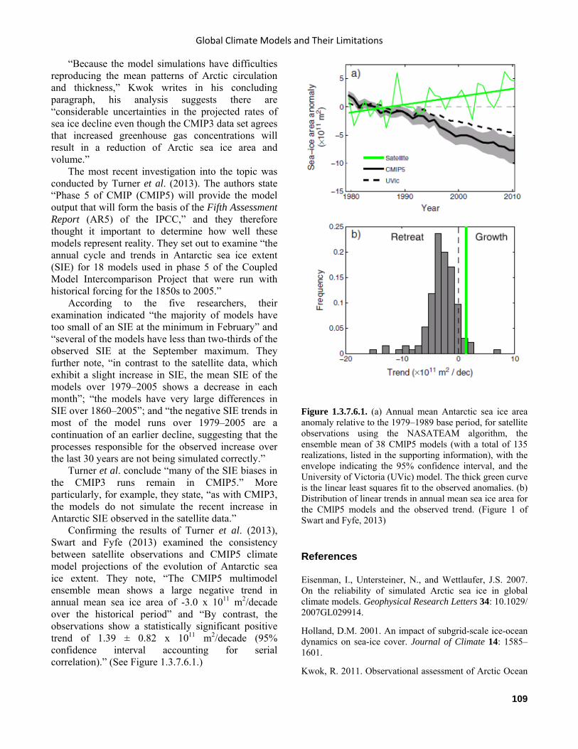
Global Climate Models and Their Limitations
109
“Because the model simulations have difficulties reproducing the mean patterns of Arctic circulation and thickness,” Kwok writes in his concluding paragraph, his analysis suggests there are “considerable uncertainties in the projected rates of sea ice decline even though the CMIP3 data set agrees that increased greenhouse gas concentrations will result in a reduction of Arctic sea ice area and volume.”
The most recent investigation into the topic was conducted by Turner et al. (2013). The authors state “Phase 5 of CMIP (CMIP5) will provide the model output that will form the basis of the Fifth Assessment Report (AR5) of the IPCC,” and they therefore thought it important to determine how well these models represent reality. They set out to examine “the annual cycle and trends in Antarctic sea ice extent (SIE) for 18 models used in phase 5 of the Coupled Model Intercomparison Project that were run with historical forcing for the 1850s to 2005.”
According to the five researchers, their examination indicated “the majority of models have too small of an SIE at the minimum in February” and “several of the models have less than two-thirds of the observed SIE at the September maximum. They further note, “in contrast to the satellite data, which exhibit a slight increase in SIE, the mean SIE of the models over 1979–2005 shows a decrease in each month”; “the models have very large differences in SIE over 1860–2005”; and “the negative SIE trends in most of the model runs over 1979–2005 are a continuation of an earlier decline, suggesting that the processes responsible for the observed increase over the last 30 years are not being simulated correctly.”
Turner et al. conclude “many of the SIE biases in the CMIP3 runs remain in CMIP5.” More particularly, for example, they state, “as with CMIP3, the models do not simulate the recent increase in Antarctic SIE observed in the satellite data.”
Confirming the results of Turner et al. (2013), Swart and Fyfe (2013) examined the consistency between satellite observations and CMIP5 climate model projections of the evolution of Antarctic sea ice extent. They note, “The CMIP5 multimodel ensemble mean shows a large negative trend in annual mean sea ice area of -3.0 x 10¹¹ m2/decade over the historical period” and “By contrast, the observations show a statistically significant positive trend of 1.39 ± 0.82 x 10¹¹ m2/decade (95% confidence interval accounting for serial correlation).” (See Figure 1.3.7.6.1.)
References Eisenman, I., Untersteiner, N., and Wettlaufer, J.S. 2007. On the reliability of simulated Arctic sea ice in global climate models. Geophysical Research Letters 34: 10.1029/ 2007GL029914.
Holland, D.M. 2001. An impact of subgrid-scale ice-ocean dynamics on sea-ice cover. Journal of Climate 14: 1585–1601.
Kwok, R. 2011. Observational assessment of Arctic Ocean
Figure 1.3.7.6.1. (a) Annual mean Antarctic sea ice area anomaly relative to the 1979–1989 base period, for satellite observations using the NASATEAM algorithm, the ensemble mean of 38 CMlP5 models (with a total of 135 realizations, listed in the supporting information), with the envelope indicating the 95% confidence interval, and the University of Victoria (UVic) model. The thick green curve is the linear least squares fit to the observed anomalies. (b) Distribution of linear trends in annual mean sea ice area for the CMlP5 models and the observed trend. (Figure 1 of Swart and Fyfe, 2013)
Climate Change Reconsidered II
110
sea ice motion, export, and thickness in CMIP3 climate simulations. Journal of Geophysical Research 116: 10.1029/2011JC007004.
Laxon, S., Peacock, N., and Smith, D. 2003. High interannual variability of sea ice thickness in the Arctic region. Nature 425: 947–950.
Meehl, G.A., Covey, C., Delworth, T., Latif, M., McAvaney, B., Mitchell, J.F.B., Stouffer, R.J., and Taylor, K.E. 2007. The WCRP CMIP3 multi-model dataset: A new era in climate change research. Bulletin of the American Meteorological Society 88: 1383–1394.
Stroeve, J., Holland, M.M., Meier, W., Scambos, T., and Serreze, M. 2007. Arctic sea ice decline: Faster than forecast. Geophysical Research Letters 34: 10.1029/ 2007GL029703.
Swart, N.C. and Fyfe, J.C., 2013. The influence of recent Antarctic ice sheet retreat on simulated sea iec area trends. Geophysical Research Letters 40: 10.1002/grl.50820.
Turner, J., Bracegirdle, T.J., Phillips, T., Marshall, G.J., and Hosking, J.S. 2013. An initial assessment of Antarctic sea ice extent in the CMIP5 models. Journal of Climate 26: 1473–1484. doi: http://dx.doi.org/10.1175/JCLI-D-12-00068.1
Zhang, X. and Walsh, J.E. 206. Toward a seasonally ice-covered Arctic Ocean: Scenarios from the IPCC AR4 model simulations. Journal of Climate 19: 1730–1747.
1.3.8 Soil Moisture Climate models have long indicated that CO2-induced global warming will increase evapotranspiration, causing decreases in soil moisture content that may offset modest increases in continental precipitation and lead to greater aridity in both water-limited natural ecosystems and lands devoted to agriculture (Manabe and Wetherald, 1986; Rind, 1988; Gleick, 1989; Vlades et al., 1994; Gregory et al., 1997; Komescu et al., 1998). This section examines pertinent scientific literature to assess this claim.
In a turn-of-the century evaluation of how climate modelers had progressed in their efforts to improve their simulations of soil moisture content over the prior few years, Srinivasan et al. (2000) examined “the impacts of model revisions, particularly the land surface representations, on soil moisture simulations, by comparing the simulations to actual soil moisture observations.” They write, “the revised models do not show any systematic improvement in their ability to simulate observed seasonal variations of soil moisture over the regions studied.” They also note, “there are no indications of conceptually more realistic land
surface representations producing better soil moisture simulations in the revised climate models.” They report a “tendency toward unrealistic summer drying in several models,” which they note was “particularly relevant in view of the summer desiccation projected by GCMs considered in future assessments of climate change.”
Although Srinivasan et al. report “simpler land-surface parameterization schemes are being replaced by conceptually realistic treatments,” as the climate modeling enterprise evolves, they note “improvements gained by such changes are ... not very apparent.”
A similar assessment was supplied that year by Robock et al. (2000), who developed a massive collection of soil moisture data for more than 600 stations from a wide variety of climatic regimes found within the former Soviet Union, China, Mongolia, India, and the United States. In describing these data sets they also state an important ground rule. Sometimes, they note, “the word ‘data’ is used to describe output from theoretical model calculations, or values derived from theoretical analysis of radiances from remote sensing.” However, they state, “we prefer to reserve this word for actual physical observations,” noting “all the data in our data bank are actual in situ observations.”
This distinction is important, for one of the illuminating analyses Robock et al. performed with their data was to check summer soil moisture trends simulated by the Geophysical Fluid Dynamics Laboratory’s general circulation model of the atmosphere as forced by transient CO2 and tropospheric sulfate aerosols for specific periods and regions for which they had actual soil moisture data. They found, “although this model predicts summer desiccation in the next century, it does not in general reproduce the observed upward trends in soil moisture very well,” a mammoth understatement considering the predictions and observations go in opposite directions. As noted elsewhere in their paper, “in contrast to predictions of summer desiccation with increasing temperatures, for the stations with the longest records, summer soil moisture in the top 1 m has increased while temperatures have risen.”
Another important report on the subject is presented five years later, again by Robock et al. (2005), who note “most global climate model simulations of the future, when forced with increasing greenhouse gases and anthropogenic aerosols, predict summer desiccation in the midlatitudes of the Northern Hemisphere (e.g., Gregory et al., 1997;

Global Climate Models and Their Limitations
111
Wetherald and Manabe, 1999; Cubasch et al., 2001),” adding “this predicted soil moisture reduction, the product of increased evaporative demand with higher temperatures overwhelming any increased precipitation, is one of the gravest threats of global warming, potentially having large impacts on our food supply.”
With the explicit intent “to evaluate these model simulations,” the three American and two Ukrainian scientists present “the longest data set of observed soil moisture available in the world, 45 years of gravimetrically-observed plant available soil moisture for the top 1 m of soil, observed every 10 days for April-October for 141 stations from fields with either winter or spring cereals from the Ukraine for 1958-2002.” As they describe it, “the observations show a positive soil moisture trend for the entire period of observation, with the trend leveling off in the last two decades,” noting “even though for the entire period there is a small upward trend in temperature and a downward trend in summer precipitation, the soil moisture still has an upward trend for both winter and summer cereals.”
In light of these real-world observations, Robock et al. note “although models of global warming predict summer desiccation in a greenhouse-warmed world, there is no evidence for this in the observations yet, even though the region has been warming for the entire period.” In attempting to explain this dichotomy, they state the real-world increase in soil moisture content may have been driven by a downward trend in evaporation caused by the controversial “global dimming” hypothesis (Liepert et al., 2004). Alternatively, we offer it may have been driven by the well-known anti-transpirant effect of atmospheric CO2 enrichment, which tends to conserve water in the soils beneath crops and thereby leads to enhanced soil moisture contents, as has been demonstrated in a host of experiments conducted in real-world field situations.
One especially outstanding study in this regard is that of Zaveleta et al. (2003), who tested the hypothesis that soil moisture contents may decline in a CO2-enriched and warmer world, in a two-year study of an annual-dominated California grassland at the Jasper Ridge Biological Preserve, Stanford, California, USA, where they delivered extra heating to a number of free-air CO2 enrichment (FACE) plots (enriched with an extra 300 ppm of CO2) via IR heat lamps suspended over the plots that warmed the surface of the soil beneath them by 0.8-1.0°C.
The individual effects of atmospheric CO2
enrichment and soil warming were of similar magnitude, and acting together they enhanced mean spring soil moisture content by about 15 percent over that of the control treatment. The effect of CO2 was produced primarily as a consequence of its ability to cause partial stomatal closure and thereby reduce season-long plant water loss via transpiration. In the case of warming, there was an acceleration of canopy senescence that further increased soil moisture by reducing the period of time over which transpiration losses occur, all without any decrease in total plant production.
Zaveleta et al. note their findings “illustrate the potential for organism-environment interactions to modify the direction as well as the magnitude of global change effects on ecosystem functioning.” Whereas model projections suggest vast reaches of agricultural land will dry up and be lost to profitable production in a CO2-enriched world of the future, this study suggests just the opposite could occur. As the six researchers describe it, “we suggest that in at least some ecosystems, declines in plant transpiration mediated by changes in phenology can offset direct increases in evaporative water losses under future warming.”
Guo and Dirmeyer (2006) compared soil moisture simulations made by 11 models in the Second Global Soil Wetness Project, a multi-institutional modeling research activity intended to produce a complete multi-model set of land surface state variables and fluxes by using land surface models driven by the 10-year period of data provided by the International Satellite Land Surface Climatology Project Initiative II, against real-world observations made on the top meter of grassland and agricultural soils located within parts of the former Soviet Union, the United States (Illinois), China, and Mongolia that are archived in the Global Soil Moisture Data Bank.
According to the authors, “simulating the actual values of observed soil moisture is still a challenging task for all models,” as they note “both the root mean square of errors (RMSE) and the spread of RMSE across models are large” and “the absolute values of soil moisture are poorly simulated by most models.” In addition, they report “within regions there can be tremendous variations of any model to simulate the time series of soil moisture at different stations.”
Guo and Dirmeyer suggest the errors and variations are serious problems for the models. First, the two researchers write “the land surface plays a vital role in the global climate system through interactions with the atmosphere.”They also note
Climate Change Reconsidered II
112
“accurate simulation of land surface states is critical to the skill of weather and climate forecasts” and soil moisture “is the definitive land surface state variable; key for model initial conditions from which the global weather and climate forecasts begin integrations, and a vital factor affecting surface heat fluxes and land surface temperature.”
In their own study of the subject, Li et al. (2007) compared soil moisture simulations derived from the IPCC’s AR4 climate models, which were driven by observed climate forcings, for the period 1958–1999 with actual measurements of soil moisture made at more than 140 stations or districts in the mid-latitudes of the Northern Hemisphere. The latter were averaged in such a way as to yield six regional results: one each for the Ukraine, Russia, Mongolia, Northern China, Central China, and Illinois (USA). According to the three researchers, the models showed realistic seasonal cycles for the Ukraine, Russia, and Illinois but “generally poor seasonal cycles for Mongolia and China.” In addition, they report the Ukraine and Russia experienced soil moisture increases in summer “that were larger than most trends in the model simulations.” The researchers found “only two out of 25 model realizations show trends comparable to those observations,” and the two realistic model-derived trends were “due to internal model variability rather than a result of external forcing,” which means the two reasonable matches were in fact accidental.
Noting further “changes in precipitation and temperature cannot fully explain soil moisture increases for [the] Ukraine and Russia,” Li et al. write, “other factors might have played a dominant role on the observed patterns for soil moisture.” They mention solar dimming, plus the fact that in response to elevated atmospheric CO2 concentrations, “many plant species reduce their stomatal openings, leading to a reduction in evaporation to the atmosphere,” so “more water is likely to be stored in the soil or [diverted to] runoff,” reporting this phenomenon was detected in continental river runoff data by Gedney et al. (2006).
Publishing in Geophysical Research Letters, Christensen and Boberg (2012) describe how they compared monthly mean temperatures projected by 34 global climate models included in phase 5 of the Coupled Model Intercomparison Project (CMIP5) with observations from the University of East Anglia’s Climatic Research Unit for 26 different regions covering all major land areas of the world for the period 1961–2000, for which they employed quantile-quantile (q-q) diagrams. This revealed the
existence of “a warm period positive temperature dependent bias” for “many of the models with many of the chosen climate regions”; the magnitude of this temperature dependence varied considerably among the models.
Analyzing the role of this difference as “a contributing factor for some models to project stronger regional warming than others,” the two scientists found “models with a positive temperature dependent bias tend to have a large projected temperature change” and “these tendencies increase with increasing global warming level.” In addition, they state this situation “appears to be linked with the ability of models to capture complex feedbacks accurately,” noting in particular that land-surface/atmosphere interactions are treated differently and with different degrees of realism among the various models they investigated and “soil moisture-temperature feedbacks are relevant for temperature extremes in a large fraction of the globe.”
Christensen and Boberg conclude, “accepting model spread as a way to portray uncertainty of the projection estimate may result in an overestimation of the projected warming and at the same time indicate little model agreement on the mean value.” They note “a non-negligible part” of this overestimation “is due to model deficiencies” that have yet to be overcome.
In light of the observations discussed above, it would appear almost all climate models employed to date have greatly erred with respect to what Robock et al. (2005) describe as “one of the gravest threats of global warming”—soil moisture content. Not only has the model-predicted decline in Northern Hemispheric midlatitude soil moisture contents failed to materialize under the combined influence of many decades of rising atmospheric CO2 concentrations and temperatures, it has become less of a threat, possibly as a consequence of biological impacts of the ongoing rise in the air’s CO2 content. References Christensen, J.H. and Boberg, F. 2012. Temperature dependent climate projection deficiencies in CMIP5 models. Geophysical Research Letters 39: 10.1029/ 2012GL053650.
Cubasch, U., Meehl, G.A., Boer, G.J., Stouffer, R.J., Dix, M., Noda, A., Senior, C.A., Raper, S., and Yap, K.S. 2001. Projections of future climate change. In: Houghton, J.T. et al. (Eds.) Climate Change 2001: The Scientific Basis: Contribution of Working Group I to the Third Assessment Report of the Intergovernmental Panel on Climate Change,
Global Climate Models and Their Limitations
113
Cambridge University Press, Cambridge, New York, USA, pp. 525–582.
Gedney, N., Cox, P.M., Betts, R.A., Boucher, O., Huntingford, C., and Stott, P.A. 2006. Detection of a direct carbon dioxide effect in continental river runoff records. Nature 439: 835–838.
Gleick, P.H. 1989. Climate change, hydrology and water resources. Reviews of Geophysics 27: 329–344.
Gregory, J.M., Mitchell, J.F.B., and Brady, A.J. 1997. Summer drought in northern midlatitudes in a time-dependent CO2 climate experiment. Journal of Climate 10: 662–686.
Guo, Z. and Dirmeyer, P.A. 2006. Evaluation of the Second Global Soil Wetness Project soil moisture simulations: 1. Intermodel comparison. Journal of Geophysical Research 111: 10.1029/2006JD007233.
Komescu, A.U., Eikan, A., and Oz, S. 1998. Possible impacts of climate change on soil moisture availability in the Southeast Anatolia Development Project Region (GAP): An analysis from an agricultural drought perspective. Climatic Change 40: 519–545.
Li, H., Robock, A., and Wild, M. 2007. Evaluation of Intergovernmental Panel on Climate Change Fourth Assessment soil moisture simulations for the second half of the twentieth century. Journal of Geophysical Research 112: 10.1029/2006JD007455.
Liepert, B.G., Feichter, J., Lohmann, U., and Roeckner, E. 2004. Can aerosols spin down the water cycle in a warmer and moister world? Geophysical Research Letters 31: 10.1029/2003GL019060.
Manabe, S. and Wetherald, R.T. 1986. Reduction in summer soil wetness induced by an increase in atmospheric carbon dioxide. Science 232: 626–628.
Rind, D. 1988. The doubled CO2 climate and the sensitivity of the modeled hydrologic cycle. Journal of Geophysical Research 93: 5385–5412.
Robock, A., Mu, M., Vinnikov, K., Trofimova, I.V., and Adamenko, T.I. 2005. Forty-five years of observed soil moisture in the Ukraine: No summer desiccation (yet). Geophysical Research Letters 32: 10.1029/2004GL021914.
Robock, A., Vinnikov, K.Y., Srinivasan, G., Entin, J.K., Hollinger, S.E., Speranskaya, N.A., Liu, S., and Namkhai, A. 2000. The global soil moisture data bank. Bulletin of the American Meteorological Society 81: 1281–1299.
Srinivasan, G., Robock, A., Entin, J.K., Luo, L., Vinnikov, K.Y., Viterbo, P., and Participating AMIP Modeling Groups. 2000. Soil moisture simulations in revised AMIP models. Journal of Geophysical Research 105: 26,635–26,644.
Vlades, J.B., Seoane, R.S., and North, G.R. 1994. A methodology for the evaluation of global warming impact on soil moisture and runoff. Journal of Hydrology 161: 389–413.
Wetherald, R.T. and Manabe, S. 1999. Detectability of summer dryness caused by greenhouse warming. Climatic Change 43: 495–511.
Zavaleta, E.S., Thomas, B.D., Chiariello, N.R., Asner, G.P., Shaw, M.R., and Field, C.B. 2003. Plants reverse warming effect on ecosystem water balance. Proceedings of the National Academy of Science USA 100: 9892–9893.
1.3.9 Biological Processes In a landmark paper published in Global Change Biology, Eastman et al. (2001) described the first comprehensive study of CO2-induced regional climate change based on a hybrid atmosphere/vegetation model composed of linked meteorological and plant growth sub-models.
The authors of the groundbreaking study began by citing a number of peer-reviewed scientific research papers that demonstrated the likelihood of what they called “a crucial role for biospheric feedbacks on climate,” including processes driven by CO2-induced changes in land surface albedo, leaf stomatal conductance, plant rooting profile, fractional coverage of the land by vegetation, plant roughness length and displacement height, vegetation phenology, time of planting and harvesting (in the case of agricultural crops), and plant growth. Next, they validated the model against real-world meteorological and plant growth data obtained for the 1989 growing season for the area located between approximately 35° and 48° N latitude and 96° and 110° W longitude. Last, they investigated how the climate of the region changes when (1) only the radiative effects of a doubling of the air’s CO2 concentration are considered, (2) only the biological effects of a doubling of the air’s CO2 concentration are considered, and (3) the radiative and biological effects of a doubling of the air’s CO2 concentration occur simultaneously.
With respect to the area-averaged and seasonally averaged daily maximum air temperature, the radiative effects of a doubling of the atmospheric CO2 concentration lead to a warming of only 0.014°C, and the biological effects of the extra CO2 produced a cooling of fully 0.747°C. Considered together and including a nonlinear interaction term, the simultaneous radiative and biological effects of a doubling of the air’s CO2 content thus produced a net
Climate Change Reconsidered II
114
cooling of 0.715°C. With respect to the area-averaged and seasonally
averaged daily minimum air temperature, the radiative effects of a doubling of the atmospheric CO2 concentration led to a warming of 0.097°C, while the biological effects of the extra CO2 produced a warming of 0.261°C. Considered together and again including the nonlinear interaction term, the simultaneous radiative and biological effects of a doubling of the air’s CO2 content thus produced a net warming of 0.354°C.
During the day, then, when high air temperatures can be detrimental to both plant and animal life, the combined effect of the simultaneous radiative and biological impacts of an increase in the air’s CO2 content acts to decrease daily maximum air temperature, alleviating potential heat stress. During the night, when low temperatures can be detrimental to plant and animal life, the combined effect of the radiative and biological impacts of an increase in the air’s CO2 content acts to increase daily minimum air temperature, alleviating potential cold stress. When considering the day and night air temperature changes together, the mean daily air temperature range is reduced by approximately 1.069°C, leading to a more thermally stable environment, which in this case was also about 0.180°C cooler in the mean.
The authors also found the CO2-induced change in area-averaged and seasonally averaged leaf area index was increased (+21.8%) with the simultaneous expression of the radiative and biological effects of a doubling of the air’s CO2 content.
In summarizing their findings, the authors report “it is clear” the radiative effects of a doubling of the air’s CO2 content have “little effect on anything” and play but a “minor role in the coupled biological and atmospheric system.” The authors acknowledge their analysis is “a regional-scale sensitivity study,” the results of which “cannot be linearly scaled up to global scales.”
Nevertheless the authors follow that caveat by noting their results “suggest that the regional response could be on the order of global climate sensitivities.” Thus they conclude, “climate change that results from anthropogenic increases of CO2 must consider the biological effects of enriched CO2 as well as its radiative effect.” Most models exclude this important interaction.
In a paper published a decade later, Delire et al. (2011) used the CCMv3 and LMDz atmospheric GCMs and coupled these models to the latest versions of the Integrated Biosphere Simulator (IBIS) (Foley et
al. 1996) and the ORCHIDEE biosphere model (Krinner et al. 2005), respectively. Each is a land surface model that includes plant characteristics such as the physiology of plant cover, plant phenology, carbon cycling, plant type competition, photosynthesis, and respiration. Both include daily and annual vegetation cycles and distinguish between trees and other types of vegetation (grasses, shrubs). Delire et al. ran each model with full capabilities and then by keeping the vegetation constant (fixed).
The GCM modeling strategy used by Delire et al. was to simulate the climate using observed sea surface temperatures from 1870–1899 available from the Hadley Centre in England. Their goal was to remove the impact of the ocean in order to highlight land-surface process differences in the coupled systems. The model was run for 400 years; the last 300 were used for analysis.
The interannual variability in plant cover generated by both models was similar to that of observed plant cover variability derived using satellite observations for 1982–1994. The LMDz-ORCHIDEE model showed stronger interannual variability, but in both the variability in tree cover was less than 5 percent, whereas for grasses it could be as much as 10 to 20 percent. Vegetation affected climate, as inferred by comparing the dynamic to fixed vegetation. The model strategy precluded comparison with observed climate.
The dynamic vegetation runs showed stronger low frequency variability than the fixed runs for both temperature and precipitation for each model system, but the disparity between the fixed and dynamic run was stronger for the CCMv3-IBIS system (Figure 1.3.9.1). The strength of the variability (0.05-2.0°C) compared favorably to that inferred by previous studies. The feedback between temperature and plant growth was generally positive (warmer temperatures, increased vegetation) in the mid-latitudes and poleward. The feedback was generally negative and weaker in semi-arid regions (increased vegetation, more evaporation, cooler temperatures). There was only a weak positive feedback in the precipitation over most areas of the globe.
As we begin to understand more about the climate system, including the complexity of heat and mass exchange between various portions of it, we can more effectively model the past climate, including its variability. However, many of the climate simulations used to project future climate are fairly simple models that do not include a dynamic ocean or realistic representations of biological processes on land. These
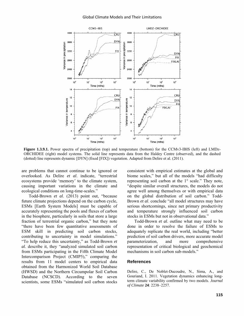
Global Climate Models and Their Limitations
115
are problems that cannot continue to be ignored or overlooked. As Delire et al. indicate, “terrestrial ecosystems provide ‘memory’ to the climate system, causing important variations in the climate and ecological conditions on long-time-scales.”
Todd-Brown et al. (2013) point out, “because future climate projections depend on the carbon cycle, ESMs [Earth System Models] must be capable of accurately representing the pools and fluxes of carbon in the biosphere, particularly in soils that store a large fraction of terrestrial organic carbon,” but they note “there have been few quantitative assessments of ESM skill in predicting soil carbon stocks, contributing to uncertainty in model simulations.” “To help reduce this uncertainty,” as Todd-Brown et al. describe it, they “analyzed simulated soil carbon from ESMs participating in the Fifth Climate Model Intercomparison Project (CMIP5),” comparing the results from 11 model centers to empirical data obtained from the Harmonized World Soil Database (HWSD) and the Northern Circumpolar Soil Carbon Database (NCSCD). According to the seven scientists, some ESMs “simulated soil carbon stocks
consistent with empirical estimates at the global and biome scales,” but all of the models “had difficulty representing soil carbon at the 1° scale.” They note, “despite similar overall structures, the models do not agree well among themselves or with empirical data on the global distribution of soil carbon.” Todd-Brown et al. conclude “all model structures may have serious shortcomings, since net primary productivity and temperature strongly influenced soil carbon stocks in ESMs but not in observational data.”
Todd-Brown et al. outline what may need to be done in order to resolve the failure of ESMs to adequately replicate the real world, including “better prediction of soil carbon drivers, more accurate model parameterization, and more comprehensive representation of critical biological and geochemical mechanisms in soil carbon sub-models.” References Delire, C., De Noblet-Ducoudre, N., Sima, A., and Gouriand, I. 2011. Vegetation dynamics enhancing long-term climate variability confirmed by two models. Journal of Climate 24: 2238–2257.
Figure 1.3.9.1. Power spectra of precipitation (top) and temperature (bottom) for the CCMv3-IBIS (left) and LMDz-ORCHIDEE (right) model systems. The solid line represents data from the Haldey Centre (observed), and the dashed (dotted) line represents dynamic [DYN] (fixed [FIX]) vegetation. Adapted from Delire et al. (2011).

Climate Change Reconsidered II
116
Eastman, J.L., Coughenour, M.B., and Pielke Sr., R.A. 2001. The regional effects of CO2 and landscape change using a coupled plant and meteorological model. Global Change Biology 7: 797–815.
Foley, J.A., Prentice, C.I., Ramankutty, N., Levis, S., Pollard, D., Sitch, S., and Haxeltine, A. 1996. An integrated biosphere model of land surface processes, terrestrial carbon balance, and vegetation dynamics. Global Biogeochemical Cycles 10: 603–628.
Krinner, G., Viovy, N., de Noblet-Ducoudré, N., Ogée, J., Polcher, J., Friedlingstein, P., Ciais, P., Sitch, S., and Prentice, I.C. 2005. A dynamic global vegetation model for studies of the coupled atmosphere-biosphere system. Global Biogeochemical Cycles 19: 1–33.
Todd-Brown, K.E.O., Randerson, J.T., Post, W.M., Hoffman, F.M., Tarnocai, C., Schuur, E.A.G., and Allison, S.D. 2013. Causes of variation in soil carbon simulations from CMIP5 Earth system models and comparison with observations. Biogeosciences 10: 1717–1736.
1.3.10 Permafrost Almost all assessments of the potential impacts of climate change on the world’s permafrost are based on a two-layer model that incorporates a seasonally frozen active layer and an underlying perennially frozen soil. Shur et al. (2005) examined the virtues of adding a transition zone layer to produce a more realistic three-layer model.
Through a review of the literature and theoretical and data analyses, Shur et al. showed, among other things, that the transition zone alternates between seasonally frozen ground and permafrost over sub-decadal to centennial time scales, functioning as a buffer between the active layer and the underlying perennial permafrost by increasing the latent heat required for thaw. Consequently, in the words of Shur et al., use of a two-layer conceptual model in permafrost studies “obscures effective understanding of the formation and properties of the upper permafrost and syngenetic permafrost, and makes a realistic determination of the stability of arctic geosystems under climatic fluctuations virtually impossible.” They conclude “the impacts of possible global warming in permafrost regions cannot be understood fully without consideration of a more realistic three-layer model.”
In light of the authors’ findings, it would appear two-layer model forecasts of future permafrost trends under various global warming scenarios are inadequate. And if the transition zone does indeed act as a buffer at sub-decadal to centennial time scales,
then current permafrost trends are likely to be manifestations of past climatic trends, some of which may have taken place several decades ago or more.
Koven et al. (2013) note “permafrost is a critical component of high-latitude land and determines the character of the hydrology, ecology, and biogeochemistry of the region.” Therefore, they write, there is “widespread interest in the use of coupled atmosphere-ocean-land surface models to predict the fate of permafrost over the next centuries because (1) permafrost contains the largest organic carbon (C) reservoir in the terrestrial system (Tarnocai et al., 2009), (2) permafrost stability is primarily dependent on temperature, and (3) global warming is expected to be relatively larger over the permafrost domain because of arctic amplification processes (Holland and Bitz, 2003).”
Koven et al. analyzed “output from a set of Earth system models (ESMs) that participated in phase 5 of the Coupled Model Intercomparison Project (CMIP5) (Taylor et al., 2009) to evaluate the permafrost model predictions against observations and theoretical expectations and to compare the predicted fate of permafrost under warming scenarios.” The three U.S. researchers revealed “the models show a wide range of behaviors under the current climate, with many failing to agree with fundamental aspects of the observed soil thermal regime at high latitudes.”
Koven et al. report, “under future climate change, the models differ in their degree of warming, both globally and at high latitudes, and also in the response of permafrost to this warming.” They note “there is a wide range of possible magnitudes in their responses, from 6% to 29% permafrost loss per 1°C high-latitude warming.” Several of the models, they report, “predict substantial permafrost degradation has already occurred (ranging from 3% gain to 49% loss relative to 1850 conditions)” and “the majority of models at the high end of relative twentieth-century permafrost loss also show unrealistically small preindustrial permafrost extent.” They also note “there is wide model disagreement on the value of the difference in mean temperature across the air-soil interface, with several of the models [even] predicting the wrong sign for this statistic” and “there is wide model disagreement in the changes of [the] mean and [the] amplitude of soil temperatures with depth.”
Koven et al. conclude by stating, “with this analysis, we show that widespread disagreement exists among this generation of ESMs,” once again suggesting current Earth system models are not yet accurate enough for real-world application.

Global Climate Models and Their Limitations
117
References Holland, M.M. and Bitz, C.M. 2003. Polar amplification of climate change in coupled models. Climate Dynamics 21: 221–232.
Koven, C.D., Riley, W.J., and Stern, A. 2013. Analysis of permafrost thermal dynamics and response to climate change in the CMIP5 earth system models. Journal of Climate 26: 1877–1900.
Shur, Y., Hinkel, K.M., and Nelson, F.E. 2005. The transient layer: implications for geocryology and climate-change science. Permafrost and Periglacial Processes 16: 5–17.
Tarnocai, C., Canadell, J.G., Schuur, E.A.G., Kuhry, P., Mazhitova, G., and Zimov, S. 2009. Soil organic carbon pools in the northern circumpolar permafrost region. Global Biogeochemical Cycles 23: 10.1029/ 2008GB003327.
Taylor, K.E., Stouffer, R.J., and Meehl, G.A. 2009. A Summary of the CMIP5 Experiment Design. Technical Report: Program for Climate Model Diagnosis and Intercomparison. Lawrence Livermore National Laboratory, Livermore, California, USA.
1.3.11 Miscellaneous Several other studies have documented inadequacies in climate model projections. This subsection highlights those that do not quite fit in other subsections of Section 1.4 or that deal with multiple climatic elements and, as such, are best suited for this miscellaneous category.
“Climate variability,” in the words of Latif and Keenlyside (2011), “can be either generated internally by interactions within or between the individual climate subcomponents (e.g., atmosphere, ocean and sea ice) or externally by e.g., volcanic eruptions, variations in the solar insolation at the top of the atmosphere, or changed atmospheric greenhouse gas concentrations in response to anthropogenic emissions.” Some examples of these internal variations are “the North Atlantic Oscillation (NAO), the El Niño/Southern Oscillation (ENSO), the Pacific Decadal Variability (PDV), and the Atlantic Multidecadal Variability (AMV),” all of which “project on global or hemispheric surface air temperature (SAT), thereby masking anthropogenic climate change.”
In a review of this complex subject, Latif and Keenlyside—who hold positions at Germany’s Leibniz-Institute for Meerewissenschaften at the
University of Kiel—first describe various mechanisms responsible for internal variability, giving special attention to the variability of the Atlantic Meridional Overturning Circulation (AMOC), which they suggest is likely the origin of a considerable part of the decadal variability within the Atlantic Sector, after which they discuss the challenge of decadal SAT predictability and various factors limiting its realization.
The two researchers identify numerous problems that hamper decadal climate predictability, including that “the models suffer from large biases.” In the cases of annual mean sea surface temperature (SST) and SAT over land, for example, they state “typical errors can amount up to 10°C in certain regions,” as Randall et al. (2007) found to be the case for many of the IPCC-AR4 models. Latif and Keenlyside also note several models “fail to simulate a realistic El Niño/Southern Oscillation.” In addition, the researchers point out “several assumptions have generally to be made about the process under consideration that cannot be rigorously justified, and this is a major source of uncertainty.”
Another problem they discuss is that “some components of the climate system are not well represented or not at all part of standard climate models,” one example being the models’ neglect of the stratosphere. This omission is serious; Latif and Keenlyside say “recent studies indicate that the mid-latitudinal response to both tropical and extra-tropical SST anomalies over the North Atlantic Sector may critically depend on stratospheric feedbacks,” noting Ineson and Scaife (2009) present evidence for “an active stratospheric role in the transition to cold conditions in northern Europe and mild conditions in southern Europe in late winter during El Niño years.”
An additional common model shortcoming, even in standalone integrations with models forced by observed SSTs, is that model simulations of rainfall in the Sahel “fail to reproduce the correct magnitude of the decadal precipitation anomalies.” Still another failure, as shown by Stroeve et al. (2007), is that “virtually all climate models considerably underestimate the observed Arctic sea ice decline during the recent decades in the so-called 20th century integrations with prescribed (known natural and anthropogenic) observed forcing.” In addition, “atmospheric chemistry and aerosol processes are still not well incorporated into current climate models.”
In summing up their findings, which include those noted above and many more, Latif and Keenlyside state, “a sufficient understanding of the
Climate Change Reconsidered II
118
mechanisms of decadal-to-multidecadal variability is lacking.” They note “state-of-the-art climate models suffer from large biases” and “are incomplete and do not incorporate potentially important physics.” Various mechanisms “differ strongly from model to model,” they point out; “the poor observational database does not allow a distinction between ‘realistic’ and ‘unrealistic’ simulations”; and many models “still fail to simulate a realistic El Niño/Southern Oscillation.” Therefore, they conclude, “it cannot be assumed that current climate models are well suited to realize the full decadal predictability potential”—a somewhat obscure way of stating current state-of-the-art climate models are not good enough to make reasonably accurate simulations of climate change over a period of time (either in the past or the future) that is measured in mere decades.
In another paper, Lucarini et al. (2007) compared for the period 1962–2000 “the estimate of the northern hemisphere mid-latitude winter atmospheric variability within the available 20th century simulations of 19 global climate models included in the Intergovernmental Panel on Climate Change [IPCC] 4th Assessment Report” with “the NCEP-NCAR and ECMWF reanalyses,” compilations of real-world observations produced by the National Center for Environmental Prediction (NCEP), in collaboration with the National Center for Atmospheric Research (NCAR), and by the European Center for Mid-Range Weather Forecast (ECMWF). The five Italian researchers report “large biases, in several cases larger than 20%, are found in all the considered metrics between the wave climatologies of most IPCC models and the reanalyses, while the span of the climatologies of the various models is, in all cases, around 50%.” They also report “the traveling baroclinic waves are typically overestimated by the climate models, while the planetary waves are usually underestimated,” and “the model results do not cluster around their ensemble mean.” The authors conclude by stating, “this study suggests caveats with respect to the ability of most of the presently available climate models in representing the statistical properties of the global scale atmospheric dynamics of the present climate and, a fortiori [“all the more,” as per Webster’s Dictionary], in the perspective of modeling climate change.”
According to Scherrer (2011), “climate model verification primarily focused [in the past] on the representation of climatological means.” But “on the other hand,” he continues, “a good representation of second-order moments (i.e., variability) on different
time scales (e.g., daily, month-to-month, or interannual, etc.) is crucial and probably provides an even better test as to whether [real-world] physical processes are well represented in the models.” Working with twentieth century climate model runs prepared within the context of the IPCC AR4 assessment (now called the CMIP3 data set), Scherrer set out to compare model simulations of the interannual variability (IAV) of 2-m-height air temperature (T), sea level pressure (SLP), and precipitation (P) over the twentieth century with observational and reanalysis data sets for the same time period using standard deviation-based variability indices.
The Swiss scientist describes a number of problems he encountered with the CMIP3 models. With respect to SLP, the situation was pretty good: “only minor IAV problems are found.” With respect to temperature, however, differences between observations and models are, in general, “larger than those for SLP.” And for precipitation, “IAV is ‘all over the place’ and no clear relations with T and SLP IAV problems can be established.”
Concentrating thereafter mostly on temperature, Scherrer notes “a few models represent T IAV much worse than others and create spurious relations of IAV representation and the climate change signal.” Among the “better” IAV models, he finds “the ‘good’ IAV models in the tropics are in general not also the ‘good’ IAV models in the extra-tropics,” and “the ‘good’ IAV models over the sea are in general not the ‘good’ IAV models over land.” He further notes “similar results are found for the relation between T IAV representation and the amplitude of projected changes in temperature.”
“In general,” Scherrer writes, “it is concluded that, aggregated over very large regions, hardly any robust relations exist between the models’ ability to correctly represent IAV and the projected temperature change.” He says these results represent “a plea to remove the ‘obviously wrong’ models (e.g., like those that have sea ice extending to below 50°N in the Atlantic and DJF temperature biases of ~40°C in Iceland, cf. Raisanen, 2007) before doing climate analyses.”
de Boer et al. (2012) point out “observed and projected changes in the Arctic region are some of the most striking concerns surrounding climate trends,” noting the latter “likely have important consequences both within the Arctic and globally.” They further note “a new generation of Earth system models has been utilized to prepare climate projections for the
Global Climate Models and Their Limitations
119
fifth phase of the Coupled Model Intercomparison Project (CMIP5),” the results of which are planned to be used “in the Intergovernmental Panel on Climate Change (IPCC) Fifth Assessment Report (AR5).” They set out to determine how well these models perform, but the closest they could come to conducting such a test was to interrogate the models used in the AR4 report of the IPCC. Thus, de Boer et al. simulated key features of the Arctic atmosphere in the Community Climate System Model, version 4 (CCSM4) and compared the results of those simulations “against observational and reanalysis datasets for the present-day (1981–2005).”
Describing problems they encountered in this endeavor, the seven scientists report “simulated surface air temperatures are found to be slightly too cold,” “evaluation of the sea level pressure [SLP] demonstrates some large biases, most noticeably an under simulation of the Beaufort High during spring and autumn,” “monthly Arctic-wide [SLP] biases of up to 13 mb are reported,” “cloud cover is under-predicted for all but summer months,” and “cloud phase is demonstrated to be different from observations.” They also found “simulated all-sky liquid water paths are too high,” “ice water path was generally too low,” and “precipitation is found to be excessive over much of the Arctic compared to ERA-40 and the Global Precipitation Climatology Project estimates.” They report “biases of 40%-150% are calculated over northern North America, northern Greenland, and the Arctic Ocean,” while “over the Norwegian Sea ... evaporation is over-simulated by up to 3.5 mm/day,” such that “P-E is generally too high over much of the Arctic, particularly over coastal Greenland.”
de Boer et al. also found “CCSM4 over-predicts surface energy fluxes during summer months” and “under-predicts it during winter.” They also report “the strengths of surface inversions were found to be too great in CCSM4 when compared to ERA-40, with distributions showing a near-doubling of strength,” and (15) “CCSM4 is found to have more inversions than ERA-40 for all months.”
Oddly, de Boer et al. conclude “CCSM4 provides a consistent representation of present-day Arctic climate” and “in doing so it represents individual components of the Arctic atmosphere with respectable accuracy.” This statement seems to us to be an egregious misuse of the word “respectable.”
Blazquez and Nuñez (2013) point out “the first step to understand climate changes that are likely to occur in the future is the assessment of the present
climate,” which “allows determining the model deficiencies.” The two authors set out to “[evaluate] a present climate simulation over southern South America performed with the Meteorological Research Institute/Japanese Meteorological Agency (MRI/ JMA) high resolution global model.”
Comparing their simulated wind results with data from the European Centre Medium Range Weather Forecasts (ECMWF) 40-year Reanalysis (ERA 40), and their temperature and precipitation simulations with data from various meteorological stations, the two Argentinian researchers report discovering significant model deficiencies: Speeds of the low level jet and the westerlies “are generally underestimated” and at upper levels “the westerlies are overestimated over central Argentina.” During December-February, March-May, and September-November, they report, “the MRI/JMA global model underestimates the temperature over east of Argentina, west of Uruguay, south of Chile and over tropical latitudes”and “overestimates are observed over central Argentina,” while “in June-August the model underestimates the temperature over most of Argentina, south of Chile and to the north of 20°S.” They also found “the model overestimates temperature interannual variability in all regions and all seasons, except in [June-July-August].”
With respect to precipitation, the authors found in all seasons the model yields “an underestimation of the precipitation in the southeast of Brazil and south of Peru and an overestimation in Bolivia, Uruguay, north and central Chile and north of Peru,” and during “the dry season (JJA) the model greatly overestimates the precipitation over northeastern and central Argentina.” They note “in regions located over mountainous areas the model presents a poor reproduction of the annual cycle” and “observed precipitation trends are generally positive whereas simulated ones are negative.”
Landrum et al. (2013) compared Last Millennium (LM) simulations of the Community Climate System Model, version 4 (CCSM4) to real-world “data reconstructions of temperature, the hydrologic cycle, and modes of climate variability.” In addition to some successes of the CCSM4, the seven scientists report a number of failures. They note “the LM simulation does not reproduce La Niña-like cooling in the eastern Pacific Ocean during the MCA [Medieval Climate Anomaly] relative to the LIA [Little Ice Age], as has been suggested by proxy reconstructions,” and “patterns of simulated precipitation change for the Asian monsoon to large
Climate Change Reconsidered II
120
volcanic eruptions have nearly opposite anomalies from those reconstructed from tree-ring chronologies.” They report CCSM4 “does not simulate a persistent positive NAO [North Atlantic Oscillation] or a prolonged period of negative PDO [Pacific Decadal Oscillation] during the MCA, as suggested by some proxy reconstructions” and “the model simulates cooling of ~1.0°-1.5°C after the large eruptions of the late thirteenth, mid-fifteenth, late eighteenth, and early nineteenth centuries, 2-3 times larger than the NH [Northern Hemisphere] summer anomalies estimated from tree-ring or multiproxy reconstructions.” They further report “twentieth-century simulations indicate that the CCSM4 hemispheric response to volcanic eruptions is stronger than observed (Meehl et al., 2012)” and they “do not find a persistent positive NAO or a prolonged period of negative PDO during the MCA suggested by the proxy reconstructions (MacDonald and Case, 2005; Trouet et al., 2009).”
Su et al. (2013) evaluated “the performance of 24 GCMs available in the fifth phase of the Coupled Model Intercomparison Project (CMIP5) … over the eastern Tibetan Plateau (TP) by comparing the model outputs with ground observations for the period 1961–2005,” focusing their attention on temperature and precipitation. The five researchers report that with respect to temperature, “most GCMs reasonably capture the climatological patterns and spatial variations of the observed climate,” but “the majority of the models have cold biases, with a mean underestimation of 1.1°-2.5°C for the months December-May, and less than 1°C for June-October.” As for precipitation, they state “the simulations of all models overestimate the observations in climatological annual means by 62.0%-183.0%,” while noting “only half of the 24 GCMs are able to reproduce the observed seasonal pattern,” including “the sharp contrast between dry winters and wet summers.” The last of these observations clearly suggests, as Su et al. note, that there is “a critical need to improve precipitation-related processes in these models.” They found 90-year forward projections of both precipitation and temperature “differ much more among various models than among emissions scenarios,” suggesting temperature-related processes in the models must be improved upon as well.
In a paper published in Nature Climate Change, Knutti and Sedlacek (2013) write “estimates of impacts from anthropogenic climate change rely on projections from climate models,” but “uncertainties in those have often been a limiting factor, particularly
on local scales.” They note “a new generation of more complex models running scenarios for the upcoming Intergovernmental Panel on Climate Change Fifth Assessment Report (IPCC AR5) is widely, and perhaps naively, expected to provide more detailed and more certain projections.”
Exploring whether these expectations are being met, the two researchers performed “a first comparison between projections from CMIP3 and CMIP5,” in order to see to what extent real progress in the modeling of Earth’s global climate may have been made. Knutti and Sedlacek report “projected global temperature change from the new models is remarkably similar to that from those used in IPCC AR4 after accounting for the different underlying scenarios” and “the local model spread has not changed much despite substantial model development and a massive increase in computational capacity.” They write “there is … little evidence from CMIP5 that our ability to constrain the large-scale climate feedbacks has improved significantly”; “model mean patterns of temperature and precipitation change … are remarkably similar in CMIP3 and CMIP5”; and “robustness over land is slightly higher but also similar in CMIP3 and CMIP5,” which they describe as “troublesome.”
In light of these findings, and “if the past is a guide to the future,” as the two researchers put it, “then uncertainties in climate change are unlikely to decrease quickly, and may even grow temporarily.” The scientists say they “have illustrated this for seasonal temperature and precipitation” and “it is likely that impact-relevant predictions, for example of extreme weather events, may be even harder to improve.” References Blazquez, J. and Nuñez, M.N. 2013. Performance of a high resolution global model over southern South America. International Journal of Climatology 33: 904–919.
de Boer, G., Chapman, W., Kay, J.E., Medeiros, B., Shupe, M.D., Vavrus, S., and Walsh, J. 2012. A characterization of the present-day Arctic atmosphere in CCSM4. Journal of Climate 25: 2676–2695.
Ineson, S. and Scaife, A.A. 2009. The role of the stratosphere in the European climate response to El Niño. Nature Geoscience 2: 32–36.
Knutti, R. and Sedlacek, J. 2013. Robustness and uncertainties in the new CMIP5 climate model projections. Nature Climate Change 3: 369–373.
Global Climate Models and Their Limitations
121
Landrum, L., Otto-Bliesner, B.L., Wahl, E.R., Conley, A., Lawrence, P.J., Rosenbloom, N., and Teng, H. 2013. Last millennium climate and its variability in CCSM4. Journal of Climate 26: 1085–1111.
Latif, M. and Keenlyside, N.S. 2011. A perspective on decadal climate variability and predictability. Deep-Sea Research II 58: 1880–1894.
Lucarini, V., Calmanti, S., Dell’Aquila, A., Ruti, P.M., and Speranza A. 2007. Intercomparison of the northern hemisphere winter mid-latitude atmospheric variability of the IPCC models. Climate Dynamics 28: 829–848.
MacDonald, G.M. and Case, R.A. 2005. Variations in the Pacific decadal oscillation over the past millennium. Geophysical Research Letters 32: 10.1029/2005GL022478.
Meehl, G. A., Washington, W.M., Arblaster, J.M., Hu, A., Teng, H., Tebaldi, C., Sanderson, B.N., Lamarque, J.-F., Conley, A., Strand, W.G., and White III, J.B. 2012. Climate system response to external forcings and climate change projections in CCSM4. Journal of Climate 25: 3661–3683.
Raisanen, J. 2007. How reliable are climate models? Tellus 59A: 2–29.
Randall, D.A. and Wood, R.A. et al. 2007. Chapter 8: Climate Models and Their Evaluation. In: Climate Change 2007: The Physical Science Basis. Contribution of Working Group I to the Fourth Assessment Report of the Intergovernmental Panel on Climate Change. Cambridge University Press, Cambridge, United Kingdom.
Scherrer, S.C. 2011. Present-day interannual variability of surface climate in CMIP3 models and its relation to future warming. International Journal of Climatology 31: 1518–1529.
Stroeve, J., Holland, M.M., Meier, W., Scambos, T., and Serreze, M. 2007. Arctic sea ice decline: faster than forecast. Geophysical Research Letters 34: 10.1029/ 2007GL029703.
Su, F., Duan, X., Chen, D., Hao, Z., and Cuo, L. 2013. Evaluation of the Global Climate Models in the CMIP5 over the Tibetan Plateau. Journal of Climate 26: 3187–3208.
Trouet, V., Esper, J., Graham, N.E., Baker, A., Scourse, J.D., and Frank, D.C. 2009. Persistent positive North Atlantic oscillation mode dominated the medieval climate anomaly. Science 324: 78–80.
1.4 Large Scale Phenomena and Teleconnections The role of irregular interannual and interdecadal climate variations in forcing climate change is now being quantified by climate science. Some specific variations—the Pacific Decadal Oscillation (PDO), for example—have been identified and evaluated, and they correlate well with decadal changes in global temperatures throughout the twentieth century. Other variations—such as the El Niño and Southern Oscillation (ENSO)—have been recognized for decades.
Although scientists can explain the role of these circulations in local climate variability and understand their dynamic evolution, the trigger mechanisms for initiating changes in these oscillations are not well understood. We use climate models to improve our understanding of them. A model, however, cannot replicate the basic flow adequately. A by-product of this failure is that model output can have significant biases, a problem weather forecasters have recognized for decades.
This section examines several of these features of Earth’s climate and how well they are simulated by the models. Many such studies are highlighted in the subsections below; many more were addressed in earlier sections of this chapter, including the sections on oceans, temperature, and precipitation. 1.4.1 El Niño/Southern Oscillation Computer model simulations have given rise to three claims regarding the influence of global warming on El Niño/Southern Oscillation (ENSO) events: (1) global warming will increase the frequency of ENSO events, (2) global warming will increase the intensity of ENSO events, and (3) weather-related disasters will be exacerbated under El Niño conditions. This section highlights findings that suggest the virtual world of ENSO, as simulated by state-of-the-art climate models, is at variance with reality, beginning with several studies that described the status of the problem a decade ago.
In a comparison of 24 coupled ocean-atmosphere climate models, Latif et al. (2001) report, “almost all models (even those employing flux corrections) still have problems in simulating the SST [sea surface temperature] climatology.” They also note, “only a few of the coupled models simulate the El Niño/Southern Oscillation in terms of gross equatorial SST anomalies realistically.” And they state, “no model has been found that simulates realistically all
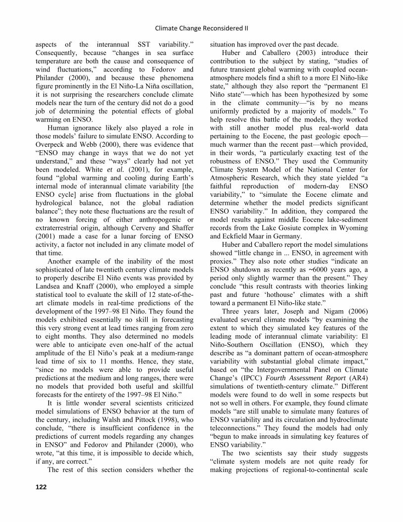
Climate Change Reconsidered II
122
aspects of the interannual SST variability.” Consequently, because “changes in sea surface temperature are both the cause and consequence of wind fluctuations,” according to Fedorov and Philander (2000), and because these phenomena figure prominently in the El Niño-La Niña oscillation, it is not surprising the researchers conclude climate models near the turn of the century did not do a good job of determining the potential effects of global warming on ENSO.
Human ignorance likely also played a role in those models’ failure to simulate ENSO. According to Overpeck and Webb (2000), there was evidence that “ENSO may change in ways that we do not yet understand,” and these “ways” clearly had not yet been modeled. White et al. (2001), for example, found “global warming and cooling during Earth’s internal mode of interannual climate variability [the ENSO cycle] arise from fluctuations in the global hydrological balance, not the global radiation balance”; they note these fluctuations are the result of no known forcing of either anthropogenic or extraterrestrial origin, although Cerveny and Shaffer (2001) made a case for a lunar forcing of ENSO activity, a factor not included in any climate model of that time.
Another example of the inability of the most sophisticated of late twentieth century climate models to properly describe El Niño events was provided by Landsea and Knaff (2000), who employed a simple statistical tool to evaluate the skill of 12 state-of-the-art climate models in real-time predictions of the development of the 1997–98 El Niño. They found the models exhibited essentially no skill in forecasting this very strong event at lead times ranging from zero to eight months. They also determined no models were able to anticipate even one-half of the actual amplitude of the El Niño’s peak at a medium-range lead time of six to 11 months. Hence, they state, “since no models were able to provide useful predictions at the medium and long ranges, there were no models that provided both useful and skillful forecasts for the entirety of the 1997–98 El Niño.”
It is little wonder several scientists criticized model simulations of ENSO behavior at the turn of the century, including Walsh and Pittock (1998), who conclude, “there is insufficient confidence in the predictions of current models regarding any changes in ENSO” and Fedorov and Philander (2000), who wrote, “at this time, it is impossible to decide which, if any, are correct.”
The rest of this section considers whether the
situation has improved over the past decade. Huber and Caballero (2003) introduce their
contribution to the subject by stating, “studies of future transient global warming with coupled ocean-atmosphere models find a shift to a more El Niño-like state,” although they also report the “permanent El Niño state”—which has been hypothesized by some in the climate community—“is by no means uniformly predicted by a majority of models.” To help resolve this battle of the models, they worked with still another model plus real-world data pertaining to the Eocene, the past geologic epoch—much warmer than the recent past—which provided, in their words, “a particularly exacting test of the robustness of ENSO.” They used the Community Climate System Model of the National Center for Atmospheric Research, which they state yielded “a faithful reproduction of modern-day ENSO variability,” to “simulate the Eocene climate and determine whether the model predicts significant ENSO variability.” In addition, they compared the model results against middle Eocene lake-sediment records from the Lake Gosiute complex in Wyoming and Eckfield Maar in Germany.
Huber and Caballero report the model simulations showed “little change in ... ENSO, in agreement with proxies.” They also note other studies “indicate an ENSO shutdown as recently as ~6000 years ago, a period only slightly warmer than the present.” They conclude “this result contrasts with theories linking past and future ‘hothouse’ climates with a shift toward a permanent El Niño-like state.”
Three years later, Joseph and Nigam (2006) evaluated several climate models “by examining the extent to which they simulated key features of the leading mode of interannual climate variability: El Niño-Southern Oscillation (ENSO), which they describe as “a dominant pattern of ocean-atmosphere variability with substantial global climate impact,” based on “the Intergovernmental Panel on Climate Change’s (IPCC) Fourth Assessment Report (AR4) simulations of twentieth-century climate.” Different models were found to do well in some respects but not so well in others. For example, they found climate models “are still unable to simulate many features of ENSO variability and its circulation and hydroclimate teleconnections.” They found the models had only “begun to make inroads in simulating key features of ENSO variability.”
The two scientists say their study suggests “climate system models are not quite ready for making projections of regional-to-continental scale

Global Climate Models and Their Limitations
123
hydroclimate variability and change” and “predicting regional climate variability/change remains an onerous burden on models.”
One year later, L’Ecuyer and Stephens (2007) asked how well state-of-the-art climate models reproduced the workings of real-world energy and water cycles, noting “our ability to model the climate system and its response to natural and anthropogenic forcings requires a faithful representation of the complex interactions that exist between radiation, clouds, and precipitation and their influence on the large-scale energy balance and heat transport in the atmosphere,” further stating “it is also critical to assess [model] response to shorter-term natural variability in environmental forcings using observations.”
The two researchers used multi-sensor observations of visible, infrared, and microwave radiance obtained from the Tropical Rainfall Measuring Mission satellite for the period January 1998 through December 1999 in order to evaluate the sensitivity of atmospheric heating (and the factors that modify it) to changes in east-west SST gradients associated with the strong 1998 El Niño event in the tropical Pacific, as expressed by the simulations of nine general circulation models of the atmosphere utilized in the IPCC’s AR4. This protocol, in their words, “provides a natural example of a short-term climate change scenario in which clouds, precipitation, and regional energy budgets in the east and west Pacific are observed to respond to the eastward migration of warm sea surface temperatures.”
L’Ecuyer and Stephens report “a majority of the models examined do not reproduce the apparent westward transport of energy in the equatorial Pacific during the 1998 El Niño event.” They also discovered “the intermodel variability in the responses of precipitation, total heating, and vertical motion [was] often larger than the intrinsic ENSO signal itself, implying an inherent lack of predictive capability in the ensemble with regard to the response of the mean zonal atmospheric circulation in the tropical Pacific to ENSO.” In addition, they found “many models also misrepresent the radiative impacts of clouds in both regions [the east and west Pacific], implying errors in total cloudiness, cloud thickness, and the relative frequency of occurrence of high and low clouds.” In light of these much-less-than-adequate findings, they conclude, “deficiencies remain in the representation of relationships between radiation, clouds, and precipitation in current climate models,” further
stating these deficiencies “cannot be ignored when interpreting their predictions of future climate.”
Paeth et al. (2008) compared 79 coupled ocean-atmosphere climate simulations derived from 12 different state-of-the-art climate models forced by six IPCC emission scenarios with observational data in order to evaluate how well they reproduced the spatio-temporal characteristics of ENSO over the twentieth century, after which they compared the various models’ twenty-first century simulations of ENSO and the Indian and West African monsoons to one another.
With respect to the twentieth century, this work revealed “all considered climate models draw a reasonable picture of the key features of ENSO.” With respect to the twenty-first century, on the other hand, they note “the differences between the models are stronger than between the emission scenarios,” while “the atmospheric component of ENSO and the West African monsoon are barely affected.” Their “overall conclusion” is that “we still cannot say much about the future behavior of tropical climate.” They consider their study to be merely “a benchmark for further investigations with more recent models in order to document a gain in knowledge or stagnation over the past five years.”
Jin et al. (2008) investigated the overall skill of ENSO prediction in retrospective forecasts made with ten different state-of-the-art ocean-atmosphere coupled general circulation models with respect to their ability to hindcast real-world observations for the 22 years from 1980 to 2001. They found almost all models have problems simulating the mean equatorial SST and its annual cycle. They write, “none of the models we examined attain good performance in simulating the mean annual cycle of SST, even with the advantage of starting from realistic initial conditions.” They also note, “with increasing lead time, this discrepancy gets worse” and “the phase and peak amplitude of westward propagation of the annual cycle in the eastern and central equatorial Pacific are different from those observed.” They also found “ENSO-neutral years are far worse predicted than growing warm and cold events” and “the skill of forecasts that start in February or May drops faster than that of forecasts that start in August or November.” They and others call this behavior “the spring predictability barrier.” Jin et al. conclude, “accurately predicting the strength and timing of ENSO events continues to be a critical challenge for dynamical models of all levels of complexity.”

Climate Change Reconsidered II
124
McLean et al. (2009) quantified “the effect of possible ENSO forcing on mean global temperature, both short-term and long-term,” using Southern Oscillation Index (SOI) data provided by the Australian government’s Bureau of Meteorology. This parameter was defined as “the standardized anomaly of the seasonal mean sea level pressure difference between Tahiti and Darwin, divided by the standard deviation of the difference and multiplied by 10.” The temperature data employed in this endeavor were “the University of Alabama in Huntsville lower-tropospheric (LT) temperature data based on measurements from selected view angles of Microwave Sounding Unit (MSU) channel LT 2” for the period December 1979 to June 2008, supplemented by “balloon-based instrumentation (radiosondes).” For the latter data, dating back to 1958, they employed the Radiosonde Atmospheric Temperature Products for Assessing Climate (RATPAC) product (A) of the U.S. National Climatic Data Center, which represents the atmospheric layer between approximately 1,500 and 9,000 meters altitude.
McLean et al. found “change in SOI accounts for 72% of the variance in GTTA [Global Tropospheric Temperature Anomalies] for the 29-year-long MSU record and 68% of the variance in GTTA for the longer 50-year RATPAC record,” as well as “81% of the variance in tropospheric temperature anomalies in the tropics,” where they note ENSO “is known to exercise a particularly strong influence.” In addition, they determined “shifts in temperature are consistent with shifts in the SOI that occur about 7 months earlier.” The three researchers conclude, “natural climate forcing associated with ENSO is a major contributor to variability and perhaps recent trends in global temperature, a relationship that is not included in current global climate models.”
Harmonic analysis is useful in this discussion because it can be used to construct models of time series or spatial patterns. It also can be used as a diagnostic tool on the same type of data sets. Harmonics are natural solutions to differential equations that represent the motion in oscillating systems and take the form of waves, usually represented as trigonometric functions (for example sine or cosine). Harmonics simply represent the transformation of data from Cartesian coordinates (space and/or time) to a wave coordinate. Thus, “wave-like” phenomena not readily apparent to the eye, or which appear as random noise, can be identified in a data set.
The El Niño (warm East Pacific tropical water temperatures)/La Niña (cold East Pacific tropical water temperatures) phenomenon is known to occur in a quasi-cyclic fashion repeating every two to seven years. It is the leading reason for the global variation in temperatures and precipitation on an interannual time scale. Conceptual models and general circulation models (GCMs) have been used to hypothesize that El Niño may arise as a result of internal nonlinear processes.
White and Liu (2008) found El Niño/La Niña pairs may be “phase locked” to the quasi-decadal oscillation (QDO), which is linked to the 11-year solar cycle. Phase locking means two different harmonics vary in the same way with respect to each other. The simplest example of this is pure “constructive” or “destructive” interference. The authors performed harmonic analysis on a time series of Pacific region sea surface temperatures (SSTs) for 1895–2005. They also gathered 110 years of data from a multi-century run of a coupled atmosphere-ocean GCM corresponding to the observations.
The authors found an 11-year QDO cycle in the observed record as well as strong peaks in the years associated with El Niño, especially at 3.6 and 2.2 years. When the authors ran the GCM without the 11-year solar forcing, the computer model could not reproduce the QDO in its SST record. When the GCM included the forcing, the model not only reproduced the QDO but also the strong peaks in the 3.6 and 2.2 year period similar to observations.
White and Liu also found a “phase locking” of the 11-year cycle with the 3.6 and 2.2 year cycles in both the model and the observations. This suggests the higher frequency oscillations had higher amplitudes in step with the lower frequency one and are “hitting” a maximum (minimum) roughly in correspondence with the low frequency cycle.
White and Liu went further with their analysis, taking the nine 11 year cycles found in each record and “compositing” them (Figure 1.4.1.1). In both the model and observations, similar behavior was observed. When the 11, 3.6, and 2.2 (ridge—warm—El Niño / trough—cold—La Niña) year cycles were added together and superimposed on the 11-year cycle as a visual aid, it was apparent El Niño/La Niña couplets occurred together on the ascending and descending side of the QDO, but that a strong El Niño (La Niña) also can occur at the peak (in the valley) of the QDO.
Finally, White and Liu used the previously derived QDO model of Jin (1997) and incorporated
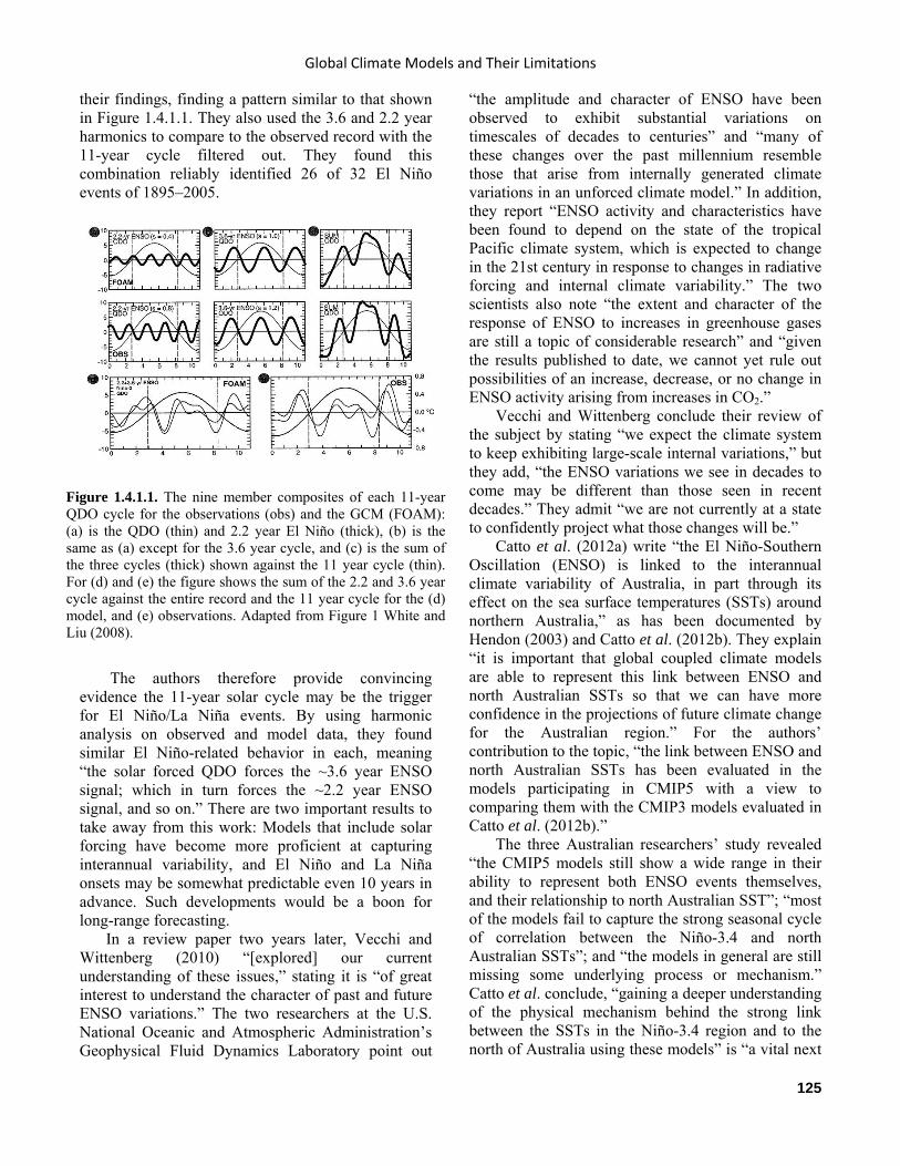
Global Climate Models and Their Limitations
125
their findings, finding a pattern similar to that shown in Figure 1.4.1.1. They also used the 3.6 and 2.2 year harmonics to compare to the observed record with the 11-year cycle filtered out. They found this combination reliably identified 26 of 32 El Niño events of 1895–2005.
The authors therefore provide convincing evidence the 11-year solar cycle may be the trigger for El Niño/La Niña events. By using harmonic analysis on observed and model data, they found similar El Niño-related behavior in each, meaning “the solar forced QDO forces the ~3.6 year ENSO signal; which in turn forces the ~2.2 year ENSO signal, and so on.” There are two important results to take away from this work: Models that include solar forcing have become more proficient at capturing interannual variability, and El Niño and La Niña onsets may be somewhat predictable even 10 years in advance. Such developments would be a boon for long-range forecasting.
In a review paper two years later, Vecchi and Wittenberg (2010) “[explored] our current understanding of these issues,” stating it is “of great interest to understand the character of past and future ENSO variations.” The two researchers at the U.S. National Oceanic and Atmospheric Administration’s Geophysical Fluid Dynamics Laboratory point out
“the amplitude and character of ENSO have been observed to exhibit substantial variations on timescales of decades to centuries” and “many of these changes over the past millennium resemble those that arise from internally generated climate variations in an unforced climate model.” In addition, they report “ENSO activity and characteristics have been found to depend on the state of the tropical Pacific climate system, which is expected to change in the 21st century in response to changes in radiative forcing and internal climate variability.” The two scientists also note “the extent and character of the response of ENSO to increases in greenhouse gases are still a topic of considerable research” and “given the results published to date, we cannot yet rule out possibilities of an increase, decrease, or no change in ENSO activity arising from increases in CO2.”
Vecchi and Wittenberg conclude their review of the subject by stating “we expect the climate system to keep exhibiting large-scale internal variations,” but they add, “the ENSO variations we see in decades to come may be different than those seen in recent decades.” They admit “we are not currently at a state to confidently project what those changes will be.”
Catto et al. (2012a) write “the El Niño-Southern Oscillation (ENSO) is linked to the interannual climate variability of Australia, in part through its effect on the sea surface temperatures (SSTs) around northern Australia,” as has been documented by Hendon (2003) and Catto et al. (2012b). They explain “it is important that global coupled climate models are able to represent this link between ENSO and north Australian SSTs so that we can have more confidence in the projections of future climate change for the Australian region.” For the authors’ contribution to the topic, “the link between ENSO and north Australian SSTs has been evaluated in the models participating in CMIP5 with a view to comparing them with the CMIP3 models evaluated in Catto et al. (2012b).”
The three Australian researchers’ study revealed “the CMIP5 models still show a wide range in their ability to represent both ENSO events themselves, and their relationship to north Australian SST”; “most of the models fail to capture the strong seasonal cycle of correlation between the Niño-3.4 and north Australian SSTs”; and “the models in general are still missing some underlying process or mechanism.” Catto et al. conclude, “gaining a deeper understanding of the physical mechanism behind the strong link between the SSTs in the Niño-3.4 region and to the north of Australia using these models” is “a vital next
Figure 1.4.1.1. The nine member composites of each 11-year QDO cycle for the observations (obs) and the GCM (FOAM): (a) is the QDO (thin) and 2.2 year El Niño (thick), (b) is the same as (a) except for the 3.6 year cycle, and (c) is the sum of the three cycles (thick) shown against the 11 year cycle (thin). For (d) and (e) the figure shows the sum of the 2.2 and 3.6 year cycle against the entire record and the 11 year cycle for the (d) model, and (e) observations. Adapted from Figure 1 White and Liu (2008).

Climate Change Reconsidered II
126
step” for this work, which they state is required “to elucidate the processes missing from the models that cannot capture the link.”
Zhang and Jin (2012) indicate “ENSO behaviors in coupled models have been widely evaluated,” citing Neelin et al. (1992), Delecluse et al. (1998), Latif et al. (2001), Davey et al. (2002), AchuataRao and Sperber (2002, 2006), Capotondi et al. (2006), Guilyardi (2006), and Zhang et al. (2010). However, they write, “coupled models still exhibit large biases in modeling the basic features of ENSO,” citing Guilyardi et al. (2009). Among these biases is “a sea surface temperature (SST) anomaly (SSTA) too tightly confined to the equator (e.g., Stockdale et al., 1998; Kang et al., 2001).” More specifically, and recently, they say, “it was shown that the ENSO meridional width in the models participating in Phase 3 of the Coupled Model Inter-comparison Project (CMIP3) is only about two thirds of what is observed,” citing Zhang et al. (2012).
Zhang and Jin ask the obvious question: “Does the systematical narrow bias in ENSO width still exist in current models developed for Phase 5 of the CMIP (CMIP5)?” They answer the question by assessing the ENSO meridional widths simulated by 15 CMIP5 models and 15 CMIP3 models for the period 1900–1999, comparing the results of both groups against observation-based monthly SST data from the Hadley Center Sea Ice and Sea Surface Temperature (HadISST) data of Rayner et al. (2003).
The analysis indicated “a systematic narrow bias in ENSO meridional width remains in the CMIP5 models,” although they state the newest results represent “a modest improvement over previous models.” Is a modest improvement good enough? That question remains to be answered.
Roxy et al. (2013) point out recent studies have highlighted the existence of a new phenomenon, referred to as the El Niño Modoki, characterized by a warm sea surface temperature (SST) anomaly in the central equatorial Pacific and a cold SST anomaly in the western and eastern Pacific. Some observers of this phenomenon have argued “the increasing frequency of the El Niño Modoki in recent decades is due to global warming.” Roxy et al., considering it imperative to examine the changing teleconnection between ENSO/Modoki and the Indian summer monsoon, revisited “climate change experiments under the fourth Assessment Report (AR4) of the Intergovernmental Panel on Climate Change (IPCC), namely the twentieth century simulations (20C3M) and Special Report on Emissions Scenarios (SRES)
A1B, … to study whether these models can reproduce the ENSO and ENSO Modoki patterns” and “their teleconnections with the Indian summer monsoon, and also the implications for the future.”
The four researchers from India report “only ~1/4th of the models from 20C3M capture either ENSO or ENSO Modoki patterns in June, July, August and September.” They note “of this 1/4th, only two models simulate both ENSO and ENSO Modoki patterns as important modes” and “of these two, only one model simulates both ENSO and ENSO Modoki as important modes during both summer and winter.” In addition, they note the two models that demonstrate ENSO Modoki, as well as ENSO associated variance in both 20C3M and SRES A1B, project the opposite types of impacts of SRES A1B.
Roxy et al. say their findings are indicative of “the challenges associated with the limitations of the models in reproducing the variability of the monsoons and ENSO flavors, not to speak of failing in capturing the potential impacts of global warming as they are expected to.”
Finally, Koumoutsaris (2013) reports, “currently, global climate models disagree in their estimates of feedbacks, and this is one of the main reasons for uncertainty in future climate projections,” citing Bony et al. (2006). He further notes “in order to unveil the origin of these inter-model differences, model simulations need to be evaluated against observations of present climate.”
Koumoutsaris estimated “the feedbacks from water vapor, lapse-rate, Planck, surface albedo and clouds, using models and observations based on the climate response over the last 30 years,” short-term feedbacks that “result both from external changes in the forcing (due to greenhouse gas increases, volcanic and industrial aerosol emissions) and internal climate variations (mostly due to ENSO variability).” The Swiss scientist reports “the CMIP3 models show a much larger interdecile range for all short-term feedbacks in comparison to the long-term ones,” which he states “is also the case for the three models with the most realistic ENSO representation,” citing van Oldenborgh et al. (2005). He also indicates the models have difficulty capturing “the position and magnitude of ENSO teleconnection patterns.” In addition, he reports “the uncertainty in the cloud feedback, using a combination of reanalysis and satellite data, is still very large.”
Koumoutsaris concludes his several analyses indicate “important aspects of the ENSO variability are still poorly understood and/or simulated.”

Global Climate Models and Their Limitations
127
Regarding cloud feedback, he says it is difficult to come to “any firm conclusion,” even as to the sign of the feedback.
Clearly there remain multiple problems in the ability of models to reliably simulate various aspects of climate associated with ENSO events, casting further doubt on the overall ability of models to simulate the future climate of the planet in general. References AchutaRao, K. and Sperber, K.R. 2002. Simulation of the El Niño Southern Oscillation: Results from the Coupled Model Intercomparison Project. Climate Dynamics 19: 191–209.
AchutaRao, K. and Sperber, K.R. 2006. ENSO simulation in coupled ocean-atmosphere models: are the current models better? Climate Dynamics 27: 1–15.
Bony, S., Colman, R., Kattsov, V.M., Allan, R.P., Bretherton, C.S., Dufresne, J., Hall, A., Hallegatte, S., Ingram, W., Randall, D.A., Soden, B.J., Tselioudis, G., and Webb, M.J. 2006. How well do we understand and evaluate climate change feedback processes? Journal of Climate 19: 3445–3482.
Capotondi, A., Wittenberg, A. and Masina, S. 2006. Spatial and temporal structure of tropical Pacific interannual variability in 20th century coupled simulations. Ocean Modeling 15: 274–298.
Catto, J.L., Nicholls, N., and Jakob, C. 2012a. North Australian sea surface temperatures and the El Niño-Southern Oscillation in the CMIP5 models. Journal of Climate 25: 6375–6382.
Catto, J.L., Nicholls, N., and Jakob, C. 2012b. North Australian sea surface temperatures and the El Niño-Southern Oscillation in observations and models. Journal of Climate 25: 5011–5029.
Cerveny, R.S. and Shaffer, J.A. 2001. The moon and El Niño. Geophysical Research Letters 28: 25–28.
Davey, M.K., Huddleston, M., Sperber, K., Braconnot, P., Bryan, F., Chen, D., Colman, R., Cooper, C., Cubasch, U., Delecluse, P., DeWitt, D., Fairhead, L., Flato, G., Gordon, C., Hogan, T., Ji, M., Kimoto, M., Kitoh, A., Knutson, T., Latif, M., LeTreut, H., Li, T., Manabe, S., Mechoso, C., Meehl, G., Power, S., Roeckner, E., Terray, L., Vintzileos, A., Voss, R., Wang, B., Washington, W., Yoshikawa, I., Yu, J., Yukimoto, S., and Zebiak, S. 2002. STOIC: a study of coupled model climatology and variability in tropical ocean regions. Climate Dynamics 18: 403–420.
Delecluse, P., Davey, M.K., Kitamura, Y., Philander, S.G.H., Suarez, M., and Bengtsson, L. 1998. Coupled
general circulation modeling of the tropical Pacific. Journal of Geophysical Research 103: 14,357–14,373.
Fedorov, A.V. and Philander, S.G. 2000. Is El Niño changing? Science 288: 1997–2002.
Guilyardi, E. 2006. El Niño mean state-seasonal cycle interactions in a multi-model ensemble. Climate Dynamics 26: 329–348.
Guilyardi, E., Wittenberg, A., Fedorov, A., Collins, M., Wang, C., Capotondi, A., Jan, G., Oldenborgh, V., and Stockdale, T. 2009. Understanding El Niño in ocean-atmosphere general circulation models: Progress and challenges. Bulletin of the American Meteorological Society 90: 325–340.
Huber, M. and Caballero, R. 2003. Eocene El Niño: Evidence for robust tropical dynamics in the “Hothouse.” Science 299: 877–881.
Jin, E.K., Kinter III, J.L., Wang, B., Park, C.-K., Kang, I.-S., Kirtman, B.P., Kug, J.-S., Kumar, A., Luo, J.-J., Schemm, J., Shukla, J., and Yamagata, T. 2008. Current status of ENSO prediction skill in coupled ocean-atmosphere models. Climate Dynamics 31: 647–664.
Jin, F. F. 1997. An equatorial ocean recharge paradigm for ENSO. Part I: Conceptual Model. Journal of Atmospheric Science 54: 811–829.
Joseph, R. and Nigam, S. 2006. ENSO evolution and teleconnections in IPCC’s twentieth-century climate simulations: Realistic representation? Journal of Climate 19: 4360–4377.
Kang, I.-S., An, S.-I. and Jin, F.-F. 2001. A systematic approximation of the SST anomaly equation for ENSO. Journal of the Meteorological Society of Japan 79: 1–10.
Koumoutsaris, S. 2013. What can we learn about climate feedbacks from short-term climate variations? Tellus A 65: 10.3402/tellusa.v65i0.18887.
Landsea, C.W. and Knaff, J.A. 2000. How much skill was there in forecasting the very strong 1997–98 El Niño? Bulletin of the American Meteorological Society 81: 2107–2119.
Latif, M., Sperber, K., Arblaster, J., Braconnot, P., Chen, D., Colman, A., Cubasch, U., Cooper, C., Delecluse, P., DeWitt, D., Fairhead, L., Flato, G., Hogan, T., Ji, M., Kimoto, M., Kitoh, A., Knutson, T., Le Treut, H., Li, T., Manabe, S., Marti, O., Mechoso, C., Meehl, G., Power, S., Roeckner, E., Sirven, J., Terray, L., Vintzileos, A., Voss, R., Wang, B., Washington, W., Yoshikawa, I., Yu, J., and Zebiak, S. 2001. ENSIP: the El Niño simulation intercomparison project. Climate Dynamics 18: 255–276.
L’Ecuyer, T.S. and Stephens, G.L. 2007. The tropical atmospheric energy budget from the TRMM perspective.

Climate Change Reconsidered II
128
Part II: Evaluating GCM representations of the sensitivity of regional energy and water cycles to the 1998–99 ENSO cycle. Journal of Climate 20: 4548–4571.
McLean, J.D., de Freitas, C.R., and Carter, R.M. 2009. Influence of the Southern Oscillation on tropospheric temperature. Journal of Geophysical Research 114: 10.1029/2008JD011637.
Neelin, J.D., Latif, M., Allaart, M.A.F., Cane, M.A., Cubasch, U., Gates, W.L., Gent, P.R., Ghil, M., Gordon, C., Lau, N.C., Mechoso, C.R., Meehl, G.A., Oberhuber, J.M., Philander, S.G.H., Schopf, P.S., Sperber, K.R., Sterl, K.R., Tokioka, T., Tribbia, J., and Zebiak, S.E. 1992. Tropical air-sea interaction in general circulation models. Climate Dynamics 7: 73–104.
Overpeck, J. and Webb, R. 2000. Nonglacial rapid climate events: Past and future. Proceedings of the National Academy of Sciences USA 97: 1335–1338.
Paeth, H., Scholten, A., Friederichs, P., and Hense, A. 2008. Uncertainties in climate change prediction: El Niño-Southern Oscillation and monsoons. Global and Planetary Change 60: 265–288.
Rayner, N.A., Parker, D.E., Horton, E.B., Folland, C.K., Alexander, L.V., Rowell, D.P., Kent, E.C., and Kaplan, A. 2003. Global analyses of sea surface temperature, sea ice, and night marine air temperature since the late nineteenth century. Journal of Geophysical Research 108: 10.1029/ 2002JD002670.
Roxy, M., Patil, N., Ashok, K., and Aparna, K. 2013. Revisiting the Indian summer monsoon-ENSO links in the IPCC AR4 projections: A cautionary outlook. Global and Planetary Change: 10.1016/j.gloplacha.2013.02.003.
Stockdale, T.N., Busalacchi, A.J., Harrison, D.E., and Seager, R. 1998. Ocean modeling for ENSO. Journal of Geophysical Research 103: 14,325–14,355.
Van Oldenborgh, G.J., Philip, S.Y., and Collins, M. 2005. El Niño in a changing climate: a multi-model study. Ocean Science 1: 81–95.
Vecchi, G.A. and Wittenberg, A.T. 2010. El Niño and our future climate: where do we stand? WIREs Climate Change 1: 10.1002/wcc.33.
Walsh, K. and Pittock, A.B. 1998. Potential changes in tropical storms, hurricanes, and extreme rainfall events as a result of climate change. Climatic Change 39: 199–213.
White, W.B. and Liu, Z. 2008. Non-linear alignment of El Niño to the 11-yr solar cycle. Geophysical Research Letters, 35, L19607, doi:10.1029/2008GL034831.
White, W.B., Cayan, D.R., Dettinger, M.D., and Auad, G. 2001. Sources of global warming in upper ocean temperature during El Niño. Journal of Geophysical
Research 106: 4349–4367.
Zhang, W., Li, J. and Zhao, X. 2010. Sea surface temperature cooling mode in the Pacific cold tongue. Journal of Geophysical Research 115: 10.1029/ 2010JC006501.
Zhang, W. and Jin, F.-F. 2012. Improvements in the CMIP5 simulations of ENSO-SSTA Meridional width. Geophysical Research Letters 39: 10.1029/2012GL053588.
Zhang, W., Jin, F.-F., Li, J., and Zhao, J.-X. 2012. On the bias in simulated ENSO SSTA meridional widths of CMIP3 models. Journal of Climate: org/10.1175/JCLI-D-12-00347.1.
1.4.2 Atlantic and Pacific Ocean Multidecadal Variability (AMV) The study of Semenov et al. (2010) shows natural variability contributed significantly to the warming period in the last few decades of the twentieth century and even may be responsible for the majority of the warming. The work of Petoukhov and Semenov (2010) has been cited as evidence that cold winters would be consistent with anthropogenic global warming. The reasoning follows this path: global warming in the Arctic would leave less sea ice, and with less sea ice, more heat is released to the air. As a result, continents could be colder since more moisture-laden air can mean more clouds and more snow, and thus colder temperatures over land. This is called the “Warm Arctic-Cold Continents” conjecture.
Semenov et al. (2010) first examined the results of several different model experiments performed by others, finding “North Atlantic sea surface temperature changes do project onto Northern Hemisphere and global surface air temperatures in these models,” especially as these relate to the warming of the early twentieth century. They used the ECHAM5 model (European Centre for Medium Range Forecasting general circulation model, at the Max Planck Institute, Hamburg) and ran the model for 80 to 100 years using heat flux patterns (heat transport from the surface into the atmosphere or vice versa) related to the recent positive and negative extremes of the Atlantic Multidecadal Variability (AMV) for three differing regions in the North Atlantic and Arctic.
The authors’ work demonstrated the AMV forced heat fluxes project statistically significant temperature and pressure changes onto the Northern Hemisphere climate, including influencing the NAO. The authors
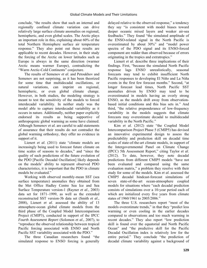
Global Climate Models and Their Limitations
129
conclude, “the results show that such an internal and regionally confined climate variation can drive relatively large surface climate anomalies on regional, hemispheric, and even global scales. The Arctic plays an important role in this, explaining about 60% of the total Northern Hemisphere surface air temperature response.” They also point out these results are applicable to recent decades. However, in their study the forcing of the Arctic on lower latitudes such as Europe is always in the same direction (warmer Arctic means warmer Europe), contradicting the “Warm Arctic-Cold Continents” conjecture.
The results of Semenov et al. and Petoukhov and Semenov are not surprising, as it has been theorized for some time that multidecadal oscillations, or natural variations, can imprint on regional, hemispheric, or even global climate change. However, in both studies, the modeling strategy is meant to test the sensitivity of the models to forced interdecadal variability. In neither study was the model able to capture interdecadal variability as it occurs in nature. Additionally, neither paper explicitly endorsed its results as being supportive of anthropogenic global warming as some have claimed. Although Semenov et al. are careful to add statements of assurance that their results do not contradict the global warming orthodoxy, they offer no evidence in support of it.
Lienert et al. (2011) state “climate models are increasingly being used to forecast future climate on time scales of seasons to decades,” and “since the quality of such predictions of the future evolution of the PDO [Pacific Decadal Oscillation] likely depends on the models’ ability to represent observed PDO characteristics, it is important that the PDO in climate models be evaluated.”
Working with observed monthly-mean SST (sea surface temperature) anomalies they obtained from the Met Office Hadley Centre Sea Ice and Sea Surface Temperature version-1 (Rayner et al., 2003) data set for 1871–1999, as well as the extended reconstructed SST version-3b data set (Smith et al., 2008), Lienert et al. assessed the ability of 13 atmosphere-ocean global climate models from the third phase of the Coupled Model Intercomparison Project (CMIP3), conducted in support of the IPCC Fourth Assessment Report (Solomon et al., 2007), to “reproduce the observed relationship between tropical Pacific forcing associated with ENSO and North Pacific SST variability associated with the PDO.”
The three Canadian researchers found “the simulated response to ENSO forcing is generally
delayed relative to the observed response,” a tendency they say “is consistent with model biases toward deeper oceanic mixed layers and weaker air-sea feedbacks.” They found “the simulated amplitude of the ENSO-related signal in the North Pacific is overestimated by about 30%” and “model power spectra of the PDO signal and its ENSO-forced component are redder than observed because of errors originating in the tropics and extratropics.”
Lienert et al. describe three implications of their findings. First, “because the simulated North Pacific response lags ENSO unrealistically, seasonal forecasts may tend to exhibit insufficient North Pacific responses to developing El Niño and La Niña events in the first few forecast months.” Second, “at longer forecast lead times, North Pacific SST anomalies driven by ENSO may tend to be overestimated in models having an overly strong ENSO, as the models drift away from observation-based initial conditions and this bias sets in.” And third, “the relative preponderance of low-frequency variability in the models suggests that climate forecasts may overestimate decadal to multidecadal variability in the North Pacific.”
Kim et al. (2012) state “the Coupled Model Intercomparison Project Phase 5 (CMIP5) has devised an innovative experimental design to assess the predictability and prediction skill on decadal time scales of state-of-the-art climate models, in support of the Intergovernmental Panel on Climate Change (IPCC) 5th Assessment Report,” citing Taylor et al. (2012). To date, however, they note decadal predictions from different CMIP5 models “have not been evaluated and compared using the same evaluation matrix,” a problem they resolve with their study for some of the models. Kim et al. assessed the CMIP5 decadal hindcast-forecast simulations of seven state-of-the-art ocean-atmosphere coupled models for situations where “each decadal prediction consists of simulations over a 10-year period each of which are initialized every five years from climate states of 1960/1961 to 2005/2006.”
The three U.S. researchers report “most of the models overestimate trends,” in that they “predict less warming or even cooling in the earlier decades compared to observations and too much warming in recent decades.” They also report “low prediction skill is found over the equatorial and North Pacific Ocean” and “the predictive skill for the Pacific Decadal Oscillation index is relatively low for the entire period.” They conclude “the prediction of decadal climate variability against a background of

Climate Change Reconsidered II
130
global warming is one of the most important and challenging tasks in climate science.” References Kim, H.-M., Webster, P.J., and Curry, J.A. 2012. Evaluation of short-term climate change prediction in multi-model CMIP5 decadal hindcasts. Geophysical Research Letters 39: 10.1029/2012GL051644.
Lienert, F., Fyfe, J.C., and Merryfield, W.J. 2011. Do climate models capture the tropical influences on North Pacific sea surface temperature variability? Journal of Climate 24: 6203–6209.
Petoukhov, V. and Semenov, V.A. 2010. A link between reduced Barents-Kara sea ice and cold winter extremes over northern continents. Journal of Geophysical Research—Atmospheres. 115: D21111, doi:10.1029 /2009JD013568.
Rayner, N.A., Parker, D.E., Horton, E.B., Folland, C.K., Alexander, L.V., Rowell, D.P., Kent, E.C., and Kaplan, A. 2003. Global analyses of sea surface temperature, sea ice, and night marine air temperature since the late nineteenth century. Journal of Geophysical Research 108: 10.1029/ 2002JD002670.
Semenov, V.A., Latif, B., Dommenget, D., Keenlyside, N.S., Strehz, A., Martin, T., and Park, W. 2010. The Impact of North Atlantic–Arctic Multidecadal Variability on Northern Hemisphere surface air temperature. Journal of Climate 23: 5668–5677.
Smith, T.M., Reynolds, R.W., Peterson, T.C., and Lawrimore, J. 2008. Improvements to NOAA’s historical merged land-ocean surface temperature analysis (1880–2006). Journal of Climate 21: 2283–2296.
Solomon, S., Qin, D., Manning, M., Marquis, M., Averyt, K., Tignor, M.B., Miller Jr., H.L., and Chen, Z. (Eds.). 2007. Climate Change 2007: The Physical Science Basis. Cambridge University Press, Cambridge, United Kingdom.
Taylor, K.E., Stouffer, R.J., and Meehl, G.A. 2012. An overview of CMIP5 and the experiment design. Bulletin of the American Meteorological Society 93: 485–498.
1.4.3 Intertropical Convergence Zone It is well-known among scientists in the climate modeling community that GCMs erroneously produce a double Intertropical Convergence Zone (ITCZ) in the Central Pacific much more often than is typically observed. The ITCZ is a “belt” of low pressure that girdles the equatorial tropics and identifies the convergence of Earth’s trade wind belts. Usually, a double ITCZ is observed in the Central Pacific during
the Northern Hemisphere spring season only, and not during the rest of the year.
Flaws in the construction of the models, in their numerics and in their physics, are discussed often. But analyses using even erroneous models can sometimes be useful not only in learning where models are deficient but also in identifying where or how the observations need to be improved.
Liu et al. (2012) used the Community Climate System Model version 3 (CCSM3), which includes an atmospheric model, a land surface model, and a dynamic ocean model. The model was of intermediate resolution in the horizontal, the equivalent of 2.8 degrees latitude/longitude. There are 26 model layers in the atmosphere. The authors focused on the first one to two years of the model integration in order to locate the problems causing the double ITCZ over the tropics between 170° E and 150°W. The observed data used as input were archived at the Massachusetts Institute of Technology, and the cloud data were derived from the International Satellite Cloud Climatology Project.
Liu et al. learned warm biases in the sea surface temperatures developed within two years of the initial start-up, and these became substantial and similar to those of other studies after five simulation years. The CCSM model also produced a cold bias south of 10°S. The warm bias was present in all seasons. The effect of the warm and cold bias was to establish unrealistic temperature gradients, which in turn affected the winds and the latent heat flux (moisture) into the atmosphere.
The authors additionally found the warm bias was due to excessive solar radiation, at least at first, augmented by excess latent heating later. The root cause was less cloudiness in the model than was observed in the region. These biases induced errors in the ocean structure of the region studied, resulting in a modeled eastward current where a westward current exists in the observations. An experiment was then run by artificially increasing the cloudiness within the region and the problems described above were alleviated.
Liu et al. eventually traced the problem of insufficient cloudiness in the study region to low cloud liquid water path in the model (Figure 1.4.3.1), but “whether this is due to insufficient absorption of solar radiation in clouds, or insufficient cloud amount or aerosols, is not clear.”
The goal of Liu et al.’s work was to determine how the CCSM model developed a double ITCZ in the Central Pacific. This double Central Pacific ITCZ
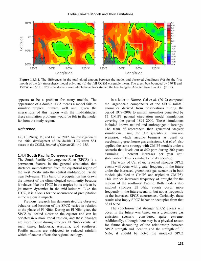
Global Climate Models and Their Limitations
131
appears to be a problem for many models. The appearance of a double ITCZ means a model fails to simulate tropical climate well and, given the interactions of this region with the mid-latitudes, these simulation problems would be felt in the model far from the study region. Reference Liu, H., Zhang, M., and Lin, W. 2012. An investigation of the initial development of the double-ITCZ warm SST biases in the CCSM. Journal of Climate 25: 140–155.
1.4.4 South Pacific Convergence Zone The South Pacific Convergence Zone (SPCZ) is a permanent feature in the general circulation that stretches southeastward from the equatorial region of the west Pacific into the central mid-latitude Pacific near Polynesia. This band of precipitation has drawn the interest of the climatological community because it behaves like the ITCZ in the tropics but is driven by jet-stream dynamics in the mid-latitudes. Like the ITCZ, it is a locus for the occurrence of precipitation in the regions it impacts.
Previous research has demonstrated the observed behavior and location of the SPCZ varies in relation to the phase of El Niño. During an El Niño year, the SPCZ is located closer to the equator and can be oriented in a more zonal fashion, and these changes are more robust during stronger El Niño events. At such times, Indonesia, Australia, and southwest Pacific nations are subjected to reduced rainfall, which of course affects the regional ecology.
In a letter to Nature, Cai et al. (2012) compared the larger-scale components of the SPCZ rainfall anomalies derived from observations during the period 1979–2008 to rainfall anomalies generated by 17 CMIP3 general circulation model simulations covering the period 1891–2000. These simulations included known natural and anthropogenic forcings. The team of researchers then generated 90-year simulations using the A2 greenhouse emission scenarios, which assume business as usual or accelerating greenhouse gas emissions. Cai et al. also applied the same strategy with CMIP5 models under a scenario that levels out at 850 ppm during 200 years assuming 1 percent increases per year until stabilization. This is similar to the A2 scenario.
The work of Cai et al. revealed stronger SPCZ events will occur with greater frequency in the future under the increased greenhouse gas scenarios in both models (doubled in CMIP3 and tripled in CMIP5). This implies increased frequency of drought for the regions of the southwest Pacific. Both models also implied stronger El Niño events occur more frequently in the future scenario, but not as frequently as the increased SPCZ occurrences. Curiously, these results also imply SPCZ behavior decouples from that of El Niño.
The conclusion that stronger SPCZ events will occur in the future was based on a greenhouse gas emission scenario considered quite extreme. Additionally, although there may be a physical reason for future decoupling of the relationship between SPCZ strength and location and the strength of El Niño, it should be noted the modeled SPCZ
Figure 1.4.3.1. The differences in the total cloud amount between the model and observed cloudiness (%) for the first month of the (a) atmospheric model only, and (b) the full CCSM ensemble mean. The green box bounded by 170oE and 150oW and 5° to 10°S is the domain over which the authors studied the heat budgets. Adapted from Liu et al. (2012).

Climate Change Reconsidered II
132
orientation seems to be more zonal than observed even before the future scenarios are generated (compare Figure 1.4.4.1 and Figure 1.4.4.2).
The authors admit to some uncertainty in the observed SPCZ position: “Although the simulated frequency in the control period is comparable to the
Figure 1.4.4.1. The variability of observed rainfall for the (a) spatial pattern of the largest-scale component of the observed precipitation anomalies that was filtered out, and (b) second-largest component of the observed anomalies extracted from the satellite-era rainfall anomaly data (mm d-1) (Global Precipitation Climatology Project version 225) focusing on the western South Pacific during the austral summer (December to February). The first (second) principal patterns account for 47% (16%) of the total variance. The SPCZ position (max rainfall greater than 6mm d-1) for El Niño (green line), La Niña (blue line), and neutral (black line) states is superimposed in a, and the position for zonal SPCZ events (red line) in b. Cold (warm) contours indicate increased (decreased) rainfall per one standard deviation (s.d.) change. Adapted from Figure 1 in Cai et al. (2012).
Figure 1.4.4.2. As in Figure 1.5.4.1, except for the CMIP model runs.

Global Climate Models and Their Limitations
133
observed frequency, the latter is based on observations over some three decades and may carry a large uncertainty.” Like many modeling studies, the outcome of Cai et al. is properly understood as nothing more than a scenario based on a specific set of assumptions, with limitations on the ability to capture the phenomenon in question precisely. Their results have only limited scientific value. Reference Cai, W., Langaigne, M., Borlace, S., Collins, M., Cowan, T., McPhadden, M.J., Timmermann, A., Power, S., Brown, J., Menkes, C., Ngari, A., Vincent, E.M. and Widlansky, M.J. 2012. More extreme swings of the South Pacific Convergence Zone due to greenhouse warming. Nature 488: 365-369.
1.4.5 Hadley Circulation The Hadley Circulation, or Hadley Cell, is an important general circulation of Earth’s climate. It is named for Sir George Hadley, who first attempted to describe Earth’s circulation in a general way. Warm equatorial air rises, while cold polar air sinks, and a hemisphere-wide circulation loop is formed. Hadley was partly correct but failed to account for the Coriolis Effect, which was discovered by later researchers.
The Hadley Cell emerges from an analysis of the tropics when atmospheric motions are averaged on the time scale of a month or more. In a classical view of this circulation, there are upward motions and low pressure at the equator (mainly associated with deep convection clouds), poleward moving air aloft, downward motion around 30o latitude, associated with the subtropical highs, and equatorward moving air (the trade winds) in the lower atmosphere. Studies have suggested the latitudinal extent of the Hadley Cell may have widened in the past few decades.
Levine and Schneider (2011) used a crude atmospheric general circulation model to examine the strength and span of the HC over a wide range of climates. They performed this study because some studies show the HC strengthens, while others show it weakens, in response to global warming. As Levine and Schneider report in describing the rationale behind their study, “despite a large body of observations and numerous studies with GCMs, it remains unclear how the width and strength of the Hadley Circulation are controlled.”
Levine and Schneider used an idealized radiative transfer scheme and moist thermodynamics. The
model was based on one used at the Geophysical Fluid Dynamics Laboratory, a model with relatively coarse resolution (about 2.8° latitude/longitude) and 30 levels in the vertical. The planet “surface” was water-covered only. The oceans included simple dynamics for heat transport (which was turned “on” and “off”), and the model was driven with the annual mean insolation, thus there was no diurnal or annual cycle. In this way the authors could isolate two variables, the strength of the HC versus global temperature (controlled by the absorption of longwave radiation only).
The authors established a baseline climate for their aqua-planet and ran the model with and without ocean dynamics. The results were more realistic with the ocean dynamics. Then, the longwave absorption, a function of latitude and pressure (height), was varied by a constant amount between 0.2 and 6.0 times the control value. This produced a global climate with planetary temperatures varying between 260 K and 315 K (roughly -13°C to 42°C; today it is roughly 15°C). The equator-to-pole temperature differences decreased linearly with increasing temperature.
In their simulations, the strength of the Hadley Cell did not change linearly (Figure 1.4.5.1) but rather was more parabolic in shape, which makes the situation more complicated. The Hadley Circulation in their model was weaker in both very cold and very warm climates. Also, Figure 1.4.5.1 implies ocean dynamics become less important in determining the strength of the Hadley Circulation as climate warms. This is true because the equator-to-pole temperature difference becomes negligible. In colder climates, the weakening is the result of a more geostrophic, or zonal, atmospheric flow. A more zonal flow would imply less wave action in the jet stream, which means less energy exchange. Today’s climate is roughly at the maximum in the ocean dynamics curve.
The behavior of atmospheric systems can be complicated even when there are few variables. This has led to studies whose findings initially seem to be contradictory, for example, in a warmer climate. The behavior of changes in the strength of the Hadley Circulation is nonlinear even in the simple model of Levine and Schneider (2011). Adding complexity to the model would make interpretation of the output more difficult. This demonstrates the importance of understanding the fundamental behavior of phenomena like the Hadley Circulation.
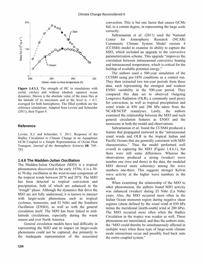
Climate Change Reconsidered II
134
Reference Levine, X.J. and Schneider, T. 2011. Response of the Hadley Circulation to Climate Change in an Aquaplanet GCM Coupled to a Simple Representation of Ocean Heat Transport. Journal of the Atmospheric Sciences 68: 769–783.
1.4.6 The Madden-Julian Oscillation The Madden-Julian Oscillation (MJO) is a tropical phenomenon discovered in the early 1970s; it is a 30- to 70-day oscillation in the west-to-east component of the tropical winds between 20°N and 20°S. The MJO has been detected in tropical convection and precipitation, both of which are enhanced in the “trough” phase. Although the dynamics that drive the MJO are not fully understood, it is known to interact with larger-scale phenomena such as tropical cyclones, monsoons, and El Niño and the Southern Oscillation (ENSO), as well as with the general circulation itself. The MJO has been linked to mid-latitude circulations, especially during the warm season and over North America.
General circulation models have had difficulty in representing the MJO and its impact on larger-scale phenomena could not be captured, due primarily to the inadequate representation of the associated
convection. This is but one factor that causes GCMs fail, to a certain degree, in representing the large scale correctly.
Subramanian et al. (2011) used the National Center for Atmospheric Research (NCAR) Community Climate System Model version 4 (CCSM4) model to examine its ability to capture the MJO, which included an upgrade to the convective parameterization scheme. This upgrade “improves the correlation between intraseasonal convective heating and intraseasonal temperature, which is critical for the buildup of available potential energy.”
The authors used a 500-year simulation of the CCSM4 using pre-1850 conditions as a control run. They then extracted two ten-year periods from these data, each representing the strongest and weakest ENSO variability in the 500-year period. They compared this data set to observed Outgoing Longwave Radiation (OLR), a commonly used proxy for convection, as well as tropical precipitation and zonal winds at 850 and 200 hPa taken from the NCAR/NCEP reanalyses. Lastly, the authors examined the relationship between the MJO and such general circulation features as ENSO and the monsoons in both the model and observations.
Subramanian et al. found the CCSM4 produced a feature that propagated eastward in the “intraseasonal zonal winds and OLR in the tropical Indian and Pacific Oceans that are generally consistent with MJO characteristics.” Thus the model performed well overall in capturing the MJO (Figure 1.4.6.1), but there were still some differences. Whereas the observations produced a strong (weaker) wave number one (two and three) in the data, the modeled MJO showed more coherency among the wave numbers one-three. This suggests stronger Kelvin wave activity at the higher wave numbers in the model.
When examining the relationship of the MJO to other phenomenon, the authors found MJO activity was enhanced (weaker) during El Niño (La Niña) years. Also, the MJO occurred more often in the Indian Ocean monsoon region during negative shear regimes (shear defined by the zonal wind at 850 hPa minus the meridional [north-south] wind at 200 hPa). The MJO occurred more often when the Hadley Circulation in the tropics was weaker as well. These phenomena are interrelated, and thus the authors state, the “MJO could thereby be simultaneously affected in multiple ways when these type of large-scale climate mode interactions occur and possibly feed back onto the entire coupled system.”
Figure 1.4.5.1. The strength of HC in simulations with (solid, circles) and without (dashed, squares) ocean dynamics. Shown is the absolute value of the mass flux at the latitude of its maximum and at the level σc = 0.7, averaged for both hemispheres. The filled symbols are the reference simulations. Adapted from Levine and Schneider (2011), their Figure 4.
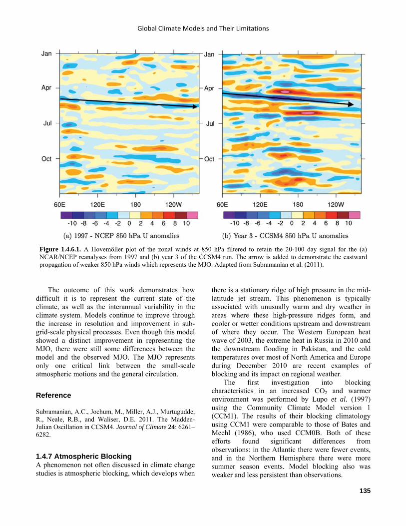
Global Climate Models and Their Limitations
135
The outcome of this work demonstrates how difficult it is to represent the current state of the climate, as well as the interannual variability in the climate system. Models continue to improve through the increase in resolution and improvement in sub-grid-scale physical processes. Even though this model showed a distinct improvement in representing the MJO, there were still some differences between the model and the observed MJO. The MJO represents only one critical link between the small-scale atmospheric motions and the general circulation.
Reference Subramanian, A.C., Jochum, M., Miller, A.J., Murtugudde, R., Neale, R.B., and Waliser, D.E. 2011. The Madden-Julian Oscillation in CCSM4. Journal of Climate 24: 6261–6282.
1.4.7 Atmospheric Blocking A phenomenon not often discussed in climate change studies is atmospheric blocking, which develops when
there is a stationary ridge of high pressure in the mid-latitude jet stream. This phenomenon is typically associated with unusually warm and dry weather in areas where these high-pressure ridges form, and cooler or wetter conditions upstream and downstream of where they occur. The Western European heat wave of 2003, the extreme heat in Russia in 2010 and the downstream flooding in Pakistan, and the cold temperatures over most of North America and Europe during December 2010 are recent examples of blocking and its impact on regional weather.
The first investigation into blocking characteristics in an increased CO2 and warmer environment was performed by Lupo et al. (1997) using the Community Climate Model version 1 (CCM1). The results of their blocking climatology using CCM1 were comparable to those of Bates and Meehl (1986), who used CCM0B. Both of these efforts found significant differences from observations: in the Atlantic there were fewer events, and in the Northern Hemisphere there were more summer season events. Model blocking also was weaker and less persistent than observations.
Figure 1.4.6.1. A Hovemöller plot of the zonal winds at 850 hPa filtered to retain the 20-100 day signal for the (a) NCAR/NCEP reanalyses from 1997 and (b) year 3 of the CCSM4 run. The arrow is added to demonstrate the eastward propagation of weaker 850 hPa winds which represents the MJO. Adapted from Subramanian et al. (2011).
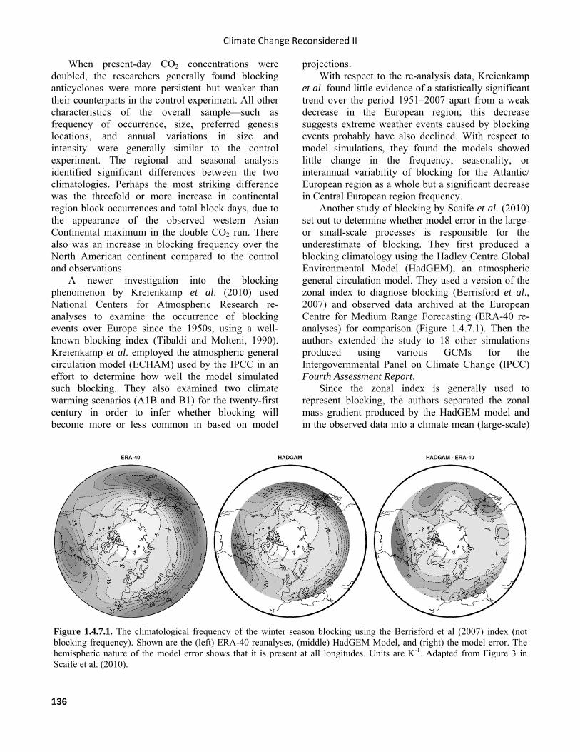
Climate Change Reconsidered II
136
When present-day CO2 concentrations were doubled, the researchers generally found blocking anticyclones were more persistent but weaker than their counterparts in the control experiment. All other characteristics of the overall sample—such as frequency of occurrence, size, preferred genesis locations, and annual variations in size and intensity—were generally similar to the control experiment. The regional and seasonal analysis identified significant differences between the two climatologies. Perhaps the most striking difference was the threefold or more increase in continental region block occurrences and total block days, due to the appearance of the observed western Asian Continental maximum in the double CO2 run. There also was an increase in blocking frequency over the North American continent compared to the control and observations.
A newer investigation into the blocking phenomenon by Kreienkamp et al. (2010) used National Centers for Atmospheric Research re-analyses to examine the occurrence of blocking events over Europe since the 1950s, using a well-known blocking index (Tibaldi and Molteni, 1990). Kreienkamp et al. employed the atmospheric general circulation model (ECHAM) used by the IPCC in an effort to determine how well the model simulated such blocking. They also examined two climate warming scenarios (A1B and B1) for the twenty-first century in order to infer whether blocking will become more or less common in based on model
projections. With respect to the re-analysis data, Kreienkamp
et al. found little evidence of a statistically significant trend over the period 1951–2007 apart from a weak decrease in the European region; this decrease suggests extreme weather events caused by blocking events probably have also declined. With respect to model simulations, they found the models showed little change in the frequency, seasonality, or interannual variability of blocking for the Atlantic/ European region as a whole but a significant decrease in Central European region frequency.
Another study of blocking by Scaife et al. (2010) set out to determine whether model error in the large- or small-scale processes is responsible for the underestimate of blocking. They first produced a blocking climatology using the Hadley Centre Global Environmental Model (HadGEM), an atmospheric general circulation model. They used a version of the zonal index to diagnose blocking (Berrisford et al., 2007) and observed data archived at the European Centre for Medium Range Forecasting (ERA-40 re-analyses) for comparison (Figure 1.4.7.1). Then the authors extended the study to 18 other simulations produced using various GCMs for the Intergovernmental Panel on Climate Change (IPCC) Fourth Assessment Report.
Since the zonal index is generally used to represent blocking, the authors separated the zonal mass gradient produced by the HadGEM model and in the observed data into a climate mean (large-scale)
Figure 1.4.7.1. The climatological frequency of the winter season blocking using the Berrisford et al (2007) index (not blocking frequency). Shown are the (left) ERA-40 reanalyses, (middle) HadGEM Model, and (right) the model error. The hemispheric nature of the model error shows that it is present at all longitudes. Units are K-1. Adapted from Figure 3 in Scaife et al. (2010).
Global Climate Models and Their Limitations
137
component versus that of the time-varying portion (small-scale). When they replaced the large-scale model data with the observed (keeping the small-scale model part), they showed the blocking frequency was reproduced more faithfully. The same result was found in the IPCC simulations and by Lupo et al. (1997).
Scaife et al. state, “commonly applied statistics based on absolute measures (such as the reversal of the geopotential height or potential vorticity gradients) show large errors in current climate models, but these are directly attributable to a large degree to errors in the main state.” Scaife et al. also show improvements in the large-scale model performance can greatly improve the capability of the model to reproduce blocking characteristics.
The latest study by Mokhov et al. (2013) for the projection of blocking in the twenty-first century using the Institut Pierre Simon Laplace Climate Model versions 4 (IPSL-CM4) GCM and the SRES-A1B and SRES-A2 scenarios showed a slight increase in the number and persistence of blocking events over the Atlantic-Eurasian region and no change in the interannual or interdecadal variability. These results are similar to the other studies examined here.
Although caution should be emphasized in interpreting the model projections, the findings of these studies are good news, for they suggest the number of heat waves and/or cold waves that can be attributed to atmospheric blocking will not increase for the Atlantic/European region in the twenty-first century. In fact, the model output suggests fewer of these occurrences and/or a shorter duration of such events (e.g., Kreiencamp et al., 2010).
Studies by Liu et al. (2012) and Jaiser et al. (2012) find an increase in observed blocking since 1995 consistent with that found by Mokhov et al. (2013), but rather than linking this to internal variability, including changes in the phases of multidecadal oscillations, they attribute the change to anthropogenic climate warming. A paper by Hakkinen et al. (2011) takes a more measured approach, stating, “the warm-ocean/cold-land anomaly pattern has been linked to a dynamical environment favorable for blocking” and “the possibility of coupled interaction of atmosphere with [Atlantic Multidecadal Variability] seems likely, given the long-period variability of blocking reported here and in the even longer paleoclimate time series.” The latter position is more consistent with the studies reviewed here.
Two studies provide additional evidence for the
the lack of trends in Northern Hemisphere blocking patterns. Screen and Simmonds (2013) studied “observed changes (1979–2011) in atmospheric planetary-wave amplitude over northern mid-latitudes, which have been proposed as a possible mechanism linking Arctic Amplification (AA) and mid-latitude weather extremes.” However, they found few if any large or statistically significant changes, instead noting “Statistically significant changes in either metric are limited to few seasons, wavelengths and longitudinal sectors” and “Even ignoring the lack of significance, there is no clear tendency towards larger or smaller [wave amplitude] (60% negative trends and 40% positive trends). Nor is there a general tendency towards longer or shorter wavelengths (i.e., longer wavelengths are not increasing in zonal amplitude at the expense of shorter wavelengths), or vice versa.”
Most recently, Barnes (2013) investigated “trends in the meridional extent of atmospheric waves over North America and the North Atlantic … in three reanalyses.” Barnes’s work “demonstrated that previously reported positive trends are an artifact of the methodology” and further “the mechanism put forth by previous studies (e.g. Francis and Vavrus [2012]; Liu et al. [2012]), that amplified polar warming has led to the increased occurrence of slow-moving weather patterns and blocking episodes, is unsupported by the observations.”
One of the criticisms of model projections used to produce climate change scenarios for the twenty-first century is that the models still have difficulty reproducing various aspects of the observed climate, including even the large-scale features (Scaife et al., 2010). Blocking is one of these phenomena, and it is often used as a surrogate for the occurrence of extreme conditions (heat waves, cold waves). If the models cannot adequately represent blocking in the current climate, results regarding the occurrence of extreme events in future climate change scenarios must be examined with caution.
References Barnes, E. 2013. Revisiting the evidence linking Arctic Amplification to extreme weather in the midlatitude. Geophysical Research Letters, in press: 10.1002/grl.50880.
Bates, G.T. and Meehl, G.A. 1986. The effect of CO2 concentration on the frequency of blocking in a general circulation model coupled to a single mixed layer ocean model. Monthly Weather Review 114: 687–701.

Climate Change Reconsidered II
138
Berrisford, P., Hoskins, B.J., and Tyrlis, E. 2007. Blocking and Rossby wave breaking on the dynamical tropopause in the Southern Hemisphere. Journal of Atmospheric Science 64: 288–-2898.
Francis, J.A. and Vavrus, S.J. 2012. Evidence linking Arctic amplification to extreme weather in mid-latitudes. Geophysical Research Letters 39: 10.1029/ 2012GL051000. Hakkinen, S., Rhines, P.B., and Worthen, D.L. 2011. Atmospheric blocking and Atlantic Multidecadal Ocean Variability. Science 334: 655–659.
Jaiser, R., Dethloff, K., Handorf, D., Rinke, A., and Cohen, J. 2012. Impact of sea ice cover changes on the Northern Hemisphere atmospheric winter circulation. Tellus A 64: 11595, DOI: 10.3402/tellusa.v64i0.11595.
Kreienkamp, F., Spekat, A., and Enke, W. 2010. Stationarity of atmospheric waves and blocking over Europe—based on a reanalysis dataset and two climate scenarios. Theory of Applied Climatology 102: 205–212.
Liu, J., Curry, J.A., Wang, H., Song, M., and Horton, R.M. 2012. Impact of declining Arctic sea ice on winter snowfall. Proceedings of the National Academy of Sciences 109: 6781–6783.
Lupo, A.R., Oglesby, R.J., and Mokhov, I.I. 1997. Climatological features of blocking anticyclones: A study of Northern Hemisphere CCM1 model blocking events in present-day and double CO2 atmospheres. Climate Dynamics 13: 181–195.
Mokhov, I.I., Akperov, M.G., Prokofyeva, M.A., Timazhev, A.V., Lupo, A.R., and Le Treut, H. 2013. Blockings in the Northern Hemisphere and Euro-Atlantic Region: Estimates of changes from reanalysis data and model simulations. Doklady Earth Sciences 449: 430–433.
Scaife, A.A., Wollings, T., Knight, J., Martin G., and Hinton, T. 2010. Atmospheric blocking and mean biases in climate models. Journal of Climate 23: 6143–6152.
Screen, J. and Simmonds, I. 2013. Exploring links between Arctic amplification and midlatitude weather. Geophysical Research Letters 40: 10.1002/GRL.50174.
Tibaldi, S. and Molteni, F. 1990. On the operational predictability of blocking. Tellus 42A: 343–365.
1.4.8 Tropical Cyclones Tropical cyclones (TCs) form and are maintained by the cooperative forcing between the atmosphere and oceans. Warm tropical waters (sea surface temperatures or SSTs) are the energy source needed to generate and maintain them, but favorable
atmospheric conditions (e.g., low wind shear) are just as critical. These atmospheric conditions can be correlated to warm tropical SSTs. But warmer SSTs by themselves do not always portend more TCs. Some general circulation model studies have projected there will be as much as a 200 percent increase in TC occurrence in a warmer world, while other GCM studies suggest such a world will bring fewer TCs.
Villarini et al. (2011) attempted to explain why there is a large spread in the projection of TC occurrences that may occur in the future. They used a statistical model trained using a 131-year record of North Atlantic TC occurrences, a Poisson regression type model that generated land-falling or Atlantic TC frequencies as a function of Atlantic region and/or tropical mean SSTs. The SSTs included variability related to the North Atlantic Oscillation (interdecadal) and the Southern Oscillation Index (interannual). The authors compared the statistical model results with those produced by dynamic GCMs and statistical-dynamic models for the Intergovernmental Panel on Climate Change (IPCC). In order for the comparisons to be more faithful, the authors used the SST time series in the statistical model that each particular IPCC model scenario used.
When both the Atlantic region and tropical mean SSTs were used, there was good agreement between the results of the statistical model and that of the dynamic models (Figure 1.4.8.1). Tropical SSTs elsewhere can affect Atlantic TC occurrence via variations in the jet stream. The authors note, “the agreement between the statistical and dynamical models is rather remarkable, considering the simplicity of the statistical model.” They also state “it appears that the differences among the published results can be largely reduced to differences in the climate model projections of tropical Atlantic SST changes relative to the global tropics used by the studies.”
When Villarini et al. used Atlantic SST alone, there was little agreement between the statistical and dynamic models, with the statistical models showing large biases in TC frequency. The dynamic models did not show this bias, supporting the notion that SSTs alone cannot explain variations in TC occurrence. There were also mixed signals produced by the IPCC models with regard to landfalling TCs, half showing a statistically significant increase and the other half showing a significant decrease. The authors suggest that in order to reduce the uncertainty in future TC occurrence, the uncertainty in tropical
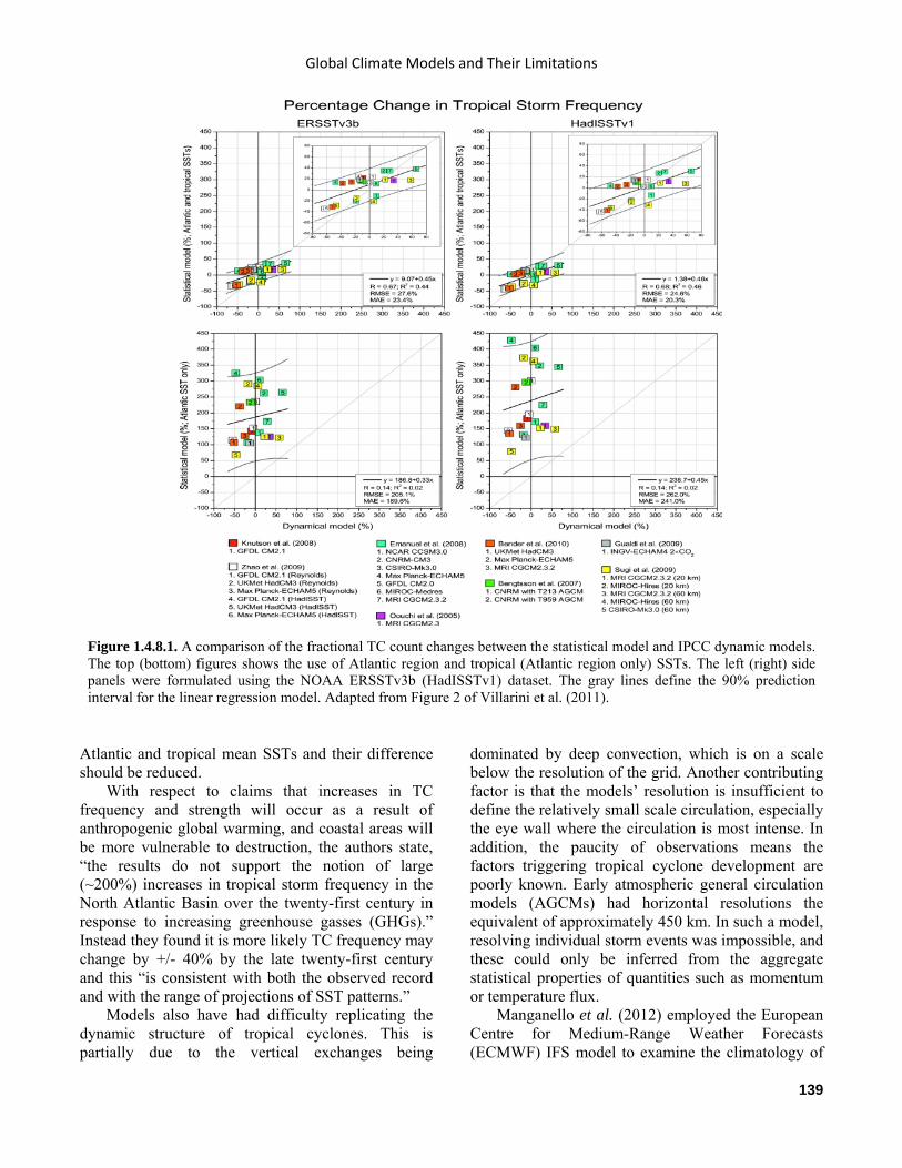
Global Climate Models and Their Limitations
139
Atlantic and tropical mean SSTs and their difference should be reduced.
With respect to claims that increases in TC frequency and strength will occur as a result of anthropogenic global warming, and coastal areas will be more vulnerable to destruction, the authors state, “the results do not support the notion of large (~200%) increases in tropical storm frequency in the North Atlantic Basin over the twenty-first century in response to increasing greenhouse gasses (GHGs).” Instead they found it is more likely TC frequency may change by +/- 40% by the late twenty-first century and this “is consistent with both the observed record and with the range of projections of SST patterns.”
Models also have had difficulty replicating the dynamic structure of tropical cyclones. This is partially due to the vertical exchanges being
dominated by deep convection, which is on a scale below the resolution of the grid. Another contributing factor is that the models’ resolution is insufficient to define the relatively small scale circulation, especially the eye wall where the circulation is most intense. In addition, the paucity of observations means the factors triggering tropical cyclone development are poorly known. Early atmospheric general circulation models (AGCMs) had horizontal resolutions the equivalent of approximately 450 km. In such a model, resolving individual storm events was impossible, and these could only be inferred from the aggregate statistical properties of quantities such as momentum or temperature flux.
Manganello et al. (2012) employed the European Centre for Medium-Range Weather Forecasts (ECMWF) IFS model to examine the climatology of
Figure 1.4.8.1. A comparison of the fractional TC count changes between the statistical model and IPCC dynamic models. The top (bottom) figures shows the use of Atlantic region and tropical (Atlantic region only) SSTs. The left (right) side panels were formulated using the NOAA ERSSTv3b (HadISSTv1) dataset. The gray lines define the 90% prediction interval for the linear regression model. Adapted from Figure 2 of Villarini et al. (2011).

Climate Change Reconsidered II
140
TCs by identifying individual events. This model is the recent version of the ECMWF GCM and includes the latest physical packages for cloud formation (i.e., prognostic equations for cloud water), land surface processes and hydrology, and improved convective adjustment schemes. The latter provided for a better representation of tropical weather and year-to-year variations in tropical climate.
The model was run for “Project Athena” (Jung et al., 2012) with resolutions at 125 km, 39 km, 16 km (the current resolution of a weather forecast model), and 10 km; for all there were 91 levels in the vertical. The model also was run for each year from 1960 to 2008 for the larger resolutions, and for 1989–2008 for the 10 km run. To keep the data storage manageable, the authors used data for May through November in the Northern Hemisphere (NH) for 1990–2008. The authors also controlled the data to make sure storms identified were indeed TCs, such as requiring a warm core, meaning the center is warmer than the surrounding environment.
Manganello et al. found over the entire NH, the 39 km run produced the most realistic count for TCs; the higher resolution model produced too many TCs. Within each basin (e.g., Atlantic) or sub-basin (Northwest Pacific), however, the higher resolutions occasionally produced the best results. One problem for models is tropical cyclogenesis tends to be too weak, and it was a problem here in spite of better resolution. In a related matter, the model produced TCs that were weaker than observed in terms of wind speed but comparable in terms of central pressure (Figure 1.4.8.2). Finally, the higher model resolution runs did better in capturing ENSO variability of TCs. ENSO is well-known to have a large influence on the interannual variation of TC occurrence and intensity.
Manganello et al. note, “as computing power continues to grow, it is becoming increasingly possible to model the global climate at horizontal resolutions presently used in short-term weather prediction.” Although hindcasts with improved resolution and physics still have difficulty representing observations to a high degree, the models are able to reasonably reproduce the number of events, and even produced structures that look like observed TCs (Figure 1.4.8.3), thus, passing the test. These kinds of advances represent progress and should make future computer scenarios for climate more reasonable and useful.
The studies of Dare and McBride (2011) and Park et al. (2011) have demonstrated tropical cyclones (TCs) can significantly cool the surface waters in
their wakes for periods of several days to weeks. Manucharyan et al. (2011) write, “TC-induced ocean mixing can have global climate impacts as well, including changes in poleward heat transport, ocean circulation, and thermal structure.” They note, however, that “in several previous modeling studies devoted to this problem, the TC mixing was treated as a permanent (constant in time) source of additional vertical diffusion in the upper ocean.” They thus explore the “highly intermittent character of the mixing” and what it portends for global climate, using a global ocean-atmosphere coupled model and a simple heat transfer model of the upper ocean.
The three Yale University researchers mimicked the effects of TCs using several representative cases of time-dependent mixing that yield the same annual mean values of vertical diffusivity, conforming with the studies of Jansen and Ferrari (2009) and Fedorov et al. (2010), wherein spatially uniform (but varying
Figure 1.4.8.2. Life cycle composite of the (a) maximum 10-m wind speed and (b) minimum SLP for the 25 most intense typhoons, in terms of the maximum 10-m wind speed, over the northwest Pacific for observed data (black), the 10-km (purple), the 16-km (red), and 39-km (green) runs during MJJASON of 1990–2008. The time step is in 6-h increments. Adapted from Figure 9, Manganello et al. (2012).
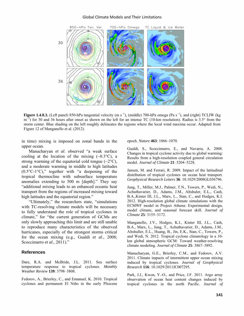
Global Climate Models and Their Limitations
141
in time) mixing is imposed on zonal bands in the upper ocean.
Manucharyan et al. observed “a weak surface cooling at the location of the mixing (~0.3°C), a strong warming of the equatorial cold tongue (~2°C), and a moderate warming in middle to high latitudes (0.5°C-1°C),” together with “a deepening of the tropical thermocline with subsurface temperature anomalies extending to 500 m [depth].” They say “additional mixing leads to an enhanced oceanic heat transport from the regions of increased mixing toward high latitudes and the equatorial region.”
“Ultimately,” the researchers state, “simulations with TC-resolving climate models will be necessary to fully understand the role of tropical cyclones in climate,” for “the current generation of GCMs are only slowly approaching this limit and are still unable to reproduce many characteristics of the observed hurricanes, especially of the strongest storms critical for the ocean mixing (e.g., Gualdi et al., 2008; Scoccimarro et al., 2011).” References Dare, R.A. and McBride, J.L. 2011. Sea surface temperature response to tropical cyclones. Monthly Weather Review 139: 3798–3808.
Fedorov, A., Brierley, C., and Emanuel, K. 2010. Tropical cyclones and permanent El Niño in the early Pliocene
epoch. Nature 463: 1066–1070.
Gualdi, S., Scoccimarro, E., and Navarra, A. 2008. Changes in tropical cyclone activity due to global warming: Results from a high-resolution coupled general circulation model. Journal of Climate 21: 5204–5228.
Jansen, M. and Ferrari, R. 2009. Impact of the latitudinal distribution of tropical cyclones on ocean heat transport. Geophysical Research Letters 36: 10.1029/2008GL036796.
Jung, T., Miller, M.J., Palmer, T.N., Towers, P., Wedi, N., Achuthavarier, D., Adams, J.M., Altshuler, E.L., Cash, B.A.,Kinter III, J.L., Marx, L., Stan, C., and Hodges, K.I. 2012. High-resolution global climate simulations with the ECMWF model in Project Athena: Experimental design, model climate, and seasonal forecast skill. Journal of Climate 25: 3155–3172.
Manganello, J.V., Hodges, K.I., Kinter III, J.L., Cash, B.A., Marx, L., Jung, T., Achuthavarier, D., Adams, J.M., Altshuller, E.L., Huang, B., Jin, E.K., Stan, C., Towers, P., and Wedi, N. 2012. Tropical cyclone climatology in a 10-km global atmospheric GCM: Toward weather-resolving climate modeling. Journal of Climate 25: 3867–3892.
Manucharyan, G.E., Brierley, C.M., and Fedorov, A.V. 2011. Climate impacts of intermittent upper ocean mixing induced by tropical cyclones. Journal of Geophysical Research 116: 10.1029/2011JC007295.
Park, J.J., Kwon, Y.-O., and Price, J.F. 2011. Argo array observation of ocean heat content changes induced by tropical cyclones in the north Pacific. Journal of
Figure 1.4.8.3. (Left panel) 850-hPa tangential velocity (m s−1), (middle) 700-hPa omega (Pa s−1), and (right) TCLIW (kg m−2) for 30 and 36 hours after onset as shown on the left for an intense TC (10-km resolution). Radius is 3.5° from the storm center. Blue shading on the left roughly delineates the regions where the local wind maxima occur. Adapted from Figure 12 of Manganello et al. (2012).
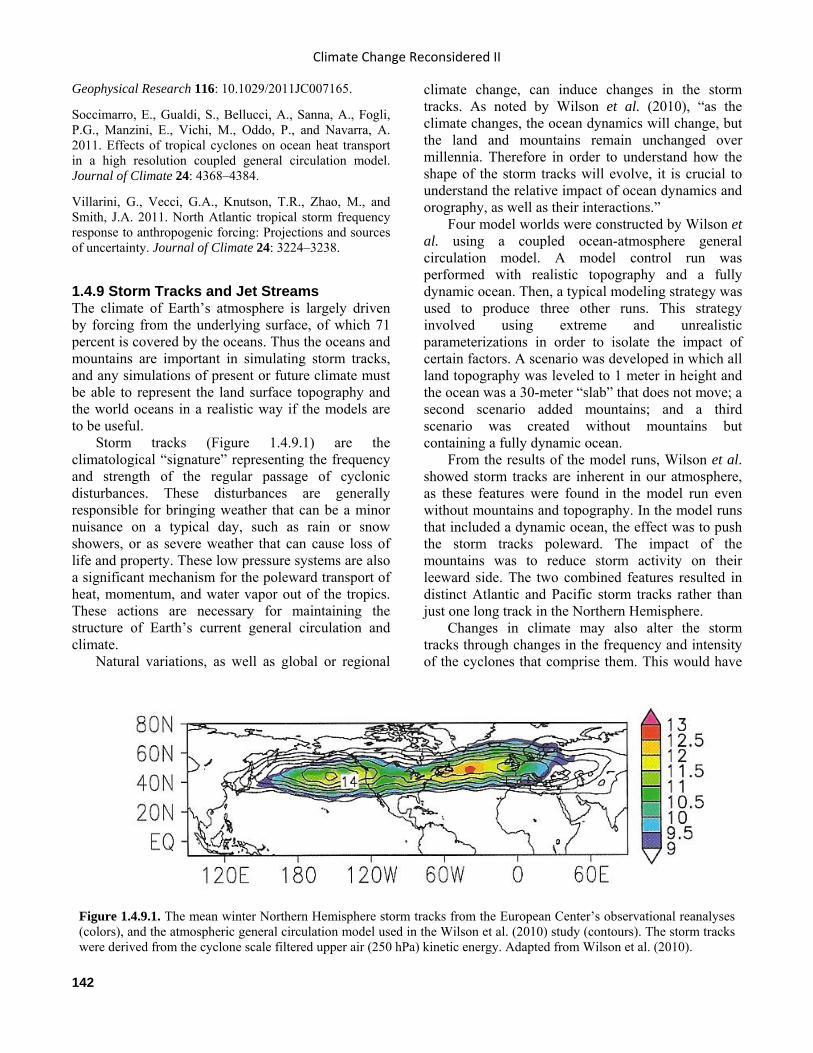
Climate Change Reconsidered II
142
Geophysical Research 116: 10.1029/2011JC007165.
Soccimarro, E., Gualdi, S., Bellucci, A., Sanna, A., Fogli, P.G., Manzini, E., Vichi, M., Oddo, P., and Navarra, A. 2011. Effects of tropical cyclones on ocean heat transport in a high resolution coupled general circulation model. Journal of Climate 24: 4368–4384.
Villarini, G., Vecci, G.A., Knutson, T.R., Zhao, M., and Smith, J.A. 2011. North Atlantic tropical storm frequency response to anthropogenic forcing: Projections and sources of uncertainty. Journal of Climate 24: 3224–3238.
1.4.9 Storm Tracks and Jet Streams The climate of Earth’s atmosphere is largely driven by forcing from the underlying surface, of which 71 percent is covered by the oceans. Thus the oceans and mountains are important in simulating storm tracks, and any simulations of present or future climate must be able to represent the land surface topography and the world oceans in a realistic way if the models are to be useful.
Storm tracks (Figure 1.4.9.1) are the climatological “signature” representing the frequency and strength of the regular passage of cyclonic disturbances. These disturbances are generally responsible for bringing weather that can be a minor nuisance on a typical day, such as rain or snow showers, or as severe weather that can cause loss of life and property. These low pressure systems are also a significant mechanism for the poleward transport of heat, momentum, and water vapor out of the tropics. These actions are necessary for maintaining the structure of Earth’s current general circulation and climate.
Natural variations, as well as global or regional
climate change, can induce changes in the storm tracks. As noted by Wilson et al. (2010), “as the climate changes, the ocean dynamics will change, but the land and mountains remain unchanged over millennia. Therefore in order to understand how the shape of the storm tracks will evolve, it is crucial to understand the relative impact of ocean dynamics and orography, as well as their interactions.”
Four model worlds were constructed by Wilson et al. using a coupled ocean-atmosphere general circulation model. A model control run was performed with realistic topography and a fully dynamic ocean. Then, a typical modeling strategy was used to produce three other runs. This strategy involved using extreme and unrealistic parameterizations in order to isolate the impact of certain factors. A scenario was developed in which all land topography was leveled to 1 meter in height and the ocean was a 30-meter “slab” that does not move; a second scenario added mountains; and a third scenario was created without mountains but containing a fully dynamic ocean.
From the results of the model runs, Wilson et al. showed storm tracks are inherent in our atmosphere, as these features were found in the model run even without mountains and topography. In the model runs that included a dynamic ocean, the effect was to push the storm tracks poleward. The impact of the mountains was to reduce storm activity on their leeward side. The two combined features resulted in distinct Atlantic and Pacific storm tracks rather than just one long track in the Northern Hemisphere.
Changes in climate may also alter the storm tracks through changes in the frequency and intensity of the cyclones that comprise them. This would have
Figure 1.4.9.1. The mean winter Northern Hemisphere storm tracks from the European Center’s observational reanalyses (colors), and the atmospheric general circulation model used in the Wilson et al. (2010) study (contours). The storm tracks were derived from the cyclone scale filtered upper air (250 hPa) kinetic energy. Adapted from Wilson et al. (2010).
Global Climate Models and Their Limitations
143
an impact on the frequency and intensity of related phenomena such as blocking anticyclones. Blocking anticyclones are implicated in contributing to the European and Russian heat waves of 2003 and 2010, respectively. Such events also are implicated in severe winter cold across all continents. Thus, in order to discuss possible future scenarios for the climate or even the occurrence and severity of extreme events, any models used to generate these features must include interactive ocean dynamics. And as Wilson et al. pointed out, “increased resolution is needed in coupled climate models to adequately address the role of ocean dynamics.”
In examining the strength of storms, anthropogenic global warming (AGW) supporters have argued for decades that an increase in CO2 will bring warmer temperatures and stronger and more destructive storm, including more hurricanes, tornadoes, and mid-latitude cyclones. Recently, they have argued the warmer temperatures will strengthen the water cycle, making these storms even stronger. Models have not been helpful in settling this argument, as some models imply storminess will decrease while others imply the opposite. In addition, empirical observations, which will be discussed in detail in Chapter 7 of this volume, do not support such projections.
The strength of the general circulation is controlled by two main factors. One is the equator-to-pole temperature difference (gradient) and the other is atmospheric stability. These ultimately drive the general circulation and give rise to the jet streams. In the mid-latitudes, where the gradient is strong, storms arise and are driven by these gradients. The ultimate role of storms is to decrease the equator-to-pole gradient. The impact of the horizontal temperature gradient is well-known through knowledge of baroclinic instability. A stronger gradient will generally lead to more storminess.
Hernandez-Deckers and von Storch (2012) (hereafter HDvS12) show the second factor, atmospheric stability, is often overlooked in the climate change debate. Stability is simply the atmosphere’s resistance to overturning where warm air rises and cold air sinks. For example, to make the atmosphere less (more) stable, one could warm (cool) the surface relative to the upper air.
HDvS12 used the European Centre for Medium Range Forecasting general circulation model (ECHAM5) coupled with an ocean model from the Max Planck Institute. They calculated the generation, flow, and dissipation of energy in the atmosphere in
order to compare the impacts of temperature gradient and atmospheric stability in changing the strength of the general circulation.
The authors tested the proposition that AGW will warm the poles faster than the tropics near Earth’s surface (SFC, first trial run). This argues for a weakening of the general circulation as horizontal temperature gradients decrease. However, warming the SFC polar region decreased the stability of the model atmosphere. Others have argued AGW will warm the upper troposphere relative to the surface, especially in the tropics (UP, second trial run). This increases tropical atmospheric stability but increases the upper air temperature gradients. HDvS12 then added the two effects together in a third trial (UP+SFC).
HDvS12 found the general circulation “weakens by almost 10% in the UP experiment whereas it strengthens by almost 4% in the SFC experiment. In the FULL experiment, it weakens by about 5%.” The FULL and the UP+SFC experiments were similar in outcome. They also note “the expected effects due to mean static [atmospheric] stability and meridional temperature gradient change are opposite of each other.” The results demonstrate the stability impact seems to be dominant (Figure 1.4.9.2).
Some scientists have argued storminess should decrease under AGW scenarios due to the weakening of the equator-to-pole temperature differences. That is generally correct but overlooks the impact of atmospheric stability. Models have not sorted out the storminess issue because different models employ different physics for processes that affect the temperature gradient. Models also handle the heating effect of CO2 differently.
These differences have resulted in surface temperature gradients and upper tropospheric warming of various strengths. But as noted in Section 1.4.6.2, there is no strong observational evidence that the upper troposphere is warming as AGW scenarios suggest. HDvS12 demonstrate the utility of models in breaking down complicated climate problems. More importantly, however, model construction clearly can make a significant difference as to how the outcome is interpreted.
Lang and Waugh (2011) note “understanding the characteristics and trends in summer cyclones is important not only for understanding mid-latitude weather systems and extreme events, but it is also important for understanding the Arctic hydrological cycle and radiation budget (e.g., Orsolini and Sortberg, 2009).” In addition, they note “the surface
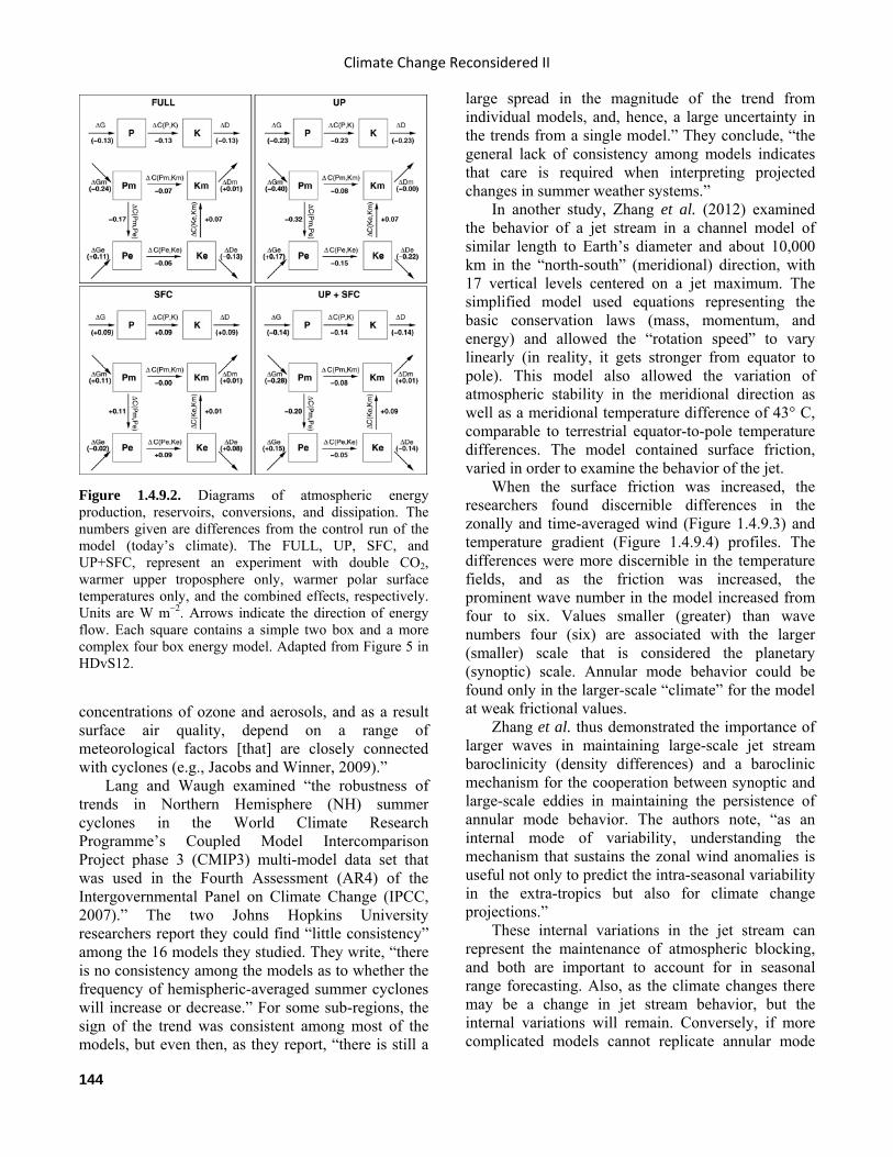
Climate Change Reconsidered II
144
concentrations of ozone and aerosols, and as a result surface air quality, depend on a range of meteorological factors [that] are closely connected with cyclones (e.g., Jacobs and Winner, 2009).”
Lang and Waugh examined “the robustness of trends in Northern Hemisphere (NH) summer cyclones in the World Climate Research Programme’s Coupled Model Intercomparison Project phase 3 (CMIP3) multi-model data set that was used in the Fourth Assessment (AR4) of the Intergovernmental Panel on Climate Change (IPCC, 2007).” The two Johns Hopkins University researchers report they could find “little consistency” among the 16 models they studied. They write, “there is no consistency among the models as to whether the frequency of hemispheric-averaged summer cyclones will increase or decrease.” For some sub-regions, the sign of the trend was consistent among most of the models, but even then, as they report, “there is still a
large spread in the magnitude of the trend from individual models, and, hence, a large uncertainty in the trends from a single model.” They conclude, “the general lack of consistency among models indicates that care is required when interpreting projected changes in summer weather systems.”
In another study, Zhang et al. (2012) examined the behavior of a jet stream in a channel model of similar length to Earth’s diameter and about 10,000 km in the “north-south” (meridional) direction, with 17 vertical levels centered on a jet maximum. The simplified model used equations representing the basic conservation laws (mass, momentum, and energy) and allowed the “rotation speed” to vary linearly (in reality, it gets stronger from equator to pole). This model also allowed the variation of atmospheric stability in the meridional direction as well as a meridional temperature difference of 43° C, comparable to terrestrial equator-to-pole temperature differences. The model contained surface friction, varied in order to examine the behavior of the jet.
When the surface friction was increased, the researchers found discernible differences in the zonally and time-averaged wind (Figure 1.4.9.3) and temperature gradient (Figure 1.4.9.4) profiles. The differences were more discernible in the temperature fields, and as the friction was increased, the prominent wave number in the model increased from four to six. Values smaller (greater) than wave numbers four (six) are associated with the larger (smaller) scale that is considered the planetary (synoptic) scale. Annular mode behavior could be found only in the larger-scale “climate” for the model at weak frictional values.
Zhang et al. thus demonstrated the importance of larger waves in maintaining large-scale jet stream baroclinicity (density differences) and a baroclinic mechanism for the cooperation between synoptic and large-scale eddies in maintaining the persistence of annular mode behavior. The authors note, “as an internal mode of variability, understanding the mechanism that sustains the zonal wind anomalies is useful not only to predict the intra-seasonal variability in the extra-tropics but also for climate change projections.”
These internal variations in the jet stream can represent the maintenance of atmospheric blocking, and both are important to account for in seasonal range forecasting. Also, as the climate changes there may be a change in jet stream behavior, but the internal variations will remain. Conversely, if more complicated models cannot replicate annular mode
Figure 1.4.9.2. Diagrams of atmospheric energy production, reservoirs, conversions, and dissipation. The numbers given are differences from the control run of the model (today’s climate). The FULL, UP, SFC, and UP+SFC, represent an experiment with double CO2, warmer upper troposphere only, warmer polar surface temperatures only, and the combined effects, respectively. Units are W m−2. Arrows indicate the direction of energy flow. Each square contains a simple two box and a more complex four box energy model. Adapted from Figure 5 in HDvS12.
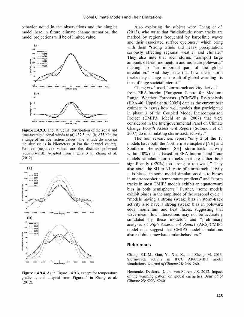
Global Climate Models and Their Limitations
145
behavior noted in the observations and the simpler model here in future climate change scenarios, the model projections will be of limited value.
Also exploring the subject were Chang et al. (2013), who write that “midlatitude storm tracks are marked by regions frequented by baroclinic waves and their associated surface cyclones,” which bring with them “strong winds and heavy precipitation, seriously affecting regional weather and climate.” They also note that such storms “transport large amounts of heat, momentum and moisture poleward,” making up “an important part of the global circulation.” And they state that how these storm tracks may change as a result of global warming “is thus of huge societal interest.”
Chang et al. used “storm-track activity derived from ERA-Interim [European Centre for Medium-Range Weather Forecasts (ECMWF) Re-Analysis (ERA-40; Uppala et al. 2005)] data as the current best estimate to assess how well models that participated in phase 3 of the Coupled Model Intercomparison Project (CMIP3; Meehl et al. 2007) that were considered in the Intergovernmental Panel on Climate Change Fourth Assessment Report (Solomon et al. 2007) do in simulating storm-track activity.”
The four researchers report “only 2 of the 17 models have both the Northern Hemisphere [NH] and Southern Hemisphere [SH] storm-track activity within 10% of that based on ERA-Interim” and “four models simulate storm tracks that are either both significantly (>20%) too strong or too weak.” They also note “the SH to NH ratio of storm-track activity ... is biased in some model simulations due to biases in midtropospheric temperature gradients” and “storm tracks in most CMIP3 models exhibit an equatorward bias in both hemispheres.” Further, “some models exhibit biases in the amplitude of the seasonal cycle”; “models having a strong (weak) bias in storm-track activity also have a strong (weak) bias in poleward eddy momentum and heat fluxes, suggesting that wave-mean flow interactions may not be accurately simulated by these models”; and “preliminary analyses of Fifth Assessment Report (AR5)/CMIP5 model data suggest that CMIP5 model simulations also exhibit somewhat similar behaviors.” References Chang, E.K.M., Guo, Y., Xia, X., and Zheng, M. 2013. Storm-track activity in IPCC AR4/CMIP3 model simulations. Journal of Climate 26: 246–260.
Hernandez-Deckers, D. and von Storch, J.S. 2012. Impact of the warming pattern on global energetics. Journal of Climate 25: 5223–5240.
Figure 1.4.9.3. The latitudinal distribution of the zonal and time-averaged zonal winds at (a) 437.5 and (b) 875 hPa for a range of surface friction values. The latitude distance on the abscissa is in kilometers (0 km the channel center). Positive (negative) values are the distance poleward (equatorward). Adapted from Figure 3 in Zhang et al. (2012).
Figure 1.4.9.4. As in Figure 1.4.9.3, except for temperature gradients, and adapted from Figure 4 in Zhang et al. (2012).
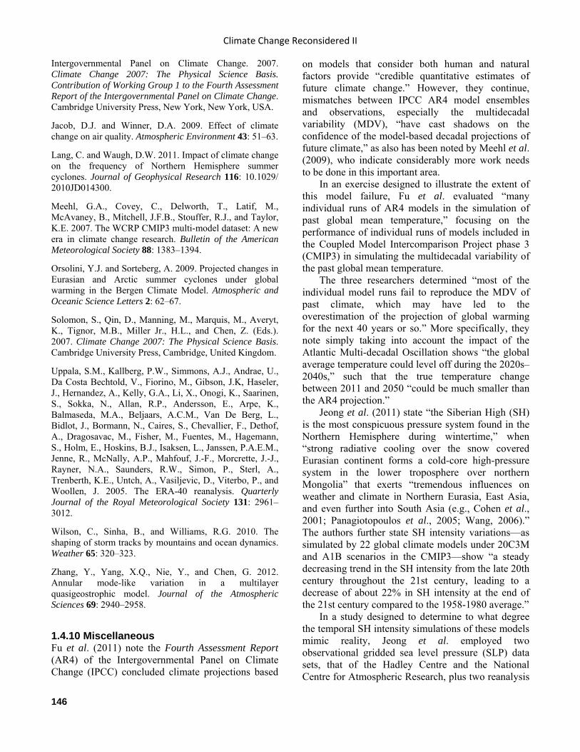
Climate Change Reconsidered II
146
Intergovernmental Panel on Climate Change. 2007. Climate Change 2007: The Physical Science Basis. Contribution of Working Group 1 to the Fourth Assessment Report of the Intergovernmental Panel on Climate Change. Cambridge University Press, New York, New York, USA.
Jacob, D.J. and Winner, D.A. 2009. Effect of climate change on air quality. Atmospheric Environment 43: 51–63.
Lang, C. and Waugh, D.W. 2011. Impact of climate change on the frequency of Northern Hemisphere summer cyclones. Journal of Geophysical Research 116: 10.1029/ 2010JD014300.
Meehl, G.A., Covey, C., Delworth, T., Latif, M., McAvaney, B., Mitchell, J.F.B., Stouffer, R.J., and Taylor, K.E. 2007. The WCRP CMIP3 multi-model dataset: A new era in climate change research. Bulletin of the American Meteorological Society 88: 1383–1394.
Orsolini, Y.J. and Sorteberg, A. 2009. Projected changes in Eurasian and Arctic summer cyclones under global warming in the Bergen Climate Model. Atmospheric and Oceanic Science Letters 2: 62–67.
Solomon, S., Qin, D., Manning, M., Marquis, M., Averyt, K., Tignor, M.B., Miller Jr., H.L., and Chen, Z. (Eds.). 2007. Climate Change 2007: The Physical Science Basis. Cambridge University Press, Cambridge, United Kingdom.
Uppala, S.M., Kallberg, P.W., Simmons, A.J., Andrae, U., Da Costa Bechtold, V., Fiorino, M., Gibson, J.K, Haseler, J., Hernandez, A., Kelly, G.A., Li, X., Onogi, K., Saarinen, S., Sokka, N., Allan, R.P., Andersson, E., Arpe, K., Balmaseda, M.A., Beljaars, A.C.M., Van De Berg, L., Bidlot, J., Bormann, N., Caires, S., Chevallier, F., Dethof, A., Dragosavac, M., Fisher, M., Fuentes, M., Hagemann, S., Holm, E., Hoskins, B.J., Isaksen, L., Janssen, P.A.E.M., Jenne, R., McNally, A.P., Mahfouf, J.-F., Morcrette, J.-J., Rayner, N.A., Saunders, R.W., Simon, P., Sterl, A., Trenberth, K.E., Untch, A., Vasiljevic, D., Viterbo, P., and Woollen, J. 2005. The ERA-40 reanalysis. Quarterly Journal of the Royal Meteorological Society 131: 2961–3012.
Wilson, C., Sinha, B., and Williams, R.G. 2010. The shaping of storm tracks by mountains and ocean dynamics. Weather 65: 320–323.
Zhang, Y., Yang, X.Q., Nie, Y., and Chen, G. 2012. Annular mode-like variation in a multilayer quasigeostrophic model. Journal of the Atmospheric Sciences 69: 2940–2958.
1.4.10 Miscellaneous Fu et al. (2011) note the Fourth Assessment Report (AR4) of the Intergovernmental Panel on Climate Change (IPCC) concluded climate projections based
on models that consider both human and natural factors provide “credible quantitative estimates of future climate change.” However, they continue, mismatches between IPCC AR4 model ensembles and observations, especially the multidecadal variability (MDV), “have cast shadows on the confidence of the model-based decadal projections of future climate,” as also has been noted by Meehl et al. (2009), who indicate considerably more work needs to be done in this important area.
In an exercise designed to illustrate the extent of this model failure, Fu et al. evaluated “many individual runs of AR4 models in the simulation of past global mean temperature,” focusing on the performance of individual runs of models included in the Coupled Model Intercomparison Project phase 3 (CMIP3) in simulating the multidecadal variability of the past global mean temperature.
The three researchers determined “most of the individual model runs fail to reproduce the MDV of past climate, which may have led to the overestimation of the projection of global warming for the next 40 years or so.” More specifically, they note simply taking into account the impact of the Atlantic Multi-decadal Oscillation shows “the global average temperature could level off during the 2020s–2040s,” such that the true temperature change between 2011 and 2050 “could be much smaller than the AR4 projection.”
Jeong et al. (2011) state “the Siberian High (SH) is the most conspicuous pressure system found in the Northern Hemisphere during wintertime,” when “strong radiative cooling over the snow covered Eurasian continent forms a cold-core high-pressure system in the lower troposphere over northern Mongolia” that exerts “tremendous influences on weather and climate in Northern Eurasia, East Asia, and even further into South Asia (e.g., Cohen et al., 2001; Panagiotopoulos et al., 2005; Wang, 2006).” The authors further state SH intensity variations—as simulated by 22 global climate models under 20C3M and A1B scenarios in the CMIP3—show “a steady decreasing trend in the SH intensity from the late 20th century throughout the 21st century, leading to a decrease of about 22% in SH intensity at the end of the 21st century compared to the 1958-1980 average.”
In a study designed to determine to what degree the temporal SH intensity simulations of these models mimic reality, Jeong et al. employed two observational gridded sea level pressure (SLP) data sets, that of the Hadley Centre and the National Centre for Atmospheric Research, plus two reanalysis
Global Climate Models and Their Limitations
147
data sets (NCEP and ERA40) and in situ SLP observations from 20 stations located in the central SH region to create a history of SH intensity over the past several decades.
The climatic reconstructive work of the seven scientists revealed “a pronounced declining trend of the SH intensity from the late 1960s to the early 1990s,” which would appear to mesh well with GCM simulations presented in the IPCC AR4 that indicate a “steady weakening of the SH intensity for the entire 21st century.” The authors report, however, that in the real world the declining SH intensity trend “was sharply replaced by a fast recovery over the last two decades.” The thus note “this feature has not been successfully captured by the GCM simulations used for the IPCC AR4,” all of which predict “a steady decreasing trend in the SH intensity from the late 20th century throughout the 21st century.”
Jeong et al. conclude, “an improvement in predicting the future climate change in regional scale is desirable.”
References Cohen, J., Saito, K., and Entekhabi, D. 2001. The role of the Siberian High in Northern Hemisphere climate variability. Geophysical Research Letters 28: 299–302.
Fu, C.-B., Qian, C., and Wu, Z.-H. 2011. Projection of global mean surface air temperature changes in next 40 years: Uncertainties of climate models and an alternative approach. Science China Earth Sciences 54: 1400–1406.
Jeong, J.-H., Ou, T., Linderholm, H.W., Kim, B.-M., Kim, S.-J., Kug, J.-S., and Chen, D. 2011. Recent recovery of the Siberian High intensity. Journal of Geophysical Research 116: 10.1029/2011JD015904.
Meehl, G.A., Goddard, L., Murphy, J., Stouffer, R.J., Boer, G., Danabasoglu, G., Dixon, K., Giorgetta, M.A., Greene, A.M., Hawkins, E., Hegerl, G., Karoly, D., Keenlyside, N., Kimoto, M., Kirtman, B., Navarra, A., Pulwarty, R.S., Smith, D., Stammer, D., and Stockdale, T. 2009. Decadal prediction: Can it be skillful? Bulletin of the American Meteorological Society 90: 1467–1485.
Panagiotopoulos, F., Shahgedanova, M., Hannachi, A., and Stephenson, D.B. 2005. Observed trends and teleconnections of the Siberian High: A recently declining center of action. Journal of Climate 18: 1411–1422.
Wang, B. 2006. The Asian Monsoon. Springer, Berlin, Germany.