Giovanni De Micheli

Technical Report No. CSL- TR-92-551

November 1992

This research was sponsored by NSF and DEC under a PYI award

ffiGH LEVEL SYNTHESIS OF DIGITAL CIRCUITS

Giovanni De Micheli

Technical Report: CSL-TR-92-SS1

November 1992

Computer Systems LaboratoryDepartments of Electrical Engineering and Computer Sdence

Stanford UniversityStanford, CA 94305-4055

Abstract

This tutorial surveys the state of the art in high-level synthesis of digital drcuits.It will be published in Advances in Computers, Volume 35, edited by M. Yovits.

Keywords and Phrases: high-level synthesis, scheduling, binding, datath andcontrol synthesis.

Copyright @ 1992

by

Giovanni De Micheli

Contents11 Introduction.

2

23

2 Circuit modeling.2.1 Modeling languages.2.2 Absttact mO<kls. . .

7899

11

3 Compilatk»n and behavioral optimizatk»n.3.1 Compilation tochniques. . . . . . . . . . . .3.2 Optimization tochniques.. . . . . . . . . . .

3.2.1 Data-flow based b'ansfonnations. . .3.2.2 Conb'Ol-flow 00sed transf<X'ffiations. .

12131414IS1618

4 Structural syntbes~4.1 The design ~e. 4.2 Resources and consb'aints. .

4.2.1 Resources 4.2.2 Consb'aints. .. . .

4.3 Scheduling and binding. . .4.4 Estimation

20202122242627303233333435

5 Scheduling.5.1 Scheduling without resource consb'aints. 5.1.1 The ASAP and ALAP scheduling algmthms. ..

5.1.2 Scheduling under reJative timing constraints. . . .5.1.3 ReJative scheduling. . . . . . . . . . . . . . . . .

5.2 Scheduling with resource constraints. . . . . . . . . . . .5.2.1 The Integer Linear Programming model. . . . . .

5.2.2 List scheduling. 5.2.3 Other heuristic scheduling algorithms. 5.3 Scheduling algorithms for extended sequencing models. .

5.3.1 Scheduling and o~ration chaining. . . . . . . . .5.3.2 Hierarchical scheduling. . . . . . . . . . . . . . .5.3.3 Scheduling graphs with alternative ~ths. . . . . .

36373839

41

43

6 Data-patb synthesis and optimization.

6.1 Sharingandbinding 6.2 Resowce sharing in non-hierarchical sequencing graphs. . . .

6.3 Resowce sharing in hierarchical sequencing graphs. 6.4 Registersharing 6.5 Od1er binding and sharing problems. ... . . . . . . . . . .

iii

4344

4547

7 Control synthesw.7.1 Cootrol synthesis for non-hierarchical seqooncing graphs. 7.2 Control synthesis for hierarchical sequencing graphs. . . . . . . . .

7.3 Control synthesis for unbounded-latency sequencing graphs. . . . .

484950

8 Synthesis or pipelined circuits.8.1 Scheduling pipelined circuits. . . . . . . . . . . . .8.2 Resource sharing and binding for pipelined circuits.

51515252

9 High-level synthesis systems.9.1 The System Architect's Workbench. . . .9.2 The Olympus Synthesis System. . . . . .9.3 The Cathedral Synthesis Systems. . . . .

S410 Conclusions.

5411 Acknowledgements

iv

1 Introduction.

As digital hardware systems ~<Xne larger and more complex, engin~rs need even mae JX>werful design 1001 !i.Synthesis systems have been shown effective in providing an automaled way, or a computer-assiste<1 environment.

for integrated circuit design.Several advantages stem from using synthesis IOOls. starting from rehavioral circuit models. First, high-level

modeling languages allow designers to conceptualize circuits in a self-documenting fonn. that can be fairly indc.pendent of the target technology and design style. This JH'Ovides design portability and supJX>rl for incremenlalchanges in later design revisions. At the same time, it makes circuit design available to a larger ba.~ or enginccr!i.who master system design issues without reing expert in specific circuit technologies.

The second advantage provided by synthesis tools is correctness and optimality. While design correctness i~relying in part on the software implementation of algaithrns, and therefore hard to claim, it is obvious that thcreliability in handling large scale designs is higher when performed by automated means than when done by humanbeings. Design optimization at various levels is coupled to synthesis. High-level optimization is extremely crilil';11in achieving the best circuit implementation. because it affects the macroscopic circuit parameters.

Eventually, synthesis tools provide a shonening of design time, reducing both the design cost antI the time 10market Both factas are crucial in the competitive marketplace of integrated circuits.

Computer-aided synthesis of digital circuit has been introduced gradually over the last two decades. At fir!ilphysical design IOOls. and later logic synthesis and optimization JX'Ograms, became common in the design now 01"integrated circuits. Recently, high-level synthesis techniques have been proposed and used for research as well a~for some product-level design. While these techniques are not yet used ubiquitously, it is likely thatlhey will hav('positive impiM::t on digital design methodology.

High-~\lel synthesis is a broad term to define circuit synthesis from models that are more abstrctCt and gencrulthan logic ones. The circuit modeling problem is strongly related to high-level synthesis. because it defines th,'boundary of this domain. High-level modeling is done by means of Hardware Description LanguaRc.\" (HDLs), .,~mentioned in Section 2.1. The lack of standardization of HDLs suitable for synthesis has been a majc>r impedimentin the diffusion of high-level synthesis. We shall consider in Section 2.2 modeling issues with ~rticular rererencc 10abstract circuit models. based on graphs, that can serve as common basis for synthesis and that dcCf)uplc !iynthc!iisand optimization from the particular features of any given language.

High-le\lel optimization is coupled to synthesis. It is customary to gather optimization techniques into twoclasses. The former groups lIK>se optimizations that are independent on the circuit structure and that parullcl Ih,'techniques used in software optimizing compilers. Such techniques are described in Section 3.

The latter class consists of the algorithms fa creating and optimizing the data-path and the control-unit. Dal;.l-path synthesis consists of binding the operations of the data-flow model to time slots and to computational unit!i.The time-binding is often called scheduling of the operations. The physical binding is often called re,\"{)urce bindin,lland it may involve resource sharing. Control synthesis corresponds to interpreting the control-f1ow or the model ant!in constructing a control unit that activates the resources at the appropriate time and with the awropriate inputs ant!

destinations. Scheduling, resource binding and control synthesis are described in Sections 5, 6 and 7 respectively"Structural synthesis and the related tasks are described first as applied to non-pipelined circuits. ftlr the ~,k,~ (11'simplicity. Extensions to pipelined models are reported in Section 8.

We conclude this chapter by giving a shoo history of high-level synthesis and by describing and comparinghigh-level synthesis systems in Section 9. This review will give the reader an idea aboutthc state of Ihc. art in Ihl'

field, the success achieved by high-level synthesis and the present difficulties.

Circuit modeling.2

Circuit modeling plays a fundamental role in defining the synthesis task as well as in capturing essential features ora design. We consider in the sequel circuit models at both the functional and logic abstraction levels with behavioraland Slruclural flavors. At the former level, a circuit behavior can be captured by a set of lasks and a parlial orderon the set of tasks. The tasks may be general in nature, involving arithmetic or logic functions. Similarly, a circuitstructure can be described by a partition into functional units and their interconnection. At the logic level, a circuitbehavior can be modeled in terms of slales and lransilions. A circuit structure can be stated in terms of logic gale.'and their interconnection. Circuit behavior at the functional level, called soortly circuil behavior, is the slaring poinl

for high-level synthesis.Hierarchical models are oflen used to simplify the representation. The hierarchy can be used to rcn<lcr a m()(k'i

modular, by encapsulating some of its portions, as well as making possible the multiple usage of a (slIb)-modcl hymeans of a model call. The use of hierarchical models has been used exlensively in software (e.g. slIhroutincs).

Modeling languages.2.1

Hardware Description Languages are often used to represent the circuit behavior or itS structure, Modem HDLs.such as VHDL [37], Verilog [53] and VDL/I [25], support both a behavioral and a structural m()(lcling slylc. W('

will consider the former only, because high-level synthesis is not required for sb"Uctural models.A natural question to ask is why standard programming languages, like C, canoot be used to mcxlel hardwarr

behavicx. They can indeed, but in a restricted domain. Functional models of processors can re defined as ('programs, compiled and executed for validating the correctness. It is questionable though how useflll they can Ix'

for synthesis.There are several differences between standard programming languages and modem HDLs. Thc major oncs

stem from the foct that hardware circuitS can always provide JYdfallel streams of execution and that Lhe precisrtiming of the execution of the operations may be very important in hardware, HDLs have explicit definition of If()ports and provide some specification means for determining when some operations are executed and hy which Iinil.On the other hand, HDLs do not support complex memory reference mechanisms like pointers and structures.

Whereas the syntax of HDLs varies widely, most of Lhem are procedural, with an imperative semantics. Thcrcrort'Lhe designer models a set of tasks by sequencing assignmentS to variables by means of control-now cOIlstruc'L'i, such

as branching, iteration and model call.Digital circuitS perform Boolean operations and their semantics is the same in hardware and in soflwart.'.

Similarly, the semantics of the HDL control-flow constructS parallels that of common programming languagc.~. Tht'interesting differences between HDL and programming language semantics are related to the data lyres and lO lhl'

timing of the opera~ons,The fundamental data-type in HDLs is the Boolcan variable, When considering languages with impcrativ('

semantics, variables may store information. They may be assigned multiple values, and they rewin Ihe last valliruntil the next assignment occurs. Therefore a hardware mechanism has to be associated with the Sk)rnge, unless Ihrinformation of a variable is readily consumed. In this case, variables correspond to wires in the cirCllil. Otl1crwisc.

2

they relate to more complex structures, such as registers (with possibly multiplexed inputs and enables). This side-

effect. i.e. modeling implicitly storage in imperative HDLs, is not a desirable feature, and complicates synthesis.Other variables, often called meta-variables, can be used to simplify the representation. For example, mew-

variables can be integers that address elements of a vector. Iteration on meta-variables is permitLc<1. NoLe thai

meta-variables do not have a hardware counterpart, and they are expanded in an early synthesis swge.The timing semantics of HDLs is currently subject of wide discussion. Some HDLs, like VHDL and Verilog,

were conceived for circuit specification and simulation. Therefore their consb'ucts are geared toward the efficientsup}X>ft of event-driven simulation. Some constructs do not even have a hardware correspondence. Models in

VHDL and Verilog specify circuit behavior as a set of sequential statements. Since the languages do nol s)X';Cify iItiming semantics, synthesis policies are used to interpret the timing behavior. This has the unfortunate side-cffect oflinking the semantics of hardware models to a }X>licy and hence to a synthesis tool, at the expense or il~ generality.Conversely, the UDl.JI language as a formal hardware semantics, The timing of the operations in a UDL/I modelis linked to the states of an automaton, hence prescribing one execution interval for each operation. Preci!;enrs~is achieved at the expense of sacrificing some degrees of freedom in interpreting the model and in lowering till'

overall absttaction level.

Abstract models.2.2AbSb"act models capture the essential features of behavioral models, and decouple them from the langlJage. Behav-ioral models at the functional level of absb'aCtion are specified in terms of tasks and their dependencie,\'. A task isoften called an operation. For the sake of generality we assume thaltasks can be also No-Operations (NOPs). i.('.

fake operations that execute instantaneously with no side effect and that can be used as placeholdcrs. [)cJx:ndencil~sarise from several reasons. First, availability of data. When an input to an operation is the result or aoolher onl',then the former operation depends on the latter. SecolKl, serialization constraints. A task may have to rollow .1

second one regardless of data-dependency. A simple example is provided by the two following operations: loa<tingdata on a bus and raising a flag. The circuit model may require that the flag is raised after the data is I()aded. Third.dependencies may arise because two tasks share the same resource, that can service only one task al a time. Thusone task has to perform before the other. Note though that in general dependencies due to resource !iharing are nolpart of the original circuit specification, because the way in which resources are exploited is relu!c{! In lhl' rirl'llll

implementation.Many different models have been proposed to model the circuit behavior in terms of gr;dphs. We considc.r ill

this chapter only one model, called sequencing graph, that is a hierarchical combination of data-Jlo~v graphs. Thl'data-flow graph entities model the data-flow while the hierarchical linkage of the entities models the control now.

Let us consider first a flat sequencing graph, i.e. a data-flow mcxlel. It represents operations and data dependen-cies. It is a directed graph G(V, E) whose vertex set V = {Vi; i = 1,2, . .. ,nap.} is in one to one correspondcnl'l'

with the set of tasks. The directed edge set E = {('vi,vj);i,j = 1.2,...,nop.} is in correspondence with lhctransfer of data from an operation to another one. Data-flow graphs are acyclic and can be made polar by addingtwo vertices, called source and sink, that represent first and last tasks. They correspond to No-Operations and arc

labeled by Vo and VN respectively. Therefore the graph has nap. + 2 vertices and subscript N is inlerchangeab'l~with nap. + 1. Appropriate edges are added to link the source and sink to the other vertices. We say that vcrtcxVi is a predecessor (or immediate predecessor) of Vj when there is a path (or an edge) with tail I'; and head I).Similarly, we say that vertex Vi is a successor (or immediate successor) of Vj when there is a path (or iID edge) wi!h

3

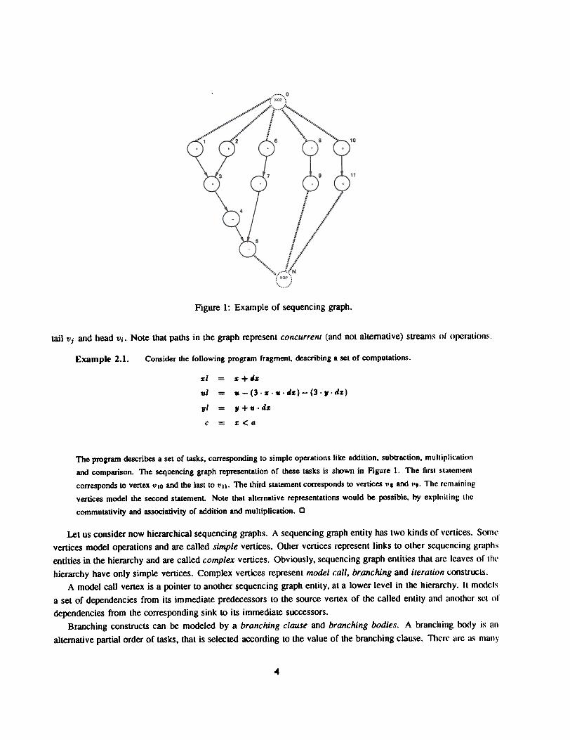
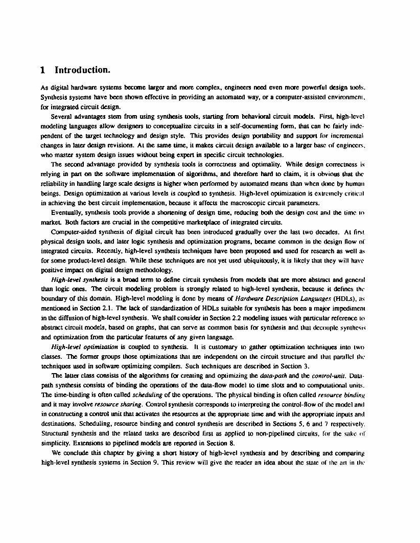
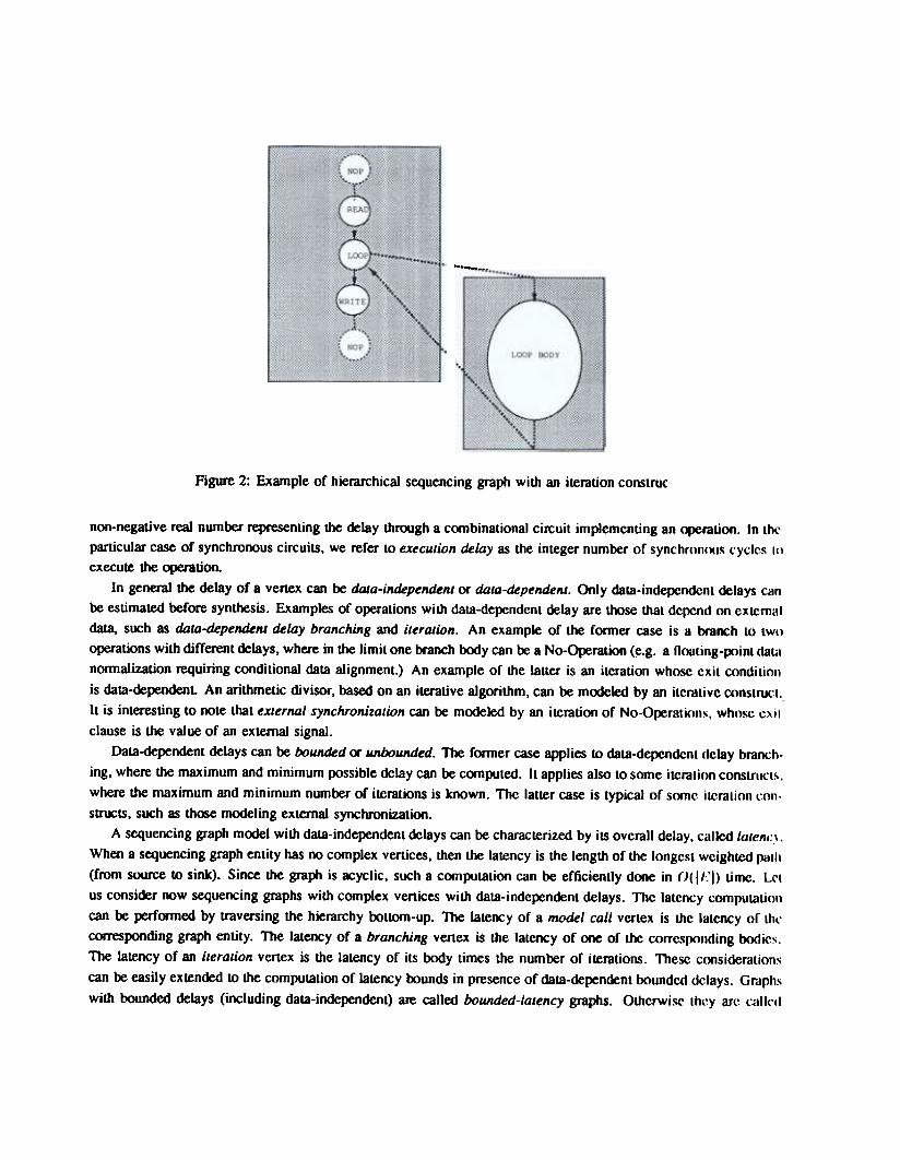
Figure 1: Example of sequencing graph.

tail Vj and head Vi. Note that paths in the graph represent concurrent (and not alternative) stream~ or opcralion!;

Consider the following program fragment, describing a set of computations.Example 2.1.

xl = x + dx

ul = u-(3.s...ds)-(3.,.dx)

1/1 = ,+ . . dxc = x<a

The program describes a set of tasks, corresponding to simple operations like addition, subtraction, multiplicalion

and comparison. The sequencing graph representation of these tasks is soown in Figure 1. The firSI ~tatcment

corresponds to vertex tllO and the last to t'll. The third statement corresponds to vertices t'l and '1'9. The remaining

vertices model the second statement. Note that alternative representations would be possible, by exploiling the

commutativity and associativity of addition and multiplication. 0

Let us consider now hierarchical sequencing graphs. A sequencing graph entity has two kinds of vcrtices. Soml'vertices model operations and are called simple vertices. Other vertices represent links LO other sequencing gruphsentities in the hierarchy and are called complex vertices, Obviously, sequencing graph entities that arc lcavcs of thl'

hierarchy have only simple vertices. Complex vertices represent model call, branching and iteration constrUCL'i.A model call vertex is a pointer LO another sequencing graph entity, at a lower level in the hierarchy. IL models

a set of dependencies from its immediaLe predecessors LO the source vertex of the called entiLy and ;Inothl~r Sl'.t of

dependencies from the corresponding sink LO its immediate successors.Branching constructs can be modeled by a branching clause and branching bodies. A branching bo<ly j!; all

alternative partial order of tasks, that is selected according to the value of the branching clause. Th('r(' arc as mallY

4

branching bodies as the possible values of the branching clause. Branching is modeled by associating a sequencinggraph entity to each branch body and a complex vertex to the branching clause. The selection of a hranch b<xly is

then modeled as a selective model caJlLO the corresponding sequencing graph.Iterative constructs are modeled by an iteration clause and an iteration body. An iteration (or I()()p) body is a

partiaI order of tasks, that is repeated as long as the iterative clause is asserted. Iteration is modeled in sequcncinggraphs through the use of the hierarchy, thus preserving the acyclic nature of the graph. Iteration is rcprescnlCd as

a repealed model callLO the sequencing graph entity modeling the iteration body.

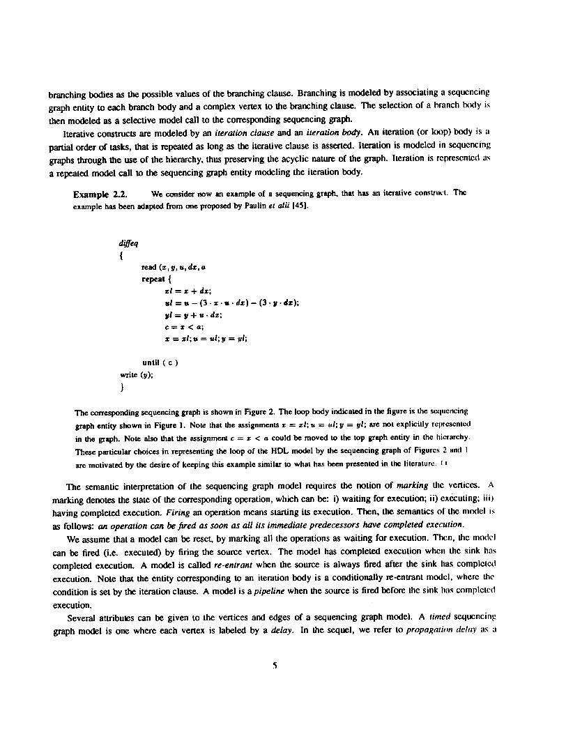
Example 2.2. We consider now an example of a sequencing graph. that has an iterative con~trllct. Thc

example has been adapted from one proposed by Paulin et alii [45].

diffeq{

read (X,l1,u,d%,a

repeat {sl = s + ds;ul = u - (3 . s . u . ds) - (3 . y . ds);

yl = y + u . ds;c = s < a;s = sl; u = ul; 11 = yl;

until ( c )

write (y);

}

The corresponding sequencing graph is shown in Figure 2. The loop tx>dy indicated in the figure is lhe sC<llIcncing

graph entity shown in Figure 1. Note lhat lhe assignments x = xl; 1~ = 1~1; Y = yl; are not explicitly rcprc.4;colcd

in lhe graph. Note also lhat lhe assignment c = x < a could be moved to the top graph entity in lhc hil.'farchy.

These particular choices in representing the loop of the HDL model by the sequencing graph of Figurc!' 2 and 1

are motivated by the desire of keeping lhis example similar to what has been presented in the lileraturc.~. [I

The semantic interpretation of the sequencing graph model requires the notion of marking tllC venices. A

marking denotes the state of the corresponding operation, which can be: i) waiting for execution; ii) executing; iii)having completed execution. Firing an operation means starting its execution. Then, the semantics of the mCKlel is

as follows: an operation can be fired as soon as all it.\" immediate predecessors have completed execution.We assume that a model can be reset, by marking all the operations as waiting for execution. Thcn, the m()(lel

can be fired (i.e. executed) by firing the source venex. The model has completed execution when the sink hascompleted execution. A model is called re-entrant when the source is always fired after the sink has complclc~1execution. Note that the entity corresponding to an iteration body is a conditionally re-entrant mO(lcl, where thecondition is set by the iteration clause. A model is a pipeline when the source is fired before the sink hilS complclell

execution.Several attributes can be given to the vertices and edges of a sequencing graph model. A timed scqucncinl,:

graph model is one where each venex is labeled by a delay. In the sequel, we refer to propop,otifln delay as .1

~

~

Figure 2: Example of hierarchical sequencing graph with an iteration construc

non-negative real number representing the delay through a combinational circuit implementing an operation. In thc

particular case of synchronous circuits, we refer to execution delay as the integer number of synchronOtI~ cycl('.~ III

execute the ~tion.

In general the delay of a vertex can be data-independent or data-dependent. Only data-indepcndcnt delays can

be estimated before synthesis. Examples of operations with data-dependent delay are those that depend on extern,,'

data. such as data-dependent delay branching and iteration. An example of the former case is a braoch to tWtl

operations with different oolays, where in the limit one branch body can re a No-Operation (~.g. a tloating-lX>int claUI

normalization requiring conditional data alignment.) An example of the laUer is an iteration whose exit conditioll

is data-oopendenL An arithmetic divisor, based on an iterative algorithm, can be m<xleled by an itcrdlive constrocl..

It is interesting to note that external synchronization can be modeled by an iteration of No-°lX'.r'dtiOtls, wh()Sc cxil

clause is the value of an external signal.

Data-dependent delays can be bounded <X" unbounded. The former case applies to data-dependcnt delay branch-

ing, where the maximum and minimum possible delay can be computed. It applies also to some iterati()n cOnstnICl where the maximum and minimum number of iterations is known. The latter case is typical of S()In(' ilcralion l:OI1.

strocts, such as those modeling external synchronization.

A sequencing graph model with data-independent delays can be characterized by its overall delay, callcd latenl:.}.

When a sequencing graph entity has no complex vertices, then the latency is the length of the longest weighted palh

(from source to sink). Since the graph is ~yclic, such a computation can be efficiently done in O( I 1-:1) time. Lcl

us consider now sequeocing graphs with complex vertices with data-independent delays. The latency computatioll

can be performed by traversing the hierarchy bottom-up. The lateocy of a model call vertex is the lalency of lhl'

corresponding graph entity. The latency of a branching vertex is the latency of one of the corresponding bodic~.

The latency of an iteration vertex is the latency of its body times the number of iterations. These considerations

can be easily extended to the computation of lateocy bounds in presence of data-dependent bounded delays. Grdphs

with bounded delays (including data-independent) are called bounded-latency graphs. Otherwise thl~y arc call(,11

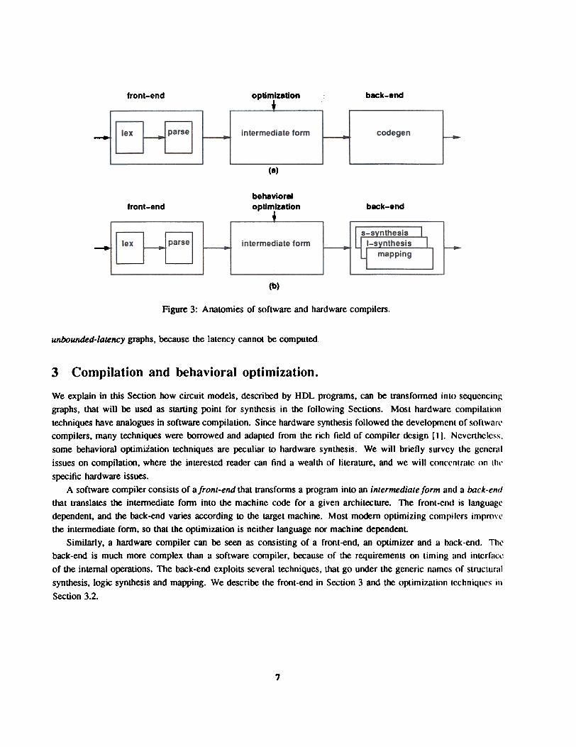
front-end optimization- - t .. back-end

intermediate form-(8)

front-end back-endbehavioraloptimization

. i .

intermediate form-..

(b)

Figure 3: Anatomies of software and hardware compilers.

unbounded-latency graphs, because the latency cannot be computed.

Compilation and behavioral optimization.3

We explain in this Section how circuit models, descrired by HDL programs, can be transfonned inLo sequencinggraphs, that will be used as starting poinL for synthesis in the following Se(:tions. Most hardware compilaLiontechniques have analogues in software compilation. Since hardware synthesis followed the developmenL of sofLwarl'compilers, many techniques were borrowed and adapLed from the rich field of compiler oosign [II. NeverLhcless.some behavioral optimization techniques are peculiar to hardware synLhesis. We will briefly survey the generalissues on compilation, where the interesLed reader can find a wealth of literature, and we will conccnlralc on Lhl'

specific hardware issues.A software compiler consists of afront-end that transfonns a program into an intermediate form and a back-end

that translates the intennediate fonn into the machine code for a given architecture. The fronL-en<l is languagcdependent, and the back-end varies according to the Larget machine. Most modem optimizing comrilc.rs imrm\'('the intennediate fonn, so that the optimization is neither language nor machine dependent

Similarly, a hardware compiler can be seen as consisting of a front-end, an optimizer and a back-end. Thcback-end is much more complex than a software compiler, because of the requirements on Liming and inlCrfacl~of the internal operations. The back-end exploits several techniques, that go under the generic names of strucluralsynthesis, logic synthesis and mapping. We describe Lhe front-end in Section 3 and the optimizalion Ic.chniqllcs ill

Section 3.2.

7

Compilation techniques.3.1

The front-end of a compiler is responsible for lexical and syntax analysis, parsing and creation of the intermediateform. A lexical analyzer is a component of a compiler that reads the source mcxiel and produces as an output a selof tokens that the ~er then uses for syntax analysis. A lexical analyzer may also ~rform ancillary la~ks, ~uch (IS

stripping commentS and expanding macros.A parser receives a set of tokens. ItS task is to verify first that they satisfy the syntax rules of me language.

The parser has knowledge of the grammar of the language and it generales a set of parse trees. A parse tree is atree-like representation of the syntactic structure of a language. Syntactic errors, as well as some semantic ent)r~

( such as an operator applied to an incompatible operand), are detected at this stage. The error recovery policydepends on the compiler and on the gravity of the ent)r. Software tools can be used to create lexical analyzers andparsers. The most commonly used ones are programs lex and yacc provided with the UN I ,yT M operating sysLCm.

While the front-end of a compiler for software and hardware are very similar, the subsequent sleps may tic rmrlydifferent. In particular, for hardware languages, diverse slrategies are used according to their flavors.

The compilation of hardware models at the functional level involves a full semantic analysi.\", lhat compri~c~data-flow and control-flow analysis and type checking. Semantic analysis is performed on the parse trcc-~ in difrercnlways. A common one is ftaltening the parse trees and creating me intermediate form. In doing this, me semanticsof the model is checked. Type checking has some peculiarity when compiling HDLs. Operations on vectors or

Boolean variables are checked for operand compatibility. Vectors may be padded with ones or zen~~ 10 a(~hirvl'

compatibility in some cases.The overloading of the arithmetic and relational operators has to be resolved at this stage. First, all metavariables

need to be eliminated, by expanding the constructS lhal employ them, because metavariables have no correspondinghardware semantics. The operators on integer metavariables (both arithmetic and relational) have mc usual meaning.By contrast, operations on Boolean vectors have to be mapped to hardware o~rators that do the correspondingfunction. For example, the sum of two Boolean vectors has to be resolved as a link to an adder circuit. Similarly.the comparison of two integers, to be implemented in hardware by Boolean vectors, has to be mapped lo a link

to a hardware comparator. Since the mapping to hardware resources is not always univalent, (becuuse differel1lhardware implementations have different area/performance parameters) abstract hardware operators ure used allhisstage and the binding to hardware resources is deferred to a later oplimi-z.ation stage (described in Section 6.)

The semantic analysis of the parse trees leads to the creation of the intermediate form, lhat rcpresenl~ L!'"'implementation of the original HDL program on an abstract machine. Such a machine is identified by a sel oroperations and dependencies, and it can be represenLCd graphically by a sequencing graph. The hardware modelin terms of an abstract machine is virtual in the sense that it does not distinguish the area and delay costs of throperations. Therefore, behavioral optimization can be performed on such a model while abstracting Ihe un<k'rlyin,!!

circuit technological parameters.We assume here, for the sake of explanation and uniformity, that the sequencing graph mo<lel is used as

intermediate form. Note that other intermediate models could be used, with similar meaning but dirfcrem a.~J}C('ls.Similarly we assume here, for the sake of simplicity, that structured programming constructS are used (e.g. rn)unrestricted goto statementS are employed), and that each model has a single entry and a single exit points. n,isallows us to interpret the hardware model as a sequencing graph that abides the definition given in Section 2.2.

Whereas the hierarchical structure of the sequencing graphs is derived from the control-flow analysi.\" of lhcmodel, the graph topology is based on data-jiow analysis. The parse LrCCS for each assignmcnl ~Ullcmenl ~orr('-

R

spond then to the vertices of each graph entity. The edges are inferred by considering data-flow and !\crialii'.ation

dependencies. Each sequencing graph entity corresponds to a basic block in compiler jargon.Data-flow analysis comprises several tasks, and it is used as a basis for behavioral optimization. It entails the

derivation of the variable life-times, i.e, the interval between their first definition (birth) and last reference (death).Note that sequencing graphs do not model explicitly the fact that variables need storage during their lifetimes.with a corresJX>nding cost in terms of circuit implementation. When considering hardware models Wilh imperativcsemantics, multiple assignments to variable may occur. Variables preserve their values until the nexl assignmcnl.For hardware synthesis, it is often convenient to rename instances of variables, so that each instance has a singleassignment and, of course, to resolve the references appropriately. A scheme for variable renaming is presented in

reference [30].

Optimization techniques.3.2

Behavioral optimization is a set of semantic-preserving Lransformations that minimize the amount or informationneeded to specify the partial order of tasks. No knowledge about the circuit implementation style is required allhisstage. Behavioral optimization can implemented in different ways. It can be applied directly to the lhe parse LrCCS.or during the generation of the intermediate form, or even on the intermediate form itself, according lo the dirfercnlcases. For the salce of explanation, we consider here these transformations as applied to sequences or SlAltcmenl'i.

Transformations for behavioral optimization of HDL models can be classified as data-now and conLrol-l1oworiented. The former group resembles most to the transformations applied in software compiler!;. They rely on

global data-flow analysis of the intermediate form.

Data-flow based transformations.3.2.1

These transformations are dealt with in detail in most books on software compiler design [1] and 1~41

Tree-height reduction. This transfonnation applies to the arithmetic expression trees, and strives lo achieve thl'best-possible expression split into two-operand expressions, so that the paral1elism available in hardware can b('exploited at best It can be seen as a local transfonnation, applied to each compound arithmetic Slatement, or asa global transformation, applied to all the compound arithmetic Slatemenls in a basic block. Enough hardwarl'resources are postulated to exploit all the parallelism. If this is not the case, the gain of applying thc. Lr.lnsformalio'l

is obviously reduced.

Example 3.1. Consider the following arithmetic assignment: x = a + b + c + d; that can be trivially !'plit a.~:

x = a + b; x = x + c; x = x + d;. It requires three additions in series. Alternatively, the following split can hc

done: p = a + b; q = c + d; x = p + q;, where the ftrst two additions can be done in parallel if enough rcsnurcc~

are available (in this case, two adders). The second choice is better than the first one, because the C()rrcsp')nding

implementation cannot be inferior, for any possible resource availability. 0

Constant and variable propagation. Constant propagation, also called constant folding, consislli of detectingconstant operands and precomputing the value of the operation with that operand. Since the result may be again ;t

constant. then the new constant can be'propagated to those operations that use it as input.

9

Example 3.2.. Consider the following fragment: A = 0; b = . + 1; c = 2. b;. It can be fCpI..-aI hy

a = 0; b = 1; c = 2;. 0

Variable ~atiOll, also called copy pro~gation, consists of ~ting the copies of variables, i.e. lh('assignments like .1.' = y, and using me righl-hand side in me following references in place of me Icrl-hand side.Dala-flow analysis permits lO identify lhe Slatements where lhe lransformalion can be done. In particular lhc"~gation of y C8I1JQ be done after a ditTerenl reassignmenllO z. Variable p-opag81ion gives lhe opJX>rtunilY lOremove men me copy assignment NOle Lhal copy assignments may have been inlrOdoced by olher lrulI~rormalions.

Example 3.3. Consider the following fragment: a = %; b = 11+1; c = 2. a;. It can be replM:OO bya := %; b = % + 1; c = 2. X;. Statement a = x; may then be removed by dead code elimination, ir Ihcrc ar~

no further references to a. 0

Common subexpression elimination. The search for common logic surexpressions is rest done by I()gic synthc~i~algorithms. The search for common arithmetic surexpressions relies in general on finding isomorphic pallCms inthe ~ trees. This step is greatJy simplified if the arithmetic expressions are redoced to two-inpul ones. TlX'cn.this b1mSfmnation consists of selecting a target arithmetic operation, and searching for a preceding one of the saml'type and with the same operands. OperatOr commutativity can 00 exploiled. Again, data-flow analy!;is is uscd inthe search, to insure that in any matching expression the operands always take the same values. When a precedingmatching exp-ession is found, then the larget expression is replaced by a copy of the variable lh:.ll j!; ll\C rC!ilJll nI'the preceding matching expression.

Example 3.4. Comider the following fragment: " = r + J; b = a + 1; c = x + If;. ]t C8n he repl8Coo

by: CI = x + If; b = CI + 1; c = a;. Note 1h8t a variable copy h..~ been introduced for variable fI, Ihlll can he

propag8led in the subsequent code. 0

Dead code elimination. Dead code consists of alllhose operations thal cannot be reached, or whose result is ncv('rreferenced elsewhere. Such operations are detecled by data-flow analysis and removed. Obvious cases are lJ'l(,st'statements that would follow a procedure return stalernent. Less obvious cases involve opcralions mal just prcc('{I,'a return statement and whose results arc not parnmelers of the procedure nor Uk:y affcct any of il'i l~'ram('ll'.rs.

Example J.5. Consider the following fragment: a = %; 6 = , + Ii C - 2. x;. If vaTiahlt" ., i!i ""Ireferenced in the sut.equent code, the first assignment can be removed. C

Operator strength reduction. Operator strength rOOuction means rOOucing !he cost of implemenling an ~ral()fby using a simpler one. Even though in principle some notion of the hardware implementalion is required, vcryoften general considerations apply. For example, a mulliplication by two (or by a power of lWO) CUll he rcpluc('(1by a shift. ShifleJ'S are always faster and smaller man multipliers in many implemenlauons.

Example 3.6. Comider the following fragment: a = %2

X «1; b = x + t;. 06=3..r It can be replaced by

10

Code motion. Code motion often applies to loop invariants, i.e. quantities that are computed inside an iterativeconstruct but whose values do not change from iteration to iteration. The goal is to avoid the repelilivc cvrnualion

of the same expression.

It can be b'ansfnrmoo to:Example 3.7. Consider the following iteration clause: for (i = l;i:5.. 6){t = a . b; for (i = 1; i :5 t){ }. 0

..

3.2.2 Control.ftow based transformations.

The following transformations are typical of hardware compilers. In some cases these transformations arc automate.d,

in others they are user-driven.

Model expansion. Writing structured models, by exploiting subroutines and functions, is useful for two mainreasons: modularity and re-usability. Modularity helps in highlighting a particular task (or set of ulsks). Often.

calls to a model are done only once in a HDL model.Model expansion consists in flattening locally the model call hierarchy. Therefore the called mooel disappears.

being swallowed by the calling one. A possible benefit is that the scope of some optimization techniques (at diffcrcntlevels) is enlarged, yielding possibly a better final circuit. If the expanded model was called only once, there is nonegative counterpart. Nevertheless, in the case of multiple calls, a full expansion leads to an increasr in the size or

the intermediate cooe and to the probable loss of the possibility of hardware sharing.

Example 3.8. Consider the following fragment: x = a + b; y = a * b; z = /oo(x..l/I; wherc:foo(p,q){t = q - p; return(t);}. Then by expanding too. we have: x = a + b; y = a * b; z = 1/ .."; 0

Conditional expansion. A conditional construct can be always b"ansformed into a parallel construcl with a te...t inthe end. Under some circumstances this transformation can increase the performance of the circuit. For example.this happens when the conditional clause depends on some late-arriving signals. Unfortunately this transformationprecludes some possibilities for hardware sharing, because the operations in all bodies of the branching construct

have to be performed.A special case applies to conditionals whose clauses and bodies are evaluation of logic functions. Then. thr

conditional expansion is favorable because it allows us to expand the scope of logic optimization.

Example 3.9. Consider die following fragment: y = ab; if (II) {x = b + d;} else {r = "";}. Theconditional statement can be flattened to: x = a(b + d) + a 'bd and by some logic manipulation. die fragment cltn

be rewritten as: y = ab; x = y + d(a + b). 0

Loop expansion. Loop expansion, or unrolling, applies to iteraLive COnSLruCLs with daLa-indepcndcnL exiL condi-tions. The loop is reploced by as many inSLances of iLs body as the number of operations. The bcncfiL is again inexpanding the scope of other transformations. Needlcss to say, when the number of iLeraLions is lilrgc. unrolling

may yield a large amount of code.

ThcExample 3.10. Consider the following fragment: :r = 0; for (i = 1;; ~ 3;i + +loop can be flattened to: x = 0; x = x + 1; x = x + 2; x = x + 3. 0

{%: = r + I;

Other ttansformations on loops are possible, such as moving the evaluation of the iterative clallsc from the top

to the bottom of the loop [54].

II

Block-level transformations. Branching and iterative constructs segment the intermediate cooe into basic blocks.Such blocks correspond to the sequencing graph entities. Trickey studied the possibility of manipulating thc sizcof the blocks, by means of block-level transformations, that include block merging and expansions or conditionalsand loops. Even though he did not consider model expansion, the extension is straightforward. Hc assumed thaioperations in different blocks cannot overlap execution and that concurrency is limited only by Ihe amrntnl or

hardware resources available for parallel execution in each block.Therefore, collapsing blocks may provide more parallelism and enhance the average performancc. To find

the optimum number of expansions to be performed, he proposed five transformations, with rules lo mcasure thcexpected performaJK:e improvement. The rules can then be applied bottom-up in the hierarchy indlK:ed by thccontrol-flow hierarchy of the model. He proposed a linear-time dynamic JX"ogramming algorithm, that returns anoptimum block-level structure. Unfortunately, the optimality is weakened by the assumptions on thc model and on

the transformation rules. We refer the interested reader to reference [541 for further details.

Structural synthesis.4

Structural synthesis is the creation of the macroscopic structure of a digital circuit. The starting point ror structuralsynthesis is a circuit behavioral view at the functional level, that can be fully captured by a sequencing graph. Thrresult of structural synthesis is a structural view, i.e. an interconnection of the major building blocks of a circuil.In other words, structural synthesis transforms a partial order of operations into an interconnection or operators .Irnl

a corresponding control circuit.Structural synthesis may be performed in many ways, according to the assumptions on the hardware being

designed, the design style and the design goals. Therefore a large variety of problems, algorithms and lO()ls hav\:been proposed, that fall under the umbrella of structural synthesis. To be more specific, we address in this Section

the synthesis problems for synchronous mono-phase digital hardware.Even by focusing the structural synthesis task to one particular implementation style, the spectrum of solutions

is still very wide. Indeed, the designer's goals in using a structural synthesis tool may be quite different. The m.tjor

ones are to preserve the specified behavior, while optimizing the performance or the area of the implementation.Some further clarifications are needed at this point. First, the area and performance can only be estimalCd at thisstage, because only the macroscopic structure of the circuit is dealt with. Second, worst case \)()l1nds on arc<1and on performance may be required. No matlCr how fast a chip runs, its yield may drop above a certain sizeand/or manufacturing may be unfeasible. Similarly, compact implementations that fall below a certain levc.1 orperformance may be irrelevant Third, the circuit structure may be constrained to using some prc-sllCcific<1 I1nil..

for some operations or to have auxiliary 1/0 or test circuits in appropriate positions.In general, the designer may be interested in exploring a set of trade-off points corresponding to area/pcrformanc('

estimates. The design space consists of all feasible stroctures that correspond to a given behavior. StruClur.11synthesis tools can be used to traverse the design space, by providing a designer with information about thcs<.'estimates. Alternatively, structural synthesis can compute one point of the design space corrcsl)I)nding to aI'

implementation that satisfies a particular optimality criterion.We partition structural synthesis into two tasks. The former is the search for an optimal structure in the. design

space. Optimality can be defined according to different criteria and possibly subject to constraints. The underlyingmodel is the sequencing graph model extended with annotations. The second task is to synthesize lhc (lat1t-path urnl

the control circuits corresponding to the chosen structure as interconnection of logic blocks.

12

A~ CJGl8~~

A~-.

ar-

~ '.- .

A;:- . I

~

.

.\ =6 ~. ! ~i CGJal_- - I

Lat.~~.

Lat._y(oyo1'-:~~ -. )

Lat-...

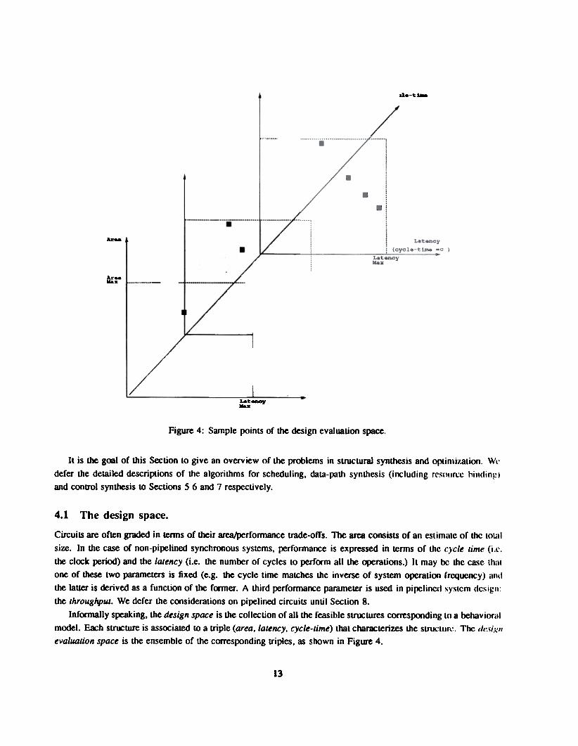
Fjgure 4: Sample points of the design evaluabon space.

It is the gool of this Section to give an overview of the problems in structural synthesis and optimi7.8tion. Wl'

defer the detailed descriptions of the algorithms for scheduling, data-path synthesis (including rCS()llrcc himling)

and conb"ol synthesis to Sections 5 6 and 7 respectively.

4.1 The design space.

CircuilS are often graded in lenDS of their area/perfonnance trade-offs. The area consists of an eslimalc or lhc [owl

size. In the case of non-pipelined synchronous systems, perrormance is expressed in lenDS or thc cycle time (i.t'.

the clock period) and the latency (i.c. the number or cycles lO perrorm all the ~rations.) Il may re thc ca.~c lh.11

one of these two parameters is fixed (e.g. the cycle lime matches the inverse of sYSlem operation rrequency) anti

the lalter is oorived as a function of the former. A third perfonnance parameter is used in pi~linC(1 ~y~lcm dc~igl1:

the throughput. We defer the considerations on pipelined circuilS until Section 8.

Infonnally speaking, the design space is the collection of all the feasible SlrOCtures conesponding lo a behaviorul

model. Eoch SlrOCture is associated 10 a lriple (area. latency. cycle-time) that chanM;terizes the SlruC[lIn~. Thc de.ti.I.'"

evaluation space is the ensemble or the corres)X>nding triples, as shown in Figure 4.

13

Realistic design examples have shown that the design evaluation space is not a smooth surface. This is dueto two reasons. First, the design space is a finite set of pointS, because the macroscopic structure of a circuit hasa coarse grain. For example, a hypothetical circuit may have one or two multipliers, and itS area would jump in

correspondence of this choice. Second, there are several non-linear effectS that are compounded in dctcrmining thc

area, latency and cycle-time as a function of the structure of the circuit.The goal of sb'Uctural optimization is to minimize one or more of the entries in the triple, under possibly somc

bounds on the remaining ones. Therefore, structural synthesis involves a constrained multi-criteria optimizationproblem. Due to the lack of compacUless of the design space and of smoothness of the design evaluation space, thc

solution methods are fairly involved and rely on a combination of techniques that solve some related sllb-prohlcms.

Resources and constraints.4.2Hardware behavior is described by the set of the operations, their relations and by the inner models of the operationsthemselves. The operations and their relations can be represented by a sequencing graph, that capturc.Ii Ihe operations

and their partial order.The operations are preformed in hardware by operators, called resources. Resource models are also required by

structural synthesis. It is important to remark that a circuit constructed by structural synthesis does not contain onlyresources. Indeed, it comprises also steering logic circuits, (e.g. multiplexers and busses), to send the data to tht:appropriate resources at the appropriate time, registers to hold data across cycle ooundaries, and control circuit.\' II)

sequence and synchronize the operations.Constraints are also an integral part of the hardware model. Timing constraints, such as operation serialii'.3tion

and bounds on the separation between two operations can be seen as part of the required behavior. They canbe described as additional relations added to the sequencing graph mcxlels. Other constraints, such as area orperformance bounds, can be seen as frontiers that delimit the design space. They are not part of the hardw~lre

behavior, but they are part of the hardware specifications.

4.2.1 Resources.

Hardware resources are the circuits that implement the operations. corresponding to the vertices. A liassificmiml

of the resources can be done according to the type of operations. Namely:

. Functional resources yield a result as a function of some input data. Examples are arithmetic opt.'.ral.or!i (c.g

adders, multipliers, ...), combinational and sequcntiallogic functions.

. Memory resources store data. Examples are registers, read-only and read-write memory arrays.

. Interface resources support internal communication (e.g. busses) and external inpul/outpliL lilnCli()n~. thai

allow the circuitLO communicate with the external environment

In addition, when considering hierarchical sequencing graph models, complex vertices may represenl calls lO othersequencing models. These models themselves, once synthesized in hardware, can re seen as crnnhinatiornll or

sequential logic functions and treated as functional resources.Functional resources represent the widest class of hardware operators. Indeed, there are as many kinds of

these resources as there are many ways of implementing operations in hardware. Most algorithms for strUCluraloptimization exploit different choices and combinations of functional resources in the traversal of lh(' (!('.sign SPCI('('.

14

Memory resources include registers and memory arrays, whose access can easily be modeled as Lransfer of cia\;)

across circuit P<X1S. Therefore an often used paradigm for memory resources is not to describe them cxplicilly in

the sequencing graph model but assume that their usage is implied by the behavioral model.Interface resources include busses, that may be used as a major means of communication inside a dala-~th.

External va resources are in general standard circuits, and access to them can also be modeled as Lr,lnsfcr of datil

across circuit P<X1S.

We say that a circuit is resource-dominated if the total area and delay depend mainly ulX>n thc area and delayof the resources. This is the case of most DSP circuits, that employ several standard resources, such as arithmcti(.~units. Conversely, the parameters of ASIC circuits depend often on control and on application.spec~/ic logic units.

SLrUclUral synthesis of resource-dominated circuits benefits from simpler estimation methods.

4.2.2 Constrain~.

Constraints in sb"Uctural synthesis can be classified inLo Lwo major groups: interface constraints and implementation

constraints. InLerface consLrainlS are part of the hardware behavior. To understand the reason for this, we must

view the circuiL interface as a parLition boundary belween the behavior and the environment. This parliLion forces

some implementation choices LO be dictated by the environment, such as the size and the timing of the data transfer.

The size of the data being transferred is related LO the number of I/O pins of the chip. It is a hardware C()fISlrainl

that is generally related to the size of the port variables of the model. The timing of Lhe data being lrdnsferrcd can

be specified by means of detailed timing constrainlS, that specify Lhe minimum and or maximum delay betWCCll

any pair of operations, and in particular I/O operaLions. Detailed Liming constraints are describc<1 in Scclion 5.1.2

as well as the algoriLhms LO validate their consistency and LO enforce Lhem.

Implementation constraints reflect the desire of the designer Lo achieve a Sb"Ucture with some properties. Ex-

amples are area consLraints and performance constraints, in terms of lhe cycle time (i.e. lhe clock pcricxl) and till'

latency (i.e. the number of cycles to perform all the operations.)

A different type of implementation constraints is the resource mapping constraint In Lhis ca.~c, a particular

operation is consn-ained to be implemenLed by a given resource. These constraints are motivaled by lhc designer's

previous knowledge, or inLuition, thaL one parLicular choice is the besL and thal other choices do DOL nce<1 invesLiga-

tion. Structural synthesis wiLh resource mapping constrainlS is often referred LO as synthesis from partial ,~truclun~

[26]. Design systems thal support such a fealure allow a designer lO specify a system in a wide spccLrum of ways.

ranging from a full behavioral model to a strucLural one. This modeling capabiliLy may be useful lO Icvcragl'

previously designed componenlS.A common overall goal in structural synthesis is LO maximize lite circuil performance (e.g. minimize laLcncy

and/or cycle-times) under area constraints. Area estimation may be very complex, because il involves the compu-

tation of the resource usage, the steering and conLroll(~ic usage, the register count and Lhe wiring. Area and d(~lay

estimaLion are deall with in Section 4.4.Often the area is approximated by the funclional resource usage. This approximaLion is juslificd in lhc case

of resource dominated circuits, because of the reasons ouLlined above, It is far less juslified for other kinds of

circuilS, including ASICs. Since Sb"UClural synlhesis Lechniques were investigated firsl on COmpUlalional syslcms.

the approximation is very common.As a result. the problem of opLimizing the performance under resource constraints has received a large auenLion.

For general circuits, il is a heuristic approach to solve the corresponding area-constrained problem. Thcrerorc, lhc

maximum number of resource instances of a given lype is often specified as part of fie cooslrainls. Synthcsizing

15

-~.

vFigure 5: Scheduled sequencing graph.

a Sb'ucture under varying resource bounds can be seen as a way of determining a set of JX>ints c» intcre.'it or Lhl'

design s~,

Scheduling and binding.4.3

We assume that the structural synthesis problems can be fonnulated by using a hardware model in lc,nn~ or:

. A (possibly hierarchical) sequencing graph.

. A set of functional resources, fully characteri7.ed in tenns of area and execution delays,

. A set of constraints.

Structural synthesis consists first of placing the operations in time and in space, i.e. determining the time interv,.1

for their execution and their mapping to the resources. Second, structural synthesis constructs the dalAl-path and

conb"Ol circuits. We show now that the first task is equivalent to annolAlting the sequencing graph wiLh additional

infonnation. For the sake of simplicity, we assume first non-hierarchical sequencing graph models with ooundc(1

delays. The extension to hierarchical models is straightforward.

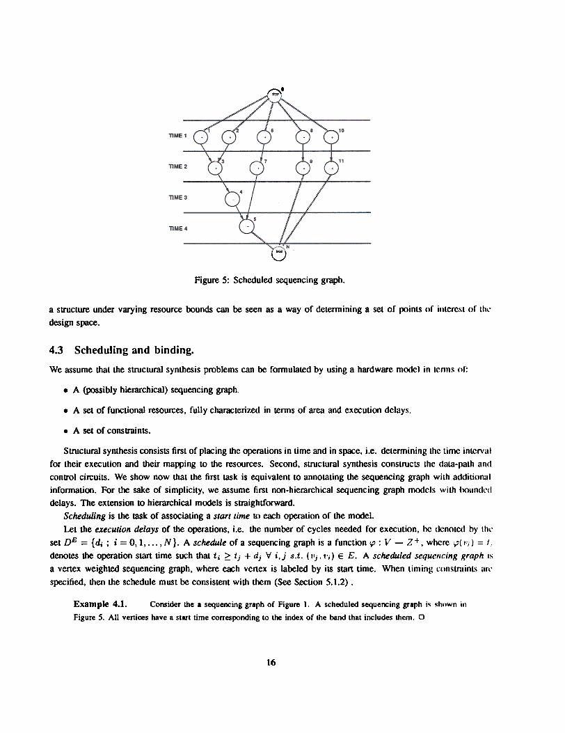
Scheduling is the task of associating a start time to each operation of the model.

Let the execution delays of the operations, i.e. the number of cycles needed for execution, be dcnotc<1 by thl'set DE = {di ; i = 0, 1, . . . , N}. A schedule of a sequencing graph is a function <p : V - Z +, where ;p( ";) = I,denotes the operation start time such that t i ~ t j + d j 'v' i, j s.t. (1'j, 1';) E E. A scheduled sequencing graph isa vertex weighted sequencing graph, where each vertex is labeled by its start time. When timing l:()nstruinl~ ,Ir('

specified, then the schedule must be consistent with them (See Section 5.1.2) .

Example 4.1. Consider dte a s~uencing graph of Figure 1. A schoouled sequencing graph i!i !ihllWn in

Figure 5. All vertices have a start time corresponding to the index of dte band that includes dtem. 0

16

Let us consider now the relations among the o~rations and the resources. We define type of an operationthe type of computation it ~rforms. It may be an arithmetic operation, such as addition or multiplicalion, or anapplication-specific operation. More formally we define the lype as a function T : V Y, whcrc \. is a s('.l of

enumerated types, such as {add,multiply,divide}.We can extend the notion of ty~ to the functional resources. We call resource-type set the set of resou.ce lypcs.

An operation can be matched to a resource when their type is the same. Obviously, a feasible implemcntalion requiresthat there are resources for all the types of operations in the s~ification. Therefore, without loss of generality, wecan identify the resource-type set with the set Y. In the sequel, we identify this set with its enumeration, i.c. we

set Y = {I, 2,..., nre,}, where n..e, = IYI. It is obvious that No-Operations do nOl require any binding lO anyresource. Therefore, when referring to a binding, we consider the set of vertices excluding the sou.ce and sink. i.<.'.

V = {vi;i = I,2,...,nop,}.Il is interesting to note thal there may be more than one operation with the same ty~. In this case, resourc(~

sharing may be applied. Similarly there may be more than one resource with the same type (e.g a ripplc-carry amI

a carry-look-ahead adder). In this case, a resource selection (or module selection) problem arises.A fundamental concept that relates operations to resources is binding. Il s~ifies which resourcc implemcnL';

an operation. A resource binding is a mapping 13: ~'-}' x Z+, where I3(Vi) = (t,j) denoles thallhe operationcorresponding to Vi E V, with type T(Vi) = t, is implemented by the jth instance of resou.ce typc I I: V ror l~ll'h

i = 1,2,...,nop,.A simple case of a binding is that of using dedicated resources. In this case, each operation is I)()und to on<.'

resource, and the resou.ce binding .B is a one-to-one function.

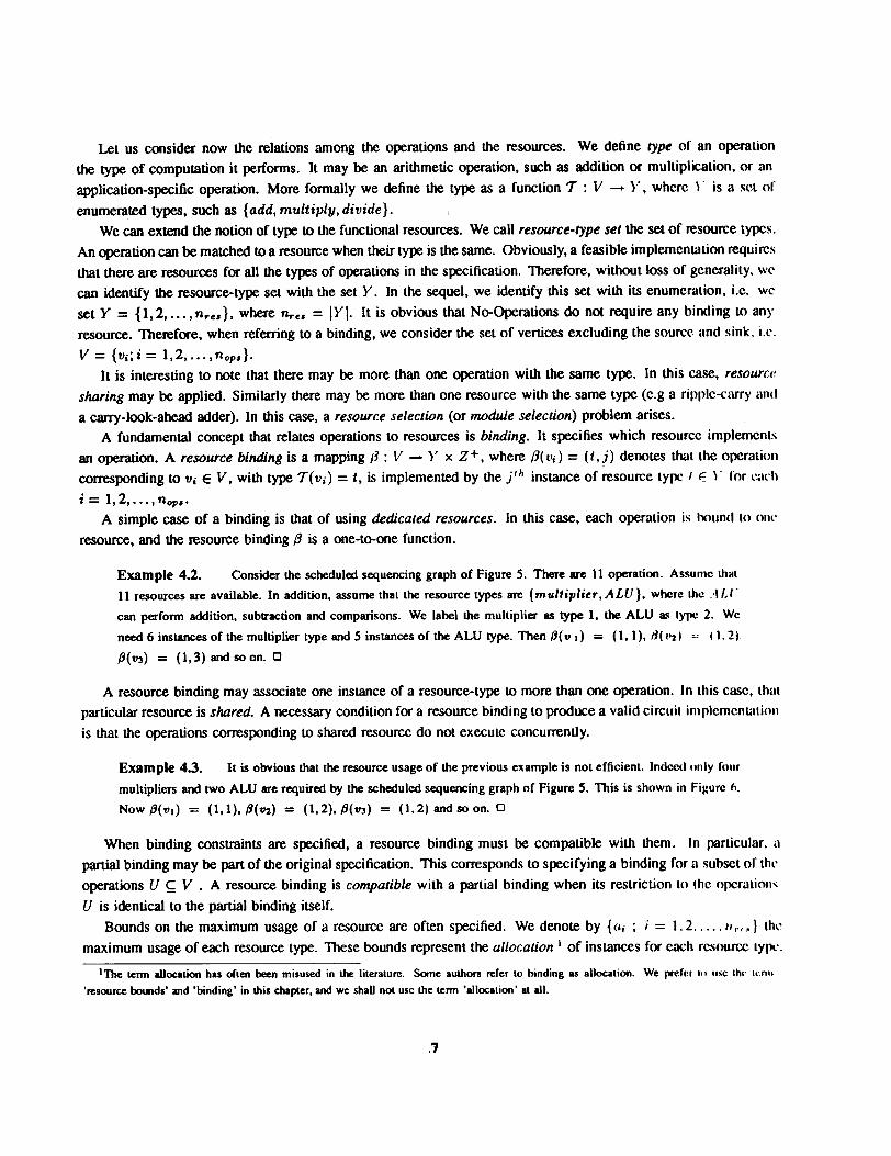
Example 4.2. Consider the scheduled sequencing graph of Figure 5. There are 11 operation. Assume thill

11 resources are available. In addition, assume that the resource types are {multiplier, A LlJ}, where lhe A L'"

can perform addition, subttaction and comparisons. We label the multiplier as type I, the ALU a.~ 1YJ1C 2. Wc

need 6 instances of the multiplier type and 5 instances of the ALU type. Then 8( v I) = (1, 1). III I'zl :0, 11.21.

.fJ(V3) = (1,3) and soon. 0

A resource binding may associate one instance of a resource-type to more than one operation. In this casc, thatparticular resource is shared. A necessary condition for a resource binding to produce a valid circuit impiemcnuilioll

is that the operations corresponding to shared resource do not execute concurrently.

Example 4.3. It is obvious that the resource usage of the previous example is not efficient. Indce<lllnly rour

multipliers and tWo ALU are required by the scheduled sequencing graph of Figure 5. This is shown in Figure h.

NOWfJ(Vi) = (1,1).fJ(v2) = (1,2)..8(v3) = (1,2) and so on. 0

When binding constraints are specified, a resource binding must be compatible with them. In particular, "partial binding may be part of d1e original specification. This corresponds to specifying a binding for" subset of thl'operations U ~ V , A resource binding is compatible with a partial binding when its restriction lO Ihe opcrulions

U is identical to the partial binding itself,Bounds on d1e maximum usage of a resource are often specified. We denote by {aj ; i = 1.2 '" r".} lhl~

maximum usage of each resource type. These bounds represent the allocation 1 of instances for each rcs(>urcc lyf)('.

IThe leon allocation has often ~n misused in the literature. Sane authors refer to binding as allocation. We prefl,r I., ""C .h.' \"",1

'KSoorce IxIunds' and 'binding' in this chapter, and we shall not usc the leon 'allocation' at all.

:7

,,'

Figure 6: Scheduled sequencing graph with resource binding.

A resource binding is compatible with resource bounds when I3(Vi) = (t, j) satisfies j :$ (It for cuch operation

Vi; i= l,2,...,nop..A scheduled and bound sequencing graph is a feasible structure when il satisfies all the constraints lhal arc

specified. We can now formalize the concept of the design space, by defining il as the collection of all fea.\'ibleStruclUres. Each feasible SlruclUre can be labeled with area and latency estimates using the criteria shown in Scclioll4.4. The former can be approximated by the sum of the areas of all the bound instances of each resource type. Thl'.latter can be computed as the start time of the sink vertex, i.e. tN, which corresponds to the length of the schc<lulc.

Il is important to remark that the present formulalion characterizes the design space in terms of area and latency.but it is also a funclion of the cycle-lime parameter. Indeed the dependency on the cycle-lime is due lO thecomputation of the execulion delays. By considering different values of the cycle-lime, the corresponding execulioll

delay vary and so do the corresponding feasible Slruclures.

4.4 Estimation.

Accurnte area and delay estimation is not a simple task. Much of the complexity of the structural synthc-'iis problemsis due to the difficulty of estimating the impact of a high-level decision on the structure of a circtlil on thc fin:lt

area and performance.Let us consider first resource-dominated circuits. A simple model is to assume that the area 'and the delay of l/1C

resource oominate, so that other factors can be neglected. This is a valid assumption in lhe case of DSP circuil~.The area estimate of a structure is the sum of the areas of the bound resource instances. Equivalenlly, the total

area is a weighted sum of the resource usage. A binding specifies fully lhe total area, but it is nOl ncccssary lOknow the binding to determine the area. Indeed, it is just sufficient to know how many instances of c8ch reSOIJrc{'

are used.The latency of a circuit can be determined by its schedule. Il is the start time t N of lhe sink operauon. In

the case that no constraints on the resource usage are imposed, then the latency can be derived clircctly from thl'

18

.sequencing graph by computing the length of the longest weighted path.

Let us consider now general circuits. and let us consider in more detail the area and delay eslimal ion problem

Registers. All data that is transferred from a resource to another across a cycle boundary must be SLorcd into someregister. An upper bound on the register usage can then be derived by examining a scheduled sequencing graph.This bound is in general loose, because the number of registers can be minimized, as shown in SccLion 6.4. The

binding information is needed for evaluating and/or performing the register optimization. Thereforc. Lhe accurnlC

estimation of the number of registers requires both scheduling and binding.The effect of registers on the evaluation of the cycle-time is easy to compute. In fact, their set up and propagation

delay times must be added to the propagation delays of the combinational logic. It is more efficient 10 consider"

reduced cycle-time in all the compuLaLions, that already discounts set up and propagation delays.

Steering logic. Steering logic affects the area and the propagation delay. While the area of multiplexers can

be easily evaluated, their number requires the knowledge of the binding. Similarly, multiplexers 8<ld propagationdelays to the resources, and the overall propagation delay must not exceed the cycle-time times thc CX('cution dc.liIY.

Busses can also be used to steer data. In this case appropriate models should be used.

Wiring. Wiring contributes to the area and to the delays. The wiring area overhead can be esLimatcd rromthe structure, once a binding is known, by using models that are appropriate of the physical design style or Lhcimplementation. The wiring delays are crucial. As in the case of steering logic, they add propagation delaysand we must insure that the overall propagation delay is bounded. Unfortunately, estimating the wiring requiresthe knowledge of the structure (i.e. the binding) as well as the placement of the physical implcmenLation or th('resources. Fast floor-planners have been used. Alternatively, statistical wiring models have been usc<l. In this ca~(',it has been shown that the average interconnection length is proponiooal to the total number of blocks to the "

power, where 0 .$ a .$ 1. The wiring delay and area track with the average interconnection IcngLh. We rcrer lh,'

interested reader to reference [47] for a detailed analysis of the wiring area and delay esLimalion.

Control logic. The control circuit conbibutes to the overall area and delay, because some conlrol signals can re part

of the crilical path. Recently, the interesl in synlhesizing control-dominaled circuils, such as some communicaliOlI

ASICs, has exJX>sed lhe imparLance and difficully of the problem. Simple models for estimaling lhe size of lhl~

conb"ol circuit can be based on the laLency. Consider bounded-lalency non-hierarchical sequencing grdphs. Read-only

memory based implementations of the control unils require an address space wide enough to accomm()(laLe all conLrol

sLeps and a word-length commensuraLe to the number of resources ooing conb"olled. Hard-wired implcmenlalions

can 00 modeled by finite-state machines with as many Slales as the lalency. UnfortunaLely, loose models may

provide loose bounds, because many optimization techniques can be applied to the controller, such as word-length

reduction by encoding and SlaLe encoding. In addilion, general models for sequencing graphs require more complex

conb"ol unils, as shown in Section 7, and eslimaLing accumLely the area and exlracting Lhe crilical slIh-path in lh('

conb"oller is a difficult task.

19

Scheduling.5Scheduling is a very important taSk in high-level synthesis. Whereas a sequencing graph denotes the partial orderof the operations to be performed, the scheduling of a sequencing graph determines the detailed starting time I()r

each operation. As a result, the degree of concurrency of the operations is determined by the scheduling taSk.The start time of the operations must satisfy the original dependencies of the sequencing graph. These depcn-

dencies limit the amount of parallelism of the operations, because any pair of operations related by a sequentialdependency (or a chain of dependencies) may not execute concurrently. As a limiting case, a schedulC{1 sequencinggraph may be such that the operations are fully serialized with respect to each other.

Scheduling a sequencing graph determines the concurrency of the resulting design, and therefore it affecl~ it..performance. By the same token, the maximum number of concurrent operations of a given type during the entireschedule is a lower bound on the number of required hardware resources for that operation. Therefore the choi<.~c

of a schedule affects also the area of the impJementation.The number of resources of a given t~ may be constrained from aoove. to satisfy some requiremenL~ relalC{1

to the physical design. For example, a circuit with a prescribed size may have at most one noating point multi-plier/divider. When resoun:e constraints are imposed, the number of operations of a given type that can overlap intime is limited by the number of resources of that type. Therefore tight bounds on the resources correlate to seri-alized implementations. A spectrum of solutions may be obtained by scheduling a sequencing graph with diffcrcnl

constraints. This is indicative of the possible area-performance trade-off points in the design space.We consider first sequencing graphs that are not hierarchical. We analyze the scheduling problem without

resource constraints in Section 5.1 and with resource constraints in Section 5.2. We consider then extensions to thc

modeJ in Section 5.3. We assume that execution delays are known, i.e. that aU operations have dala-indcpcndcnl

deJays. Exceptions are described in Section 5.1.3.

Scheduling without resource constraints.5.1

We consider here scheduling with no resource constraints. Let us denote by T = {t i ; i = O. I. . . . . N} lhc .\"tarl

time for the operations, i.e. a set of integer numbers denoting the cycle in which a particular o~ralion Slarl... Th('latency of the schedule is the numoor of steps to execute the entire schedule, or ~uiva1ently the starl lime of Lhl~sink tN. An unconstrained schedule is a set of values of Lhe Slart limes T, that satisfies the sequencing rclalionsrelations, i.e, ti ~ tj + dj Y i, j s.t. (Vj, Vi) E E. The minimum latency unconstrained schedulinx problem C(111

be defined as follows.

find{Inll

Definition 5.1 Given a set of operations V with integer delays DE and a partial order on the opcr(llion.\' ,an integer labeling of the operations If! : V --. Z +. such that ti = ip( Vi). ti ?; tj + dj V ;, j s.t. (Ij . '.j) r:

t N is minimum.

The unconstrained scheduling problem can be solved in polynomial time. Before considering the algorilhms for

its solution, we would like to comment on the relevance of the problem.It is obvious that the problem is important when the number of resources of a given type affecl~ only marginally

the overall quality of the solution. An example is the case in which the area cost of the resources is small comparc<1to the overhead of wiring and multiplexing the data to the resources being shared. In this case, the use of dedicalc<1resources is preferred. A similar situation is when the operations require resources of different ly~s, so thaI Ihl~r('

is just a resource for each operation.

20

Unconstrained scheduling is also used when the decision on resource sharing and their binding to operations i~done prior to scheduling. In this case, the area cost of an implementation is defined before and inde~ndently fromthe scheduling step. Eventually unconstrained scheduling can be used to derive bounds on latency for conslraine<1problems. By relaxing the resource constraints, a lower bound can be computed, because the minimum latency ofa schedule under some resource constraint is obviously at least as large as the latency computed with unlimitedresources. Conversely, by assuming dedicated resources, an upper bound can be computed. These bounds arc u~cflll

in simplifying the solution of the constrained problem.

5.1.1 The ASAP and ALAP scheduling algorithms.

We consider here die minimum latency scheduling problem. This problem can be solved in polynomial limeby topologically sorting die vertices of the sequencing graph. This approoch has been called As Soon As Possible

(ASAP) scheduling algoridlm, because the start time for each operation is the minimum allowed by lhc (k-,pcndcncil's.

The algorithm can be summarized by the following program:

ASAP (G(V,E»

Schedule Vo by setting to = 0;

repeat {Select a vertex Vi whose predecessors are all scheduled;Schedule Vi by setting ti = max tj + dj;

j..I(Vj.Vi)EE

}until (v N is scheduled)

The computational complexity of the algorithm is O(IEI).We consider now the case in which a schedule must satisfy an upper bound on the latency, denol('.d by ,\, Thl'

problem may be solved by executing the ASAP scheduling algorithm and verifying thal t N ~ '\.

If a schedule exists thal satisfies the latency bound '\, il is possible then to explore the range of values or lhl'start times of the operations thal meelthe bound. The ASAP scheduling algorithm yields the minimum values ofthe start times. A complementary algorithm, the As Lale As Possible (ALAP) scheduling algorithm provides lh\'

corresponding maximum values. Here is a description of the algorithm.

ALAP( a(v, E),~){

Schedule VN by setling tN = A;

repeat {Select vertex Vi whose successors are all scheduled;Schedule Vi by selting ti =, min i.j - di ;

j61(tli,"i)EE

until (v N is scheduled) ;

21

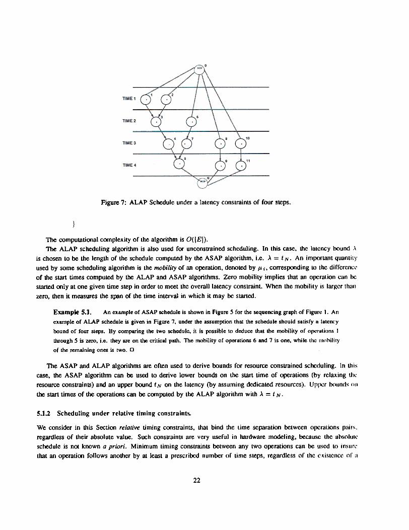
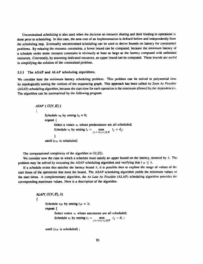
Figure 7: ALAP Schedule under a latency constraints of four steps.

The computational complexity of the algorithm is O( lEI).The ALAP scheduling algorithm is also used for unconsttained scheduling. In this case, lhe laLcncy bound ,\

is chosen LO be the lenglh of lhe schedule computed by lhe ASAP algorithm, i.e. >. = t. N. An imJ)(>fLant quanLity

used by some scheduling algorilhm is lhe mobility of an operation, denoted by Jl i, corresponding to the dirrerencrof lhe start times computed by the ALAP and ASAP algorithms. Zero mobility implies that an o~ralion can bcstarted only alone given time step in order to meet the overall latency conslf8jnt. When the mobility is larger thanzero, lhen it measures lhe span of the time interval in which it may be started.

Example 5.1. An example of ASAP schedule is shown in Figure 5 for the sequeocing graph of Figure I. An

example of ALAP schedule is given in Figure 7, under the assumption that the schedule should salisry 8 lalCrK'y

bound of four steps. By comparing the two schedule, it is possible to deduce that the mobility or operalions I

through 5 is zero, i.e. they are on the critical path. The mobility of operations 6 and 7 is one, while Ihe mohility

of the remaining ones is two. 0

The ASAP and ALAP algorithms are often used to derive bounds for resource constrained scheduling. In thiscase, the ASAP algorithm can be used to derive lower oounds on Lhc start time of opera Lions (by relaxing Lh~resource constraints) and an upper bound tN on the latency (by assuming dedicated resources). UPlx..r \)(Iuncls (IIIthe start times of the operations can be computed by Lhe ALAP algoriLhm wiLh ;\ = tN.

5.1.2 Scheduling under relative timing constraints.

We consider in this Section relative timing constraints, that bind the time separation between operations pairs.regardless of their absolute value. Such constraints are very useful in hardware modeling, because the absolulcschedule is not known a priori. Minimum timing constraints between any two operations can be used to insur('that an operation follows another by at least a prescribed number of time steps, regardless of the {~xislenC{~ of ..

22

dependency between them. It is often also imponant to limit the maximum distance in time between two operationsby means of maximum timing constraints. The combination of maximum timing constraints with the minimum

timing constraint permits us to specify the exact distance in time between two oJx:rations and, as a special casc.their simultaneity. For example, consider a circuit with two independent streams of oJx:rations, that arc constrainedto communicate simultaneously to the external circuits by providing two pieces of data at two interfaccs. The cyclcin which the data are made available is irrelevant although the simultaneity of the operations is important. Thisrequirement can be captured by setting a minimum and a maximum timing constraint of zero cyclcs bctwccn the

two write operations.We define more formally the timing constraints as follows:

. A minimwn timing consb"aint loj ~ 0 implies that: t j ~ tj + lij

A maximum timing consb"aint tlij ~ 0 implies that: tj ~ ti + tlij

A schedule under timing constraints is a set of start times for the operations satisfying the requirements slllt!.'.!1

in Definitions 5.1 and 5.3. and in addition:

Vlij~ tj + Iii

2)ti ~ tj + Uij VUij

A consistent modeling of minimum and maximum timing constraints can be done by means of a conslfaintgraph Gc(Vc. Ec) , that is an edge-weighted directed graph derived from the sequencing graph as follows. Theconstraint graph Gc(Vc. Ec) has the same vertex set as G(V, E) and its edge set includes the edge set P. Suchedges are weighted by the the delay of the opernlion con-esponding to their tail. The weight on the cdgc (I';. "j) isdenoted by wii' Additional edges are related to the timing constraints. For every minimum tim jng conslfaintl iJ .we add a forward edge (Vi, Vi) in the constraint grnph with weight equal to the minimum value 1" ij = lij :,::: O. Forevery maximum liming constraint uii' we add a backward edge (vi, 'I';) in the constraint grclph with weight equalto the negative of the maximum value Wii = -USi $ 0, because ti $ I; + uii implies I; :,::: Ij - "ij. Note that

the overall latency constraint can be modeled as a maximum liming conslfaint UO,N between the !iOllrCe and sink

vertices.

Example 5.2. Consider the example in Figure 8, A minimum timing constraint requires operation "4 II) takc

place at least lOt = 3 cycles after operation Vo has started, A maximum timing constraint requires operati()n 1'3 II)

take place at most U31 = 3 cycles after operation' VI has started. Note that the constraint graph has 8 h.I(.'kwarci

edge with negative weight (e.g. -3). 0

The ..-esence of maximum timing constraints may prevent the existence of a consistent schedule, as in the caSl'.of the latency constraint. In particular, the requirement of an upper bound on the time distance beLween the S~lrltime of two operations may be inconsistent with the time required to execute the first operation, plus possibly thetime required by any sequence of operations in between. Similarly, minimum timing constraints may also conllici

with maximum timing constraintA criterion to determine the existence of a schedule is to consider in turn each maximum timing constrainl

Uij. The longest weighted path in the constraint graph between Vi and Vj (that determines the minimum separationin time between operations Vi and Vj) must re less than or equal to the maximum timing conslrail11 It Ii, As a

23

00

MNTIME3

I

MAXTIME

3..a

Figure 8: Example of a constrainl graph, wilh a minimum and a maximum timing constraint The n"mher insidr ,I

vertex represenls ils execution delay.

consequence, any cycle in the constraint graph going through (v j , Vi) must have negative or zero weight. TherefoR',a necessary condition for the existence of the schedule is that the constraint graph does not have slricLly pc)siLiv('

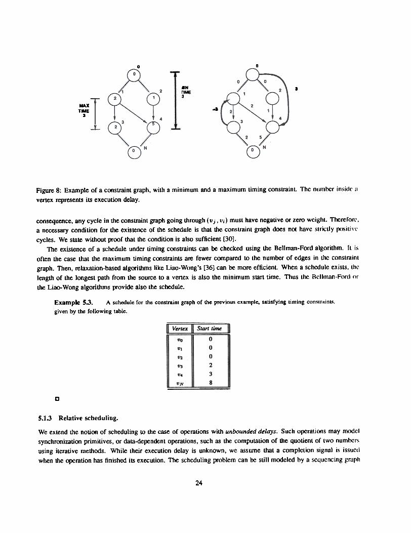
cycles, We state without proof that the condition is also sufficient [30].The existence of a schedule under timing constraints can be checked using the Bellman-Ford algorithm, It is

often the case that the maximum liming constraints are fewer compared to the number of edges in the constrdinLgraph. Then, relaxation-based algorithms like Liao-Wong's [36) can be more efficient. When a schedule exists, thelength of the longest path from the source to a vertex is also the minimum start lime. Thus Lhe Bc.llman-Ford or

the Liao-Wong algorithms provide also the schedule.

Example 5.3. A schedule for the constraint graph of the previous example, satisfying timing conslrainL~.

given by the following table.

Vertex II Start time

000

23

8

vo

VI

V2.

VJ

V4

VN

0

5.1.3 Relative scheduling.

We extend the notion of scheduling to the case of operations with unbounded delays. Such operations may modelsynchronization primitives, or data-dependent operations, such as the computation of the quotient of two numbersusing iterative methods. While their execution delay is unknown, we assume that a completion signal is issuc<1when the operation has finished its execution. The scheduling problem can be still modeled by a sequencing grdph

24

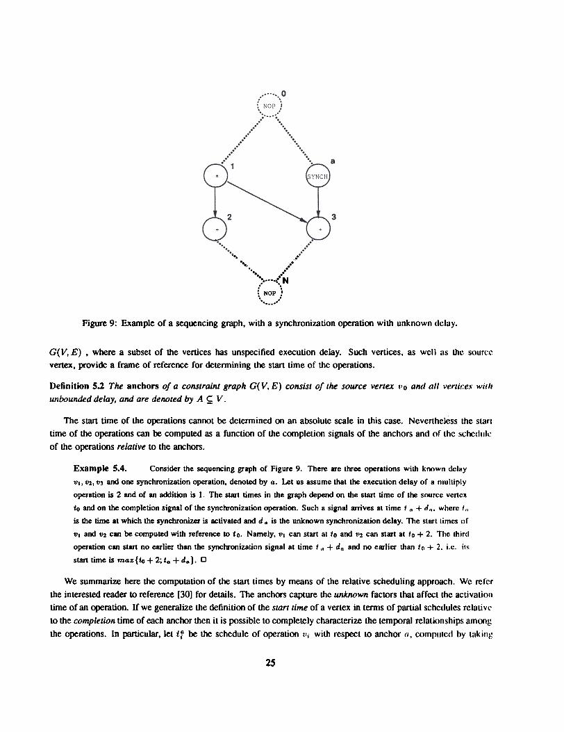
"..0 .."...

.. .... ... .,,"" N: .... NOP I. '. "

"... ..

Figure 9: Example of a sequencing graph, with a synchroni7.ation operation with unknown delay.

G(V, E) , where a subset of the vertices has unspecified execution delay. Such vertices. as well as the S()Ur<':l~vertex, provide a frame of reference for determining the start time of the operations.

Definition S.2 The anchors of a constraint graph G( V. E) consist of the source vertex Vo and all vertice.~ withunbounded delay. and are denoted by A ~ V.

The stan time of the operations cannot be determined on an absolute scale in this case. Nevertheless the starttime of the operations can be computed as a function of the completion signals of the anchors and of the schedul('of the operations relative to the anchors.

Example 5.4. Consider the sequencing graph of Figure 9. There are three operations with known delity

VI, tI2, V3 aOO one synchronization operation. denoted by a. Let us assume that the execution delay of a multiplyoperation is 2 and of an addition is 1. The Slarl times in the graph depend on the start time of the source vertex

to and on the completion signal of the synchronization operation. Such a signal arrives at time I" + d". where In

is the time at which the synchronizer is ~tivated and d" is the unknown synchronization delay. The slarllimes of

VI and tI2 can be computed with reference to to. Namely, \'1 can start al 10 and .'2 can start at to + 2. The third

operation can start no earlier than the synchronization signal at time t" + do and no earlier than 1(1 + 2. i.c. il~

start time is max{to + 2; to + do}. 0

We summarize here the computation of the start times by means of the relative scheduling approach. We refcrthe interested reader to reference [30] for details. The anchors capture the unknown factors that affect the activationtime of an operation. If we generalize the definition of the start time of a vertex in terms of partial schedules relativeto the completion time of each anchor then it is possible to completely characterize the temporaJ relalionships amongthe operations. In particular, let tf be the schedule of operation Vi with respect to anchor (I, complllc<1 by ulkin~

2S

the subgraph induced by the soccessors of a, assuming that a is the source of the graph and that all anchors havezero execution delay. Let do be the unbounded unknown execution delay of anchor a. The start Lime of a vertex

Vi is computed recursively as follows:

ti = max{ta + da + tf} (3)aEA

In practice, a subset of the anchors .4, called relevant anchor set is sufficient to determine the start time (30J.Note that if there are no operations with unbounded delays, then the start times of all o~rations will be specifi~1

in terms of time offsets from the souoce vertex, which reduces to the traditional scheduling formulation.A relative schedule is a collection of schedules with respect to each anchor, or equivalently a set of offsets with

respect to the relevant anchors for each vertex. From a practical point of view, the start times of Eq. 3 cannot bt'.

computed. However, the offset values and the anchor completion signals are sufficient to construct a control circuit

that activates the operations at the appropriate times.Relative scheduling can be performed under liming constraints. The constraint graph fonnulalion slill applies

although the weights on the edges whose tails are anchors are unknown. Also in this case a schedule mayor maynot exist under liming constraint It is importanllo be able to assess the existence of a schedule for any value of

the unbounded delays, because these values are not known when the schedule is computed. We call a sequencinggraph well-posed when il has this important property. Relative scheduling can be applied lO well-posed graphs. to

determine the start times of the operations. An important issue, is the verificalion of the well-posC(lncss property.

Related algorithms are reported in reference [30].

Scheduling with resource constraints.5.2

Scheduling under resource constraints is an important and difficult problem to solve. Resource constraints stemfrom the fact that they give a rough measure of the area utilization, for some applications. Consider for exampleDSP filters, that use extensively bit-parallel addition and multiplication. The overall area of the implementation isaffected mainly by the number of resources. Therefore, a maximum number of adders and of multipliers can h<...required to insure physical feasibility of the implementation or as a way of determining an area-performance Lrade-off point in the design space. Ideally, the entire design space can be characterized by solving the scheduling problcmunder different resource constraints. In practice two difficulties arise. FirsL, the resource-constrained schedulingproblem is intractable, and only near-optimal solutions can be found for problems of reasonable size. Second, Lhcarea-performance b'ade-off points are affected by other quantities, related to the area and delay of militiplexcrs. thl.'

length of the wires and the number of registers.A resource-constrained scheduling problem is one such that the number of resources of any given Lype arc

bounded from above by a set of integers {aA:; k = 1,2,..., nrel}' Therefore the operations are scheduled in sucha way that the number of executing operations of a given type in every schedule steps does not excC{'(\ thr hc)lIrnl.

The minimum latency resource-constrained scheduling problem can be defined as follows.

Definition 5.3 Given a set of operations V with integer delays DE. a partial order on the operation.~ I:.', and upperbounds {ak; k = 1,2,..., nre.}, find an integer labeling of the operations tp : V --+ Z + such tllt,t f i = ~(";).

ti ~ tj + dj V i,j B.t. (Vj,Vi) E E. I{ViIT(tl;) = k and ti .s: j < ti + di}1 .s: ak for each operation-type

k = 1,2,..., nrc. and schedule step j. and t N i.\" minimum.

26

When all the resources are of a given type (e.g. ALUs), then the problem reduces to the classical mulLiproccssorscheduling problem. The minimum latency mulLiproccssor scheduling problem is intractable.

5.2.1 The Integer Linear Programming model.

A fonnal model of the scheduling problem under resource constraints can be achieved by using binary decisionvariables with two indices: X = {XiI; i = 1,2, N; 1= 1.2,..., L}. The number L represents an upper boundon d1e latency, because d1e schedule latency is 'unknown. The bound can be computed by using a fast heurisLi~scheduling algorid1m, such as a list scheduling algorithm (Section 5.2.2). In the sequel, we denote the summationsover all operations as Li (instead of L~o) and d1ose over all schedule steps as LI (instead of 2::f= I) for the sake

of simplicity.The binary variable, XiI, is 1RUE (i.e. 1) only when operation Vi SIarlS in step I of d1e schedule, i.e. I = Ii.

Equivalently, we can write XiI = 6(ti, I), where ft(p, q) is d1e Kronecker delta notation. Therefore Lhr !itarllime ofoperation Vi can be slated in tenns of XiI as: ti = LII . XiI.

The following model expresses d1e constraints on d1e schedule in terms of the binary variables. Firsl, operations

start only once:(4LZtl = 1 i= 1,2, N

I

Second, the sequencing relations represented by G(V, E) must be satisfied. Therefore, it ~ ij+dj Vi, j tr.f .(rJ

E implies:

}:1,zil?}:I'Zjl+dj i,j=1.,2,...,.lV a.t,(vj,vi)EE (5)I I

jL :}: Zil$a" k=I,2, nrt.: j=O,I,...,tN (6)

11111 such that

= 1 ;=1,2,..min

LXi,,N ~t

N 8.t~VJ' Vi) E EL I. Zil - L I. Zjl - djI I

0 i,j= 1,2. (8)~

;

L L.,.,.T(Vi)=i 1=;-";+1

4t k= 2, Rr..; j=O,l,.. (9)<- INZit

The choice of the norm of vector i to be minimized relates to slightly different goals. The infinity normcorresponds to minimize the maximum entry of t, i.e. tN. Therefore the objective function to minimize is:

27

Third, the resource bounds must be met at every schedule time step. An operation Vi is ex~uling attimc stcl)j when E1=;-di+l Zil = 1. Therefore the number of all the operations ex~uting at step j of tYI'IC t. must hl~lower than or equallo the bound a k. Namely:

i $.t.7(tli)=k I=j-di+l

Let us denote by .t the vector whose entries are the start times. Then, the minimum latency schc<llIling pmhlcill

under resource constraints can be stated as follows:

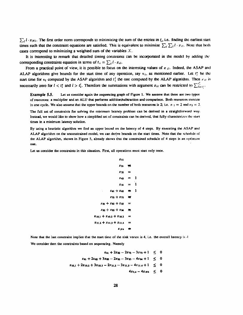
E,l. XNI. The first order nonn corresponds lO minimizing the sum of the enlries in t. i.e. finding thc earliest starttimes such lhalthe consuainl equations are satisfied. This is equivalenllO minimize Ei E,l. ;ri/. Notc Lhat bothcases correspond lO minimizing a weighted sum of lhe variables ".

Il is inleresting lO remark lhal detailed timing conslrainlS can be incorporaled in the model hy adding Lhl'corresponding consb'ainlS equation in lenDS of t i = E,l. XiI.

From a practical point of view. il is possible lO focus on the inleresting values of X il. Indeed. the ASAP and

ALAP algorithms give bounds for the start time of any operation. say Vi. as mentioned earlier. Lel if be th<'.start time for Vi computed by the ASAP algorithm and t ~ the one computed by the ALAP algorithm. Then J' i/ is,necessarily zero for I < t: and I > t~. Therefore the summations with argument XiI can be reslricLed 102:::;";',;.

Example 5.5. Let us consider again the s~uencing graph of Figure 1. We assume that there are two typesof resources: a multiplier and an ALU that performs addition/SuWaction and comparison. Both resources execulcin one cycle. We also assume that the upper bounds on the number of both resources is 2; i.e. a J = 2 and /12 = 2.

The full set of constraints for solving the minimum latency problem can be oorived in a straightforward way.Instead. we would like to show how a simplified set of constraints can be derived, that fully characterize~ IlIl~ ~lart

times in a minimum latency solution.

By using a heuristic algorithm we find an upper bound on the latency of 4 steps. By execuling lhc ASAP and

ALAP algorithm on the unconstrained model. we can de~ve bounds on the start times. Note that the schCllulc orthe ALAP algorithm, shown in Figure 5, already shows that the constrained schedule of 4 steps is an optimum

one.

Let us consider the constraints in this situation. First, all operations must starl only once.

%11

%21

%31.

%43

.=

I

1

1

=x~ =

;1:61 + %62

xn + %:73

X81 + XG, + Xo

Xn + ;1:93 + X,.

%10,1 + Xl0.2 + %10.3

%11.2 + Xll.3 + %11..

%N.

~.=.==.

Note that the last constraint implies that the start timc of the sink vertex is 4, i.e. the overall latency i~ ,I

We consider then the constraints based on sequeocing. Namely

~

~~

~

%61 + 2x. - 2x'/2 - 3xn + 1

XII + 2xa. + 3%., - 2xga - 3X93 - 4XM + 1

XI0,1 + 2xl0,1 + 3XI0,3 - 22:11,1- 3%11,3 - 4XII.4 + 1

4X5.4 - 4%114

28

0

0

0

0

0

0

2za + 3s" + 4XM - 4SN4 S2s11,1 + 3Z11,3 - .Xll,4 - 4ZN4 S

Finally we consider the resource constraints:

&'11 + %21 + %61 + %.1

&'D + %C + %72 + %a

%73 + %.,

.1:10.1

.1:n + .1:10.2 + .1:11,2

.1:43 + .1:",2 + 2:10.3,2 + .1:11.3

.1:,. + .1:94,2 + .1:11.4

~ 2

~ 2~ 2

~ 2~ 2

~ 2~ 2

Any set of start times satisfying these constraints is valid. For the sake of illustration, let us assume oow Ihal lhc

heuristic algorithm would have given us a bound on lhe lalency of 5 SlepS. We want to find out if lhe Ixlund is

tight. In this case, the larger mobility of lhe operalions would lead lO a larger set of constraints. We leave as an

exercise to the reader to derive the constraints equation. We just remark that the uniqueness conslrainl on Ihc slarl

time of the sink vertex would be XN4 + XN5 = 1 and the objective funclion would be min (4. x N4 + 5. ",'115).

Therefore, assuming that all the new constraint equations are satisfied. the optimum solution would impl~ .I ,Y4 = IaM X N5 = 0, i.e. a schedule of four steps. 0

The dualSo far we have considered the minimum-lalency scheduling problem under resource con.\'lrainl.\'.problem is the minimum-resource scheduling under lalency constrain l.\', that can re formalized as follows:

man

LxiII

II!!! I 8uch that

= 1 i=l,2, N

L,0 i,j = 1,2,...,N 8.t.(Vj,Vi) E E>~

LiZ;J;

~ j =0, tNs

where the lasl consu-aint equation bounds the latency instead of the resource usage.Note the choice of the nonn of vector .Go to be minimized relates again to slightly different goal!;, for cxampl('

the sum of the resources. A slightly different formulation may incorporate weights for the resource!;.

Example 5.6. Let us consider again the sequencing graph of Figure 1. with the assumptions used in theprevious example. Let us assume that the multiplier costs five times as much as an ALU in terms of IITl..a. Wcassume that an upper bound on the latency is ~ = 4.

The uniqueness constraints on the start time of the operations and the sequency dependency constraint~ arc thcsame of the previous example. The resource constraints are in terms of the unknown variables (/ I 811<111 ~.

~Zu + S2J + Z61 + %11

29

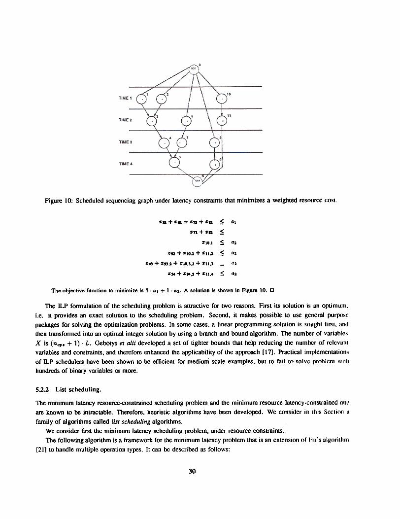
Figure 10: Scheduled sequencing graph under latency constraints that minimizes a weighted rcsmlrcc l~OSI.

~». + ~G. + %72. + ~G.

%73 + ~13

$:

$:

$:

$:

41

Xl0,l 42,

%a + %10.2 + %11.2

SO + Z".2 + 2'10,'.2 + ZII"

Z,. + Z,..2 + ZII.4

U2

a2--

~ az

The objective function to minimize is 5.41 + 1 .41. A solution is shown in Figure 10. 0

The ll..P fonnulation of the scheduling problem is attractive for two reasons. First its solution is an opLimum.i.e. it provides an exact solution to the scheduling problem. Second, it makes )X>ssible to use general purJX}S('packages for solving the optimization problems. In some cases, a linear programming solution is sought first, andthen transfonned into an optimal integer solution by using a branch and bound algorithm. The numrer of variablesX is (nop. + 1) . L. Gebotys et alii developed a set of tighter bounds that help reducing the numrer of relevam

variables and conSb"aints, and therefore enhanced the applicability of the approach [17]. Practical implementationsof ll..P schedulers have been shown to be efficient for medium scale examples, but to fail to solve rrobl('.m with

hundreds of binary variables or more.

5.2.2 List scheduling.

The minimum latency resource-eonstrained scheduling problem and the minimum resource latency-eonstraincd oneare known to be intractable. Therefore, heuristic algorithms have been developed. We consider in this Sccti()n il

family of algorithms called list scheduling algorithms.We consider first the minimum latency scheduling problem, under resource conSb"ainls.The following algorithm is a framework for the minimum latency problem that is an extension or HII'S algorithm

[21] to handle multiple operation types. It can be described as follows:

30

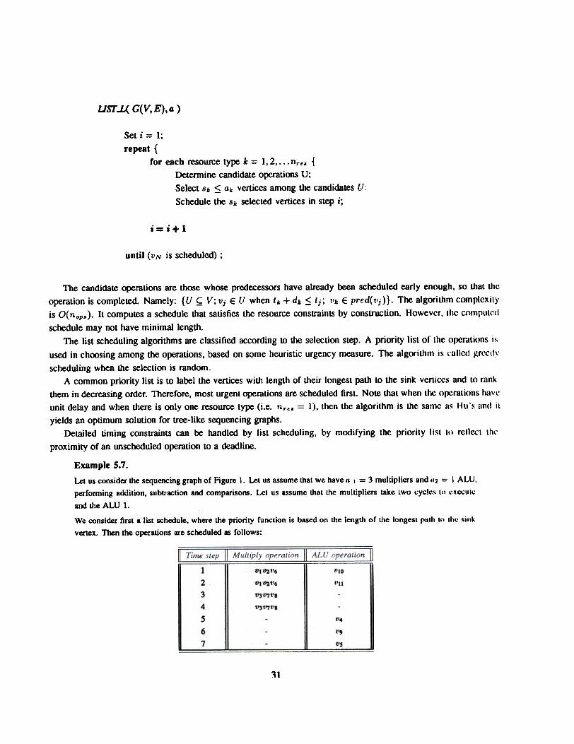
usr.L( G(V, E), CJ )

Set i = 1;

repeat {for each resource t~ k = 1,2,... "reI {

Detemline candidate operations U;Select SA: ~ aA: vertices among the candidates U:Schedule the SA: selected vertices in step i;

i=i+l

until (v N is scheduled) ;

The candidate operations are those whose predecessors have already been scheduled early enough, so that thcoperation is completed. Namely: {U ~ V;Vj E [I when t'k + dk .$ tj; "'k E pred(vj)}. The algorithm complexity

is O(nop.). It computes a schedule that satisfies the resource constraints by construction. However, Ihc oomputcd

schedule may not have minimal length.The list scheduling algorithms are classified according to the selection step. A priority list of the operations is

used in choosing among the operations, based on some heuristic urgency measure. The algorithm is l'allc<1 grl'{:dy

scheduling when the selection is random.A common priority list is to label the vertices with length of their longest path to the sink vertices and to rank

them in decreasing order. Therefore, most urgent operntions are scheduled first. Note that when Lhc o~rations havl'unit delay and when there is only one resource type (i.e. n,.". = 1), then the algorithm is the same as Hu's and iL

yields an optimum solution for tree-like sequencing graphs.Detailed timing constraints can be handled by list scheduling, by modifying the prioriLy list tl) rel1ccL Lhl'

proximity of an unscheduled operation to a deadline.

Example 5.7.Let us consider the sequencing graph of Figure I. Let us assume that we have a I = 3 multipliers and '/2 = I ALU.

performing addition, su~action and comparisons. Let us assume that the multipliers take lwo cyclc!O III ~Xcc.:Ulc

and the AW 1.

We consider first a list schedule, where the priority function is based on the length of the longest path ttl Ihc !Oink

vertex. Then the operations are scheduled as follows:

tll/11t16

tlllOZt'6

tl31'7t'8

tl3t'7t'8

('10

(III234

567

t'4

t'9

tiS

~1

It is possible to verify that the schedule has minimum latency.

Consider now a greaiy scheduling approach. where operations v 2. V6, va are scheduled at the first step. Then, Ihe

schedule would require at least 8 steps, arKl it would nol be optimal. 0

List scheduling can also be applied to the latency-constrained minimum resource problem. In this case, the slackof an operation can be used to rank the operations, where the slack is the difference between Lhc latcst possiblestart time computed by an ALAP schedule and the current schedule step under consideration. The lower the slack,Lhe higher the urgency in the list is. Operations with zero slack are always scheduled. The remaining ones arcscheduled only if Lhe number of required resoun;es does not increase. Ties are broken using the urgency list.

UST.R( G(V, E), ). )

fCompute the earliest possible schedule by ASAP ( G(V, E»;Compute the latest possible schedule by ALAP (G(V,E),~);Set i = 1;

repeat {Compute the slacks of the operations;for each resource type k = 1,2,... "reI {

Schedule at step i the candidate operations with zero slack;Schedule at step i the candidate operations that do not require addilH)nal reSOIlrC('S

i = i + 1;

until (VN is scheduled) ;

}

Overall list scheduling algorithms have been widely used in synthesis systems. The experimenUlI results haveshown that the algorithm can be applied to large graphs. Solutions have been shown not to be much diffcrcnL in

latency from the optimum ones, for those (small) examples whose optimum solutions are known.

5.2.3 Other heuristic scheduling algorithms.

Several other heuristic scheduling algorithms have been proposed. Some are derived from software design tech-niques. Example of these algorithms are trace scheduling and perco/alion scheduling. The latler has been usedin different forms in various synthesis systems, even though some of its implementations were more restrictive in

scope and power than the original algorithm. Percolation scheduling uses a transformational approach, thal movesoperations from one control step to another. This has to be contrasted to the list and force-direclccl schccllllingapproaches, that are constructive.

A commonly used heuristic scheduling algorithm is force-directed scheduling, that was proposed by Paulinand Knight [45]. It can be considered as an extension to the list scheduling approach, where opcralions are slillscheduled for increasing time steps. The major contribution of the force-directed scheduling approach is that il

considers a global function in the candidate selection process, namely the probability distribution of operation-lyreacross the schedule. This function mooels the likelyhood that a resource is used at any given step. A IInifoml

32

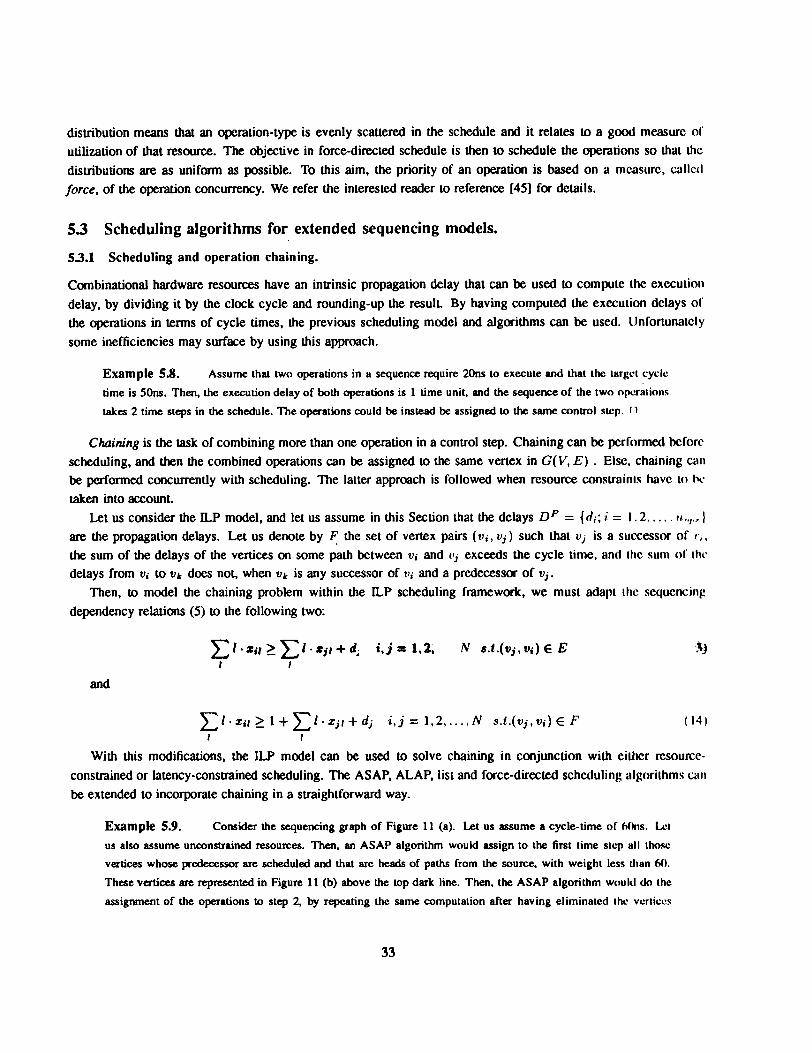
distribution means that an o~ration-type is evenly scattered in the schedule and it relates to a good measure ofutilization of that resource. The objective in force-directed schedule is then to schedule the operations so thal thcdistributions are as uniform as possible. To this aim, the priority of an operation is based on a measure, calleclforce, of the o~ration concurrency. We refer the interested reader to reference [45] for details.

Scheduling algorithms for extended sequencing models.5.3

Scheduling and operation chaining.5.3.1

Combinational hardware resources have an inttinsic propagation delay that can 00 used to compute the executiondelay, by dividing it by the clock cycle and rounding-up the result By having computed the execution delays of

the operations in terms of cycle times, the previous scheduling model and algorithms can be used. Unfortunately

some inefficiencies may surface by using this approach.

Example 5.8. Assume that two operations in a sequence require 2Ons to execule and lhal lhe largct cycle

time is 5Ons. Then. the execution delay of bolh operations is 1 time unit. and the sequerx:e of the two opcratiol1s

lakes 2 time steps in the schedule. The operations could be instead be assjgned to the same conuol step. 11

Chaining is the task of combining more than one operation in a control step. Chaining can be performed bcforcscheduling. and then the combined operations can be assigned to the same vertex in G(V, E) . Else, chaining cunbe performed concurrently with scheduling. The latter approach is followed when resource constraints have LO hl'

taken into account.Let us consider the ll..P model, and let us assume in this Section that the delays DP = {d;; ; = 1.2 1/.,.,...1

are the propagation delays. Let us denote by r: the set of vertex pairs (Vi, Vi) such that v j is a su(,'Cessor of I.,.the sum of the delays of the vertices on some path between Vi and Vj exceeds the cycle time, and thc sum of th(.delays from Vi to Vt. does not. when Vt. is any successor of Vi and a predecessor of vi.

Then, to model the chaining problem within the ll..P scheduling framework. we must adapt lhc sequencingdependency relations (5) to the following two:

Llo,zil ~ L1.,zjl + d,I ,

i,j: 1,2, N s.t.(vj,vi)EE ~j

and

LI'Zil~l+LI'Zj,+dj i,j=1,2, N s.t.(vj,vi)EF (14)I ,

With this modificalions, the ILP model can be used LO solve chaining in conjunclion with eill1Cr rcsourcc-conslrained or latency-consb"ained scheduling. The ASAP, ALAP, lisl and force-directed scheduling algorithms al"be exlended LO incorporale chaining in a sb"aighlforward way.

Example 5.9. Consider the sequencing graph of Figure 11 (a). Let us assume a cycle-time of 6(lns. Let

us also assume unconstrained resources. Then, an ASAP algorithm would assign to the first time step all thosc

vertices whose predecessor are scheduled and that arc heads of paths from the source, with weight less tllan (,().

These vertices are represented in Figure 11 (b) above the top dark line. Then. the ASAP algorithm wou Id do the

assignment of the operations to step 2, by repeating the same computation after having eliminated thc VI..'fticc!;

33

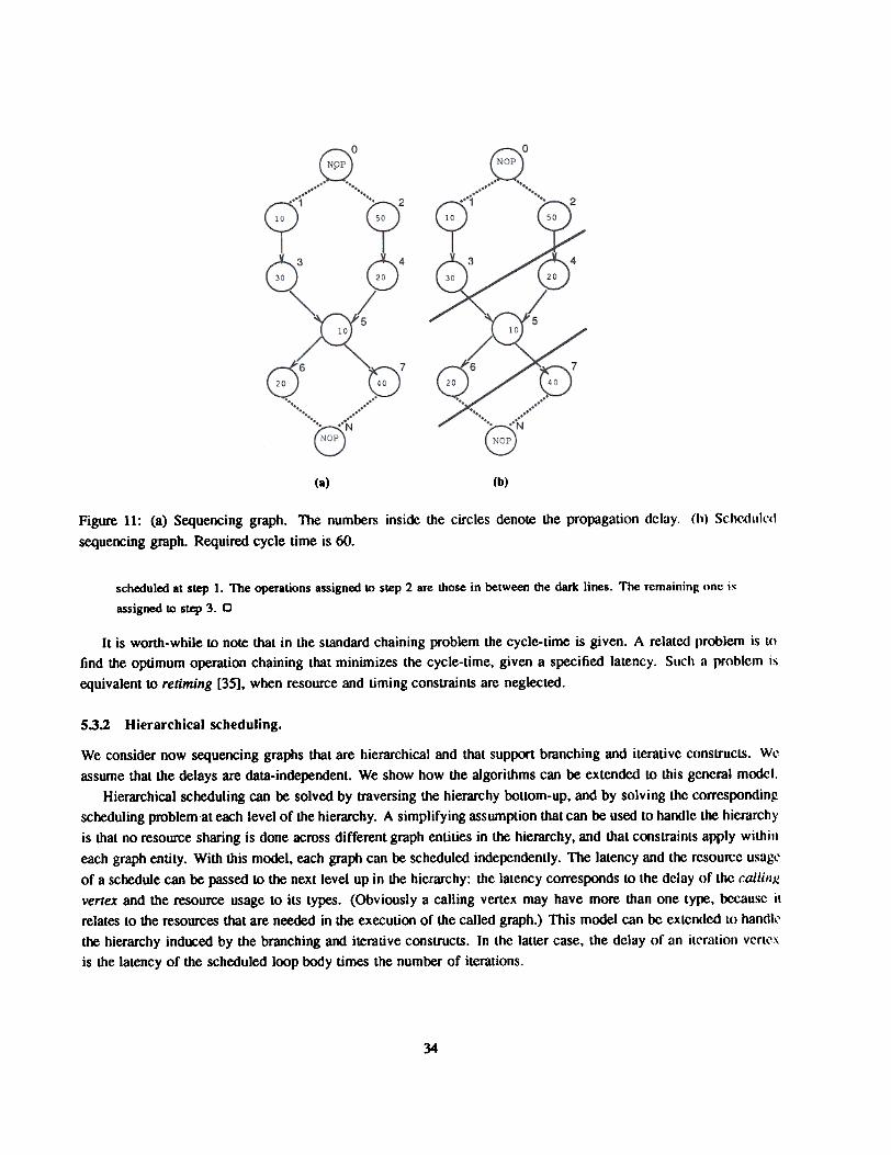
(b)(a)

Figure 11: (a) Sequencing graph. The numbers inside the circles denote the propagation delay. (h) Schcclllll'{\

sequencing graph. Required cycle time is 60.

scheduled at step 1. The operations assigned to step 2 are those in between the dark lines. The remaining (me i~

assigned to step 3. 0

It is worth-while to note that in the standard chaining problem the cycle-time is given. A related problem is lOfind the optimum operation chaining lhal minimizes the cycle-time, given a specified latency. Such a problem is

equivalent to retiming [35], when resource and timing constraints are neglected.

Hierarchical scheduling.5.3.2

We consider now sequencing graphs that are hierarchical and that support branching and iterative constructs. WI:assume that the delays are data-independent. We show how the algorithms can be extended \0 this general model.

Hierarchical scheduling can be solved by traversing the hierarchy bottom-up, and by solving the correspondingscheduling problem at each level of the hierarchy. A simplifying assumption that can be used to halKlle the hierarchyis that no resource sharing is done across different graph entities in the hierarchy, and that constraints apply within

each graph entity. With this model, each graph can be scheduled independently. The latency and the rcsouoce usagl'of a schedule can be passed \0 the next level up in the hierarchy: the latency corresponds \0 the delay of the callin,llvertex and the resource usage \0 its types. (Obviously a calling vertex may have more than one type, bccausc ilrelates to the resources that are needed in the execution of the called graph.) This model can be extended to handll'the hierarchy induced by the branching and iterative constructs. In the latter case, the delay of an ilC'ralion vcrl""'

is the latency of the scheduled loop body times the number of iterations.

34

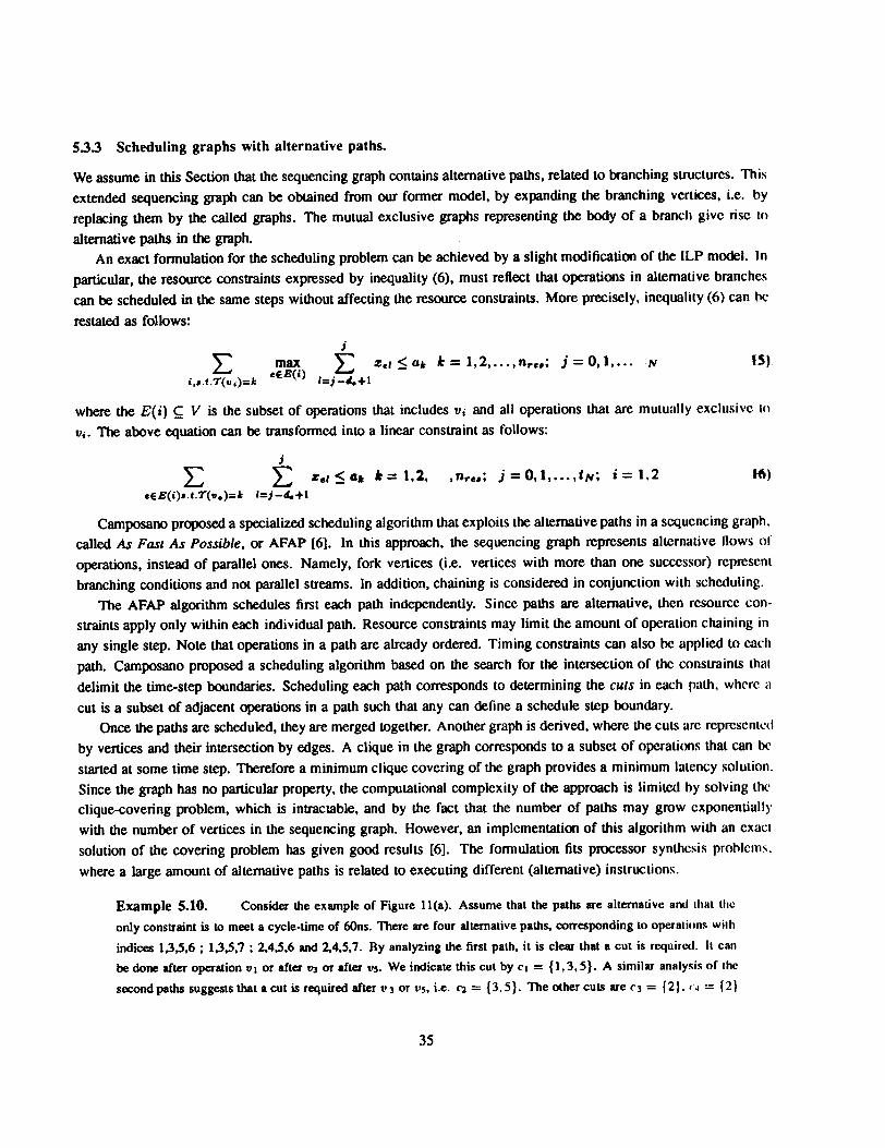
5.3.3 Scheduling graphs with alternative paths.

We assume in this Section that the sequencing graph contains alternative paths, related to branching struclures. Thisextended sequencing graph can be obtained from our former model, by ex~nding the branching vertices, i.e. byreplacing them by the called graphs. The mutual exclusive graphs representing the body of a branch give rise to

alternative paths in the graph.An exact formulation for the scheduling problem can be achieved by a slight modification of the ILP model. In

particular, the resource consb'aints expressed by inequality (6), musl reflect that operations in alternative branchescan be scheduled in the same steps wilhout affecting the resource constraints. More precisely, incqualily (6) can bc

restated as follows:

j

max EeEE(i) I=j -4.+1L

i...t.T(tI;)=k

1~)r.el~ak k=l,2,...,nr..; j=O,l,... N

where the E(i) ~ V is the subset of operations that includes Vi and all operations that are mutually exclllsivc 10

Vi. The above equation can be transformed into a linear constraint as follows:

j

}:::: }::::eEE(i)..t.T(v.)=J: I=j -4.+1

,nr.,; j=O.l,...,tN; i= 1,2 Iftc.~., s Ok, ,= 1.2.

Camposano proposed a specialized scheduling algorithm that exploits the alternative paths in a sequencing graph.called As Fast As Possible, or AFAP [6]. In this approach, the sequencing graph represents alternative Ilows or

operations, instead of parallel ones. Namely, fork vertices (i.e. vertices with more than one successor) representbranching conditions and not parallel streams. In addition, chaining is considered in conjunction with scheduling.

The AFAP algorithm schedules first each path independently. Since paths are alternative, then resource con-straints apply only within each individual path. Resource constraints may limit the amount of operation chaining inany single step. Note that operations in a path are already ordered. Timing constraints can also be applied to eachpath. Carnposano proposed a scheduling algorithm based on the search for the intersection of the constraints thatdelimit the time-step boundaries. Scheduling each path corresponds to determining the cuts in each path, where ,I

cut is a subset of adjacent operations in a path such that any can define a schedule step boundary.Once the paths are scheduled, they are merged together. Another graph is derived, where the cuts are represcntcd

by vertices and their intersection by edges. A clique in the graph corresponds to a subset of operations that can OC'

started at some time step. Therefore a minimum clique covering of the graph provides a minimum latency solution.Since the graph has no particular property, the computational complexity of the approach is limitc<1 by solving th(,clique-covering problem, which is intractable, and by the fact that the number of paths may grow exponentiallywith the number of vertices in the sequencing graph. However, an implementation of this algorithm with an exact

solution of the covering problem has given good results [6]. The formulation fits processor synthcsis prohlcms.where a large amount of alternative paths is related to executing different (alternative) instructions.

Example 5.10. Consider the example of Figure 11 (a). Assume that the paths are alternative an<I Ihal lhc

only constraint is to meet a cycle-lime of 6Ons. There are four alternative paths, corresponding to operalinn!O willI

indices 1,3,5,6 ; 1,3,5,7; 2,4,5,6 and 2,4,5,7. By analyzing the first path, it is clear that a cut is requirC(l. Il can

be done afler operation VI or afta'1/] or afta' vs. We indicate this cut by CI = {I, 3, 5}. A similar analy"i~ of the

socond paths suggests that a cut is r~uired afler l' 3 or vs, i.e. C2 = {3. 5}. The other cuts are ("3 = {21. '" = {21

35

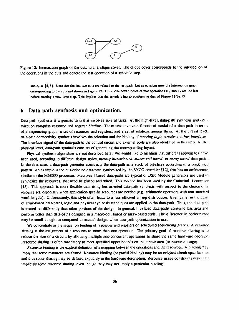
Figure 12: Intersection graph of d1e cuts wid1 a clique cover. The clique cover corresponds to the intersection or

d1e operations in d1e cuts and denote the last operation of a schedule step.

and c, = {4, 5}. Note that the last two cuts are related to the last path. let us consider now the intersecti()n graph

corresponding to the cuts and shown in Figure 12. The clique cover indicates that operations v 2 and I', arc the III~t

before starting a new time step. This implies that the schedule has to conform to that of Figure 11 (b). 0

Data-path synthesis and optimization.6

Data-path synthesis is a generic term that involves several tasks. At the high-level, data-path synthesis and opli-mization comprise resource and register binding. These task involve a functional model of a data-path in termsof a sequencing graph, a set of resources and registers, and a set of relations among them. At the circuit level.data-path connectivity synthesis involves the selection and the binding of steering logic circuits and bus interface.\".The interface signal of the data-path to the control circuit and external ports are also identified in thi~ ~tcp. Attht'

physical level, data-path synthesis consists of generating the corresponding layoutPhysical synthesis algorithms are not described here. We would like to mention that different approaches hayr

been used, according to different design styles, namely bus-oriented, macro-cell based, or array-ba.~ed data-paths.In the first case, a data-path generator constructs the data-path as a stack of bit-slices according to a predefincdpattern. An example is the bus-oriented data-path synthesized by the SYCO compiler [12], that has an architecturrsimilar to the M68CKX> processor. Macro-cell based data-paths are typical of DSP. Module generators are used tosynthesize the resources, that need be placed and wired. This method has been used by the Cathedral-II compiler[15]. This app-oach is more flexible than using bus-oriented data-path synthesis with respect to the choice of aresource set, especially when application-specific resources are needed (e.g. arithmetic operators with non-standardword lengths). Unfortunately, this style often leads to a less efficient wiring distribution. Eventually, in the ca~rof array-based data-paths, logic and physical synthesis techniques are applied to the data-path. Thus, the data-pathis treated no differently than other portions of the design. In g~neral, bit-sliced data-paths consume less arca andperform better than data-paths designed in a macro-cell based or array-based style. The difference in pcrfc)fmam't'may be small though, as compared to manual design, when data-path optimization is used.

We concentrate in the sequel on binding of resources and registers on scheduled sequencing graphs. A re.\"ourcesharing is the assignment of a resource to more than one operation. The primary goal of resource sharing is lOreduce the size of a circuit. by allowing multiple non-concurrent operations to share the same hardware operator.Resource sharing is often mandatory to meet specified upper bounds on the circuit area (or resource usage).

Resource binding is the explicit definition of a mapping ootween the o~rations and the resources. A binding may

imply that some resources are shared. Resource binding (or partial binding) may be an original circuit specificationand thus some sharing may be defined explicitly in the hardware description. Resource usage conSlrdinl.S may inrcr

implicitly some resource sharing, even though they may not imply a particular binding.

36

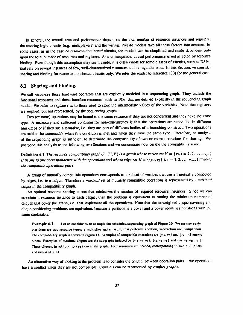
In general, the overall area and performance depend on the total number of resource instances and registers.the steering logic circuits (e.g. multiplexers) and the wiring. Precise models take all these factors into account. Insome cases, as in the case of resource-dominated circuits, the models can be simplified and made dependent onlyupon the total number of resources and registers. As a consequence, circuit performance is not affected by resourcebinding. Even though this assumption may seem crude, il is often viable for some classes of circuits, such as DSPs.that rely on several instances of few, well-characterized resources and storage elements. In this Section, ve considersharing and binding for resource-dominated circuits only. We refer the reader to reference [30] for lhe general cas('..

6.1 Sharing and binding.

We call resources mose hardware operators that are explicitly modeled in a sequencing graph. They include thefunctional resources and mose interface resources, such as vas, mat are defined explicitly in me sequencing graphmodel. We refer to registers as to mose used to store me intermediate values of the variables. NolC that regist('rsare implied, but not represented, by the sequencing graphs. .

Two (or more) operations may be bound to the same resource if they are not concurrent and they havc the saml.type. A necessary and sufficient condition for non-concurrency is that the operations are schedulcd in differenttime-steps or if they are alternative, i.e. they are part of different bodies of a branching construct. Two operationsare said to be compatible when this condition is met and when they have the same type. Thereforc, an analysisof the sequencing graph is sufficient to detennine thc compatibility of two or more operations for sharing. Wl'postpone this analysis to the following two Sections and we concentrate now on the the compatibility issu('.

1.2. ... .n",..!" ..r.} denole.Ii

Definition 6.1 The resource compatibility graph G +(\', E) is a graph whose vertex set V = {vs,; =is in one to one correspondence with the operations and whose edge set E = {{Vi, Vi} i, j = 1,2 the compatible operations pairs.

A group of mutually compatible operations corresponds to a subset of vertices that are all mutually connectedby edges, i.e. to a clique. Therefore a maximal set of mutually compatible operations is represented hy a maximlll

clique in the compatibility graph.An optimal resource sharing is one that minimizes the number of required resource instances. Since we can

associate a resource instJmce to each clique, than the problem is equivalent to finding the minimum number ofcliques that cover the graph, i.e. that implement all the operations. Note that the unweighted clique covering amiclique partitioning problems are equivalent, because a partitioo is a cover and a cover identifies partitions with th\..

same cardinality.

Example 6.1. Let us consider as an example the scheduled sequencing graph of Figure 10. We a55umc again

that there are two resource~: a multiplier and an ALU, that performs addiuon. subtraction and coolpari5()n.

The compatibility graph is shown in Figure 13. Examples of compatible operauons are {11 I. 113} and {"4. "51 among

others. Examples of maximal cliques are the subgraphs induced by {v I. 1'3. 1'7}. {1'1, 116,1"} and {114. "~. ".0. 1'111.

These cliques. in addiuon to {tl9} cover the graph. Four resources are needed. corresponding to two mlillipliers

and two ALUs. 0

An alternative way of looking at the problem is to consider the conflict between operation pairs. Two operation

have a conflict when they are not compatible. Conflicts can be represented by conflict graphs.

37

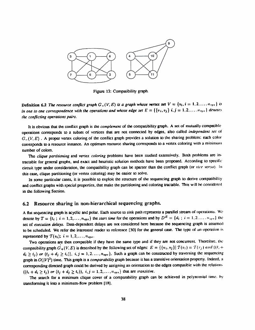
Figure 13: Compatibility graph.

Definition 6.2 The resource conflict graph G - (V, E) is a graph whose vertex set V = {tli' i = 1. 2. . . . . """,} i.{in one to one correspondence with the operation.\" and whose edge set E = {{ tl i, vi} i, j = 1.2,...; " "I"'} den(Jtr.\

the conflicting operations pairs.

It is obvious that the conflict graph is the complement of the compatibility graph. A set of mutually compatiblcoperations corresponds to a subset of vertices that are not connected by edges, also called independent .\'et or

G_(V, E) . A proper vertex coloring of the conflict graph provides a solution to the sharing problem: each colorcorresponds to a resource instance. An optimum resource sharing corresponds to a vertex coloring wilh a minimum

number of colors.The clique partitioning and vertex coloring problems have been studied extensively. Both problems arc in-

tIactable for general graphs, and exact and heuristic solution methods have been proposed. According to specificcircuit type under consideration, the compatibility graph can be sparser than the conflict graph (or ~'i(:e Ver.~(l). In

this case, clique partitioning (or vertex coloring) may be easier to solve.In some particular cases, it is possible to exploit the structure of the sequencing graph to derive compatibility

and conflict graphs with special properties, that make the partitioning and coloring tractable. This will he considered

in the following Section.

Resource sharing in non-hierarchical sequencing graphs.6.2

A flat sequencing graph is acyclic and polar. Each source to sink path represents a parallel stream of ollCralions. WI.'

denote by T = {ti ; i = 1,2, ...,nop,} the start time for the operations and by DE = {di ; i = 1.2 "o/',} lhc

set of execution delays. Data-dependent delays are not considered here because the sequencing graph is assuffiC<1to be scheduled. We refer the interested reader LO reference [30] for the general case. Thc lypc of ~In opcrali(m i~

represented by T(Vi); i = 1,2,..., nop$'

Two operations are then com~uble if they have the same type and if they are not concurrenl. Thcrcforc. lhc,

compatibility graph G +(V, E) is described by the following set of edges: E = {{Vi, Vj}1 T( Vi) = T( 'OJ) a"d (( f i +di ?: tj) or (tj + dj ?: ti»), i, j = 1,2 , nop.}. Such a graph can be constructed by traversing the sequencinggraph in O(IVI2) time. This graph is a comparability graph because it has a transitive orientation property. Indeed. ,Icorresponding directed graph could be derived by assigning an orientation to the edges compatible with the relalion~

«ti + di?: tj) or (tj +dj?: ti)), i,j = 1,2,...,nop,,} that are transitive.The search for a minimum clique cover of a comparability graph can be achieved in polynomial lim(',. hy

transforming it into a minimum-flow problem [18].

38

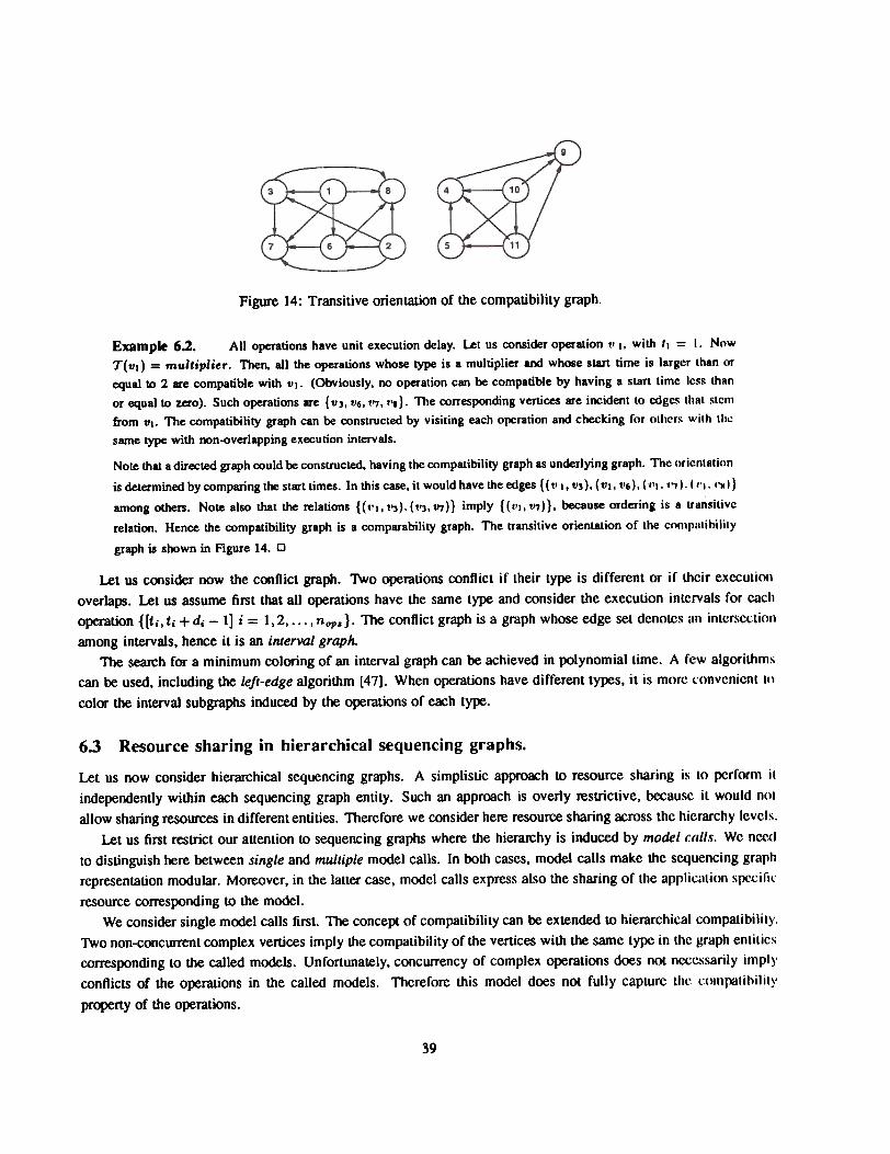
Figure 14: Transitive orientation of the compatibility graph.

Example 6.2. All operations have unit execution delay. Let us consider operation VI, with 11 = I. Now

T( VI) = multiplier. Then. all the operations whose type is a multiplier and whose sWt time is larger than orequal to 2 are compatible with VI. (Obviously. no operation can be compatible by having a start time le~~ than

or equal to zero). Such operations are {"3, "6,1'7, 1'1}. The corresponding venices are incident lo edg~ lhal stemfrom VI. The compatibility graph can be constructed by visiling each operation and checking for olhcr!' wilh lhe

same type with non-overlapping execution interVals.

Note that a directed graph could be constructed. having thc compatibility graph as underlying graph. The oricnlation

is determined by comparing the start times. In this case, it would have the edges {( VI, V3), (VI, tI6), (VI, 1'7). ( 1'1. I'M I}

among others. Note also that the relations {(t'I,t'3).(t'3,fJ7)} imply {(111,fJ7)}, because ordering is a transilive

relation. Hence the compatibility graph is a comparability graph. The transitive orientation of the compalihililY

graph is shown in Figure 14. 0

Let us consider now the conflict graph. Two operations conflict if their type is different or if their executionoverlaps. Let us assume first that all operations have the same type and consider the execution intervals for eachoperation {[t" t, + d, - 1] i = 1,2,..., nop. }. The conflict graph is a graph whose edge set denotes an intersection

among intervals, hence it is an interval graph.The search for a minimum coloring of an interval graph can be achieved in polynomial time. A few algorithms

can be used, including the left-edge algorithm [47]. When operations have different ty~s, it is more convenicnl!.!)

color the interval subgraphs induced by the o~rations of each ty~.

Resource sharing in hierarchical sequencing graphs.6.3

Let us now consider hierarchical sequencing graphs. A simplistic approach to resource sharing is LO pcrform iLindependently within each sequencing graph entity. Such an approach is overly restrictive, becausc il would nOIallow sharing resources in different entities. Therefore we consider here resource sharing across lhe hierarchy levcls.

Let us first restrict our atlention to sequencing graphs where the hieran:hy is induced by model call.\". We ncc{1

lO distinguish here between single and multiple model calls. In both cases, model caIJs make the sequencing graphrepresentation modular. Moreover, in the latter case, model caIJs express also the sharing of the applic~llion spccifi.

resource corresponding to the model.We consider single model calls first. The concept of compatibility can 00 extended to hierarchical compatibiliLy.

Two non-concurrent complex vertices imply the compatibility of the vertices with the same lype in the graph enlitiescorresponding to the called models. Unfortunately, concurrency of complex operations does not nccc.'isarily implyconflicts of the operations in the called models. Therefore this model does not fully caplure lhr l:ompalihilily

property of the operations.

39

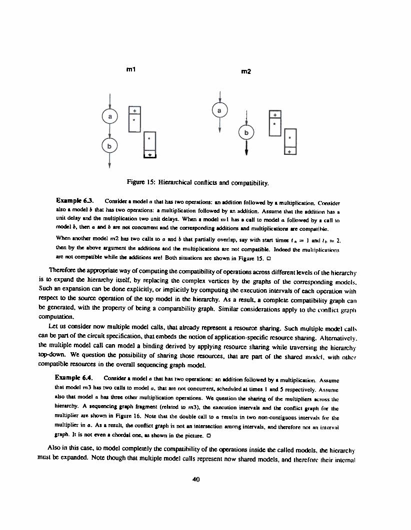
m1 m2

~

L..t.J

Figure 15: HierarchicaJ conflicts and com.-tibility.

Example 6.3. Consider a model a that has two operations: an addition followed by a multiplication. Considl..'Talso a model b that has two operations: a multiplication followed by an addition. Assume that the addili()n has Hunit delay and the multiplication two unit delays. When a model nJ I has a call to model a followed by a call 10

model b. then a and b are not concurrent and the correspoooing additions and multiplications are compalihle..

When another model m2 has two calls to a and b that partially overlap. say with start times t Q = I and I,. = 2.

then by the above argument the additions and the multiplications are nol compatible. Indeed the mullirlicalion~

are not compatible while the ackIitions arel Both situations are shown in Figure 15. 0

Theref(X'e the appropriate way of compuung the compaubility of operauons across different levels of the hierdfchyis to expand the hierarchy itself, by replacing the complex vertices by the graphs of the corresponding modcls.Such an expansion can be done explicitly, or implicitly by computing the execution intervals of each operation withrespect to the source operation of the top model in tre hierarchy. As a result. a complete compatibility graph canbe generated, with the property of being a comparability graph. Similar considerations apply to the 1:()f1ni(~l graph

computauon.Let us consider now multiple model calls, that alrcady rep-esent a resource sharing. Such multiplc mO<kl call~

can be part of the circuit specificauon, that embeds the nouon of application-s~ific resource sharing. A Itcmativcly.the multiple model call can model a binding derived by applying resource sharing while traversing the hierarchy

~own. We question the possibility of sharing those resources, that are part of the shared m()(ll~I, with olhl'rcompatible resources in the overall sequencing graph model.

Example 6.4. Consider a model a that has two operations: an addition followed by a multiplicaticJn. AssunlC

that model m3 has two calls to model a, that are not concurrent. scheduled at times I and 5 respectively. AssunlC

also that model a has three other multiplication operations. We question Lhe sharing of the multipliers across tllC

hieruchy. A sequencing grlph fragment (related to m3). the ex«:ution intervals and the conflict graph for thc

multiplier are soown in Figure 16. Note that the double call to a results in two non-<:ontiguous interval!' rOT tile

multiplier in a. As a result. Lhe conflict graph is not an intersection among intervals. and thererore nm an intL'fVltl

graph. It is not even a ctmdal one. as shown in the picture. 0

Also in this case, to model completely the compatibility of the operations inside the called models, the hierarchymust re expanded. Note though that multiple model calls represent now shared models, and lhererorr lhcir intcmal

40

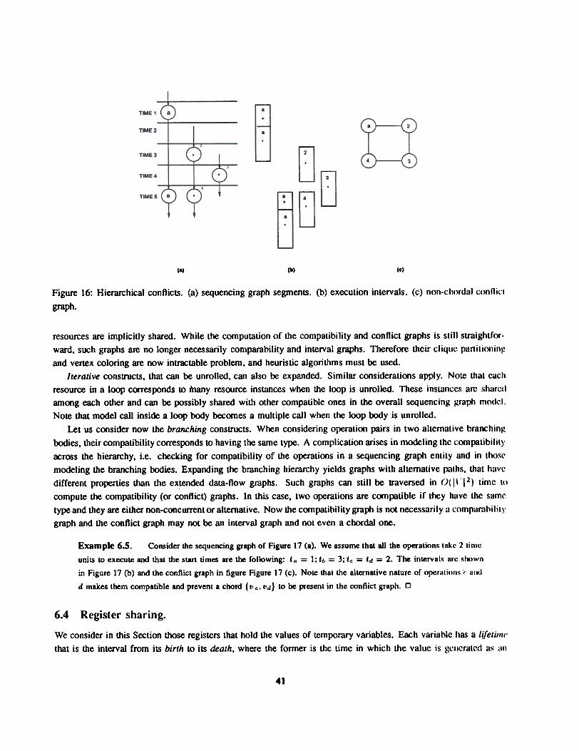
C-I (0)(8)

Figure 16: Hierarchical conflic~. (a) sequencing graph segmen~. (b) execution intervals. (c) non-chordal conl1irl

graph.

resources are implicitly shared. While the computation of the compatibility and conflict graphs is slill straightfor-ward, such graphs are no longer necessarily comparability and interval graphs. Therefore their clique partilioningand vertex coloring are now intractable problem, and heuristic algorithms must be used.

Iterative conslructs, that can be unrolled, can also be expanded. Similar considerations apply. Note thal eachresource in a loop cOITesponds to many resource inSlances when the loop is unrolled. These inslanccs arc sharc(1among each other and can be possibly shared with other compatible ones in the overall sequencing graph mo<lcl.Note that model call inside a loop body becomes a multiple call when the loop body is unrolled.

Let us consider now the branching constructs. When considering operation pairs in two altemalive branchingbodies, their compatibility cOlTesponds to having the same type. A complication arises in modeling the compatibilityocross the hierarchy, i.e. checking for compatibility of the operations in a sequencing graph enlily and in tho$emodeling the branching bodies. Expanding the branching hierarchy yields graphs with alternative paLhs, thaL havedifferent properties than the extended dala-ftow graphs. Such graphs can still be traversed in O( I ~ '12) time l()

compute the compatibility (or conflict) graphs. In this case, two operations are compatible if they have the sametype and they are either non-concurrent or alternative. Now the compatibility graph is not necessarily a comp~lrnhilil ygraph and the conflict graph may not be an interval graph and not even a chordal one.

Example 6.S. Consider the sequencing graph of Figure 17 (a). We assume that all the operalions lakc 2 limc

units to execute and that the start limes are the following: t" = 1; t" = 3; tc = td = 2. The inlervals arc shown

in Figure 17 (b) and the conflict graph in figure Figure 17 (c). Note thallhe allernalive nature of operalicln!' ( and

d makes them compatible and prevenl a chord {tl c. t'd} lo be presenl in lhe conflict graph. 0

6.4 Register sharing.

We consider in this Section those registers that hold the values of temporary variables. Each variable has a /ifetiml'that is the interval from its birth to its death, where the former is the time in which the value is gc.llcrat('.d as (\II

~1

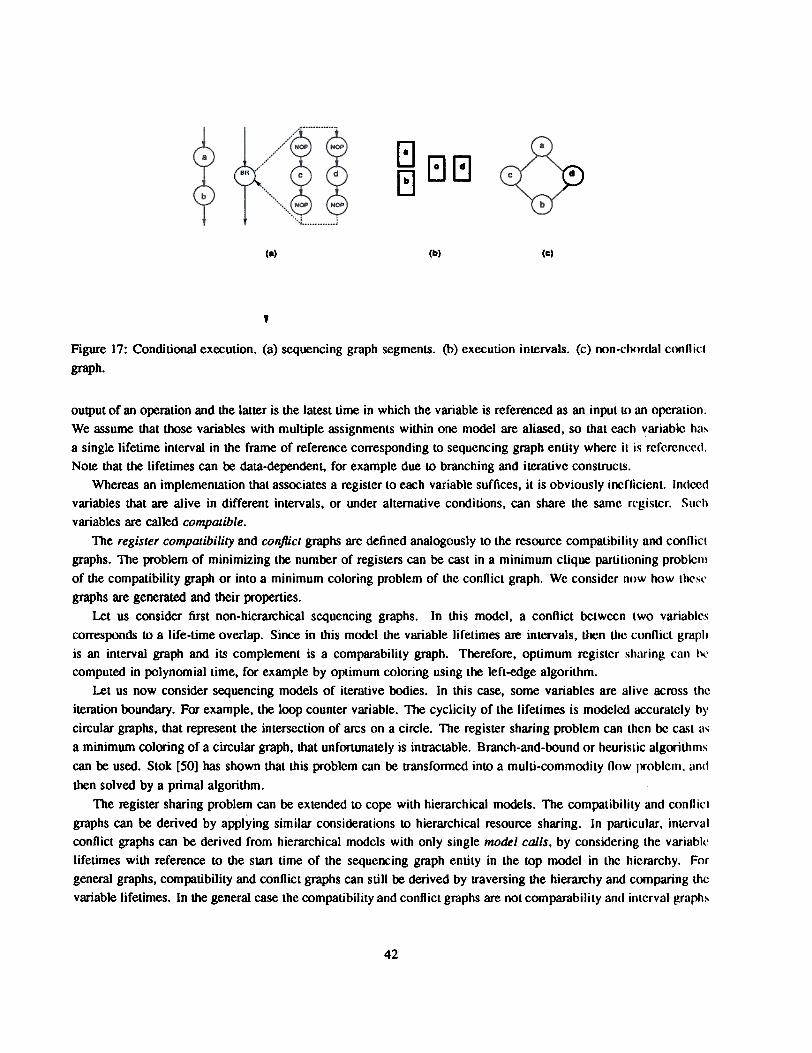
[:J

GSS ~(e) (b) (0)

,Figure 17: Conditional execution. (a) sequencing graph segments. (b) execution intervals. (c) non-chordal conllici

graph.

output of an operation and the latter is the latest time in which the variable is referenced as an input to an operation.We assume that those variables with multiple assignments within one model are aliased, so that each variablc hasa single lifetime interval in the frame of reference corresponding to sequencing graph entity where it is referenced.Note that the lifetimes can 00 data-dependent, for example due to branching and iterative construcL~.

Whereas an implementation that associates a register to each variable suffices, it is obviously inefficient. Indeedvariables that are alive in different intervals, or under alternative conditions, can share the same rl~gistcr. Suchvariables are called compatible.

The register compatibility and conflict graphs are defined analogously to the resource compalibility and conflictgraphs. The problem of minimizing the numoor of registers can be cast in a minimum clique parlilioning problemof the compatibility graph or into a minimum coloring problem of the conflict graph. We consider J1()W how tl~sl.graphs are generaled and their properties.

Let us consider first non-hierarchical sequencing graphs. In this model, a confticl bclwccn two variablescorresponds to a life-time overlap. Since in this model Lhe variable lifetimes are inlervals, lhen Lhc cunnict graphis an interval graph and its complement is a comparabilily graph. Therefore, optimum register sharing c~ln I'l'compuled in polynomial time, for example by oplimum coloring using lhe lefl-edge algorilhm.

Let us now consider sequencing models of iteralive bodies. In this case, some variables are alive across theiteration boundary. For example, lhe loop counter variable. The cyclicily of the lifelimes is modeled accuralely bycircular graphs, that represent the intersection of arcs on a circle. The register sharing problem can then bc ca.~t a,a minimum coloring of a circular graph, that unfortunately is intractable. Branch-and-round or heuristic algoriLhmscan 00 used. Stok [50] has shown that Lhis problem can 00 transformed into a multi-commodily now problem. amithen solved by a primal algorithm.

The register sharing problem can be extended lO cope willi hierarchical models. The compalibility and conl1ictgraphs can be derived by applying similar consideralions to hierarchical resource sharing. In particular, intervalconflict graphs can be derived from hierarchical models with only single model calls, by considering lhe variabll~lifetimes with reference to the start time of the sequencing graph entilY in lhe top model in Lhc hicmrchy. Forgeneral graphs, compatibility and conflicl graphs can still 00 derived by lfaversing the hierarchy and comparing Lhcvariable lifetimes. In Lhe general case the compatibility and conflict gmphs are not comparability and interval !,rraphs

42

respectively, and therefore the corresponding optimal register sharing problem is intractable. Springer and Thomas[49] have shown that polynomial-time colorable conflict graphs can be achieved by enforcing some restrictions 011

the model calls and on the branch types.

6.5 Other binding and sharing problems.

Other binding and sharing problems stem from the use of particular circuits, soch as memory arrays. busses, ami

interfaces.Some design styles use multi-port memories to store the values of the variables. Such memories are also referrc<1

to as general-purpose registers (GPRs), common to RISC architectures. Let us assume the memory has a portsfor either read and write requiring one cycle per access. A binding problem consists of computing the minimumnumber of ports a required to occess as many variables as needed. Balakrishnan et alii [2] considered the dualproblem. They assumed a fixed number of ports and they maximized the number of variables to bc stored in thl.'multi-port memory, subject to the port limitation. Both problems can be rormulated as lLPs.

Busses act as transfer resources that feed data to functional resources. The o~ration or writing a specific bus callbe modeled explicitly as a vertex in the sequencing graph model. In this case, the compatible (or connicting) daUItransfers may be modeled by com~tibility (or connict) graphs, as in the case of functional resources. Alternatively.busses may not be explicitly described in the sequencing graph model. Their (optimal) usage can be then dcrivc<1by exploiting the data trarlSfers. Since busses have no memory, we consider only the transfers or daUi within eachschedule step (or across two adjacent schedule steps, when we assume lhatthe bus transfer is inLerleavcd with lhl'computation). Two problems then arise. First, to find the minimum number of busses to accommodate all (or partof) the data transfers. Second, find the maximum number of data transrers that can be done through a ~iven nllmb<.'rof busses. Both problems can be modeled again by ILPs.

Control synthesis.7

We consider in this Section the synthesis of the control units. From a circuit implementation poinl of view, wecan classify the control-unit model as microcode-based or hard-wired. The former implementalion stylc slOres th(,control information into a read-only memory (ROM) array, while the latter uses a hard-wired sequential circuitconsisting of an interconnection of a combinational circuit and registers. From a logic stand-point, synchronousimplementation of control can be modeled as a finite-state machine. Both implementation styles can bc modcledas such. because a read-only memory and a synchronous counter behave as a finite automalcm as well as aninterconnection of combinational logic gates and synchronous registers.

The interface betWeen the data-path and the control circuit is provided by the signals that enable lhe rcgislers,and that control the steering circuits (i.e. multiplexers and busses). Sequential resources require an activation(and sometimes a reset) signal. Data-dependent operations must provide a completion signals. The ensemblrof these control points are identified during the synthesis of the data-path. In addition, lhe control unit require.ssome condition signals from the data-path, thal are needed to evaluale the clauses of some branching and ilcralivl.'

constructs.

Example 7.1. Figure 18 shows an example of the interconneclion between the data-path and l'Ontrol.

The data-path provides signals to the control unit relaled to the execution of alternative control flows. ..uch liS

-43

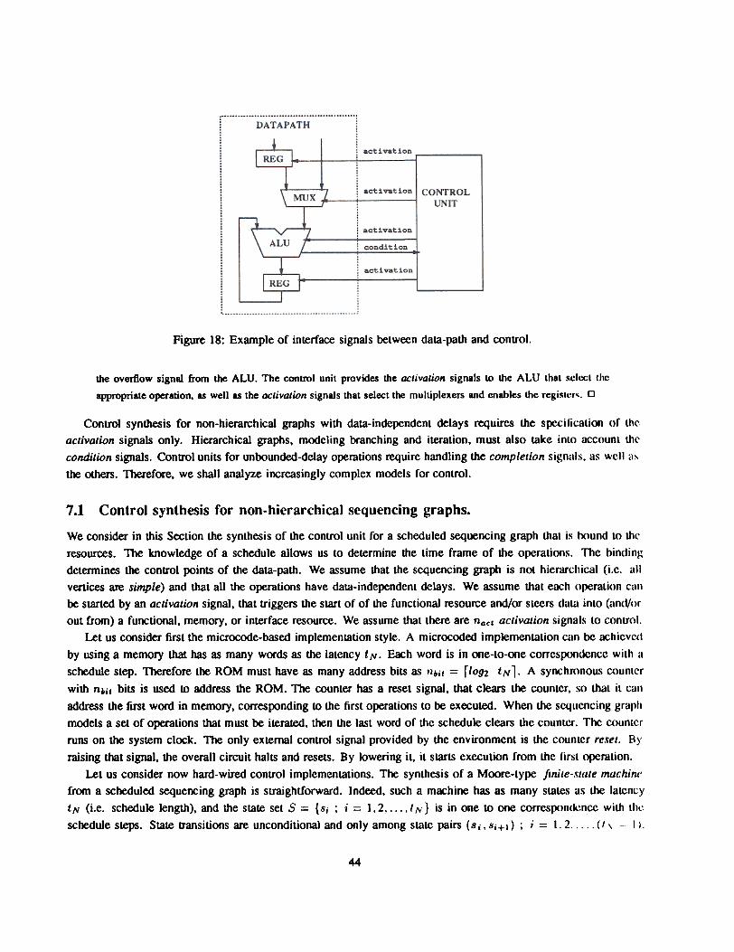
Figure 18: Example of interface signals between data-path and control.

the overflow signal from the ALU. The control unit provides the activation signals to the ALU that select the

appropriate operation. as well as the activation signals that select the multiplexers and enables the regi~tl'r". 0

Control synthesis for non-hieran:hical graphs with data-independent delays ~uires the s~cification of thractivation signals only. Hierarchical graphs, modeling branching and iteration, must also take into account th('condition signals. Control units for unbounded-delay operations ~uire handling the completion sigrulls. as wcll ,ISthe others. Therefore, we shall analyze increasingly complex models for control.

Control synthesis for non-hierarchical sequencing graphs.7.1We consider in this Section the synthesis of the control unit for a scheduled sequencing graph that is round to 1hrresources. The knowledge of a schedule allows us lO determine the time frame of the operations. The bindin~determines the conb"ol points of the data-path. We assume that the sequencing graph is not hierdrchical (i.e. allvertices are simple) and that all the operations have data-independent delays. We assume thal each opera1ion canbe started by an activation signal, that triggers the start of of the functional resource and/or Slccrs data inlo (an<Vorout from) a functional, memory, or interface resource. We assume tha1lhere are nact activalion signals lO C()ntrol.

Let us consider first the microcode-based implementation style. A microcoded implementalion cun be achicvc{!by using a memory that has as many words as the latency tN. Each word is in one-to-one correspondence wilh aschedule step. Therefore the ROM must have as many address bits as Ilbit = r/O92 tN 1. A synchronous COunlrr

with nbit bits is used to address the ROM. The counter has a reset signal, that clears the counter, so thal il can

address the first word in memory, corresponding to the first operations to be executed. When the sequencing graphmodels a set of operations that must be iterated, then the las1 word of the schedule clears the counter. The counLcrruns on the system clock. The only external control signal provided by the environment is the counter re.\"et. Byraising that signal, the overall circuit halts and resets. By lowering il, it starts execution from the first operation.

Let us consider now hard-wired control implementations. The synthesis of a Moore-type ftnile-.~lale machim~from a scheduled sequencing graph is straightforward. Indeed, such a machine has as many states as the latencytN (i.e. schedule length), and the state set S = {Sj ; i = 1,2,..., /. N} is in one to one correspondl..ncc with lhl'schedule steps. State b"ansitions are unconditional and only among Slate pairs (8 i, 8i+1) ; i = 1.2 (I \ - 1).

44

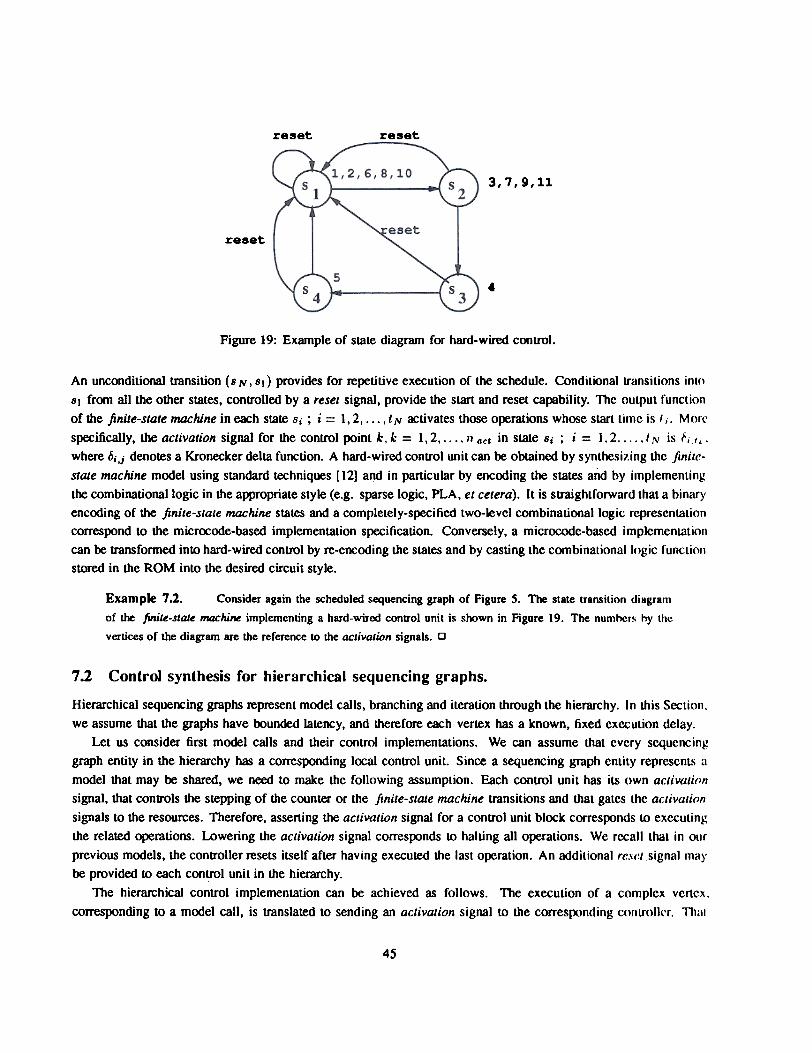
reset reset

3,7,9,11

reset

4

Figure 19: Example of stale diagram for hard-wired control.

An unconditional transition (8 N, 81) provides for repetitive execution of the schedule. Conditional transitions into81 from all the other states, controlled by a reset signal, provide the start and reset capability. The output functionof the finite-state machine in each state 8j ; i = 1,2,..., t N activates those operations whose start time is Ii. Morrspecifically, the activation signal for the control point k, k = 1,2,..., n lI.:t in state 8j ; i = 1.2 , Il\' is "i.t,.

where DjJ denotes a Kronecker delta function. A hard-wired control unit can be obtained by synthesizing the finite-state machine model using standard techniques [12] and in particular by encoding the states and by implementingthe combinational logic in the appropriate style (e.g. sparse logic, PLA, et cetera). It is straightforward that a binaryencoding of the finite-state machine states and a completely-specified two-level combinational logic representationcorrespond to the microcode-based implementation specification. Conversely, a microcode-based implementationcan be transformed into hard-wired control by re-encoding the states and by casting the combinational logic runctionstored in the ROM into the desired circuit style.

Example 7.2. Consider again the scheduled sequencing graph of Figure 5. The state transition diagram

of the finite-state machine implementing a hard-wired control unit is shown in Figure 19. The numhcrs j,y the

vertices of the diagram are the reference to the activation signals. 0

7.2 Control synthesis for hierarchical sequencing graphs.

Hierarchical sequencing graphs represent model calls, branching and iteration through the hierarchy. In this Section.we assume that the graphs have bounded latency, and therefore each vertex has a known, fixed execution delay.

Let us consider first model calls and their control implementations. We can assume that every sequencinggraph entity in the hierarchy has a corresponding local control unit. Since a sequencing graph entity represent'i amodel that may be shared, we need to make the following assumption. Each control unit has its own activationsignal, that conb'ols the stepping of the counter or the finite-state machine transitions and that gates the activationsignals to the resources. Therefore, asserting the activation signal for a conb'ol unit block corresponds to executingthe related operations. Lowering the activation signal corresponds to halting all operations. We recall that in ourprevious models, the conb'oller resets itself after having executed the last operation. An additional re.{(~t signal maybe provided to each control unit in the hierarchy.

The hierarchical control implementation can be achieved as follows. The execution of a complex vertcx.

corresponding to a model call, is translated to sending an activation signal to the corres(X>nding controllc!. Thai

45

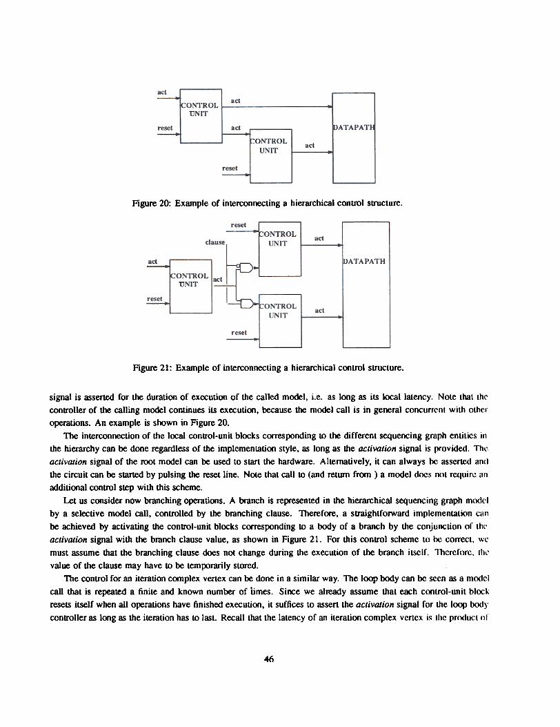
Figure 20: Example of interconnecting a hierarchical control Sb"uClure.

Figure 21: Example of interconnecting a hierarchical control structure.

signal is asserted for the duration of execution of the called model, i.e. as long as its local latency. Note that theconb'oller of the calling model continues its execution, oocause the model call is in general concurrent with otheroperations. An example is shown in Figure 20.

The interconnection of the local conb'Ol-unit blocks corresJX}nding to the different sequencing graph entities inthe hierarchy can 00 done regardless of the implementation style, as long as the activation signal is provided. Thcactivation signal of the root model can 00 used to start the hardware. Alternatively, it can always be asserted andthe circuit can 00 started by pulsing the reset line. Note that call to (and return from) a model docs not require alladditional control step with this scheme.

Let us consider now branching operations. A branch is represented in the hierarchical sequencing graph m<)(jelby a selective model call, controlled by the branching clause. Therefore, a sb'aightforward implementation CClIl00 achieved by activating the conb'Ol-unit blocks corresJX}nding to a body of a branch by the conjunction of thcactivation signal with the branch clause value, as shown in Figure 21. For this conb'Ol scheme to I)C correct, wcmust assume that the branching clause does not change during the execution of the branch itself. Therefore, 1 hI.'value of the clause may have to be temJX}rarily stored.

The control for an iteration complex vertex can be done in a similar way. The loop body can be seen as a modelcall that is repeated a finite and known number of urnes. Since we already assume that each control-unit blockresets itself when all operations have finished execution, it suffices to assert the activation signal for tt1e loop bodyconb'OlIer as long as the iteration has to last. Recall that the latency of an iteration complex vertex is the product or

46

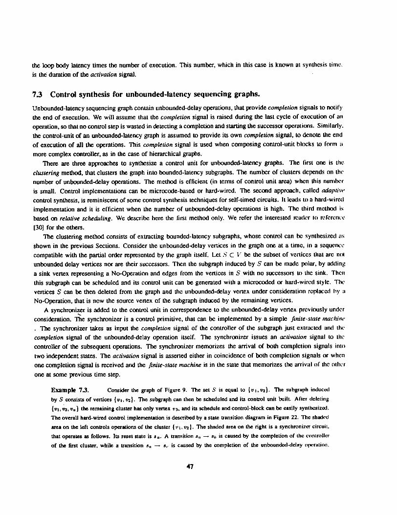
the loop OOdy latency times the number of execution. This number, which in this case is known at !iynthcsis time.

is the duration of the activation signal.

7.3 Control synthesis for unbounded-latency sequencing graphs.

Unbounded-latency sequencing graph contain unbounded-delay operations, that provide completion signals to nolifylhe end of execution. We will assume that lhe completion signal is raised during lhe lasl cycle of execution of an

operation, so that no control step is wasted in detecting a completion and starting lhe successor operalions. Similarly.lhe control-unit of an unbounded-latency graph is assumed to provide its own completion signal, to denote lhe endof execution of alilhe operations. This completion signal is used when composing control-unil bl()Cks to form il

more complex controller, as in the case of hierarchical graphs.There are three approaches to synthesize a control unil for unbounded-latency graphs. The firsl one is lhl.~

clustering melhod, that clusters lhe graph into bounded-latency subgraphs. The number of clusters depends on lhcnumber of unbounded-delay operations. The melhod is efficient (in terms of control unit area) when lhis numberis small. Control implementations can be microcode-based or hard-wired. The second approoch, called adaptiv('control synthesis, is reminiscent of some control synlhesis techniques for self-timed circuits. It leads lO a hard-wire<1implementation and it is efficient when lhe number of unbounded-delay operations is high. Thc lhird mcttKJd isbased on relative scheduling. We describe here lhe first melhod only. We refer lhe intereslCd rcad('r 10 rcfcrl~n,\.'

[30] for lhe olhers.The clustering melhod consists of extracting bounded-latency subgraphs, whose conlrOl can be synlhesi7.e<1 as

shown in lhe previous Sections. Consider lhe unbounded-delay vertices in lhe graph one al a lime, in a sequencecompatible wilh lhe partial order represented by lhe graph itself. Lel ,) C \" be lhe subset of vertices lhat are n()\unbounded delay vertices nor are lheir successors. Then lhe subgraph induced by S can be made polar, by oodinga sink vertex representing a No-Operation and edges from lhe vertices in S wilh no successors LO lhc sink. Thcnlhis subgraph can be scheduled and its conlrOl unil can be generated wilh a microcoded or hard-wired slylc. Th\.'vertices S can be lhen deleted from lhe graph and lhe unbounded-delay vertex under consideralion rcploce<1 hy aNo-Operation, lhat is now lhe source venex of lhe subgraph induced by lhe remaining vertices.

A synchronizer is added lO lhe control unit in correspondence La lhe unbounded-delay vertex previously under...

consideration. The synchronizer is a conlrol primitive, lhat can be implemenled by a simple finite-,~tate tnachin('. The synchronizer takes as input lhe completion signal of lhe controller of lhe subgraph jusl exlracted ami lh\.'completion signal of lhe unbounded-delay operalion itself. The synchroni7.er issues an activation signal lo lh('controller of the subsequent operations. The synchroni7.er memorizes lhe arrival of bolh complclion signals intI)two independent states. The activation signal is asserted eilher in coincidence of bolh completion signals or whe.1lone completion signal is received and lhe ftnite-.~tate machine is in me state lhat memorizes lhe arrivill of lI1e other

one at some previous lime step.

Example 7.3. Consider the graph of Figure 9. The set S is equal to {VI,V2}. The subgraph inducC(1

by S oonsists of vertices {VI, V2}. The subgraph can then 00 scheduled and its oonl1Ol unit builL Afler dcleling

{VI'~' va} the remaining cluster has only vertex t/3, and its schedule and control-block can be easily synlhcsizcd.

The overall hard-wired oonlrol implementation is described by a state Iransition diagram in Figure 22. The shaded

area on the left conlrols operations of the cluster {(II. t'2}. The shaded area on the right is a synchroni7.er circuil.

that operates as follows. Its reset state is So. A transition So - Sb is caused by the completion of the I.'()nlroller

of the first cluster, while a transition So - s,. is caused by the oompletion of the unbounded-dclay ()!1l,raliol1.

47

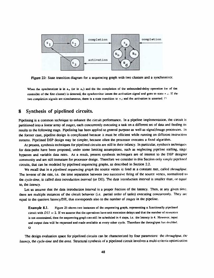
Figure 22: State transition diagram for a sequencing graph with two clusters and a synchronizer.

When the synchroniza- is in Sa (or in sc) and the the completion of the unbounded-deJay operation «If or the

controller of the first cluster) is detected, the synchronizer issues the activation signal and goes 10 stalc OJ ./. If lh<'

two completion signals are simultaneous, there is a slate transition 10 .S d and the activation is asserlcd. rl

Synthesis of pipelined circuits.8

Pipelining is a common technique to enhance the circuit ~rformance. In a pipeline implementation, lhe circuil ispartitioned into a linear array of stages, each concurrently executing a lask on a different set of data and feeding iL..results to the following stage. Pipelining has been applied to general purpose as well as signal/image processors. Inthe former case, pipe\ine design is complicated because it must be efficient while running on diffcrcnl inSlrUCliol1Sb'eamS. Pipelined DSP design may be simpler, because often the processor executes a fixed algorithm.

At present. synthesis techniques for pipelined circuits are still in their infancy. In particular, synthcsis lechniqucsfor data-paths have been proposed, under some limiting assumptions, such as neglecting pi~line slalling, stagcbypasses and variable data rates. As a result. present synthesis lechniques are of inlerest lo the DSP designercommunity and are still imrnalure for processor design. Therefore we consider in this Seclion only simple pipclinc{1circuits, that can be modeled by pipelined sequencing graphs, as described in Section 2.2.

We recall that in a pipelined sequencing graph thc source vertex is fired at a constant rate, callcd throughput.The inverse of the rate, i.e. the time separation between two successive firing of the source verLCx, normali7.ed tothe cycle-time, is called data introduction interval (or DII). The data inlroduction interval is smallcr Ihan, (Ir Cl.JllilJ

to, the latency.Let us assume that the data introduction interval is a proper fraclion of the latency. Then, at any givcn time.

there are multiple instances of the circuit behavior (i.e. partial order of tasks) executing concurrcnlly. Thcy art'equal lo the quotient latencyfDII, that corresponds also lo the number of stages in the pi~line.

Example 8.1. Figure 23 shows two instances of the sequencing graph. representing a functionally pipclincd

circuit with D I I = 2. If we assume that the operations have unit execution delays arKi that the number of resources

is not constrained. then the sequencing graph can still be scheduled in 4 steps, i.e. the latency is 4. However. input

arKi output data will be requested and made available at every other cycle. Therefore the throughput hll!; Ik1Uhleil.

0

The design evaluation space for pipelined circuits can be characterized by four parameters: lhe throughput. lhe

latency, lhe cycle-time and lhe area. Structural synthesis of a pipelined circuit involves a multi-criteria oplimi"..1liOil

48

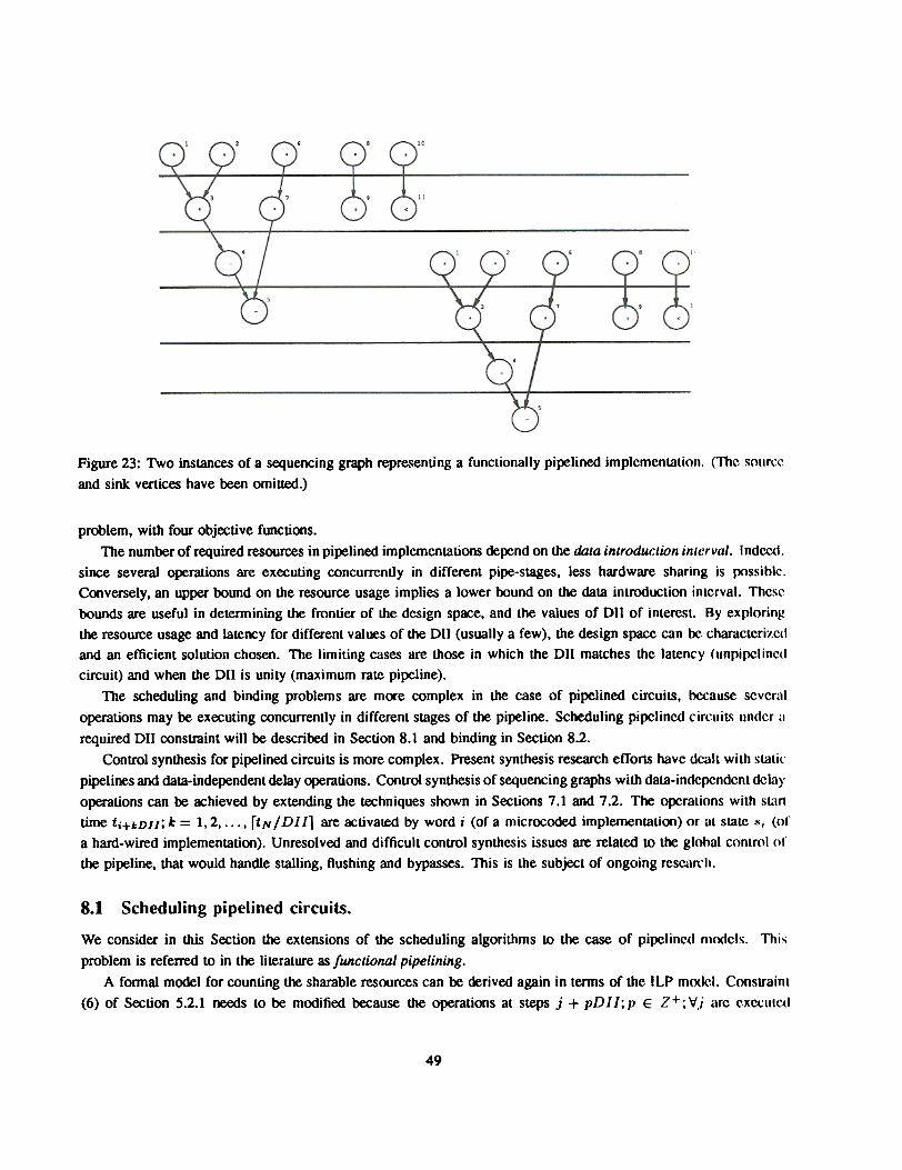
Figure 23: Two instances of a sequencing graph representing a functionally pipelined implcmentaLion. (The !iOllrC('

and sink vertices have been omitted.)

problem, with four objective functions.The number of required resources in pipelined implementations de~nd on the data introduction interval. Indcc<l.

since several o~rations are executing concurrently in different pipe-stages, less hardware sharing is possible.Conversely, an upper bound on the resource usage implies a lower bound on the data introduction interval. Thesebounds are useful in determining the frontier of the design space, and the values of 011 of intere...t. By exploringthe resouree usage and latency for different values of the 011 (usually a few), the design space can be characterii'.c<1and an efficient solution chosen. The limiting cases are those in which the 011 matches the latency (unpipclinc<1circuit) and when the 011 is unity (maximum rate pipeline).

The scheduling and binding problems are more complex in the case of pipelined circuits, because scvcr.11operations may be executing concurrently in different stages of the pipeline. Scheduling pipclined circuil~ under .1required 011 constraint will be described in Section 8.1 and binding in Section 8.2.

Control synthesis for pipelined circuits is more complex. Present synthesis research efforts have dealt with staticpipelines and data-independent delay operations. Control synthesis of sequencing graphs with data-independent delayoperations can be IK:hieved by extending the techniques shown in Sections 7.1 and 7.2. The operations with st.1ntime ti+kDll;k = 1,2,..., rtN/DIJl are IK:tivated by word i (of a microcoded implementation) or at Slate .~; (ora hard-wired implementation). Unresolved and difficult control synthesis issues are related to the global control ofthe pipeline, that would handle slatling, flushing and bypasses. This is the subject of ongoing res~I~II.

Scheduling pipelined circuits.8.1

We consider in dlis Section the extensions of die scheduling algorithms to the case of pipelinccl mc)c:jcls. This

problem is referred to in die literature as functional pipelining.A formal model for counting the sharable resources can be derived again in terms of die ILP moclcl. Constrainl

(6) of Section 5.2.1 needs to be modified because die operations at steps j + pD I I; p E Z +; '1/.; arc c.xCCIlIC~1

49

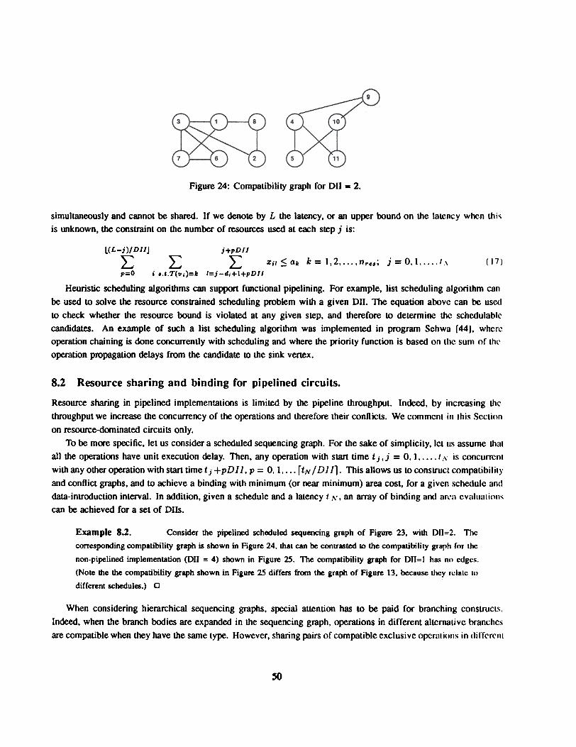
Figure 24: Compatibility graph for 011 = 2.

simultaneously and cannot be shared. If we denote by L the latency, or an upper bound on the latency wh('.n thisis unknown, the constraint on the number of resoU1t:es used at eoch step j is:

l(L-j)/DIIJ j+pD/I

L L L Zil$ak k=1,2,...,nre.: j=O.l /, (17)p=o i ..t.T(tI;)=k l=j-d;+I+pD/l

Heuristic scheduling algorid1ms can support functional pipelining. For example, list scheduling algorithm canbe used to solve the resource constrained scheduling problem wid1 a given 011. The equation aoovc can be use<1to check whether d1e resource bound is violated at any given step, and d1erefore 10 determine d1c schedulablccandidates. An example of such a list scheduling algorid1m was implemented in program Schwa [44], whereoperation chaining is done concurrently with scheduling and where d1e priority function is based on Lhc sum of Lhroperation propagation delays from d1e candidate 10 d1c sink vertex.

8.2 Resource sharing and binding for pipelined circuits.

Resource sharing in pipelined implementations is limited by the pipeline throughput. InOOed, by increasing thethroughput we increase the concurrency of the operations and therefore their conflicts. We comment in this Sectionon resource-dominated circuits only.

To be more specific. let us consider a scheduled sequencing graph. For the sake of simplicity, let us assume thatall the operations have unit execution delay. Then. any operation with start time t j ,j = O. 1. . . . . / i'" is concurrcnlwith any other operation with start time tj +pDII, p = 0.1,... rtN IDI fl. This allows us to construct compatibilityand conflict graphs, and to achieve a binding with minimum (or near minimum) area cost. for a given scheclule amidata-introduction interval. In addition. given a schedule and a latency f N, an array of binding ami 3rl'a evalU31iol1scan be achieved for a set of DIIs.

Example 8.2. Consider the pipelined scheduled sequencing graph of Figure 23, with 00=2. The

correspoooing compatibility graph is shown in Figure 24. that can be contrasted to the compatibility graph for the

non-pipelined implementation (00 = 4) shown in Figure 25. The compatibility graph for 011=1 ha.~ rnl edges.

(Note the the compatibility graph shown in Figure 25 differs from the graph of Figure 13, because they rclale 10

different schedules.) 0

When considering hierarchical sequencing graphs, special attention has to be paid for branching construct".Indeed, when the branch bodies are expanded in the sequencing graph, operations in different altcrnalive branchesare compatible when they have the same type. However, sharing pairs of compatible exclusive operaliOlls in (Iirrcrcnl

so

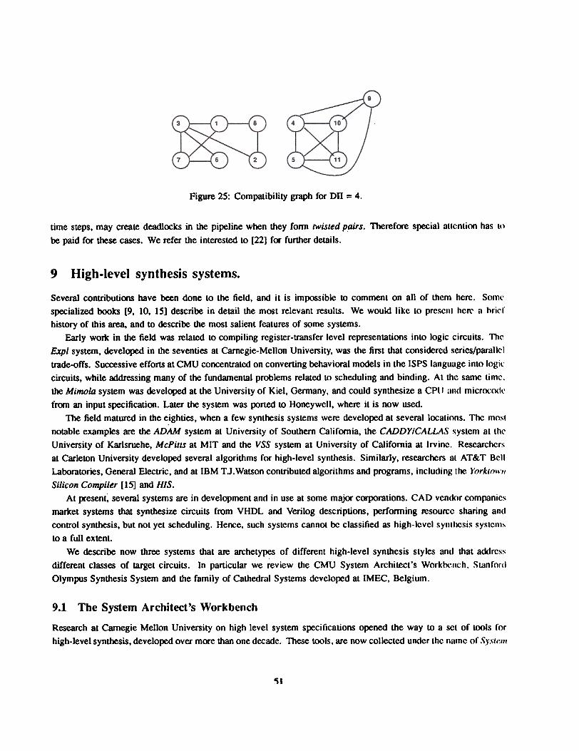
Figure 25: Compatibility graph for Dll = 4.

time steps. may create deadlocks in the pipeline when they form twisted pairs. Therefore special allcmion has lo

be paid for these cases. We refer the interested lO [22] for further delails.

9 High-level synthesis systems.

Several contributions have been done to the field, and it is impossible to comment on all of them here. Some

specialized books [9, 10, 15] describe in detail the most relevant results. We would like to pre~cnl hcrt' a hricJ

history of this area. and to describe the most salient features of some systems.

Early wodc in the field was related to compiling register-uansfer level representations into logic circuits. Thc

Expl system, developed in the seventies at Carnegie-Mellon University, was the first that considered series/parallel

tmde-offs. Successive efforts at CMU concentrated on converting behavioral models in the ISPS language into logir

circuits, while addressing many of the fundamental problems related to scheduling and binding. At the same time.

the Mimola system was developed at the University of Kiel, Germany, and could synthesize a CPtl ,llId micro<:o<lc

from an input specification. Later the system was ported to Honeywell, where it is now used.

The field matured in the eighties, when a few synthesis systems were developed at several locations. Thc most

notable examples are the ADAM system at University of Southern California, the CADDY/CALLA.\" !iystem at thc

University of Karlsruehe, McPitts at MIT and the VSS system at University of California at Irvine. Researchers

at Carleton University developed several algorithms for high-level synthesis. Similarly, researchers at AT&T Bcll

Laboratories, General Electric, and at IBM T J. Watson contributed algorithms and programs, including the }'orkIOlI-'1/

Silicon Compiler [15] and HIS.

At presen~ several systems are in development and in use at some major corporations. CAD ven<k>r companies

market systems that synthesize circuits from VHDL and Verilog descriptions, performing resourcc sharing and

control synthesis, but not yet scheduling. Hence, such systems cannot be classified as high-level synlhcsis systems

to a full extent.

We describe now three systems that are archetypes of different high-level synthesis styles and that a<klrcss

different classes of target circuits. In particular we review the CMU System Architect's Workbellch, Stanfonl

Olympus Synthesis System and the family of Cathedral Systems developed at IMEC, Belgium.

9.1 The System Architect's Workbench

Research at Carnegie Mellon University on high level system s~ificalions opened the way to a SCl or tools rorhigh-level synthesis, developed over more than one decade. These tools, are now collected under lhc namc or ,\'y.'ilrlll

~1

Architect's Workbench [51]. Their purpose is to explore architectural choices. Hardware systems arc ooscribed inISPS or Verilog. that can re simulated and compiled into an intermediate data-flow format called Value Trace (VT).The Value Troce can be edited graphically. to perform operations such as partitioning and expansion of selecle(1blocks. It can be annotated. to provide a link retween the behavioral specification and the corresponding structural

domain by program Coral.Synthesis in the System Architect's Workbench is in terms of hardware resoUIt;es. i.e. predefined library

macrocells. such as ALUs. adders and multipliers. Recently. the system has been extended to cope with target

implementations in terms of Field-Programmable Gate Arrays.The workbench consists of a set of tools. Aparty is an automatic partitioner. based on a cluster search. C.~le"

is responsible for deriving the hardware control portion: it is 00sed on a list scheduling algorithm, under resourceconstraints. Emucs is a global data allocator. that binds resources based on the interconnection cost Bu.~.~ersynthesizes the bus interconnection, by optimizing the hardware using a clique covering algorithm. Su~ar is adedicated tool for microprocessor synthesis. It recognizes some specific components of a processor (c.g. aninstruction decode unit) and takes advantage of these structures in synthesis. All the tools arc inlcrfuce<1 to cachother. and they have been used successfully for a few years.

9.2 The Olymp.us Synthesis System

The Oiympus Synthesis System, developed at Stanford University, is a vertically integrated set or Lools for Lhcsynthesis of digital circuit designs. The system is specifically designed to support synthesis of ApplicaLion-S~ifirIntegrated Cin:uits from behavioral-level descriptions, wriuen in a hardware description language called !!ardwareC.HardwareC is a language with both procedural and declarative semantics and a C-like syntax [30].

The Olympus system supports synthesis with timing consb'ainLS at the behavioral, strucLural and logic levels.A front-end tool, called Hercules, performs ~ing and behavioral-level optimization. The cin:uiL behavior canbe simulated at the functional level by program Ariadne, that interprets the sequencing graph models. ProgramTheseus provides a waveform display facility. Program Hebe performs structural synLhesis. IL strives LO compuLCa minimal-area implementation subject to performance requirements, modeled as relative timing constrainLS. Hebeapplies the relative scheduling algorithm after having bound resources LO operations. If a valid schc<lule cannoL befound that satisfies the timing constrainLS, a new resource binding is tried. Binding and scheduling are iLeraLed unLila valid solution is found, unless Hebe determines thaL the constraints cannoL be met and need LO be rcla~cd. Details

are reported in reference [30].A logic synthesis and simulation program, called Mercury, and a library binding tool, Ceres, compleLc Lhc

system, as shown in Figure 26. The system has been used LO design three ASIC chips at Stanford l.lniversiLy amiit has been tested against benchmark cin:uits for high-level synthesis.

9.3 The Cathedral Synthesis Systems

The Cathedral project was developed at IMEC, in connection with the Catholic University of Leuven in Belgiumand other partners under the auspices of project Esprit of the European Community. Cathedral rejeclS lite idea of Lhcexistence of a general purpose silicon compiler, in analogy with the present lack of software compilers for mulLiplcso~e languages and back-ends. Therefore, Cathedrnl is designed to map behavioral descriptions of a parLicular classof designs, namely Digital Signal Processors (DSP), into a particular hardware model. Cathedra/oJ is a hardwarccompiler for bit-serial digiLaI filters. Calhedral-ll is a synLhesis system for single-chip concu rr('.n I niL-pam"rl

S2

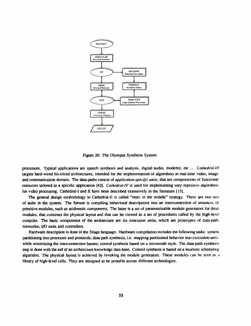
Figure 26: The Olympus Synthesis System.

processors. 1)tpical applications are speech synthesis and analysis, digital audio, modems., elc ... Cathedral-IIIlargels hard-wired bit-sliced architectures, intended for the implementation of algorithms in real-time video, imagcand communication domain. The data-paths consist of application-specific WJits, that are compositions of functionalresources tailored to a specific application [42]. Cathedral-IV is used for implementing very repelilivc algorithmsfor video processing. Cathedral-I and n have reen described extensively in the literature [15].

The general design methodology in Cathedral-II is called "meet in the middle" strategy. There are two SClsof tasks in the system. The former is compiling behavioral descriptions into an interconnection or insUlnccs or

primitive modules, such as arithmetic components. The latter is a set of parametrizable module generalOrs ror lhcsl'modules, that construct the physical layout and that can be viewed as a set of procedures called by the high-levelcompiler. The basic components of the architecture are six execution units, which are prototypes or dala-palh.

memories, 1,.0 units and controllers.Hardware description is done in the Silage language. Hardware compilation includes the following lasks: syslCm

partitioning into processes and protocols; data-path synthesis, i.e. mapping partitioned behavior into exccution-unilswhile minimizing the interconnection busses; control synthesis based on a microcode style. The data-path synthesisstep is done with the aid of an architecture knowledge data-base. ConLrol synthesis is based on a heuristic schedulingalgorithm. The physical layout is achieved by invoking the module generators. These modules call I)C s<~cn as ;\

library of high-level cells. They are designed LO re portable across different technologies.

S3

10 Conclusions.

High-level synthesis and ~timization techniques provide a means of raising the abstlaction level of the inpuldescription of a circuit and perfonning coorse-grain arca/perfonnance traoo-offs. As a result, higher pmductivily isexpected as well as higher quality cilCuits, ~use the design spiK:e can be thoroughly explored.

High-level synthesis involves computationally introctable problems. Hence heuristic algorithms are usuallyapplied, in particular to the scheduling and binding problems. Design systems have been constructed oosed onthe algorithms described here. They have been successfully used for cin;uit design in both research and produci

developmenLSeveral issues are still ~ in this field and require further investigation. First, the definitioo or a commonly

occepted language for synthesis, with precise hardware semantics as well as supP<Xt fcx interfoce description. Ind~.timing waveforms at interfoces are an integral part of design specificatioos and graphics can be more expressivethan text in this case. Second, the improvement of the algoothms for perf<Xmance-oriented design. with particularreference to synthesis and optimization of pipelined cin;uits. Last, but not least, the integration ()r high-lcvclsynthesis with logic and physical synthesis, that would pennit accurate estimation of area and delay parameters an(1their use in earlier stages of high-level optimization.

The trend towaJd larger cin;uit integration and system-level design mandates increasingly higher modclinJ,!abSb'actions and ca'reSlX>nding synthesis systems. High-level synthesis techniques will be crucial componen~ orthose CAD systems used to design competitive circuits and systems. Much fundamental and applied research i.-;n~ to solve the open problems and to insure the availability and efficiency of such systems to a large communilYof electronic designers.

11 Acknowledgements

This survey has been sponS<Xed by NSF, joinlJy wilh DEC, unoor a Presidenfjal Young Investigator Award

References

[1) A.Aoo, R.Sethi and I.Ullman, Compilers: Principles. Techniques and Tools, Addison Wcslcy. I(IRH

[2) Balakrishnan, A.Majumdar, D. Banerji, JLiitOOrs and J.Majithia, "Allocation of Mulliport Mcmorics in Oal,'Path Synthesis", IEEE Transactions on CAD, vol. CAD-7, no. 4, pp. 536-540, April 1988.

[3] T.Blackman, J.Fox and C.R~h, ""n1e Silt Silicon Compiler: Language and Features" PrIll:. ACMllEEfDesign Automation Conference, June 1985, W.232-237.

[4] F. Brewer, D. Gajski, Knowledge Based Control in Micro Architecture Design, Proceeding 24,h OA(203-209, Juoo 1987.

p.

[5] R. Cam~ano. R. A. Bergamaschi, Synthesis Using Path-based Scheduling Algorithms and Exerci.w_{. Pn)ceedings of 27'h Design Aulomalion Confereocc, Orlando, FL, June 1990, pp. 450-455.

[6] R.Cam~ano, "Pa1h-Based Scheduling for Synthesis", IEEE TransactiM on CAD, Vol CAD-If). Nn.85-93. January 1990.

PI'

54

[7] R. Camposano, W. Rosenstiel, Synthesizing Circuitsfrom Behavioral Descriptions, IEEE Trans. on CAD. Vol8, No.2, Feb 1989, pp. 171-180.

[8] R. Camposano, W. Rosenstiel, "Synthesizing Circuits from Behavioral Descriptions", IEEE 1ran.\"aclion.\" on

CAD, Vol 8, No.2, Feb 1989, p. 171-180.

(9] R. Camposano and W.Wolf, Editors, High-Level VLSI Synthesis, Kluwer Academic Publisher, 1991

[10] R. Camposano and R. Walker. Editors, A Survey of High-Level Synthesis Systems. Kluwer Academic Publi!ihcr.

1991

[11] R. CarnJX>sano, L.F. Saunders, R.M. Taret, High-Level Synthesis/rom VHDL, IEEE Design&Tcsl m Compulcrs.March, 1991

[12] G.De Micheli, P.AntogneUi and A.Sangiovanni- Vincentclli, Editors, Design Systems for VLSI C;rt:ult.'i: 1..11.1,';'Synthesis and Silicon Compilation, M.Nijhoff, 1987.

[13] G. ~ Micheli, D. Ku, F. Mailhot, T. Truong, The Olympus System for Digital Design, IEEE O<.-sign & TcSIOctober 1990, pp. 37-53.

[14] D.Gajski N.Dutt. A. Wu and S.Lin, High-Level Synthesis, Kluwer, 1992.

[15] D.Gajski, Silicon Compilation, Addison Wesley, 1988.

[16] B.PangrJe and D. Gajski, "Design Tools for Intelligent Silicon Compilation", IEEE Transactioll.'i nn CAD, vol.CAD-6, 00. 6, W. 1098-1112, November 1987.

[17] C. Gerotys and M. Elmasry. Optimal VLSI Architectural Synthesis. Kluwer Academic Publishcr~, 191)2.

[18] M. Golumbic, Algorithmic Graph Theory and Perfect Graphs, Academic Press, 1980.

[19] G.Goossens, J. Vandewalle and H.De Man, "Loop Optimization in Register-Transfer level schc<hlling ror DSPsystems", Proceedings of the ACMIIEEE Design Automation Conference, 1989, pp. 826-831.

[20] L. Hafer, A. Parker, "Automated Synthesis of Digital Hardware", IEEE Transaction on Computer.{, Vol (,-~1No 2, February 1982.

[21] T.C.Hu, "parallel Sequencing and Assembly Line Problems", Operations Research, No.9. pp. R41-R4R.

[22] K.Hwang, A.Casavant, M.Dragomirecky and M. d' Abreu, "Constrained Conditional Resource Sharing inPipeline Synthesis", lCCAD, Proceedings of the International Conference on Computer-Aided De.~if!,n. pp.52-55, 1988.

[23] J.Huisken. HJanssen. PLippens. O.McArdle. R.Segers. P.Zegers, A. Delaruelle and J. van Mccrbergen, E.{!i

cient Design of Systems on Silicon with PYRAMID, in Logic and Architecture Synthesi.\" for .\"ilic(ln Compiler.\.

North Holland. Amsterdam. 1989.

[24] C.-T.Hwang, J.-H. .Lee and Y-C Hsu, "A Formal Approoch to the Scheduling Problem in High-l.evel Synthcsis", IEEE Transaction on CAD, Vol CAD-1O, No.4, pp. 464-475, April 1991.

55

[25] O.Karatsu, "VLSI Design Standardization Effort in Japan, Proceedings of the Design AUlomatinn Co'!ferenc('

1989, pp.So-SS.

[26] D.Knapp "Synthesis from Partial Sb"UCture", in D. Edwards, Editor, Design Methodologies {nr VIAS! and

Computer Architecture, pp. 35-51, Elsevier Science Publications, 1989.

[27] D. W. Knapp, Manual Rescheduling and Incremental Repair of Register-Level Datapaths. Pn)C,~ ICCAD-R9

Santa Clara, CA. Nav 1989. pp 58-61.

[28] D. W. Knapp Feedlxlck Driven Datapath Optimization in Fasolt ICCAD-90. Santa Clara. California. Novcmrer

1990. pp.300-303

[29] T. Kowalski, An Artijiciallntelligence Approach to VLSI Design, Boston, MA; Kluwer Academic Publishers.

1985.

[30] D.Ku, G.De Micheli, High-Level Synthesis of ASICS under Timing and Synchronization Con.\"trainl.\". KI\I~'cr

1992.

[31] D. Ku, G. De Micheli, Relative Scheduling Under Timing Constraints, Proceedings 0/27 th De.\"iJ!,n Autom(ll;nn

Conference, Orlando, Florida, June, 1990.

[32] D.Ku and G. De Micheli, .. Relative Scheduling under Timing Constraints: Algorithms for High-Level Syn

thesis of Digital Circuits"1EEE Transactions on CADI/CAS. Vol. 11, No.6, April 1992, pp. 6%-718.

[33] D. Ku, G. De Micheli, "Constrained Resource Sharing and Conflict Resolution in Hebe", fnlf~gralinn.VLSI Journal, Vol. 12, No.2, December 1991, pp. 131-166.

[34] D. Kuck, The Structure of Computers and Computation, Wiley, 1978.

[35] C. Leiserson, F. Rose, and J. Saxe. "Optimizing Synchronous Circuitry by Retiming." Proceedi,,}!,,\' C!f the .~rdCalrech Conference on Very Large Scale Integration, 1983.

[36] Y.Liao and C. Wong, "An Algorithm to Com~ct a VLSI Symbolic Layout with Mixed Con~'rainl~". IFEI;

Transactions on CADI/CAS, Vol CAD-2, No.2. April 1983. pp.62-69.

[37] RLipsett. C. Schaefer and C.Ussery. VHDL: Hardware Description and Design, Kluwer, 1~1

[38) M. McFar]and, A.Parker and R. Camposano, The High-level Synthesis of Digital Systems, Proc('e,dings or Ihl'IEEE, Vol. 78, No.2, February 1990, pp. 30]-3]8.

[39] M. J. McFarland, "Reevaluating the Design Space for register Transfer Hardware SynLhcsi!i.'. ICCAD. Prn.ceedings of the International Conference on Computer-Aided Design, pp. 184-187, 1987.

[40] M. J. McFarland, "Using Bottom-Up Design Techniques in the Synthesis of Digital Hardware frmn Ahslr(j('Behavioral Descriptions", Proceedings 23th Design Automation Conference, June 1986, p. 474-4R().

[41] P.Michel, U.Lau~r and P.Duzy, The Synthesis Approach to Digital System Design. Kluwcr. I9c:J2.

[42] S.Note, W.Geurts, F.Chauor and H.DeMan, "Cathedral-III: Architecture-driven High-lcvcl Synthesis r(}r High

throughput DSP applications", Proc. Des AU/om. Coni, 1991, pp. 597-602.

~

[43] A. Parker, J. Pizarro, M. Mlinar, MAHA: A Program for Data Path Synthesis, Proceedings 23th Design

Automation Conference, June 1986, p. 461-466.

[44] N.Park and A.Parker "Sehwa: A Software P~kage for Synthesis of Pipelines from Behavioral S~ificalions'

IEEE Transaction on CAD, Vol CAD-7, No.3, pp. 356-370, March 1988.

[45] P.Paulin and J.Knight. "Force-~ted Scheduling for the Behavioral Synthesis of ASIC's". /EEF. Tran.\"(ICI;(ln

on CADI/CAS. Vol CAD-8. No.6. pp. 661-679. July 1989.

[46] P. G. Paulin, J. P. Knight, E. F. Girczyc, HAL: A Multi-Paradigm Approach to Automatic Data-ptlth Synthe.~i.~

Proceedings 23th Design Automation Conference. June 1986. pp. 263-270.

[47] B.Preas and MLorenzetti. Physical Design Automation of VLSI Systems, Benjamin Cummings Wesley, 198R.

[48] J.Southard, "MacPius, An Approach to Silicon Compilation", fEEE Computer, Vol 16, No. 12, [)(x:cmber

1983, pp. 59-70.

[49] D. Springer and D. Thomas, "Exploiting the Special Structure Of Conflict and Compatibility Graphs in High.

Level Synthesis", ICCAD, Proceedings of the International Conference on Computer-Aided Dc.\"i.l,'n, pp.254

259, 1990.

[50] L. Stok, Architecture Synthesis and Optimization of Digital Systems, Ph.D. Dissertation, Eindhovcn Univ~ily

The Netherlands, 1991.

[51) D. Thomas, E.Lagnese, R. Walker, J.Nestor, J.Rajan and R.Blackbum, Algorithmic and Regi.\"tcr 1'rcln.ifcr Levc'

Synthesis: The System Architect's Workbench, Kluwer Academic Publisher, 1990

[52] D. Thom~, C. Hitchcock III, T. Kowalski, J. Rajan, R. Walker, Automatic Data Path Synthesi.~. IEEE Crunputcr

magazine, December 1983.

[53] D.Thomas and P. Moorby, The Verilog Hardware Description Language, Kluwer, 1991

[54] H.Trickey, "FIamel: A High-Level Hardware Compiler", /EEE Transaction on CADI/CAS, vol. CAO-6. No.

2, pp.259-269, March 1987.

[55] C. Tseng, D. Siewiorek, "Automated Synthesis of Data Paths in Digital Systems", I EEE Tran.~(It::li(/n (/n CAD,

Vol CAD-5, pp. 379-395, July 1986.

Proc !fith[56] G.Zimmermann, "The MIMOLA Design System: Detailed Description of the Soflware Sysl(~m

Des Autom. Con/. 1979, pp 56-63.

57