A Technical Report by

Kyle AndersonChad Burdyshaw

and

Steve Karman

UTC-CECS-SimCenter-2008-02May 2008

Geometry ParameterizationUsing Control Grids

7 0 1 E a s t M . L . K i n g B o u l e v a r d • C h a t t a n o o g a , T N 3 7 4 0 3

G R A D U A T E S C H O O L O F C O M P U T A T I O N A L E N G I N E E R I N G

Table of Contents

Acknowledgements............................................................................................. ii

Abstract............................................................................................................... iii

Introduction.......................................................................................................... 1

Control Grids for Parameterization...................................................................... 2

Results................................................................................................................. 9

Summary............................................................................................................ 14

References..........................................................................................................15

i

Acknowledgements

In 1984, the State of Tennessee created a Center of Excellence program for public institutions of higher education within the state. The purpose of these centers, known as THEC (Tennessee Higher Education Commission) Centers of Excellence, is to build on the strength of the Stateʼs universities, expand the Stateʼs research base, and increase its national and international stature and economic competitiveness. The research reported herein was carried out under the auspices of the THEC Center of Excellence for Applied Computational Science and Engineering under the direction of Dr. Harry McDonald at the University of Tennessee at Chattanooga under the project entitled “Adjoint-Based System for Design Optimization.” This support is gratefully acknowledged.

ii

Abstract

A technique is described for parameterizing geometries in a manner suitable for numerical simulations used in design optimization. The methodology is flexible, easy to use, extendable, and is applicable for multidisciplinary design optimization. The parameterization technology is described and demonstrated in both two and three dimensions.

iii

1. Introduction

The use of numerical simulations for analyzing existing geometries is now routinely used in many industries. The simulations are also often used to conduct trade-off studies for evaluating options that may lead to improved performance. In recent years, numerous researchers have been developing formal methods of determining sensitivity derivatives that can be used in conjunction with numerical optimization techniques to systematically reduce one or more cost functions that will subsequently lead to better performance of the vehicle in question (see for example [ 3-6, 9-10, 12-14, 18-19]). For applications where the shape is allowed to change to achieve the desired performance, it is necessary to describe either the geometry, or changes to the geometry, in terms of a set of parameters that are used as design variables to drive the optimization procedure. Example methodologies that have been utilized include the use of the individual mesh points on the surface of the mesh [13-14], Bezier, B-spline, and NURBS surfaces [4, 11, 20-21], Hicks-Henne functions[12], sine functions [10], discipline specific functions [24], and free-form deformation [22-23]. A summary of some of the more prevalent parameterization techniques is given in Ref. [21]. Of particular interest is the method of free-form deformation (FFD) because it provides a convenient method for multidisciplinary design optimization (MDO) applications where it may be necessary to modify several unrelated meshes simultaneously. The FFD method uses a three-dimensional mesh where each node in the mesh is considered to be a control point of a NURBS volume. The position of the nodes are used as the design variables so that as the control points are repositioned during the design process, the NURBS volume is re-evaluated to provide changes to the original geometry. Although effective, in the most general implementation, the number of design variables can be large if the mesh of control points is fully three dimensional. This is due to the fact that the number of nodes in the mesh increases as the cube of the number of points placed along one side of the mesh. In reference [23] a methodology is described that alleviates the cubic dependence on the number of design variables to a quadratic dependence by replacing a trivariate FFD volume with a bivariate FFD surface that is placed onto the surface of the geometry.

In the present work, a technique for parameterizing geometries is described that has many of the advantageous features of FFD while also reducing the growth of design variables to be quadratic as the number of design variables along a one-dimensional direction is increased. Furthermore, the present technique utilizes a grid that is fixed throughout the design process. This is in contrast to the FFD technique in which the control points are continuously moved and can potentially become tangled.

1

In developing the present technique, the following requirements are considered:1. Fast and easy to use2. Applicable for MDO3. Extendable to new situations as they arise4. Produce smooth geometries5. Allow for large deformations6. Does not require a significant number of design variables7. May be applied to large or small regions of the geometry to be designed8. Provides reasonably easy application of constraints9. Accurate sensitivity derivatives are readily obtained

The methodology described here provides a viable alternative to the FFD technique and satisfies the above set of requirements.

2. Control Grids for Parameterization

Although control grids may be used for both two- and three-dimensional applications, their use for parameterization is most easily described by initially considering a two-dimensional example. Figure 1 depicts an airfoil that is to be parameterized, along with an exemplary control grid surrounding the airfoil. To easily identify the geometry in the figure, the airfoil is depicted as a line, although in the present context it is actuality comprised of a series of mesh points defining the surface. These mesh points are typically part of a larger volume mesh. To use the control grid to modify the shape of the geometry, a set of partial differential equations with appropriate boundary conditions is discretized and solved on the control grid. The solutions of the discrete set of equations are considered as perturbations to the original surface and are interpolated and added to the points defining the original geometry. For use in shape optimization algorithms, the design variables stem from the boundary conditions associated with the partial differential equation.

Figure 1. Control grid surrounding an airfoil

2

As a specific example, it is noted that a requirement specified earlier is that perturbations to the geometry be generally smooth. In this way, an initially smooth geometry will remain smooth after perturbations are added. This leads one to consider the use of elliptic partial differential equations such as Laplace-type equations for each direction or equations for linear elasticity. However, it should be noted that the use of a partial differential equation is not required. In the present work, a simple approximation to a Laplacian is used to smoothly propagate perturbations in each direction independently. For the present results, the approximation to the Laplacian in the interior of the mesh is based on inverse distance weighting, although simple averaging has also been used. Dirichlet boundary conditions are typically used at external boundaries of the control grid, although internal boundaries may also be considered as described in a later section. Separate boundary conditions are applied to individual points on the boundaries of the control grid, and it is the magnitude of the boundary conditions that become the design variables used to modify the shape. The boundary conditions for perturbations in each direction are determined by specifying them to be either normal to the control grid, tangent to the control grid, normal to the surface of the geometry, or in an otherwise pre-specified direction. The individual Cartesian components or the directions of the perturbations could also be used as design variables, although using the magnitude of the perturbation reduces the number of design variables and allows for better control. For example, if one wishes to control the thickness of a geometry that is not aligned with a coordinate axis, the control grid would be aligned with the geometry and perturbations normal to the upper and lower boundaries of the control grid could be obtained.

With the smoothing procedure described above, the number of design variables is proportional to the number of mesh points lying on the boundaries of the control grid. This represents a reduction in the number of design variables in comparison with a free-form deformation technique, which requires the number of design variables to be proportional to the total number of points in the entire grid.[23] A further reduction in the number of design variables is obtained by defining a “design grid”, which is coarser than the control grid but has the same general shape. The design variables are associated with points lying on the boundaries of the design grid and the boundary conditions for the control grid are obtained by interpolation. An example is given in Fig. 2 for a two-dimensional control grid. Here, the design grid consists of a series of points defined on each boundary of the control grid. Note that the number of points on each boundary are not required to be the same, as the otherwise double valued points at the corners of the control grid are not used in the smoothing procedure because the computational stencil only utilizes points immediately connected the central point. Furthermore, in some applications it may be advantageous to define boundary conditions that are applied to larger regions of the control grid. A natural example would be specifying a single boundary condition that is applied around the entire perimeter of an axisymmetric control grid.

3

Figure 2. Control grid including depiction of points on design grid surface

An example of using a control grid to manipulate a geometry is shown in Fig. 3. In this example, the initial geometry corresponds to an NACA 0012 airfoil, which is placed approximately in the center of the control grid. The smoothing procedure is applied in each direction independently and the boundary conditions are specified so that perturbations are only allowed in the vertical direction. As seen in the figure, the new airfoil geometry is greatly modified from the original and the contours of the perturbations are smooth. Note also from the figure that the modified geometry extends beyond the boundaries of the control grid. Because the perturbations are relative to the original geometry and because the control grid is fixed, large deformations can be obtained with no tangling of the control grid which could happen with free-form deformation.

Figure 3 Example deformation using control grid

During the design process, mesh sensitivities are generally required as the geometry deformations at the surface are propagated into the interior. The means for propagating the interior mesh points is not generally dependent on the parameterization of the surface and can be accomplished with many techniques [see e.g. 3, 18]. However, the determination of mesh sensitivities inevitably requires the sensitivity derivatives of the surface mesh points with respect to the design variables. Because of the linearity of the present smoothing algorithm and because the geometry is always perturbed in relation to the original shape, the sensitivities of the surface points with respect to the design variables are easily obtained by sequentially setting each design variable to unity while setting the remainder of the boundary conditions to zero. After solving the equations, the solution corresponds to the sensitivity derivatives. While this parameterization technique requires the solution of the perturbations for each design variable, the sensitivity derivatives of the surface points are fixed throughout the design process so the solution

4

of the perturbations is only required at the initial step and need not be repeated during each design cycle. Again, this is because of the linearity of the smoothing procedure and because the geometry is always modified in relation to the original geometry. In addition, efficient procedures, such as multigrid acceleration, may be used to obtain rapid convergence. Finally, it should be noted that control grids may be relatively coarse and that a highly converged solution is not generally required, provided that the boundary conditions propagate into the interior.

To examine the ability of the current procedure to obtain general shapes while not producing high-frequency oscillations, an NACA 0012 airfoil is used as an initial geometry and a target geometry is obtained by randomly moving points on the lower surface of the airfoil. A single control grid is used where vertical perturbations are allowed on the top and bottom boundaries and zero perturbations are prescribed on the left and right sides of the control grid. The control grid has 201 points in the horizontal direction and 81 points in the vertical direction. There are 32 design variables evenly spaced on the upper and lower boundaries for a total of 64 design variables. Fig. 4a depicts the original airfoil geometry, the current geometry, and the target geometry. The current geometry is obtained after 10 design cycles using a trust-region method [15] and the cost function is the squared difference between the coordinates of the current geometry and the target geometry. Fig. 4b shows contours of the perturbations in the control grid as well as the final geometry. As seen in Fig. 4a, the present method reproduces the target geometry reasonably well although it does not capture the higher-frequency oscillations near the leading edge. Increasing the number of design variables may capture this high-frequency oscillation. Note that from the contours depicted in Fig. 4b, the design variables successfully adjust to produce the oscillations on the lower surface while reasonably maintaining the original geometry on the upper surface. It should be noted that repeating this experiment using several control grids of varying extent in the vertical direction from 0.1 to 0.5 has very little effect on the final answer.

5

0 0.2 0.4 0.6 0.8 1

x

-0.15

-0.1

-0.05

0

0.05

0.1

0.15y

NACA 0012

Current

Target

Figure 4a. Original, current, and target geometries

Figure 4b. Boundaries of control grid and contours of y-perturbations

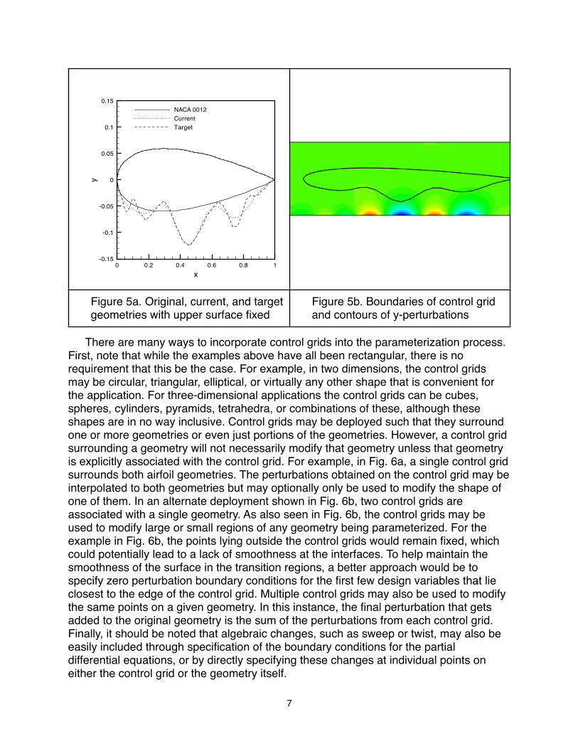
In the results shown in Fig. 4, the upper surface points have been approximately held fixed by explicitly including them in the cost function. With close examination, however, a very slight variation between the current geometry and the original geometry can be seen on the upper surface approximately ten percent aft of the leading edge. A more direct way to hold the upper surface fixed is to simply place the control grid so it only effects the geometry points on the lower surface of the airfoil. Although using this technique may be suitable in some instances, a more general procedure is to initially determine the points in the control grid that surround the constrained geometry points, and then simply specify zero perturbations at those points during the solution procedure. This method is easily automated and can be viewed as enforcing internal boundary conditions during the solution for the perturbations.

Figure 5 depicts results obtained using the internal boundary condition procedure for the same problem shown earlier in Fig. 4. As seen in Fig. 5a, the fidelity of the upper surface is successfully maintained while the lower surface is allowed to change. Further, from the contours of the perturbations shown in Fig. 5b, the perturbations appear to be smooth. However, it should be noted that the geometry at the interface between the fixed points and the points that are allowed to move may not be smooth, particularly if the perturbations at the adjoining points are large. This is because the fixed point is essentially a boundary between the fixed curve and the variables curve.

6

0 0.2 0.4 0.6 0.8 1

x

-0.15

-0.1

-0.05

0

0.05

0.1

0.15y

NACA 0012

Current

Target

Figure 5a. Original, current, and target geometries with upper surface fixed

Figure 5b. Boundaries of control grid and contours of y-perturbations

There are many ways to incorporate control grids into the parameterization process. First, note that while the examples above have all been rectangular, there is no requirement that this be the case. For example, in two dimensions, the control grids may be circular, triangular, elliptical, or virtually any other shape that is convenient for the application. For three-dimensional applications the control grids can be cubes, spheres, cylinders, pyramids, tetrahedra, or combinations of these, although these shapes are in no way inclusive. Control grids may be deployed such that they surround one or more geometries or even just portions of the geometries. However, a control grid surrounding a geometry will not necessarily modify that geometry unless that geometry is explicitly associated with the control grid. For example, in Fig. 6a, a single control grid surrounds both airfoil geometries. The perturbations obtained on the control grid may be interpolated to both geometries but may optionally only be used to modify the shape of one of them. In an alternate deployment shown in Fig. 6b, two control grids are associated with a single geometry. As also seen in Fig. 6b, the control grids may be used to modify large or small regions of any geometry being parameterized. For the example in Fig. 6b, the points lying outside the control grids would remain fixed, which could potentially lead to a lack of smoothness at the interfaces. To help maintain the smoothness of the surface in the transition regions, a better approach would be to specify zero perturbation boundary conditions for the first few design variables that lie closest to the edge of the control grid. Multiple control grids may also be used to modify the same points on a given geometry. In this instance, the final perturbation that gets added to the original geometry is the sum of the perturbations from each control grid. Finally, it should be noted that algebraic changes, such as sweep or twist, may also be easily included through specification of the boundary conditions for the partial differential equations, or by directly specifying these changes at individual points on either the control grid or the geometry itself.

7

Figure 6a. Single control grid surrounding two geometries

Figure 6b. Multiple control grids associated with a single geometry

Note that for internal flows, a situation can occur using the present technique which will be referred to as “blocking.” Referring again to Fig. 6a, if the design variables are placed only at the external boundaries of the control grid and the upper surface of the top airfoil and the lower surface of the bottom airfoil are held fixed using the procedure described in reference to Fig. 5, the perturbations prescribed on the external boundaries could be prevented from propagating into the interior of the control grid. In many applications this is easily remedied by simply using a separate control grid for each geometry. In three-dimensional applications, it may be also be desirable to modify the internal surface of a geometry while holding the outer surface fixed. A typical example would include the design of the internal shape of an inlet while holding the outer mold lines of the nacelle fixed. Blocking may be alleviated using several techniques. The easiest method is to simply ensure that the control grid is finer than the defining points on the geometry so that the perturbations are allowed to propagate between the fixed points and into the interior of the control grid. Although not shown, this approach has been successfully used. Alternatively, a control grid may be placed between the two surfaces so that only the interior surface will be modified. Other approaches would include simply using some of the points in the interior of the control grid as design variables, incorporating source terms into the partial differential equations, using Neumann boundary conditions, or by devising a suitable control grid with a passage through it (for example, a hollow tube). In the latter case, design variables would be placed on the inner and outer surfaces of tube.

8

3. Results

Results are given below for both two and three-dimensional applications. In the two dimensional applications, an unstructured Euler solver similar to that described in Ref. [1] is used to determine the variables in the flow field, while sensitivity derivatives are obtained using the complex-variable method of forward-mode differentiation described in Refs. [2, 16-17]. Although the examples are for inviscid flows, it should be noted that the parameterization method is only used to modify surface points and is thus applicable to viscous flows as well.

In the first example, the initial geometry is an NACA 0012 airfoil at a free-stream Mach number of 0.5 and an angle of attack of 1.25 degrees. The goal of the design is to increase the lift coefficient from its initial value of 0.17 to a target value of 1.0. For this test, two control grids are used and the design is repeated separately for each. In each case, the design variables on the upper and lower surfaces of the control grid provide perturbations in the vertical direction, while the design variables on the left and right sides of the control grid are held constant at zero. In the first control grid, shown in Fig. 7a, the leading edge of the airfoil is placed a specified distance from the left side of the control grid, while the trailing edge is placed adjacent to the right side of the control grid. Because the perturbations on the right-hand-side of the control grid are zero, the effect of this placement is to allow the vertical position of the leading edge to change while the trailing edge is held fixed. Note that the trailing edge could also be held fixed using the approach described earlier. The second control grid, depicted in Fig. 7b is constructed so that the leading and trailing edges of the airfoil are both placed adjacent to the boundaries of the control grid, thereby effectively fixing those points.

Figure 7a. Control grid boundaries and y-perturbations: Leading edge floating, trailing edge fixed

Figure 7b. Control grid boundaries and y-perturbations: Leading and trailing edges fixed

After only 2 design cycles using a trust-region method [15], the final lift coefficient is successfully obtained for each case. As seen in Fig. 8a, the resulting pressure distributions show significant changes in comparison to that for the baseline NACA 0012. In addition, the pressure distributions for the modified geometries are each somewhat different, reflecting the effectively different constraints on the geometries. As

9

seen in Fig. 8b, the modified geometries are similar although they are significantly different from the original. Furthermore, Fig. 8c shows a close-up of the leading edge geometries and illustrates the differences obtained using the different parameterizations. In particular, when using the first control grid, the leading edge of the airfoil is slightly raised when compared to the other geometries.

0 0.2 0.4 0.6 0.8 1

x

-2

-1.5

-1

-0.5

0

0.5

1

Cp

NACA 0012

Modified (LE floating, TE fixed)

Modified (LE fixed, TE fixed)

0 0.2 0.4 0.6 0.8 1

x

-0.4

-0.2

0

0.2

0.4

y

NACA 0012

Modified (LE floating, TE fixed)

Modified (LE fixed, TE fixed)

0 0.05 0.1 0.15 0.2 0.25 0.3

x

-0.1

-0.05

0

0.05

0.1

0.15

0.2

y

NACA 0012

Modified (LE floating, TE fixed)

Modified (LE fixed, TE fixed)

Figure 8a. Pressure distributions

Figure 8b. Original and modified geometries

Figure 8c. Original and modified geometries near leading edge

A final two-dimensional example is shown in Figs. 9 and 10 for a transonic slotted airfoil originally described in Ref. [27]. For the case considered here, the Mach number and angle of attack are 0.7 and 1.0 degrees, respectively. The cost function is defined as a linear combination of the lift and drag coefficients so that the lift will remain approximately constant while simultaneously reducing the drag. The lift on the baseline configuration is 0.1359 with a corresponding drag coefficient of 0.0402. Figure 9a depicts the initial and final shapes of the main element and the flap, whereas Fig. 9b shows the control grid as well as the contours of vertical perturbations after the design. For this case, the control grid is not rectangular and contains 101 points in the direction approximately aligned with the free stream and 41 points in the normal direction. Only 7 design variables are used on the top and bottom boundaries of the control grid, for a total of 14 design variables. As seen in Fig. 9b, the control grid extends ahead of and behind the airfoil. The trailing edge of each airfoil is held fixed by specifying internal boundary conditions as described earlier.

After ten design cycles, the final lift and drag coefficients are 0.1351 and 0.0222 respectively, resulting in a 40% decrease in drag coefficient. It is seen in Fig. 9a that the upper and lower surfaces of the modified airfoil near the leading edge of the main element are slightly lower than the baseline geometry, although the overall thickness is approximately unchanged. Toward the aft end of the main element, the upper surface is slightly above the original surface whereas the lower surface is only very slightly raised. Consequently, the thickness at the aft end of the main element is increased. The geometry of the flap on the modified airfoil appears to be only slightly changed over that

10

of the original geometry. Density contours for the baseline and modified geometries are shown in Figs. 10a and 10b. After the design, the shock on the main element is not eliminated but is smaller in extent when compared to the baseline configuration.

0 20 40 60 80 100

x

-40

-20

0

20

40

y

Baseline Main

Baseline Flap

Modified Main

Modified Flap

Figure 9a. Original and modified geometry for slotted airfoil

Figure 9b. Control grid boundaries and vertical perturbations for slotted airfoil

Figure 10a. Density contours for baseline slotted airfoil

Figure 10b. Density contours for modified slotted airfoil

11

The control-grid methodology has also been developed and tested for three-dimensional applications. For these applications, the flow solver developed at the University of Tennessee at Chattanooga [25,26] is used for analysis of the flow field, gradients are obtained using the adjoint solver as described in Refs. [7-8], and the PORT trust-region optimization code is used [15].

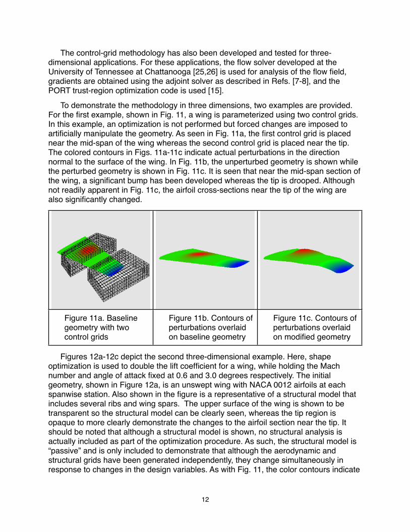
To demonstrate the methodology in three dimensions, two examples are provided. For the first example, shown in Fig. 11, a wing is parameterized using two control grids. In this example, an optimization is not performed but forced changes are imposed to artificially manipulate the geometry. As seen in Fig. 11a, the first control grid is placed near the mid-span of the wing whereas the second control grid is placed near the tip. The colored contours in Figs. 11a-11c indicate actual perturbations in the direction normal to the surface of the wing. In Fig. 11b, the unperturbed geometry is shown while the perturbed geometry is shown in Fig. 11c. It is seen that near the mid-span section of the wing, a significant bump has been developed whereas the tip is drooped. Although not readily apparent in Fig. 11c, the airfoil cross-sections near the tip of the wing are also significantly changed.

Figure 11a. Baseline geometry with two control grids

Figure 11b. Contours of perturbations overlaid on baseline geometry

Figure 11c. Contours of perturbations overlaid on modified geometry

Figures 12a-12c depict the second three-dimensional example. Here, shape optimization is used to double the lift coefficient for a wing, while holding the Mach number and angle of attack fixed at 0.6 and 3.0 degrees respectively. The initial geometry, shown in Figure 12a, is an unswept wing with NACA 0012 airfoils at each spanwise station. Also shown in the figure is a representative of a structural model that includes several ribs and wing spars. The upper surface of the wing is shown to be transparent so the structural model can be clearly seen, whereas the tip region is opaque to more clearly demonstrate the changes to the airfoil section near the tip. It should be noted that although a structural model is shown, no structural analysis is actually included as part of the optimization procedure. As such, the structural model is “passive” and is only included to demonstrate that although the aerodynamic and structural grids have been generated independently, they change simultaneously in response to changes in the design variables. As with Fig. 11, the color contours indicate

12

the size of the perturbations that are applied to the original geometry after the optimization.

The control grid, shown in Fig. 12b, has only 11 points in the spanwise direction with a 21x11 grid in the plane normal to the span. Although not shown, a 6x6x2 design grid is used, with only 2 planes of design variables in the spanwise direction. To transfer the design variables from the design grid to the control grid, linear interpolation is first used along each of the twelve edges to determine boundary conditions for the control grid along these edges. Note that boundary conditions on each of the six faces of the control grid are typically determined using linear interpolation from the design grid. However, in this application, in the plane of the control grid nearest the wing tip, a smoothing procedure similar to that used for two-dimensional applications is first used instead of linearly interpolating the data from the design grid. The data on the remaining planes is then determined using linear interpolation from the points on the design grid to those on the control grid. The entire volume is then smoothed to propagate the perturbations at the boundaries into the interior. In this application, the only non-zero design variables are those that lie on the upper and lower line segments defining the plane nearest the wing tip. Combined with the fact that only two spanwise planes are used for the design grid, the effect is that modifications are made to the geometry of the airfoil sections near the tip, which decrease linearly as the wing root is approached. In this manner, changes in the airfoil profiles may be introduced without the possibility of simultaneously causing spanwise oscillations so the airfoil sections vary smoothly between the wing tip and the root. This procedure is referred to as “face smoothing.” As seen in Fig. 12b, after the optimization is complete, larger perturbations are evident on the face of the control grid nearest the tip, which subsequently decrease as the root is approached.

After only two design cycles, the target lift has been achieved to eleven decimal places. As shown in Fig. 12c, the final geometry exhibits noticeably more camber at the tip, which decreases linearly to zero at the wing root. As also observed, the structural model has also been deformed in response to changes in the design variables, and remains congruent with the aerodynamic model.

13

Figure 12a. Baseline aerodynamic and structural models

Figure 12b. Control grid with contours of perturbations

Figure 12c. Final aerodynamic and structural models

4. Summary

A new procedure has been developed to parameterize geometries for use in design optimization. The technique shares many of the positive qualities of parameterizations based on free-form deformation including the fact that it may be used in multidisciplinary applications. However, the number of design variables can be reduced when compared to free-form deformation so they increase as the square of the size of the design grid instead of cubicly. Further, the control grid is held fixed during the entire design cycle, preventing it from folding on itself and thereby allowing very large deformations. The method has been implemented in both two and three dimensions and exemplary designs have been demonstrated.

14

5. References

1. Anderson, W. K., and Bonhaus, D. L., “An Implicit Upwind Algorithm for Computing Turbulent Flows on Unstructured Grids,” Computers and Fluids, Vol. 23, No. 1, (1994), pp. 1-21.

2. Anderson, W. K., Newman, J. C., and Whitfield, D. L., and Nielsen, E. J., “Sensitivity Analysis for the Navier-Stokes Equations on Unstructured Meshes Using Complex Variables,” AIAA J., Vol. 39, No. 1, (2001), pp. 56-63.

3. Anderson, W. K., and Venkatakrishnan, V., “Aerodynamic Design Optimization on Unstructured Grids with a Continuous Adjoint Formulation,” Computers and Fluids, Vol. 28, No. 4-5, (1999), pp. 443-480.

4. Anderson, W. K., and Bonhaus, D. L., “Airfoil Design on Unstructured Grids for Turbulent Flows,” AIAA J., Vol. 37, No. 2, (1999), pp. 185-191.

5. Angrand, F., “Optimum Design for Potential Flows,” Int. J. Num. Methods in Fluids, Vol. 3, (1983), pp. 265-282.

6. Burdyshaw, C. E., “Quasi 3D Multi-Stage Turbomachinery Pre-Optimizer,” M.S. Thesis, Mississippi State University, 2001.

7. Burdyshaw, C. E., and Anderson, W. K., “A General and Extendible Unstructured Mesh Adjoint Method,” J. of Aerospace Computing, Information, and Communication, Vol. 2, No. 10, (2005)

8. Burdyshaw, C. E., “Achieving Automatic Concurrency Between Computational Field Solvers and Adjoint Sensitivity codes,” Ph.D. Thesis, University of Tennessee, Chattanooga, May, 2006.

9. Burgreen, G. W., and Baysal, O., “Three-Dimensional Aerodynamic Shape Optimization of Wings Using Sensitivity Analysis,” AIAA Paper 94-0094, Jan. 1994.

10.Drela, M., “Design and Optimization Method for Multi-element Airfoils,” AIAA Paper 93-0969, Feb. 1993.

11.Fudge, D. M., and Zingg, D. W., “A CAD-Free and a CAD-Based Geometry Control System for Aerodynamic Shape Optimization,” AIAA Paper 2005-0451.

12.Hicks, R. M., and Henne, P. A., “Wing Design by Numerical Optimization,” J. of Aircraft, Vol. 15, No. 7, (1978), pp. 407-412.

13.Jameson, A., “Aerodynamic Design Via Control Theory,” J. Scientific Computing, Vol. 3, (1988), pp. 233-260.

14.Jameson, A., Alonso, J. J., Reuther, J., Martinelli, L., and Vassberg, J. C., “Aerodynamic Shape Optimization Techniques Based On Control Theory,” AIAA Paper 98-2538.

15

15.Kaufman, L., and Gay, D., “PORT Library: Optimization and Mathematical Programming. Bell Laboratories, May, 1997.

16.Newman, J. C., Anderson, W. K., and Whitfield, D. L., “Multidisciplinary Sensitivity Derivatives Using Complex Variables,” MSSU-COE-ERC-98-08 (Mississippi State University)

17.Newman, J. C., Anderson, W. K., and Whitfield, D. L., “A Step-Size Independent Approach to Multidisciplinary Sensitivity Analysis,” J. of Aircraft, Vol. 40, No. 3, (2003) pp. 566-573

18.Nielsen, E. J., and Anderson, W. K., “Recent Improvements in Aerodynamic Optimization on Unstructured Meshes,” AIAA J., Vol. 40, No. 6, (2002), pp. 1155-1163.

19.Nielsen, E. J., and Anderson, W. K., “Aerodynamic Design Optimization on Unstructured Meshes Using the Navier-Stokes Equations,” AIAA J., Vol. 37, No. 11, (1999), pp. 1411-1419.

20.Samareh, J. A., “A Novel Shape Parameterization Approach,” NASA TM/TM-1999-209116, May, 1999.

21.Samareh, J., A., “A Survey of Shape Parameterization Techniques for High-Fidelity Multidisciplinary Shape Optimization,” AIAA J., May, 2001, pp. 877-884.

22.Samareh, J. A., “Multidisciplinary Aerodynamic-Structural Shape Optimization Using Deformation (MASSOUD),” AIAA Paper 2000-4911.

23.Samareh, J. A., “Aerodynamic Shape Optimization Based on Free-Form Deformation,” AIAA Paper 2004-4630

24.Smith, R. E., Bloor, M. L. G., Wilson, M. J., and Thomas, A. M., “Rapid Airplane Parametric Input Design,” AIAA Paper 95-1687.

25.Sreenivas, K., Hyams, D. G., Nichols, D. S., Mitchell, B., Taylor, L. K., Briley, W. R., and Whitfield, D. L., “Development of an Unstructured Parallel Flow Solver Ffor Arbitrary Mach Numbers,” AIAA Paper No. 2005-0325, Jan. 2005.

26.Sreenivas, K., Taylor, L., and Briley, R., “A Global Preconditioner for Viscous Flow Simulations at All Mach Numbers,” AIAA-2006-3852, June 2006.

27.Whitcomb, R. T., and Clark, L. R., “An Airfoil Shape for Efficient Flight At Supercritical Mach Numbers,” NASA TM X-1109, 1965.

16