geometric comparison of popular mixture model...
TRANSCRIPT

Journal of Modern Mathematics Frontier Vol. 1 Iss. 4, December 2012
Geometric Comparison of PopularMixture Model DistancesScott A. Mitchell
Computing Research, Sandia National Laboratories, U.S.A.
Abstract
Triangular discrimination, Jensen-Shannon divergence, andthe square of the Hellinger distance, are popular distancefunctions for mixture models, and are known to be similar.Here we expound upon their equivalence in terms of theirfunctional forms after transformations, factorizations, and se-ries expansions, and in terms of the geometry of their con-tours. The ratio between these distances is nearly flat for mod-est ratios of point coordinates, up to about 4:1. Beyond thatthe functions increase at different rates. We include deriva-tions of ratio bounds, and some new difference bounds. Weprovide some constructions that nearly achieve the worst-cases. These help us understand when the different func-tions would give different orderings to the distances betweenpoints.
Keywords
Mixture Models; Geometry; Distance Functions
Introduction
Mixture models are ubiquitous in statistics and theirapplications. Mixture models express quantities whosecomponents are positive and sum to one. They con-veniently express a discrete probability distribution forexclusion settings, where probabilities sum to one; seeDeza and Deza [6] for a formal definition. They also ex-press fractions of a whole, e.g. they frequently arise af-ter normalization. They are geometrically equivalent topoints lying on a regular simplex. See Appendix “DataModel and Application Context” for how a mixturemodel arises in one information application.
A distance function measures how close two pointsare to one another. In clustering applications, pointsthat are close to each other based on this distance aregrouped together. Nearest-neighbors often play a spe-cial role. For a given point, different distance functionsmay give different orderings to the other points, anddifferent clusters may result.
Triangular discrimination, Jensen-Shannon divergence,and the square of the Hellinger distance, are populardistance functions. There are many others [6], but wefocus on these three because they are known to be sim-
ilar. The literature contains some relations, but theseprovide limited insight for the following reasons. Theprior focus is on the most extreme results, worst casebounds, the maximum and minimum ratio of one dis-tance to another. These are often given as a list of al-gebraic inequalities, without proof or even hints at rea-sons why the inequalities hold. We are interested inunderstanding which sets of points give rise to theseextremes, and what we should expect in intermediatecases. We are interested in the geometry of the map-pings underlying the functions, and their series expan-sions. These provide insight into the form and relationof the functions across all cases. Factorizations providesa simplification and parameterization of the bounds.Section “Differences Between 4s, JS and H2
s ” providessome new bounds on the difference between functions.
These results provide some underpinnings for answer-ing the question, “In what situations does it matterwhich distance function you choose?” using first prin-ciples rather than anecdotal case studies. That is, weexplore when different distances would give differentanswers, e.g. to nearest-neighbor queries or constant-value contour constructions. One value of our exposi-tion is the algebraic decomposition of the functions intoproducts of functions of one variable, especially valu-able for high dimensions. Some of these bounds appearto be well known, but we hope this is a useful geomet-ric description, systematic treatment with proofs, andparameterization of these bounds.
Model
Mixture Model Geometry
Geometrically, mixture model points lie on a regularsimplex T; see Figure 1. Algebraically, these are vectorswith positive entries which sum to one. Let K denotethe dimension of the model. Let x denote a data point,with xk the kth coordinate of x. Then
T =
{x :
K
∑k=1
xk = 1, and 1 ≥ xk ≥ 0
}.
1

Journal of Modern Mathematics Frontier Vol. 1 Iss. 4, December 2012
1
2T
S+
S
Two-dimensional mixture models T, unit sphere S, and positive part of unit sphere S+
.
Coordinate axis 1 and 2.
x
Point x on T projected to S+
under normalization and square-root.
2xx
x
1
2T
S+
S
Two-dimensional mixture models T, unit sphere S, and positive part of unit sphere S+
.
Coordinate axis 1 and 2.
x
Point x on T projected to S+
under normalization and square-root.
2xx
x
1,0,0 0,1,0
0,0,1
1 2
3
TS+
Fig. 1 Left, the domain of mixture models is the simplex T, the unit sphere is S, and the non-negative part of unit sphere is S+ . This figure for
two-dimensions with coordinate axes 1 and 2. Center, point x on T projected to S+ under normalization (Euclidean) and square root (Hellinger).Right, three-dimensional simplex T and S+ (cut-away).
T is the convex hull of the RK elementary vectors ek =
{x : xk = 1, xj 6=k = 0}, ∀k ∈ [1, K].
For Hellinger and Euclidean (Cosine) distances, wemap points from T to the unit K-sphere S, specificallythe closed section S+ of it bounded by the positive co-ordinate planes; see Figure 1. Since zero coordinatesmap to zero coordinates, all the vertices, edges, etc. ofT map to the expected vertices, edges, etc. of S+. Thatis, if we treat T and S+ as simplicial complexes, withsubsimplices TI and S+I with xi∈I = 0 for all indica-tor sets of indices I, then both maps are isomorphismsfrom sub-simplex TI to the expected sub-simplex S+I .
Algebraic methods such as non-negative matrix factor-ization produces output on S+. The range of some otheralgebraic methods, such as LSA after normalization, isall of S. The cosine similarity distance is naturally de-fined on all of S.
T also models all probability distributions of a randomvariable over a discrete set of events. Each dimensioncorresponds to a discrete event, and a point’s (a distri-bution’s) coordinate value the likelihood of the event inthat distribution [6].
Distance Properties
We desire distances D that satisfy these useful properties:
0. Unique Zero: D(x, y) ≥ 0, and D(x, y) = 0 if andonly if x = y.
1. Max 1: D ≤ 1 and D(x, y) = 1 for some x, y ∈ T.
2. Symmetry: D(x, y) = D(y, x).
3. Triangle Inequality: D(x, z) ≤ D(x, y) + D(y, z).
4. Orthogonal Max: D(x, y) = 1 if x · y = 0.
(Properties 0–3 are numbered as a reminder to theirmeaning.) These properties are desired for a varietyof practical, theoretical, and historical reasons. Proper-ties Unique Zero, Symmetry and Triangle Inequalityare required for a distance to be a metric. Many of ourdistances satisfy all these except for Triangle Inequal-ity; such distances are often called “distance statistics”to distinguish them [6]. Property Max 1 means we wantdistances to be bounded; we scale them to have a con-sistent maximum to facilitate comparisons. This is notrequired for metrics. Scaled distances are subscriptedby s.
Orthogonal Max implies that the distances betweenpoints on disjoint sub-simplices of T are all equal. Thisis desirable from a mixture model perspective becausesuch points are maximally independent, hence theirdistances should be the largest possible and equivalent.
For many ideas that originally emerged without someof these properties, the statistics community has devel-oped versions which do. There are several interestingand popular pre-metrics that satisfy some of these. Forexample, Kullback-Leibler [14] lacks symmetry, but sev-eral versions of it have been “fixed.”
Inter-Distance Properties
Two distances D and F have (are)
• Bounded Difference: if c1 ≥ F(x, y)− D(x, y) ≥ 0for some positive constant c1 < 1.
• Bounded Ratio: if F(x, y) ≥ D(x, y) ≥ c2F(x, y) forsome positive constant c2.
• Order Preserving: if D(x, y) < D(x, z) ⇐⇒F(x, y) < F(x, z).
2

Journal of Modern Mathematics Frontier Vol. 1 Iss. 4, December 2012
For our distances, one of them is always greater thanthe other, so considering the absolute value of the dif-ference, i.e. |F(x, y) − D(x, y)|, provides no additionalinsight.
These properties are a way of relating one functionto another. For example, Order Preserving functionswill produce the same k-nearest neighbor clusterings,provided the analogous distance thresholds are picked.Cosine similarity interprets points as vectors from theorigin, and measures the cosine of the angle betweentwo of them. If points are first normalized to S, cosinesimilarity and Euclidean distance are Order Preserving,because the cosine of the angle and the chord length be-tween the points are both monotonic in the angle.
If D and F satisfy Max 1, then Bounded Ratio impliesBounded Difference with c1 = 1− c2, since F − D =
F(1− D/F) ≤ 1(1− c2). But in the following we oftenshow a smaller constant c1.
Distance Relation Summary
We define distances 4s, JS, and H2s . We investigate
them throughout the rest of the paper. Figure 2 summa-rizes their relationships. Motivated by the same desirefor a common framework for comparison, Gibbs and Su[8] provides a similar diagram.
2ss HJS ≥≥Δ
12
)(⎟⎟⎠
⎞⎜⎜⎝
⎛+−+
yxyxQyx
1112
2
)()(∑
∞
=−+
−
nn
n
n yxyxa
1),max(),min(
2),max(
⎟⎟⎠
⎞⎜⎜⎝
⎛yxyxZyx
12 ),max(
),min(12
),max( ∑∞
=⎟⎟⎠
⎞⎜⎜⎝
⎛−
n
n
n yxyxbyx
Fig. 2 Distance metric taxonomy. Given our scaling, the top line shows
a strict ordering of the function values. Further, equality is achieved
only at zero and one and we show non-trivial bounded ratio and
difference. The bottom two lines show that each of the three
functions can be factored into those four expressions, but with
different Q and Z functions, and different an and bn coefficients.
Here 4s is scaled triangular discrimination, a variantof Chi-squared, χ2. JS is Jensen-Shannon (a.k.a. halfthe Jeffreys Divergence), a form of Kullback-Leibler. H2
sis scaled and squared Hellinger, a variant of scaledHellinger, Hs, and raw Hellinger, H. The inequalitiesdenote componentwise inequality, plus bounded ratioand bounded difference. The equations below the boxfor 4s, JS, and H2
s denote alternative functional formsderived from factorization and series expansions.
These satisfy all of our useful properties, except forTriangle Inequality. Raw H does satisfy Triangle In-
equality. Figure 3 illustrates a few interesting examplesof distance functions in three dimensions.
These three are relative distances, meaning they dependon the ratio of the pair of points’ coordinates. Specifi-cally, we show that each of the4s, JS, and H2
s distances(generically D) can be neatly factored into
D(x, y) =∥∥∥∥ p
2Q(q)
∥∥∥∥1=
∥∥∥∥u2
Z(z)∥∥∥∥
1= 1−
∥∥∥∥u2
W(z)∥∥∥∥
1.
Here p = x + y is plus, d = x − y is difference andq = d/p is quotient; also u = max(x, y), v = min(x, y),and z = v/u. Of course the Q, Z and W functions aredifferent for each distance function D, so we will sub-script them by the particular D. Throughout this paperall operations on vectors (e.g. d/p) are applied com-ponentwise. Often the subscripts will be dropped onequations, usually this will still mean that the equalityholds componentwise; instead we will explicitly men-tion it when equality only holds in the aggregate aftertaking norms. ‖ · ‖1 denotes the standard L1 vector 1-norm, and is not a componentwise operation; and | · |denotes componentwise absolute value.
Moreover, we will show that all the Q are similar: com-ponentwise
Q(q) =∞
∑n=1
anq2n, 1 ≥ an > 0,
an rapidly decreasing,and Q(0) = 0, Q(1) = 1.
All the Z are also similar: componentwise
Z(z) =∞
∑n=2
bn(1− z)n, 1 ≥ bn > 0,
bn decreasing, and Z(0) = 1, Z(1) = 0.
Z(z) = 1 + z −W(z) with Z and W monotonic andW(0) = 1, W(1) = 2. For each of 4s, JS, and H2
s , theD, p
2 Q, and u2 Z functional forms are all componentwise
equal; in contrast D = 1 − ‖ u2 W‖1 only holds in ag-
gregate after taking the 1-norm, i.e. Dk 6= 1−Wk nor1/K−Wk in general.
In Section “Hellinger” we briefly contrast Hellinger toEus, the Euclidean distance between mixture modelpoints after they have been projected to the unit sphere.
Functions of the form D f (x, y) = ‖x f (x/y)‖1 for con-vex functions f are known as f-divergences. They werelargely developed by Csiszár [5]. Dragomir [7] pro-vides many theorems about them, including noting that
3

Journal of Modern Mathematics Frontier Vol. 1 Iss. 4, December 2012
our family of functions are f-divergences. Jain andSrivastava [12] provides some symmetric variants of f-divergence distances, including our triangular discrim-ination.
In particular, we have componentwise D(x, y) =
xD(1, x/y) = yD(y/x, 1), hence Z(z) = D(1, z) =
D(z, 1). Similarly we show Q(q) = D(1 + q, 1 − q) =
D(1 − q, 1 + q). We provide a simple geometric inter-pretation of these forms using similar triangles in Sec-tion “Functions of p and q”, Figure 7.
Distance Definitions
Triangular Discrimination, 4s
The definition of the venerable Chi-Squared Test statis-
tic [17] is χ2 = ∑ (o−e)2
e where o is the observed valueand e is the expected value.
Most authors take o and e to be mixture model points,yielding χ2(x, y) = ‖(x− y)2/y‖1. Alternatively, ecould be taken to be the average of all of the points,or the simplex center, which would yield a univariatemeasure.
We fix the asymmetry to obtain the scaled triangulardiscrimination:
4s =12
K
∑k=1
(xk − yk)2
xk + yk=
12
∥∥∥∥∥ (x− y)2
x + y
∥∥∥∥∥1
=12
∥∥∥∥∥d2
p
∥∥∥∥∥1
.
Another derivation of 4s is to assume mixture modelpoints are taken from the same population, so the ex-pected value is the average of the two points. That is4s = χ2(x, (x + y)/2). For continuity the kth term ofthe sum is defined to be 0 if xk + yk = 0.
We use this simple measure because it turns out to fitin the same geometric family as Jensen-Shannon andHellinger-squared.
4s obviously satisfies properties Unique Zero andSymmetry. Any term where yk = 0 reduces to xk, soMax 1 and Orthogonal Max hold. (The “symmetric χ2-measure” [6] is a simple linear scaling of our 4s thatdoes not satisfy Max 1.)
But 4s is too convex, in the sense that 4s(x, y) �24s (x, x/2 + y/2), and does not satisfy Triangle In-equality even when restricted to mixture models. E.g.x = [1, 0], z = [0, 1] and y = [1/2, 1/2] has 4s(x, y) =
4s(y, z) = 1/3 and 4s(x, z) = 1. Normalizing pointsso that they lie on the unit sphere S+ first helps makethe function less convex, but not enough: e.g. if y =
[1, 1]/√
2 then 4s(x, y) = 0.379.
Jensen-Shannon Divergence
One information theory approach to distance is basedon entropy and divergence. The derivation starts withthe Kullback-Leibler measure, KL, then modifies it forour useful properties.
KL(x, y) =∥∥x log2(x/y)
∥∥1
KL is non-symmetric in x and y; adding symmetry de-fines the Jeffrey Divergence,
J(x, y) =∥∥x log2(x/y) + y log2(y/x)
∥∥1
=∥∥(x− y) log2(x/y)
∥∥1 . Despite w log w being reason-
ably well behaved near zero, having independent quan-tities inside the logs means Jk is unbounded for xk = 0xor yk = 0. Moreover, if xk = 0, it doesn’t matter whatvalue yk > 0 has, the k term always contributes thesame amount, infinity. Indeed, it doesn’t matter whatany of the other yj 6=k or xj 6=k terms are! To fix this, wereplace the denominator in the logs by the average of xand y:
JS = JSs =12
∥∥∥∥∥x log22x
x + y+ y log2
2yx + y
∥∥∥∥∥1
.
To make JS continuous xk log22xk
xk+yk≡ 0 for xk = 0,
since limw→0 w log2 w = 0.
This is a measure of relative distance, the differencebetween small component values is accentuated non-linearly; see Figure 4 left. The constant factors insidethe logs were chosen so that JSk = xk/2 for yk = 0,which provides Orthogonal Max and Max 1. If yk = xkthen log2(1) = 0 which verifies Unique Zero. (It maynot be obvious that JS ≥ 0, but it is, and can be seenfrom some stronger results we prove later.) Symmetryholds by the symmetry of the functional form. A gen-eralization [6] is to use a weighted average of x and y:JSα = αKL(x, αx + (1− αy)) + (1− α)KL(y, αx + (1−αy)). JSα does not satisfy Symmetry for α 6= 1/2.
JS does not satisfy Triangle Inequality, and is not fixedby normalizing the points to the sphere. This can beverified using the same easy points as for 4s. Indeed,JS is even more convex than 4s, as amplified in Sec-tion “Comparisons”.
Euclidean
The well-known Lp (order-p Minkowski) distances
are Lp(x, y) =(∑ |xk − yk|p
)1/p . Here Lp,u(x, y) =
Lp(x/||x||p, y/||y||p) measures the distance between
4

Journal of Modern Mathematics Frontier Vol. 1 Iss. 4, December 2012
(1,0,0)(0,1,0)
(0,0,1)
(0,0,1)
Distances from (1,0,0)
(0,1,0)
(0,0,1)
(1,0,0)
Distances from (.5,.5,0) Distances
from (.2,.3,.5)
(0,0,1)
(0,1,0)
(1,0,0)
(1,0,0) (0,1,0)
(0,1,0)
(0,0,1)
(1,0,0)
(0,0,1) (1,0,0)
3-dimensional mixture model distances using Euclideanu (yellow + black contours), Hellingers (blue) and JSs (red)
(0,0,1)
(0,1,0)
(1,0,0)
Distances from (.89,.1,.01)
Fig. 3 Comparison of Eus , Hellinger, and JSs distances on 3d mixture models. Note the similarity between the contour lines for Hs and JSs , and how
they contrast with those of Eu in black. Bottom figures: the red arrow indicates the position of the point (0.89,.1,.01). Note the steep slope for Hs
and JSs as the line (1, 0, 0), (0, 0, 1) is approached, indicated by the blue and red “walls” on the edges of their graphs, and their contours curving
sharply towards (0.89,.1,.01).
the standard normalizations of x and y onto the sphereS. L2,u = Eu(x, y) is the familiar Euclidean distance.Another common distance function, cosine similarity,is simply E2
u(x, y) when restricted to mixture models.Hellinger can be viewed as Euclidean distance after apeculiar geometric mapping.
Hellinger
Our Hellinger distance is a discrete form of theHellinger integral [10] defined for more general spaces.Its use and form for our modern context was describedby Blei and Lafferty [3].
H2 =K
∑k=1
(√
xk −√
yk)2
H2 means squaring after the sum, not componentwise:
H =(
∑Kk=1(√
xk −√
yk)2)1/2
.
We normalize H by a constant factor for property Max1,
Hs =H√
2.
We observe that Hellinger (H) projects points from thesimplex T to the spherical section S+ using the compo-nentwise square root transformation, then takes stan-dard Euclidean distance, which is the chord length be-tween transformed points. This is trivial but appar-ently not the way those using it for mixture modelsthink about it. This also constitutes a simple geomet-ric proof that H satisfies Triangle Inequality. Theusual vector 2-norm normalization x/‖x‖2 also takes
5

Journal of Modern Mathematics Frontier Vol. 1 Iss. 4, December 2012
Δs (green) ≥ JSs(red) vs. (x-y) for (x+y)=cΔs (blue) ≥ JSs(blue) vs. (x-y) for x=1 or y=0
(x-y)
dist
ance
JSs surface, contour lines, and x+y=c lines
x
y
\TDs\
Fig. 4 Left: one-dimensional JS. Right: comparison of the one-dimensional 4s and JS; for constant x + y lines, 4s ≥ JS. Both plots range over the
square. The square is the domain of each component when K > 1.
points to the sphere but is significantly different, e.g.it is a linear scaling of all components. When goingto the sphere, Hellinger expands straight-line-distancesnear the boundary of T, where ratios of componentsare highest, whereas normalization modestly expandsstraight-line-distances near the center of T. Both mapthe same sub-simplices of T to the obvious subsim-plices of S+, and both maps agree at sub-simplex cen-ters. Some bounds on the difference of these projectionsare known.
It is obvious that H satisfies properties Unique Zeroand Symmetry. Hs satisfies Orthogonal Max. The alge-braic argument is that, for orthogonal x and y, xk = 0 iffyk 6= 0, so ∑K
k=1(√
xk −√
yk)2 = ∑K
k=1√
xk2 +√
yk2 = 2.
For a geometric argument, take√
x as the north poleof S, then an orthogonal
√y lies on the equator; all
such point pairs are Euclidean-equidistant. Orthogo-nal x and y are in disjoint sub-simplices of T; the sameholds for their projections onto S+.
Comparisons
Recall u = max(x, y) and v = min(x, y) with max andmin and other vector operations taken componentwise.Also p = x + y = u + v and d = |x − y| = u − v andq = d/p and z = v/u. For components where x = y =
0 define q = 1 and z = 0. Note u = (p + d)/2 andv = (p− d)/2. For componentwise ranges we have p ∈[0, 2] and d, q, u, v, x, y, z ∈ [0, 1]. We have inequalitiesp ≥ d and u ≥ v.
Theorem 1 (f-divergences). For distances 4s, JS and H2s
(generically D) and a ≥ 0, D(ax, ay) = aD(x, y) compo-nentwise. This implies componentwise D(x, y) = u
2 Z(z)and D(x, y) = p
2 Q(q) with Z(z) = 2D(1, z) and Q(q) =
D(1 + q, 1− q).
Proof. If u = 0 then x = y = 0 and p = 0. In this case itis trivial to check D = 0 (Unique Zero) for each of thethree functions. So assume u > 0 and p > 0. VerifyingD(ax, ay) = aD(x, y) is a simple factorization exercisefor each function. It implies D(x, y) = xD(1, y/x) =
yD(x/y, 1). Consider each component in turn, and, bysymmetry, WLOG assume x ≥ y. Then xD(1, y/x) =
uD(1, z) and D(x, y) = (x + y)D(1/2 + (x− y)/(2(x +
y)), 1/2 − (x − y)/(2(x + y))) = pD((1 + q)/2, (1 −q)/2). For our functions the restriction of the domainto the unit square can be ignored, so we can factorout the 1/2 which provides the compact expressionQ(q) = D(1 + q, 1− q).
What this means geometrically is straight-lines from theorigin to the x = 1 (or y = 1) curve map out the sur-face of the one-dimensional distance functions over thesquare; see Figure 7. The slope of each line is related tothe value of the Z-function (slope = Z(z)/
√1 + z2) or
Q-function (slope = Q(q)√
2/√
1 + q2).
Functions of p and qHere we examine the Q functions for each of4s, JS andH2
s . Figure 8 illustrates various relationships between
6

Journal of Modern Mathematics Frontier Vol. 1 Iss. 4, December 2012
Hs
surface, contour lines, and x+y=c
lines Hs
(blue)
and JSs
(red)
vs. (x-y)
for (x+y)=c, x=1
or y=0
y=0
x=1
y=0
x=1
x+y=
1/4
x+y=
1/2
x+y=
3/4
x+y=
1
x+y=5/4
x+y=3/2
x+y=7/4
x+y=
1
x+y=3/2x+y=
1/2
(x-y)
y
x
Fig. 5 Left: one-dimensional Hs . Right: comparison of the one-dimensional Hs and JSs . This provides little insight for higher dimensions, because
Hellinger takes the square root after summing all components.
Hs2 surface, contour lines, and x+y=c lines
Δs(green) ≥ JSs(red) ≥ H2s (blue) vs. (x-y)
for (x+y)=c, x=1, or y=0
(x-y)
y
x
Fig. 6 Left: one-dimensional H2s . Right: comparison of the one-dimensional 4s , JS, and H2
s . In Section “Functions of p and q” we show that the family
of 4s , JS, H2s triples of curves are all linear scalings (and truncations) of a single triple of curves, the plots of the Q functions. In
Section “Functions of u and z” we show that straight-lines from the origin to the x = 1 curve (the rightmost-edge of the left figure) map out the
surface. This x = 1 curve is the lower envelop of the curves on the right, and is the Z function.
them.Theorem 2 (Q-functions). Componentwise
4s =p2
Q4(q), JS =p2
QJS(q) and H2s =
p2
QH(q)
whereQ4(q) = q2
QJS(q) =12((1 + q) log2(1 + q) + (1− q) log2(1− q)
)QH(q) = 1−
√1− q2
and, for convenience, we list
Q′4 = 2q
7

Journal of Modern Mathematics Frontier Vol. 1 Iss. 4, December 2012
JS
u=x=
1 ↔
Z(z)
q = 1 ↔
z = 0
q = 1/3 ↔ z = 1/2q = 0 ↔
z = 1x y
x+y
= 1 ↔
Q(q)
0,0 1,1
1,0
Z(z)
Q(q
)
q=c 1, z=c2
q=1,
z=0
q=0, z=1
p=1
p=1.
5
p= 0
.6
u=1
u=.7u= 0.4
labels are lengths of segments, except points o, o’
geometrically: D( ) = (r / r’) D(o) = (p/1) D(o) = p Q(q)/2
also works for p > 1
2d
2q
22
21
2p
r
r′ 1o′
o
labels are lengths of segments, except points o, o’
geometrically: D( ) = (s / s’) D(o) = (u / 1) D(o) = u/2 Z(z)
z
0
1
1
0
rr′′o
o′′
uv
uv
1
o
o′′o′
2d
2q
22
21
2p
z
1
0
0
zzq
+−
=11
qqz
+−
=11
Fig. 7 Left, graph of one-dimensional JS highlighting the iso-z = iso-q lines, and the Q- and Z-functions. Graphs for H2s and 4s are similar. The
geometric interpretation of D(ax, ay) = aD(x, y) in Theorem 1 is that the constant-x/y curves are straight lines. Right top, planar view of the left
graph, showing additional iso-u and iso-p lines. JS is a linear scaling of the Z (or Q) curve along these iso lines. Right bottom, the distance at a
point o can be evaluated by translating it along its iso-z (iso-q) line to the Z (Q) curve. Geometrically, let | · | denote the straight-line distance from
a point to the left (0, 0) corner of the triangle in the plane. Then linear scaling along iso-q (iso-z) lines and similar triangles yields
D(o) = (|o|/|o′ |)D(o′) = (p/1)D(o′) = (p/2)Q(q) and D(o) = (|o|/|o′′ |)D(o′′) = (u/1)D(o′′) = (u/2)Z(z). (To clear up any confusion, the final 1/2 factor
appears because the K-dimensional distances (D) have an extra 1/2 normalization factor that the 1-dimensional distances do not, and we defined Zand Q in terms of the 1-dimensional distances for illustration purposes in this figure.)
Q′JS =12(log2(1 + q)− log2(1− q)
)Q′H =
q√1− q2
Component-wise equality holds in all of the above. This im-plies equality after taking the 1-norm: 4s = ‖ p
2 Q4(q)‖1,JS = ‖ p
2 QJS(q)‖1 and H2s = ‖ p
2 QH(q)‖1.
Proof. Q4 is trivial. From Theorem 1, 2QJS = 2JS(1 +
q, 1 − q) = (1 + q) log2(1 + q) + (1 − q) log2(1 − q).2Q′JS = log2(1 + q) + (1 + q)/((1 + q) log 2) + (1 −q)/((1− q) log 2)− log2(1− q) = log2(1+ q)− log2(1−
q). From Theorem 1, QH =(√
1 + q−√
1− q)2
/2 =(1 + q + 1− q− 2
√(1 + q)(1− q)
)/2 = 1−
√1− q2.
Remark 3 (linear scaling). All the D vs. d for p = pc (con-stant) curves in Figure 4 and Figure 6 are linear 1/pc scal-ings of the Q functions: D(x, y)/pc vs. (x − y)/pc ⇐⇒Q(q) vs. q. For pc > 1 the functions are truncated atq = 2/pc − 1.
Proof. This follows almost by definition: (x − y)/pc =
d/p = q and D/pc = pQ/pc = Q. Note the 1/2 fac-
tor is missing in the Q decomposition of D because theone-dimensional distance functions plotted in the fig-ures are normalized without it. The curves for pc > 1are truncated at d = 2− pc ⇐⇒ q = 2/pc − 1 sincex ≤ 1 ⇒ 1 + y ≥ x + y = pc or y ≥ pc − 1, sox− y ≤ x + 1− pc ≤ 2− pc.
Remark 4 (geometric Q). For a geometric interpretationsee Figure 7. The Q curve and all its translated scalings thatlie on the distance function are perpendicular to the p = 1(x + y = 1) diagonal. In the figure, the following operationscan be observed geometrically. Considering point coordinates,o = ((p + d)/2, (p − d)/2) and o′ = ((1 + q)/2, (1 −q)/2) = o/p. Hence D(o) = pD(o′) = (p/2)Q(q). In thesame figure, the Z curve (Section “Functions of u and z”)and all its translated scalings are perpendicular to the z = 0axis, or the y = 0 axis if y < x.
8

Journal of Modern Mathematics Frontier Vol. 1 Iss. 4, December 2012
Q functions
q
Q(q
)
Δs - Hs2
(blue)
Difference in Q functions
q(Q
1–
Q2)
Δs / JS (red)
Ratio of Q functions
q
Q2
/ Q1
Relative difference in Q functions
(Q1
–Q
2) /
(Q1
+ Q
2)
q
JS and Hs2 (black)
Hs2
(blue)
JS(red)
Δs(green)
JS / Hs2 (black)
Δs / Hs2 (blue)
Δs - JS(red)
JS - Hs2
(black)
Δs and Hs2 (blue)
Δs and JS (red)
Q functions
q
Q(q
)
Δs - Hs2
(blue)
Difference in Q functions
q(Q
1–
Q2)
JS / Δs (red)
Ratio of Q functions
q
Q1
/ Q2
Relative difference in Q functions
(Q1
–Q
2) /
(Q1
+ Q
2)
q
JS and Hs2 (black)
Hs2
(blue)
JS(red)
Δs(green)
Hs2 / JS (black)
Hs2 / Δs (blue)
Δs - JS(red)
JS - Hs2
(black)
Δs and Hs2 (blue)
Δs and JS (red)
Fig. 8 Graphs of relationships between the Q functions.
JS and H2s via Series in q
JS q-Series
Using log2(·) = ln(·)/ ln(2), and the expansion
ln(1 + r) = ∑∞n=1
(−1)n+1rn
n , we get
2 ln 2QJS
= (1 + q)∞
∑n=1
(−1)n+1
nqn − (1− q)
∞
∑n=1
1n(q)n
Recombining like powers of q
=∞
∑n=1
(−1)n+1 − 1n
qn +∞
∑n=1
(−1)n+1 + 1n
qn+1
=∞
∑n=1
(−1)n+1 − 1n
qn +∞
∑m=2
(−1)m + 1m− 1
qm
=∞
∑n=2
((−1)n+1 − 1
n+
(−1)n + 1n− 1
)qn
9

Journal of Modern Mathematics Frontier Vol. 1 Iss. 4, December 2012
=∞
∑n=2
(n− 1)(−1)n+1 − n + 1 + n(−1)n + nn(n− 1)
qn
=∞
∑n=2
(−1)n+2 + 1n(n− 1)
qn
The numerator is zero if n is odd and 2 if n is even.Retaining the even terms and re-indexing gives
=∞
∑n=1
1n(2n− 1)
q2n
Thus
JSk(x, y) =p2
∞
∑n=1
1n(2n− 1)2 ln 2
q2n
=
(1
4 ln 2
)pq2 +
(1
24 ln 2
)pq4
+
(1
60 ln 2
)pq6 +
(1
112 ln 2
)pq8
+
(1
180 ln 2
)pq10 + · · ·
≈0.361pq2 + 0.060pq4 + 0.024pq6
+ 0.013pq8 + 0.008pq10 + · · ·
Note the sum of the coefficients is 0.5 by Max 1 and∑k pk = 2, where d = p for orthogonal x and y compo-nents.
Note that the leading term of the JS series expansionis the same as 4s, up to a small constant factor. JS isan interesting mix of absolute and relative difference.Consider pq2n = dq2n−1, so in contrast to pure relativedifference d/p, JS weights the relative difference moreif the absolute difference is large;
H2s q-Series
Using the expansion√
1 + r = ∑∞n=0
(−1)n(2n)!(1−2n)(n!)24n rn with
r = −q2 gives
QH = 1−∞
∑n=0
(−1)n(2n)!(1− 2n)(n!)24n (−1)nq2n
=∞
∑n=1
(2n)!(2n− 1)(n!)24n q2n
Therefore componentwise
H2s =
p2
∞
∑n=1
(2n)!(2n− 1)(n!)24n q2n
=
(14
)pq2 +
(1
16
)pq4 +
(132
)pq6
+
(5
256
)pq8 +
(7
512
)pq10 + · · ·
≈0.2500pq2 + 0.0625pq4 + 0.0312pq6
+ 0.0195pq8 + 0.0137pq10 + · · ·
Note the coefficients of the larger powers are biggerthan for the JS series, which is illustrated by the largercurvature in Figure 6 right.
4s, JS and H2s have similar behavior, but through dif-
ferent operations and of different order. 4s is a simpleratio of powers, JS uses log2, and H2
s uses √ . If yk = 0,then the kth component of 4s, JS, and H2
s are all equalto xk/2. The contours (iso-value lines) for all three havesimilar shape. See Figure 3.
Functions of u and z
Here we describe the Z functional forms for 4s, JS andH2
s . We also introduce W(z) functions. Figure 9 illus-trates various relationships between the Z-functions fordifferent distances.Theorem 5 (Z-functions). Componentwise
4s =u2
Z4(z), JS =u2
ZJS(z) and H2s =
u2
ZH(z)
where
Z4(z) =(1− z)2
1 + z= 1 + z− 4z
1 + z
ZJS(z) = 1 + z− (1 + z) log2(1 + z) + z log2 z
ZH(z) = 1 + z− 2√
z
and for convenience we list
Z′4 = 1− 4(1 + z)2 =
(z + 3)(z− 1)(1 + z)2
Z′JS = 1− log2(1 + z) + log2(z) = 1− log2(1 + z−1)
Z′H = 1− 1√z
As for the Q functions, all of the above holds componentwiseand implies equality after taking 1-norms.
Proof. We use Z(z) = 2D(1, z) from Theorem 1.
10

Journal of Modern Mathematics Frontier Vol. 1 Iss. 4, December 2012
Z functions
z
Z(z)
Relative difference in Z functions
(Z1
–Z 2
) / (Z
1+
Z 2)
Δs and JS (red)
Δs – JS(red)
Difference in Z functions
z(Z
1–
Z 2)
z
JS / Δs (red)
Ratio of Z functions
Z 1/ Z
2
related byq = (1-z)/(1+z)p=(u/2)(1+z)
Δs - Hs2
(blue)
JS - Hs2
(black)
Hs2
(blue)
JS(red)
Δs(green)
Hs2 / JS (black)
Hs2 / Δs (blue) JS and Hs
2 (black)
Δs and Hs2 (blue)
z
Z functions
z
Z(z)
Relative difference in Z functions
(Z1
–Z 2
) / (Z
1+
Z 2)
Δs and JS (red)
Δs – JS(red)
Difference in Z functions
z
(Z1
–Z 2
)
z
JS / Δs (red)
Ratio of Z functions
Z 1/ Z
2
related byq = (1-z)/(1+z)p=(u/2)(1+z)
Δs - Hs2
(blue)
JS - Hs2
(black)
Hs2
(blue)
JS(red)
Δs(green)
Hs2 / JS (black)
Hs2 / Δs (blue) JS and Hs
2 (black)
Δs and Hs2 (blue)
z
Fig. 9 Graphs of relationships between the Z functions.
For 4s we have 2 4s (1, z) = (1 − z)2/(1 + z) =((1 + z)2 − 4z
)/(1 + z) = 1 + z − 4z/(1 + z). Also
Z′4 = (−2(1− z)(1 + z) − (1− z)2)/(1 + z)2 = (z2 +
2z− 3)/(z + 1)2 = (z + 3)(z− 1)/(z + 1)2.
2JS(1, z) = log22
1 + z+ z log2
2z1 + z
= (1 + z) log22
1 + z+ z log2 z
= 1 + z− (1 + z) log2(1 + z) + z log2 z.
Also Z′JS = 1− (1 + z)/((1 + z)(log 2))− log2(1 + z) +
z/(z log 2) + log2 z = 1 − log2(1 + z) + log2(z) = 1 +
log2(z/(1 + z)) = 1− log2((1 + z)/z) = 1− log2(1 +
z−1).
For H2s , we have 2H2
s (1, z) = (1−√
z)2 = 1 + z− 2√
z.And Z′H is trivial.
The leading (u/2)(1 + z) = (x + y)/2 terms alwayssum to 1 over all the components of mixture models,so we have a concise expression of how much each ofthese measures is less than 1.
11

Journal of Modern Mathematics Frontier Vol. 1 Iss. 4, December 2012
Corollary 6.
4s = 1− ‖u2
W4(z)‖1 = 1− ‖u2
4z1 + z
‖1
JS = 1− ‖u2
WJS(z)‖1
= 1− ‖u2(z log2 z− (1 + z) log2(1 + z))‖1
H2s = 1− ‖u
2WH(z)‖1 = 1− ‖u
2(2√
z)‖1
The leftmost equality is not componentwise equality. E.g.H2
sk 6= 1/k− uk√
zk in general.
Proof. In this proof we use subscripts k to emphasizethat keeping track of individual components is im-portant. ‖ u
2 Z(z)‖1 = ∑Kk=1 |
uk2 (1 + zk −W(zk))|. We
first note that 1 + zk ≥ W(zk) ≥ 0 so we can re-move the absolute value sign. The argument for thisis that each component of the original distance func-tions is non-negative (since the distance functions aredistances over all of RK
+ and not just mixture mod-els) and equal to the Z functions. Each of the W arenon-negative. Thus we may drop the absolute val-ues and separate the sum into two giving ‖ u
2 Z(z)‖1 =
∑Kk=1
uk2 (1 + zk) − ∑K
k=1 W(zk). The first sum is 1 be-cause it is merely ∑K
k=1 (uk + vk)/2 = ∑Kk=1 (xk + yk)/2
and our domain is mixture models.
4s, JS and H2s via Series in z
Here we provide series expansions for our functions inz, about the point z = 1. For each we define r = 1− z,and each series contains integer powers of r startingwith 2. We make use of 1− r = z, 2− r = z + 1, and1 ≥ r ≥ 0.
4s z-Series
Z4 =(1− z)2
1 + z= r2
(1
2− r
)=
r2
2
(1
1− r/2
)
=∞
∑n=0
rn+2
2n+1 =∞
∑n=2
rn
2n−1 .
Thus
4s(x, y) =u∞
∑n=2
rn
2n
=
(14
)ur2 +
(18
)ur3 +
(1
16
)ur4
+
(1
32
)ur5 +
(164
)ur6 + · · ·
=0.25ur2 + 0.125ur3 + 0.0625ur4
+ 0.03125ur5 + 0.015625ur6 + · · ·
JS z-Series
JS z-series: ZJS has two log terms:
z log z = (1− r) log2(1− r) = −1− rln 2
∞
∑n=1
rn
n,
and
(1 + z) log(1 + z) = (2− r) log2(2− r)
=(2− r)
ln 2(ln 2 + ln(1− r/2))
= 2− r +2− rln 2
ln(1− r/2),
where ln(1− r/2) = −∞
∑n=1
rn
n2n .
The 2− r in the second term cancels the leading 2− r(i.e. 1 + z) in ZJS, yielding
ZJS =2− rln 2
∞
∑n=1
rn
n2n −1− rln 2
∞
∑n=1
rn
n
=1
ln 2
∞
∑n=1
(rn
n2n−1 −rn
n
)
+1
ln 2
∞
∑n=1
(−rn+1
n2n +rn+1
n
).
The first sum is zero for n = 1. Letting m = n + 1 in thesecond sum we have
ZJS =1
ln 2
∞
∑n=2
rn
n
(1
2n−1 − 1)
+1
ln 2
∞
∑m=2
−rm
m− 1
(1− 1
2m−1
)=
1ln 2
∞
∑n=2
rn(
1− 12n−1
)(1
n− 1− 1
n
).
12

Journal of Modern Mathematics Frontier Vol. 1 Iss. 4, December 2012
Thus
JS(x, y) =u
2 ln 2
∞
∑n=2
rn(
1− 12n−1
)1
n(n− 1)
=
(1
8 ln 2
)ur2 +
(3
48 ln 2
)ur3
+
(7
192 ln 2
)ur4 +
(15
640 ln 2
)ur5
+
(31
1920 ln 2
)ur6 + · · ·
≈0.1803ur2 + 0.0902ur3 + 0.0526ur4
+ 0.0338ur5 + 0.0233ur6 + · · ·
H2s z-Series
ZH =1 + z− 2√
z = 2− r− 2√
1− r
=2− r− 2
(1− r
2+
∞
∑n=2
rn
n!
n
∏m=1
(m− 3/2)
)
=− 2∞
∑n=2
rnn
∏m=1
m− 3/2m
.
Thus
H2s (x, y) =− u
∞
∑n=2
rnn
∏m=1
m− 3/2m
=
(18
)ur2 +
(116
)ur3 +
(5
128
)ur4
+
(7
256
)ur5 +
(63
3072
)ur6 + · · ·
≈0.125ur2 + 0.0625ur3 + 0.0391ur4
+ 0.0273ur5 + 0.0205ur6 + · · ·
This converges slowly for r near 1, i.e. z near 0.
Z and Q Equivalence and Analysis
The different forms Z, Q, and W merely provide con-venient alternatives for intuition, proofs, and perhapsapplications. The Z and Q functions are very similarin form, as can be seen from the plots. Algebraicallythey are related in the following way. Component-wise equality with the original distance function meansp2 Q(q) = u
2 Z(z). Since q = (1 − z)/(1 + z) and p =
u(1 + z), also z = (1− q)/(1 + q) and u = p(1 + q)/2,we have the following theorem.Theorem 7 (Z-Q-same).
Z(z) = (1 + z)Q(
1− z1 + z
)
Q(q) =1 + q
2Z
(1− q1 + q
)Corollary 8. Z decreasing ⇒ Q increasing; alsoZ decreasing ⇐ Q′(q) > 1
1+q Q(q) ≥ 0.
Proof. Z decreasing means ∀z1 < z2, Z(z1) > Z(z2).Since Z(z) = (1 + z)Q((1− z)/(1 + z)) we have
Q(
1− z1
1 + z1
)>
1 + z2
1 + z1Q(
1− z2
1 + z2
)> Q
(1− z2
1 + z2
)where q1 = 1−z1
1+z1> 1−z2
1+z2= q2. Since the mapping be-
tween z and q is a continuous isomorphism this inequal-ity holds for arbitrary q1 > q2. For the other direction,Z decreasing ⇐⇒ Q(q1) > 1+z2
1+z1Q(q2) = 1+q1
1+q2Q(q2).
We manipulate this inequality to get it into derivativeform,
Q(q1)−Q(q2)
q1 − q2>
(1 + q1
1 + q2− 1
)Q(q2)/(q1 − q2)
=
(q1 − q2
1 + q2
)Q(q2)/(q1 − q2) =
11 + q2
Q(q2).
This holds always if it holds in the limit as q1 → q2, orQ′(q) > 1
1+q Q(q).
The stronger requirement for Q′ is necessary; e.g. Q =
1 + q/2 implies Z = (1 + z)(1 + (1− z)/(2(1 + z))) =
3/2 + z/2, so here is an example where both Q and Zare increasing. Geometrically what is happening is thata constant z (or q) ray from the origin first intersectsthe p = 1 line, then the u = 1 line. Recall D is risinglinearly along this ray. For smaller values of q, the pand u lines are farther apart, so D increases more. Forexample, a flat Q(q) = 1 function implies an increasingZ(z) = 1 + z function.
Theorem 7 and Corollary 8 hold generically for func-tions with D(ax, ay) = aD(x, y). We now turn toour particular functions, and show that the decreas-ing/increasing conditions hold in the half-open inter-val q ∈ (0, 1] (or z ∈ [0, 1) ), and they are flat at theexcluded end point, i.e. Q′(0) = 0 and Z′(1) = 0.Theorem 9 (Z-decreasing). Z4(z), ZJS(z), and ZH(z) areall strictly decreasing in [0, 1), with zero derivative at z = 1.Note Z′4(0) = −3, but Z′JS(0) = −∞ and Z′H(0) = −∞.
Proof. We can check Z′ < 0 and the values at 0 and 1directly from the formulas: Z′4 = (z+3)(z−1)
(1+z)2 , all factors
positive except z− 1; Z′JS = 1− log2(1 + z−1) < 0 ⇐⇒2 < 1 + z−1; and Z′H = 1− z−1/2. All these check out
13

Journal of Modern Mathematics Frontier Vol. 1 Iss. 4, December 2012
for 0 ≤ z < 1.
Corollary 10 (Q-increasing). Q4(z), QJS(z), and QH(z)are all strictly increasing in (0, 1], with zero derivative atq = 0. Note Q′4(1) = 2, but Q′JS(1) = ∞ and Q′H(1) = ∞.
Proof. Increasing in (0, 1] follows from Corollary 8.Derivative values at 0 and 1 can be checked usingQ′4 = 2q. 2Q′JS = log2(1 + q) − log2(1 − q), and
log2(1− q) < 0 for q > 0. Q′H = q/√
1− q2.
For our three functions, a more complicated butstraight-forward alternative is to show Q is increas-ing then check the stronger derivative conditions fromCorollary 8.Theorem 11 (Q-increasing-alt). Q4(z), QJS(z), andQH(z) are all strictly increasing in (0, 1], with zero deriva-tive at q = 0. Note Q′4(1) = 2, but Q′JS(1) = ∞ andQ′H(1) = ∞.
Proof. Positive derivatives follow directly from the for-mulas. Q′4 = 2q. 2Q′JS = log2(1 + q)− log2(1− q)/2,
and log2(1− q) < 0 for q > 0. Q′H = q/√
1− q2.
Corollary 12 (Z-decreasing-alt). Z4(z), ZJS(z), andZH(z) are all strictly decreasing in [0, 1), with zero deriva-tive at z = 1. Note Z′4(0) = −3, but Z′JS(0) = −∞ andZ′H(0) = −∞.
Proof. Relying on Theorem 11 we check the conditionsof Corollary 8. Recall Q4 = q2 and Q′4 = 2q. ThenQ′4 > Q4/(1 + q) ⇐⇒ 2q > q2/(1 + q) ⇐⇒2q(1 + q) > q2 ⇐⇒ q 6= 0 and 2 > q. Re-call QJS =
((1 + q) log2(1 + q) + (1− q) log2(1− q)
)/2
and Q′JS = (log2(1 + q)− log2(1− q))/2. Then Q′JS >
QJS/(1 + q) ⇐⇒ log2(1 + q)− log2(1− q) > log2(1 +
q) + 1−q1+q log2(1− q) ⇐⇒ 0 >
(1−q1+q + 1
)log2(1− q).
The first factor is positive and the second is nega-tive for q < 1. Recall QH(q) = 1 −
√1− q2 and
Q′H = q/√
1− q2. Then Q′H > QH/(1 + q) ⇐⇒ q(1 +q) > (1−
√1− q2)
√1− q2 =
√1− q2 − 1 + q2 ⇐⇒
1 + q >√
1− q2, which is true for q > 0 since the leftside is increasing and the right is decreasing.
Values at 0 and 1 can be checked by recalling Z′4 =(z+3)(z−1)
(z+1)2 , Z′JS = 1− log2(1+ z−1), and Z′H = 1− z−1/2.
Theorem 13. Z1Z2
decreasing ⇐⇒ Q1Q2
increasing. More-over max Z1/Z2 = max Q1/Q2 and min Z1/Z2 =
min Q1/Q2.
Proof. Componentwise equality implies D1D2
= Z1Z2(z) =
Q1Q2
(q = 1−z
1+z
)and max and min are preserved at z = 0
and z = 1 (where q = 1 and q = 0).
We next describe some bounds limiting how muchthese functions vary from one another. Then wegive some examples where these bounds are nearlyachieved.
Ratios of 4s, JS and H2s
We start with describing linear bounds between thefunctions. Tighter bounds apply in a variety of situa-tions. Many of these linear bounds are already known.For example the following lower bounds are stated inJain and Srivastava [12] without reference or proof. Wehope providing straightforward descriptions and sim-ple proofs here are helpful. In addition, the parame-terization of the ratios by q and z, their monotonicityin these parameters, and geometrically describing theircurves appears novel. Table 1 summarizes the results ofthis section.
Bounds on the ratio of Q (or Z) functions impliesbounds on the ratio of actual distance functions D. If1 ≥ Q1/Q2 ≥ a componentwise, then 1 ≥ maxk
D1,kD2,k≥
‖D1‖1‖D2‖1
≥ minkD1,kD2,k
= a.
Theorem 14 (Ratio bounds JS/4s, H2s /4s, and
H2s /JS).
1 ≥ H2s4s≥ 0.5
1 ≥ JS4s≥ 1
2 log 2, note 1/2 log 2 > 0.721
1 ≥ H2s
JS≥ log 2, note log 2 > 0.693
The maximum ratio of 1 is achieved exactly when x · y = 0,and the minimum ratio is approached as x→ y.
Moreover ZHZ4
(z), ZJSZ4
(z) and ZHZJS
(z) are decreasing ⇐⇒QHQ4
(q), QJSQ4
(q) and QHQJS
(q) are increasing.
Proof. Recall componentwise D1D2
(x, y) = Z1Z2(z) = Q1
Q2(q)
so an upper or lower bound in the ratio of a componentbounds the ratio of the one-norms of all components.
JS/4s = 1/2 ln 2 + q2/12 ln 2 + q4/30 ln 2 + · · · . Thisis obviously an increasing function of q, with value1/2 log 2 at q = 0. At q = 1, recall the sum of the termsis 1 by property Max 1 for JS. The same argument holdsfor H2
s /4s = 1/2 + q2/8 + q416 + · · · .
14

Journal of Modern Mathematics Frontier Vol. 1 Iss. 4, December 2012
Table 1 Q∗ and Z∗ are the infimums of ratios of Q and Z, and q∗ and z∗ the limit points achieving them. These results are exact.
Q∗ q∗ Z∗ z∗
H2s /4s 1/2 = .500 0 1/2 = .500 1
JS/4s 1/2 log 2 > .721 0 1/2 log 2 > .721 1H2
s /JS log 2 > .693 0 log 2 > .693 1max is 1 at q = 1 and z = 0
One can also prove limits on ZH/Z4 directly withoutrecourse to series. ZH/Z4 = (1 + z)(1 −
√z)2/(1 −
z)2. Let w =√
z and note (1 − w2) = (1 +
w)(1 − w). So ZH/Z4 = (1 + w2)(1 − w)2/(1 −w2)2 = (1 + w2)/(1 + w)2 = f (w). And f ′(w) =(
2w(1 + w)2 − (1 + w2)2(1 + w))
/(1 + w)4 = 2(w −1)/(1 + w)3. This is < 0 for w < 1.
For H2s /JS, one might be tempted to consider the series
expansions as well, but proving monotonicity from thetwo series is not so obvious.
It is easier to turn to the Z functions: R(z) = ZH/ZJS =
(1 + z− 2√
z)(1 + z− log2(1 + z)− z log2(1 + z−1))
.
We first evaluate R at its limits and then show it is de-creasing.
We already know ZH(0) = ZJS(0) = 1 so R(0) = 1.
For R(1), switching to Q and using the series ex-pansions, after factoring out pq2, the first terms giveQHQJS
(0) = 1/21/2 ln 2 = ln 2. Some readers may find it in-
structive to consider that the leading q2 terms also in-forms us of how many derivatives are required in a di-rect argument: limz→1
ZHZJS
= 1+1−21+1−1−1 = 0
0 . Invoking
L’Hôpital’s rule we have limz→1Z′HZ′JS
= 1−z−1/2
1−log2(1+z−1)=
00 . So invoking it again we get limz→1
Z′′HZ′′JS
=12 z−3/2
z−2
ln 2(1+z−1)
=
1/21/(2 ln 2) = ln 2.
We now show that R is decreasing through repeateddifferentiation and checking values at z = 0 and 1 toeventually show that all the derivatives have the correctsign.
Using 1 + z−1 = (1 + z)/z we rewrite ZJS = 1 + z −(1 + z) log2(1 + z) + z log2 z.
R′(z) = (1 − z−1/2)(1 + z − (1 + z) log2(1 + z) +z log2 z)− (1+ z− 2z1/2)(1− log2(1+ z) + log2 z)/Z2
JS.Ignoring the positive denominator, we expand and can-cel 1 + z− (1 + z) log2(1 + z) terms to get sgn(R′(z)) =sgn(R′1(z)), where R′1(z) = z log2 z − z−1/2 − z1/2 +
z−1/2(1 + z) log2(1 + z)− z1/2 log2 z− (1 + z) log2(z) +2z1/2 − 2z1/2 log2(1 + z) + 2z1/2 log2 z. Combining likelog terms, and noting z1/2 − z−1/2 = z−1/2(z − 1) wehave sgn(R′(z)) = (z1/2 − 1) log2 z + z−1/2(z − 1)(1−log2(1+ z)). We change variables with w =
√z yielding
R′(w) = 2(w− 1) log2(w) + w−1(w2− 1)(1− log2(w2 +
1). Since we already know R(w = 1) and R(w = 0) wecan restrict to w ∈ (0, 1). Since w2− 1 = (w+ 1)(w− 1),multiplying by w/(w − 1) < 0 gives sgn(R′(w)) =
− sgn(R′2(w)) where R′2(w) = 2w log2(w)+ (w+ 1)(1−log2(w
2 + 1)).
Our goal is now to show R′2(w) ≥ 0. Note R′2(0) =
0+ 0+ 1 = 1 and R′2(1) = −2+ 0+ 2 = 0. So it sufficesto show R′2 is monotonic, i.e. R′′2 ≤ 0.
R′′2 = (1 + 2/ log 2) − 2w(w + 1)/((1 + w2) log 2) +log2(w
2/(1 + w2)) after simplification. Note R′′2 (w →0) = −∞ and R′′2 (1) = 1 + 2/ log 2 − 4/2 log 2 +
log2(1/2) = 0. So it again suffices to show R′′2 is mono-tonic, i.e. R′′′2 ≥ 0.
R′′′2 = 2(w2 − 2w − 1)/((1 + w2)2 log 2) + 2/(w(1 +
w2) log 2). Since we are only interested in the sign,we drop the common positive 2/((1 + w2) log 2) factorand simplify, sgn(R′′′2 ) = sgn(R′′′3 ) = (w3 − w2 − w +
1)/(w(1 + w2)). Dropping the new positive denomina-tor we get sgn(R′′′2 ) = sgn(R′′′4 ) = w3 − w2 − w + 1 =
(1− w)(1− w2) ≥ 0, which was the goal. Going backup the chain of derivatives shows that each is mono-tonic and always has the correct sign.
Note that the relative difference bounds and curves inFigure 9 and Figure 8 follows directly from the ratiobounds.
Differences Between 4s, JS and H2s
Recall from Section “Inter-Distance Properties” thatbounds on ratios implies bounds on differences, namely1 ≥ d1/d2 ≥ c ⇒ (1− c) ≥ d2 − d1 ≥ 0. But here weprove tighter bounds on differences for the Z and Qfunctions. See Figure 8 and Figure 9. Table 2 summa-rizes the results of this section.
Bounds on the difference in Q functions implies boundson the difference in actual distance functions D. Com-
15

Journal of Modern Mathematics Frontier Vol. 1 Iss. 4, December 2012
Table 2 Q∗ and Z∗ are the maximum difference between components of Q and Z functions, q∗ and z∗ are points near where this is achieved, and ”Rbound” is the weak bound on Q∗ and Z∗ implied by the ratio bounds. Except for the upper left, the results are not exact, but the actual maximum
difference is provably ≤ Q∗ (≤ Z∗).
Q∗ q∗ Z∗ z∗ R boundF4 − FH 1/4 =
√3/2 ≈ .270 .087 .5
.250 .866F4 − FJS .110 .807 .122 .127 .279FJS − FH .150 .912 .158 .055 .307
min is 0 at q = 0, q = 1, z = 0, and z = 1
ponentwise, given (Q1 − Q2) < a, then since the dif-ference between distances is a linear scaling of differ-ences in Q, we have that componentwise 0 ≤ D1−D2 ≤p2 (Q1−Q2) ≤ ap/2. Taking the 1-norm and noting thatfor our functions componentwise D1−D2 ≥ 0, we have0 ≤ ‖D1‖1 − ‖D2‖1 = ‖D1 − D2‖1 ≤ a‖p/2‖1 = a.
The same argument applies for Z. (The only differenceis b‖u/2‖1 ≤ b, not necessarily equality.) So whicheverconstant is smaller provides a tighter bound. In ourcase, the Q bound is always smaller, which is alwaysthe case f-divergences. Geometrically, the bound is themaximum difference in height for a constant q (or z) rayfrom the origin traveling on two different D functions;see Figure 7. For f-divergences these rays monotonicallyand linearly spread vertically as they travel, and theypass the p = 1 curve defining the Q functions beforethey hit the u = 1 curve defining the Z functions.
Define MQ12 ≡ Q1 − Q2 and MZ12 ≡ Z1 − Z2. Ex-cept in one case, we are unable to provide a closedform solution to a bound for these M functions. In-stead, we provide numeric proofs of the following form.We show analytically that M′′ < 0 in an open inter-val, and M′′ > 0 in the open complement of that in-terval, with a single point at their shared boundarywhere M′′ = 0. Hence there is a unique maximum inthe interval. We find a bound on that maximum nu-merically. We find two points to either side of the max-imum, and the ordinate of the intersection of their tan-gent lines bounds the maximum Q∗ (Z∗). We computethis maximum, accounting for possible round-off error,and report it as a ”provable” maximum value. The ab-scissa of the intersection point provides an approxima-tion to the point q∗ (z∗) at which the true maximum oc-curs. We try to get points close to q∗ through a binarysearch. Although other search and bounding means areundoubtedly more efficient, the functions are well be-haved enough that this approach suffices.Theorem 15. (Q4 − QH) ≤ 1/4, with equality at q =√
3/2.
Proof. MQ4H = q2 − 1 +√
1− q2 =√
1− q2(1 −√1− q2). Let w =
√1− q2, we have MQ4H =
w(1− w) and MQ′4H = 1− 2w. The maximum occurs
at w = 1/2 ⇐⇒ q =√
3/2 and has value 1/4.
Lemma 16. (Q4 − QJS)′′ < 0 for q ∈ (q0, 1) and > 0 for
q ∈ (0, q0) with q0 ≈ 0.53.
Proof. MQ′4J = 2q − (log2(1 + q) − log2(1 − q))/2.MQ′′4J = 2− (1/(1 + q) + 1/(1− q))/(2 log 2). There-fore MQ′′4J < 0 ⇐⇒ 4 log 2 < 1/(1+ q) + 1/(1− q) =2/(1− q2) ⇐⇒ q > (1− 1/2 log 2)1/2 = q0 ≈ 0.53.
Lemma 17. (QJS − QH)′′ < 0 for q ∈ (q0, 1) and > 0 for
q ∈ (0, q0) with q0 ≈ 0.72.
Proof. MQ′JH = (log2(1 + q) − log2(1 − q))/2 −q/√
1− q2. MQ′′JH = (1/(1 + q) + 1/(1 −q))/(2 log 2) − (1 − q2)3/2 = (1 − q2)−1/ log 2 −(1 − q2)3/2. Therefore MQ′′JH < 0 ⇐⇒
√1− q2 <
log 2 ⇐⇒ q >√
1− log2 2 = q0 ≈ 0.72.
Lemma 18. (Z4 − ZH)′′ < 0 for z ∈ (0, z0) and > 0 for
z ∈ (z0, 1) with z0 ≈ 0.24.
Proof. MZ′4H = −4/(1+ z)2 + z−1/2. MZ′′4H = 8/(1+z)3 − z−3/2/2. Therefore sgn(MZ′′4H) < 0 ⇐⇒16z3/2 < (1 + z)3 ⇐⇒ 2 3
√2√
z < 1 + z. Lettingw =
√z and solving via the quadratic formula we have
⇐⇒ w < 3√
2−√
3√
4− 1⇐ z < 0.24.
Lemma 19. (Z4 − ZJS)′′ < 0 for z ∈ (0, z0) and > 0 for
z ∈ (z0, 1) with z0 ≈ 0.31.
Proof. MZ4J ′ = −4/(1 + z)2 + log2(1 + z−1) andMZ4J ′′ = 8/(1 + z)3 − 1/(z(z + 1) log 2). ThereforeMZ4J ′′ < 0 ⇐⇒ z2 + (2− 8 log 2)z + 1 > 0. Solv-ing via the quadratic formula with b = (2− 8 log 2) wehave ⇐⇒ z < b/−
√b2/4− 1 = z0 ≈ 0.31
Lemma 20. (ZJS − ZH)′′ < 0 for z ∈ (0, z0) and > 0 for
z ∈ (z0, 1) with z0 ≈ 0.16.
16

Journal of Modern Mathematics Frontier Vol. 1 Iss. 4, December 2012
Proof. From Theorem 5 we have MZJH = (ZJS − ZH) =
− log2(1 + z)− z log2(1 + z−1) + 2√
z and MZ′JH(z) =
− log2(1 + z−1) + z−1/2.
Log functions (base 2 and of 1 + z) can cross square-root functions multiple times, so it is very helpful torecourse to MZ′′JH to avoid these difficulties.
MZ′′JH = 1z(1+z) log 2 −
12z3/2 . Note 1
z(1+z) log 2 −1
2z3/2 >
0 ⇐⇒ 1z(1+z) log 2 > 1
2z3/2 ⇐⇒ z(1 + z) log 2 <
2z3/2 ⇐⇒ (1 + z) log 2 < 2z1/2. Since z > 0, wemay square both sides, ⇐⇒ (1 + z)2 < 4
log2 2z ⇐⇒
z2 + 2z − 4log2 2
z + 1 < 0. Note sgn( f ′′) = sgn(−z2 +
2( 2log2 2
− 1)z − 1). Using the quadratic formula the
zeros are 2c − 1 ± 2√
c2 − c where c = 1/ ln2 2 =
{z0, z1} ≈ {0.162, 6.163}. Thus MZJH has a single in-flection point in (0, 1) at z0. It is easy to verify numeri-cally that MZ′′JH(z : z < z0) < 0 and MZ′′JH(z : 1 ≥ z >
z0) > 0.
Contours of 4s, JS and H2s
Not Order Preserving Examples
Measures 4s, JS, H2s (hence Hs) are not order preserv-
ing, yet their contours (constant-value sets) are similar.
Examples of order being switched can be generatedby exploiting the different curvatures in Figure 3 bot-tom or the different coefficients in the series expan-sions. For x = [0.89, 0.10, 0.01], y = [0.9, 0, 0.1],and z = [0.65, 0.35, 0], we have (4s(x, y) = 0.087) <
(4s(x, z) = 0.093) but (JS(x, y) = 0.081) > (JS(x, z) =0.072) and (H2
s (x, y) = 0.073) > (H2s (x, z) = 0.052).
Changing z to [0.6, 0.4, 0], we have (JS(x, y) = 0.081) <(JS(x, z) = 0.095) but (H2
s (x, y) = 0.073) > (H2s (x, z) =
0.069).
Recall none of 4s, JS, or H2s obey the triangle inequal-
ity.
Worst-Case Contour Construction
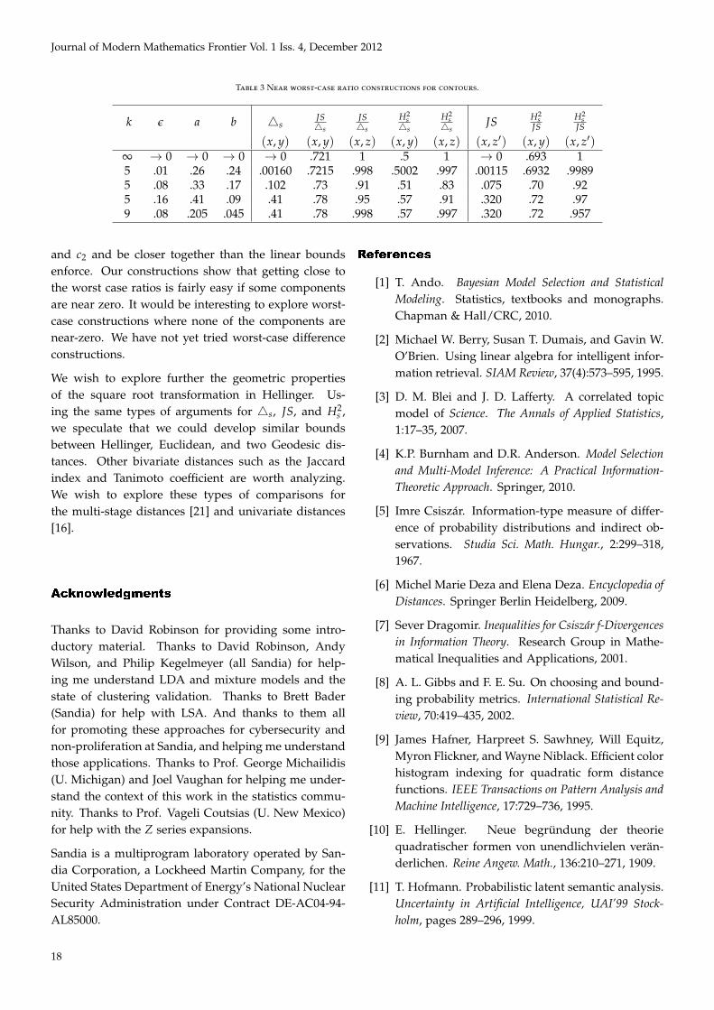
Here we demonstrate where these ratio bounds may benearly achieved. As before, equality is achieved whenall functions are 1, at x · y = 0.
The following construction nearly achieves the ex-tremes of the inequality bounds for a single contour.Let x = (a, a, ...a, b, b, ...b, 0) where a = 1/(k − 1) + ε
and b = 1/(k− 1)− ε. Let y = (b, b, ...b, a, a, ...a, 0) andz = (x1, x2, ...xj, c, 0, 0, ...0, d) where j, c, and d are cho-sen so that D1(x, y) = D1(x, z). Then as k → ∞ andε → 0 we have D2(x, y)/D1(x, y) → the least possibleand D2(x, z)/D1(x, z) → 1. Table 3 illustrates trends.
This example relies on several things; if any of these donot hold, tighter bounds are possible. First, it relies onthe dimension k being large, and (second) the availabil-ity of zero components in x. Third, it relies on xi ≈ yi
and hence (fourth) D1 being small.
However, one can get fairly close to this worst casewithout being very extreme, as observed from the largeflat section of the z-ratio curves in Figure 9, as long aswe keep the availability of zero (or near-zero) compo-nents to provide points where the ratio is near 1.
For example, keeping only the second condition, choos-ing k = 5, ε = 0.08, gives x = (.33, .33, .17, .17, 0),y = (.17, .17, .33, .33, 0), and z = (.33, .33, .042, .128).Here 4s(x, y) = 4s(x, z) = .102 and JS(x, y) =
0.075, JS(x, z) = .094 and H2s (x, y) = .053, H2
s (x, z) =
.085 so JS(x, y)/4s (x, y) = .73 ≈ 0.721, JS(x, z)/4s
(x, z) = .91 ≈ 1, H2s (x, y)/4s (x, y) = .51 ≈ 0.5, and
H2s (x, z)/4s (x, z) = .83 ≈ 1.
Changing z = (.33, .33, .17, .060, .110) gives JS(x, y) =
JS(x, z) = .075 and H2s (x, y) = .053, H2
s (x, z) =
.069 so H2s (x, y)/JS(x, y) = .70 ≈ 0.693, and
H2s (x, z)/JS(x, z) = .92 ≈ 1. Table 3 describes some
other variations we have computed. The last threecolumns describe extreme ratios between Hellinger-squared and Jensen-Shannon, for the same point yand a new point z′ equidistant from x under Jensen-Shannon, z′ : JS(x, y) = JS(x, z′).
Conclusions
We hope that our organization of properties is illu-minating for those using distance functions over mix-ture models, and will inspire further geometric analy-sis. The proofs are detailed so as to be easily repro-ducible, which we thought would be useful given ourattempts to find them in the literature and the difficultyof combining log and square-root functions and variouspowers.
We have given an algebraic and geometric comparisonof the components of 4s, JS, and H2
s . We have factoredthese functions into more easily comparable forms, inthe process illuminating their dependence and behavioron features of the points. We have provided theoreticalbounds on componentwise ratios and differences, andprovided concrete examples that nearly achieve the ra-tio bounds. However, much work remains.
We have provided linear bounds on ratios JS/4s, etc.,but the functional forms suggest it is possible to derivetighter nonlinear bounds. For example, the similarityof contours 4s = c1 and JS = c2 might depend on c1
17
Journal of Modern Mathematics Frontier Vol. 1 Iss. 4, December 2012
Table 3 Near worst-case ratio constructions for contours.
k ε a b 4sJS4s
JS4s
H2s4s
H2s4s
JS H2s
JSH2
sJS
(x, y) (x, y) (x, z) (x, y) (x, z) (x, z′) (x, y) (x, z′)∞ → 0 → 0 → 0 → 0 .721 1 .5 1 → 0 .693 15 .01 .26 .24 .00160 .7215 .998 .5002 .997 .00115 .6932 .99895 .08 .33 .17 .102 .73 .91 .51 .83 .075 .70 .925 .16 .41 .09 .41 .78 .95 .57 .91 .320 .72 .979 .08 .205 .045 .41 .78 .998 .57 .997 .320 .72 .957
and c2 and be closer together than the linear boundsenforce. Our constructions show that getting close tothe worst case ratios is fairly easy if some componentsare near zero. It would be interesting to explore worst-case constructions where none of the components arenear-zero. We have not yet tried worst-case differenceconstructions.
We wish to explore further the geometric propertiesof the square root transformation in Hellinger. Us-ing the same types of arguments for 4s, JS, and H2
s ,we speculate that we could develop similar boundsbetween Hellinger, Euclidean, and two Geodesic dis-tances. Other bivariate distances such as the Jaccardindex and Tanimoto coefficient are worth analyzing.We wish to explore these types of comparisons forthe multi-stage distances [21] and univariate distances[16].
Acknowledgments
Thanks to David Robinson for providing some intro-ductory material. Thanks to David Robinson, AndyWilson, and Philip Kegelmeyer (all Sandia) for help-ing me understand LDA and mixture models and thestate of clustering validation. Thanks to Brett Bader(Sandia) for help with LSA. And thanks to them allfor promoting these approaches for cybersecurity andnon-proliferation at Sandia, and helping me understandthose applications. Thanks to Prof. George Michailidis(U. Michigan) and Joel Vaughan for helping me under-stand the context of this work in the statistics commu-nity. Thanks to Prof. Vageli Coutsias (U. New Mexico)for help with the Z series expansions.
Sandia is a multiprogram laboratory operated by San-dia Corporation, a Lockheed Martin Company, for theUnited States Department of Energy’s National NuclearSecurity Administration under Contract DE-AC04-94-AL85000.
References
[1] T. Ando. Bayesian Model Selection and StatisticalModeling. Statistics, textbooks and monographs.Chapman & Hall/CRC, 2010.
[2] Michael W. Berry, Susan T. Dumais, and Gavin W.O’Brien. Using linear algebra for intelligent infor-mation retrieval. SIAM Review, 37(4):573–595, 1995.
[3] D. M. Blei and J. D. Lafferty. A correlated topicmodel of Science. The Annals of Applied Statistics,1:17–35, 2007.
[4] K.P. Burnham and D.R. Anderson. Model Selectionand Multi-Model Inference: A Practical Information-Theoretic Approach. Springer, 2010.
[5] Imre Csiszár. Information-type measure of differ-ence of probability distributions and indirect ob-servations. Studia Sci. Math. Hungar., 2:299–318,1967.
[6] Michel Marie Deza and Elena Deza. Encyclopedia ofDistances. Springer Berlin Heidelberg, 2009.
[7] Sever Dragomir. Inequalities for Csiszár f-Divergencesin Information Theory. Research Group in Mathe-matical Inequalities and Applications, 2001.
[8] A. L. Gibbs and F. E. Su. On choosing and bound-ing probability metrics. International Statistical Re-view, 70:419–435, 2002.
[9] James Hafner, Harpreet S. Sawhney, Will Equitz,Myron Flickner, and Wayne Niblack. Efficient colorhistogram indexing for quadratic form distancefunctions. IEEE Transactions on Pattern Analysis andMachine Intelligence, 17:729–736, 1995.
[10] E. Hellinger. Neue begründung der theoriequadratischer formen von unendlichvielen verän-derlichen. Reine Angew. Math., 136:210–271, 1909.
[11] T. Hofmann. Probabilistic latent semantic analysis.Uncertainty in Artificial Intelligence, UAI’99 Stock-holm, pages 289–296, 1999.
18
Journal of Modern Mathematics Frontier Vol. 1 Iss. 4, December 2012
[12] K. C. Jain and Amit Srivastava. On symmetricinformation divergence measures of Csiszar’s f-divergence class. Journal of Applied Mathematics,Statistics and Informatics (JAMSI), 3(1):85–99, 2007.
[13] G.G. Judge and R.C. Mittelhammer. An Informa-tion Theoretic Approach to Econometrics. CambridgeUniversity Press, 2011.
[14] S. Kullback and R.A. Leibler. On informationand sufficiency. Annals of Mathematical Statistics,22(1):79–86, 1951.
[15] E. Levina and P. Bickel. The earth mover’s dis-tance is the Mallows distance: some insights fromstatistics. Proceedings. Eighth IEEE International Con-ference on Computer Vision. ICCV 2001., 2:251–256,2001.
[16] Marina Meila. Comparing clusterings by the vari-ation of information. Learning Theory and KernelMachines, pages 173–187, 2003.
[17] Karl Pearson. On the criterion that a given systemof deviations from the probable in the case of acorrelated system of variables is such that it can bereasonably supposed to have arisen from randomsampling. Philosophical Magazine, 50:157–175, 1900.
[18] S. Peleg, M. Werman, and H. Rom. A unifiedapproach to the change of resolution: Space andgray-level. IEEE Trans. Pattern Anal. Mach. Intell.,11(7):739–742, 1989.
[19] David G. Robinson. Statistical language anal-ysis for automatic exfiltration event detection,SAND2010-2179. Technical report, Sandia NationalLaboratories, 2010.
[20] Yossi Rubner, Jan Puzicha, Carlo Tomasi, andJoachim M. Buhmann. Empirical evaluation of dis-similarity measures for color and texture. ComputerVision and Image Understanding, 84:25–43, 2001.
[21] Yossi Rubner, Carlo Tomasi, and Leonidas J.Guibas. The earth mover’s distance as a metricfor image retrieval. Technical report, Stanford Uni-versity, Stanford, CA, USA, 1998.
[22] D. Schnitzer. Dealing with the Music of the World: In-dexing Content-Based Music Similarity Models for FastRetrieval in Massive Databases. CreateSpace, 2012.
[23] Xiaojun Wan. A novel document similarity mea-sure based on earth mover’s distance. Inf. Sci.,177(18):3718–3730, 2007.
[24] Afra Zomorodian and Gunnar Carlsson. Com-puting persistent homology. In SCG ’04: Proceed-ings of the Twentieth Annual Symposium on Compu-tational Geometry, pages 347–356, New York, NY,USA, 2004. ACM.
Data Model and Application Context
One interesting source of mixture models is the analy-sis of a corpus of text documents using statistical tech-niques. For example, one might consider the corpus ofmath and computer science papers from the last fiveyears, and be interested in seeing how well this paper(the one you are reading now!) clusters with the ma-chine learning literature, or whether it is an outlier asthe author suspects.
In order to answer such a question, one selects an ap-propriate model (an art full of choices) and then usesa mathematical computer program to turn documentsinto data points in some space: Latent Dirichlet Alloca-tion and Latent Semantic Analysis are common choices.Next the points are clustered. (In some contexts theoutput of LDA is considered clustered already by thelargest topic component.) But in order to cluster points(i.e. documents), some notion of distance between pointsis required.
However, which of the many distance functions shouldyou choose? Current practice is that the distance func-tion is chosen by some combination of four criteria.First, do you reproduce the ground truth? This is onlypossible if ground truth is available and trustworthy.E.g. you might consider the journal that a paper waspublished in as the ground truth of what cluster it be-longs in. Unfortunately this confounds the choice ofdistance function with the choices of methods and otherparameters. Second, you consider the stability of theoutcome as in cross validation. Are similar clusteringsproduced when some data are withheld, or the distancethreshold is varied, etc.? Third, you pick the distancefunction that has been historically used for your appli-cation domain. Despite the obvious shortcomings, thisfacilitates evaluating new work, and leverages the in-sight your application community has built up aboutyour distance function. Fourth, you pick the distancefunction based on information theory, the idea that thedistance is measuring something relevant such as en-tropy. This often coincides with historical applicationpractice. This paper ignores all of the above (very rea-sonable) criteria, and instead considers complementaryand foundational first-principles geometric and alge-braic comparisons.
19

Journal of Modern Mathematics Frontier Vol. 1 Iss. 4, December 2012
The computational geometry community has not his-torically focused on statistical distances, except for im-age analysis [21]. Even there, the study is usually basedon evaluating the outcome by the four criteria above.
Other Types of Distances
There are other distance types for collections of mixturemodels that are outside the scope of this paper, but areworth mentioning.
Point-to-point distances can be conflated with somenotion of distance (other than orthogonality) betweenthe coordinate axes or histogram bins, called “cross-bin similarity.” This is natural in the setting of LDA,where each coordinate represents a topic, and the top-ics themselves reside as mixture model points in a high-dimensional word space with meaningful distances be-tween topics. The Earth Mover’s Distance has beenused in exactly this way for combining document simi-larity with sub-topic similarity [23]. The Earth Mover’sDistance [18] a.k.a. Mallows Distance [15] forms a cer-tain product of these distances after solving a linearprogram. The Quadratic form [9] is an alternative usinga different product, without the linear program. Rub-ner et al. [20] compares nine distances, including somecross-bin similarities, in the application context of im-age comparisons.
Combining distances also arises in the setting whereeach point represents a structured histogram, humanshave selected the bins, and the meaning of the bins ofthe histogram are more or less related. For example, incybersecurity, one could build a histogram of featuresof packet headers. One might want to assign the bin for“day of the week” to have a smaller distance to the binfor “time of day” than the bin for “packet size.”
Meila Divergence [16] measures the similarity betweenpartitions based on entropy and mutual information.That is, it is useful to compare the quality of differ-ent clusterings, in contrast to whatever distance andmethod was used to create the clusterings in the firstplace.
Univariate measures (i.e. for single points) have theiruses as well. For example in community detection, anentropy measure of a sub-graph may help one decidewhether it is a community or should be further subdi-vided, and it may not matter how the entropy of twodisjoint subgraphs compare.
Model GenerationRecall the problem of determining the relationship ofthis paper (document) to others in a corpus of jour-nal papers (documents). A document is considered tobe composed of a collection of words: a bag of words,where word order and grammar are ignored. Much artis devoted to selecting the words to keep. For example,one might throw away common words like “the.” Onemight retain just the stem of words, obviously help-ful for ignoring tense, but also emphasizing word rootsand meaning by treating “weighting,” “unweighted,”and “weightier,” all as “weight.” The retained wordsin the bag are then weighted to produce entries in adocument-word matrix C. Weighting is also an art, e.g.weights equal to frequency of occurrence are not as dis-tinguishing as weights equal to entropy of occurrence.These approaches have proven very effective, despitethe obvious information loss.
Statistical Model, LDA
Fig. 10 LDA implied Bayesian hierarchical structure. Theta and Phi are
from Dirichlet distributions parameterized by multivariate alpha and
beta: θ ∼ Dir(α), φ ∼ Dir(β). The goal is to discover the unobserved
circled quantities from the observed ones. Figure courtesy of Robinson
[19].
Latent Dirichlet Allocation (LDA) takes this document-word matrix C (corpus) and produces a topic-word ma-trix φ (which we will ignore) and a document-topicmatrix θ (our data); see “Probabilistic Latent Seman-tic Analysis” in Figure 11 and [19]. Each document-column of θ is a mixture of topics, the contribution ofeach topic to that document. The matrix product φθ
gives the probability distribution over the vocabulary.This is in contrast to an approximation of the wordcounts.
LDA assumes a hidden generative model. The topicsare hidden variables. The “true” underlying hiddenmodel for each document is assumed to be a sequenceof topics, of length equal to the number of words in thatdocument. Topics may be repeated in this sequence.Each topic instance in the sequence randomly generatedone of its words and contributed it to the document;
20
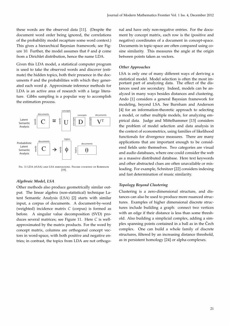
Journal of Modern Mathematics Frontier Vol. 1 Iss. 4, December 2012
these words are the observed data [11]. (Despite thedocument word order being ignored, the correlationsof the probability model recapture some word context.)This gives a hierarchical Bayesian framework; see Fig-ure 10. Further, the model assumes that θ and φ comefrom a Dirichlet distribution, hence the name LDA.
Given this LDA model, a statistical computer programis used to take the observed words and discover (esti-mate) the hidden topics, both their presence in the doc-uments θ and the probabilities with which they gener-ated each word φ. Approximate inference methods forLDA is an active area of research with a large litera-ture. Gibbs sampling is a popular way to accomplishthe estimation process.
documents
wor
ds
documents
wor
ds
wor
ds
topi
cs
topics
documents
wor
ds
conc
epts
concepts
documents
C
C
Uconcepts
conc
epts
D VT
φ θ
=Latent SemanticAnalysis
ProbabilisticLatent
SemanticAnalysis
∼
Fig. 11 LDA (pLSA) and LSA derivations. Figure courtesy of Robinson
[19].
Algebraic Model, LSA
Other methods also produce geometrically similar out-put. The linear algebra (non-statistical) technique La-tent Semantic Analysis (LSA) [2] starts with similarinput, a corpus of documents. A document-by-word(weighted) incidence matrix C (corpus) is formed asbefore. A singular value decomposition (SVD) pro-duces several matrices; see Figure 11. Here C is well-approximated by the matrix products. For the word byconcept matrix, columns are orthogonal concept vec-tors in word-space, with both positive and negative en-tries; in contrast, the topics from LDA are not orthogo-
nal and have only non-negative entries. For the docu-ment by concept matrix, each row is the (positive andnegative) coordinates of a document in concept-space.Documents in topic-space are often compared using co-sine similarity. This measures the angle at the originbetween points taken as vectors.
Other Approaches
LSA is only one of many different ways of deriving astatistical model. Model selection is often the most im-portant part of analyzing data. The effect of the dis-tances used are secondary. Indeed, models can be an-alyzed in many ways besides distances and clustering.Ando [1] considers a general Bayesian framework formodeling, beyond LSA. See Burnham and Anderson[4] for an information-theoretic approach to selectinga model, or rather multiple models, for analyzing em-pirical data. Judge and Mittelhammer [13] considersthe problem of model selection and data analysis inthe context of econometrics, using families of likelihoodfunctionals for divergence measures. There are manyapplications that are important enough to be consid-ered fields unto themselves. Two categories are visualand audio databases, where one could consider the webas a massive distributed database. Here text keywordsand other abstracted clues are often unavailable or mis-leading. For example, Schnitzer [22] considers indexingand fast determination of music similarity.
Topology Beyond Clustering
Clustering is a zero-dimensional structure, and dis-tances can also be used to produce more nuanced struc-tures. Examples of higher dimensional discrete struc-tures include building a graph: connect two verticeswith an edge if their distance is less than some thresh-old. Also building a simplicial complex, adding a sim-plex spanning points contained in a ball as in the Cechcomplex. One can build a whole family of discretestructures, filtered by an increasing distance threshold,as in persistent homology [24] or alpha-complexes.
21