geometric comparison of popular mixture model …samitch/papers/geometric-distances.pdfgeometric...
TRANSCRIPT

Geometric Comparison of Popular Mixture Model Distances
Geometric Comparison of Popular Mixture Model Distances
Scott A. Mitchell [email protected]
Computing Research
Sandia National Laboratories
P.O. Box 5800, MS1316
Albuquerque, NM 87185-1316, USA
Editor:
Abstract
Triangular discrimination, Jensen-Shannon divergence, and the square of the Hellinger distance,are popular distance functions for mixture models, and are known to be similar. Here we expoundupon their equivalence in terms of their functional forms after transformations, factorizations,and series expansions, and in terms of the geometry of their contours. The ratio between thesedistances is nearly flat for modest ratios of point coordinates, up to about 4:1. Beyond thatthe functions increase at different rates. We include derivations of ratio bounds, and some newdifference bounds. We provide some constructions that nearly achieve the worst-cases. These helpus understand when the different functions would give different orderings to the distances betweenpoints.
Keywords: Mixture Models, Geometry, Distance Functions, Theory
1. Introduction
Mixture models are ubiquitous in statistics and their applications. Mixture models express quantitieswhose components are positive and sum to one. They conveniently express a discrete probabilitydistribution for exclusion settings, where probabilities sum to one. They also express fractions ofa whole, e.g. they frequently arise after normalization. They are geometrically equivalent to pointslying on a regular simplex. See Appendix A for how a mixture model arises in one informationapplication.
A distance function measures how close two points are to one another. In clustering applications,points that are close to each other based on this distance are grouped together. Nearest-neighborsoften play a special role. For a given point, different distance functions may give different orderingsto the other points, and different clusters may result.
Triangular discrimination, Jensen-Shannon divergence, and the square of the Hellinger distance,are popular distance functions. There are others, but we focus on these three because they are knownto be similar. The literature and folklore contain some relations, but these provide limited insightfor the following reasons. The prior focus is on the most extreme results, worst case bounds, themaximum and minimum ratio of one distance to another. These are often given as a list of algebraicinequalities, without proof or even hints at reasons why the inequalities hold. We are interestedin understanding which sets of points give rise to these extremes, and what we should expect inintermediate cases. We are interested in the geometry of the mappings underlying the functions,and their series expansions. These provide insight into the form and relation of the functions acrossall cases. Factorizations provides a simplification and parameterization of the bounds. Section 4.7provides some new bounds on the difference between functions, i.e. D1 −D2.
These results provide some underpinnings for answering the question, “In what situations doesit matter which distance function you choose?” using first principles rather than anecdotal casestudies. That is, we explore the class of points for which the different distances would give different
1

Scott A. Mitchell
answers, e.g. to nearest-neighbor queries or constant-value contour constructions. One value of ourexposition is the algebraic decomposition of the functions into products of functions of one variable,always valuable when working in high dimensions. Some of these bounds appear to be well known,but we hope this is a useful geometric description, systematic treatment, and parameterization ofthese bounds. Also we provide proofs from first principles that readers will find easy to reproduce,something that appears to be currently missing in the literature.
2. Model
2.1 Mixture-Model Geometry
1
2T
S+
S
Two-dimensional mixture models T, unit sphere S, and positive part of unit sphere S+
.
Coordinate axis 1 and 2.
x
Point x on T projected to S+
under normalization and square-root.
2xx
x
1
2T
S+
S
Two-dimensional mixture models T, unit sphere S, and positive part of unit sphere S+
.
Coordinate axis 1 and 2.
x
Point x on T projected to S+
under normalization and square-root.
2xx
x
1,0,0 0,1,0
0,0,1
1 2
3
TS+
Figure 1: Left, the domain of mixture models is the simplex T , the unit sphere is S, and the non-negative part of unit sphere is S+. This figure for two-dimensions with coordinate axes 1and 2. Center, point x on T projected to S+ under normalization (Euclidean) and squareroot (Hellinger). Right, three-dimensional simplex T and S+ (cut-away).
Geometrically, mixture model points lie on a regular simplex T ; see Figure 1. Algebraically,these are vectors with positive entries which sum to one. Let K denote the dimension of the model.Let x denote a data point, with xk the kth coordinate of x. Then
T =
x :K∑
k=1
xk = 1, and 1 ≥ xk ≥ 0
.
T is a regular simplex in RK , the convex hull of the elementary vectors ek = {x : xk = 1, xj 6=k =0}, ∀k ∈ [1,K].
For Hellinger and Euclidean (Cosine) distances, we map points from T to the unit K-sphereS, specifically the closed section S+ of it bounded by the positive coordinate planes; see Figure 1.Since zero coordinates map to zero coordinates, all the vertices, edges, etc. of T map to the expectedvertices, edges, etc. of S+. That is, if we treat T and S+ as simplicial complexes, with subsimplicesTI and S+I with xi∈I = 0 for all indicator sets of indices I, then both maps are isomorphisms fromsub-simplex TI to the expected sub-simplex S+I .
Algebraic methods such as non-negative matrix factorization produces output on S+. The rangeof some other algebraic methods, such as LSA after normalization, is all of S. The cosine similaritydistance is naturally defined on all of S.
2

Geometric Comparison of Popular Mixture Model Distances
2.2 Distance Properties
We desire distances D that satisfy these useful properties:
0. Unique Zero: D(x, y) ≥ 0, and D(x, y) = 0 if and only if x = y.
1. Max 1: D ≤ 1 and D(x, y) = 1 for some x, y ∈ T .
2. Symmetry: D(x, y) = D(y, x).
3. Triangle Inequality: D(x, z) ≤ D(x, y) +D(y, z).
4. Orthogonal Max: D(x, y) = 1 if x · y = 0.
(Properties 0–3 are numbered as a reminder to their meaning.) These properties are desired for avariety of practical, theoretical, and historical reasons. Many of our distances satisfy all these exceptfor Triangle Inequality. Properties Unique Zero, Symmetry and Triangle Inequality arerequired for a distance to be a metric. Property Max 1 means we want distances to be bounded; wescale them to have a consistent maximum to facilitate comparisons. This is not required for metrics.Scaled distances are subscripted by s.
Orthogonal Max implies that the distances between points on disjoint sub-simplices of T areall equal. This is desirable from a mixture model perspective because such points are maximallyindependent, hence their distances should be the largest possible and equivalent.
For many ideas that originally emerged without some of these properties, the statistics communityhas developed versions which do. There are several interesting and popular pre-metrics that satisfysome of these. For example, Kullback-Leibler (Kullback and Leibler, 1951) lacks symmetry, butseveral versions of it have been “fixed.”
2.3 Inter-Distance Properties
Two distances D and F have (are)
• Bounded Difference: if c1 ≥ F (x, y)−D(x, y) ≥ 0 for some positive constant c1 < 1.
• Bounded Ratio: if F (x, y) ≥ D(x, y) ≥ c2F (x, y) for some positive constant c2.
• Order Preserving: if D(x, y) < D(x, z) ⇐⇒ F (x, y) < F (x, z).
For our distances, one of them is always greater than the other, so considering the absolute value ofthe difference, i.e. |F (x, y)−D(x, y)|, provides no additional insight.
These properties are a way of relating one function to another. For example, Order Preservingfunctions will produce the same k-nearest neighbor clusterings, provided the analogous distancethresholds are picked. Cosine similarity interprets points as vectors from the origin, and measuresthe cosine of the angle between two of them. If points are first normalized to S, cosine similarity andEuclidean distance are Order Preserving, because the cosine of the angle and the chord lengthbetween the points are both monotonic in the angle.
If D and F satisfy Max 1, then Bounded Ratio implies Bounded Difference with c1 = 1−c2,since F −D = F (1−D/F ) ≤ 1(1− c2). But in the following we often show a smaller constant c1.
2.4 Distance Relation Summary
We define distances 4s, JS, and H2s . We investigate them throughout the rest of the paper.
Figure 2 summarizes their relationships. Motivated by the same desire for a common framework forcomparison, Gibbs and Su (2002) provides a similar diagram.
Here 4s is scaled triangular discrimination, a variant of Chi-squared, χ2. JS is Jensen-Shannon(a.k.a. half the Jeffreys Divergence), a form of Kullback-Leibler. H2
s is scaled and squared Hellinger,
3

Scott A. Mitchell
2ss HJS ≥≥Δ
12
)(⎟⎟⎠
⎞⎜⎜⎝
⎛+−+
yxyxQyx
1112
2
)()(∑
∞
=−+
−
nn
n
n yxyxa
1),max(),min(
2),max(
⎟⎟⎠
⎞⎜⎜⎝
⎛yxyxZyx
12 ),max(
),min(12
),max( ∑∞
=⎟⎟⎠
⎞⎜⎜⎝
⎛−
n
n
n yxyxbyx
Figure 2: Distance metric taxonomy. Given our scaling, the top line shows a strict ordering of thefunction values. Further, equality is achieved only at zero and one and we show non-trivialbounded ratio and difference. The bottom two lines show that each of the three functionscan be factored into those four expressions, but with different Q and Z functions, anddifferent an and bn coefficients.
a variant of scaled Hellinger, Hs, and raw Hellinger, H. The inequalities denote componentwiseinequality, plus bounded ratio and bounded difference. The equations below the box for 4s, JS,and H2
s denote alternative functional forms derived from factorization and series expansions.These satisfy all of our useful properties, except for Triangle Inequality. Raw H does satisfy
Triangle Inequality. Figure 3 illustrates a few interesting examples of distance functions in threedimensions.
These three are relative distances, meaning they depend on the ratio of the pair of points’coordinates. Specifically, we show that each of the 4s, JS, and H2
s distances (generically D) canbe neatly factored into
D(x, y) =
∥∥∥∥p2Q(q)
∥∥∥∥1
=
∥∥∥∥u2Z(z)
∥∥∥∥1
= 1−∥∥∥∥u2W (z)
∥∥∥∥1
.
Here p = x + y is plus, d = x − y is difference and q = d/p is quotient; also u = max(x, y),v = min(x, y), and z = v/u. Of course the Q,Z and W functions are different for each distancefunction D, so we will subscript them by the particular D. Throughout this paper all operations onvectors (e.g. d/p) are applied componentwise. Often the subscripts will be dropped on equations,usually this will still mean that the equality holds componentwise; instead we will explicitly mentionit when equality only holds in the aggregate after taking norms. ‖ · ‖1 denotes the standard L-1vector norm, and is not a componentwise operation; and | · | denotes componentwise absolute value.
Moreover, we will show that all the Q are similar: componentwise
Q(q) =
∞∑n=1
anq2n, 1 ≥ an > 0, an rapidly decreasing, andQ(0) = 0, Q(1) = 1.
All the Z are also similar: componentwise
Z(z) =
∞∑n=2
bn(1− z)n, 1 ≥ bn > 0, bn decreasing, and Z(0) = 1, Z(1) = 0.
Z(z) = 1 + z −W (z), with Z and W monotonic and W (0) = 1,W (1) = 2.
For each of 4s, JS, and H2s , the D, p2Q, and u
2Z functional forms are all componentwise equal; incontrast D = 1 − ‖u2W‖1 only holds in aggregate after taking the 1-norm, i.e. Dk 6= 1 −Wk nor1/K −Wk in general.
4

Geometric Comparison of Popular Mixture Model Distances
In Section 3.3.2 we briefly contrast Hellinger to Eus, the Euclidean distance between mixturemodel points after they have been projected to the unit sphere.
Functions of the form Df (x, y) = ‖xf(x/y)‖1 for convex functions f are known as f-divergences.They were largely developed by Csiszar (Csiszar, 1967). Dragomir (2001) provides many theoremsabout them, including noting that our family of functions are f-divergences. Jain and Srivastava(2007) provides some symmetric variants of f-divergence distances, including our triangular discrim-ination.
In particular, we have componentwise D(x, y) = xD(1, x/y) = yD(y/x, 1), hence Z(z) =D(1, z) = D(z, 1). Similarly we show Q(q) = D(1 + q, 1 − q) = D(1 − q, 1 + q). We provide asimple geometric interpretation of these forms using similar triangles in Section 4.1, Figure 7.
(1,0,0)(0,1,0)
(0,0,1)
(0,0,1)
Distances from (1,0,0)
(0,1,0)
(0,0,1)
(1,0,0)
Distances from (.5,.5,0) Distances
from (.2,.3,.5)
(0,0,1)
(0,1,0)
(1,0,0)
(1,0,0) (0,1,0)
(0,1,0)
(0,0,1)
(1,0,0)
(0,0,1) (1,0,0)
3-dimensional mixture model distances using Euclideanu (yellow + black contours), Hellingers (blue) and JSs (red)
(0,0,1)
(0,1,0)
(1,0,0)
Distances from (.89,.1,.01)
Figure 3: Comparison of Eus, Hellinger, and JSs distances on 3d mixture models. Note the similar-ity between the contour lines for Hs and JSs, and how they contrast with those of Eu inblack. Bottom figures: the red arrow indicates the position of the point (0.89,.1,.01). Notethe steep slope for Hs and JSs as the line (1, 0, 0), (0, 0, 1) is approached, indicated bythe blue and red “walls” on the edges of their graphs, and their contours curving sharplytowards (0.89,.1,.01).
5

Scott A. Mitchell
3. Distance Definitions
3.1 Triangular Discrimination, 4s
The definition of the venerable Chi-Squared Test statistic (Pearson, 1900) is χ2 =∑ (o−e)2
e where ois the observed value and e is the expected value.
Most authors take o and e to be mixture model points, yielding χ2(x, y) = ‖(x− y)2/y‖1. Alter-natively, e could be taken to be the average of all of the points, or the simplex center, which wouldyield a univariate measure.
We fix the asymmetry to obtain the scaled triangular discrimination:
4s =1
2
K∑k=1
(xk − yk)2
xk + yk=
1
2
∥∥∥∥∥ (x− y)2
x+ y
∥∥∥∥∥1
=1
2
∥∥∥∥∥d2p∥∥∥∥∥1
.
Another derivation of 4s is to assume mixture model points are taken from the same population,so the expected value is the average of the two points. That is 4s = χ2(x, (x+y)/2). For continuitythe kth term of the sum is defined to be 0 if xk + yk = 0.
We use this simple measure because it turns out to fit in the same geometric family as Jensen-Shannon and Hellinger-squared.4s obviously satisfies properties Unique Zero and Symmetry. Any term where yk = 0 reduces
to xk, so Max 1 and Orthogonal Max hold.But 4s is too convex, in the sense that 4s(x, y) � 2 4s (x, x/2 + y/2), and does not satisfy
Triangle Inequality even when restricted to mixture models. E.g. x = [1, 0], z = [0, 1] and y =[1/2, 1/2] has 4s(x, y) = 4s(y, z) = 1/3 and 4s(x, z) = 1. Normalizing points so that they lie onthe unit sphere S+ first helps make the function less convex, but not enough: e.g. if y = [1, 1]/
√2
then 4s(x, y) = 0.379.
3.2 Jensen-Shannon Divergence
One information theory approach to distance is based on entropy and divergence. The derivationstarts with the Kullback-Leibler measure, KL, then modifies it for our useful properties, arriving atthe Jensen-Shannon Divergence, JS. This is also known as one-half of the Jeffrey Divergence.
KL(x, y) =∥∥x log2(x/y)
∥∥1
KL is non-symmetric in x and y, which motivates KLsym(x, y) =∥∥x log2(x/y) + y log2(y/x)
∥∥1.
Despite w logw being reasonably well behaved near zero, having independent quantities inside thelog’s means KLsym,k is unbounded for xk = 0 xor yk = 0. Moreover, if xk = 0, it doesn’t matterwhat value yk > 0 has, the k term always contributes the same amount, infinity. Indeed, it doesn’tmatter what any of the other yj 6=k or xj 6=k terms are! To “fix” this, we replace the denominator inthe log’s by the average of x and y:
JS = JSs =1
2
∥∥∥∥x log2
2x
x+ y+ y log2
2y
x+ y
∥∥∥∥1
.
To make JS continuous xk log22xk
xk+yk≡ 0 for xk = 0, since limw→0 w log2 w = 0.
This is a measure of relative distance, the difference between small component values is accen-tuated non-linearly; see Figure 4 left. The constant factors inside the log’s were chosen so thatJSk = xk/2 for yk = 0, which provides Orthogonal Max and Max 1. If yk = xk then log2(1) = 0which verifies Unique Zero. (It may not be obvious that JS ≥ 0, but it is, and can be seen fromsome stronger results we prove later.) Symmetry holds by the symmetry of the functional form.
But JS does not satisfy Triangle Inequality, and is not fixed by normalizing the points to thesphere. This can be verified using the same easy points as for 4s. Indeed, JS is even more convexthan 4s, as amplified in the following section.
6
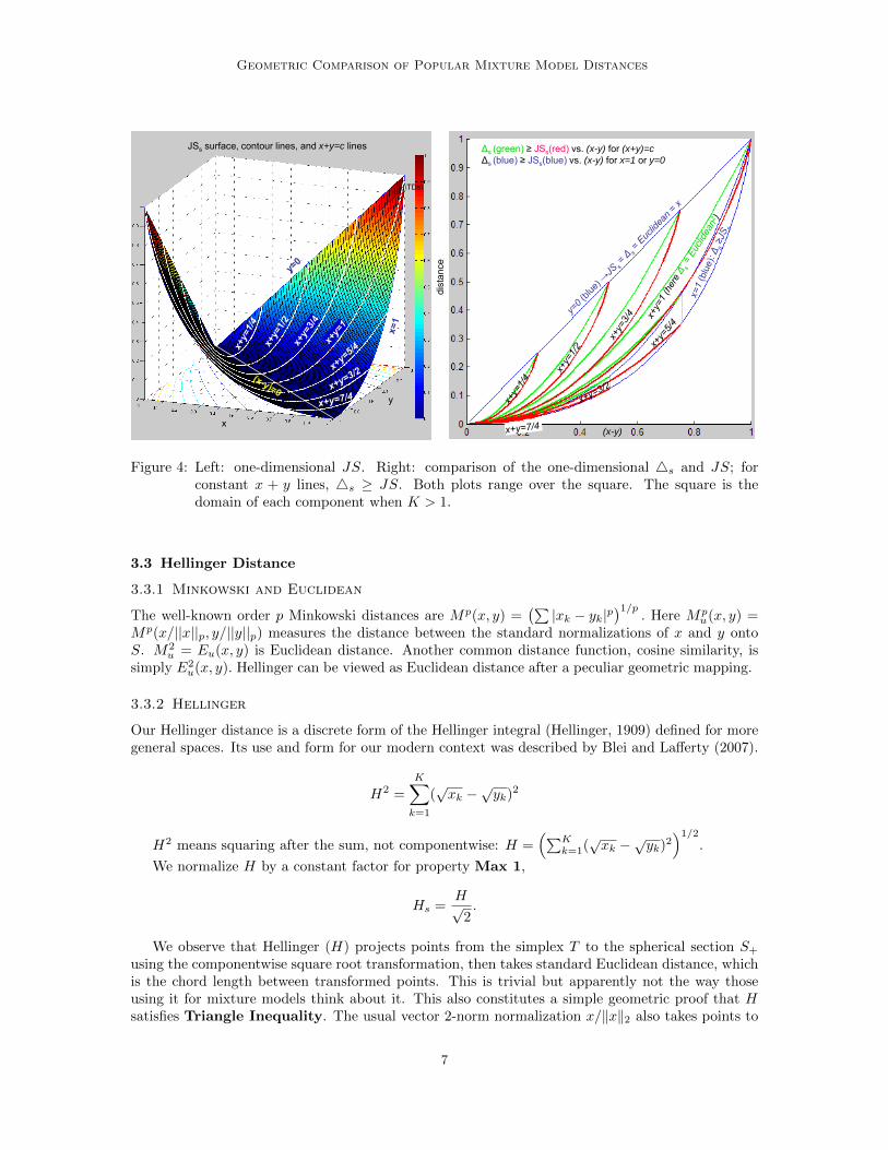
Geometric Comparison of Popular Mixture Model Distances
Δs (green) ≥ JSs(red) vs. (x-y) for (x+y)=cΔs (blue) ≥ JSs(blue) vs. (x-y) for x=1 or y=0
(x-y)di
stan
ce
JSs surface, contour lines, and x+y=c lines
x
y
\TDs\
Figure 4: Left: one-dimensional JS. Right: comparison of the one-dimensional 4s and JS; forconstant x + y lines, 4s ≥ JS. Both plots range over the square. The square is thedomain of each component when K > 1.
3.3 Hellinger Distance
3.3.1 Minkowski and Euclidean
The well-known order p Minkowski distances are Mp(x, y) =(∑|xk − yk|p
)1/p. Here Mp
u(x, y) =Mp(x/||x||p, y/||y||p) measures the distance between the standard normalizations of x and y ontoS. M2
u = Eu(x, y) is Euclidean distance. Another common distance function, cosine similarity, issimply E2
u(x, y). Hellinger can be viewed as Euclidean distance after a peculiar geometric mapping.
3.3.2 Hellinger
Our Hellinger distance is a discrete form of the Hellinger integral (Hellinger, 1909) defined for moregeneral spaces. Its use and form for our modern context was described by Blei and Lafferty (2007).
H2 =
K∑k=1
(√xk −
√yk)2
H2 means squaring after the sum, not componentwise: H =(∑K
k=1(√xk −
√yk)2
)1/2.
We normalize H by a constant factor for property Max 1,
Hs =H√
2.
We observe that Hellinger (H) projects points from the simplex T to the spherical section S+
using the componentwise square root transformation, then takes standard Euclidean distance, whichis the chord length between transformed points. This is trivial but apparently not the way thoseusing it for mixture models think about it. This also constitutes a simple geometric proof that Hsatisfies Triangle Inequality. The usual vector 2-norm normalization x/‖x‖2 also takes points to
7
Scott A. Mitchell
the sphere but is significantly different, e.g. it is a linear scaling of all components. When goingto the sphere, Hellinger expands straight-line-distances near the boundary of T , where ratios ofcomponents are highest, whereas normalization modestly expands straight-line-distances near thecenter of T . Both map the same sub-simplices of T to the obvious subsimplices of S+, and bothmaps agree at sub-simplex centers. Some bounds on the difference of these projections are known.
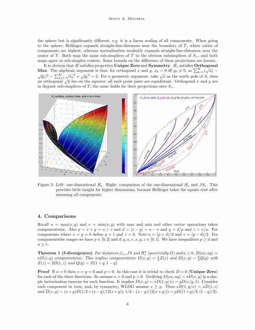
It is obvious that H satisfies properties Unique Zero and Symmetry. Hs satisfies OrthogonalMax. The algebraic argument is that, for orthogonal x and y, xk = 0 iff yk 6= 0, so
∑Kk=1(√xk −√
yk)2 =∑K
k=1
√xk
2 +√yk
2 = 2. For a geometric argument, take√x as the north pole of S, then
an orthogonal√y lies on the equator; all such point pairs are equidistant. Orthogonal x and y are
in disjoint sub-simplices of T ; the same holds for their projections onto S+.
Hs
surface, contour lines, and x+y=c
lines Hs
(blue)
and JSs
(red)
vs. (x-y)
for (x+y)=c, x=1
or y=0
y=0
x=1
y=0
x=1
x+y=
1/4
x+y=
1/2
x+y=
3/4
x+y=
1
x+y=5/4
x+y=3/2
x+y=7/4
x+y=
1
x+y=3/2x+y=
1/2
(x-y)
y
x
Figure 5: Left: one-dimensional Hs. Right: comparison of the one-dimensional Hs and JSs. Thisprovides little insight for higher dimensions, because Hellinger takes the square root aftersumming all components.
4. Comparisons
Recall u = max(x, y) and v = min(x, y) with max and min and other vector operations takencomponentwise. Also p = x + y = u + v and d = |x − y| = u − v and q = d/p and z = v/u. Forcomponents where x = y = 0 define q = 1 and z = 0. Note u = (p + d)/2 and v = (p − d)/2. Forcomponentwise ranges we have p ∈ [0, 2] and d, q, u, v, x, y, z ∈ [0, 1]. We have inequalities p ≥ d andu ≥ v.
Theorem 1 (f-divergences) For distances4s, JS and H2s (generically D) and a ≥ 0, D(ax, ay) =
aD(x, y) componentwise. This implies componentwise D(x, y) = u2Z(z) and D(x, y) = p
2Q(q) withZ(z) = 2D(1, z) and Q(q) = D(1 + q, 1− q).
Proof If u = 0 then x = y = 0 and p = 0. In this case it is trivial to check D = 0 (Unique Zero)for each of the three functions. So assume u > 0 and p > 0. Verifying D(ax, ay) = aD(x, y) is a sim-ple factorization exercise for each function. It implies D(x, y) = xD(1, y/x) = yD(x/y, 1). Considereach component in turn, and, by symmetry, WLOG assume x ≥ y. Then xD(1, y/x) = uD(1, z)and D(x, y) = (x+y)D(1/2+(x−y)/(2(x+y)), 1/2− (x−y)/(2(x+y))) = pD((1+q)/2, (1−q)/2).
8

Geometric Comparison of Popular Mixture Model Distances
Hs2 surface, contour lines, and x+y=c lines
Δs(green) ≥ JSs(red) ≥ H2s (blue) vs. (x-y)
for (x+y)=c, x=1, or y=0
(x-y)
y
x
Figure 6: Left: one-dimensional H2s . Right: comparison of the one-dimensional 4s, JS, and H2
s . InSection 4.1 we show that the family of 4s, JS, H2
s triples of curves are all linear scalings(and truncations) of a single triple of curves, the plots of the Q functions. In Section 4.3we show that straight-lines from the origin to the x = 1 curve (the rightmost-edge of theleft figure) map out the surface. This x = 1 curve is the lower envelop of the curves onthe right, and is the Z function.
For our functions the restriction of the domain to the unit square can be ignored, so we can factorout the 1/2 which provides the compact expression Q(q) = D(1 + q, 1− q).
What this means geometrically is straight-lines from the origin to the x = 1 (or y = 1) curvemap out the surface of the one-dimensional distance functions over the square; see Figure 7. Theslope of each line is related to the value of the Z-function (slope = Z(z)/
√1 + z2) or Q-function
(slope = Q(q)√
2/√
1 + q2).
4.1 Functions of p and q
Here we examine the Q functions for each of4s, JS andH2s . Figure 8 illustrates various relationships
between them.
Theorem 2 (Q-functions) Componentwise
4s =p
2Q4(q) and JS =
p
2QJS(q) andH2
s =p
2QH(q)
whereQ4(q) = q2
QJS(q) =1
2
((1 + q) log2(1 + q) + (1− q) log2(1− q)
)QH(q) = 1−
√1− q2
9
Scott A. Mitchell
JS
u=x=
1 ↔
Z(z)
q = 1 ↔
z = 0
q = 1/3 ↔ z = 1/2q = 0 ↔
z = 1x y
x+y
= 1 ↔
Q(q)
0,0 1,1
1,0
Z(z)
Q(q
)
q=c 1, z=c2
q=1,
z=0
q=0, z=1
p=1
p=1.
5
p= 0
.6
u=1
u=.7u= 0.4
labels are lengths of segments, except points o, o’
geometrically: D( ) = (r / r’) D(o) = (p/1) D(o) = p Q(q)/2
also works for p > 1
2d
2q
22
21
2p
r
r′ 1o′
o
labels are lengths of segments, except points o, o’
geometrically: D( ) = (s / s’) D(o) = (u / 1) D(o) = u/2 Z(z)
z
0
1
1
0
rr′′o
o′′
uv
uv
1
o
o′′o′
2d
2q
22
21
2p
z
1
0
0
zzq
+−
=11
qqz
+−
=11
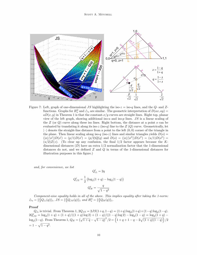
Figure 7: Left, graph of one-dimensional JS highlighting the iso-z = iso-q lines, and the Q- and Z-functions. Graphs for H2
s and4s are similar. The geometric interpretation of D(ax, ay) =aD(x, y) in Theorem 1 is that the constant-x/y curves are straight lines. Right top, planarview of the left graph, showing additional iso-u and iso-p lines. JS is a linear scaling ofthe Z (or Q) curve along these iso lines. Right bottom, the distance at a point o can beevaluated by translating it along its iso-z (iso-q) line to the Z (Q) curve. Geometrically, let| · | denote the straight-line distance from a point to the left (0, 0) corner of the triangle inthe plane. Then linear scaling along iso-q (iso-z) lines and similar triangles yields D(o) =(|o|/|o′|)D(o′) = (p/1)D(o′) = (p/2)Q(q) and D(o) = (|o|/|o′′|)D(o′′) = (u/1)D(o′′) =(u/2)Z(z). (To clear up any confusion, the final 1/2 factor appears because the K-dimensional distances (D) have an extra 1/2 normalization factor that the 1-dimensionaldistances do not, and we defined Z and Q in terms of the 1-dimensional distances forillustration purposes in this figure.)
and, for convenience, we list
Q′4 = 2q
Q′JS =1
2
(log2(1 + q)− log2(1− q)
)Q′H =
q√1− q2
Component-wise equality holds in all of the above. This implies equality after taking the 1-norm:4s = ‖p2Q4(q)‖1, JS = ‖p2QJS(q)‖1 and H2
s = ‖p2QH(q)‖1.
ProofQ4 is trivial. From Theorem 1, 2QJS = 2JS(1+q, 1−q) = (1+q) log2(1+q)+(1−q) log2(1−q).
2Q′JS = log2(1 + q) + (1 + q)/((1 + q) log 2) + (1 − q)/((1 − q) log 2) − log2(1 − q) = log2(1 + q) −log2(1−q). From Theorem 1, QH =
(√1 + q −
√1− q
)2/2 =
(1 + q + 1− q − 2
√(1 + q)(1− q)
)/2
= 1−√
1− q2.
10
Geometric Comparison of Popular Mixture Model Distances
Q functions
q
Q(q
)Δs - Hs
2
(blue)
Difference in Q functions
q
(Q1
–Q
2)
Δs / JS (red)
Ratio of Q functions
q
Q2
/ Q1
Relative difference in Q functions (Q
1–
Q2)
/ (Q
1+
Q2)
q
JS and Hs2 (black)
Hs2
(blue)
JS(red)
Δs(green)
JS / Hs2 (black)
Δs / Hs2 (blue)
Δs - JS(red)
JS - Hs2
(black)
Δs and Hs2 (blue)
Δs and JS (red)
Q functions
q
Q(q
)
Δs - Hs2
(blue)
Difference in Q functions
q
(Q1
–Q
2)
JS / Δs (red)
Ratio of Q functions
q
Q1
/ Q2
Relative difference in Q functions (Q
1–
Q2)
/ (Q
1+
Q2)
q
JS and Hs2 (black)
Hs2
(blue)
JS(red)
Δs(green)
Hs2 / JS (black)
Hs2 / Δs (blue)
Δs - JS(red)
JS - Hs2
(black)
Δs and Hs2 (blue)
Δs and JS (red)
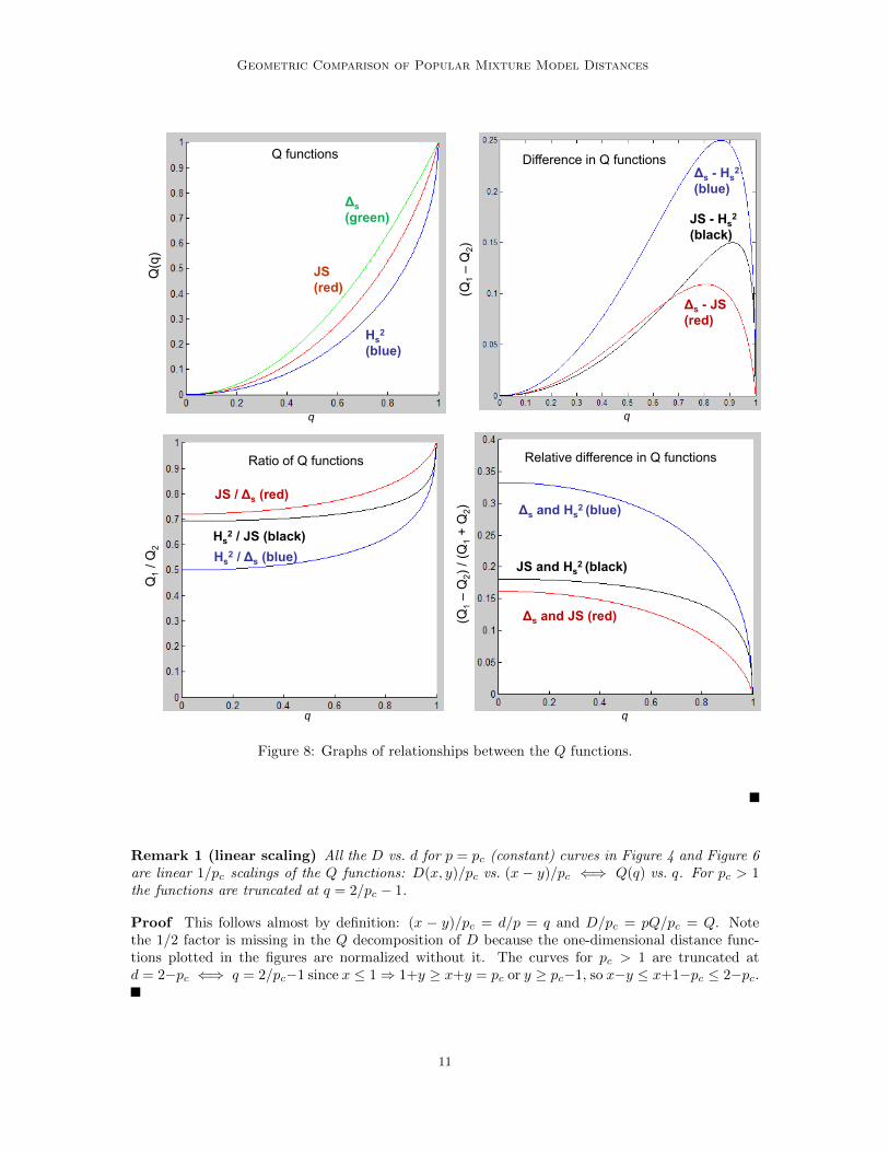
Figure 8: Graphs of relationships between the Q functions.
Remark 1 (linear scaling) All the D vs. d for p = pc (constant) curves in Figure 4 and Figure 6are linear 1/pc scalings of the Q functions: D(x, y)/pc vs. (x − y)/pc ⇐⇒ Q(q) vs. q. For pc > 1the functions are truncated at q = 2/pc − 1.
Proof This follows almost by definition: (x − y)/pc = d/p = q and D/pc = pQ/pc = Q. Notethe 1/2 factor is missing in the Q decomposition of D because the one-dimensional distance func-tions plotted in the figures are normalized without it. The curves for pc > 1 are truncated atd = 2−pc ⇐⇒ q = 2/pc−1 since x ≤ 1⇒ 1+y ≥ x+y = pc or y ≥ pc−1, so x−y ≤ x+1−pc ≤ 2−pc.
11
Scott A. Mitchell
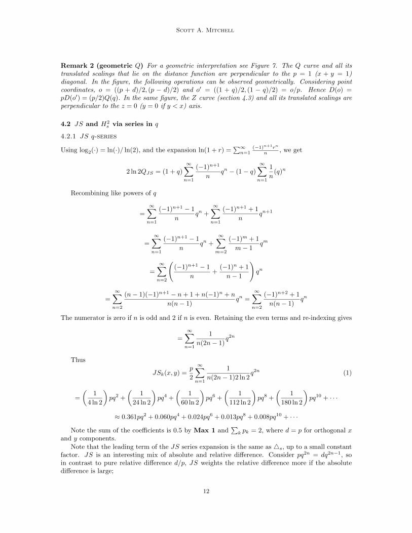
Remark 2 (geometric Q) For a geometric interpretation see Figure 7. The Q curve and all itstranslated scalings that lie on the distance function are perpendicular to the p = 1 (x + y = 1)diagonal. In the figure, the following operations can be observed geometrically. Considering pointcoordinates, o = ((p + d)/2, (p − d)/2) and o′ = ((1 + q)/2, (1 − q)/2) = o/p. Hence D(o) =pD(o′) = (p/2)Q(q). In the same figure, the Z curve (section 4.3) and all its translated scalings areperpendicular to the z = 0 (y = 0 if y < x) axis.
4.2 JS and H2s via series in q
4.2.1 JS q-series
Using log2(·) = ln(·)/ ln(2), and the expansion ln(1 + r) =∑∞
n=1(−1)n+1rn
n , we get
2 ln 2QJS = (1 + q)
∞∑n=1
(−1)n+1
nqn − (1− q)
∞∑n=1
1
n(q)n
Recombining like powers of q
=
∞∑n=1
(−1)n+1 − 1
nqn +
∞∑n=1
(−1)n+1 + 1
nqn+1
=
∞∑n=1
(−1)n+1 − 1
nqn +
∞∑m=2
(−1)m + 1
m− 1qm
=
∞∑n=2
((−1)n+1 − 1
n+
(−1)n + 1
n− 1
)qn
=
∞∑n=2
(n− 1)(−1)n+1 − n+ 1 + n(−1)n + n
n(n− 1)qn =
∞∑n=2
(−1)n+2 + 1
n(n− 1)qn
The numerator is zero if n is odd and 2 if n is even. Retaining the even terms and re-indexing gives
=
∞∑n=1
1
n(2n− 1)q2n
Thus
JSk(x, y) =p
2
∞∑n=1
1
n(2n− 1)2 ln 2q2n (1)
=
(1
4 ln 2
)pq2 +
(1
24 ln 2
)pq4 +
(1
60 ln 2
)pq6 +
(1
112 ln 2
)pq8 +
(1
180 ln 2
)pq10 + · · ·
≈ 0.361pq2 + 0.060pq4 + 0.024pq6 + 0.013pq8 + 0.008pq10 + · · ·
Note the sum of the coefficients is 0.5 by Max 1 and∑
k pk = 2, where d = p for orthogonal xand y components.
Note that the leading term of the JS series expansion is the same as 4s, up to a small constantfactor. JS is an interesting mix of absolute and relative difference. Consider pq2n = dq2n−1, soin contrast to pure relative difference d/p, JS weights the relative difference more if the absolutedifference is large;
12

Geometric Comparison of Popular Mixture Model Distances
4.2.2 H2s q-series
Using the expansion√
1 + r =∑∞
n=0(−1)n(2n)!
(1−2n)(n!)24n rn with r = −q2 gives
QH = 1−∞∑
n=0
(−1)n(2n)!
(1− 2n)(n!)24n(−1)nq2n =
∞∑n=1
(2n)!
(2n− 1)(n!)24nq2n
Therefore componentwise
H2s =
p
2
∞∑n=1
(2n)!
(2n− 1)(n!)24nq2n (2)
=
(1
4
)pq2 +
(1
16
)pq4 +
(1
32
)pq6 +
(5
256
)pq8 +
(7
512
)pq10 + · · ·
≈ 0.2500pq2 + 0.0625pq4 + 0.0312pq6 + 0.0195pq8 + 0.0137pq10 + · · ·
Note the coefficients of the larger powers are bigger than for the JS series, which is illustratedby the larger curvature in Figure 6 right.
4s, JS and H2s have similar behavior, but through different operations and of different order.
4s is a simple ratio of powers, JS uses log2, and H2s uses
√. If yk = 0, then the kth component
of 4s, JS, and H2s are all equal to xk/2. The contours (iso-value lines) for all three have similar
shape. See Figure 3.
4.3 Functions of u and z
Here we describe the Z functional forms for 4s, JS and H2s . We also introduce W (z) functions.
Figure 9 illustrates various relationships between the Z-functions for different distances.
Theorem 3 (Z-functions) Componentwise
4s =u
2Z4(z) and JS =
u
2ZJS(z) andH2
s =u
2ZH(z)
where
Z4(z) =(1− z)2
1 + z= 1 + z − 4z
1 + z
ZJS(z) = 1 + z − (1 + z) log2(1 + z) + z log2 z
ZH(z) = 1 + z − 2√z
and for convenience we list
Z ′4 = 1− 4
(1 + z)2=
(z + 3)(z − 1)
(1 + z)2
Z ′JS = 1− log2(1 + z) + log2(z) = 1− log2(1 + z−1)
Z ′H = 1− 1√z
As for the Q functions, all of the above holds componentwise and implies equality after taking1-norms.
13
Scott A. Mitchell
Z functions
z
Z(z)
Relative difference in Z functions (Z
1–
Z 2) /
(Z1
+ Z 2
)
Δs and JS (red)
Δs – JS(red)
Difference in Z functions
z
(Z1
–Z 2
)
z
JS / Δs (red)
Ratio of Z functions
Z 1/ Z
2
related byq = (1-z)/(1+z)p=(u/2)(1+z)
Δs - Hs2
(blue)
JS - Hs2
(black)
Hs2
(blue)
JS(red)
Δs(green)
Hs2 / JS (black)
Hs2 / Δs (blue) JS and Hs
2 (black)
Δs and Hs2 (blue)
z
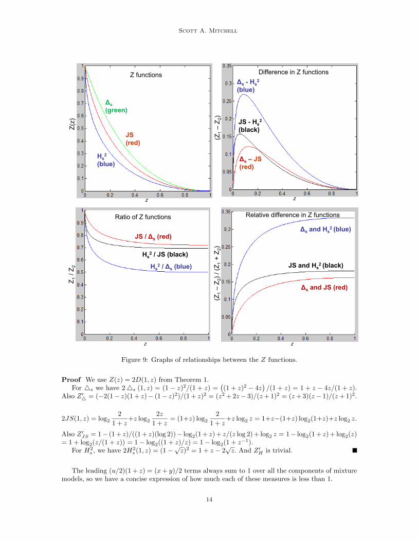
Figure 9: Graphs of relationships between the Z functions.
Proof We use Z(z) = 2D(1, z) from Theorem 1.For 4s we have 24s (1, z) = (1 − z)2/(1 + z) =
((1 + z)2 − 4z
)/(1 + z) = 1 + z − 4z/(1 + z).
Also Z ′4 = (−2(1− z)(1 + z)− (1− z)2)/(1 + z)2 = (z2 + 2z− 3)/(z+ 1)2 = (z+ 3)(z− 1)/(z+ 1)2.
2JS(1, z) = log2
2
1 + z+z log2
2z
1 + z= (1+z) log2
2
1 + z+z log2 z = 1+z−(1+z) log2(1+z)+z log2 z.
Also Z ′JS = 1− (1 + z)/((1 + z)(log 2))− log2(1 + z) + z/(z log 2) + log2 z = 1− log2(1 + z) + log2(z)= 1 + log2(z/(1 + z)) = 1− log2((1 + z)/z) = 1− log2(1 + z−1).
For H2s , we have 2H2
s (1, z) = (1−√z)2 = 1 + z − 2
√z. And Z ′H is trivial.
The leading (u/2)(1 + z) = (x+ y)/2 terms always sum to 1 over all the components of mixturemodels, so we have a concise expression of how much each of these measures is less than 1.
14

Geometric Comparison of Popular Mixture Model Distances
Corollary 4
4s = 1− ‖u2W4(z)‖1 = 1− ‖u
2
4z
1 + z‖1
JS = 1− ‖u2WJS(z)‖1 = 1− ‖u
2(z log2 z − (1 + z) log2(1 + z))‖1
H2s = 1− ‖u
2WH(z)‖1 = 1− ‖u
2(2√z)‖1
The leftmost equality is not componentwise equality. E.g. H2sk 6= 1/k − uk
√zk in general.
Proof In this proof we use subscripts k to emphasize that keeping track of individual com-ponents is important. ‖u2Z(z)‖1 =
∑Kk=1 |
uk
2 (1 + zk −W (zk))|. We first note that 1 + zk ≥W (zk) ≥ 0 so we can remove the absolute value sign. The argument for this is that each com-ponent of the original distance functions is non-negative (since the distance functions are dis-tances over all of RK
+ and not just mixture models) and equal to the Z functions. Each of theW are non-negative. Thus we may drop the absolute values and separate the sum into twogiving ‖u2Z(z)‖1 =
∑Kk=1
uk
2 (1 + zk) −∑K
k=1W (zk). The first sum is 1 because it is merely∑Kk=1 (uk + vk)/2 =
∑Kk=1 (xk + yk)/2 and our domain is mixture models.
4.4 4s, JS and H2s via series in z
Here we provide series expansions for our functions in z, about the point z = 1. For each we definer = 1 − z, and each series contains integer powers of r starting with 2. We make use of 1 − r = z,2− r = z + 1, and 1 ≥ r ≥ 0.
4.4.1 4s z-series
Z4 =(1− z)2
1 + z= r2
(1
2− r
)=r2
2
(1
1− r/2
)=
∞∑n=0
rn+2
2n+1=
∞∑n=2
rn
2n−1
Thus
4s(x, y) = u
∞∑n=2
rn
2n(3)
=
(1
4
)ur2 +
(1
8
)ur3 +
(1
16
)ur4 +
(1
32
)ur5 +
(1
64
)ur6 + · · ·
= 0.25ur2 + 0.125ur3 + 0.0625ur4 + 0.03125ur5 + 0.015625ur6 + · · ·
4.4.2 JS z-series
ZJS has two log terms:
z log z = (1− r) log2(1− r) = −1− rln 2
∞∑n=1
rn
nand
(1 + z) log(1 + z) = (2− r) log2(2− r) =(2− r)
ln 2(ln 2 + ln(1− r/2)) = 2− r +
2− rln 2
ln(1− r/2)
where ln(1− r/2) = −∞∑
n=1
rn
n2n.
15
Scott A. Mitchell
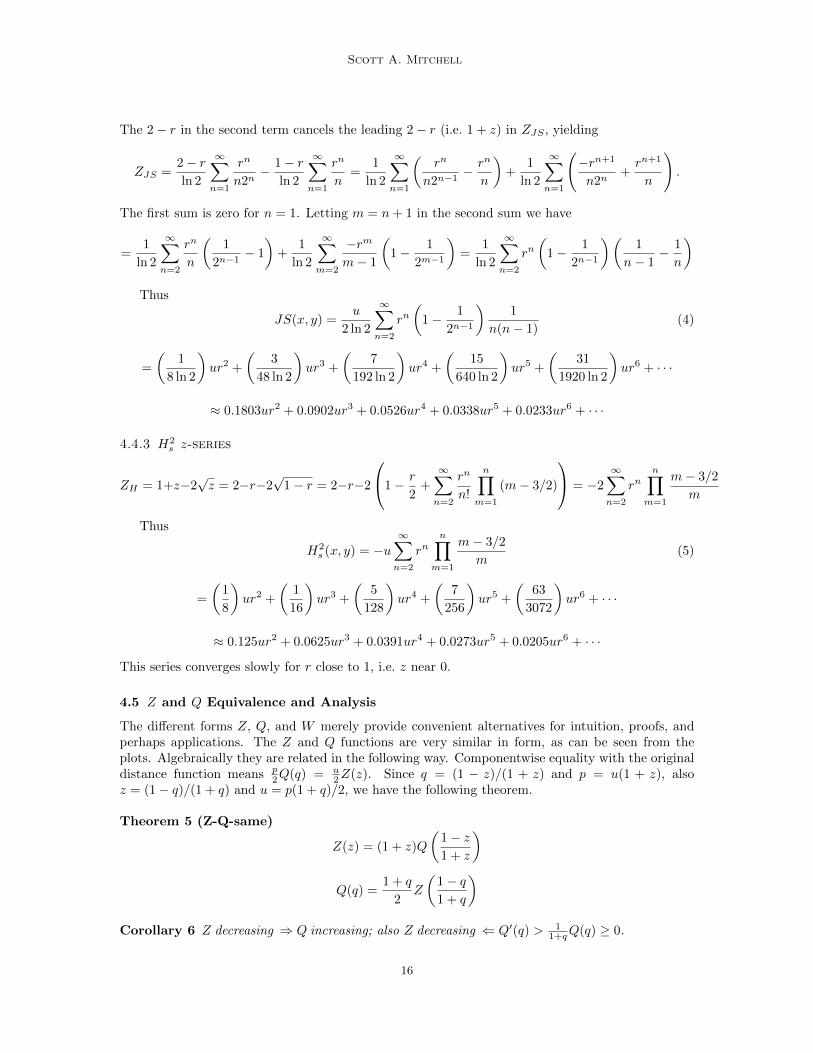
The 2− r in the second term cancels the leading 2− r (i.e. 1 + z) in ZJS , yielding
ZJS =2− rln 2
∞∑n=1
rn
n2n− 1− r
ln 2
∞∑n=1
rn
n=
1
ln 2
∞∑n=1
(rn
n2n−1− rn
n
)+
1
ln 2
∞∑n=1
(−rn+1
n2n+rn+1
n
).
The first sum is zero for n = 1. Letting m = n+ 1 in the second sum we have
=1
ln 2
∞∑n=2
rn
n
(1
2n−1− 1
)+
1
ln 2
∞∑m=2
−rm
m− 1
(1− 1
2m−1
)=
1
ln 2
∞∑n=2
rn(
1− 1
2n−1
)(1
n− 1− 1
n
)Thus
JS(x, y) =u
2 ln 2
∞∑n=2
rn(
1− 1
2n−1
)1
n(n− 1)(4)
=
(1
8 ln 2
)ur2 +
(3
48 ln 2
)ur3 +
(7
192 ln 2
)ur4 +
(15
640 ln 2
)ur5 +
(31
1920 ln 2
)ur6 + · · ·
≈ 0.1803ur2 + 0.0902ur3 + 0.0526ur4 + 0.0338ur5 + 0.0233ur6 + · · ·
4.4.3 H2s z-series
ZH = 1+z−2√z = 2−r−2
√1− r = 2−r−2
1− r
2+
∞∑n=2
rn
n!
n∏m=1
(m− 3/2)
= −2
∞∑n=2
rnn∏
m=1
m− 3/2
m
Thus
H2s (x, y) = −u
∞∑n=2
rnn∏
m=1
m− 3/2
m(5)
=
(1
8
)ur2 +
(1
16
)ur3 +
(5
128
)ur4 +
(7
256
)ur5 +
(63
3072
)ur6 + · · ·
≈ 0.125ur2 + 0.0625ur3 + 0.0391ur4 + 0.0273ur5 + 0.0205ur6 + · · ·
This series converges slowly for r close to 1, i.e. z near 0.
4.5 Z and Q Equivalence and Analysis
The different forms Z, Q, and W merely provide convenient alternatives for intuition, proofs, andperhaps applications. The Z and Q functions are very similar in form, as can be seen from theplots. Algebraically they are related in the following way. Componentwise equality with the originaldistance function means p
2Q(q) = u2Z(z). Since q = (1 − z)/(1 + z) and p = u(1 + z), also
z = (1− q)/(1 + q) and u = p(1 + q)/2, we have the following theorem.
Theorem 5 (Z-Q-same)
Z(z) = (1 + z)Q
(1− z1 + z
)
Q(q) =1 + q
2Z
(1− q1 + q
)Corollary 6 Z decreasing ⇒ Q increasing; also Z decreasing ⇐ Q′(q) > 1
1+qQ(q) ≥ 0.
16

Geometric Comparison of Popular Mixture Model Distances
Proof Z decreasing means ∀z1 < z2, Z(z1) > Z(z2). Since Z(z) = (1 + z)Q((1 − z)/(1 + z)) wehave
Q
(1− z11 + z1
)>
1 + z21 + z1
Q
(1− z21 + z2
)> Q
(1− z21 + z2
)where q1 = 1−z1
1+z1> 1−z2
1+z2= q2. Since the mapping between z and q is a continuous isomorphism
this inequality holds for arbitrary q1 > q2. For the other direction, Z decreasing ⇐⇒ Q(q1) >1+z21+z1
Q(q2) = 1+q11+q2
Q(q2). We manipulate this inequality to get it into derivative form,
Q(q1)−Q(q2)
q1 − q2>
(1 + q11 + q2
− 1
)Q(q2)/(q1 − q2) =
(q1 − q21 + q2
)Q(q2)/(q1 − q2) =
1
1 + q2Q(q2).
This holds always if it holds in the limit as q1 → q2, or Q′(q) > 11+qQ(q).
The stronger requirement for Q′ is necessary; e.g. Q = 1+ q/2 implies Z = (1+z)(1+(1−z)/(2(1+z))) = 3/2 + z/2, so here is an example where both Q and Z are increasing. Geometrically whatis happening is that a constant z (or q) ray from the origin first intersects the p = 1 line, then theu = 1 line. Recall D is rising linearly along this ray. For smaller values of q, the p and u linesare farther apart, so D increases more. For example, a flat Q(q) = 1 function implies an increasingZ(z) = 1 + z function.
Theorem 5 and Corollary 6 hold generically for functions with D(ax, ay) = aD(x, y). We nowturn to our particular functions, and show that the decreasing/increasing conditions hold in the half-open interval q ∈ (0, 1] (or z ∈ [0, 1) ), and they are flat at the excluded end point, i.e. Q′(0) = 0and Z ′(1) = 0.
Theorem 7 (Z-decreasing) Z4(z), ZJS(z), and ZH(z) are all strictly decreasing in [0, 1), withzero derivative at z = 1. Note Z ′4(0) = −3, but Z ′JS(0) = −∞ and Z ′H(0) = −∞.
Proof We can check Z ′ < 0 and the values at 0 and 1 directly from the formulas: Z ′4 = (z+3)(z−1)(1+z)2 ,
all factors positive except z−1; Z ′JS = 1− log2(1+z−1) < 0 ⇐⇒ 2 < 1+z−1; and Z ′H = 1−z−1/2.All these check out for 0 ≤ z < 1.
Corollary 8 (Q-increasing) Q4(z), QJS(z), and QH(z) are all strictly increasing in (0, 1], withzero derivative at q = 0. Note Q′4(1) = 2, but Q′JS(1) =∞ and Q′H(1) =∞.
Proof Increasing in (0, 1] follows from Corollary 6. Derivative values at 0 and 1 can be checked
using Q′4 = 2q. 2Q′JS = log2(1 + q)− log2(1− q), and log2(1− q) < 0 for q > 0. Q′H = q/√
1− q2.
For our three functions, a more complicated but straight-forward alternative is to show Q isincreasing then check the stronger derivative conditions from Corollary 6.
Theorem 9 (Q-increasing-alt) Q4(z), QJS(z), and QH(z) are all strictly increasing in (0, 1],with zero derivative at q = 0. Note Q′4(1) = 2, but Q′JS(1) =∞ and Q′H(1) =∞.
Proof Positive derivatives follow directly from the formulas. Q′4 = 2q. 2Q′JS = log2(1 + q) −log2(1− q)/2, and log2(1− q) < 0 for q > 0. Q′H = q/
√1− q2.
Corollary 10 (Z-decreasing-alt) Z4(z), ZJS(z), and ZH(z) are all strictly decreasing in [0, 1),with zero derivative at z = 1. Note Z ′4(0) = −3, but Z ′JS(0) = −∞ and Z ′H(0) = −∞.
17

Scott A. Mitchell
Proof Relying on Theorem 9 we check the conditions of Corollary 6. Recall Q4 = q2 and Q′4 = 2q.
Then Q′4 > Q4/(1 + q) ⇐⇒ 2q > q2/(1 + q) ⇐⇒ 2q(1 + q) > q2 ⇐⇒ q 6= 0 and 2 > q.
Recall QJS =((1 + q) log2(1 + q) + (1− q) log2(1− q)
)/2 and Q′JS = (log2(1 + q)− log2(1− q))/2.
Then Q′JS > QJS/(1 + q) ⇐⇒ log2(1 + q) − log2(1 − q) > log2(1 + q) + 1−q1+q log2(1 − q) ⇐⇒
0 >(
1−q1+q + 1
)log2(1 − q). The first factor is positive and the second is negative for q < 1. Recall
QH(q) = 1 −√
1− q2 and Q′H = q/√
1− q2. Then Q′H > QH/(1 + q) ⇐⇒ q(1 + q) > (1 −√1− q2)
√1− q2 =
√1− q2 − 1 + q2 ⇐⇒ 1 + q >
√1− q2, which is true for q > 0 since the left
side is increasing and the right is decreasing.
Values at 0 and 1 can be checked by recalling Z ′4 = (z+3)(z−1)(z+1)2 , Z ′JS = 1 − log2(1 + z−1), and
Z ′H = 1− z−1/2.
Theorem 11 Z1
Z2decreasing ⇐⇒ Q1
Q2increasing. Moreover maxZ1/Z2 = maxQ1/Q2 and minZ1/Z2 =
minQ1/Q2
Proof Componentwise equality implies D1
D2= Z1
Z2(z) = Q1
Q2
(q = 1−z
1+z
)and max and min are pre-
served at z = 0 and z = 1 (where q = 1 and q = 0).
We next describe some bounds limiting how much these functions vary from one another. Thenwe give some examples where these bounds are nearly achieved.
4.6 Ratios of 4s, JS and H2s
We start with describing linear bounds between the functions. Tighter bounds apply in a varietyof situations. Many of these linear bounds are already known. For example the following lowerbounds are stated in Jain and Srivastava (2007) without reference or proof. We hope providingstraightforward descriptions and simple proofs here are helpful. In addition, the parameterizationof the ratios by q and z, their monotonicity in these parameters, and geometrically describing theircurves appears novel. Figure 10 summarizes the results of this section.
Q∗ q∗ Z∗ z∗
H2s /4s 1/2 = .500 0 1/2 = .500 1
JS/4s 1/2 log 2 > .721 0 1/2 log 2 > .721 1H2
s /JS log 2 > .693 0 log 2 > .693 1max is 1 at q = 1 and z = 0
Figure 10: Q∗ and Z∗ are the infimums of ratios between Q and Z functions, and q∗ and z∗ are thelimit points where this is achieved. These results are exact.
Bounds on the ratio of Q (or Z) functions implies bounds on the ratio of actual distance functions
D. If 1 ≥ Q1/Q2 ≥ a componentwise, then 1 ≥ maxkD1,k
D2,k≥ ‖D1‖1‖D2‖1 ≥ mink
D1,k
D2,k= a.
Theorem 12 (Ratio bounds JS/4s, H2s /4s, and H2
s /JS)
1 ≥ H2s
4s≥ 0.5
1 ≥ JS
4s≥ 1
2 log 2, note 1/2 log 2 > 0.721.
18
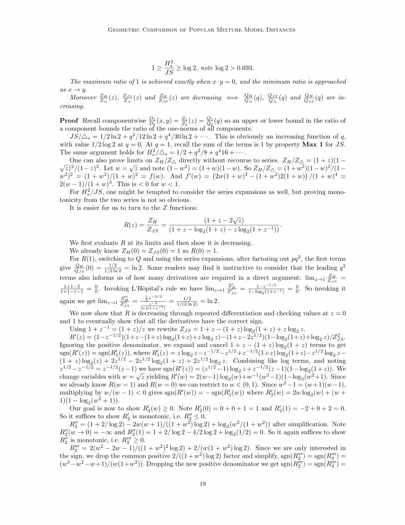
Geometric Comparison of Popular Mixture Model Distances
1 ≥ H2s
JS≥ log 2, note log 2 > 0.693.
The maximum ratio of 1 is achieved exactly when x ·y = 0, and the minimum ratio is approachedas x→ y.
Moreover ZH
Z4(z), ZJS
Z4(z) and ZH
ZJS(z) are decreasing ⇐⇒ QH
Q4(q), QJS
Q4(q) and QH
QJS(q) are in-
creasing.
Proof Recall componentwise D1
D2(x, y) = Z1
Z2(z) = Q1
Q2(q) so an upper or lower bound in the ratio of
a component bounds the ratio of the one-norms of all components.JS/4s = 1/2 ln 2 + q2/12 ln 2 + q4/30 ln 2 + · · · . This is obviously an increasing function of q,
with value 1/2 log 2 at q = 0. At q = 1, recall the sum of the terms is 1 by property Max 1 for JS.The same argument holds for H2
s /4s = 1/2 + q2/8 + q416 + · · · .One can also prove limits on ZH/Z4 directly without recourse to series. ZH/Z4 = (1 + z)(1−√
z)2/(1− z)2. Let w =√z and note (1−w2) = (1 +w)(1−w). So ZH/Z4 = (1 +w2)(1−w)2/(1−
w2)2 = (1 + w2)/(1 + w)2 = f(w). And f ′(w) =(2w(1 + w)2 − (1 + w2)2(1 + w)
)/(1 + w)4 =
2(w − 1)/(1 + w)3. This is < 0 for w < 1.For H2
s /JS, one might be tempted to consider the series expansions as well, but proving mono-tonicity from the two series is not so obvious.
It is easier for us to turn to the Z functions:
R(z) =ZH
ZJS=
(1 + z − 2√z)
(1 + z − log2(1 + z)− z log2(1 + z−1)).
We first evaluate R at its limits and then show it is decreasing.We already know ZH(0) = ZJS(0) = 1 so R(0) = 1.For R(1), switching to Q and using the series expansions, after factoring out pq2, the first terms
give QH
QJS(0) = 1/2
1/2 ln 2 = ln 2. Some readers may find it instructive to consider that the leading q2
terms also informs us of how many derivatives are required in a direct argument: limz→1ZH
ZJS=
1+1−21+1−1−1 = 0
0 . Invoking L’Hopital’s rule we have limz→1Z′HZ′JS
= 1−z−1/2
1−log2(1+z−1) = 00 . So invoking it
again we get limz→1Z′′HZ′′JS
=12 z−3/2
z−2
ln 2(1+z−1)
= 1/21/(2 ln 2) = ln 2.
We now show that R is decreasing through repeated differentiation and checking values at z = 0and 1 to eventually show that all the derivatives have the correct sign.
Using 1 + z−1 = (1 + z)/z we rewrite ZJS = 1 + z − (1 + z) log2(1 + z) + z log2 z.R′(z) = (1−z−1/2)(1+z−(1+z) log2(1+z)+z log2 z)−(1+z−2z1/2)(1−log2(1+z)+log2 z)/Z
2JS .
Ignoring the positive denominator, we expand and cancel 1 + z − (1 + z) log2(1 + z) terms to getsgn(R′(z)) = sgn(R′1(z)), where R′1(z) = z log2 z−z−1/2−z1/2+z−1/2(1+z) log2(1+z)−z1/2 log2 z−(1 + z) log2(z) + 2z1/2 − 2z1/2 log2(1 + z) + 2z1/2 log2 z. Combining like log terms, and notingz1/2−z−1/2 = z−1/2(z−1) we have sgn(R′(z)) = (z1/2−1) log2 z+z−1/2(z−1)(1− log2(1+z)). Wechange variables with w =
√z yielding R′(w) = 2(w−1) log2(w)+w−1(w2−1)(1−log2(w2+1). Since
we already know R(w = 1) and R(w = 0) we can restrict to w ∈ (0, 1). Since w2−1 = (w+1)(w−1),multiplying by w/(w − 1) < 0 gives sgn(R′(w)) = − sgn(R′2(w)) where R′2(w) = 2w log2(w) + (w +1)(1− log2(w2 + 1)).
Our goal is now to show R′2(w) ≥ 0. Note R′2(0) = 0 + 0 + 1 = 1 and R′2(1) = −2 + 0 + 2 = 0.So it suffices to show R′2 is monotonic, i.e. R′′2 ≤ 0.
R′′2 = (1 + 2/ log 2) − 2w(w + 1)/((1 + w2) log 2) + log2(w2/(1 + w2)) after simplification. NoteR′′2 (w → 0) = −∞ and R′′2 (1) = 1 + 2/ log 2− 4/2 log 2 + log2(1/2) = 0. So it again suffices to showR′′2 is monotonic, i.e. R′′′2 ≥ 0.
R′′′2 = 2(w2 − 2w − 1)/((1 + w2)2 log 2) + 2/(w(1 + w2) log 2). Since we are only interested inthe sign, we drop the common positive 2/((1 +w2) log 2) factor and simplify, sgn(R′′′2 ) = sgn(R′′′3 ) =(w3−w2−w+1)/(w(1+w2)). Dropping the new positive denominator we get sgn(R′′′2 ) = sgn(R′′′4 ) =
19
Scott A. Mitchell
w3 −w2 −w+ 1 = (1−w)(1−w2) ≥ 0, which was the goal. Going back up the chain of derivativesshows that each is monotonic and always has the correct sign.
Note that the relative difference bounds and curves in Figure 9 and Figure 8 follows directlyfrom the ratio bounds.
4.7 Differences between 4s, JS and H2s
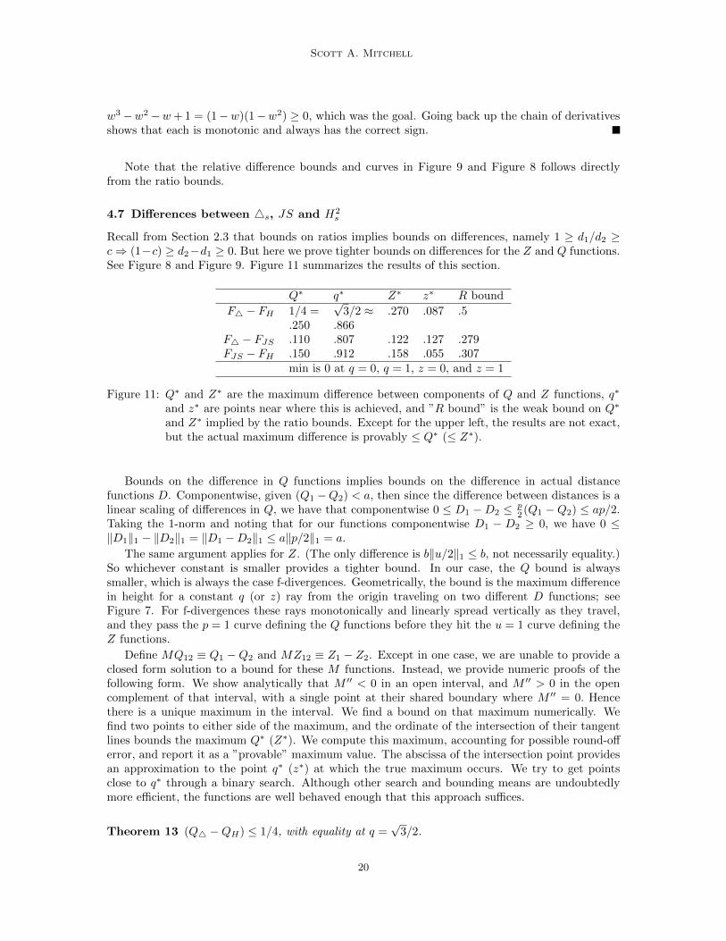
Recall from Section 2.3 that bounds on ratios implies bounds on differences, namely 1 ≥ d1/d2 ≥c⇒ (1−c) ≥ d2−d1 ≥ 0. But here we prove tighter bounds on differences for the Z and Q functions.See Figure 8 and Figure 9. Figure 11 summarizes the results of this section.
Q∗ q∗ Z∗ z∗ R bound
F4 − FH 1/4 =√
3/2 ≈ .270 .087 .5.250 .866
F4 − FJS .110 .807 .122 .127 .279FJS − FH .150 .912 .158 .055 .307
min is 0 at q = 0, q = 1, z = 0, and z = 1
Figure 11: Q∗ and Z∗ are the maximum difference between components of Q and Z functions, q∗
and z∗ are points near where this is achieved, and ”R bound” is the weak bound on Q∗
and Z∗ implied by the ratio bounds. Except for the upper left, the results are not exact,but the actual maximum difference is provably ≤ Q∗ (≤ Z∗).
Bounds on the difference in Q functions implies bounds on the difference in actual distancefunctions D. Componentwise, given (Q1 −Q2) < a, then since the difference between distances is alinear scaling of differences in Q, we have that componentwise 0 ≤ D1 −D2 ≤ p
2 (Q1 −Q2) ≤ ap/2.Taking the 1-norm and noting that for our functions componentwise D1 − D2 ≥ 0, we have 0 ≤‖D1‖1 − ‖D2‖1 = ‖D1 −D2‖1 ≤ a‖p/2‖1 = a.
The same argument applies for Z. (The only difference is b‖u/2‖1 ≤ b, not necessarily equality.)So whichever constant is smaller provides a tighter bound. In our case, the Q bound is alwayssmaller, which is always the case f-divergences. Geometrically, the bound is the maximum differencein height for a constant q (or z) ray from the origin traveling on two different D functions; seeFigure 7. For f-divergences these rays monotonically and linearly spread vertically as they travel,and they pass the p = 1 curve defining the Q functions before they hit the u = 1 curve defining theZ functions.
Define MQ12 ≡ Q1 −Q2 and MZ12 ≡ Z1 − Z2. Except in one case, we are unable to provide aclosed form solution to a bound for these M functions. Instead, we provide numeric proofs of thefollowing form. We show analytically that M ′′ < 0 in an open interval, and M ′′ > 0 in the opencomplement of that interval, with a single point at their shared boundary where M ′′ = 0. Hencethere is a unique maximum in the interval. We find a bound on that maximum numerically. Wefind two points to either side of the maximum, and the ordinate of the intersection of their tangentlines bounds the maximum Q∗ (Z∗). We compute this maximum, accounting for possible round-offerror, and report it as a ”provable” maximum value. The abscissa of the intersection point providesan approximation to the point q∗ (z∗) at which the true maximum occurs. We try to get pointsclose to q∗ through a binary search. Although other search and bounding means are undoubtedlymore efficient, the functions are well behaved enough that this approach suffices.
Theorem 13 (Q4 −QH) ≤ 1/4, with equality at q =√
3/2.
20
Geometric Comparison of Popular Mixture Model Distances
Proof MQ4H = q2 − 1 +√
1− q2 =√
1− q2(1 −√
1− q2). Let w =√
1− q2, we haveMQ4H = w(1− w) and MQ′4H = 1− 2w. The maximum occurs at w = 1/2 ⇐⇒ q =
√3/2 and
has value 1/4.
Lemma 14 (Q4 −QJS)′′ < 0 for q ∈ (q0, 1) and > 0 for q ∈ (0, q0) with q0 ≈ 0.53.
Proof MQ′4J = 2q − (log2(1 + q)− log2(1− q))/2. MQ′′4J = 2− (1/(1 + q) + 1/(1− q))/(2 log 2).
Therefore MQ′′4J < 0 ⇐⇒ 4 log 2 < 1/(1+q)+1/(1−q) = 2/(1−q2) ⇐⇒ q > (1−1/2 log 2)1/2 =q0 ≈ 0.53.
Lemma 15 (QJS −QH)′′ < 0 for q ∈ (q0, 1) and > 0 for q ∈ (0, q0) with q0 ≈ 0.72.
Proof MQ′JH = (log2(1+q)−log2(1−q))/2−q/√
1− q2. MQ′′JH = (1/(1+q)+1/(1−q))/(2 log 2)−(1− q2)3/2 = (1− q2)−1/ log 2− (1− q2)3/2. Therefore MQ′′JH < 0 ⇐⇒
√1− q2 < log 2 ⇐⇒ q >√
1− log2 2 = q0 ≈ 0.72.
Lemma 16 (Z4 − ZH)′′ < 0 for z ∈ (0, z0) and > 0 for z ∈ (z0, 1) with z0 ≈ 0.24.
Proof MZ ′4H = −4/(1 + z)2 + z−1/2. MZ ′′4H = 8/(1 + z)3 − z−3/2/2. Therefore sgn(MZ ′′4H) <
0 ⇐⇒ 16z3/2 < (1 + z)3 ⇐⇒ 2 3√
2√z < 1 + z. Letting w =
√z and solving via the quadratic
formula we have ⇐⇒ w < 3√
2−√
3√
4− 1⇐ z < 0.24.
Lemma 17 (Z4 − ZJS)′′ < 0 for z ∈ (0, z0) and > 0 for z ∈ (z0, 1) with z0 ≈ 0.31.
Proof MZ4J ′ = −4/(1+z)2+log2(1+z−1) and MZ4J ′′ = 8/(1+z)3−1/(z(z+1) log 2). ThereforeMZ4J ′′ < 0 ⇐⇒ z2+(2−8 log 2)z+1 > 0. Solving via the quadratic formula with b = (2−8 log 2)
we have ⇐⇒ z < b/−√b2/4− 1 = z0 ≈ 0.31
Lemma 18 (ZJS − ZH)′′ < 0 for z ∈ (0, z0) and > 0 for z ∈ (z0, 1) with z0 ≈ 0.16.
ProofFrom Theorem 3 we have MZJH = (ZJS − ZH) = − log2(1 + z) − z log2(1 + z−1) + 2
√z and
MZ ′JH(z) = − log2(1 + z−1) + z−1/2.Log functions (base 2 and of 1 + z) can cross square-root functions multiple times, so it is very
helpful to recourse to MZ ′′JH to avoid these difficulties.MZ ′′JH = 1
z(1+z) log 2 −1
2z3/2 . Note 1z(1+z) log 2 −
12z3/2 > 0 ⇐⇒ 1
z(1+z) log 2 > 12z3/2 ⇐⇒
z(1 + z) log 2 < 2z3/2 ⇐⇒ (1 + z) log 2 < 2z1/2. Since z > 0, we may square both sides, ⇐⇒(1 + z)2 < 4
log2 2z ⇐⇒ z2 + 2z− 4
log2 2z+ 1 < 0. Note sgn(f ′′) = sgn(−z2 + 2( 2
log2 2−1)z−1). Using
the quadratic formula the zeros are 2c− 1± 2√c2 − c where c = 1/ ln2 2 = {z0, z1} ≈ {0.162, 6.163}.
Thus MZJH has a single inflection point in (0, 1) at z0. It is easy to verify numerically thatMZ ′′JH(z : z < z0) < 0 and MZ ′′JH(z : 1 ≥ z > z0) > 0.
21

Scott A. Mitchell
4.8 Contours of 4s, JS and H2s
4.8.1 Not Order Preserving Examples.
Measures 4s, JS, H2s (hence Hs) are not order preserving, yet their contours (constant-value sets)
are similar.
Examples of order being switched can be generated by exploiting the different curvatures inFigure 3 bottom or the different coefficients in the series expansions. For x = [0.89, 0.10, 0.01],y = [0.9, 0, 0.1], and z = [0.65, 0.35, 0], we have (4s(x, y) = 0.087) < (4s(x, z) = 0.093) but(JS(x, y) = 0.081) > (JS(x, z) = 0.072) and (H2
s (x, y) = 0.073) > (H2s (x, z) = 0.052). Changing
z to [0.6, 0.4, 0], we have (JS(x, y) = 0.081) < (JS(x, z) = 0.095) but (H2s (x, y) = 0.073) >
(H2s (x, z) = 0.069).
Recall none of 4s, JS, or H2s obey the triangle inequality.
4.8.2 Worst-Case Contour Construction
Here we demonstrate where these ratio bounds may be nearly achieved. As before, equality isachieved when all functions are 1, at x · y = 0.
The following construction nearly achieves the extremes of the inequality bounds for a singlecontour. Let x = (a, a, ...a, b, b, ...b, 0) where a = 1/(k − 1) + ε and b = 1/(k − 1) − ε. Lety = (b, b, ...b, a, a, ...a, 0) and z = (x1, x2, ...xj , c, 0, 0, ...0, d) where j, c, and d are chosen so thatD1(x, y) = D1(x, z). Then as k →∞ and ε→ 0 we have D2(x, y)/D1(x, y)→ the least possible andD2(x, z)/D1(x, z)→ 1. Figure 12 illustrates trends. This example relies on several things; if any ofthese do not hold, tighter bounds are possible. First, it relies on the dimension k being large, and(second) the availability of zero components in x. Third, it relies on xi ≈ yi and hence (fourth) D1
being small.
However, one can get fairly close to this worst case without being very extreme, as observed fromthe large flat section of the z-ratio curves in Figure 9, as long as we keep the availability of zero (ornear-zero) components to provide points where the ratio is near 1.
k ε a b 4sJS4s
JS4s
H2s
4s
H2s
4sJS
H2s
JSH2
s
JS
(x, y) (x, y) (x, z) (x, y) (x, z) (x, z′) (x, y) (x, z′)∞ → 0 → 0 → 0 → 0 .721 1 .5 1 → 0 .693 15 .01 .26 .24 .00160 .7215 .998 .5002 .997 .00115 .6932 .99895 .08 .33 .17 .102 .73 .91 .51 .83 .075 .70 .925 .16 .41 .09 .41 .78 .95 .57 .91 .320 .72 .979 .08 .205 .045 .41 .78 .998 .57 .997 .320 .72 .957
Figure 12: Near worst-case ratio constructions for contours.
For example, keeping only the second condition, choosing k = 5, ε = 0.08, gives x = (.33, .33, .17, .17, 0),y = (.17, .17, .33, .33, 0), and z = (.33, .33, .042, .128). Here 4s(x, y) = 4s(x, z) = .102 andJS(x, y) = 0.075, JS(x, z) = .094 and H2
s (x, y) = .053, H2s (x, z) = .085 so JS(x, y)/ 4s (x, y) =
.73 ≈ 0.721, JS(x, z)/4s (x, z) = .91 ≈ 1, H2s (x, y)/4s (x, y) = .51 ≈ 0.5, and H2
s (x, z)/4s (x, z) =.83 ≈ 1.
Changing z = (.33, .33, .17, .060, .110) gives JS(x, y) = JS(x, z) = .075 andH2s (x, y) = .053, H2
s (x, z) =.069 so H2
s (x, y)/JS(x, y) = .70 ≈ 0.693, and H2s (x, z)/JS(x, z) = .92 ≈ 1. Figure 12 describes
some other variations we have computed. The last three columns describe extreme ratios betweenHellinger-squared and Jensen-Shannon, for the same point y and a new point z′ equidistant from xunder Jensen-Shannon, z′ : JS(x, y) = JS(x, z′).
22
Geometric Comparison of Popular Mixture Model Distances
5. Conclusions
We hope that our organization of properties is illuminating for those using distance functions overmixture models, and will inspire further geometric analysis. The proofs are detailed so as to be easilyreproducible, which we thought would be useful given our attempts to find them in the literatureand the difficulty of combining log and square-root functions and various powers.
We have given an algebraic and geometric comparison of the components of 4s, JS, and H2s .
We have factored these functions into more easily comparable forms, in the process illuminatingtheir dependence and behavior on features of the points. We have provided theoretical bounds oncomponentwise ratios and differences, and provided concrete examples that nearly achieve the ratiobounds. However, much work remains.
We have provided linear bounds on ratios JS/4s, etc., but the functional forms suggest it ispossible to derive tighter nonlinear bounds. For example, the similarity of contours 4s = c1 andJS = c2 might depend on c1 and c2 and be closer together than the linear bounds enforce. Ourconstructions show that getting close to the worst case ratios is fairly easy if some components arenear zero. It would be interesting to explore worst-case constructions where none of the componentsare near-zero. We have not yet tried worst-case difference constructions.
We wish to explore further the geometric properties of the square root transformation in Hellinger.Using the same types of arguments for 4s, JS, and H2
s , we speculate that we could develop similarbounds between Hellinger, Euclidean, and two Geodesic distances. Other bivariate distances such asthe Jaccard index and Tanimoto coefficient are worth analyzing. We wish to explore these types ofcomparisons for the multi-stage distances (e.g. Rubner et al. (1998)) and univariate distances (e.g.Meila (2003)).
Acknowledgments
Thanks to David Robinson for providing some introductory material. Thanks to David Robinson,Andy Wilson, and Philip Kegelmeyer (all Sandia) for helping me understand LDA and mixturemodels and the state of clustering validation. Thanks to Brett Bader (Sandia) for help with LSA.And thanks to them all for promoting these approaches for cybersecurity and non-proliferation atSandia, and helping me understand those applications. Thanks to Prof. George Michailidis (U.Michigan) and Joel Vaughan for helping me understand the context of this work in the statisticscommunity. Thanks to Prof. Vageli Coutsias (U. New Mexico) for help with the Z series expansions.
Sandia is a multiprogram laboratory operated by Sandia Corporation, a Lockheed Martin Com-pany, for the United States Department of Energy’s National Nuclear Security Administration underContract DE-AC04-94-AL85000.
References
Peter Barnum. Similarity and difference: Advanced perception course presentation. http://www.
cs.cmu.edu/~efros/courses/AP06/.../06-07-presentation.ppt, 2006.
Michael W. Berry, Susan T. Dumais, and Gavin W. O’Brien. Using linear algebra for intelligentinformation retrieval. SIAM Review, 37(4):573–595, 1995. doi: 10.1137/1037127. URL http:
//link.aip.org/link/?SIR/37/573/1.
D. M. Blei and J. D. Lafferty. A correlated topic model of Science. The Annals of Applied Statistics,1:17–35, 2007.
Imre Csiszar. Information-type measure of difference of probability distributions and indirect obser-vations. Studia Sci. Math. Hungar., 2:299–318, 1967.
23

Scott A. Mitchell
Sever Dragomir. Inequalities for Csiszar f-Divergences in Information Theory. Research Group inMathematical Inequalities and Applications, 2001.
A. L. Gibbs and F. E. Su. On choosing and bounding probability metrics. International StatisticalReview, 70:419–435, 2002. doi: 10.1111/j.1751-5823.2002.tb00178.x.
James Hafner, Harpreet S. Sawhney, Will Equitz, Myron Flickner, and Wayne Niblack. Efficient colorhistogram indexing for quadratic form distance functions. IEEE Transactions on Pattern Analysisand Machine Intelligence, 17:729–736, 1995. ISSN 0162-8828. doi: http://doi.ieeecomputersociety.org/10.1109/34.391417.
E. Hellinger. Neue begrndung der theorie quadratischer formen von unendlichvielen vernderlichen.Reine Angew. Math., 136:210–271, 1909.
T. Hofmann. Probabilistic latent semantic analysis. Uncertainty in Artificial Intelligence, UAI’99Stockholm, pages 289–296, 1999.
K. C. Jain and Amit Srivastava. On symmetric information divergence measures of Csiszar’s f-divergence class. Journal of Applied Mathematics, Statistics and Informatics (JAMSI), 3(1):85–99, 2007.
S. Kullback and R.A. Leibler. On information and sufficiency. Annals of Mathematical Statistics,22(1):79–86, 1951. doi: http://dx.doi.org/10.1214/aoms/1177729694.
E. Levina and P. Bickel. The earth mover’s distance is the Mallows distance: some insights fromstatistics. Proceedings. Eighth IEEE International Conference on Computer Vision. ICCV 2001.,2:251–256, 2001.
Marina Meila. Comparing clusterings by the variation of information. Learning Theory and KernelMachines, pages 173–187, 2003.
Karl Pearson. On the criterion that a given system of deviations from the probable in the case ofa correlated system of variables is such that it can be reasonably supposed to have arisen fromrandom sampling. Philosophical Magazine, 50:157–175, 1900.
S. Peleg, M. Werman, and H. Rom. A unified approach to the change of resolution: Space andgray-level. IEEE Trans. Pattern Anal. Mach. Intell., 11(7):739–742, 1989. ISSN 0162-8828. doi:http://dx.doi.org/10.1109/34.192468.
David G. Robinson. Statistical language analysis for automatic exfiltration event detection,SAND2010-2179. Technical report, Sandia National Laboratories, 2010.
Yossi Rubner, Carlo Tomasi, and Leonidas J. Guibas. The earth mover’s distance as a metric forimage retrieval. Technical report, Stanford University, Stanford, CA, USA, 1998.
Yossi Rubner, Jan Puzicha, Carlo Tomasi, and Joachim M. Buhmann. Empirical evaluation ofdissimilarity measures for color and texture. Computer Vision and Image Understanding, 84:25–43, 2001. doi: 10.1006/cviu.2001.0934. URL http://www.idealibrary.com.
Xiaojun Wan. A novel document similarity measure based on earth mover’s distance. Inf. Sci., 177(18):3718–3730, 2007. ISSN 0020-0255. doi: http://dx.doi.org/10.1016/j.ins.2007.02.045.
Afra Zomorodian and Gunnar Carlsson. Computing persistent homology. In SCG ’04: Proceedingsof the Twentieth Annual Symposium on Computational Geometry, pages 347–356, New York, NY,USA, 2004. ACM. ISBN 1-58113-885-7. doi: http://doi.acm.org/10.1145/997817.997870.
24

Geometric Comparison of Popular Mixture Model Distances
Appendix A. Data Model and Application Context
One interesting source of mixture models is the analysis of a corpus of text documents using statisticaltechniques. For example, one might consider the corpus of math and computer science papers fromthe last five years, and be interested in seeing how well this paper (the one you are reading now!)clusters with the machine learning literature, or whether it is an outlier as the author suspects.
In order to answer such a question, one selects an appropriate model (an art full of choices) andthen uses a mathematical computer program to turn documents into data points in some space:Latent Dirichlet Allocation and Latent Semantic Analysis are common choices. Next the points areclustered. (In some contexts the output of LDA is considered clustered already by the largest topiccomponent.) But in order to cluster points (i.e. documents), some notion of distance between pointsis required.
However, which of the many distance functions should you choose? Current practice is thatthe distance function is chosen by some combination of four criteria. First, do you reproduce theground truth? This is only possible if ground truth is available and trustworthy. E.g. you mightconsider the journal that a paper was published in as the ground truth of what cluster it belongsin. Unfortunately this confounds the choice of distance function with the choices of methods andother parameters. Second, you consider the stability of the outcome as in cross validation. Aresimilar clusterings produced when some data are withheld, or the distance threshold is varied, etc.?Third, you pick the distance function that has been historically used for your application domain.Despite the obvious shortcomings, this facilitates evaluating new work, and leverages the insight yourapplication community has built up about your distance function. Fourth, you pick the distancefunction based on information theory, the idea that the distance is measuring something relevantsuch as entropy. This often coincides with historical application practice. This paper ignores all ofthe above (very reasonable) criteria, and instead considers complementary and foundational first-principles geometric and algebraic comparisons.
The computational geometry community has not historically focused on statistical distances,except for image analysis (Rubner et al., 1998). Even there, the study is usually based on evaluatingthe outcome as described above by the four criteria.
A.1 Other Uses of Distances
Clustering is a zero-dimensional structure, and distances can also be used to produce more nuancedstructures. Examples of higher dimensional discrete structures include building a graph: connecttwo vertices with an edge if their distance is less than some threshold. Also building a simplicialcomplex, adding a simplex spanning points contained in a ball as in the Cech complex. One can builda whole family of discrete structures, filtered by an increasing distance threshold, as in persistenthomology (Zomorodian and Carlsson, 2004) or alpha-complexes.
A.2 Other Types of Distances
There are other distance types for collections of mixture models that are outside the scope of thispaper, but are worth mentioning.
Point-to-point distances can be conflated with some notion of distance (other than orthogonality)between the coordinate axes or histogram bins, called “cross-bin similarity.” This is natural in thesetting of LDA, where each coordinate represents a topic, and the topics themselves reside as mixturemodel points in a high-dimensional word space with meaningful distances between topics. Wan(2007) has used the Earth Mover’s Distance in exactly this way for combining document similaritywith sub-topic similarity. The Earth Mover’s Distance (Peleg et al., 1989) a.k.a. Mallows Distance(Levina and Bickel, 2001) forms a certain product of these distances after solving a linear program.The Quadratic form (Hafner et al., 1995) is an alternative using a different product, without the
25

Scott A. Mitchell
linear program. Rubner et al. (2001) compares nine distances, including some cross-bin similarities,in the application context of image comparisons; Barnum (2006) provides a nice slide summary.
Combining distances also arises in the setting where each point represents a structured histogram,humans have selected the bins, and the meaning of the bins of the histogram are more or less related.For example, in cybersecurity, one could build a histogram of features of packet headers. One mightwant to assign the bin for “day of the week” to have a smaller distance to the bin for “time of day”than the bin for “packet size.”
Meila Divergence (Meila, 2003) measures the similarity between partitions based on entropy andmutual information. That is, it is useful to compare the quality of different clusterings, in contrastto whatever distance and method was used to create the clusterings in the first place.
Univariate measures (i.e. for single points) have their uses as well. For example in communitydetection, an entropy measure of a sub-graph may help one decide whether it is a community orshould be further subdivided, and it may not matter how the entropy of two disjoint subgraphscompare.
A.3 Model Generation
Recall the problem of determining the relationship of this paper (document) to others in a corpus ofjournal papers (documents). A document is considered to be composed of a collection of words: abag of words, where word order and grammar are ignored. Much art is devoted to selecting the wordsto keep. For example, one might throw away common words like “the.” One might retain just thestem of words, obviously helpful for ignoring tense, but also emphasizing word roots and meaningby treating “weighting,” “unweighted,” and “weightier,” all as “weight.” The retained words in thebag are then weighted to produce entries in a document-word matrix C. Weighting is also an art,e.g. weights equal to frequency of occurrence are not as distinguishing as weights equal to entropyof occurrence. These approaches have proven very effective, despite the obvious information loss.
A.4 Statistical Model, LDA
Figure 13: LDA implied Bayesian hierarchical structure. Theta and Phi are from Dirichlet distribu-tions parameterized by multivariate alpha and beta: θ ∼ Dir(α), φ ∼ Dir(β). The goalis to discover the unobserved circled quantities from the observed ones. Figure courtesyof Robinson (2010).
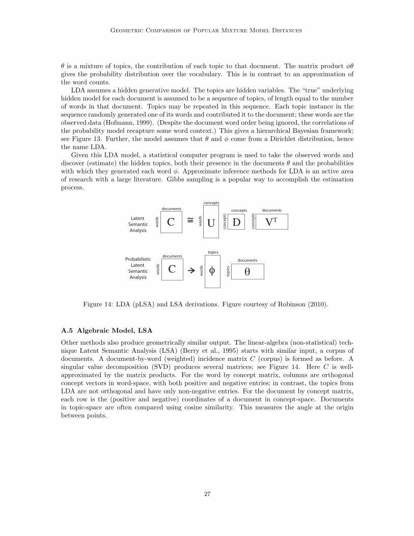
Latent Dirichlet Allocation (LDA) takes this document-word matrix C (corpus) and produces atopic-word matrix φ (which we will ignore) and a document-topic matrix θ (our data); see “Prob-abilistic Latent Semantic Analysis” in Figure 14 and Robinson (2010). Each document-column of
26
Geometric Comparison of Popular Mixture Model Distances
θ is a mixture of topics, the contribution of each topic to that document. The matrix product φθgives the probability distribution over the vocabulary. This is in contrast to an approximation ofthe word counts.
LDA assumes a hidden generative model. The topics are hidden variables. The “true” underlyinghidden model for each document is assumed to be a sequence of topics, of length equal to the numberof words in that document. Topics may be repeated in this sequence. Each topic instance in thesequence randomly generated one of its words and contributed it to the document; these words are theobserved data (Hofmann, 1999). (Despite the document word order being ignored, the correlations ofthe probability model recapture some word context.) This gives a hierarchical Bayesian framework;see Figure 13. Further, the model assumes that θ and φ come from a Dirichlet distribution, hencethe name LDA.
Given this LDA model, a statistical computer program is used to take the observed words anddiscover (estimate) the hidden topics, both their presence in the documents θ and the probabilitieswith which they generated each word φ. Approximate inference methods for LDA is an active areaof research with a large literature. Gibbs sampling is a popular way to accomplish the estimationprocess.
documents
wor
ds
documents
wor
ds
wor
ds
topi
cs
topics
documents
wor
ds
conc
epts
concepts
documents
C
C
Uconcepts
conc
epts
D VT
φ θ
=Latent SemanticAnalysis
ProbabilisticLatent
SemanticAnalysis
∼
Figure 14: LDA (pLSA) and LSA derivations. Figure courtesy of Robinson (2010).
A.5 Algebraic Model, LSA
Other methods also produce geometrically similar output. The linear-algebra (non-statistical) tech-nique Latent Semantic Analysis (LSA) (Berry et al., 1995) starts with similar input, a corpus ofdocuments. A document-by-word (weighted) incidence matrix C (corpus) is formed as before. Asingular value decomposition (SVD) produces several matrices; see Figure 14. Here C is well-approximated by the matrix products. For the word by concept matrix, columns are orthogonalconcept vectors in word-space, with both positive and negative entries; in contrast, the topics fromLDA are not orthogonal and have only non-negative entries. For the document by concept matrix,each row is the (positive and negative) coordinates of a document in concept-space. Documentsin topic-space are often compared using cosine similarity. This measures the angle at the originbetween points.
27