Generation of Counter-Circulating Vortex Linesin a Bose-Einstein Condensate

Thomas K. Langin

Advisor: Professor David S. HallMay 5, 2011

Submitted to theDepartment of Physics of Amherst College

in partial fulfilment of therequirements for the degree ofBachelors of Arts with honors

c© 2011 Thomas K. Langin

Abstract

The intriguing properties of superfluids, such as inviscid flow and the quan-tization of vorticity, have fascinated physicists for nearly a century. Interest hasrecently centered on the dynamics of interactions between vortex-antivortexpairs in superfluids, since these interactions are central to the physics of quan-tum turbulence. Dilute-gas Bose-Einstein condensates (BECs) provide a cleansystem with which we may obtain a better understanding of the dynamicsof these interactions. In this thesis, we present observations of dilute-gasBECs containing two, three, and four counter-circulating vortex lines. Wealso observe possible vortex recombination and/or pair annihilation events.To generate counter-circulating vortices, we make novel use of the ability togenerate vortices of known circulation and the ability to radially translatevortices though exchange of angular momentum between the condensate anda rotating thermal cloud. Further exploration of the mechanisms of vortexgeneration and manipulation will help generate additional counter-circulatingstates of interest, such as stable vortex dipoles and tripoles, as well as conclu-sively identifying reconnection and annihilation events.

Acknowledgments

First thanks go out to my advisor, David Hall. His willingness to let me seek

out my own topics for research helped lead me to the fascinating subject of

quantum turbulence, a subject which I am considering pursuing further once

I leave the confines of Amherst College. Professor Hall’s constant enthusiasm

for experimental physics is truly inspiring, and I encourage every student con-

sidering experimental physics as a possible career path to consider working

in his lab for a summer/interterm/semester. There’s always something to do,

and, even if that something seems like least interesting thing in the world, his

enthusiasm will get you excited about it. Also, without his timely and metic-

ulous editing, this thesis would certainly be a lot less readable. So, anyone

reading this should thank him too!

Second thanks go out to fellow workers in Professor Hall’s lab, both past

and present. In particular, I’d like to thank Daniel Freilich, Emine Altuntas,

and Aftaab Dewan. I learned a lot by working with Daniel during interterm

my junior year, both about the apparatus and about what being a senior thesis

writer was all about (occasionally lots of work...but a great payoff!). Working

with Aftaab over this past summer was a real treat. He rewrote the condensate

fitting program so that it could fit an arbitrary number of vortices. He also was

i

(almost) always down for a good game of Halo, which greatly enhanced the

summer @ Amherst experience. Last but not least, Emine has been a great lab

buddy. Her constant focus and determination to get to the bottom of things

really helped put me on the right track, both during our work together over

the summer and during our more individual work during the academic year.

So thanks for putting up with my shenanigans Emine!

I’ve also got to thank the rest of the class of 2011 physics majors. From

the all night/day I-Lab sessions to the fun times at the hbar and everything

in between, I cannot imagine going through Amherst with a better group of

kids. Special thanks go to Andrew Eddins, whose willingness to have ‘thesis

conversations’ (not the scary kind!) even when he had millions of other things

on his plate (i.e., all the time) was truly admirable. Additional thanks go out

to the physics faculty at Amherst, the interest that each one of you has in

your students’ future is unbelievable at times.

The bros of Taplin 101 were instrumental in the completion of this thesis.

Without you guys to occasionally distract me with a game of midnight soccer,

strikers, or a late night diner run, I may have gone crazy during the past few

months.

Most importantly, thank you Mom, Dad, and Kim. Without your uncon-

ditional support, I wouldn’t have made it as far as I have. You guys mean the

world to me.

This research has been supported by the National Science Foundation

through grant PHY-0855475.

ii

Contents

1 Introduction 11.1 What is a BEC? . . . . . . . . . . . . . . . . . . . . . . . . . . 31.2 Quantized Vortices . . . . . . . . . . . . . . . . . . . . . . . . 81.3 Overview . . . . . . . . . . . . . . . . . . . . . . . . . . . . . . 10

2 Apparatus 122.1 An Introduction to 87Rb . . . . . . . . . . . . . . . . . . . . . 122.2 The BEC Refrigerator . . . . . . . . . . . . . . . . . . . . . . 19

2.2.1 Magneto-Optical Trap . . . . . . . . . . . . . . . . . . 202.2.2 Magnetic Trapping . . . . . . . . . . . . . . . . . . . . 222.2.3 Evaporative Cooling . . . . . . . . . . . . . . . . . . . 252.2.4 Imaging . . . . . . . . . . . . . . . . . . . . . . . . . . 262.2.5 Extraction Imaging . . . . . . . . . . . . . . . . . . . . 30

2.3 Deforming and Rotating the Magnetic Trap . . . . . . . . . . 34

3 Vortex Generation 373.1 Vortex Generation by Evaporating in a Rotating Frame . . . . 383.2 Vortex Generation Through Quadrupole Mode Excitations: The-

ory . . . . . . . . . . . . . . . . . . . . . . . . . . . . . . . . . 473.2.1 The Quadrupole Mode [1] . . . . . . . . . . . . . . . . 473.2.2 Vortex Nucleation Process . . . . . . . . . . . . . . . . 50

3.3 Vortex Generation Through Quadrupole Mode Excitations: Ex-periment . . . . . . . . . . . . . . . . . . . . . . . . . . . . . . 563.3.1 Quadrupole Mode Excitations of Condensates with Zero

Vortices . . . . . . . . . . . . . . . . . . . . . . . . . . 573.3.2 Quadrupole Mode Excitations of Condensates with One

or More Vortices . . . . . . . . . . . . . . . . . . . . . 583.4 Vortex Generation by Simultaneously Driving the m = 2 and

m = −2 Quadrupole Modes. . . . . . . . . . . . . . . . . . . . 69

iii

4 Vortex Manipulation 804.1 Radially Translating a Single Vortex: Theory . . . . . . . . . . 814.2 Radially Translating One Vortex: Experiment . . . . . . . . . 89

4.2.1 Stirring a Vortex to the Center . . . . . . . . . . . . . 924.2.2 Stirring Out a Vortex . . . . . . . . . . . . . . . . . . . 924.2.3 Stirring In a Vortex from r0 . . . . . . . . . . . . . . . 97

4.3 Radially Translating Multiple Co-Rotating Vortices . . . . . . 99

5 Observations of Counter-Circulating Vortices 1085.1 Generation and Observation of Vortex-Antivortex Clusters . . 1095.2 Disappearance of Counter-Circulating Vortices . . . . . . . . . 112

6 Conclusion 119

A Derivation of Hydrodynamic Equations 122

iv

List of Figures

1.1 (color) Bose Statistics in action. . . . . . . . . . . . . . . . . . 51.2 (color) Plot of Boltzmann factor vs. N for indistinguishable

particles . . . . . . . . . . . . . . . . . . . . . . . . . . . . . . 6

2.1 (color) 87Rb hyperfine structure . . . . . . . . . . . . . . . . . 152.2 (color) Zeeman Splitting of the ground state of 87Rb . . . . . . 172.3 (color) The TOP Trap . . . . . . . . . . . . . . . . . . . . . . 242.4 (color) RF Evaporation . . . . . . . . . . . . . . . . . . . . . . 272.5 (color) Schematic of the imaging process . . . . . . . . . . . . 292.6 (color) Extraction imaging . . . . . . . . . . . . . . . . . . . . 312.7 Example of extraction imaging . . . . . . . . . . . . . . . . . . 332.8 The Rotating Trap . . . . . . . . . . . . . . . . . . . . . . . . 35

3.1 (color) Change in energy of a condensate in a rotating frame. . 393.2 (color) Plot of Ediff vs. Ω. . . . . . . . . . . . . . . . . . . . . 443.3 Vortex state generated by rotating trapping potential during

evaporation . . . . . . . . . . . . . . . . . . . . . . . . . . . . 443.4 Graph of Vortex Number vs. Ω/2π for condensates produced

in a rotating trap . . . . . . . . . . . . . . . . . . . . . . . . . 453.5 Condensates produced in a rotating trap. . . . . . . . . . . . . 463.6 Cartoon of quadrupole mode instability. . . . . . . . . . . . . 523.7 Initially vortex free condensates after driving the quadrupole

mode for 1500 ms . . . . . . . . . . . . . . . . . . . . . . . . . 593.8 Initially vortex free condensates after driving the quadrupole

mode for 3000 ms . . . . . . . . . . . . . . . . . . . . . . . . . 603.9 Vortex number vs. Ω/ωr for an initially vortex free condensate 613.10 (color) The Sagnac effect in a rotating condensate. . . . . . . . 623.11 Response of one-vortex condensate to driving the co-rotating

quadrupole mode vs. Ω/2π . . . . . . . . . . . . . . . . . . . . 653.12 Response of one-vortex condensate to driving the counter-rotating

quadrupole mode vs. Ω/2π . . . . . . . . . . . . . . . . . . . . 66

v

3.13 One-vortex condensates after driving the co-rotating quadrupolemode . . . . . . . . . . . . . . . . . . . . . . . . . . . . . . . . 67

3.14 One-vortex condensates after driving the counter-rotating quadrupolemode . . . . . . . . . . . . . . . . . . . . . . . . . . . . . . . . 68

3.15 Response of two-vortex condensate to driving the co-rotatingquadrupole mode vs. Ω/2π . . . . . . . . . . . . . . . . . . . . 70

3.16 Response of two-vortex condensate to driving the counter-rotatingquadrupole mode vs. Ω/2π . . . . . . . . . . . . . . . . . . . . 71

3.17 Two-vortex condensates after driving the co-rotating quadrupolemode . . . . . . . . . . . . . . . . . . . . . . . . . . . . . . . . 72

3.18 Two-vortex condensates after driving the counter-rotating quadrupolemode . . . . . . . . . . . . . . . . . . . . . . . . . . . . . . . . 73

3.19 Two-vortex condensates after driving the co-rotating quadrupolemode for various tstir . . . . . . . . . . . . . . . . . . . . . . . 74

3.20 The ‘stretched’ trap . . . . . . . . . . . . . . . . . . . . . . . . 773.21 A vortex-free condensate after stretching the trap . . . . . . . 783.22 One-vortex condensates after stretching the trap. . . . . . . . 79

4.1 (color) The exit of a vortex in a finite temperature condensate. 854.2 (color) Response of a vortex to a change in the angular momen-

tum of the condensate . . . . . . . . . . . . . . . . . . . . . . 884.3 Stirring a vortex to the center . . . . . . . . . . . . . . . . . . 914.4 Stirring Out a Vortex . . . . . . . . . . . . . . . . . . . . . . . 944.5 Plot of rv vs. t+stir . . . . . . . . . . . . . . . . . . . . . . . . . 954.6 (color) Plot of ln rv/

(ωv − Ω+

stir

)vs. tstirOut . . . . . . . . . . . 96

4.7 (color) Plot of our data for rv vs. t against the theoreticalpredictions (Stirring Out) . . . . . . . . . . . . . . . . . . . . 98

4.8 Stirring In a Vortex . . . . . . . . . . . . . . . . . . . . . . . . 1004.9 Plot of rv vs. t−stir . . . . . . . . . . . . . . . . . . . . . . . . . 1014.10 (color) Plot of our data for rv vs. t against the theoretical

predictions (Stirring In) . . . . . . . . . . . . . . . . . . . . . 1024.11 Lattice formation in presence of co-rotating thermal cloud. . . 1034.12 Stirring out two vortices . . . . . . . . . . . . . . . . . . . . . 1054.13 Stirring out three vortices . . . . . . . . . . . . . . . . . . . . 106

5.1 The steps of the counter-circulation generation procedure . . . 1115.2 Condensates containing two counter-circulating vortices. . . . 1135.3 Condensates containing three counter-circulating vortices. . . . 1145.4 Condensates containing four counter-circulating vortices. . . . 1155.5 Disappearing vortices . . . . . . . . . . . . . . . . . . . . . . . 118

vi

Chapter 1

Introduction

Over the past decade, the quantity of research on Bose-Einstein condensa-

tion has increased tremendously, as a result of the first experimental observa-

tions of condensation in dilute gases in 1995 [2]. One such area of research

is the study of quantum turbulence (QT), which consists of intersecting and

counter-circulating quantized vortex lines (i.e., a vortex tangle), in a dilute

gas Bose-Einstein condensate (BEC) [3]. Quantum turbulence has been previ-

ously studied in superfluid 4He [4–6], however, the clean environment provided

by BECs allows us to focus more on the dynamics of individual vortex lines,

as opposed to the large scale behavior of vortex tangles. Research in QT is

particularly fascinating because it is a simpler analog of classical turbulence

(CT) which remains, in the words of Richard Feynman, “the most important

unsolved problem of classical physics.”[7]

The reason why QT is simpler than CT stems from the quantization of

circulation in quantum fluids. In classical fluids, vortices can contain a contin-

1

uous spectrum of circulation, allowing for an innumerable quantity of possible

vortex-vortex interactions. Moreover, in classical fluids vortices are unstable,

and thus will continuously disappear and reappear, further complicating stud-

ies of CT [3]. On the other hand, vortices in quantum fluids, like BECs, are

topological features which cannot simply disappear and reappear. They also

contain a circulation that is quantized, thus limiting the number of possible

vortex-vortex interactions. In BECs, each vortex actually contains the same

amount of circulation, as we explain later in Section 1.2. This allows us to re-

duce the problem of turbulence to the problem of interactions between vortices

containing the same magnitude of circulation. Once the dynamics of interac-

tions between these vortex lines are well understood, a theory of QT can be

‘built up’ by using these interactions as building blocks. The development of a

theory of QT will hopefully lend insight into the outstanding problem of CT,

perhaps leading to its solution.

One problem with using BECs to study these building blocks of quantum

turbulence stems from small size of the vortex cores, which is on the order of

the healing length, ξ, of the condensate. The healing length is typically on

the order of a few hundred nanometers, which is smaller than the wavelength

of light used for imaging (Sec. 2.2.4). We can get around this problem by

imaging after releasing the condensate from the trap, which causes the cores

to expand. This precludes the study of vortex dynamics, however, since the

dynamics come to an abrupt halt once the condensate is released. One solution

to this problem is extraction imaging, which allows us to take multiple images

of the same condensate [8, 9].

2

Another problem stems from the need to generate and observe vortex lines

which circulate in opposite directions (i.e., clockwise and counter-clockwise).

The first method for generating an array of vortex lines which circulate in the

same direction was discovered as early as 2000 [10], and many more have been

discovered since [11–14]. There are limited methods of generating counter-

circulating behavior in a BEC, and most of them can only generate relatively

few vortex lines [8, 9, 15, 16]. To date, there has only been one ‘static’ obser-

vation of turbulence in a BEC [17, 18].

This thesis is an effort to supply methods by which vortex lines are gener-

ated and the methods by which they can be manipulated. We discuss these

methods with an emphasis on how they can be used to generate vortex-

antivortex clusters, i.e., clusters of oppositely circulating vortex lines. We

also present two processes which combine methods of vortex generation and

manipulation to produce interesting counter-circulating behavior, in which —

occasionally — vortex lines abruptly disappear from the condensates.

1.1 What is a BEC?

Thermodynamically, Bose-Einstein condensation is achieved when a macro-

scopic population of bosons enter the energetic ground state of a confining

potential. This phenomenon ultimately derives from the fact that bosons are

indistinguishable particles which can share states. The latter requirement is

obvious: if particles cannot share the same state, then it’s impossible to have

a macroscopic population of particles in the ground state. The reason why

3

this phenomenon can only occur for indistinguishable particles is a little less

obvious; it ultimately has to do with the amount of available states at a given

temperature. Consider a system of N particles where there are two possible

states, a ground state and an excited state. For both systems, there is only

one possible system state in which every particle is in the ground state. Now,

let’s consider the system state where there is one particle in the excited state.

For the system of distinguishable particles, there are N such states, one for

each individual particle. In the indistinguishable system, however, there is

only one such state, since we cannot tell which one of the particles is the one

in the excited state. Figure 1.1 illustrates this phenomenon for 4 particles.

In the general case of N particles and Z1 states the number of accessible

energy states (i.e., states with energy of order kBT ) is ZN1 for the distinguish-

able system. The relative probability of the system being in a particular state

where all of the particles are in excited states with energy of order kBT is

given by the Boltzmann factor, e−NkBT/kBT = e−N . Therefore, the system

state where all particles have energy of order kBT has a Boltzmann factor of

ZN1 e−N . The system state in which all particles are in the ground state, on

the other hand, has a Boltzmann factor of 1. Since typically Z1 1, we see

that the excited system state has a larger Boltzmann factor than the system

state in which all particles are in the ground state. This makes condensation

impossible for distinguishable particles, since it is incredibly unlikely for the

ground state to be macroscopically occupied.

For the system of indistinguishable particles, the number of states is [19]

4

Dis

tingu

isha

ble

Indi

stin

guis

habl

e

Ground State Excited State

Figure 1.1: (color) Comparison of distinguishable and indistinguishable par-ticles. We see that there is only one ground state for both types of particles.The gas of distinguishable particles, however, has N states with one particlein the excited state. The gas of indistinguishable particles, on the other hand,has only one state with one particle in the excited state.

5

Figure 1.2: (color) Plot of the Boltzmann factor of the excited state vs. Nfor indistinguishable particles in the case where Z1 = 100. We see that as Nincreases, the Boltzmann becomes infinitesimally small.

N + Z1 − 1

N

∼ (eZ1/N)N when Z1 N ;

(eN/Z1)Z1 when Z1 N .(1.1)

Therefore, in the case where Z1 N , we find that the Boltzmann factor for the

system state where all particles have energy kBT is given by eZ1−N(N/Z1)Z1 .

Figure 1.2 shows a plot of the Boltzmann factor of this excited state for Z1 =

100 vs.N for 100 < N < 150. We observe that the Boltzmann factor becomes

incredibly small as N increases. Since the Boltzmann factor for the system

state in which all particles are in the ground state remains 1, it becomes a far

more likely system state than any excited state in the case where N Z1.

This allows for macroscopic population of the ground state, and thus Bose-

Einstein condensation.

Insight into the precise conditions required for Bose-Einstein condensation

6

can be gleaned by considering the quantum properties of the atoms in the

gas. Wave-particle duality informs us that each particle of energy kBT has a

thermal deBroglie wavelength given by

λdB =h√

2mE=

h√2mkBT

. (1.2)

Through a consideration of Bose statistics, it can be determined that con-

densation occurs when the λdB is on the order of the interatomic spacing [1].

Equivalently, condensation occurs when the number of atoms contained within

a cube whose sides have length L = λdB is ∼ 1 (actually 2.612 for a gas con-

fined by rigid walls, see Ref. [1]). This condition occurs when the phase space

density,

D = n

(h2

2mkBT

)3/2

, (1.3)

where n is the density of the gas, is ≈ 2.612.

When λdB is on the order of the interatomic spacing, the wavelengths of

each atom begin to overlap. At this point, it no longer makes sense to say that

each atom has its own wavefunction. We instead consider the motion of the

system to be governed by one wavefunction which we call an ‘order parameter’.

The equation describing the behavior of this function is the Gross-Pitaevskii

equation (GPE)

− h2

2m∇2ψ (r, t) + V (r)ψ (r, t) + U0 |ψ (r, t)|2 ψ (r, t) = ih

∂ψ (r, t)

∂t, (1.4)

7

where m is the mass of the atom which composes the gas, V is the confining

potential, and U0 is a parameter characterizing the strength of the interatomic

interactions within the gas. Except for the addition of the nonlinear term,

U0 |ψ (r, t)|2, this is exactly the same as the Schrodinger equation. The quan-

tization of circulation within a BEC arises as a consequence of Eq. 1.4, as we

discuss in the next section.

1.2 Quantized Vortices

We can use the GPE to derive the velocity field of a BEC, yielding (Ap-

pendix A)

v =h

2mi

(ψ∗∇ψ − ψ∇ψ∗)|ψ|2

. (1.5)

Substituting ψ = feiφ into Eq. 1.5 yields

v =h

m∇φ (1.6)

In the absence of phase singularities, a velocity field of this form is irrotational

(∇× v = 0), since

∇× (∇φ) = 0. (1.7)

However, rotation can occur around a region containing a phase singularity,

since Eq. 1.7 does not apply in a non simply-connected region. This singularity

manifests itself as a region of zero density within the condensate (i.e., a vortex

8

line). The single-valuedness of the order parameter requires that the change

in φ along a closed contour must be a multiple of 2π:

∆φ =

∮∇φ · dl = 2π`, (1.8)

where ` is an integer. Using Eqs. 1.6 and 1.8, the circulation, Γ, around a

closed contour is defined by [1]

Γ =

∮v · dl =

h

m2π` = `

h

m. (1.9)

The circulation around a vortex line, therefore, is quantized in units of h/m.

As previously mentioned, each vortex in a condensate contains the same

quantized circulation, specifically h/m (i.e., ` = 1). This is because the energy

of a vortex in a condensate that can accurately be described by the Thomas-

Fermi approximation (Section 2.1) is

Ev =`24πn(0)

3

h2

mZ ln

(0.671

r

ξ

), (1.10)

where n(0) is the density of the condensate at the center of the trap and Z

is the height of the condensate. From Eq. 1.10, the energy of a condensate

containing a vortex line with ` quantized units of circulation is ` times greater

than the energy of a condensate containing ` vortex lines with a single quantum

of circulation. Therefore, multiple quantized vortices are energetically unstable

and break up into singly quantized vortices.

Vortex lines for an oblate condensate trapped in a harmonic oscillator po-

tential are parallel to the strong trap axis (i.e., the one with the largest angu-

9

lar frequency ω), which we call the z-axis. We can therefore define counter-

circulating condensates to be condensates containing one or more vortex lines

of each sense of circulation (e.g., clockwise or counter-clockwise) along the

z-axis. We can determine the sense of circulation of a vortex because a vor-

tex precesses about the center of the condensate in the same sense as its

circulation [20]. This precession is due to a buoyant force arising from the

inhomogeneity of the condensate, and has a predicted frequency of [20]

ωv =2hω2

r

8µ (1− r2/R2)

(3 +

ω2r

5ω2z

)ln

(2µ

ωrh

)(1.11)

in a stationary trap, where µ is the chemical potential, r is the radius of

the vortex, R is the radial extent of the condensate, and ωr (ωz) is the radial

(vertical) trap frequency of the 3-D harmonic oscillator trapping potential. For

condensates produced by our apparatus, ωv/2π ∼ 4 Hz. Extraction imaging

(Sec. 2.2.5) allows us to take images spaced by tens of milliseconds, allowing us

to resolve the precession of a vortex and thus determine its sense of circulation.

Thus, when we do generate counter-circulating condensates, we are easily able

to identify them.

1.3 Overview

We begin, in Chapter 2, with a brief discussion of the apparatus used in the

experiments discussed in later chapters. We provide references to prior theses

when appropriate, in order to guide the reader to more in-depth descriptions

of each component of the apparatus.

10

Chapters 3 and 4 introduce the methods of vortex generation and ma-

nipulation, respectively, which we utilize to generate counter-circulating con-

densates. The vortex generation methods introduced in Chapter 3 include

condensation in a rotating frame and vortex nucleation through dynamical

instabilities resulting from an excitation of the l = 2, m = ±2 collective mode

(i.e., the quadrupole mode). The techniques used to manipulate vortices dis-

cussed in Chapter 4 center on changing the radius of the vortices by using a

rotating thermal population to transfer angular momentum to and from the

condensate. We conclude with Chapter 5, which demonstrates how we use the

methods discussed in the preceding two chapters to generate clusters of vortices

and antivortices. We also introduce images of interesting counter-circulating

phenomena, including observations of possible pair annihilation and/or vortex

recombination events.

11

Chapter 2

Apparatus

A basic understanding of the atomic properties of 87Rb and the equipment

we use to take advantage of those properties are essential for the chapters

ahead. Anyone who is interested additional details any of the techniques of

this chapter should examine previous theses [8, 21–32].

2.1 An Introduction to 87Rb

All of the condensates considered in this thesis are composed of 87Rb atoms.

Rubidium-87 has a number of important features which make it a convenient

atom. The two main properties that allow for Bose-condensation of 87Rb

are the fact that it is a composite boson, and the fact that it contains one

valence electron. Rubidium-87 is a composite boson because the sum of its

electrons (37), protons (37), and neutrons (50) is an even number (124). Since

protons, neutrons, and electrons are spin 1/2 particles, this gives the atom an

integer spin, making it a composite boson. With its single valence electron,

12

87Rb is well-suited to the laser cooling and trapping techniques that rely on

manipulating the electronic state of the atom.

A gas of bosonic atoms is Bose-condensed when a macroscopic fraction of

the atoms is in its lowest motional state. This occurs when the phase-space

density, D, which is the amount of atoms contained within a volume equal to

the cube of the thermal de-Broglie wavelength, λT =√

2πh2/mkT , of the gas

in the trap becomes large enough such that [1]

D > n

(2πh [ζ (3)]1/3

ωN1/3m

)3/2

(2.1)

where n is the atomic density, N is the number of atoms in the condensate

volume, T is the temperature, ω is the geometric mean of the trap frequencies,

kB is Boltzmann’s constant, h is Planck’s constant divided by 2π, and ζ (3) is

the Riemann-Zeta function, ζ(α) =∑∞

n=1 n−α, evaluated for α = 3. Rewriting

Eq. 2.1 we see that the condensation condition becomes

(T

N1/3

)3/2(kBhω

)3/2

≤

√1

ζ(3)= 0.912 (2.2)

For the sake of comparison, the left hand side of Eq. 2.2 is 4.27×1013 for a gas

containing 106 atoms (the size of our largest condensates) at room temperature.

For convenience, we want to eliminate N in Eq. 2.2 and replace it with

n = N/V , the average atomic density within the volumetric extent of the

condensate, V . Our condensates are large enough that they can be considered

to be in the Thomas-Fermi limit (see Section 3.1), allowing a few convenient

approximations to determine V ≈ R2Z, where R is the radial extent of the con-

13

densate and Z is the vertical extent of the condensate (again, see Section 3.1).

The use of these approximations yields the condition

(m5ω

h9

)1/4kBT

n5/6≤

[(15a)2mω

h [ζ (3)]4/3

]1/4

= 0.219 (2.3)

where m is the mass of one 87Rb atom. The scattering length, a, characterizes

the strength of atomic interactions (the cross section of scattering interactions

is σ = 4πa2). For 87Rb, a = 5.45 × 10−9 m [1]. For sake of comparison, the

quantity on the left hand side of Eq. 2.3 is 3.1× 104 for a cloud of 87Rb atoms

at standard temperature and pressure.

As shown in Eq. 2.3, to reach condensation we need ways to either increase

n or decrease T . We can do both by slowing down and confining the atoms

through the use of transitions within the hyperfine structures of the ground

state and the first excited state of 87Rb.

The ground state (52S1/2) and the first excited state (52P3/2) of the electron

are separated by E=hc/λ, where λ = 780 nm. This transition is known as the

‘D2’ line. Each state also has a hyperfine structure associated with the different

possible values of the total quantum spin of the atom F = I + (L+ S), where

I is the nuclear spin, 3/2, L is the orbital angular momentum of the valence

electron (0 for the ground state, 1 for the first excited state) and S = 1/2

is the electron spin. The hyperfine splitting stems from a spin-spin coupling

term in the Hamiltonian [1],

Hhf = AI · J, (2.4)

14

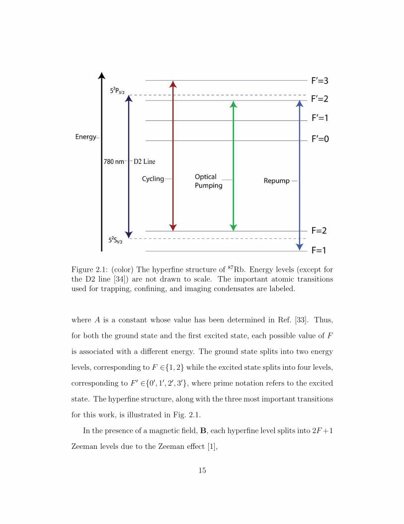
Figure 2.1: (color) The hyperfine structure of 87Rb. Energy levels (except forthe D2 line [34]) are not drawn to scale. The important atomic transitionsused for trapping, confining, and imaging condensates are labeled.

where A is a constant whose value has been determined in Ref. [33]. Thus,

for both the ground state and the first excited state, each possible value of F

is associated with a different energy. The ground state splits into two energy

levels, corresponding to F ∈1, 2 while the excited state splits into four levels,

corresponding to F ′ ∈0′, 1′, 2′, 3′, where prime notation refers to the excited

state. The hyperfine structure, along with the three most important transitions

for this work, is illustrated in Fig. 2.1.

In the presence of a magnetic field, B, each hyperfine level splits into 2F+1

Zeeman levels due to the Zeeman effect [1],

15

∆E = mFgFµBB (2.5)

where mF ∈−F,−F + 1, ..., 0, ..., F − 1, F is the quantum number that de-

termines the projection of the total atomic angular momentum F along the

magnetic field vector B, and gF is the Lande g-factor for 87Rb in its ground

state, this quantity is, in the case where we ignore the negligible proton g-

factor, given by [1]

gF =F 2 + F − 3

F 2 + F, (2.6)

and is therefore −1/2 for F = 1 and 1/2 for F = 2. Using Eqs. 2.6 and 2.5 we

see that, for atoms in the F = 1 manifold, states with negative mf values will

have their energies shifted higher in a magnetic field, whereas in the F = 2

manifold, states with positive mf values have their energies shifted higher.

The Zeeman sub-levels for the F = 1 and F = 2 manifolds are illustrated in

Fig. 2.2.

The red lines in Fig. 2.2 represent states in which the energy increases in

the presence of a magnetic field. If we were to create a local magnetic field

minimum at some point in space, atoms in these states would be attracted

to that point in order to minimize their potential energy. This is why atoms

in these states are typically described as ‘weak field seeking.’ We exploit this

property to create the magnetic trap (see section 2.2.2).

There are three important transitions, labeled in Fig. 2.1, between the

hyperfine levels that we use to confine, cool, and image atoms. The most

16

Figure 2.2: (color) Zeeman splitting of the ground state of 87Rb. Energy levelsare not drawn to scale. Red lines represent states that are weak field seeking,and can thus be attracted to a local field minimum.

17

important of these is labeled the ‘cycling’ transition, |2, 2〉 → |3′, 3′〉. We call

it the cycling transition because it can be driven repeatedly, which makes it

useful for the purposes of laser cooling (see section 2.2.1). We drive the cycling

transition by shining σ+ circularly polarized light, tuned to resonance with the

F = 2 to F ′ = 3′ transition, at atoms in the |2, 2〉 state. This brings the atoms

to the |3′, 3′〉 state, since mF must increase by 1 whenever an electron absorbs

σ+ polarized light in order to conserve angular momentum. The atoms then

decay from the |3′, 3′〉 state. Decays from a higher energy state to a lower one

are determined by the selection rules, ∆F = ±1, 0 and ∆m = ±1, 0. Thus, a

decay from the |3′, 3′〉 state to the ground state necessarily leaves the atom in

the |2, 2〉 state, where the cycling process can begin again. We use the cycling

transition for laser cooling (section 2.2.1) and imaging (section 2.2.4).

An atom may undergo an off-resonant (and ‘off-polarization’) transition to

the F ′ = 2′ manifold in the presence of light tuned to the cycling transition.

In this event, the atom decays with nonnegligible probability to the F = 1

manifold, where it is no longer resonant with the cycling transition. In order

to bring atoms in the F = 1 manifold back to the F = 2 manifold, we expose

the atom to light tuned to the ‘repump’ transition. The repump light transfers

atoms from the F = 1 manifold to the F ′ = 2′ manifold, from which the atom

may decay back into the F = 2 manifold, whence it is again subject to light

tuned to the cycling transition. If the atom instead decays back into the F = 1

manifold, we drive the ‘repump’ transition again to give us another chance to

bring it to the F = 2 manifold.

The last useful transition is the ‘optical pumping’ transition, between the

18

F = 2 and F ′ = 2′ manifolds. We drive this transition with σ+ circularly

polarized light in order to bring atoms in states where mF < 2 to the |2, 2〉 state

before loading them into the magnetic trap (Sec. 2.2.2). This works because,

when the atom absorbs the σ+ circularly polarized light, mF increases by one.

The atom then decays, at which point mF changes by ∆mF = ±1, 0. The

atom can then absorb more σ+ polarized light, until eventually it reaches the

|2, 2〉 state, at which point it cannot absorb any more σ+ light.

2.2 The BEC Refrigerator

In this section we consider the steps required to make and image a BEC. We

start by trapping the atoms in a Magneto-optical Trap (Section 2.2.1), which

increases the phase-space density to within five orders of magnitude of the

required density for Bose-condensation [35]. Then, we transfer the atoms into

a magnetic trap (Section 2.2.2). The magnetic trap allows us to further in-

crease the phase-space density before we begin the evaporative cooling process

(Section 2.2.3). Evaporative cooling removes the most energetic atoms, which

reduces the temperature of the condensate enough to reach the phase-space

density required for macroscopic population of the ground state. We then dis-

cuss how we take data by imaging the condensates (Section 2.2.4). The section

concludes with a discussion of extraction imaging, which we use to study the

real-time dynamics of a BEC (Section 2.2.5) [8, 9].

19

2.2.1 Magneto-Optical Trap

Magneto-optical traps (MOTs) utilize both magnetic fields and laser light to

trap atoms. Atoms are trapped when they are stably confined to a certain

volume.

The principles behind laser cooling are quite simple [1, 36–38]. We fo-

cus three orthogonal pairs of counter-propagating laser beams, which are all

slightly red-detuned (i.e. tuned to a lower frequency) from resonance with the

‘cycling’ transition (Fig. 2.1) on the atoms in the trap. Atoms moving towards

a laser see the red-detuned light from that laser blue-shifted (i.e. shifted to a

higher frequency) closer to resonance via the Doppler effect, and will absorb

a photon from that laser, bringing the atom to the |3′, 3′〉 state. The absorp-

tion of a photon reduces the component of the velocity of the atom opposite

that of the direction of laser propagation by v = h/(mλ). This slowing effect

gives this type of laser cooling its nickname, ‘optical molasses.’ The atom will

eventually decay back to the |2, 2〉 state, where it can continue to be slowed

down by further absorption of laser light.

Adding a magnetic field gradient provides a means of providing spatial

confinement in conjunction with the optical molasses. We generate the field

gradient by running current through a pair of anti-Helmholtz coils. We can

then use a system of coordinated beam polarization to take advantage of the

Zeeman shift resulting from the introduction of the magnetic field gradient in

a way that confines atoms to a region near the center of the trap. [1, 22, 31].

Our apparatus employs a double MOT system. Rubidium-87 atoms are

loaded into the first of our two MOTs, which we call the ‘collection MOT,’ by

20

heating a so-called ‘Rb getter.’ In order to further cool the atoms we must

isolate the 87Rb atoms from background atoms. We do this by transferring

them to the ‘science’ MOT, which is held under a higher vacuum than the

collection MOT. We transfer the atoms by sending brief pulses of laser light,

tuned to the cycling transition, from the collection MOT to the science MOT.

Photons are repeatedly absorbed by atoms, which provides net momentum

kicks in the direction of the science MOT.

Sadly, we can’t quite reach the phase-space density Dc required for con-

densation using only MOTs, since there is an upper limit on the phase-space

density for a cloud of atoms trapped in a MOT which is about 105 orders of

magnitude above Dc [35]. We must continue to reduce T and/or increase n.

To do this, we must transfer the atoms to a trap which uses only magnetic

fields for confinement.

In order to prepare the atoms to be magnetically trapped, we further red-

detune the MOT beams and reduce the magnetic field gradient. As a result,

atoms scatter less light, which reduces the scattered photon pressure within the

gas. This reduction in the scattered photon pressure causes a corresponding

reduction in the interatomic collision frequency, which increases the atomic

density. This is why we call this stage the compressed MOT stage (CMOT)

[39]. In addition to increasing the atomic density, the CMOT also heats the

gas, since the efficacy of laser cooling is reduced when the MOT beams are

detuned.

We then move to optical molasses by re-tuning the trapping beams closer

to resonance and reducing the magnetic fields, causing the cloud to expand

21

and cool. After a brief period of cooling we prepare the atoms for magnetic

trapping by using the optical pumping transition, in the presence of a rotating

bias field, to bring them to either the |1,−1〉 state or the |2, 2〉 state, both of

which can be magnetically trapped (Fig. 2.2) [29, 30].

2.2.2 Magnetic Trapping

To magnetically trap the atoms we use a pair of anti-Helmoltz coils to create

a magnetic field given by Eq. 2.7 [1, 27]

B = B′x x +B′y y − 2B′z z, (2.7)

where B′ is the magnetic field gradient along the x and y axes. Equation 2.7

indicates that the magnetic field vanishes at the origin. This minimum defines

the center of the trap. A point in space which is magnetic field minimum is

also an energy minimum (see Section 2.1) for the weak-field seeking states of

87Rb. Therefore, atoms in the 87Rb gas are attracted to the center of the trap

if they are in one of the three weak field seeking states. We typically use atoms

in the |1,−1〉 weak-field seeking state.

This magnetic trap rapidly loses atoms as they are cooled. These losses

occur when atoms move through the field minimum, undergoing transitions

to un-trapped (or anti-trapped) states within the same hyperfine manifold.

They then exit the trap. These transitions are called Majorana transitions,

and must be avoided if we are to cool the atoms to degeneracy. [40].

We circumvent this problem by using a time-averaged orbiting potential

22

(TOP) trap [41]. The TOP trap superposes a ‘rotating’ bias field on the static

field gradient produced by the anti-Helmholtz coils. This bias field may be

written [1, 27]

Bbias(t) = (B0 cosωt) x + (B0 sinωt) y, (2.8)

where B0 is the field magnitude and ω = (2π)×2 kHz is the angular frequency

at which the field vector rotates. Adding the bias field to the quadrupole field

(Eq. 2.7) yields

B(t) = (B′x+B0 cosωt) x + (B′y +B0 sinωt) y − 2B′z z. (2.9)

The addition of the rotating bias field displaces the minimum of the combined

magnetic field from the origin and causes the minimum to rotate in the hori-

zontal plane. For traps in which all of the atoms are located at a radius such

that r |B0/B′|, the magnitude of this field is given by [1]

B(t) =[(B0 cosωt+B′x)

2+ (B0 sinωt+B′y)

2+ 4B′2z2

]1/2

≈ B0 +B′ (x cosωt+ y sinωt) +B′2

2B0

[x2 + y2 + 4z2 − (x cosωt+ y sinωt)2]

(2.10)

We choose a bias field strong enough to displace magnetic field mini-

mum outside the cloud of atoms, thereby preventing Majorana transitions

(see Fig. 2.3). The atoms attempt to ‘chase’ the rotating minimum, but move

23

Figure 2.3: (color) An illustration of the TOP Trap. The location of themagnetic field zero rotates at ω/2π=2 kHz outside the cloud of atoms, therebypreventing Majorana transitions.

so slowly in comparison to the 2 kHz rotation that their displacement from the

center of the trap is negligible.

The potential energy of an atom in a state s as a function of its position

within the trap, according to Eq. 2.5, is

Es = Cs − µsB(t) (2.11)

where Cs is a constant and µs = mfgfµB is the magnetic moment associated

with the internal state of the atom. The relatively low speed of the atoms

compared to the rotation frequency of the trap allows us to consider only the

time averaged magnitude, 〈B〉t, when determining the potential energy of the

atoms in the magnetic trap. The time averaged magnitude for a field B(t)

given by Eq. 2.9 is

24

〈B〉t =ω

2π

∫ 2π/ω

0

B(t) dt ≈ B0 +B′2

4B0

(x2 + y2 + 8z2

). (2.12)

Using Eq. 2.12, we find that the potential of an atom in the magnetic trap is

Es = Es (B0)− µs (B0)B′2

4B0

(x2 + y2 + 8z2

). (2.13)

Therefore, we see that the combination of the oscillating bias field and the

quadrupole field results in an anisotropic harmonic potential:

V (x, y, z) =1

2ω2rr

2 +1

2λ2ω2

rz2, (2.14)

where ωr =√µsB′2/2mB0 and λ =

√8. For our trap, ωr/2π is found experi-

mentally to be 36.3 Hz.

2.2.3 Evaporative Cooling

Once the atoms are safely loaded into the TOP trap we can begin the final step

of the cooling process, evaporative cooling. During this process, we remove the

most energetic atoms in the cloud. This reduces the total energy per particle

of atoms within the cloud and, after rethermalization, the temperature of the

system.

We do this by taking advantage of the spatial dependence of the magnetic

field. The magnitude of the magnetic field, and thus the magnitude of the

Zeeman shift between trapped and untrapped states, increases with the dis-

tance from the center of the trap. We apply an RF field to the atoms that

drives transitions between trapped and untrapped states for the atoms with

25

the highest potential energy. The RF field removes all atoms past a certain

radius rRF, the radius from the trap center at which the RF field is resonant

with the frequency associated with the energy gap between Zeeman states,

from the trap. This process preferentially removes energetic atoms from the

trap, since atoms further from the center of the trap have a higher potential

energy. Removing these atoms is important because, when they move towards

the center of the trap, their potential energy is converted to kinetic energy,

which results in the heating of the condensate.

To continue removing the most energetic atoms from the condensate, we

further reduce rRF by lowering the frequency of the field. We do this slowly

enough for the atoms to continuously rethermalize after the energetic atoms

have been removed. This allows us to reduce the energy per particle of the

gas until the temperature has reached Tc, the critical condition for Bose-

condensation defined in Eq. 2.3. An illustration of this process is shown in

Fig. 2.4.

Once we have successfully produced a condensate, we maintain the RF

radiation to shield the cold sample from energetic atoms that have escaped

from the cooling process or that arise from inelastic heating. These ‘RF shields’

provide significantly longer condensate lifetimes.

2.2.4 Imaging

We collect experimental data by taking pictures of the condensates. This is

difficult to do in-situ since the radial extent of a BEC is on the order of 10µm,

and our imaging resolution is only about 5µm; even worse, the characteristic

26

Figure 2.4: (color) An illustration of RF Evaporation. The picture on theleft is at the start of the evaporation process, when the frequency of the RFradiation field is so high that no atoms wander to the space where the RFradiation is resonant with the |1,−1〉 → |2, 0〉 transition. The picture onthe right is at the end of the evaporation process (t = tf ), when enough highenergy atoms have been evaporated (and thus removed from the trap) throughthe process of reducing the RF frequency such that T < Tc.

27

size of the vortex core is only a few hundred nanometers! Fortunately, the

condensate can be expanded prior to imaging. We do this by releasing the

BEC from the trap, causing the interatomic interaction energy to be converted

to kinetic energy and expanding the cloud. We typically image the atoms with

laser beams that are directed either parallel to the axis of symmetry of the

condensate (generating a ‘top’ image of the condensate) or perpendicular to

that axis (generating a ‘side’ image of the condensate) after 23 ms of expansion.

The imaging process is illustrated in Fig. 2.5.

The absorptive imaging technique works as follows: First, after releasing

the atoms from the trap we shine laser light resonant with the cycling transition

at the atoms. The atoms absorb the light, and the beam is directed to a charge-

coupled device (CCD) camera, which records and rasterizes the beam profile.

The beam profile has a visible shadow where atoms scatter light from the laser

beam. Next, we take two more frames with the CCD camera, one in which

the probe beam is on (the ‘light’ frame) and one in which the probe beam is

off (the ‘dark’ frame). A computer then processes these images to determine

the atomic density of the BEC from the optical depth of the condensate. The

computer calculates the atomic density by subtracting the ‘dark’ frame from

the other two frames, and then calculating the light ratio of the ‘condensate’

frame to the ‘light’ frame for each pixel [42–44].

Since |1,−1〉 atoms do not respond to light at the cycling transitions, we

need to pump them into the F = 2 manifold. We do this by using microwave

radiation to transfer some percentage of atoms from the F = 1 to the F = 2

manifold as the atoms are falling and expanding after being released from the

28

To Top Camera

To Side Camera

low n high n

Top Camera

BEC

Side Camera

Figure 2.5: (color) Schematic of the imaging process. We direct a laser beam,tuned to resonance with the cycling transition, at the condensate. The atomsin the condensate absorb some of the photons in the beam. The beam is thendirected to either the side or the top camera. The data from the beam profileis sent to the computer, which computes the optical depth of the condensateand then converts the optical depth to atomic density. The computer thengenerates an image based on the calculation of the atomic density.

29

trap [8, 26]. Unsaturated images of |1,−1〉 condensates can be obtained by

imaging only a portion of the atoms in this way. [26].

2.2.5 Extraction Imaging

Recently we have developed a way to take pictures of the condensate in real

time [8, 9]. This allows us to study the real-time vortex dynamics of a BEC,

and has opened up many experimental possibilities. We briefly summarize this

process here; it is explained in greater detail in Ref. [8].

To image the condensate in real time, we extract portions of the condensate

by sending a short, spectrally broad microwave pulse tuned to resonance with

the transition from the |1,−1〉 state to the |2, 0〉 state. It is important that

the pulse be spectrally broad since the resonant frequency of the transition

differs depending on the position of the atom in the magnetic field (due to

the Zeeman shift). A spectrally broad pulse therefore allows us to extract

atoms from all sections of the condensate, providing a representative, and

presumably faithful, sample. The source of the microwave pulse is a 20 W

Hughes traveling wave amplifier. We can transfer 5% of the atoms to the |2, 0〉

state by presenting the BEC with a 2 µs pulse [8]. All ‘extraction’ images

presented in this thesis are taken using 5% extraction. Fig. 2.6 provides a

visual guide to the extraction imaging process.

Atoms in the |2, 0〉 state are untrapped, so they fall due to gravity. We

then image the atoms using the top camera in a way similar to the imaging

method we introduced in the last section. During extraction, the trap (and in

particular the magnetic field gradient) remains on, thus, the cycling transition

30

Figure 2.6: (color) An illustration of the extraction imaging process. Thecondensate (the red dot) experiences a short, spectrally broad microwave pulse(the green arrows from the microwave horn), causing a small percentage ofatoms (the black particles) to fall and expand in the magnetic field gradient(blue arrows). After the extracted atoms have fallen for 23 ms, we image themfrom either the side or the bottom. Image adapted from Refs. [8] and [9].

31

frequency is affected by the Zeeman shift. This means that we cannot use the

same laser frequency to image the extracted atoms, since that frequency is now

off resonance. The solution is not difficult: we use a different laser beam that

is tuned to the Zeeman shifted resonance frequency of the cycling transition.

Another adjustment we make to the usual imaging method arises from the

relatively short interval between images required to successfully study vortex

dynamics. The precession frequency of a single vortex about the center of a

condensate is, for our trap parameters, on the order of a few Hz [8, 9, 20].

To resolve this vortex motion, we require images that are spaced by tens

of milliseconds. To do this, we utilize the Fast Kinetics (FK) mode of the

camera. In FK mode we mask most of the camera’s CCD array, so that

no light can reach it. The mask prevents double exposure as the previously

exposed portions of the CCD array are shifted behind it. We use the mask

to store up to nine 102×1024 pixel images. We take images in FK mode

in the same fashion described earlier (see section 2.2.4), but we only expose

a 102×1024 section of the 1024×1024 pixel CCD array. After an image is

exposed, it is shifted behind the mask. This allows us to extract and image

eight times. The ninth image is reserved for the remnant condensate, which we

image by turning off the trap and dropping the condensate, as in section 2.2.4.

Only after all of the images have been exposed do we transfer the data to the

computer. We then take the ‘light’ and ‘dark’ frames in the same fashion.

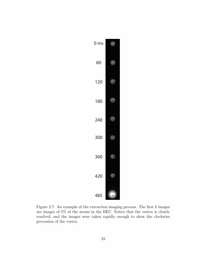
Fig. 2.7 shows an example of a set of extracted images.

32

0 ms

60

120

180

240

300

360

420

485

Figure 2.7: An example of the extraction imaging process. The first 8 imagesare images of 5% of the atoms in the BEC. Notice that the vortex is clearlyresolved, and the images were taken rapidly enough to show the clockwiseprecession of the vortex.

33

2.3 Deforming and Rotating the Magnetic Trap

The vortex generation experiments we discuss in Chapter 3 all rely on the

ability to deform and rotate the TOP trap (Sec. 2.2.2). Rotating the trap

means that the magnetic field minimum, instead of moving in a circle, moves

in the pattern of a rotating ellipse. This motion produces a time-dependent,

non-axisymmetric average trapping potential.

To rotate the trap we must:

• Elliptically deform the trap by applying a bias field where the x and y

components are unequal; and

• Modulate the components of the bias field such that the elliptically de-

formed trap rotates about the z-axis.

We perform both of these steps by modulating the current, at angular fre-

quency Ω, in the two pairs of coils that produce the bias field. This causes

the trap to become elliptically deformed and to rotate at angular frequency Ω.

These variations are illustrated in Fig. 2.8.

In the case where the trap is elliptically deformed but does not rotate, the

magnetic field produced by the bias coils is

Bbias(t) = (B0 +Bmod) cosωt x + (B0 −Bmod) sinωt y (2.15)

where Bmod is the magnitude of the additional field component produced by the

modulating current. Since the magnitude of the x component of the bias field

increases by roughly the same amount that the y component decreases, the

34

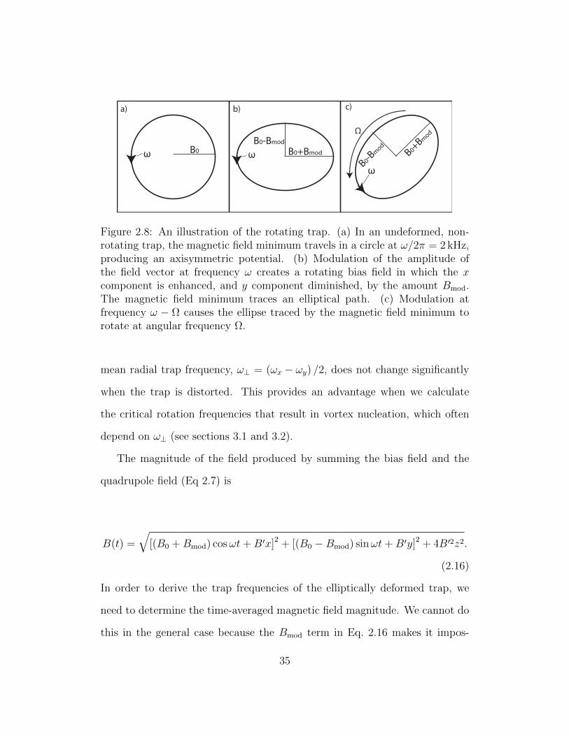
a) b) c)

Ω

ω

ω B0 ωB0-Bmod

B0+Bmod

B0-Bm

od B0+B

mod

Figure 2.8: An illustration of the rotating trap. (a) In an undeformed, non-rotating trap, the magnetic field minimum travels in a circle at ω/2π = 2 kHz,producing an axisymmetric potential. (b) Modulation of the amplitude ofthe field vector at frequency ω creates a rotating bias field in which the xcomponent is enhanced, and y component diminished, by the amount Bmod.The magnetic field minimum traces an elliptical path. (c) Modulation atfrequency ω − Ω causes the ellipse traced by the magnetic field minimum torotate at angular frequency Ω.

mean radial trap frequency, ω⊥ = (ωx − ωy) /2, does not change significantly

when the trap is distorted. This provides an advantage when we calculate

the critical rotation frequencies that result in vortex nucleation, which often

depend on ω⊥ (see sections 3.1 and 3.2).

The magnitude of the field produced by summing the bias field and the

quadrupole field (Eq 2.7) is

B(t) =

√[(B0 +Bmod) cosωt+B′x]2 + [(B0 −Bmod) sinωt+B′y]2 + 4B′2z2.

(2.16)

In order to derive the trap frequencies of the elliptically deformed trap, we

need to determine the time-averaged magnetic field magnitude. We cannot do

this in the general case because the Bmod term in Eq. 2.16 makes it impos-

35

sible to derive an analytical expression for the time-averaged magnetic field

magnitude in the same way in which we derived Eq. 2.12. In the limit that

the ratio between the magnitude of the bias field along the x and y axes,

C = (B0 +Bmod) / (B0 −Bmod), is small, however, the ratio between the x

and y trap frequencies is given by [12]

ωxωy

=1

4(C − 1) + 1. (2.17)

In the following chapters we will be concerned with the ellipticity of the trap-

ping potential,

ε =(ωy/ωx)

2 − 1

(ωy/ωx)2 + 1

= 1− 2

[(C/4) + (3/4)]2 + 1.(2.18)

In order to rotate the elliptical trap deformation at angular frequency Ω,

we make Bmod in Eq. 2.15 time dependent. We can determine the x and y

components of the bias field at a given time t by applying a rotation matrix to

the x and y components of the modulation term in the non-rotating elliptically

deformed bias field (Eq. 2.15)

Bx

By

=

B0

1 0

0 1

+Bmod

cos Ωt sin Ωt

sin Ωt − cos Ωt

cosωt

sinωt

, (2.19)

producing a trap with a magnetic field minimum that traces a rotating ellipse,

as in Fig. 2.8(c).

36

Chapter 3

Vortex Generation

There are many methods of generating vortex lines in Bose-Einstein conden-

sates (BECs), including rotating the trapping potential during evaporative

cooling (Sec. 2.2.3)[10, 13], exciting the dynamically unstable quadrupole mode

[11, 12, 14], shedding a vortex dipole in response to a moving barrier [16],

and spontaneous generation of vortex lines during rapid evaporative cooling

[8, 9, 15]. In this chapter we discuss two of these methods in depth: (1)

the generation of vortices by quenching from a thermal cloud to a condensate

while in a rotating potential (Section 3.1); and (2) the production of vortices

through an excitation of the quadrupole mode (Section 3.2.1). We also discuss

how we can combine these two processes to create vortex/antivortex clusters.

37

3.1 Vortex Generation by Evaporating in a

Rotating Frame

We can reliably create a condensate containing one or more vortices, all of

which are circulating in the same sense as the trap rotation, by rotating

and elliptically deforming the axisymmetric trap (see section 2.3) as we Bose-

condense the cloud of 87Rb atoms. This is similar to the experiment in Ref. [10],

which used a laser beam instead of a magnetic deformation to create the ro-

tating trap.

The effect of rotating the trap at some angular frequency Ω is to change

the energy of the condensate. In a frame rotating with the trap, the energy of

the condensate becomes

E ′ = E − L ·Ω, (3.1)

where E ′ is the energy of the condensate in the rotating frame, E is the energy

of the condensate in a non-rotating frame, L is the angular momentum, and

Ω is the angular velocity vector describing the rotation of the trap. When

L is zero (i.e., there are no vortex lines) the energy of the condensate is the

same in both reference frames. When L is non-zero, however, the energy of

the condensate is affected by the rotation of the trap. Figure 3.1 illustrates

how the energy of the condensate changes in a rotating frame.

A condensate with a vortex line becomes energetically favorable when Ev,

the energy of a condensate containing a vortex, is less than E0, the energy

of a vortex-free condensate. Assuming that L and Ω are parallel, Eq. 3.1

38

BEC BEC

BEC BEC

VortexCoreΩ

Ω

Non-Rotating Frame Rotating FrameN

o Vo

rtex

Vort

ex

E=E0 E=E0

E=EE=E - L Ω

v

v v

VortexCore

Figure 3.1: (color) Illustration showing how the energy of the condensatechanges in a rotating frame. The energy of the vortex state is indicated byEv while the angular momentum of the condensate is indicated by Lv. Con-densates with no vortices have no angular momentum (since condensates areirrotational, see Section 1.2), so the energy of a vortex-free condensate is un-affected by rotating the trap. However, condensates containing a vortex (andthus with non-zero angular momentum) have their energy reduced in a rotatingframe.

39

indicates that the critical rotation frequency, Ωc, at which the vortex state is

energetically favorable is given by

Ωc =EV 0 − E0

L, (3.2)

where EV 0 is the energy, in a non-rotating trap, of a condensate that contains

one vortex.

The difference in energies between a condensate with and without one

vortex, in the Thomas-Fermi approximation (which we discuss later in this

section) is given by [1]

EV 0 − E0 =4πn (0)

3

h2

mZ ln

(0.671

R

ξ0

), (3.3)

where n (0) is the density of the condensate at the center of the trap, m is the

mass of a 87Rb atom, R is the radial extent of the condensate, Z is the vertical

extent of the condensate, the 0.671 factor comes from a numerical integration

of the Gross-Pitaevskii equation in a rotating frame [1], and ξ0 is the healing

length, defined by

ξ0 =h√2mµ

. (3.4)

The angular momentum of a condensate in the Thomas-Fermi regime with

a vortex at its center is [1]

L =8π

15n (0)R2Zh. (3.5)

40

Using Eqs. 3.1, 3.5, and 3.3, we generate the expression for Ediff(Ω), the differ-

ence between Ev and E0 in a frame rotating at angular frequency Ω parallel

to L:

Ediff(Ω) =4πn (0)

3

h2

mZ ln

(0.671

R

ξ0

)− 8πΩ

15n (0)R2Zh. (3.6)

We also obtain an expression for Ωc by substituting Eqs. 3.3 and 3.5 into

Eq. 3.2, which yields

Ωc =5

2

h

mR2ln

(0.671

R

ξ0

). (3.7)

In order to calculate Ωc we need to be able to express R in terms of exper-

imental parameters and fundamental constants. We can do this fairly easily,

since our condensates are accurately described by the Thomas-Fermi approxi-

mation, valid when Na/a 1 [1]. For condensates produced in our apparatus,

Na/a > 1000, which easily satisfies this requirement.

In the Thomas-Fermi limit, the ratio of kinetic to potential energy is small

[1]. We therefore neglect the kinetic energy term in the Gross-Pitaevskii equa-

tion, yielding the algebraic equation

[V (r) + U0 |ψ (r)|2

]ψ (r) = µψ (r) (3.8)

which has the solution

n (r) = |ψ (r)|2 =[µ− V (r)]

U0

(3.9)

41

in the region where µ > V (r), and has the solution n (r) = 0 otherwise. The

condensate, therefore, extends to a radius r such that

V (r) = µ. (3.10)

For our trap, V (r) is given by:

V (x, y, z) =1

2m(ω2rr

2 + λ2ω2rz

2), (3.11)

where ωr is the radial trap frequency and λ = ωz/ωr, where ωz is the axial

trap frequency. If we substitute Eq. 3.11 into Eq. 3.10, we obtain

R2 =2µ

mω2r

. (3.12)

The chemical potential µ for a harmonically trapped condensate in the Thomas-

Fermi limit is [1]

µ =152/5

2

(Na

a

)2/5

hω, (3.13)

where N is the number of atoms in the condensate, a is the scattering length

for 87Rb, ω is the geometric mean of the trap frequencies, and a is the charac-

teristic length

a =

√h

mω. (3.14)

Substituting Eq. 3.13 into Eq 3.12, we obtain

42

R2 =152/5hω

mω2r

(Na

a

)2/5

. (3.15)

Finally, we can use Eq 3.15, Eq 3.14, and Eq 3.4 to rewrite the equation for

Ωc in terms of fundamental constants and experimental parameters:

Ωc =5ω2

r

2ω

(√h

mω

1

15Na

)2/5

ln

0.671ω

ωr

(15Na

√mω

h

)2/5 . (3.16)

For our trap, ωr/2π = 36.3 Hz, ω/2π = 50.8 Hz, a = 5.45×10−9 m, and the

initial condensate size is typically about 8×105 atoms. Inserting these values,

along with the fundamental constants, into Eq(3.16) yields Ωc/2π = 3.73 Hz.

Figure 3.2, which shows Ediff vs. Ω (Eq. 3.6) for these conditions, confirms

this value.

We have been able to generate a condensate containing a single vortex by

rotating the trap at Ω/2π = 5 Hz while condensing (Fig. 3.3). We have also

observed that, as we increase Ω further above Ωc, the condensate contains

more than one vortex line. This is a consequence of Eq. 3.1. In the non-

rotating frame, the energy of a condensate containing multiple vortex lines is

larger than the energy of a condensate containing a single vortex line. When

Ω becomes large enough, however, the L ·Ω term causes multiple vortex states

to be energetically favorable compared to both the single vortex state and the

zero vortex state. We indeed observe that as Ω/2π becomes larger, the number

of observed vortex lines increases.

For Ωc/2π between 28 Hz and 36 Hz, however, the condensate vanishes

43

Figure 3.2: (color) Plot of Ediff (Eq 3.6) for our trap parameters in the casewhere N = 8 × 105. We see that Ev becomes larger than E0 when Ω =23.44 rad/s = 2π · 3.73 Hz.

Figure 3.3: Images taken of a vortex state created by rotating the trappingpotential counter-clockwise at 5 Hz while evaporating a thermal cloud to acondensate

44

from the trap. We believe that this phenomenon is due to the ejection of

the condensate resulting from rotating the trap at a frequency too close to

the radial trap frequency, 2π×(36.3 Hz) [45]. At Ω/2π > 36.3 Hz, we observe

condensates, albeit with no vortices.

Figure 3.4 shows a plot of the number of vortex lines observed versus

Ω, while Fig. 3.5 shows images of condensates produced in rotating traps at

various Ω.

Figure 3.4: Graph of Vortex Number vs. Ω/2π for evaporation in a rotatingtrap with an elliptical distortion ε = 0.194.

45

0 ms

90

180

270

360

450

540

630

655 5 10 12.5 15 20 22.5 25 27.5 Ω/2π (Hz)

Figure 3.5: Images of condensates produced in a rotating trap for various Ω/2π.The elliptical distortion, ε, is 0.194, and the evaporation time is 3500 ms.

46

3.2 Vortex Generation Through Quadrupole

Mode Excitations: Theory

We can also generate vortices by driving the quadrupole mode, which is the

l = 2, m = ±2 collective mode excitation (Sec. 3.2.1). We drive this mode

by weakly distorting the trap and then rotating the distortion in the same

manner as we do when we generate vortices during evaporation (Sec. 3.1).

This time, however, we rotate the trap after we have already produced a

condensate, and the vortex lines arise from a completely different process.

Dynamical instabilities associated with the quadrupole mode allow for the

generation of a low density region on the outside of the condensate (called the

‘outer cloud’) [11, 12, 46, 47], where vortices are nucleated. These vortices

eventually penetrate into the bulk condensate (the ‘inner cloud’), possibly as

a result of collisions between condensate fragments in the outer cloud with

atoms in the inner cloud. [15].

3.2.1 The Quadrupole Mode [1]

Collective modes of BECs in a trap are periodic density oscillations that are

solutions of the hydrodynamic equations (derived in Appendix A):

∂n

∂t+∇ · (nv) = 0, (3.17)

and

47

m∂v

∂t= −∇

(µ+

1

2mv2

), (3.18)

where

µ = V + nU0 −h2

2m√n∇2√n (3.19)

and U0 = 4πh2a/m. We are interested in solutions of the form

n = n0 + δn, (3.20)

where n0 is the equilibrium density, and δn ∝ e−iωt. By considering the

velocity v, and the incremental density change δn to be small, we can rewrite

Eqs. 3.17 and 3.18 as

∂δn

∂t= −∇ · (n0v) , (3.21)

and

m∂v

∂t= −∇δµ, (3.22)

where δµ = U0 δn (we ignore the kinetic energy, ∇2√n, in the Thomas-Fermi

limit). By taking the time derivative of Eq. 3.21 and replacing ∂v/∂t with

Eq. 3.22, we obtain

m∂2δn

δt2= ∇ · (n0∇δµ) . (3.23)

48

Since we are interested in solutions where δn ∝ e−iωt, Eq. 3.23 can be rewritten,

by using the product rule of vector calculus, as

−ω2δn =U0

m

(∇n0 · ∇δn+ n0∇2δn

), (3.24)

where we have replaced δµ with U0 δn.

To find n0, we substitute Eq. 3.11 and Eq. 3.12 into Eq. 3.9, yielding

n0 =µ

U0

(1− r2

R2− λ2z2

R2

), (3.25)

where R is given by Eq. 3.12. Substituting Eq. 3.25 into Eq. 3.24 yields, after

some manipulation,

ω2δn = ω2r

(r∂

∂r+ λ2z

∂

∂z

)δn− ω2

r

2

(R2 − r2 − λ2z2

)∇2δn. (3.26)

Equation 3.26 can be solved analytically. The class of solutions which are

important for discussing the quadrupole mode are those where l = |m|. These

solutions are given by [1]

δn ∝ rlYl,±l (θ, φ) e−iωt. (3.27)

To get ω we substitute Eq. 3.27 into Eq. 3.26 which, since ∇2δn = 0, yields

ω2l = lω2

r , (3.28)

where ωl is the frequency of the density oscillation for a mode with total

49

angular momentum l.

To resonantly drive the quadrupole mode we do not rotate the trap at the

resonant frequency of the mode, ωl. This is because the centrifugal term in the

Hamiltonian (Eq. 3.1), −ΩLz, shifts the surface mode frequency by −lΩ [48].

Resonantly driving the quadrupole mode therefore requires that we rotate the

trap at a frequency Ω such that

2Ω = ωl =√

2ωr. (3.29)

Thus, Ωc = ωr/√

2.

3.2.2 Vortex Nucleation Process

Simply exciting the quadrupole mode does not generate vortex lines; we need

some mechanism for nucleating the vortices. If this weren’t the case, then

we would see vortices whenever the trap is rotated at Ω/2π > 3.73 Hz, since

that is the point at which a vortex state is energetically favorable according to

the results from Section 3.1, and we wouldn’t need to excite the quadrupole

mode at all to generate vortices in a Bose-condensed gas of atoms. Since

vortices have been observed after the quadrupole mode is excited [11, 12, 14],

the vortex generation mechanism is most likely associated with a quadrupole

mode excitation.

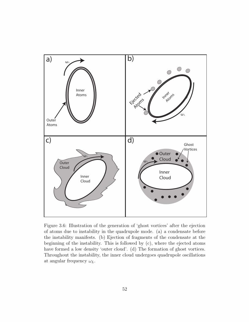
Vortices nucleated during a quadrupole mode excitation are believed to

result from a three step process, which we first briefly summarize; afterwards,

we provide a more detailed explanation [46]:

50

• For certain rotation frequencies and elliptical deformations, rotating the

trap creates a dynamical instability within the condensate, causing it

to eject material into an outer, low density, cloud where vortices are

nucleated [46, 48]. We call these vortices ‘ghost vortices’ because they are

invisible while in the low density outer cloud [49]. Figure 3.6 illustrates

this process.

• The elliptical condensate becomes more and more asymmetric due to

fluctuations in the two-fold symmetry (i.e. the condensate becomes less

symmetric across its long and short axis) of the condensate. When this

asymmetry becomes large enough, modes other than the quadrupole

mode can be excited, allowing for more energy and angular momentum

to couple into the system (in particular the outer cloud).

• The outer cloud recombines with the inner cloud. The energy and an-

gular momentum of the outer cloud is transferred to inner cloud, and

vortices are nucleated in the inner cloud, likely due to phase dislocations

in the merging condensate fragments, as in Ref. [15].

In previous experiments, vortices were observed after rotating the trap at

frequencies approximately resonant with the quadrupole mode driving fre-

quency [11, 12], indicating that the dynamical instability manifests when

the quadrupole mode is excited. To find out how these excitations of the

quadrupole mode can be dynamically unstable, we must first look at the so-

lutions to the Gross-Pitaevskii equation (GPE) in a frame rotating at angular

frequency Ω [47]

51

InnerCloud

Ejected

Atoms

InnerCloud

OuterCloud

Inner

Atoms

GhostVortices

OuterCloud

InnerAtoms

OuterAtoms

ω L

ω L

ω L

ω L

a) b)

c) d)

Figure 3.6: Illustration of the generation of ‘ghost vortices’ after the ejectionof atoms due to instability in the quadrupole mode. (a) a condensate beforethe instability manifests. (b) Ejection of fragments of the condensate at thebeginning of the instability. This is followed by (c), where the ejected atomshave formed a low density ‘outer cloud’. (d) The formation of ghost vortices.Throughout the instability, the inner cloud undergoes quadrupole oscillationsat angular frequency ωL.

52

ih∂ψ

∂t=

[− h2

2m∇2 + V (r, t) + U0 |ψ|2 − Ω(t)Lz

]ψ. (3.30)

The addition of the Ω(t)Lz term in the Hamiltonian forces us to add a rotating

term to the hydrodynamic equations, Eqs. 3.17 and 3.18, yielding

∂n

∂t+∇ · (nv)−∇ · n(Ω× r) = 0, (3.31)

and

m∂v

∂t= −∇

(V + nU0 −

h2∇2√n

2m√n

+1

2mv2 −mv · [Ω× r]

). (3.32)

Since we are in the Thomas-Fermi limit, we once again ignore the kinetic en-

ergy (∇2√n/√n) in Eq. 3.32. We now solve Eq. 3.32 for stationary solutions

(∂n/∂t = ∂v/∂t = 0) of n. We can assume that, since we are attempting to

drive the quadrupole mode, that the velocity field is an irrotational quadrupo-

lar flow of the form v = α∇ (xy). Using that assumption, we can solve for the

stationary solutions of n, which are [50]

n0 =1

U0

[µ− 1

2m(ωx

2x2 + ωy2y2 + ω2

zz2)], (3.33)

where

ωx2 =

[(1− ε) + α2 − 2αΩ

]ω2r , (3.34)

and

53

ωy2 =

[(1 + ε) + α2 + 2αΩ

]ω2r , (3.35)

in the region where µ > m(ωx2x2 + ωy

2y2 + ω2zz

2)/2; otherwise n0 = 0. The

modified trap frequencies ωx2 and ωy

2 can be thought of as the effective trap

frequencies induced by rotating the trap. Substituting Eq. 3.33 into Eq. 3.31

yields the solution [51],

α = −Ω

(ωx

2 − ωy2

ωx2 + ωy

2

). (3.36)

Just because a solution is a stationary solution of Eq. 3.36 doesn’t mean

that it is a stable solution, however. The stability of solutions to Eq. 3.36 can

be determined by considering small perturbations δn and δφ of the stationary

solutions for the density n0 and phase φ of the condensate [47, 50]. One can

do this by taking variational derivatives of Eq. 3.31 and Eq. 3.32 (since the

velocity is related to the phase by the relation v = h∇φ/m), which yields

[47, 50]

∂

∂t

δφδn

= −

(v −Ω× r) · ~∇ U0/m

~∇ · (n0~∇) (v −Ω× r) · ~∇

δφδn

(3.37)

Eigenfunctions of Eq. 3.37 vary in time with eλt, where λ is the eigenvalue

associated with the eigenfunction. The solutions to Eq. 3.37 are unstable

when one or more of the eigenfunctions blow up as time advances. Therefore,

if any eigenvalue of a solution to Eq. 3.37 has a positive real part, the solution

54

is unstable [47, 50].

Unstable combinations of ε and Ω have been determined by numerically

solving Eq. 3.37 [47, 50]. There are three ranges of instability associated

with the value of Ω/ωr. The instability that we most likely observe in our

experiments is the ‘ripple’ instability, as described in Ref. [50] and detailed in

the following paragraphs.

The ripple instability occurs when the trap is rotated at Ω/ωr < 1/√

2

and ε is linearly ramped past a critical value that depends on Ω. The start

of the instability is characterized by the ejection of atoms on the outside of

the condensate, eventually resulting in the formation of a low density ‘outer

cloud’, which does not undergo quadrupolar oscillations.

The numerical simulations also show that ‘ghost vortices’ form in the outer

cloud. This can possibly be explained by the process of phase negotiation

between the ’inner cloud’ (i.e., the atoms that have not been ejected from the

condensate) and the ‘condensate fragments’ in the outer cloud with which it

collides. As the inner cloud continues undergoing quadrupole oscillations, the

long axis of the inner cloud collides with atoms in the ejected outer cloud [46].

The order parameters of the inner cloud and the fragments in the outer cloud

have different phases. When they collide, a closed contour around the point of

collision between the inner cloud and the outer fragments occasionally encloses

a 2π phase winding. If so, when the inner cloud and the outer fragments come

into contact, a ‘ghost vortex’ can form in the outer cloud, since a 2*π phase

winding around a closed contour is a necessary condition for vortex generation

(Sec. 1.2). Then, when ε is increased past the critical value, the outer cloud

55

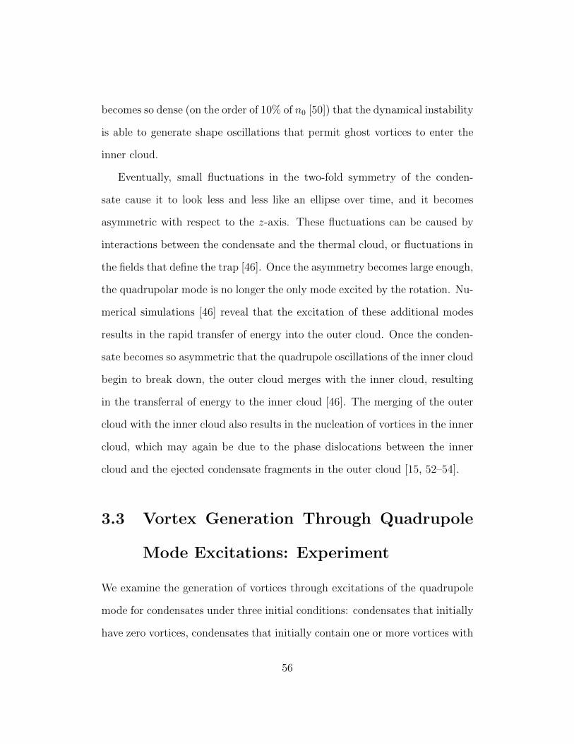
becomes so dense (on the order of 10% of n0 [50]) that the dynamical instability

is able to generate shape oscillations that permit ghost vortices to enter the

inner cloud.

Eventually, small fluctuations in the two-fold symmetry of the conden-

sate cause it to look less and less like an ellipse over time, and it becomes

asymmetric with respect to the z-axis. These fluctuations can be caused by

interactions between the condensate and the thermal cloud, or fluctuations in

the fields that define the trap [46]. Once the asymmetry becomes large enough,

the quadrupolar mode is no longer the only mode excited by the rotation. Nu-

merical simulations [46] reveal that the excitation of these additional modes

results in the rapid transfer of energy into the outer cloud. Once the conden-

sate becomes so asymmetric that the quadrupole oscillations of the inner cloud

begin to break down, the outer cloud merges with the inner cloud, resulting

in the transferral of energy to the inner cloud [46]. The merging of the outer

cloud with the inner cloud also results in the nucleation of vortices in the inner

cloud, which may again be due to the phase dislocations between the inner

cloud and the ejected condensate fragments in the outer cloud [15, 52–54].

3.3 Vortex Generation Through Quadrupole

Mode Excitations: Experiment

We examine the generation of vortices through excitations of the quadrupole

mode for condensates under three initial conditions: condensates that initially

have zero vortices, condensates that initially contain one or more vortices with

56

circulation in the same direction as the trap rotation, and condensates that

initially contain one or more vortices with circulation in the opposite direction

as the trap rotation. In the latter case, we observe counter-circulating vortices,

as one or more vortices circulating in a direction opposite that of the initial

vortex enter the condensate during the excitation.

In all cases we excite the quadrupole mode by fixing the stirring frequency

Ω, and linearly ramping on the deformation parameter, ε, from zero to εf =

0.0027 over 50 ms. Once the deformation parameter reaches εf we keep stirring

the trap for time tstir before ramping the deformation back down to zero over

50 ms.

3.3.1 Quadrupole Mode Excitations of Condensates with

Zero Vortices

In order to test how weakly rotating the trap affects a condensate contain-

ing zero vortices, we first generate a condensate and immediately image it

(Section 2.2.5) before we excite the quadrupole mode, in order to ensure the

condensate did not initially contain a vortex. This image is referred to as

the ‘before stirring’ image. We then rotate the trap at Ω for a time, tstir.

After rotating the trap, we take a series of images of the condensate in or-

der to determine the response of the condensate to the rotating trap. We

took two sets of images; one set with tstir = 1500 ms (Fig. 3.7), and the other

with tstir = 3000 ms (Fig. 3.8). Both sets of images show that the conden-

sate had the largest response to the rotation somewhere between Ω/ωr = 0.66

and Ω/ωr = 0.68, which is slightly below the resonant driving frequency for

57

the quadrupole mode excitation, Ω/ωr ≈ 0.707. Figure 3.9 shows a graph of

vortex number vs. Ω/ωr for condensates in which tstir = 3000 ms.

The fact that Ωc is below the quadrupole mode excitation frequency in-

dicates that the instability in this case is likely the ripple instability (Sec-

tion 3.2.2). We also note that we observe these instabilities for trap rota-

tions with ellipticity an order of magnitude lower than in previous experiments

[11, 12].

3.3.2 Quadrupole Mode Excitations of Condensates with

One or More Vortices

When there is a vortex present in the condensate, we observe the splitting

of the m = 2 and m = −2 quadrupole modes [55, 56]. This mode splitting

can be understood in comparison to the Sagnac effect, which was discovered

in Georges Sagnac’s experiments with rotating interferometers [57]. Sagnac

observed that the interference pattern produced by the two light sources in

the interferometer shifted while the interferometer was rotated: the rotation

causes one beam to traverse a longer distance than the other, since the position

of the detector has moved during the time the light takes to move from the

light source to the detector.

A similar effect is observed in a rotating condensate with one or more

vortex lines. Consider a condensate that contains one vortex line of counter-

clockwise circulation in its center. The atoms in the condensate all rotate

counter-clockwise about the center of the condensate. Now, if we rotate the

trap clockwise at a frequency Ω in the laboratory frame, we see that in a frame

58

beforestirring

0 ms

60

120

180

240

300

360

385 0.620 0.633 0.647 0.661 0.675 0.689 Ω/ω r

Figure 3.7: Images of initially vortex free condensates after weakly rotating thetrap CCW for tstir = 1500 ms. All condensates were stirred with a deformationparameter εf = 0.0027. One early picture was taken before stirring. Thestrongest reactions are at Ω/ωr = 0.661 and Ω/ωr = 0.675.

59

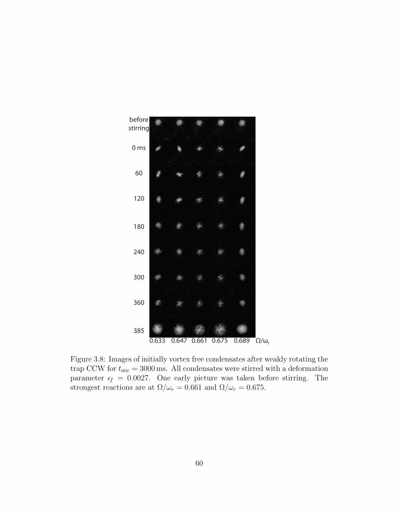
beforestirring

0 ms

60

120

180

240

300

360

3850.633 0.647 0.661 0.675 0.689 Ω/ω r

Figure 3.8: Images of initially vortex free condensates after weakly rotating thetrap CCW for tstir = 3000 ms. All condensates were stirred with a deformationparameter εf = 0.0027. One early picture was taken before stirring. Thestrongest reactions are at Ω/ωr = 0.661 and Ω/ωr = 0.675.

60

Figure 3.9: Graph of vortex number vs. Ω/ωr for condensates starting withzero vortices. All condensates were stirred with a deformation parameter, εf ,of 0.0027 for tstir = 3000 ms.

61

Figure 3.10: (color) An illustration of the Sagnac effect in a rotating conden-sate. In the lab frame, we see that the condensate ‘observes’ a trap rotationfrequency that differs from Ω. In the co-rotating case, this ‘observed’ rotationfrequency is Ω−ωcond, where ωcond is the rotation frequency of the condensate.In the counter-rotating case, the ‘observed’ rotation frequency is Ω + ωcond.This picture is a good approximation but is not entirely accurate, since therotation frequency of an atom in the condensate depends on how far that atomis from the condensate center.

rotating with an atom in the condensate the trap looks as if it is rotating at

a frequency greater than Ω. In this case, a mode excited by rotating the

trap at Ωc for a condensate with no vortices will now be excited by stirring

at a frequency slightly below Ωc, due to the increase in observed frequency.

Figure 3.10 shows an illustration of the Sagnac effect for a rotating condensate.

The magnitude of the mode splitting is [56]

62

ω+ − ω− =2〈lz〉M〈r2

⊥〉, (3.38)

where ω+ (ω−) is the quadrupole mode resonance frequency in the case of the

co-rotating (counter-rotating) trap, 〈lz〉 = h is the mean angular momentum

of the atoms in the condensate for condensates with one vortex in the center

(〈lz〉 < h if the vortex is not centered), and 〈r2⊥〉 = (2/7)R2 is the expectation

value of the square of the radial position of an atom in the condensate in the

Thomas-Fermi limit. Using Eq. 3.15 to substitute for R the mode splitting

becomes, for a single vortex in the center of the condensate,

ω+ − ω− =7ω2

r

ω

( a

15Na

)2/5

(3.39)

with a is given by Eq. 3.14. After stirring in a vortex by the method in

Section 3.1, our condensate typically has N ∼ 5.3×105 atoms. Substituting

into Eq. 3.39 yields (ω+ − ω−)/2π ≈ 2.94 Hz. According to Eq. 3.29, driving

the quadrupole mode on resonance requires stirring at Ω = ωl/2. There-

fore, the difference between the resonant driving frequency of the co-rotating

quadrupole mode, Ωco, and the resonant driving frequency of the counter-

rotating quadrupole mode, Ωcounter, should be

Ωco − Ωcounter

2π=ω+ − ω−2× (2π)

≈ 1.47 Hz. (3.40)

In order to test the validity of Eq. 3.40 we measured the response of a

one-vortex condensate to attempts at driving (εf = 0.0027) the m = +2 and

m = −2 quadrupole modes as a function of Ω. We generate condensates

63

with one counter-clockwise circulating vortex through the process described

in section 3.1. The response (determined by the number of additional vortices

generated after rotating the trap at Ω) in the co-rotating case is illustrated

in Fig. 3.11, while the response in the counter-rotating case is illustrated in

Fig. 3.12. Images of the condensates after exciting the co-rotating and counter-

rotating quadrupole resonances are shown in Figs. 3.13 and 3.14. Examining

Fig. 3.14 closely, it is clear that, in images where there are more than one

vortex (the middle three sets of images), the vortex closest to the center is

precessing counter-clockwise about the center, while all of the other vortices

are precessing clockwise, indicating that they have opposite circulations.

Based on the responses, displayed in Figs. 3.11 and 3.12, we determine that

Ωco/2π = 25.5 Hz and 23.5 Hz < Ωcounter/2π < 24 Hz. Therefore, 1.5 Hz <

(Ωco − Ωcounter) /2π < 2.0 Hz. This range excludes the 1.47 Hz predicted by

Eq. 3.40. The disparity may be explained by the fact that the vortices in our

condensates were not always centered, resulting in a lower 〈lz〉, and reducing

the value of the mode splitting predicted by Eq. 3.38

We have demonstrated that the frequencies of the two quadrupole modes

do indeed split in the presence of a vortex. Our ability to observe this splitting

by counting the additional vortices generated after stirring the trap at Ω helps

confirm that the quadrupole mode leads to the dynamical instability that

results in vortex nucleation [46, 47].

Equation 3.40 implies that as the angular momentum per atom increases,

the splitting between the quadrupole modes should also increase. Therefore,

if we start with more than one co-rotating vortex, we should observe a larger

64

Figure 3.11: Plot of the response (determined by number of additional vorticesgenerated after rotating the trap at Ω) of a one-vortex condensate to drivingthe quadrupole mode by rotating the trap in the same direction that the vortexcirculates vs. Ω/2π. The elliptical deformation of the trap was εf =0.0027,and tstir = 1500 ms. Based on the plot, we see that Ωco/2π is around 25.5 Hz.

65

Figure 3.12: Plot of the response (determined by number of additional vorticesgenerated after rotating the trap at Ω) of a one-vortex condensate to drivingthe quadrupole mode by rotating the trap in the direction opposite that inwhich the vortex circulates vs. Ω/2π. The elliptical deformation of the trapwas εf =0.0027, and tstir = 1000 ms. Based on the plot, we see that Ωcounter/2πis somewhere between 23.5 Hz and 24 Hz.

66

beforestirring

0 ms

60

120

180

240

300

360

385

24.5 25 25.5 26 26.5 Ω/2π (Hz)

Figure 3.13: Images of one-vortex condensates after driving the co-rotatingquadrupole mode. The first image is always taken before driving thequadrupole mode, and is used to verify that the condensate had a vortexbefore we excited the quadrupole mode. It is clear that the greatest responseoccurs at Ω/2π = 25.5 Hz.

67

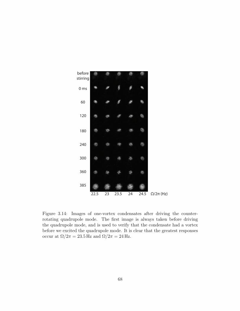
beforestirring

0 ms

60

120

180

240

300

360

385

22.5 23 23.5 24 24.5 Ω/2π (Hz)

Figure 3.14: Images of one-vortex condensates after driving the counter-rotating quadrupole mode. The first image is always taken before drivingthe quadrupole mode, and is used to verify that the condensate had a vortexbefore we excited the quadrupole mode. It is clear that the greatest responsesoccur at Ω/2π = 23.5 Hz and Ω/2π = 24 Hz.

68

splitting. To test this we perform the same experiment, but stir in two counter-

clockwise circulating vortices before exciting the quadrupole mode. Figure 3.15

indicates that Ωco/2π is around 25.5 Hz, as in the case with one vortex, while

Fig. 3.16 indicates that Ωcounter/2π is between 23 Hz and 23.5 Hz. Images of

the condensates after exciting the co-rotating and counter-rotating quadrupole

resonances are shown in Figs. 3.17 and 3.18. Figure 3.19 shows images of the

condensate after driving the co-rotating quadrupole mode for various tstir.

The responses, displayed in Fig. 3.15 and Fig. 3.16, indicate that Ωco/2π =

25.5 Hz and 23 Hz < Ωcounter/2π < 23.5 Hz in the case with two vortices. We

therefore have 2.0 Hz < (Ωco − Ωcounter) /2π < 2.5 Hz. We can see that the

upper and lower limits of the splitting have increased in the presence of an

additional vortex, as predicted.

3.4 Vortex Generation by Simultaneously Driv-

ing the m = 2 and m = −2 Quadrupole

Modes.

This section is devoted to the following questions: can we generate vortices

by driving both the m = 2 and m = −2 quadrupole modes at the same time?

Both modes can be driven at the same time by modulating the bias field in a

fashion similar to that used to rotate the trap (Sec. 2.3): we add an additional

sinusoidal term with frequency Ω2 to the modulation. To determine the x and

y components of the magnetic field at time t we apply a modified rotation

69

Figure 3.15: Plot of the response (determined by number of additional vorticesgenerated after rotating the trap at Ω) of a two-vortex condensate to drivingthe co-rotating quadrupole mode vs. Ω/2π. The elliptical deformation of thetrap was εf =0.0027, and tstir = 1500 ms. Based on the plot, we see thatΩco/2π is around 25.5 Hz.

70

Figure 3.16: Plot of response (determined by number of additional vorticesgenerated after rotating the trap at Ω) of a two-vortex condensate to drivingthe counter-rotating quadrupole mode vs. Ω/2π. The elliptical deformationof the trap was εf =0.0027, and tstir = 1000 ms. Based on the plot, we see thatΩcounter/2π is somewhere between 23 Hz and 23.5 Hz.

71

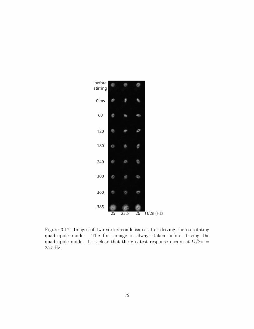
beforestirring

0 ms

60

120

180

240

300

360

385 25 25.5 26 Ω/2π (Hz)

Figure 3.17: Images of two-vortex condensates after driving the co-rotatingquadrupole mode. The first image is always taken before driving thequadrupole mode. It is clear that the greatest response occurs at Ω/2π =25.5 Hz.

72

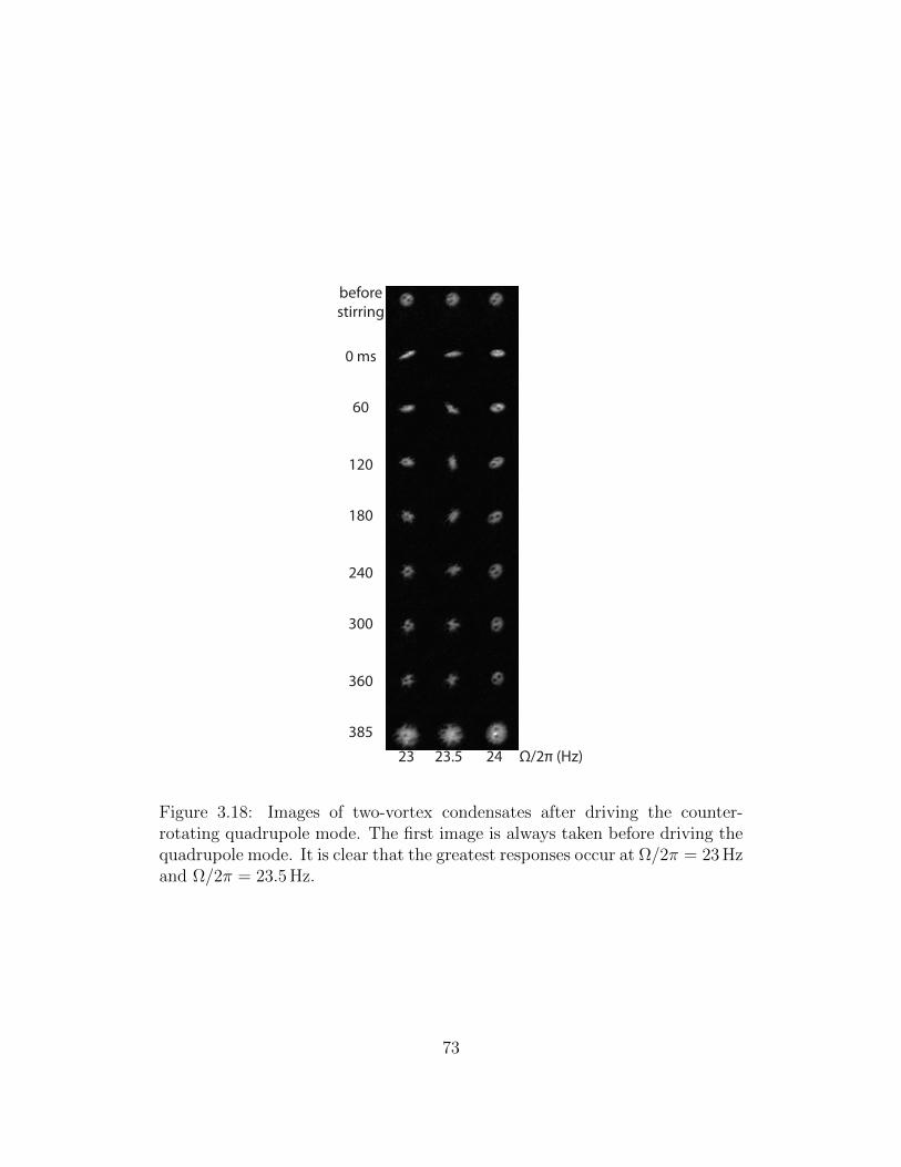
beforestirring

0 ms

60

120

180

240

300

360

385

23 23.5 24 Ω/2π (Hz)

Figure 3.18: Images of two-vortex condensates after driving the counter-rotating quadrupole mode. The first image is always taken before driving thequadrupole mode. It is clear that the greatest responses occur at Ω/2π = 23 Hzand Ω/2π = 23.5 Hz.

73

Figure 3.19: Images of two-vortex condensates after driving the co-rotatingquadrupole mode (at Ω/2π = 25.5 Hz) for various tstir.

74

matrix to the elliptically deformed field (Eq. 2.15):

Bx

By

=

B0

1 0

0 1

+Bmod1

cos Ω1t sin Ω1t

sin Ω1t − cos Ω1t

+Bmod2

cos Ω2t sin Ω2t

sin Ω2t − cos Ω2t

cosωt

sinωt

, (3.41)

where B0 is again the magnitude of the bias field, and Bmod1 and Bmod2 are

the amplitudes of the additional field components produced by the modulating

current. The magnitude of the x and y components of the bias field at time t

are then given by

Bx = B0 cosωt+Bmod1 cos (ω − Ω1) t+Bmod2 cos (ω − Ω2) t, (3.42)

and

By = B0 sinωt−Bmod1 sin (ω − Ω1) t−Bmod2 sin (ω − Ω2) t, (3.43)

respectively.

Although we do have the freedom to choose these parameters indepen-

dently, in the experiments described below we always set Ω2 = −Ω1 and

Bmod1 = Bmod2. Doing so causes the magnetic field minimum to follow the

path illustrated in Fig 3.20. Due to the periodic extensions of the trap along

the x and y axes which occur at angular frequency Ω = Ω1, we call this pro-

cess ‘stretching’ the trap. We define the ellipticity ε of the stretched trap to

75

be the same as the ellipticity of a rotating trap (see section 2.3) with a ratio

C = (B0 + 2Bmod) / (B0 − 2Bmod) between the magnitudes of the magnetic

field along the long and short axes.

We found that the response of the condensate to stretching the trap with

an ellipticity ε = 0.0054 for time tstretch depends on how many vortices the

condensate had before we stretched the trap. If the condensate contained

zero vortices before we stretched the trap at Ω/ωr = 0.675 (the value of Ω

resulting in the largest condensate response) for tstretch = 3.0 s we observed

that, though the condensate would become distorted after stretching the trap,

no additional vortices were nucleated (Fig. 3.21). We also tried stretching

the trap at different values in the ranges 0.0054 < ε < 0.126 and 24.5 Hz<

Ω/2π < 28 Hz. We have not yet found a combination of ε and Ω that results

in the generation of vortices, implying that driving the degenerate m = 2 and

m = −2 quadrupole modes at the same time does not produce the dynamical

instabilities required for vortex nucleation (section 3.2.2). This makes sense

because resonantly driving the m = 2 and m = −2 modes should have the

same effect as resonantly driving the sum of those two modes, which has m = 0.

The m = 0 mode is not known to produce vortices, so it is not surprising that

no vortices are generated by a process which, in effect, drives that mode.

In order to test the case where there is already a vortex in the condensate

we first stir in a counter-clockwise (CCW) circulating vortex by the method

in section 3.1. We then stretch the trap, with an elliptical distortion ε, at

angular frequency Ω for time tstretch. In this case, we were able to gener-

ate additional vortices that could be either co-circulating (CCW) or counter-

76

B0

B0

B0+Bmod

ωω

ω ω

a) b)

c) d)

t=0 t=π/2Ω

t=π/Ω t=3π/2Ω

B0-Bmod

B0+Bmod

B0-Bmod

Figure 3.20: Illustration of how we ‘stretch’ the trap at angular frequencyΩ = Ω1 = −Ω2 in order to excite both the m = 2 and m = −2 quadrupolemodes. (a) At t = 0 the trap is circular. (b) At t = T/4 (where T is theperiod), the trap is stretched along the y axis. (c) At t = T/2 the trap regainsits circular shape (d) At t = T/4 the trap is stretched along the x axis.

77

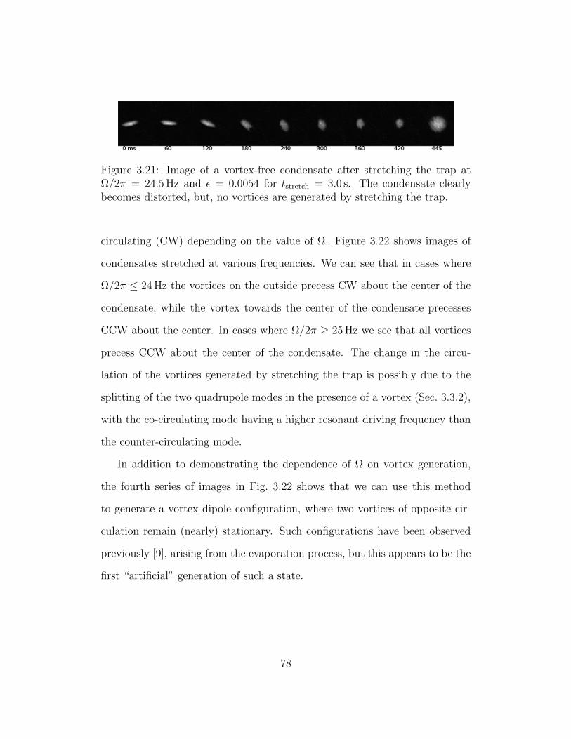
Figure 3.21: Image of a vortex-free condensate after stretching the trap atΩ/2π = 24.5 Hz and ε = 0.0054 for tstretch = 3.0 s. The condensate clearlybecomes distorted, but, no vortices are generated by stretching the trap.

circulating (CW) depending on the value of Ω. Figure 3.22 shows images of

condensates stretched at various frequencies. We can see that in cases where

Ω/2π ≤ 24 Hz the vortices on the outside precess CW about the center of the

condensate, while the vortex towards the center of the condensate precesses

CCW about the center. In cases where Ω/2π ≥ 25 Hz we see that all vortices

precess CCW about the center of the condensate. The change in the circu-

lation of the vortices generated by stretching the trap is possibly due to the

splitting of the two quadrupole modes in the presence of a vortex (Sec. 3.3.2),

with the co-circulating mode having a higher resonant driving frequency than

the counter-circulating mode.

In addition to demonstrating the dependence of Ω on vortex generation,

the fourth series of images in Fig. 3.22 shows that we can use this method

to generate a vortex dipole configuration, where two vortices of opposite cir-

culation remain (nearly) stationary. Such configurations have been observed

previously [9], arising from the evaporation process, but this appears to be the

first “artificial” generation of such a state.

78

beforestirring

0 ms

60

120

180

240

300

360

385

(23,2.5) (23,3.0) (24,4.0) (24,6.0) (25, 2.5) (25.5,2.0) (Ω/2π (Hz), t(s) )

0.0054 0.0054 0.0054 0.0054 0.0037 0.0054 ε

Figure 3.22: Images of one-vortex condensates after stretching the trap atvarious Ω. One image was taken before stretching the trap in order to confirmthat the condensate had a vortex before we stretched it. In cases where Ω/2π ≤24 Hz, the vortices generated on the outside of the condensate circulate in thedirection opposite that of the initial vortex. In cases where Ω/2π ≥ 25 Hz, allvortices circulate in the same direction.

79

Chapter 4

Vortex Manipulation

It can be useful to control the radial positions of the vortex lines in a Bose-

Einstein condensate (BEC). For example, we observe that the vortices gener-

ated by driving the quadrupole mode (Sec. 3.3) tend to be located in the outer

reaches of the condensate. We wish to study the behavior of vortices located

at different radial position in order to observe a diverse range of dynamics. In

this Chapter we discuss how to radially translate vortices by using frictional

interactions between the vortex cores and the surrounding atomic thermal

cloud. These are the first experiments, to our knowledge, that examine the

interaction between vortex lines and thermal clouds.

We begin by first introducing the theory of interactions between a vortex

core and a rotating thermal cloud, which indicates that the vortex core moves

towards (away from) the center of the condensate when the thermal cloud

rotates in the same (opposite) direction that the vortex circulates (Section 4.1).

We then present experimental observations of the radial translation of a vortex

80

caused by rotating the thermal cloud (Section 4.2). This chapter concludes

with our observations on the effect of rotating the thermal cloud surrounding

a condensate with more than one vortex line (Section 4.3).

4.1 Radially Translating a Single Vortex: The-

ory

To determine the effect of frictional interactions between a thermal cloud and

a vortex, we derive an analytical formula for the vortex motion of the form:

ds

dt=

(ds

dt

)0

+

(ds

dt

)f

(4.1)

where s is a three-dimensional curve describing the vortex line, and the 0 and

f subscripts indicate the motion of the vortex line in the absence and presence

of frictional effects, respectively. Since vortices in an oblate condensate are

parallel to the z-axis, we can take s to be the position of the vortex core.

Vortex motion without friction can be described by [58, 59]

(ds

dt

)0

= vs + vi. (4.2)

The self-induced velocity of the vortex line segment, vi, arises from Magnus

forces that involve the inhomogeneity of the condensate (see Sec. 1.2), or the

interaction of each line segment with the remainder of the line. The local

superfluid velocity at the core of the vortex, vs, arises from bulk motion of the

condensate. If there is more than one vortex, we must take into account the

81

velocity fields of the other vortices when determining vi.

The motion of a vortex that arises as a result of frictional effects has been

discussed in Ref. [59], and we follow that derivation here. When there is a net

relative velocity between the thermal cloud and the condensate, a frictional

force f will be exerted on the fluid surrounding the vortex core. Schwarz uses

momentum-conservation arguments to claim that this force f generates an

additional motion of the vortex described by [59]

(ds

dt

)f

=s′ × f

ρsκ(4.3)

where s′ is the unit tangent along the vortex, ρs is the superfluid density, and κ

is the quantized vorticity (κ = 1 for the vortices in a Bose-Einstein condensate;

see Sec. 1.2). The frictional force f has been experimentally determined to be

[59]

f

κρs= α

(vn −

(ds

dt

)0

)− α′s′ ×

(vn −

(ds

dt 0

)), (4.4)

where vn is the velocity of the thermal cloud, and α and α′ are parameters

that depend on the temperature. Substituting Eq. 4.4 into Eq. 4.3 yields

(ds

dt

)f

= αs′ ×(

vn −(ds

dt

)0

)− α′s′ ×

[s′ ×

(vn −

(ds

dt

)0

)]. (4.5)

Next we obtain an equation for the vortex motion by substituting Eq. 4.5

and Eq. 4.2 into Eq. 4.1, which yields

82

ds

dt= vi + vs + αs′ × (vn − vi − vs)− α′s′ × [s′ × (vn − vi − vs)] . (4.6)

The first two terms of Eq. 4.6 indicate that the motion of the vortex at T = 0,

where α and α′ are both zero, is described by vi (since vs = 0). The second

two terms indicate that, at T > 0, the thermal cloud exerts a force on the

vortex with strength determined by the temperature-dependent parameters α

and α′.

Let us now consider the solution of Eq. 4.6 when the thermal cloud and

condensate are both stationary (vs = vn = 0). Assuming that the vortex

lines are parallel to the axis of rotation, we see that the self-induced velocity

vi results only from the Magnus forces resulting from the inhomogeneity of

the condensate. This force causes the vortex to precess about the center of

the condensate in the direction of its circulation (Sec. 1.2)) [9, 20, 60]. In

cylindrical polar coordinates, vi = viφ and s′ = z. Substituting into Eq. 4.6

yields:

ds

dt= (vi − α′vi) φ+ αviρ. (4.7)

The azimuthal component of Eq. 4.7 is

(ds

dt

)φ

= vφ = vi − α′vi. (4.8)

Making the substitution vφ/rv = ωv, where rv is the radial position of the

vortex and ωv is the angular frequency at which the vortex precesses about

83

the center of the condensate, we obtain

ωv = (1− α′) virv. (4.9)

The radial component of the vortex motion is given by the second term in

Eq. 4.7,

(ds

dt

)r

= αvi. (4.10)

The temperature-dependent parameter α′ in Eq. 4.9 is typically very small

and can be ignored, allowing us to substitute Eq. 4.9 into Eq. 4.10 [58]. The

result is

ds

dt r=drvdt

= αωvrv, (4.11)

with solution

rv = r0eαωvt. (4.12)

Eq. 4.12 indicates that the radial position of the vortex core increases expo-

nentially until the vortex eventually leaves the condensate, provided we do not

rotate the thermal cloud (vs = vn = 0). Figure 4.1 demonstrates the increase

in rv as a function of time at various temperatures (parameterized by α).

Now let us consider the case where the thermal cloud is rotating about the

z-axis,

84

a) b)

c) d)

Figure 4.1: (color) The evolution of rv over time t as a function of α. (a)α = 0.0035, t = 26.0 s. (b) α = 0.02, t = 4.5 s. (c) α = 0.05, t = 1.85 s. (d) Aplot of the radius of the vortex versus time. In all cases the vortex is startingat (0.1, 0.0). This figure is adapted from Ref. [58]

85

vn = rvΩth, (4.13)

where Ωth is the angular frequency at which the thermal cloud rotates, taking

it to be positive if it is the same sense as ωv. Substituting Eq. 4.13 into Eq. 4.6

yields

ds

dt= [vi + α′ (rvΩth − vi)] φ+ [α (vi − rvΩth)] ρ, (4.14)

with azimuthal component

ωv =vi − α′ (rvΩth − vi)

rv= (1− α′) vi

rv− α′Ωth, (4.15)

and radial component

drvdt

= α (vi − rvΩth) . (4.16)

As before, we ignore α′ as a small quantity. Substituting Eq. 4.15 into Eq. 4.16

yields

drvdt

= α (ωv − Ωth) rv, (4.17)

which has solution

rv = r0eα(ωv−Ωth)t. (4.18)

According to Eq. 4.18, rotating the thermal cloud modifies the term in the

86

exponential that describes the time evolution of vr. This gives us a parameter

that we can adjust in order to cause the vortex to spiral outwards (Ωth < ωv)

or inwards (Ωth > ωv). For condensates in our trap, ωv ∼ 4 Hz.

We can understand this process through comparison with the numerical

simulations performed in Ref. [61], which demonstrate how the angular mo-

mentum per particle, l, of a condensate at T = 0 in a rotating trap increases

from 0 to h as a function of rv. First, a vortex approaches from the periphery

of the cloud when 0 < l < h. This displaces the center of mass of the con-

densate, causing it to rotate about the trap center. The orbit of the center of

mass then contributes additional angular momentum to the system. As the

angular momentum increases, the vortex core moves inward until it reaches the

center of the condensate, at which point l = h. At this point, in the absence

of a dynamical instability supporting the formation of additional vortices (see

Sec. 3.2.2), the condensate cannot gain any more angular momentum regard-

less of whether or not the condensate and the thermal cloud are in rotational

equilibrium.

In the case of T > 0, collisions between a thermal cloud rotating in the

same direction as the sense of velocity flow in the condensate should transfer

angular momentum to the condensate. This transfer of angular momentum

causes the vortex core to move inwards, since the angular momentum of a con-

densate containing a single vortex is maximized when the vortex core is at the

center. Likewise, collisions between a condensate and a thermal cloud rotating

oppositely should diminish the angular momentum per particle, causing the

vortex to move to larger rv. This process is illustrated in Fig. 4.2.

87

BEC

vortex

Thermal Cloud

ωv

ωv

ωv

ωv

L=L1

L=L1

L>L1

L<L1

Stationary RotatingΩ

> ω

vΩ

< ω

v

Ω

Ω

a)

c) d)

b)

Figure 4.2: (color) Illustration of the response of a condensate containinga vortex to a change in angular momentum caused by interactions with arotating thermal cloud. (a,c) A condensate with L = L1 with a vortex at r0

precesses about the center of the condensate. (b,d) If we rotate the thermalcloud, angular momentum is transferred from the rotating thermal atoms tothe condensate. (b) If the thermal cloud rotates in the same direction asωv, the angular momentum of the condensate increases, and the vortex movesinwards (blue arrow). (d) If the cloud rotates in the opposite direction, angularmomentum leaves the condensate and the vortex moves outward (blue arrow).

88

4.2 Radially Translating One Vortex: Experi-

ment

We now test the prediction that rotating the thermal cloud at Ωth > ωv in

the same direction that the vortex circulates pushes the vortex towards the

center. First, we generate condensates containing one vortex using the method

described in section 3.1. Next, we take a preliminary image of the condensate

(as in Section 2.2.5) in order to measure the initial radial position of the vortex.

We then permit a relatively large thermal cloud to form by increasing the

frequency of the radiofrequency shields (Section 2.2.3), effectively diminishing

its ability to remove atoms heated by inelastic collisions. We then rotate

the trap (Section 2.3) at angular frequency Ω and ellipticity ε for some time

tstir, forcing the entrained thermal cloud into rotation about the condensate.

After this rotation, we set ε = 0 and restore the shield frequency to bring

the temperature of the sample back down. Finally, we take a series of images

of the condensate. By comparing the radial position of the vortex in these

images to the radial position of the vortex in the first image, we can determine

whether the rotating thermal cloud has forced the vortex towards the center

of the condensate.

We do indeed observe that rotating the thermal cloud at Ω > ωv for a long

(10.8 full precessions of the vortex) period of time does force a vortex to move

towards the center of the condensate. Figure 4.3 shows a series of images of

a condensate stirred at Ω/2π = 16 Hz and ε = 0.102 for 43.2 full rotations of

the thermal cloud (tstir = 2.7 s) when the RF Shields were set to 4.85 MHz (as

89

opposed to 4.55 MHz that we usually set for a trap with ε = 0.102).

It is difficult to study the efficacy of this method when the initial radial

position of the vortex is different in each experimental run. We can circumvent

this difficulty by following the steps below (ε = 0.102 in all cases where we

rotate the trap in the steps below):

1. ‘Stir in’ the vortex : Determine a combination of tcenter and Ωcenter that

will force a vortex starting at any r0 to a radial position near the center

of the condensate. We then start with a condensate that has a vortex

near the center.

2. ‘Stir out’ the vortex : If we rotate the thermal cloud in the direction

opposite to the direction in which the vortex circulates, we can quickly

increase the radial position of the vortex. This allows us to choose a

particular rv as a starting point for studying the dependence of rv on t+stir

for fixed Ω+stir. In particular, for repeated trials conducted on condensates

starting with a vortex in the center, if Ω+stir and t+stir are fixed, the vortex

should always appear at the same radial position.

3. ‘Stir in’ the vortex (again): Then, since we can use steps 1 and 2 to

position a vortex at a fixed initial radius, we are able to study the de-

pendence of rv on t−stir for fixed Ω−stir by re-rotating the thermal cloud in

the same direction in which the vortex circulates.

90

beforestirring

0 ms

60

120

180

240

300

360

385

Figure 4.3: Images of a condensate containing one vortex after rotating thethermal cloud in the same direction as the vortex circulation. The first pictureverifies the existence of a single vortex prior to the rotation. The trap wasrotated at Ω/2π = 16 Hz for tstir = 2.7 s.

91

4.2.1 Stirring a Vortex to the Center

To determine the time, tcenter, required to stir a vortex at any initial r0 to

a region near the center of the condensate, we measure the radial position

of the vortex core after stirring at frequency Ωstir for a variable time tcenter.

The condensates initially contain one counter-clockwise circulating vortex line,

created by the method outlined in Sec. 3.1. An initial image of the condensate

(Section 2.2.5), verifies that it contains a solitary vortex. After the stirring is

complete, we take a set of images of the condensate.

If, in the first image, the vortex was near the periphery of the condensate,

and in the next images it is located near the center, then we conclude that

the chosen value of tstir is likely to push a vortex at any radial position to a

region near the center, and thus choose it to be tcenter. Figure 4.3 provides an

example: in the image taken before rotating the trap, the vortex is located

near the edge of the condensate. In subsequent images the vortex has been

translated to the center of the condensate. The parameters adopted in this

sequence are Ωcenter/2π = 16 Hz and tcenter = 2.7 s.

4.2.2 Stirring Out a Vortex

Using the method in section 4.2.1 allows for the generation of a condensate with

a vortex near its center. Fixing r0 in this way allows us to qualitatively observe

the dependence of rv on t+stir for a fixed Ω+stir. Figure 4.4 shows images of con-

densates that illustrate this dependence in the case where Ω+stir/2π = −15 Hz

(negative frequencies indicate a rotation of the trap in the opposite direction

to the vortex circulation; See Section 4.1). Figure 4.5 plots the radial position

92

of the vortex as determined from the final image of the condensate vs. t+stir.

We determine the radial position of the vortex by first fitting the condensate

and vortex to a truncated, inverted parabola and an inverted gaussian, respec-

tively. The radius of the vortex is then obtained by comparing the coordinates

of center of the gaussian to the center of the parabola [8].

We see from Fig. 4.5 that the results of this stirring do not obviously

describe an exponential growth in rv. One explanation is that small changes

in r0 drastically change the expected value of rv(t) expected for given values

of α and t+stir. From Eq. 4.18, we see that δrvr, the uncertainty in rv due to

uncertainty in r0 is

δrvr(t)

rv(t)=δr0

r0

. (4.19)

We found that the mean value for condensates that we declared to be ‘near’

the center of the condensate was r0/R = 0.1 and that the average uncertainty

in r0/R was 0.03. Substituting those values into Eq. 4.19 reveals that there is

a relative uncertainty of 30% in the expected value of rv due to the uncertainty

in r0.

We need to determine α in order to plot the expected exponential growth

curve for rv as a function of t+stir. To do so, we rearrange Eq. 4.18 to yield

ln rv(ωv − Ωth)

= αt+ln r0

(ωv − Ωth). (4.20)

Therefore, α is the slope of a graph of ln rv/ (ωv − Ωth) vs. t. Using the data

from the first five images in Fig. 4.4 we plot ln rv/(ωv − Ω+

stir

)vs. t+stir and

93

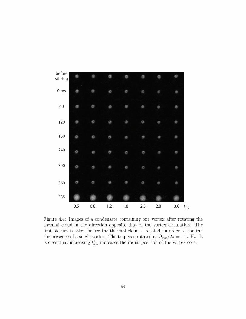
beforestirring

0 ms

60

120

180

240

300

360

385

0.5 0.8 1.2 1.8 2.5 2.8 3.0 t+stir

Figure 4.4: Images of a condensate containing one vortex after rotating thethermal cloud in the direction opposite that of the vortex circulation. Thefirst picture is taken before the thermal cloud is rotated, in order to confirmthe presence of a single vortex. The trap was rotated at Ωstir/2π = −15 Hz. Itis clear that increasing t+stir increases the radial position of the vortex core.

94

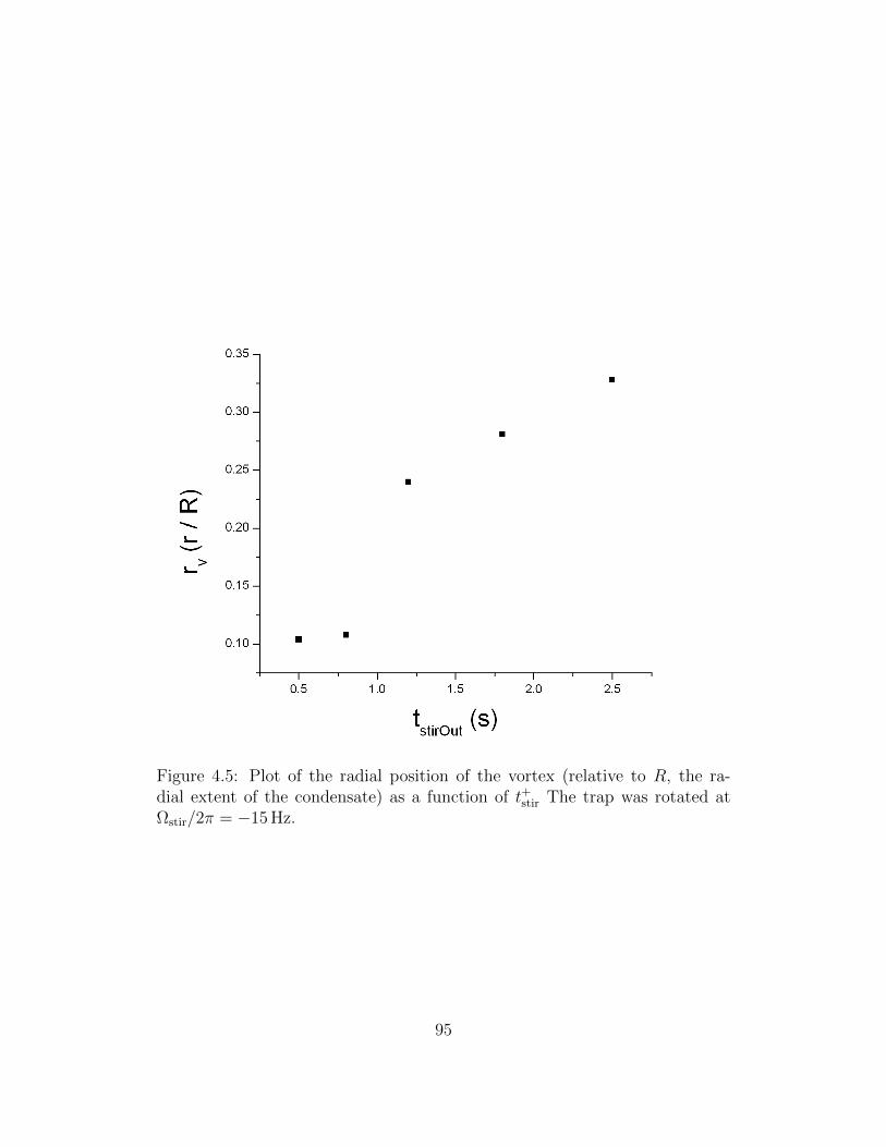
Figure 4.5: Plot of the radial position of the vortex (relative to R, the ra-dial extent of the condensate) as a function of t+stir The trap was rotated atΩstir/2π = −15 Hz.

95

Figure 4.6: (color) Plot of ln rv/(ωv − Ω+

stir

)vs. t+stir for the first five pictures

in Fig. 4.4. The red line is a linear fit to the data with slope α.

perform a linear regression to find α. The plot is shown in Fig. 4.6 and the fit

yields α = 0.0035± 0.0011. Inserting this result into Eq. 4.12, we predict that

a vortex starting at r0 will exit the condensate in 26(8) s if we do not rotate

the thermal cloud at all. This prediction is difficult to test directly, since the

decay time is considerably longer than a typical condensate lifetime.

In order to test the consistency of the data with the response predicted by

Eq. 4.18, we plot it on the same graph as rv(t). We also include an upper and

lower bound on the predicted rv based on the experimental uncertainty δrv.

96

In calculating δrv we must consider δrvα(t), the uncertainty in rv(t) caused

by uncertainty in α. From Eq. 4.18 we see that

δrvα(t) = [(ωv − Ωth) tthrv(t)] δα. (4.21)

Then, to find δrv(t) we sum Eq. 4.19 and Eq. 4.21 in quadrature, yielding

δrv(t) = rv(t)

√δr2

0

r20

+ (ωv − Ωth)2 t2δα2. (4.22)

The resulting plot, is shown in Fig. 4.7. We observe that the data, according

to the resulting plot, agrees with the values predicted by Eq. 4.18 when the

experimental uncertainties in α and r0 are taken into account [58]. However,

it is true that there is not any one value of α which results in agreement

with theory. Although, it is possible that α varies between different sets of

images in our experiment. More work needs to be done to determine possible

fluctuations in α.

4.2.3 Stirring In a Vortex from r0

By using the techniques in sections 4.2.1 and 4.2.2 we can generate condensates

at (roughly) fixed r0. We do so by first stirring in the vortex to the center.

Then, we stir out the vortex for t+stir = 1.2 s and Ω+stir/2π = 15 Hz. This results

in the creation of a condensate with a vortex at r0/R = 0.24(3). By then

rotating the thermal cloud in the same direction of the vortex precession at

Ω−stir for time t−stir, we can qualitatively observe the dependence of rv on t−stir in

the case of fixed r0.

97

Figure 4.7: (color) Plot rv vs. t (Fig. 4.5) including the predicted value forrv(t). The points are the experimental data. The blue curve is Eq. 4.18 for ourbest values of α and r0. The red (khaki) curve is the upper (lower) bound onrv, which is calculated by summing (taking the difference between) Eqs. 4.18and 4.22. The data are consistent with the predictions of Eq. 4.18.

98

In our study of the dependence of rv on t−stir for fixed r0 we set Ω−stir/2π =

16 Hz and ran six trials. Figure 4.9 shows a plot of rv vs. t−stir for the imaged

condensates, which are shown in Fig. 4.8.

In Fig. 4.10 we plot our data on the same graph as the prediction of rv(t)

(Eq. 4.18), including its error bar given by Eq. 4.22. Once again our data

match the values predicted by Eq. 4.18 after experimental uncertainties are

taken into account.

4.3 Radially Translating Multiple Co-Rotating

Vortices

We also observe the effect of a rotating thermal cloud on condensates that

contain multiple vortices. As before, the thermal cloud is set into motion by

rotating the magnetic trap at Ωstir for a time tstir. The sign of Ωstir specifies

trap rotation in the same direction as the vortex circulation, which in these

experiments is counterclockwise (CCW) for positive Ωstir.

For Ωstir > 0, the principal effect of the rotating thermal cloud is to cause

a transition of the vortex cores, from a disordered ensemble to an ordered reg-

ular structure near the center of the condensate. This transition is illustrated

in Figure 4.11, which shows the final vortex structure for two (line centered

at condensate center), three (equilateral triangle centered at condensate cen-

ter), four (square centered at condensate center), and five (regular pentagon

centered at condensate center) vortices.

The mechanism behind this response is essentially the same as the mech-

99

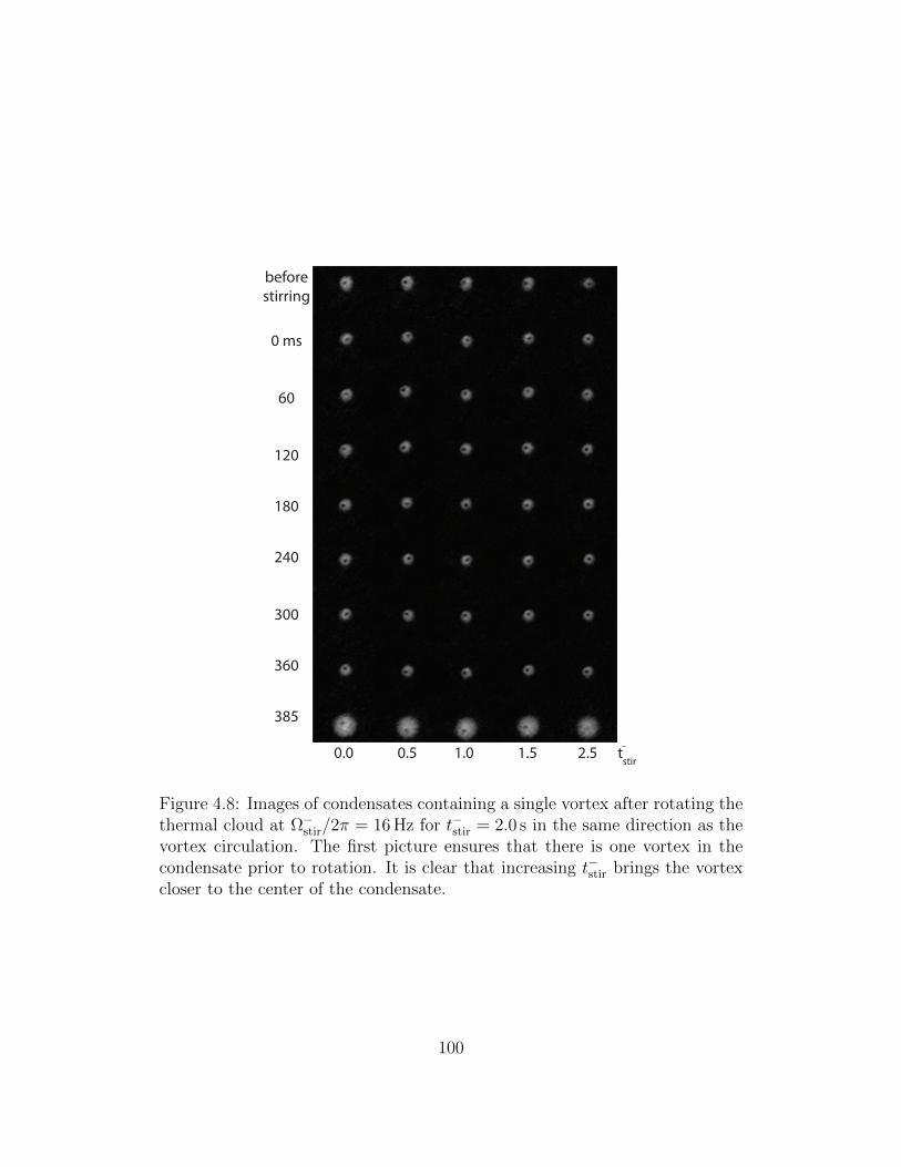
beforestirring

0 ms

60

120

180

240

300

360

385

0.0 0.5 1.0 1.5 2.5 t-stir

Figure 4.8: Images of condensates containing a single vortex after rotating thethermal cloud at Ω−stir/2π = 16 Hz for t−stir = 2.0 s in the same direction as thevortex circulation. The first picture ensures that there is one vortex in thecondensate prior to rotation. It is clear that increasing t−stir brings the vortexcloser to the center of the condensate.

100

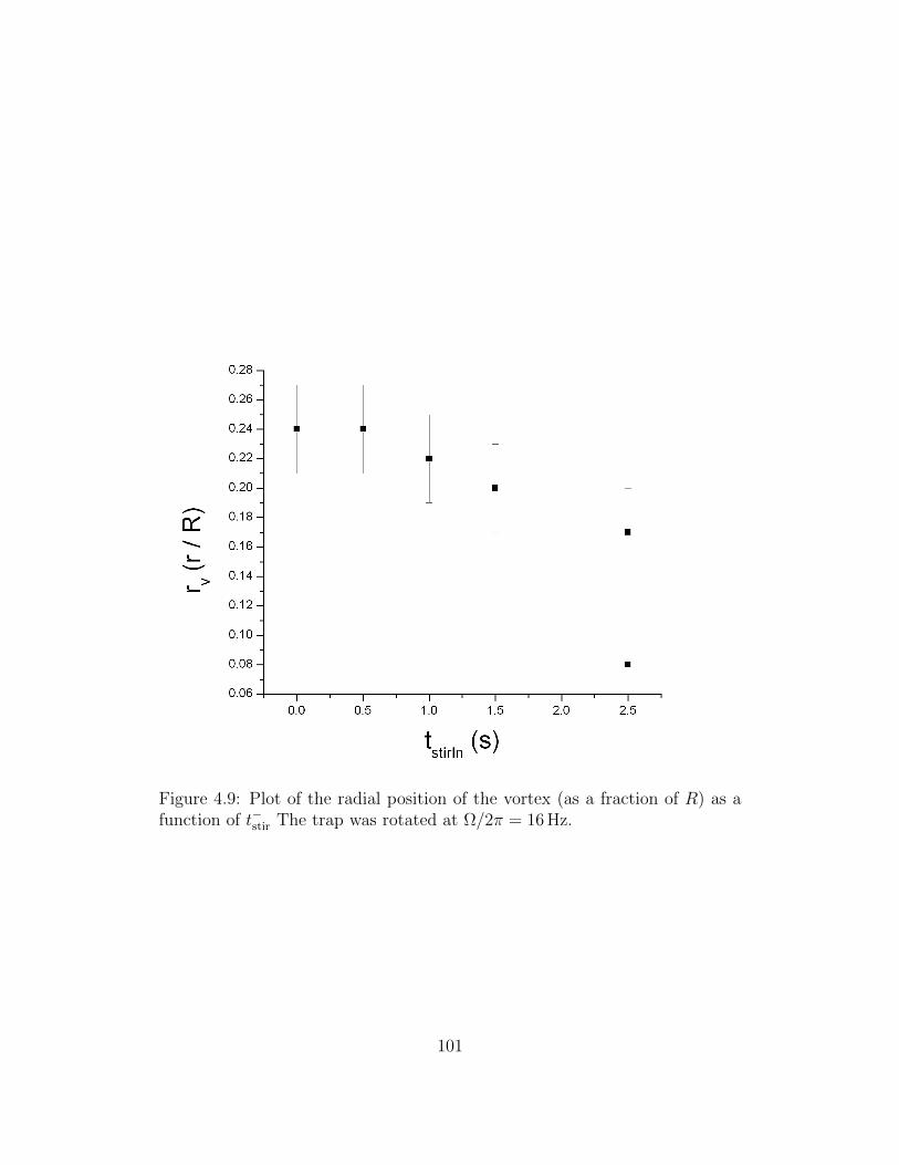
Figure 4.9: Plot of the radial position of the vortex (as a fraction of R) as afunction of t−stir The trap was rotated at Ω/2π = 16 Hz.

101

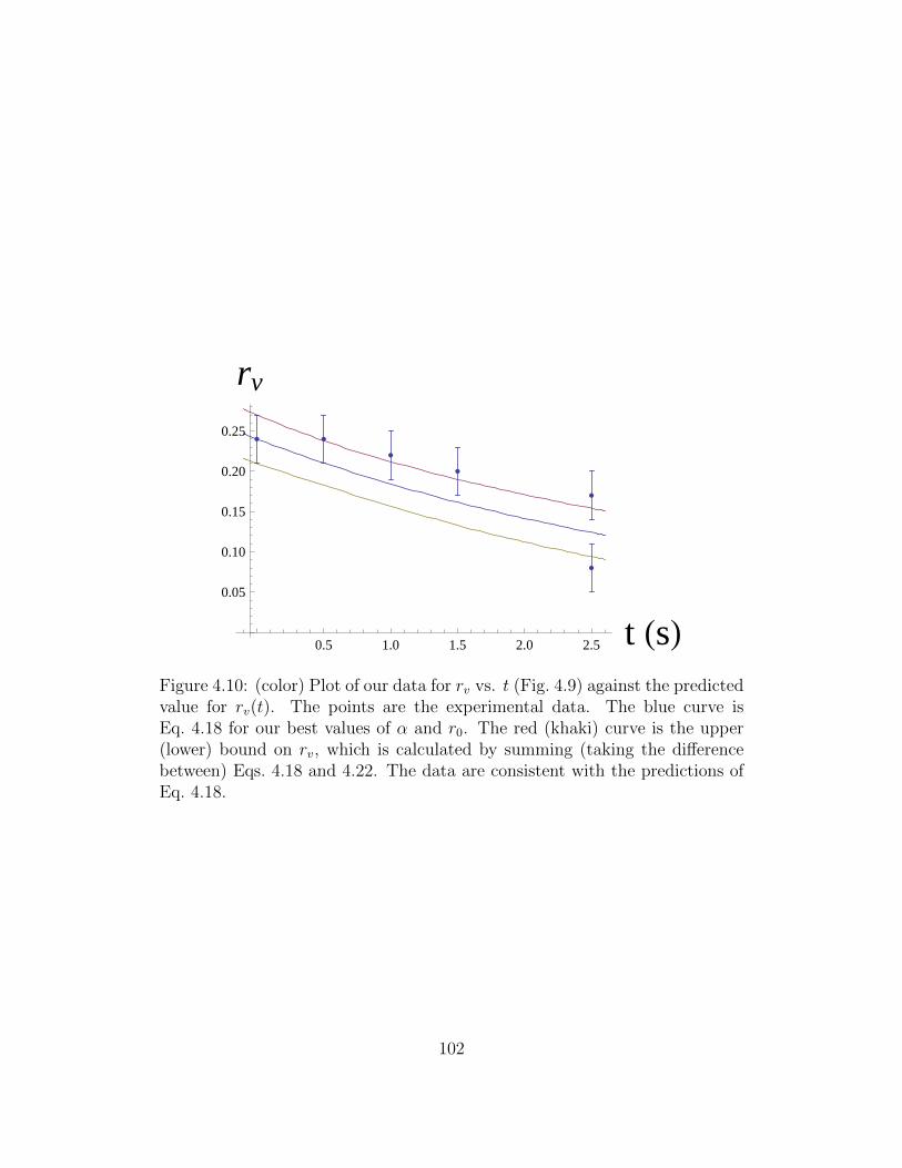
0.5 1.0 1.5 2.0 2.5 t HsL0.05

0.10

0.15

0.20

0.25

rv

Figure 4.10: (color) Plot of our data for rv vs. t (Fig. 4.9) against the predictedvalue for rv(t). The points are the experimental data. The blue curve isEq. 4.18 for our best values of α and r0. The red (khaki) curve is the upper(lower) bound on rv, which is calculated by summing (taking the differencebetween) Eqs. 4.18 and 4.22. The data are consistent with the predictions ofEq. 4.18.

102

beforestirring

0 ms

60

120

180

240

300

360

385

Figure 4.11: Images of condensates containing multiple vortices after rotatingthe thermal cloud at Ωstir/2π = 20 Hz and ε = 0.102 for tstir = 2.0 s in the samedirection as the vortex circulation. The first picture determines the numberof vortices in the condensate prior to rotation. It is clear that rotating thethermal cloud in the same direction as the vortex circulation results in theformation of a lattice.

103

anism by which a single vortex moves to the center of the condensate in the

presence of a thermal cloud rotating at positive Ωstir (Section 4.1): the col-

lisions increase the angular momentum of the condensate, with a maximum

value that depends on the number of pre-existing vortices. The vortex config-

uration that maximizes angular momentum is a triangular lattice, consistent

with our observations [61]. Once the vortices have formed a lattice, the an-

gular momentum cannot be increased without the introduction of additional

vortices, which requires the presence of a dynamical instability (Sec. 3.2.2).

We next consider Ωstir < 0, i.e., the thermal cloud is rotated in the opposite

direction of the vortex circulation. The vortices are initially in a lattice con-

figuration, generated by the process described above. What we observe after

rotating the thermal cloud depends sharply on the initial number of vortices.

If there are two vortices, we observe that one vortex moves to the center of the

condensate while the other exits the condensate within the first 900 ms. Then,

the vortex that has moved to the center begins to leave the condensate as well

(as in Sec. 4.2.2), and is displaced well towards the edge of the condensate

after 1800 ms. Figure 4.12 shows images of condensates taken after rotating

for various tstir at Ωstir/2π = −15 Hz.

When there are initially three vortices, two vortices exit the condensate at

first, while the third moves to the center. The two vortices disappear after

∼ 800 ms of rotation. The third vortex then begins to leave the condensate.

Figure 4.13 shows images taken after rotating for various tstir at Ωstir/2π =

−15 Hz.

The process of ‘stirring out’ multiple vortices may be understood most

104

1st EarlyPicture

2nd EarlyPicture

0 ms

60

120

180

240

300

325

0.4 0.6 0.8 0.9 1.5 1.8 tstir

Figure 4.12: Images of condensates containing two vortices after rotating thethermal cloud at Ωstir/2π = −15 Hz and ε = 0.102 in the direction oppositeto the vortex circulation. The first picture is taken to determine the numberof vortices in the condensate prior rotation. The second picture is taken afterthe procedure that forces the vortices into a lattice configuration. In the first0.9 s we observe that one vortex exits the condensate while the other movestowards the center. The remaining vortex then moves outwards.

105

1st EarlyPicture

2nd EarlyPicture

0 ms

60

120

180

240

300

325

0.4 0.5 0.7 0.8 0.9 tstir

Figure 4.13: Images of condensates containing three vortices after rotating thethermal cloud at Ωstir/2π = −15 Hz and ε = 0.102 in the direction oppositeto the vortex circulation. The first picture is taken to determine the numberof vortices in the condensate prior rotation. The second picture is taken afterthe procedure that forces the vortices into a lattice configuration. In the first0.8 s we observe that two vortices exit the condensate while the other movestowards the center. The remaining vortex then moves outwards.

106

easily if we compare it to the process of ‘stirring in’ vortices described earlier in

this section. In the latter case, angular momentum is added to the condensate

until it reaches a maximum value determined by the initial number of vortices

in the condensate. In the former case, angular momentum is removed from the

condensate. The minimum angular momentum of the condensate (zero) can be

achieved by continuously reducing the angular momentum, independent of the

number of initial vortices. The difference is that, while a dynamical instability

is required for the entrance of vortices, there is no such requirement for the

exit of vortices.

In our observations (Figs. 4.12 and 4.13), the first step in this continuous

removal of angular momentum is a transition from the state in which angular

momentum is maximized for n vortices (a lattice) to the state in which angular

momentum is maximized for a single vortex (a single vortex in the center

of the condensate). This is accomplished by the coincidence of the exit of

n − 1 vortices with the movement of one ‘remnant’ vortex to the center of

the condensate. After the first n− 1 vortices exeunt, the remnant vortex also

exits, and the angular momentum of the condensate ultimately drops to zero.

Continued rotation of the thermal cloud, however, is insufficient to induce

condensate rotation in the opposite direction. This is, again, a consequence of

the inability to introduce vortices to the condensate in absence of a dynamical

instability.

107

Chapter 5

Observations of

Counter-Circulating Vortices

The experimental study of counter-circulating vortex clusters is an important

step on the path to understanding quantum turbulence (QT). This requires

the generation of condensates containing two or more counter-circulating vor-

tices. In this chapter we define this counter-circulating condition in terms of

vortices and antivortices, where vortices are vortex lines with one sense of cir-

culation (say, CCW), and antivortices have the opposite sense of circulation

(CW). With the notable exception of vortex dipoles, spontaneous generation of

vortex-antivortex clusters has not yet been observed in a BEC [8, 9]. We can,

however, ‘artificially’ generate counter-circulating vortices through judicious

use of the techniques developed in the previous two chapters.

In Section 5.1 we describe how we generate condensates containing two,

three, or four counter-circulating vortices. We then present images illustrat-

108

ing the resulting behavior. Section 5.2 presents observations of condensates

in which vortices abruptly disappear from the condensate. Although the loss

mechanism is not yet clear, it is intriguing to imagine that these events cor-

respond to vortex-antivortex reconnection or annihilation events, which are

intrinsic to quantum turbulence since these events are required for the ‘untan-

gling’ of the vortex tangle.

5.1 Generation and Observation of Vortex-Antivortex

Clusters

The following procedure generates condensates with two or more counter-

circulating vortices. Throughout, positive Ω corresponds to rotating the trap

counter-clockwise (CCW).

1. Generate a CCW vortex — Using the method of Sec. 3.1 with ε = 0.194,

create a vortex with CCW circulation. The RF shield power is then

reduced by 14.35 dB, and the frequency increased by 0.3 MHz, which

permits the formation of a thermal cloud. The power reduction is es-

sential for reasons that are not well understood. If it is not reduced,

however, we obtain a vortex lattice (Fig. 5.1(e)) rather than a cluster of

counter-circulating vortices (Fig. 5.1(d)) at the conclusion of the proce-

dure.

2. ‘Stir in’ the vortex — Push the vortex to the center of the condensate by

rotating the thermal cloud CCW (ε = 0.102, tcenter = 2.0 s, Ωcenter/2π =

109

15 Hz; Sec. 4.2.1). We push the vortex towards the center so that it is

not ‘stirred out’ (Sec. 4.2.2) during the following steps, which rely on

rotating the trap clockwise (CW). The shield frequency is then restored

to its usual value to reduce the temperature of the sample.

3. Generate antivortices — Generate CW circulating vortices by driving the

counter-rotating quadrupole mode (ε = 0.010, tquad = 1.5 s, Ωquad/2π =

−25 Hz; Sec. 3.3.2). This generates CW vortices at the outer reaches of

the condensate. Once again, a thermal cloud is formed by increasing the

shield frequency by 0.30 MHz.

4. Stir in the antivortices — Push the CW circulating vortices towards the

center of the condensate by rotating the trap CW (ε = 0.102, t−stir = 1.0 s,

Ω−stir/2π = −15 Hz; Sec. 4.3). This step yields a variety of interesting

counter-circulating configurations beyond that of a single CCW vortex at

the center and multiple CW vortices near the edge. The trap symmetry

is then restored (ε = 0.0), as is the shield frequency, which once again

reduces the temperature of the sample.

5. Image the condensate — Take a series of images of the condensate by

repeatedly extracting, releasing, and imaging 5% of the atoms from the

trap (Sec. 2.2.5).

Figure 5.1 shows image sequences of different condensates taken after each

step of this procedure.

We can reliably generate condensates containing two, three, and four counter-

circulating vortices in this way. The three vortex configuration is by far the

110

a b c d e

Figure 5.1: Images of a condensate after each process in the counter-circulationgeneration procedure. These images are all of different condensates. (a) Westart with a condensate containing a CCW circulating vortex at some r0. (b)We push that vortex to the center. (c) We generate CW circulating vorticeson the outside of the condensate. (d) Pushing the CW circulating vorticestowards the center of the condensate generates observable counter-circulatingbehavior. Notice that the two vortices on the outside precess CW while theone on the inside precesses CCW. (e) If we do not reduce the RF Shieldspower after evaporation, exciting the quadrupole mode (step 3) generates acondensate with a CW vortex lattice.

111

most commonly observed. In the case of four vortices, we have to this date

only been able to generate the configuration with three vortices of one sense

of circulation and one vortex of the other sense. Figures 5.2, 5.3, and 5.4 show

image sequences of two, three, and four counter-circulating vortices, respec-

tively.

5.2 Disappearance of Counter-Circulating Vor-

tices

We also have discovered a different, albeit less well understood, process that

results in the generation of counter-circulating vortex clusters. The procedure

is the same as the one described in the previous section, except in step 1 we

stir in more than one CCW vortex by rotating at Ω/2π = 11 Hz and we do

not reduce the shield’s power. We also replace steps 2—4 with the following

two steps:

2. Stir in the vortex : Keeping ε = 0.192, we push the vortices to the center

by rotating the thermal cloud CCW at Ωcenter/2π = 11 Hz for tcenter =

1.0 s.

3. Reverse direction of thermal cloud : We immediately reverse the direction

of the thermal cloud rotation by rotating the trap at Ωstir/2π = −12.5 Hz

for tstir = 0.2 s. Surprisingly, antivortices are generated during this step

by a mechanism that is not yet understood. It is possible that the im-

mediate reversal of direction creates a dynamical instability from which

112

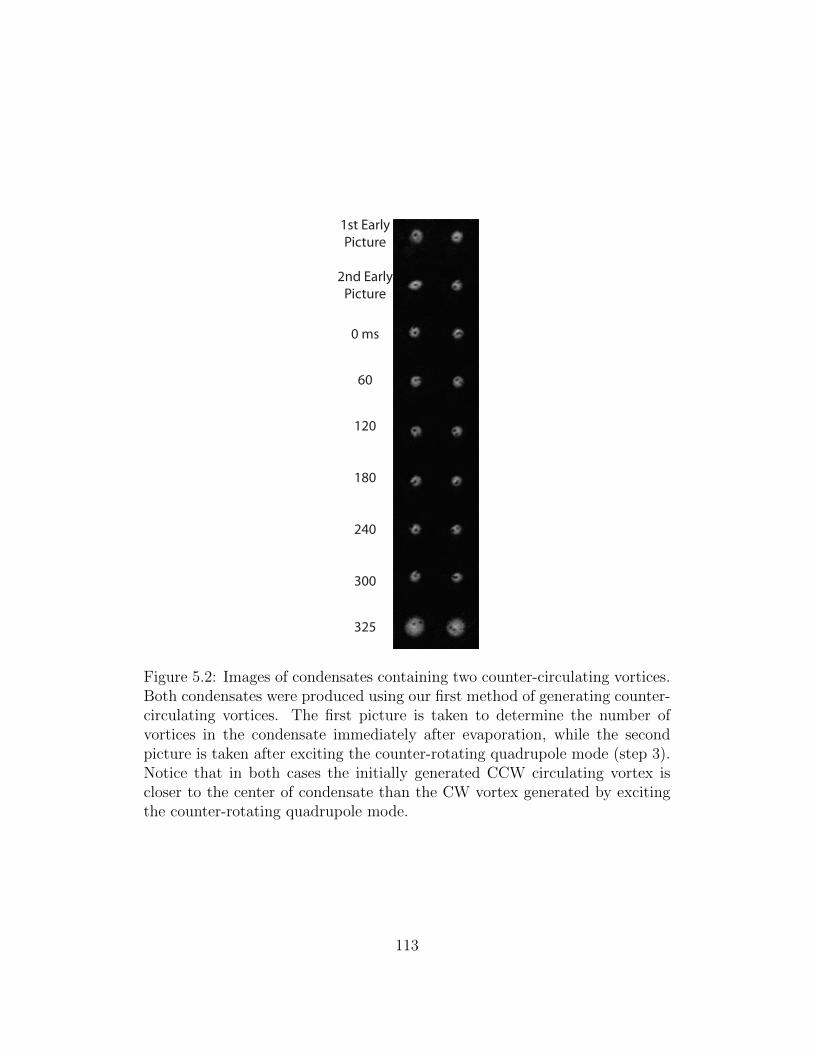
1st EarlyPicture

2nd EarlyPicture

0 ms

60

120

180

240

300

325

Figure 5.2: Images of condensates containing two counter-circulating vortices.Both condensates were produced using our first method of generating counter-circulating vortices. The first picture is taken to determine the number ofvortices in the condensate immediately after evaporation, while the secondpicture is taken after exciting the counter-rotating quadrupole mode (step 3).Notice that in both cases the initially generated CCW circulating vortex iscloser to the center of condensate than the CW vortex generated by excitingthe counter-rotating quadrupole mode.

113

1st EarlyPicture

2nd EarlyPicture

0 ms

60

120

180

240

300

325

Figure 5.3: Images of condensates containing three counter-circulating vor-tices. Both condensates were produced using our first method of generatingcounter-circulating vortices. The first picture is taken to determine the numberof vortices in the condensate immediately after evaporation, while the secondpicture is taken after exciting the counter-rotating quadrupole mode (step 3).Notice that in all cases the initially generated CCW circulating vortex is closerto the center of condensate than the two CW vortices generated by excitingthe counter-rotating quadrupole mode.

114

1st EarlyPicture

2nd EarlyPicture

0 ms

60

120

180

240

300

325

Figure 5.4: Images of condensates containing four counter-circulating vortices.Both condensates were produced using our first method of generating counter-circulating vortices. The first picture is taken to determine the number ofvortices in the condensate immediately after evaporation, while the secondpicture is taken after exciting the counter-rotating quadrupole mode (step 3).Notice that in both cases the initially generated CCW circulating vortex iscloser to the center of condensate than the three CW vortices generated byexciting the counter-rotating quadrupole mode.

115

vortex generation can occur. Rotating the trap at a relatively high dis-

tortion (ε = 0.192) may in fact result in vortex generation through an off

resonant (Ωquad/2π ≈ 0.707 · ωr/2π = 25.7 Hz) quadrupole mode excita-

tion [11, 12]. Whatever the mechanism, we image the condensate after

restoring the trap symmetry (ε = 0.0) and the shield frequency in order

to reduce the temperature of the sample.

Interestingly, the counter-circulating vortices produced by this method oc-

casionally disappear in the middle of the imaging sequence (Fig. 5.5(a)). The

procedure described in the previous section also generates condensates which

exhibit this ‘lossy’ behavior, although far more rarely (Fig. 5.5(b)). In the con-

densates shown in Fig. 5.5 we clearly observe the disappearance of vortices in

between images. Given that the images are spaced by 0.06 s, this phenomenon

explaining the disappearance must occur over a timescale below 0.06 s. The

disappearance of a vortex typically occurs as it precesses near the edge of the

condensate. However, the time it takes a vortex to move to the edge of the

condensate is on the order of tens of seconds (Sec. 4.2.2). The disparity of two

orders of magnitude between the timescales implies that these disappearances

must be caused by some other phenomenon.

Two phenomena that fit this description are pair annihilation and vortex

reconnection. In pair annihilation events, vortices of the opposite sense col-

lide with each other and annihilate over a time period on the order of 0.1 s

or less [62–64]. During the annihilation process, the energy associated with

the vortex-antivortex pair is released through sound waves [63]. On the other

hand, in vortex reconnection events, vortices of the opposite circulation con-

116

nect and rotate such that they are no longer aligned with the z-axis, becoming

invisible by absorptive imaging [65, 66]. This process is believed to occur

over a timescale on the order of 0.010 s for vortices in a BEC with our trap

parameters [66].

It would be interesting to pursue the four methods of generating vortex-

antivortex clusters (the two discussed in this chapter, the excitation of the

counter-rotating quadrupole mode discussed in Section 3.3.2, and the simul-

taneous excitation of the m = ±2 quadrupole modes discussed in Section 3.4)

further, in order to determine a procedure that reliably produces condensates

with a few counter-circulating vortices near the center of the condensate. Such

a method could lead to a number of interesting experiments. For example, we

could answer the question of what happens when one rotates the thermal

cloud surrounding a condensate containing counter-circulating vortices. The

results of such an experiment may inform us of a method by that we can radi-

ally translate counter-circulating vortices such that their collision is inevitable.

This would give us a way to further study the possible pair annihilation and/or

vortex recombination events observed in Fig. 5.5.

It would also be interesting to determine a procedure that can produce

stable counter-circulating configurations, as observed in Ref. [67], since de-

termining the stability conditions of counter-circulating vortices provides a

window into the vortex-antivortex interactions which characterize quantum

turbulence [3].

117

0 ms

60

120

180

240

300

360

420

445

a1st EarlyPicture

2nd EarlyPicture

0 ms

60

120

180

240

300

325

b

Figure 5.5: Images in which several vortices disappear at once. Initially thecondensates contain two or more vortices. Then, during the image sequence,some of the vortices disappear. By the end, either one or zero vortices remain.(a) Images of condensates generated using the process discussed in this section.(b) This image is of a condensate generated using the process discussed in theprevious section. As we can see from the last two images, these disappear-ances can occur over time periods as brief as 25 ms. The first picture is takento determine the number of vortices in the condensate immediately after evap-oration, while the second picture is taken after exciting the counter-rotatingquadrupole mode.

118

Chapter 6

Conclusion

We have finally arrived at the end of our journey. Buttressed by our greater

understanding of the mechanisms by which we can generate and manipulate

quantized vortices, we observed interesting counter-circulating dynamics in

Bose-Einstein condensates (BECs), including possible pair annihilation and/or

vortex recombination events. We have moved vortex lines inward and outward

by juggling angular momentum between the condensate and a rotating ther-

mal population. This in particular is worthy of future study, since very little

research has been done on condensate-thermal cloud interactions. Indeed, we

know little of the effect a rotating thermal cloud might have on a condensate

that contains multiple counter-circulating vortices. We have done little more

than to identify and sketch any of these topics.

The use of extraction imaging provides the opportunity to observe the

state of the condensate without destroying it, which has been critical in the

development of a technique for generating counter-circulating vortices. The

119

knowledge that we have a condensate that initially contains a single vortex

with a known sense of circulation, for example, allows us to generate — and

to know that we have generated — counter-circulating vortices. Absent of a

method to push these antivortices towards the center of the condensate, we

would only be able to observe widely separated vortex-antivortex systems —

hardly a promising scenario for understanding the underlying dynamics.

Rotating the thermal cloud also leads to additional surprises. If in the

same direction as the vortex circulation, it causes a transition of the vortex

cores from a disordered ensemble to a lattice structure near the center of

the condensate. In the opposite direction, it results in the gradual removal

of vortices from the condensate over a time period of ∼ 2 s in an unusual

way: one vortex line moves to the center of the trap until the others depart.

This unexpected behavior allows us to move anti-vortex lines circulating in

one direction towards the center of the trap while maintaining a vortex line,

leading to a more diverse set of counter-circulating vortex configurations.

The reliable generation of condensates containing counter-circulating vor-

tices allows for the analysis of the fascinating dynamics of vortex-antivortex

interactions. Future work will center on the generation of interesting interac-

tions between counter-circulating vortices, such as pair annihilation and vortex

recombination. Analysis of such interactions will provide much-needed insight

into the nature of quantum turbulence, since the hallmark of quantum turbu-

lence is the existence of vortex tangles in which these interactions are common.

Quantum turbulence, in turn, is a more tractable problem than the notoriously

intractable problem of classical turbulence. Solving the problem of quantum

120

turbulence could result in valuable insight into classical turbulence, a problem

which has vexed scientists from da Vinci to Feynman.

121

Appendix A

Derivation of Hydrodynamic

Equations

This appendix presents derivations of the hydrodynamic equations for the

density and the velocity field of a BEC, reproduced here:

∂n

∂t+∇ · (nv) = 0 (A.1)

m∂v

∂t= −∇

(µ+

1

2mv2

)(A.2)

where

µ = V + nU0 −h2

2m√n∇2√n (A.3)

where V is the potential, m is the mass of 87Rb, and U0 = 4πh2a/m.

I will be following the method of Pethick and Smith [1] to derive the above

122

equations. To derive Eq. A.1 we start with the Gross-Pitaevskii equation,

− h2

2m∇2ψ (r, t) + V (r)ψ (r, t) + U0 |ψ (r, t)|2 ψ (r, t) = ih

∂ψ (r, t)

∂t, (A.4)

then we multiply both sides by ψ∗ (r, t) and subtract the complex conjugate

of the ensuing equation, which eliminates all terms dependent on V and U0,

yielding

h

2m

[ψ∇2ψ∗ − ψ∗∇2ψ

]= i

[ψ∗∂ψ

∂t+ ψ

∂ψ

∂t

]. (A.5)

We can rewrite Eq. A.5 using product rules:

∂ |ψ|2

∂t+∇ ·

[h

2mi(ψ∗∇ψ − ψ∇ψ∗)

]= 0, (A.6)

yielding a formula in the form of a continuity equation (i.e. Eq. A.1)

∂n

∂t+∇ · (nv) = 0. (A.7)

where n = |ψ|2 and

v =h

2mi

(ψ∗∇ψ − ψ∇ψ∗)|ψ|2

(A.8)

In order to derive Eq. A.2 we start with assuming that ψ = feiφ and then

we substitute ψ = feiφ into Eq A.4. Since

i∂ψ

∂t= i

∂f

∂teiφ − ∂φ

∂tfeiφ (A.9)

123

and

−∇2ψ =[−∇2f + (∇φ)2 f − i∇2φf − 2i∇φ · ∇f

]eiφ, (A.10)

substituting ψ = feiφ into Eq A.4 and taking the real part yields

−h∂φ∂t

= − h2

2mf∇2f +

1

2mv2 + V (r) + U0f

2, (A.11)

while taking the imaginary part yields (after utilizing the product rule)

∂ (f 2)

∂t= − h

m∇ ·(f 2∇φ

). (A.12)

Eq. A.12 is the continuity equation, Eq. A.7, expressed in terms of f and φ.

In order to get the hydrodynamic equation for the velocity of the BEC, where

velocity is given by

v =h

m∇φ, (A.13)

we must take the gradient of Eq. A.11 yielding Eq. A.2, reproduced below

m∂v

∂t= −∇

(µ+

1

2mv2

), (A.14)

where µ is given by Eq. A.3.

124

Bibliography

[1] C. J. Pethick and H. Smith, Bose-Einstein Condensation in Dilute Gases

(Cambridge University Press, 2008), 2nd ed.

[2] M. H. Anderson, J. R. Ensher, M. R. Matthews, C. E. Wie-

man, and E. A. Cornell, “Observation of Bose-Einstein Conden-

sation in a Dilute Atomic Vapor,” Science 269, 198 (1995),

http://www.sciencemag.org/content/269/5221/198.full.pdf, URL

http://www.sciencemag.org/content/269/5221/198.abstract.

[3] M. Tsubota, “Quantum turbulence: From superfluid helium to atomic

Bose-Einstein condensates,” J. Phys. Con. Matt. 21, 164207 (2009).

[4] J. Maurer and P. Tabeling, “Local investigation of superfluid

turbulence,” EPL (Europhysics Letters) 43, 29 (1998), URL

http://stacks.iop.org/0295-5075/43/i=1/a=029.

[5] S. R. Stalp, L. Skrbek, and R. J. Donnelly, “Decay of Grid Turbulence in

a Finite Channel,” Phys. Rev. Lett. 82, 4831 (1999).

[6] L. Skrbek, J. J. Niemela, and R. J. Donnelly, “Four Regimes of Decaying

Grid Turbulence in a Finite Channel,” Phys. Rev. Lett. 85, 2973 (2000).

125

[7] S. Watch, “Stanford University’s George Papanicolaou Seeks Order in

Turbulence,” (2008).

[8] D. F. Freilich, “Real-Time Experimental Visualization of Bose-Einstein

Condensates with One and Two Vortices,” Undergraduate Thesis,

Amherst College (2010).

[9] D. V. Freilich, D. M. Bianchi, A. M. Kaufman, T. K. Langin, , and D. S.

Hall, “Real-Time Dynamics of Single Vortex Lines and Vortex Dipoles in

a Bose-Einstein Condensate,” Science 329, 1128 (2010).

[10] K. W. Madison, F. Chevy, W. Wohlleben, and J. Dalibard, “Vortex For-

mation in a Stirred Bose-Einstein Condensate,” Phys. Rev. Lett. 84, 806

(2000).

[11] K. W. Madison, F. Chevy, V. Bretin, , and J. Dalibard, “Stationary States

of a Rotating Bose-Einstein Condensate: Routes to Vortex Nucleation,”

Phys. Rev. Lett. 86, 4443 (2001).

[12] E. Hodby, G. Hechenblaikner, S. A. Hopkins, O. M. Marag, and C. J. Foot,

“Vortex Nucleation in Bose-Einstein Condensates in an Oblate, Purely

Magnetic Potential,” Phys. Rev. Lett. 88, 010405 (2001).

[13] P. C. Haljan, I. Coddington, P. Engels, and E. Cornell, “Driving Bose-

Einstein-Condensate Vorticity with a Rotating Normal Cloud,” Phys.

Rev. Lett. 87, 210403 (2001).

[14] J. R. Abo-Shaeer, C. Raman, J. M. Vogels, and W. Ketterle, “Observa-

126

tion of Vortex Lattices in Bose-Einstein Condensates,” Science 292, 746

(2001).

[15] C. N. Weiler, T. W. Neely, D. R. Scherer, A. S. Bradley, M. J. Davis, and

B. P. Anderson, “Spontaneous vortices in the formation of Bose-Einstein

condensates,” Nature 455, 948 (2008).

[16] T. W. Neely, E. C. Samson, A. S. Bradley, M. J. Davis, and B. P. Ander-

son, “Observation of Vortex Dipole in an Oblate Bose-Einstein Conden-

sate,” Phys. Rev. Lett. 104, 160401 (2010).

[17] E. A. L. Henn, J. A. Seman, G. Roati, K. M. F. Magalhaes, and V. S.

Bagnato, “Emergence of Turbulence in an Oscillating Bose-Einstein Con-

densate,” Phys. Rev. Lett. 103, 045301 (2009).

[18] J. A. Seman, E. A. L. Henn, R. F. Shiozaki, G. Roati, F. J.

Poveda-Cuevas, K. M. F. Magalhes, V. I. Yukalov, M. Tsubota,

M. Kobayashi, K. Kasamatsu, and V. S. Bagnato, “Route to turbu-

lence in a trapped Bose-Einstein condensate,” arXiv:1007.4953v3 [cond-

mat.quant-gas] (2011).

[19] D. V. Schroeder, Thermal Physics (Addison Wesley Longman, 2000).

[20] A. L. Fetter and A. A. Svidzinsky, “Vortices in a trapped dilute BoseE-

instein condensate,” J. Phys.: Condens. Matter 13, R135 (2001).

[21] A. M. Kaufman, “Radiofrequency Dressing of Atomic Feshbach Reso-

nances,” Undergraduate Thesis, Amherst College (2009).

127

[22] D. M. Bianchi, “Characterizing a Crossed-Beam Optical Dipole Trap for

Ultracold 87Rb Atoms,” Undergraduate Thesis, Amherst College (2009).

[23] M. L. Goldman, “Landau-Zener Transitions and a Feshbach Resonance

in Spinor Bose Einstein Condensates,” Undergraduate Thesis, Amherst

College (2008).

[24] E. S. Petrik, “Vortices in an Optically Trapped 87Rb Bose-Einstein Con-

densate,” Undergraduate Thesis, Amherst College (2008).

[25] D. H. Guest, “A Cross-Beam Far Off-Resonance Optical Trap for 87Rb

Bose-Einstein Condensates,” Undergraduate Thesis, Amherst College

(2007).

[26] J. Merrill, “Characterization of Inelastic Losses from Bose-Einstein Con-

densates in the | 2, 1〉 State of 87Rb,” Undergraduate Thesis, Amherst

College (2006).

[27] T. Menon, “Quantized Vortex Nucleation in a 87Rb Bose-Einstein Con-

densate,” Undergraduate Thesis, Amherst College (2005).

[28] M. H. Wheeler, “A New Observation of Matter-Wave Interference in Bi-

nary Bose-Einstein Condensates,” Undergraduate Thesis, Amherst Col-

lege (2004).

[29] T. J. Reber, “Creating and Optically Trapping a Bose-Einstein Conden-

sate of Rubidium 87,” Undergraduate Thesis, Amherst College (2003).

128

[30] S. F. Owen, “Magnetic Trapping for Bose-Einstein Condensation of

87Rb,” Undergraduate Thesis, Amherst College (2002).

[31] B. Samelson-Jones, “Making the Coldest Stuff in the Universe: Vacuum

Construction and Magneto-Optic Trapping for Bose-Einstein Conden-

sate,” Undergraduate Thesis, Amherst College (2001).

[32] N. J. Stokes, “Diode Laser Systems for Bose-Einstein Condensation,” Un-

dergraduate Thesis, Amherst College (2000).

[33] E. Arimondo, M. Inguscio, and P. Violino, “Experimental determinations

of the hyperfine structure in the alkali atoms,” Rev. Mod. Phys. 49, 31

(1977).

[34] D. A. Steck, “Rubidium 87 D Line Data,” Published Online (2008).

[35] C. Wieman, “The Richtmyer Memorial Lecture: Bose-Einstein Conden-

sationin an Ultracol Gas,” Am. J. Phys. 64, 847 (1996).

[36] S. Chu, J. E. Bjorkholm, A. Ashkin, , and A. Cable, “Experimental Ob-

servation of Optically Trapped Atoms,” Phys. Rev. Lett. 57, 314 (1986).

[37] H. Metcalf and P. van der Straten, Laser Cooling and Trapping (Springer,

Berlin, 1999).

[38] C. J. Myatt, N. R. Newbury, R. W. Ghrist, S. Loutzenhiser, and C. E.

Wieman, “Multiply loaded magneto-optical trap,” Optics Letters 21, 290

(1996).

129

[39] W. Petrich, M. Anderson, J. Ensher, and E. Cornell, “Behavior of atoms

in a compressed magneto-optical trap,” J. Opt. Soc. Am. B. 11, 1332

(1994).

[40] D. M. Brink and C. V. Sukumar, “Majorana spin-flip transitions in a

magnetic trap,” Phys. Rev. A. 74, 035401 (2006).

[41] W. Petrich, M. H. Anderson, J. R. Ensher, and E. A. Cornell, “Stable,

tightly confining magnetic trap for evaporative cooling of neutral atoms,”

Phys. Rev. Lett. 74, 3352 (1995).

[42] J. Ensher, The First Experiments with Bose-Einstein Condensation of

87Rb, Ph.D. thesis, University of Colorado (1998).

[43] J. Roberts, Bose-Einstein Condensates with Tunable Atom-atom Interac-

tions: The First Experiments with 85Rb BECs, Ph.D. thesis, University

of Colorado (2001).

[44] A. Siegman, Lasers (University Science Books, 1986).

[45] P. Rosenbusch, D. Petrov, S. Sinha, F. Chevy, V. Bretin, Y. Castin,

G. Shlyapnikov, and J. Dalibard, “Critical rotation of a harmonically

trapped Bose gas,” Phys. Rev. Lett. 88, 250403 (2002).

[46] N. Parker and C. Adams, “Emergence and Decay of Turbulence in Stirred

Atomic Bose-Einstein Condensates,” Phys. Rev. Lett. 95, 145301 (2005).

[47] S. Sinha and Y. Castin, “Dynamic Instability of a Rotating Bose-Einstein

Condensate,” Phys. Rev. Lett. 87, 190402 (2001).

130

[48] K. Kasamatsu, M. Tsubota, and M. Ueda, “Nonlinear dynamics of vortex

lattice formation in a rotating Bose-Einstein condensate,” Phys. Rev. A.

67, 033610 (2003).

[49] M. Tsubota, K. Kasamatsu, and M. Ueda, “Vortex lattice formation in a

rotating Bose-Einstein condensate,” Phys. Rev. A 65, 023603 (2002).

[50] N. G. Parker, R. M. W. van Bijnen, and A. M. Martin, “Instabilities

leading to vortex lattice formation in rotating Bose-Einstein condensates,”

Phys. Rev. A. 73, 061603 (2006).

[51] A. Recati, F. Zambelli, , and S. Stringari, “Overcritical Rotation of a

Trapped Bose-Einstein Condensate,” Phys. Rev. Lett. 86, 377 (2001).

[52] T. W. B. Kibble, “Topology of cosmic domains and strings,” J. Phys. A.

9, 1387 (1976).

[53] W. H. Zurek, “Cosmological experiments in superfluid helium?” Nature

(London) 317, 505 (1985).

[54] W. H. Zurek, “Cosmological experiments in condensed matter systems,”

Phys. Rep. 276, 177 (1996).

[55] F. Chevy, K. Madison, and J. Dalibard, “Measurement of the Angular

Momentum of a Rotating Bose-Einstein Condensate,” Phys. Rev. Lett.

85, 225 (2000).

[56] F. Zambelli and S. Stringari, “Quantized Vortices and Collective Oscilla-

131

tions of a Trapped Bose-Einstein Condensate,” Phys. Rev. Lett. 81, 1754

(2001).

[57] G. Sagnac, “On the proof of the reality of the luminiferous aether by the

experiment with a rotating interferometer,” Comptes Rendus 157, 1410

(1913).

[58] B. Jackson, N. P. Proukakis, C. F. Barenghi, and E. Zaremba, “Finite-

temperature vortex dynamics in Bose-Einstein condensates,” Phys. Rev.

A. 79, 053615 (2009).

[59] K. Schwarz, “Three-dimensional vortex dynamics in superfluid 4He: Line-

line and line-boundary interactions,” Phys. Rev. B. 31, 5782 (1985).

[60] B. Anderson, P. Haljan, C. Wieman, and E. Cornell, “Vortex Precession in

Bose-Einstein Condensates: Observations with Filled and Empty Cores,”

Phys. Rev. Lett. 835, 2587 (2000).

[61] D. Butts and D. Rokhsar, “Predicted signatures of rotating Bose-Einstein

condensates,” Nature 397, 327 (1999).

[62] A. Klein, D. Jaksch, Y. Zhang, and W. Bao, “Dynamics of vortices in

weakly interacting Bose-Einstein condensates,” Phys. Rev. A 76, 043602

(2007).

[63] J. Ruostekoski and Z. Dutton, “Engineering vortex rings and systems for

controlled studies of vortex interactions in Bose-Einstein condensates,”

Phys. Rev. A 72, 063626 (2005).

132

[64] S.-i. Ogawa, M. Tsubota, and Y. Hattori, “Study of Reconnection and

Acoustic Emission of Quantized Vortices in Superfluid by the Numerical

Analysis of the GrossPitaevskii Equation,” J. Phys. Soc. Jpn. 71, 813

(2002).

[65] J. Koplik and H. Levine, “Vortex reconnection in superfluid helium,”

Phys. Rev. Lett. 71, 1375 (1993).

[66] H. Takeuchi, K. Kasamatsu, and M. Tsubota, “Spontaneous radiation

and amplification of Kelvin waves on quantized vortices in Bose-Einstein

condensates,” Phys. Rev. A 79, 033619 (2009).

[67] J. A. Seman, E. A. L. Henn, M. Haque, R. F. Shiozaki, E. R. F. Ramos,

M. Caracanhas, P. Castilho, C. Castelo Branco, P. E. S. Tavares, F. J.

Poveda-Cuevas, G. Roati, K. M. F. Magalhaes, et al., “Three-vortex

configurations in trapped Bose-Einstein condensates,” Phys. Rev. A 82,

033616 (2010).

133