the counter-rotating vortex pair in film-cooling …...the counter-rotating vortex pair in...

The Counter-Rotating Vortex Pair in Film-Cooling Flow and

its Effect on Cooling Effectiveness

Haoming Li

A Thesis

in

The Department

Of

Mechanical and Industrial Engineering

Presented in Partial Fulfillment of the Requirements

for the Degree of Master of Applied Science (Mechanical Engineering) at

Concordia University

Montreal, Quebec, Canada

December 2011

©Haoming Li, 2011

iii

ABSTRACT

The Counter-Rotating Vortex Pair in Film-Cooling

Flow and its Effect on Cooling Effectiveness

Haoming Li

A fundamental investigation on a key vortical structure in film cooling flow, which is

called counter-rotating vortex pair (CRVP), has been performed. Traditionally, the

coolant’s momentum flux ratio is thought as the most critical parameter on film cooling

effectiveness, which is the index of film cooling performance, and this performance is

also influenced notably by CRVP. About the sources of CRVP, the in-tube vortex, the in-

tube boundary layer vorticity, the jet/mainstream interaction effect, alone or combined,

are proposed as the main source in the literature. A numerical approach was applied in

present study. By simulating a general inclined cylindrical cooling hole on a flat plate

(the baseline case), the CRVP was visualized as well as the in-tube vortex. Another case,

which is identical with the baseline except the boundary condition of the in-tube wall was

set as free-slip to isolate its boundary layer effect, was simulated for comparing. Their

comparisons have clarified that the jet/mainstream interaction is the only essential source

of CRVP. Through further analyzing its mechanism, CRVP was found to be a pair of x

direction (mainstream wise direction) vortices. Hence, the velocity gradients -v/z and

w/y were the promoters of CRVP. Applying this mechanism, a new scheme named

nozzle scheme was designed to control the CRVP intensity and isolate the overall

momentum flux ratio Iov, a parameter used in literature. Analysis of the effects of CRVP

iv

intensity and momentum flux ratio on film cooling effectiveness has demonstrated that

the CRVP intensity, instead of the momentum flux ratio, was the most critical factor

governing the film cooling performance.

v

Table of Contents

List of Figures ................................................................................................ vi

List of Tables ................................................................................................ vii

Nomenclature ................................................................................................. ix

1 Introduction ................................................................................................... 1

2 Literature Review ......................................................................................... 3

2.1 Previous Investigations ........................................................................................... 3

2.2 Summary of the Literature ...................................................................................... 7

2.3 Objectives and Contributions .................................................................................. 8

3 Methodology and Mathematical Modeling ................................................10

3.1 Numerical Model .................................................................................................. 10

3.1.1 Conservation Equations ................................................................................ 10

3.1.2 Turbulence Modeling .................................................................................... 11

3.1.3 The Standard Wall Functions........................................................................ 13

3.2 Geometries and Boundary Conditions .................................................................. 15

3.3 Parameter Definitions ........................................................................................... 17

3.4 Configurations of the Nozzle Scheme .................................................................. 19

3.5 Test Matrix ............................................................................................................ 20

3.6 Grid Independence and Validation ....................................................................... 22

4 The Formation of Counter-Rotating Vortex Pair

in Film-Cooling Flow and its Mechanism ................................................25

vi

4.1 Formation of the CRVP ........................................................................................ 25

4.2 The Mechanism of CRVP’s Formation ................................................................ 29

4.3 The Effect of The in-Tube Boundary Layer ......................................................... 34

4.4 The CRVP Characters in Film-Cooling Flow

Contrasting With Those in JICF ........................................................................... 36

5 The Effects of Counter-Rotating Vortex Pair

Intensity on Film-Cooling Effectiveness ..................................................38

5.1 The Effect of Nozzle Scheme on CRVP ............................................................... 38

5.2 The Film-Cooling Effectiveness of the Nozzle

Schemes and the Effect of CRVP Intensity .......................................................... 43

5.3 The Momentum Flux Effect on Film-Cooling

Effectiveness ......................................................................................................... 49

6 Conclusions and Future Directions ............................................................51

6.1 Conclusions ........................................................................................................... 51

6.2 Future Directions .................................................................................................. 53

Publications ....................................................................................................55

References ......................................................................................................56

vii

List of Figures Figure 3.1 Geometry and boundary conditions of the baseline geometry .....................................16

Figure 3.2 Geometric details of the three nozzle scheme configurations ......................................21

Figure 3.3 Grid independence and validation (Br = 1, Br = 2) ......................................................23

Figure 3.4 The near field surface grid of baseline .........................................................................24

Figure 4.1 Baseline 2d streamline at the y-z planes around the exit (Br = 1) ................................26

Figure 4.2 2d streamline at the y-z planes around the exit of

unsteady turbulence model case (Br = 1) .....................................................................27

Figure 4.3 Contours of the baseline vorticity and its contributors

above the exit (Y/D = 0.1, Br = 1). ..............................................................................31

Figure 4.4 Vorticity and its contributors at crvp’s core .................................................................32

Figure 4.5 2d streamlines comparison between the cases of fsit and

baseline at the y-z plane of X/D = -0.25. .....................................................................33

Figure 4.6 Contour of ωx above the exit in fsit (Y/D = 0.1)..........................................................35

Figure 4.7 The comparisons of the fsit case and the baseline. .......................................................35

Figure 5.1 Contours of the a1 vorticity and its contributors above the exit (Y/D = 0.1, Br = 1). .40



Figure 5.4 CRVP visualized on y-z plane with 2d streamlines (X/D = -0.25, Br = 1). .................44

Figure 5.5 Centreline film-cooling effectiveness...........................................................................45

Figure 5.6 Span-wise average film-cooling effectiveness .............................................................46

Figure 5.7 CRVP intensity effect on film-cooling effectiveness ...................................................47

Figure 5.8 Effect of on film cooling effectiveness .....................................................................50

viii

List of Tables

Table 3.1 Test Matrix ........................................................................................................ 22

ix

NOMENCLATURE

A area (m2)

AR area ratio (hole exit-inlet area)

Br blowing ratio (ρjUj/ρmUm)

Cp specific heat at constant pressure, (kJ/kg·K)

D diameter of cooling hole (m)

Dr density ratio (ρj/ρm)

E total energy, (J)

Gk generation of turbulence kinetic energy

h heat transfer coefficient, (W/m2K),

awwTT

qh

I momentum flux ratio

k turbulent kinetic energy, (m2/s

2)

L length of cooling hole (m)

P pressure, (Pa)

p cooling hole pitch (m)

Pr molecular Prandtl number

t time, (s)

T temperature (K)

U velocity, (m/s)

u velocity component in the x direction, (m/s)

ui averaged velocity component, (m/s)

x

'

iu

fluctuating velocity component, (m/s)

v velocity component in the y direction, (m/s)

velocity vector, (m/s)

w velocity component in the z direction, (m/s)

x stream-wise coordinate, (m)

y vertical coordinate, (m)

y+ non-dimensional wall distance, (

p

yuy

)

yp coordinate normal to the wall surface, (m)

z span-wise coordinate, (m)

Greek Symbols

ε dissipation rate of turbulent kinetic energy, (m2/s

3)

thermal conductivity (W/mK)

η local film cooling effectiveness ((Tw-T m)/ (Tj-T m))

ρ density (kg/m3)

normalized temperature ((T-T m)/ (Tj-T m))

dynamic viscosity (kg/ms)

shear stress, (Pa)

ω vorticity

Abbreviations

CRVP/CVP counter-rotating vortex pair

xi

DES detached eddy simulation

DJFC double-jet film cooling

DPIV digital particle image velocimetry

FSIT the free-slip in-tube wall simulation case

JICF jet in cross-flow

JF jet flow

LES large eddy simulation

LIF laser induced fluorescence

MF mainstream flow

PIV partical image velocimeter

RANS Reynolds averaging Navier-Stokes

RKE realizable k- model

RLV ring-like vortex

RME Reynolds stress model

S-A Spalart-Allmaras turbulence model

SKE stand k- model

SWF standard wall functions

URKE unsteady realizable k- model

Subscripts

A area average

c centerline

eff effective values

xii

f film

j jet

m main stream

ov overall

x x component

y y component

z z component

w wall conditions

Superscripts

∙ flux

* the value before normalization (except notice particularly)

- average value

1

Chapter 1

Introduction

Film cooling is a cooling system using in gas turbine. Both in principal and in practical,

increasing the turbine inlet temperature can improve its efficiency. The turbine inlet

temperature can reach 2000K nowadays and tends to be higher and higher. Film cooling

is widely applied nowadays to maintain the stability of gas turbines.

Film cooling consists in bleeding compressed air at lower temperature, and injecting it

onto the surfaces needing protection through discretized cooling holes. At the time

protecting the machine, it consumes compressed air; and it negatively influences the

turbine’s dynamic performance particularly when the coolant penetrates the mainstream

flow. Therefore, vast research efforts have been dedicated to improving film cooling

efficiency over the past decades. This flow is complex, and the coolant-mainstream

interaction is an intricate process. A thorough investigation of the physics and

mechanisms governing the film cooling flow is still required.

Many kinds of shapes of turbine surfaces are protected by film cooling, flat, convex,

concave etc. Many fundamental investigations, for example, blowing ratio (Br), density

ratio (Dr), hole geometry, have been performed on the flat plate because it is easier and

clear. The results from flat plates are testified to be applied to other complex shapes with

some slight corrections.

2

Film cooling effectiveness is an important parameter to evaluate the film cooling

performance. It is defined as:

(1.1)

When the test plate is adiabatic, , and eq. 1.1 becomes:

(1.2)

The present thesis is mainly about the vortical structure in film cooling flow and its effect

on film cooling effectiveness.

Both the experimental and the numerical methods have been employed in the researches

of this area. The numerical simulation is a quick, effective, detailed and less expensive

approach. It was used in the present thesis. Film cooling flow is a turbulent flow. The

turbulence is still too expensive to simulate directly at present. Turbulence models are

usually used to simulate the turbulence. Reynolds averaging Navier-Stokes models

(RANS), a kind of turbulence models, are often used. Spalart-Allmaras (S-A) model, k-

model, k- model and Reynolds stress model (RMS) are RANS models and they are

named based on their methods of turbulence modelling. Because the RANS are not time-

dependent, sometimes they are called steady model. Another kind of turbulence models,

such as Large-eddy simulation (LES) and Detached eddy simulation (DES), divide the

turbulence into two parts and solve one part, the other part is neglect or modelled by

RANS. This kind of models sometimes are called unsteady model, and they are also

comparative expensive.

3

Chapter 2

Literature Review

2.1 Previous Investigations

Pietrzyk et al. [1, 2] performed experimental investigations on the cooling flow exiting an

inclined cylindrical hole. By measuring the near field velocity distributions and

turbulence components, a higher turbulence level around the hole exit is suggested would

decrease the film cooling effectiveness. An in-tube flow separation was expected, and

was thought to have a negative influence as it increases the near field turbulence level.

Sinha et al. [3] measured the temperature distribution on a test plate which was made by

extruded polystyrene foam, a material with very low thermal conductivity. Coolant jet

lift-off is observed, and the film-cooling flow is classified into three flow types, attached,

detached and reattached. The detachment-reattachment mechanism is thought as a

function of the momentum flux ratio. Consequently, research efforts that dedicated to

improving the film cooling efficiency focused on decreasing the jet velocity by

expanding the exit of the cooling hole. Goldstein et al. [4] found that a shaped hole

improves the performance drastically. The improvement is attributed to a decrease in the

jet mean velocity. The reason of the coolant penetrating into the mainstream is attributed

to the flow momentum, instead of the blowing ratio. Identical conclusions were obtained

by Yu et al. [5] experimentally. Gritsch et al. [6] conducted a thorough parametric study

of the typical geometrical parameters of the shaped hole. One of their most interesting

conclusions is that the area ratio (AR) has no significant effect on the film cooling

4

performance. This conclusion contradicts the previous conclusion which relates the

cooling performance to the momentum flux.

The conclusion of Gritsch et al. [6] indicates that there may be another factor

significantly affecting the film cooling performance besides the momentum flux. The

vortical structure around the exit of the hole, specifically, the counter-rotating vortex pair

(CRVP or CVP) is one of the candidates. Fric and Roshko [7] presented a diagram to

depict the near field vortical structures observed in their experimental investigation on jet

in cross flow (JICF).

The work of Fric and Roshko [7] is based on the assumption that circulation could only

form in the boundary layer. Accordingly, the CRVP was also thought to be formed from

the in-hole boundary layer. Haven and Kurosaka [8] described the mechanisms of the two

vortical structures observed in JICF using a water tunnel. They are the kidney vortices

(another name of CRVP) and the anti-kidney vortices. The former is supposed to form

from the boundary layer vortices of the hole’s span-wise edges, while the latter is

supposed to form from the boundary layer vortices of the hole’s leading edge and trailing

edge. The anti-kidney vortices is supposed to decrease the intensity of the kidney

vortices. Correspondingly, Haven et al. [9] attributed the superior performance of the

shaped hole to the anti-kidney vortices that could cancel out the effect of the kidney

vortices.

Walters and Leylek [10] identified the CRVP in a numerical simulation. They deduced

that the main source of the CRVP was the vorticity of the in-hole’s boundary layer. Based

5

on this assumption, Hyams and Leylek [11] compared numerical results obtained for

several hole shapes with the cylindrical hole. They concluded that the CRVP came from

the x-component (x is the mainstream wise direction, the same hereafter) of the in-hole

vorticity. According this conclusion, the forward-diffused holes should have better

performance than laterally-diffused holes. However, their numerical study illustrates the

opposite result.

The CRVP is also an important flow structure in JICF. Kelso et al. [12] performed an

experimental investigation to demonstrate that the in-hole boundary layer led to CRVP

formation, and the in-hole flow separation was an important factor on the formation.

Yuan et al. [13] introduced a new mechanism: the hanging vortex. They suggested that

the hanging vortices led to the formation of the CRVP. Guo et al. [14] suggested that the

jet-cross flow shear effect and the in-hole vorticity were the two main contributors to

CRVP. Recker et al. [15] proposed that the hanging vortex formed the CRVP.

Marzouk and Ghoniem [16] performed a fundamental and systematic study on JICF with

unsteady numerical simulations. The shear layer was thought to be the source of CRVP

and RLV. Two kinds of visualizations, which were vortex filament and vorticity

isosurface, were used to illustrate these two vortical structures. Several segments of

vortex filements on the shear layer, called vorticity-carrying material rings, illustrated a

tongue-like structure. The interlocking and interleaving of these tongue’s tips

demonstrated the formation of CRVP. A ladder-like structure was pictured in the

vorticity isosurface to demonstrate CRVP and RLV. Based on the visualizations, it was

thought that the shear layer rolled up and formed RLV, then RLVs deformed to form

6

CRVP. A crucial feature was found that, even though the roll up was periodic (unsteady),

the CRVP was in the mean field (steady).

Schlegel et al. [17] extended the investigation of Marzouk and Ghoniem [16] to focus on

the boundary layer effects on vortical structures. Two identical cases, except the first

one’s wall boundary condition was free slip and the 2nd was no-slip, were simulated and

compared to characterize the impact of the boundary layer. The existence of CVP in the

1st case proved that wall boundary layer was not a necessity to the initiation of CVP. In

the 2nd case, the CVP was much stronger. And several additional near-wall vortical

structures were found, such as tornado-like wall-normal structures. They enhanced the

CRVP intensity significantly.

The CRVP is widely accepted to have a significant adverse impact on the film-cooling

performance. Therefore, efforts have been devoted to improve the film cooling

performance by changing CRVP. Kusterer et al. [18] presented a new film-cooling

scheme, called the double-jet film cooling (DJFC) scheme. It consists of two very close

rows of cylindrical holes. The interaction between the two coolant jets leads to the

formation of anti-kidney vortices, and results in an increase in film cooling performance.

Heidmann and Ekkad [19] and Dhungel et al. [20] presented a new film-cooling scheme,

named branch holes. Marc and Jubran [21, 22] presented another type of novel scheme,

the sister hole scheme. Both schemes comprise a regular cylindrical hole accompanied by

two smaller cylindrical holes symmetrically. This arrangement modifies the near field

flow structure, results in the decrease of the CRVP intensity and hence increases the

cooling performance.

7

Zhang and Hassan [23] proposed a novel film-cooling scheme, the advanced-Louver

scheme. The authors compared the performance of four different RANS turbulence

models, the k-, k-, RMS and Spalart-Allmaras (S-A), coupled with different near-wall

treatments. The RKE model coupled with the standard wall functions correctly predicted

this flow and demonstrates good agreement with experimental data.

Kim and Hassan [24] performed numerically an unsteady simulation on a flat plate’s film

cooling. The geometry was identical with Zhang’s except a whole domain was used

instead of Zhang’s half domain. The difference between whole and half domain in

unsteady simulation was compared, as well as the comparison in different models, which

were RKE, URKE, S-A base DES, RKE base DES and LES. Eventually RKE base DES

was used through the paper, and couple with 2-layer near wall treatment. About 1.3M

cells in the mesh and time step is 1e-5s. The phenomena included near field’s velocity

vectors, pressure distribution, turbulent spectra and vortical structure were visualized.

2.2 Summary of the Literature

The momentum flux ratio of the coolant is thought as the most critical factor on

film cooling effectiveness. The high performance of shaped holes is attributed to

the decrease of the momentum flux ratio. And these thoughts are challenged by

the AR effect research results.

The CRVP has notable influence on the film cooling effectiveness. Some new

created film cooling schemes attributes their high performance to the change of

CRVP.

8

About the sources of CRVP, the in-tube vortex, the in-tube boundary layer

vorticity, the jet/mainstream interaction effect, alone or combined, are proposed

as the main source.

In the simulation of film cooling flow on a flat plate, the RKE model coupled with

the standard wall functions correctly predicts this flow and demonstrates good

agreement with experimental data. Furthermore, it captures the main character in

this flow, the liftoff.

2.3 Objectives

There are two main objectives in the present investigation. First, it tended to clarify the

source of the CRVP. The second target is to find out the main factor on the film cooling

effectiveness and the effect of the CRVP on it. This current thesis plans to perform the

following investigations:

The formation process of the CRVP will be visualized with the simulation results

of steady turbulence model. By analyzing this process, and comparing the

baseline CRVP with the CRVP without in-tube boundary layer effect, the

contributions of the in-tube vortex, the in-tube boundary and the jet/mainstream

interaction to the CRVP formation will be demonstrated.

After knowing the main source of CRVP, its mechanism can 5be analyzed.

Therefore, we can find out the approach to change or remove the CRVP, and

direct the design of new cooling scheme.

Applying the above mechanism, a new scheme named nozzle scheme was

designed to control the CRVP intensity and isolate the overall momentum flux

ratio in the present investigation The effect of CRVP intensity can be

9

investigated. This investigation can demonstrate the main factor on cooling

performance.

10

Chapter 3

Methodology and Mathematical Model

3.1 Mathematical Model

A numerical approach was applied in the present investigation. FLUENT in the software

package ANSYS is used as the CFD solver. The RANS turbulence model, realizable k-

model (RKE), coupled with standard wall functions was selected. For further details

about comparisons of different turbulence models and near wall treatments, please refer

to Zhang and Hassan [23]. This section introduces the RKE model and the standard wall

functions in the lights of the document by ANSYS [25].

3.1.1 Conservation Equations

The fluid in the present investigation was assumed as incompressible air, and the

gravitational force was neglected. The mass conservation of Navier - Stokes equations is:

; (3.1)

The momentum conservation is:

; (3.2)

Where the stress tensor is:

; (3.3)

Where is dynamic viscosity, and is a unit tensor.

The energy conservation is:

(3.4)

11

3.1.2 Turbulence Modeling

The turbulence is very expensive to simulate directly. In Reynolds averaging, the

variables can be expressed as mean value plus the instantaneous. For example, as a

velocity component :

; (3.5)

Removing the over bar symbol of the mean value, the Reynolds averaging Navier –

Stokes equations (RANS) in Cartesian tensor form become:

; (3.6)

And:

. (3.7)

To close the RANS, the last term of eq. 3.7,

named Reynolds stresses, has to be

modeled. The Boussinesq hypothesis is proposed for solving the Reynolds stresses:

(3.8)

Where is the turbulent viscosity.

In stand k- model (SKE), is computed as:

(3.9)

Where is a constant, k is is the turbulence kinetic energy and is the turbulence

dissipation rate. Their transport equations are:

(3.10)

(3.11)

12

Where is:

(3.12)

And:

,

(3.13)

The values of SKE model constants are:

.

In realizable k- model (RKE), is computed as:

(3.14)

Where is not a constant any more:

(3.15)

Where A0 is a constant, As is:

.

And:

.

k is the turbulence kinetic energy and is the turbulence dissipation rate. The transport

equations for k and in RKE are:

(3.16)

(3.17)

Where:

13

.

The values of RKE model constants are:

.

3.1.3 The Standard Wall Functions

One assumption of the k- model is fully turbulent flow, as such the k- model can not

apply directly in the near wall region. In the present investigation, the standard wall

functions (SWF) was employed to predict the wall-bounded turbulent flow. Its mean

velocity equation is:

; (3.18)

Where are dimensionless variables of velocity and the distance from the wall:

; (3.19)

; (3.20)

The variables in eq.s 3.18 to 3.20 are defined as:

= von Karman constant, 0.4187;

E = empirical constant, 9.793;

UP = mean velocity at point P;

kP = turbulence kinetic energy at point P;

yP = distance from the wall at point P.

The eq. 3.18 is applied when y* > 11.225, in the case of y

* < 11.225, the mean velocity

equation is:

. (3.21)

14

The turbulence variables are computed with the eq. 3.22 to 3.24:

The boundary condition for k at the wall is:

; (3.22)

The production of k is:

(3.23)

The is computed from:

(3.24)

The mean temperature is computed with the analogy between the momentum and the

energy transport:

(3.25)

Where P is computed from:

(3.26)

The variables are defined as:

kP = turbulence kinetic energy at the first near-wall node P;

= wall heat flux;

TP = temperature at the first near-wall node P;

Tw = temperature at the wall;

Pr = molecular Prandtl number ;

= turbulent Prandtl number (0.85 at the wall).

15

3.2 Geometries and Boundary Conditions

A case from the experimental work of Sinha et al. [3] was selected as a baseline for the

present study. The computational domain and the geometry of the baseline were shown in

Figure 3.1. The test section of the experimental facility was presented in dashed lines.

The wind tunnel’s bottom surface was considered as the test plate. The wind tunnel is

connected to the plenum through a row of inclined cylindrical holes. The inclination

angle of the hole is 35 deg, the hole length L is 1.75D and the pitch p is 3D. For further

details related to this experimental case please refer to the work of Sinha et al. [3].

The computational domain was extracted from the experimental facility and shown as

solid lines in Figure 3.1. A half film-cooling hole was included in the domain; its span-

wise width is 1.5D, one half of the full pitch value of 3D. In the span-wise direction, the

mid-plane of the cooling hole and its opposite plane, the plane at the centre of p, were

both set as symmetry planes. An inlet velocity of 20 m/s was specified at the wind tunnel

inlet, along with an inlet temperature of 300 K. A velocity of 0.436 m/s for the blowing

ratio of 1, and a temperature of 150 K were specified at the inlet of the plenum. A

pressure outlet with a 0Pa gage pressure was applied at the wind tunnel’s exit. The

remaining walls were defined as adiabatic walls with no slip boundary condition, except

the top wall of the wind tunnel which was set as a free slip wall. For further details about

the computational domain and the boundary conditions please refer to Zhang and Hassan

[23].

To isolate the in-tube boundary layer effect when investigating the CRVP source, another

case, named free slip in-tube (FSIT) case, was simulated and compared with the baseline

16

case. In FSIT case, all the boundary conditions were identical with the baseline except the

in-tube wall, which was set to free-slip wall.

For all simulation cases, the origin of the Cartesian coordinates is located at the middle of

the trailing edge of the hole exit. The x, y, and z axes are aligned with the mainstream

wise, vertical, and span-wise directions respectively.

Figure 3.1 Geometry and boundary conditions of the baseline geometry

17

3.3 Parameter Definitions

Momentum flux ratio is an important parameter in the present investigation. In the

literature, it is usually derived from the mass flux of the coolant, , and doesn’t take into

consideration the variations in the velocity profile at the jet exit. In the present paper, this

kind of momentum flux ratio was called the overall momentum flux, and defined as Iov:

(3.27)

Where

, which is constant for a given blowing ratio. The velocity distribution at

the jet exit is ignored in computing Iov.

In the present paper, all the configurations of the nozzle scheme had a cooling tube that is

identical to that of the cylindrical hole. The Iov factor was filtered out by this scheme.

However, to evaluate the contribution of the momentum flux more accurately, the

momentum flux ratio was defined as:

(3.28)

An area average momentum flux ratio was employed to evaluate the momentum flux

ratio on a specific surface, A:

(3.29)

Two surfaces, which were the cooling hole exit and the hole cross-sections through the

central point of the leading edge, were employed in calculating .

18

The vorticity , its x component x, and the velocity gradients -v/z and w/y, were

normalized with the characteristic parameters Um = 20m/s and D = 0.0127m in the

present paper:

, (3.31a)

(3.31b)

the superscript asterisk respects the variable before normalization, and was:

(3.32)

and:

(3.33a)

(3.34b)

A volume average was used to evaluate the CRVP intensity:

(3.35)

The characteristic volume V was defined as follows: X/D < 0, Y/D > 0.1, Z/D > 0.1 and

> 0.01. was a normalized temperature:

(3.37)

This volume is just above the exit of the hole and comprises the coolant and the

coolant/mainstream interface.

19

3.4 Configurations of the Nozzle Scheme

The nozzle scheme consists of different orifice plates inside the cooling hole. We

assumed that these orifice plates would change the jet flow structure, hence affect the

film cooling performance. From eq. (3.27), the Iov depends on the mass flow rate of the

coolant and the shape of cooling hole. In the present paper, all configurations of the

nozzle scheme had identical tubes with that of the baseline, an ordinary cylindrical hole’s

tube. The Iov was therefore maintained constant at a specific blowing ratio. Through using

these nozzle scheme configurations, Iov was isolated.

Three configurations of the nozzle scheme, which have typical performance, were

applied in the present paper. As described in the section below, the performance of

configuration A1 is almost two times of the baseline; that of the configuration A2 is

slightly superior to the baseline; And that of the configuration A3 is close to 0 at most of

the situation.

These three configurations were presented in figure 3.2. The first nozzle, named

configuration A1, shown in figure 3.2a, consists of a couple of semicircular orifice plates,

which are located at the two span-wise ends and at a plane perpendicular to the jet

stream-wise direction. The width of the opening (orifice) is equal to 0.5D, and the gap

between the orifice plane and the tip of the tube’s leading edge is 0.3D. The second

nozzle, named configuration A2, shown in figure 3.2b, has a U-shaped orifice plate

located in the Y-Z plane (horizontal plane), with a 0.6D width opening. The gap between

the orifice plane and the exit is 0.3D. The third nozzle, named configuration A3 and

shown in figure 3.2c, has the same orifice plates as that of the configuration A1, except

20

that the gap between the orifice plane and the tip of the tube’s leading edge is 0. The

origin of the coordinates is located at the trailing edge of the hole exit for all geometries.

To simplify the simulation, the thickness of all orifice plates was neglected.

3.5 Test Matrix

Four geometries, four blowing ratios, a FSIT case and a case with unsteady model, totally

18 cases were simulated in the present paper, listed in Table 3.1. Case 1 is the

fundamental case typical for the liftoff and reattachment. Case 2 is the case FSIT, in

which the free slip boundary condition was applied on the in-tube wall to isolate the in-

tube boundary layer effect on CRVP’s formation. Cases 18 was an additional case

extended from Kim and Hassan [24]. In which a RKE based DES model was used,

instead of RKE model in the other cases of the present investigation. And the computed

domain is a full domain, in which is a whole cooling hole. Based on the existed

simulation result of Kim and Hassan [24], 25,000 extra time steps (0.25s) were run to

computed the time-average values of some variables like velocity, temperature and so on.

The results were visualized to compare the near field vortical structure with that of the

case 1. Cases 1, 2 and 18 were used in chapter 4 to demonstrate the CRVP formation. The

results of Cases 1 and 3 to 17 were investigated in chapter 5 for discussion of CRVP

effect. In the simulation, the density ratio was 2. The mainstream inlet temperature was

300K, and the jet inlet temperature was 150K.

21

a) Configuration A1

b) Configuration A2

c) Configuration A3

Figure 3.2 Geometric details of the three nozzle scheme configurations

22

3.6 Grid Independence and Validation

ICEM in the software package ANSYS was used to create the unstructured mesh. The

computational domain was divided into two sub-domains, the mainstream flow (MF) and

the jet flow (JF) respectively, separated by the film-cooling hole exit. For all test cases in

this paper the same mesh for the MF was applied. However, the JF meshes were different

for these four geometries.

Table 3.1 Test Matrix

Case No. Geometry Br

at Exit at Cross-section

1 Baseline 1 0.121 0.820 0.160 0.599

2 Baseline 1

3 Baseline 0.5 0.239 0.331 0.037 0.146

4 Baseline 1.5 0.023 1.446 0.388 1.363

5 Baseline 2 0.018 2.081 0.715 2.435

6 A1 0.5 0.304 0.124 0.043 0.260

7 A1 1 0.249 0.417 0.215 1.074

8 A1 1.5 0.164 0.873 0.537 2.439

9 A1 2 0.106 1.324 1.004 4.355

10 A2 0.5 0.231 0.381 0.061 0.146

11 A2 1 0.188 0.703 0.242 0.593

12 A2 1.5 0.102 1.133 0.563 1.343

13 A2 2 0.044 1.591 1.026 2.394

14 A3 0.5 0.177 0.450 0.064 0.208

15 A3 1 0.015 1.884 0.370 0.823

16 A3 1.5 0.006 4.032 0.944 1.849

17 A3 2 0.008 6.153 1.711 3.282

18 Baseline 1

23

To test the grid independence, four grids were created for the baseline geometry. Their

sizes ranged from 0.55 million to 4.02 million cells. One experimental case extracted

from Sinha et al. [3] was simulated using these four grids. The simulation was conducted

at Br = 1 and Dr = 2. The resulting film-cooling centreline effectiveness was presented in

Figure 3.3. A high agreement was obtained, and the typical coolant liftoff and

reattachment was well captured. To achieve the optimum compromise between saving

computing resources and accurately capturing the vortical structures, the grid of 1.42M

for the baseline was chosen for the remaining simulations. The grids of configurations

A1, A2 and A3 consist of 1.46M, 1.46M and 1.48M cells respectively, as their JF meshes

are different. A close-up view of the near field surface mesh was shown in figure 3.4.

Figure 3.3 Grid independence and validation (Br = 1, Dr = 2)

0

0.2

0.4

0.6

0.8

1

0 5 10 15 20 25 30 35 40

Ce

nte

rlin

e E

ffe

ctiv

en

ess

X/D

Sinha (1991) Experiment data

0.55M

0.88M

1.42M

4.02M

24

Figure 3.4 The near field surface grid of baseline

25

Chapter 4

The Formation of Counter-Rotating Vortex

Pair in Film-Cooling Flow and its Mechanism

The simulation results of cases 1, 2 and 18, and their analysis are presented in this

chapter. First, the formation of the CRVP is visualized, followed by its mechanism. Then

a comparison of the cases baseline and FSIT is presented. Finally the differences between

the CRVP in film-cooling flow and that in JICF are discussed.

4.1 Formation of the CRVP

Based on the result of baseline at Br = 1, the process of the CRVP’s formation was

visualized with 2D streamlines on the Y-Z planes around the exit, and showed in Figure

4.1. Even though there was only half of the cooling hole in the simulated domain, the

figures were showed as a whole domain by mirroring the data from the right side to the

left. At X/D= -1, shown in Figure 4.1a, the nascent CRVP can be found at the outer of the

exit edge. At the positions of (±0.14, -0.42), the in-tube vortices can still be found. No

direct relation between the in-tube vortices and the CRVP can be detected in this figure.

26

a) X/D = -1 b) X/D = -0.75

c) X/D = -0.5 d) X/D = -0.25 (overlapped the ωx contour)

e) X/D = 0 f) X/D = 0.5 (overlapped the ωx contour)

Figure 4.1 Baseline 2D streamline at the Y-Z planes around the exit (Br = 1)

27

a) X/D = -1 b) X/D = -0.75

c) X/D = -0.5 d) X/D = 0

Figure 4.2 2D streamline at the Y-Z planes around the exit of unsteady turbulence model case

(Br = 1)

28

In Figure 4.1b, a small CRVP is formed at (±0.52, 0.09). The in-tube vortices are

disappeared, while its vestiges can still be recognized at (±0.2, 0.3). When the CRVP

develops to Figure 4.1c, it is clearer, the core’s positions are (±0.53, 0.12). And the in-

tube vortex is vanished completely. Continuing to grow up in Figures 4.1d and 4.1e, the

positions of CRVP’s cores are (±0.53, 0.15) and (±0.51, 0.17) respectively. In Figure

4.1f, the CRVP is mature and dominates the jet flow, this domination extends to the far

field. And the cores are located at (±0.43, 0.19). The figures 4.1d and 4.1f were

overlapped the ωx contour, which will be described in the below section.

In some previous investigations on the CRVP’s formation, it was thought that the

CRVP’s main source was the in-tube vortex or boundary layer effect. But from this

visualization, neither the direct relation of the in-tube vortex nor the turning up of

boundary layer vortex can be detected. The jet/mainstream shear layer effect is observed

as the only particular source of the CRVP. To further demonstrate the relation between

the in-tube vortex and the CRVP, the result of the FSIT case will be shown in the section

below.

A similar CRVP formation process was visualized with the result of unsteady model and

shown in figure 4.2. At X/D = -1, the difference between figures 4.1a and 4.2a is

ignorable. The CRVP are dulling at the outer of the exit edges. And a pair of in-tube

vortices, which is named inner vortices in the paper of Kim and Hassan [24], is observed

at ((±0.1, 0.4). In figures 4.2(b to c), their CRVP variances from the corresponding

figures in figure 4.1 are also ignorable. But the in-tube vortices are still recognized

distinctly in these three figures and stretch to the downstream, by contrast with the

29

vanishing in figure 4.1. The CRVP formation is observed more clearly to have no relation

with the in-tube vortices.

4.2 The mechanism of CRVP’s formation

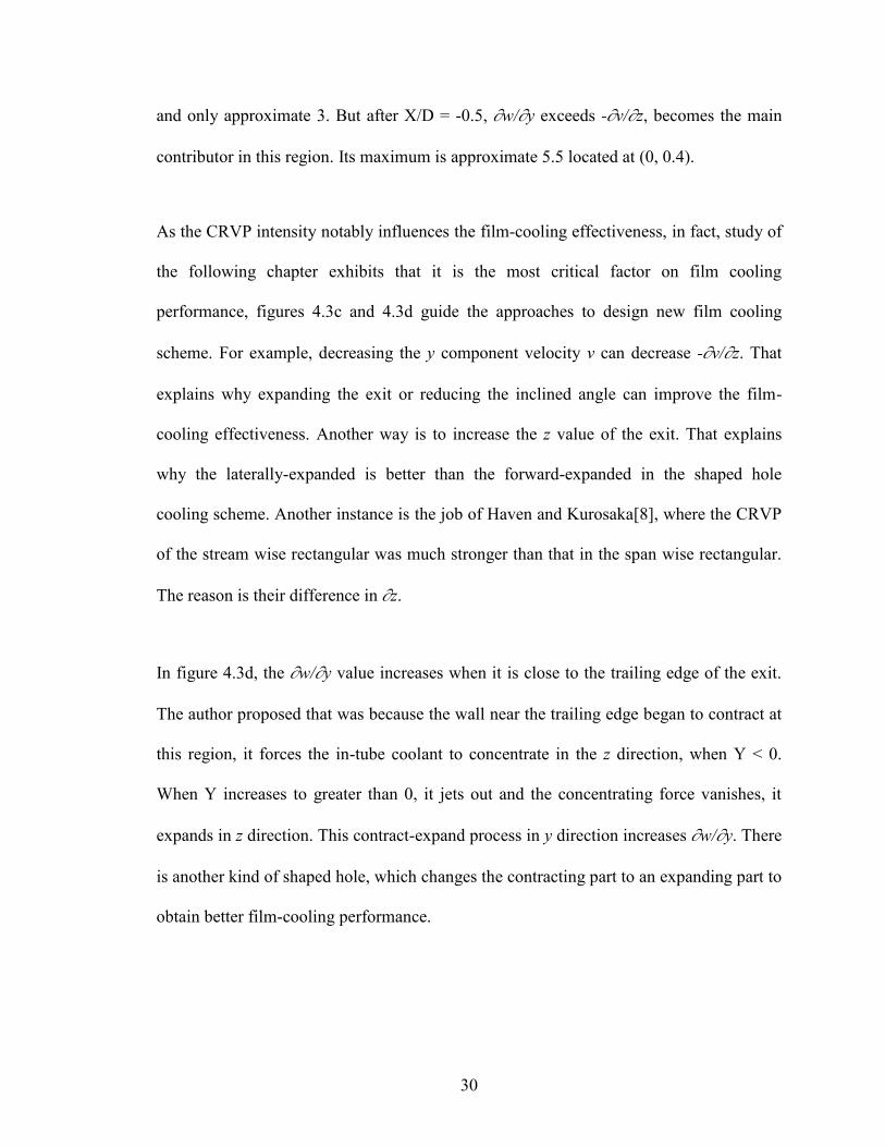
Contours of case 1’s vorticity and its contributors were pictured in figure 4.3 at a

horizontal plane Y/D=0.1. The edge of the hole exit was drawn as a semi ellipse on the

background. Figure 4.3a presents the distribution. Where the peak field is mainly in the

region above the exit, particularly along the exit edge, where is the jet/mainstream

interface. The maximum is about 15, at (-0.9, 0.5). Figure 4.3b is the x contour,

comparing with figure 4.3a, they have identical distributions. In fact, its maximum is

about 14.7, at the same location as that in the contour. Because:

When:

So:

The comparison of figures 4.3a and 4.3b illustrates that x is the main component of the

vorticity. And the other two components can be neglected.

From eq. (3.32), the terms of -v/z and w/y contribute to x and hence . Which were

presented in figures 4.3c and 4.3d. -v/z was found as the main contributor and its

maximum is approximate 11.6 located at (-0.9, 0.5), where w/y is much less than -v/z

30

and only approximate 3. But after X/D = -0.5, w/y exceeds -v/z, becomes the main

contributor in this region. Its maximum is approximate 5.5 located at (0, 0.4).

As the CRVP intensity notably influences the film-cooling effectiveness, in fact, study of

the following chapter exhibits that it is the most critical factor on film cooling

performance, figures 4.3c and 4.3d guide the approaches to design new film cooling

scheme. For example, decreasing the y component velocity v can decrease -v/z. That

explains why expanding the exit or reducing the inclined angle can improve the film-

cooling effectiveness. Another way is to increase the z value of the exit. That explains

why the laterally-expanded is better than the forward-expanded in the shaped hole

cooling scheme. Another instance is the job of Haven and Kurosaka[8], where the CRVP

of the stream wise rectangular was much stronger than that in the span wise rectangular.

The reason is their difference in z.

In figure 4.3d, the w/y value increases when it is close to the trailing edge of the exit.

The author proposed that was because the wall near the trailing edge began to contract at

this region, it forces the in-tube coolant to concentrate in the z direction, when Y < 0.

When Y increases to greater than 0, it jets out and the concentrating force vanishes, it

expands in z direction. This contract-expand process in y direction increases w/y. There

is another kind of shaped hole, which changes the contracting part to an expanding part to

obtain better film-cooling performance.

31

a) magnitude

b) x

c) -v/z

d) w/y

Figure 4.3 Contours of the baseline vorticity and its contributors above the exit (Y/D=

0.1, Br = 1).

32

Back to figure 4.1, in figures 4.1d and 4.1f, the contours of ωx were plotted overlapped

with streamlines. In the region above the exit, figure 4.1d for example, the positions of

the CRVP’s core and the ωx maximum are superposition. When moving to downstream,

these two positions branch progressively, but still very close in the near field, such as

figure 4.1f. According this observation, the vorticity and its contributors in the near field

of X/D = -1 to 5 were plotted in figure 4.4. In the whole range, ω and ωx are almost

coincidence. After X/D=0.7, they begin to divide very slowly. Their maxima, about 12,

are located close X/D= -1, then their values drop all the way. At X/D= 0, they are still

greater than 6.5. Then go down quickly to 2.2 at X/D= 0.7. Consequently, they decline

slowly to about 0.5 in the far field. The following two results are exhibited through the

distributions of ω and ωx:

The CRVP is mainly a pair of x direction vortices;

Figure 4.4 Vorticity and its contributors at CRVP’s core

0

3

6

9

12

15

-1 0 1 2 3 4 5

X/D

ω

ωx

-∂v/∂y

∂w/∂z

33

The CRVP mainly forms in the region above the exit, when it leaves the

exit, its vorticity drops quickly to a small value.

The -v/z in this figure has a similar trend to that of the vorticity. Its maximum is

located close X/D= -1, then it drops all the way. The curve of w/y is distinct from the

above, at first it creeps from X/D= -1 to close to X/D= 0, where it reaches its maximum,

about 4.2. Then it declines to the far field. As two terms of x, the curves of -v/z and

w/y demonstrate that, in the infancy of the CRVP’s formation, -v/z is its main

contributor. When the CRVP is developing above the exit, -v/z declines steeply and

w/y inclines, so the contribution of w/y becomes more and more. In the region

around the trailing edge, w/y converts into the main contributor, instead of -v/z.

Figure 4.5 2D streamlines comparison between the cases of FSIT and baseline at the Y-Z plane of

X/D = -0.25.

34

4.3 The effect of the in-tube boundary layer

The result of the FSIT case, which has a free slip in-tube wall, and its comparison with

the baseline are presented in this section. Figure 4.5 compares the CRVP at the Y-Z plane

of X/D = 0.25. The left part (Z/D < 0) is the streamlines of the FSIT case and the right

part (Z/D > 0) is those of the baseline. No distinction can be found here. The in-tube

boundary layer effect is found to be not necessary for the formation of CRVP, and it has

no distinct influence on the CRVP.

Figure 4.6 is the ωx contour of the FSIT case. Contrasting with figure 4.3b, the difference

can be neglected. However, the local maximum in this case is approximate 15, slightly

higher than that of baseline. The comparisons of the vorticity between the cases of FSIT

and baseline were shown in figure 4.7. With these quantitative comparisons, the minute

differences can be observed. Figure 4.7a shows the contrast of x at the CRVP cores. The

difference is clearer than the comparison of figures 4.3b and 4.6. The x of FSIT is

almost higher than that of the baseline in the whole range, except slightly smaller at the

region from X/D=0 to 1. This smaller x is a direct result of the differences in w/y in

this region, where the w/y of the baseline is slightly higher than of the FSIT, shown in

Figure 4.7b.

35

Figure 4.6 Contour of ωx above the exit in FSIT (Y/D = 0.1)

a) x at the CRVP cores b) -v/z and w/y at the CRVP cores

Figure 4.7 The comparisons of the FSIT case and the baseline.

0

5

10

15

-1 1 3 5 X/D

Baseline, ωx

Case FSIT, ωx

0

5

10

15

-1 1 3 5 X/D

Baseline, -∂v/∂z

Case FSIT, -∂v/∂z

Baseline, ∂w/∂y

Case FSIT, ∂w/∂y

36

These comparisons of the baseline and FSIT cases demonstrate that the in-tube boundary

layer has a minor reduction effect on the CRVP. This reduction results from the shear

layer’s velocity profile. The free slip boundary condition can sharpen the velocity profile.

It is worth to note that this result seems opposite to the conclusion in the job of Schlegel

et al. [17], where the boundary layer effect is found to strengthen the CRVP significantly

in JICF. The explanation is discussed in the following subsection.

4.4 The CRVP characters in film-cooling flow contrasting with those in

JICF

CRVP is a dominant vortical structure in both film-cooling flow and JICF. Plenty of

investigations were also performed in that in JICF. Even though the results obtained in

film cooling flow and JICF are usually compared to one another, their fundamental

mechanisms are not identical.

The CRVPs in both film-cooling flow and JICF are along the trajectory of the jet. Their

main components are different. In film-cooling flow, it is x, whereas y in JICF. That

results from their respective contributors. As it is described above, the main contributor

to the CRVP in film-cooling flow is -v/z. In contrast that in JICF, is supposed to be

u/z. This should be the reason behind the opposite effects of the boundary layer on the

CRVP. In film-cooling flow, the y-component velocity v in jet is higher than that in

mainstream. A sharp velocity profile in the in-tube boundary layer can raise the velocity

gradient of the shear layer. On the other hand, in JICF, the x-component velocity u in jet

37

is lower than that in mainstream. A sharp velocity profile will reduce the velocity

gradient.

This fundamental difference leads to other flow characters governing CRVP besides the

boundary layer effect. For example, it is supposed that the CRVP intensity in JICF would

not decay steeply even far away from the exit, contrasting to the falling down after

X/D=0 in film-cooling flow. Such behaviors are not the emphasis of present investigation

and will not be expended here.

38

Chapter 5

The Effects of Counter-Rotating Vortex Pair

Intensity on Film-Cooling Effectiveness

The simulation results of the 1 and 3 to 16 cases were presented and discussed in this

section in the following sequence. First, the effect of the nozzle scheme on the CRVP

intensity was presented followed by their film cooling performance. Then the effect of

the CRVP intensity was demonstrated. Finally, the effect of momentum flux ratio on the

film cooling effectiveness was exhibited.

5.1 The Effect of Nozzle Scheme on CRVP

The mechanism of the CRVP’s formation, which was shown in the above chapter, guides

an approach of decreasing CRVP intensity. According this mechanism, the CRVP

intensity can be decreased by decreasing two velocity gradients -v/z and w/y. Which

was applied in the nozzle scheme. Configuration A1 is comprised of a couple of orifice

plates on the cooling hole’s span-wise sides, shown as figure 1a. This design was

intended to increase the z in -v/z. This vorticity contours of this configuration and the

contributors were presented in figure 5.1, where the maxima are about 7, 6, 6 and 3.6 for

, x, -v/z and w/y respectively. In contrast to the baseline in figure 4.3, this

configuration decreases the CRVP intensity to about a half, mainly by decreasing the -

v/z. Another design, configuration A2, comprises a U-shape orifice plate. The plate’s

two parts on the span-wise sides were intended to decrease the -v/z term and the part

near the trailing edge was aimed to decrease the w/y term. The result of this

39

configuration was presented in figure 5.2, where the maxima are about 7.3, 6.8, 5 and 2

for, x, -v/z and w/y respectively. The values at (-0.9, 0.5), where the peak field of

the baseline located, is reduced. At (0, 0.4), where the baseline’s maximum of w/y

located, the vorticity is close to 0. This design seems to have reached the target of

reducing both -v/z and w/y. However, another peak field for these variables occurred

in the region of X/D > -1 and Z/D < 0.2, which enhances the CRVP intensity. The

simulation results of the configuration A3 were shown in figure 5.3, where the maxima

are 20, 18, 12 and 8 for , x, -v/z and w/y respectively. This configuration increases

the CRVP intensity.

The CRVPs of the four geometries at blowing ratio 1 were visualized in Figure 5.4 with

2D streamlines on the Y-Z plane of X/D = -0.25. As only half of a cooling hole is in the

computed domain, the data on the right side was mirrored to the left side for each

configuration. The CRVP intensity of configuration A1, in figure 5.4b, is the weakest,

while that of configuration A3, in figure 5.4d, is the strongest. The intensities of baseline

and configuration A2 are between those of the configurations A1 and A3, and the

intensity of baseline is stronger than that of the configuration A2. Their difference,

however, is not as great as that between configurations A1 and A3. In fact, table 3.1

demonstrates that the values of the baseline are higher than those of the configuration

A2 at the blowing ratios of 1, 1.5 and 2. But at the blowing ratio of 0.5, configuration A2

is slightly higher than baseline. The reduction of configuration A2 on the CRVP intensity

is shown more apparent when the blowing ratio increases.

40

a)

b) x

c) -v/z

d) w/y

Figure 5.1 Contours of the A1 vorticity and its contributors above the exit (Y/D= 0.1,

Br = 1).

41

a)

b) x

c) -v/z

d) w/y


Br = 1).

42

a)

b) x

c) -v/z

d) w/y


Br = 1).

43

The results shown in this subsection illustrate that the nozzle scheme control the CRVP

intensity by changing the velocity distribution on the hole exit. Configurations A1 and A2

decrease the CRVP intensity, and the decrease effect of configuration A1 is more notable.

The configuration A3 increases the CRVP intensity. The CRVP intensity at a specific

blowing ratio has the following sequence: configuration A1 < configuration A2 <

baseline < configuration A3, except for configuration A2 and baseline at blowing ratio

0.5.

5.2 The Film-Cooling Effectiveness of the Nozzle Schemes and the Effect

of CRVP Intensity

The film-cooling effectiveness for each blowing ratio was presented in Figures 5.5 and

5.6, for the centerline effectiveness and the span-wise average effectiveness respectively.

At the blowing ratio of 0.5, in figure 5.5a, the effectiveness curves are close, though

configuration A1 provides the best effectiveness, and avoids liftoff. Although

configuration A2 slightly outperforms the baseline somewhere close the hole, farther

away the trend is reversed. The performance of configuration A3 is the lowest. Figure

5.6a shows the similar results for the span-wise average effectiveness; configuration A1

performs the best and the configuration A3 has the lowest performance. Configuration

A2 is better where close the hole and the baseline shows better effectiveness when X/D >

2. The performance sequence in terms of effectiveness under this blowing ratio is:

configuration A1 > baseline configuration A2 > configuration A3. In fact, the film

cooling performance of the baseline is slightly better than that of the configuration A2

when compared further in figure 5.7a. And the CRVP intensity of the baseline is lower

than that of the configuration A2, unlike the results obtained at other blowing ratios.

44

a) Baseline b) A1

c) A2 d) A3

Figure 5.4 CRVP visualized on Y-Z plane with 2D streamlines (X/D = -0.25, Br = 1).

45

a) Br = 0.5 b) Br = 1

c) Br = 1.5 d) Br = 2

Figure 5.5 Centreline film-cooling effectiveness

0

0.2

0.4

0.6

0.8

1

0 10 20 30 40

Ce

nte

rlin

e e

ffe

ctiv

en

ess

X/D

Conf. A1, Average Vorticity = 0.124


Baseline, Average Vorticity = 0.331


0

0.2

0.4

0.6

0.8

1

0 10 20 30 40

Ce

nte

rlin

e e

ffe

ctiv

en

ess

X/D





0

0.2

0.4

0.6

0.8

1

0 10 20 30 40

Ce

nte

rlin

e e

ffe

ctiv

en

ess

X/D





0

0.2

0.4

0.6

0.8

1

0 10 20 30 40

Ce

nte

rlin

e e

ffe

ctiv

en

ess

X/D





46

a) Br = 0.5 b) Br = 1

c) Br = 1.5 d) Br = 2

Figure 5.6 Span-wise average film-cooling effectiveness

0

0.1

0.2

0.3

0.4

0.5

0 5 10 15

Span

wis

e a

vera

ge e

ffe

ctiv

en

ess

X/D





0

0.1

0.2

0.3

0.4

0.5

0 5 10 15

Span

wis

e a

vera

ge e

ffe

ctiv

en

ess

X/D





0

0.1

0.2

0.3

0.4

0.5

0 5 10 15

Span

wis

e a

vera

ge e

ffe

ctiv

en

ess

X/D





0

0.1

0.2

0.3

0.4

0.5

0 5 10 15

Span

wis

e a

vera

ge e

ffe

ctiv

en

ess

X/D





47

a) Include all data

b) Exclude the complete detached data

Figure 5.7 CRVP intensity effect on film-cooling effectiveness

0.00

0.05

0.10

0.15

0.20

0.25

0.30

0.35

0.0 1.0 2.0 3.0 4.0 5.0 6.0 7.0

Are

a A

vera

ge E

ffec

tive

ne

ss

Volume average X-vorticity

Br=0.5

Br = 1

Br=1.5

Br=2

y = -0.16x + 0.30 R² = 0.86

0.00

0.05

0.10

0.15

0.20

0.25

0.30

0.35

0.0 0.5 1.0 1.5

Are

a A

vera

ge E

ffec

tive

nes

s

Volume average X-vorticity

48

At a blowing ratio of 1, distinct performances were shown in figures 5.5b and 5.6b. The

film cooling effectiveness of configuration A1 is two times that of the baseline.

Configuration A3 is complete detached and its effectiveness is close to 0. The sequence

in terms of the film cooling effectiveness is as follows: configuration A1 > configuration

A2 > baseline > configuration A3. The same sequence, which is the opposite sequence of

their CRVP intensity, was observed for the remaining blowing ratios in figures 5.5c, 5.5d,

5.6c and 5.6d. The adverse effect of the CRVP intensity on the film-cooling effectiveness

is illustrated.

To depict this adverse effect more clearly, the film-cooling effectiveness was evaluated

with the area average value

and the CRVP intensity was evaluated with volume

average value . Based on the figure 5.6, a range of X/D = 0 to 5 reflected the

characteristics of the film cooling effectiveness. This part of the test plate was extracted

as the characteristic area to calculate

, which was plotted against in Figure 5.7a.

The data points were grouped according their blowing ratios. All lines are monotone. The

lines of blowing ratios 0.5 and 1 are close to linear, as are the first three data points of the

blowing ratios 1.5 and 2. Recall that the nozzle scheme isolated the Iov, which is 0.125,

0.5, 1.125 and 2 at blowing ratios of 0.5, 1, 1.5 and 2, respectively. As the the

investigation of completely detached flow is not the objective of this paper, the flow of

was considered as completely detached and excluded. Results were plotted

again in figure 5.7b. A correlation of

and was presented as:

(5.1)

The CRVP intensity is a critical factor governing the film-cooling effectiveness.

49

5.3 The Momentum Flux Effect on Film-Cooling Effectiveness

As previously mentioned, Iov considers the velocity distribution to be uniform, and it has

been isolated in the present study. After taking the velocity distribution into account, I

was also investigated. The results on two planes were presented in Figure 5.8. Figure

5.8a shows Ῑ at the hole cross-section. The data was grouped with two criteria, the dashed

line was based on geometries and the solid line was based on blowing ratios. For the

dashed lines, an obvious tendency is observed for each line. Which indicates that, for a

specific geometry, Ῑ at the hole cross-section plane has an adverse effect on

. This

agrees very well with the literature. However, when considering a wider scope in this

figure, this conclusion is not valid any longer. When the blowing ratio is unity, for

instance, configuration A1 exhibits the highest effectiveness; even if its value is larger

than those of configuration A2 and the baseline. No clear correlation can be found. The

was presented against the Ῑ at the hole exit in figure 5.8b. A similar trend is observed

in figure 5.8a. Figure 5.8 indicates that at either the cross-section or the exit is not a key

parameter governing the film cooling effectiveness.

50

a) At the hole cross-section

b) At the hole Exit

Figure 5.8 Effect of the area-average momentum flux ratio on film cooling effectiveness

0.00

0.05

0.10

0.15

0.20

0.25

0.30

0.35

0.40

0.45

0.50

0.0 1.0 2.0 3.0 4.0 5.0

Are

a A

vera

ge E

ffec

tive

nes

s

ī at hole cross-section

Br = 0.5 Br = 1

Br = 1.5 Br = 2

Conf. A1 Conf. A2

Baseline Conf. A3

0.00

0.05

0.10

0.15

0.20

0.25

0.30

0.35

0.0 0.2 0.4 0.6 0.8 1.0 1.2 1.4 1.6 1.8

Are

a A

vera

ge E

ffec

tive

nes

s

ī at hole exit

Br = 0.5

Br = 1

Br = 1.5

Br = 2

51

Chapter 6

Conclusions and Future Directions

6.1 Conclusions

In this study, through visualizing on the formation process of the CRVP in a cylindrical

film-cooling flow with a numerical simulation performed with the RKE model; hence

further analyzed the mechanism. About the CRVP formation, it has been found that:

By comparing the near field vortical structure of the results from RKE

model and DES model, the same CRVP is observed, even the in-tube

vortices are different. The CRVP’s characteristics can be captured by the

RKE model.

By visualizing the formation process in the results of RKE model and DES

model, no relation between CRVP formation and the in-tube vortex has

been found. At the same time, by comparing CRVP in the baseline and the

FSIT, the boundary layer effect has been found not to be necessary for the

CRVP formation. Only the jet/mainstream shear layer effect is the essential

source of the CRVP’s formation.

By further analyzing CRVP vorticity and its contributors in the film-cooling

flow, it has been found that the CRVP is an x direction vortical structure.

Therefore, its main promoters are the velocity gradients -v/z and w/y.

And in the baseline case, which is an ordinary cylindrical hole, -v/z is the

main contributor. The understanding of this mechanism is a guideline for

creating new high performance film-cooling schemes.

52

The in-tube boundary layer has a small reduction effect on the CRVP.

The CRVP in film-cooling flow is a similar vortical structure to that in

JICF. However, they are supposed to have distinct fundamental

mechanisms. That leads to their respective flow characters.

Applying the CRVP mechanism, directly guided a method to rein the CRVP. That was to

decrease the -v/z and w/y. Through the successful application of this method, three

typical configurations of nozzle scheme have been designed to control the CRVP

intensity and isolate the Iov factor. Among them, configuration A1 has decreased the

CRVP intensity drastically, configuration A2 has reduced the CRVP intensity slightly

and configuration A3 has increased the CRVP intensity. In fact, when designing a new

film cooling scheme, cooling hole tubes is not necessary to maintain identical if the

investigation objective is not the momentum flux ratio.

At the time of controlling the CRVP intensity, the nozzle scheme has changed the film

cooling effectiveness. Configuration A1 has improved the performance drastically,

configuration A2 has done that slightly and configuration A3 has decreased the film

cooling effectiveness. The adverse effect of the CRVP intensity on film cooling

effectiveness was implied. As the Iov has been isolated for each blowing ratio, this

adverse effect was not related to the Iov.

The further analysis of the relation between film cooling effectiveness, momentum flux

ratio and CRVP intensity has exhibited that the CRVP intensity is the critical parameter

governing the film cooling performance. A correlation of the parameters, eq. (5.1), has

53

been proposed. The momentum flux ratio, either of Iov or was not a key factor on the

film cooling performance. The traditional thought, which states that the film cooling

effectiveness rests with the momentum flux ratio, has dominated for several decades,

leads the designers to expand the exit as large as possible when creating new film cooling

schemes. In fact, expanding the hole exit area randomly is not the optimal approach to

improve the film-cooling effectiveness. The most critical parameters are the two velocity

gradients, the -v/z and w/y.

6.2 Future Directions

Numerical simulation has many advantages, but eventually it needs experimental

measurement validation. In the present investigation, as the nozzle scheme is a

completely new scheme, support from experiment data would drastically improve the

trustworthiness.

As the objective of the nozzle scheme is to control CRVP intensity, rather than high

performance, the best performance design is not finally achieved. Even in configuration

“A1”, the maximum of -v/z and w/y are 6 and 4 respectively, approximate 50% and

80% of those in the baseline, respectively. In principle, CRVP intensity can be decreased

to 0, and reach the best performance.

Vast efforts have been devoted to advanced film cooling scheme research. As lacking of

guideline, or guiding by the previous thought of momentum flux, these designs were

54

inefficient. Applying the conclusions of the present investigation, we can efficiently

design new schemes with both high performance and productivity.

JICF is also a kind of fundamental flow. In the present thesis, some distinct characters of

the CRVP in JICF are proposed. Relevant study need to be performed.

55

Publications

Conference Papers

1. H. Ming Li, O. Hassan, and I. Hassan, The effects of counter-rotating vortex

pairs’ intensity on film-cooling Effectiveness, ASME, Proceedings of the ASME

IMECE, Energy and Water Scarcity, Denver, Colorado, USA, IMECE2011-

64400, 2011.

2. H. Ming Li, and I. Hassan, The Formation of Counter-Rotating Vortex Pair in

Film-Cooling Flow and its Mechanism, 4th

International Conference on "Heat and

mass transfer and hydrodynamics in swirling flows”, Moscow, Russia, 2011.

Journal Papers under Preparation

1. H. Ming Li and I. Hassan, The Effects of Counter-Rotating Vortex Pair Intensity

on Film-Cooling Effectiveness, will be submitted to the ASME Journal of Fluids

in December 2011.

2. H. Ming Li and I. Hassan, The Formation of Counter-Rotating Vortex Pair in

Film-Cooling Flow and its Mechanism, will be submitted to the ASME Journal of

Fluids in January 2012.

56

References

[1] J.R. Pietrzyk, D.F. Bogard, and M.E. Crawford, Hydrodynamic Measurements of

Jets in Crossflow for Gas Turbine Film Cooling Applications, J. Turbomachinery,

vol. 111, pp. 139-145, 1989.

[2] J.R. Pietrzyk, D.F. Bogard, and M.E. Crawford, Effect of Density Ratio on the

Hydrodynamics of Film Cooling, J. Turbomachinery, vol. 112, pp. 437-443, 1990.

[3] A.K. Sinha, D.G. Bogard, and M.E. Crawford, Film-Cooling Effectiveness

Downstream of a Single Row of Holes With Variable Density Ratio, Transactions of

the ASME, vol. 113, pp. 442-449, 1991.

[4] R. J. Goldstein, E.R.G. Eckert, and F. Burggraf, Effect of Hole Geometry and Density

on Three-Dimensional Film Cooling, Int. J. Heat Mass Transfer, vol. 17, pp. 595-607,

1974.

[5] Y. Yu, C.-H. Yen, T. I.-P. Shih, M. K. Chyu, and S. Gogineni, Film Cooling

Effectiveness and Heat Transfer Coefficient Distributions Around Diffusion Shaped

Holes, Journal of Heat Transfer, vol.124, pp. 820-827, 2002.

[6] Michael Gritsch, Will Colban, Heinz Schar, and Klaus Dobbeling, Effect of Hole

Geometry on the Thermal Performance of Fan-Shaped Film Cooling Holes, Journal

of Turbomachinery, vol. 127, pp. 718-725, 2005.

[7] T. F. Fric, and A. Roshko, Vortical Structure in the Wake of a Transverse Jet, J. Fluid

Mech., vol. 279, pp. 1-47, 1994.

57

[8] B. A. Haven, and M. Kurosaka, Kidney and Anti-Kidney Vortices in Crossflow Jets,

J. Fluid Mech., vol. 352, pp. 27-64, 1997.

[9] B. A. Haven, D. K. Yamagata, M. Kurosake, S. Yamawaki, and T. Maya, Anti-

kidney Pair of Vortices in Shaped Holes and Their Influence on Film Cooling

Effectiveness, ASME, 1997, Int. Gas Turbine & Aeroengine Congress & Exhibition,

Florida, USA, 97-GT-45, pp. 1-8, 1997.

[10] D.K. Walters, and J. H. Leylek, A Detailed Analysis of Film-Cooling Physics: Part I

– Streamwise Injection With Cylindrical Holes, Journal of Turbomachinery, vol. 122,

pp. 102-112, 2000.

[11] D. G. Hyams, and J. H. Leylek, A Detailed Analysis of Film-Cooling Physics: Part III

– Streamwise Injection With Shaped Holes, Journal of Turbomachinery, vol. 122, pp.

122-132, 2000.

[12] Kelso, R.M., T.T. Lim, and A.E. Perry, An experimental study of round jets in cross-

flow, Journal Fluid Mechanism, vol. 306, pp. 111-144, 1996.

[13] Yuan, Lester L., Robert L. Street, and joel H. Ferziger, Large-eddy simulations of a

round jet in crossflow, J. Fluid Mech., vol. 379, pp. 71-104, 1999.

[14] Guo, X., W. Schroder, and M. Meinke, Large-eddy simulations of film cooling flows,

Computers & Fluids, vol. 35, pp. 587-606, 2006.

[15] Recker, Elmar, Walter Bosschaerts, Rolf Wagemakers, Patrick Hendrick, Harald

Funke, and Sebastian Borner, Experimental study of a round jet in cross-flow at low

58

momentum ratio, 15th Int Symp on Applications of Laser Techniques to Fluid

Mechanics, Lisbon, Portugal, pp. 1-13. 2010.

[16] Youssef M. Marzouk and Ahmed F. Fhoniem, Vorticity Structure and Evolution in a

Transverse Jet, J. Fluid Mech, vol. 575, pp. 267-305, 2007.

[17] Schlegel, Fabrice, Daehyun Wee, Youssef M. Marzouk, and Ahmed F. Ghoniem,

Contributions of the Wall Boundary Layer to the Formation of the Counter-Rotating

Vortex Pair in Transverse Jets, J. Fluid Mech., vol. 676, pp. 1-30, 2011.

[18] Karsten Kusterer, Dieter Bohn, Takao Sugimoto, and Ryozo Tanaka, Double-Jet

Efection of Cooling Air for Improved Film Cooling, Journal of Turbomachinery, vol.

129, pp. 809-815, 2007.

[19] James D. Heidmann, and Srinath Ekkad, A Novel Anti-Vortex Turbine Film Cooling

Hole Concept, Proc. Of GT2007, ASME Turbo Expo 2007, Montreal, Canada,

GT2007-27528, pp. 487-496, 2007.

[20] Alok Dhungel, Yiping Lu, Wynn Phillips, Srinath V. Ekkad, and James Heidmann,

Film Cooling From a Row of Holes Supplemented With Antivortex Holes, Journal of

Turbomachinery, vol. 131, pp. 021007-1-021007-10, 2009.

[21] J. Ely Marc, and B. A. Jubran, A Numerical Evaluation on the Effect of Sister Holes

on Film Cooling Effectiveness and the Surrounding Flow Field, Heat Mass Transfer,

vol. 45, pp. 1435-1446, 2009.

59

[22] J. Ely Marc, B. A. Jubran, A Numerical Study on Improving Large Angle Film

Cooling Performance Through the Use of Sister Holes, Numerical Heat Transfer, vol.

55, pp. 634-653, 2009.

[23] X. Z. Zhang, and I. Hassan, Film Cooling Effectiveness of an Advanced-Louver

Cooling Scheme for Gas Turbines, Journal of Thermophysics and Heat Transfer, Vol.

20, no. 4, pp. 754-763, 2006.

[24] Sung In Kim and Ibrahim Hassan, Unsteady Simulations of a Film Cooling Flow

from an Inclined Cylindrical Jet, Journal of Thermophysics and Heat Transfer, Vol.

24, no. 1, pp. 145-156, 2010.

[25] ANSYS FLUENT 12.0 Theory Guide, ANSYS, Inc., 2009.

the counter-rotating vortex pair in film-cooling …...the counter-rotating vortex pair in...

Documents