Generation and driving forces of plate-like motion and asymmetric subduction in dynamical models of an integrated

mantle-lithosphere system

Tomoeki Nakakuki*

Chiho Hamada

Michio Tagawa

Department of Earth and Planetary Systems Science

Hiroshima University

1-3-1 Kagamiyama, Higashi-Hiroshima, 739-8526, JAPAN

accepted for publication in Physics of Earth and Planetary Interiors,

Dec. 4, 2007.

*Corresponding author

Tel: +81-82-424-6579

Fax: +81-82-424-6579

E-mail: nakakuki@hiroshima-u.ac.jp

Abstract

The dynamical effects of an asymmetric subduction structure on the generation

of plate-like motion were investigated using two-dimensional numerical

models of the integrated lithosphere-mantle system. To dynamically generate

the plate boundary, we introduce a history-dependent rheology in which the

yield strength is determined by past fractures. Only the buoyancy due to the

internal density contrast consistently drives convective flow, including the

motion of the viscous lithosphere, without imposed boundary conditions. We

first investigate the effects of plate yield strength, friction at the plate boundary,

and plate age on the emergence of plate-like motion with asymmetric

subduction. Plate-like motion is generated when maximum plate strength is as

high as that estimated by experimental rheology studies. The reason for this is

that asymmetric subduction requires a plate-bending force much less than that

for symmetric subduction because the plate gently bends when one-sided

subduction occurs. In contrast, the strength of the plate boundary has to be

very small for emergence of subduction, as several previous studies on the

numerical convection and subduction modeling have pointed out. Development

of the subducted slab is also controlled by the age of the plate. In the early

stages of subduction, older plates increase their velocities faster because of

their larger negative buoyancy. After the slab develops, the plate stiffness, that

is, both the yield strength and the plate thickness, control plate velocity so that

an older plate subducts more sluggishly. We next explore effects of viscosity

layering in the underlying mantle, focusing on the mechanism in which the

asthenosphere promotes plate motion. The low viscosity under the lithosphere

enhances a mantle drag force that drives the plate, not only concentrating the

convective flow beneath the plate but also enlarging its aspect ratio. We also

examine longevity of the plate-like motion using the convection models with

asymmetric subduction. The asymmetrically structured subduction process

continues stably at high yield strength, at which episodic resurfacing or the

stagnant-lid mode occurs in the previous convection simulation studies. The

asymmetric subduction structure therefore has key roles in generating

plate-like motion as well as reducing the strength at the plate boundary.

Keywords

plate-like motion, mantle convection, asymmetric subduction, yield strength

1

1. Introduction 1

2

Understanding mechanisms that generate plate tectonics on the Earth is a 3

fundamental issue of geodynamics. The construction of a dynamic 4

mantle-convection model that includes plate tectonics is essential for directly 5

solving this problem. Difficulty in developing numerical models arises from the 6

complex rheology that causes lithosphere deformation in narrow regions such as 7

faults. In the last decade, progress in both computer hardware and software has 8

enabled us to incorporate more complex rheologies into high-resolution 9

numerical models (reviewed by Tackley, 2000a; Bercovici, 2003). 10

The rheology with yielding as the continuum limit of fracture was 11

introduced by Cserepes (1982) to produce plate-like behavior of the viscous lid. 12

Weakening due to the yield stress induces focused deformation in the viscous lid 13

and its plate-like movement. Plate-like motion is also produced in 3-D 14

convection systems (Trompert and Hansen, 1998). The instantaneous yielding 15

rheology, however, results in unstable behavior of the surface plate. Moresi and 16

Solomatov (1998) and Tackley (2000b) systematically investigate the range of 17

yield stress that generates stable plate motion using 2-D and 3-D models. They 18

show that the yield strength should be much smaller than that estimated from 19

experimental study (e.g., Kohlstedt et al., 1995) or from lithosphere deformation 20

(Cloetingh and Wortel, 1986; Gerbault, 2000) to produce stable, plate-like 21

motion. Tackley (2000c) and Richards et al. (2001) show that low 22

asthenospheric viscosity improves plate motion stability, although the yield 23

stress range is still far from experimental and observational study results. 24

Tackley (2000c) introduces the damage rheology proposed by Bercovici (1996, 25

1998) into his 3-D models. He finds that the damage rheology does not improve 26

the parameter range for generating plate-like motion. Ogawa (2003) surveys the 27

broad range of damage rheology parameters using 2-D models. He concludes 28

that the strength contrast between “intact” and “damaged” materials is important 29

for generating satisfactorily rigid plate-like motion. Auth et al. (2003) have 30

2

performed high-resolution mantle convection simulations with the damage 1

rheology to analyze the detailed damage rheology physics. They point out that 2

advection of damage in the plate interior broadens deformation and depresses the 3

stability of plate-like motion. Yoshida and Ogawa (2004) report the effects of 4

uprising plumes on the emergence of new plate boundaries. 5

Convergent plate boundaries, reproduced by mantle convection models 6

containing uniform rheology functions both with and without history 7

dependence are still not realistic because the subduction structure produced is not 8

one-sided, but two-sided. Davies (1989) imposes a dipped low-viscosity zone 9

on the convection model with a temperature-dependent viscosity to simulate 10

concentrated deformation at the plate boundary. In his model, plate-like motion is 11

produced with asymmetric subduction of the viscous layer. Lenardic and Kaula 12

(1994) show that the stagnant lithosphere becomes mobile when a low-viscosity 13

layer is introduced at the top of the viscous lid, although they use convection 14

models with a symmetric descending flow. Gurnis and his colleagues 15

incorporate a weak fault acting as the plate boundary into mantle convection 16

models (Zhong and Gurnis, 1995a, 1995b, 1996; Zhong et al., 1998; Gurnis et 17

al., 2000). In their model, a one-sided subduction structure is also generated, and 18

they point out that fault weakness is necessary to generate subduction. Honda et 19

al. (2000) propose introducing a moving layer with yielding as an expression of 20

history-dependent rheology to simulate a lubricating layer at the plate boundary, 21

and they show the possibility of an asymmetric structure’s emergence. The 22

moving layer with yield stress is also employed in the models developed by 23

Lenardic et al. (2000) and Moresi et al. (2002). These results imply that an 24

advection effect of localized weakness caused by the heterogeneous rheology 25

function is important to continuously generate asymmetric subduction with 26

decoupled plate boundaries. 27

We believe that an Earth-like asymmetric subduction style has a key role 28

in solving the discrepancy between the lithospheric strength of numerical models 29

and rheology experiments. The reason why we expect this is that flexure of the 30

3

plate at trenches is not intense, but moderate in the case of one-sided subduction. 1

Conrad and Hager (1999) and Schellart (2004) use kinematic numerical 2

modelings and analog experiments to show that plate bending at a trench is an 3

important resistance against plate motion. On the contrary, two-sided vertical 4

subduction needs sudden buckling at the convergent zone to generate excessive 5

lithospheric fracture. We therefore reexamine rheological parameter effects on 6

determining lithospheric strength using dynamical models that reproduce 7

one-sided subduction. For this purpose, we have developed numerical models of 8

the lithosphere-mantle system in which asymmetric subduction occurs, 9

introducing history-dependent yielding without imposed velocity boundary 10

conditions. In our model, we observe the evolution of lithosphere deformation 11

from initiation of subduction at the passive continental margin, with or without a 12

preexisting weak zone, to the succeeding development of the subducted slab and 13

plate motion. 14

First, we systematically investigate the effects of three variable 15

parameters that determine plate strength—yield strength of the brittle-ductile 16

transition layer in a lithosphere, the friction coefficient of the lithospheric brittle 17

layer, and the friction coefficient of a fault zone at the plate boundary—on the 18

emergence of subduction. We also consider effects of a preexisting weak zone 19

on subduction generation for various plate strengths. Second, lithosphere age in 20

the initial conditions is varied to examine lithosphere thickness effects. Third, 21

forces acting on the plate are quantitatively analyzed to understand the dynamical 22

mechanisms driving plate-like motion. The values of the driving forces obtained 23

will be compared with a torque balance analysis (Forsyth and Uyeda, 1975). 24

Fourth, the effects of viscosity layering are examined, especially focusing on the 25

low-viscosity asthenosphere beneath the plate. Here, we vary temperature and 26

pressure dependence of the viscosity to change the viscosity layering in the 27

underlying mantle. We investigate the interaction of the plate with the underlying 28

mantle, analyzing viscous coupling at the bottom of the lithosphere. Fifth, our 29

models are integrated over a long time period to examine plate subduction 30

4

longevity and the plate motion evolution. We focus on the time-dependent 1

behavior of the subducted slab and on the plate motion driven by the slab’s 2

negative buoyancy. 3

4

5

6

5

2. Model settings and basic equations 1

2

2.1 Model configuration 3

Figure 1 shows a schematic view of the model configuration. Here, we 4

use a 2-D model with Cartesian geometry to minimize numerical difficulties, to 5

handle a complicated rheology, and to perform high-resolution calculations. 6

Physical parameters are described in Table I, and the model settings are found in 7

Table II. In most cases, computations are performed to simulate the situation 8

until the slab reaches 300 to 400 km, except in the long-term models. The time 9

integration is less than 50 Myr, which is short enough to neglect internal heating. 10

For the long time-integration model (Runs 100L and 102L, Table II), we also set 11

the internal heating at zero because of the reason described in Section 3.5. In 12

most cases, we set the height h of the model to be 1320 km (twice the upper 13

mantle thickness), or 1500 km in the long time-integration. We use these values, 14

which are less than or about half the mantle thickness, to maximize the model 15

resolution. In the resolution-testing models, the height h is set at 660 km. The 16

horizontal length l is changed depending on the age of the oceanic plate in the 17

initial conditions (Table I), that is, a wider box is employed for models with 18

older oceanic plates. 19

We consider subduction of the oceanic lithosphere beginning at a passive 20

continental margin with or without a preexisting weak zone (Fig. 1). The models 21

presented here therefore consist of two regions — “oceanic” and “continental.” 22

The “oceanic” region has an oceanic lithosphere and underlying mantle. The 23

oceanic lithosphere is a surface layer with the same composition as that of the 24

underlying mantle and a high viscosity due to its low temperature. The 25

“continental” region consists of a continental lithosphere and underlying mantle. 26

The continental lithosphere includes an intrinsically buoyant layer simulating a 27

continental crust 35 km thick and a low-temperature mantle lithosphere beneath 28

the crust. Because we consider a simulated margin at an immobile continent, the 29

continental lithosphere is fixed at the right-side boundary (This effect will be 30

6

discussed briefly in section 4). The underlying mantle is identical to that of the 1

oceanic region. In two cases (Runs 50-12 and 13, Table II), the buoyant crust is 2

excluded. Namely, an overriding oceanic plate is also considered. 3

In our models, no external forces are imposed so that the driving forces 4

of the system are generated internally by density anomalies. Subduction, 5

however, is difficult to get started, and so we made the following assumptions. 6

(1) A plume that provides a positive mantle drag force exists. (2) The initial 7

temperature that produces a ridge-push force is set in the oceanic lithosphere. (3) 8

The basalt-eclogite transition is neglected. (3) The power-law dislocation creep is 9

parameterized as a low-viscosity channel. (4) The buoyancy of the basaltic layer 10

in the subducting lithosphere is neglected. (5) A weak zone is introduced into 11

most of the calculated models to produce a plate boundary in the initial 12

conditions. These will be discussed in Section 4. 13

The temperature of the oceanic lithosphere in the initial conditions (Fig. 14

1a) is determined according to the half-space cooling model with 20, 50 and 100 15

Ma. The temperature of the continental lithosphere in the initial conditions is set 16

to be horizontally uniform and the same as that of the oldest oceanic lithosphere. 17

In the underlying mantle, the initial temperature Ti is set to be adiabatic and 18

laterally homogeneous, namely, 19

20

Ti z( ) = TM + T0( )expαgz

Cp

⎛

⎝⎜⎞

⎠⎟− T0 , (1) 21

22

where TM is the mantle potential temperature (Celsius degree), T0 is the absolute 23

temperature of 0 °C, α is a thermal expansion coefficient, g is gravitational 24

acceleration, and Cp is specific heat. We impose a hot thermal anomaly with 25

dimensions of 50 400 km at the bottom-left corner to generate an upwelling 26

plume that creates a mantle drag force on the bottom of the plate (Fig. 1) for the 27

entire time. In this region, the potential temperature is set to be 200 K higher than 28

7

that of the surrounding mantle. This is a typical value of hot plume thermal 1

anomalies (McKenzie and Bickle, 1988). In the long time-integration, the lower 2

third of the model (1000 to 1500 km depth) has a fixed temperature provided by 3

Eq. (1) because of a reason discussed in Section 3.5. In this case, the plume 4

source with dimensions of 50 500 km is settled in the heat bath layer. 5

Mechanical boundary conditions for all the boundaries are set to be 6

tangential-stress-free to satisfy the condition of having no external forces except 7

buoyancy. The top boundary is set at a constant temperature T0, and the bottom 8

boundary is set at zero heat flux. Impermeable and insulated conditions are 9

applied to both side boundaries. 10

11

2.2 Rheology model 12

We use a viscous fluid model to approximate the mantle flow. The 13

rheology is expressed as a viscosity depending on temperature, pressure (depth), 14

stress and yielding history. The viscosity at zero stress (η0) is given by an 15

Arrhenius-type equation as 16

17

η0 = min AexpE * + pV *

R T + T0( )⎡

⎣⎢

⎤

⎦⎥,ηL

⎡

⎣⎢⎢

⎤

⎦⎥⎥

, (2) 18

19

where A is a pre-exponential factor, E* is activation energy, p is hydrostatic 20

pressure, V* is activation volume, R is a gas constant and T is temperature. The 21

symbol “min[a,b]” indicates a function to choose the smaller value of a and b. 22

Here, we introduce the viscosity limit ηL to keep the numerical calculation 23

accuracy. The estimated effective viscosity of the plate is on the order of 1024 to 24

1027 Pa from the lithosphere deformation study by Gordon (2000). We will 25

briefly discuss the effects of this viscosity truncation on subduction generation in 26

section 4. The values of E* and V* are based on those for olivine obtained by 27

Karato and Wu (1993). We use three combinations of E* and V* for the short 28

8

time-integration models and one combination for the long time-integration 1

models, as shown in Table II. Figure 2 shows the viscosity distribution with 2

depth at initial temperature conditions for short time-integration models. A is 3

fixed so that η0 is equal to the reference viscosity ηref = 5 1020 Pa (an average 4

of the observed viscosity values in the upper mantle, Milne et al., 1999; Okuno 5

and Nakada, 2001) at a depth of 410 km. The type I viscosity model (VM-I) has 6

constant values of E* and V* obtained for the diffusion creep of wet olivine. The 7

type II viscosity model (VM-II) has the same E* as that of the Type I rheology, 8

and V* decreases with depth and is smaller than that of Type I by 50 % at the 9

bottom of the model so that the viscosity becomes nearly constant beneath the 10

lithosphere. The type III viscosity model (VM-III) has two viscosity layers 11

divided at the depth of 410 km as shown in Fig. 2. In the upper layer, the values 12

of E* and V* are determined based on the dislocation creep of wet olivine. The 13

effect of the cubic power-law stress dependence is parameterized by reducing E* 14

and V* to half their values (Christensen, 1984). This introduces a weak 15

asthenosphere beneath the lithosphere because the larger value of V* introduces a 16

stronger pressure dependence than in VM-I. In the lower layer, the values of E* 17

and V* are set to be the same as those of VM-I. The pre-exponential factors for 18

the upper and lower layers are adjusted so that the viscosity values of both the 19

layers become identical to each other at the boundary (410 km depth). In the case 20

of the long time-integration model, we use a Type IIIa rheology (VM-IIIa) in 21

which V* decreases slightly with depth in the lower layer. 22

We introduce yield stress into the model to generate plate-like behavior in 23

the surface viscous layer. The effective viscosity η is determined by von Mises’ 24

criterion as 25

26

η = σY / 2ε II at σ II = σY (3) 27

η = η0 at σ II < σY , (4) 28

29

where σY is the yield stress as a function of the location, σ II and ε II are 30

9

second invariants of strain rate and viscous stress tensors defined by 1

2

ε II =1

2εij

2

i, j =1

2

∑ (5) 3

4

and 5

6

σ II =

1

2σ ij

2

i, j =1

2

∑ . (6) 7

8

9

Here, εij is the strain rate tensor defined by 10

11

εij =1

2

∂ui

∂x j

+∂u j

∂xi

⎛

⎝⎜⎞

⎠⎟, (7) 12

13

and the deviatoric stress tensor σ ij is linked to εij with constitutive relations 14

as 15

16

σ ij = 2ηεij . (8) 17

18

In most of the mantle except in a fault zone mentioned in the next paragraph, σY 19

simply depends on depth as 20

21

σY = min Y0 + cY ρ0gz,Ymax[ ] (9) 22

23

where Y0 is a cohesive strength, cY is a friction coefficient of the brittle layer 24

(Byerlee, 1978; Scholz, 1990) and Ymax is the maximum yield stress associated 25

with the brittle-ductile transition (BDT) of the lithosphere (Kohlstedt et al., 1995). 26

10

Thus, the model lithosphere consists of three layers as shown in Fig. 3. We 1

assume that Ymax is constant at depth, and treat it as a varying parameter in the 2

surface layers (Fig. 3). The value of Ymax changes from 200 MPa, which is the 3

stress level estimated from lithosphere deformation (Cloetingh and Wortel, 1986; 4

Gerbault, 2000), to 600 MPa, which is about 1.5 times higher than that estimated 5

from the experimental study (Kohlstedt et al., 1995). We also treat cY as a 6

parameter that is assumed to vary from 0.2 to 0.3. This value of cY is smaller than 7

the estimated value of 0.6 from an experimental rock fracture study (Byerlee, 8

1976) because weakening effects, such as hydration of the lithosphere, are 9

considered. We do not include yielding in the continental surface layer to 10

simulate stiff craton (Jordan, 1981), except in models without the continental 11

crust (the overriding plate is “oceanic” and has no buoyancy) or the long 12

time-integration models. 13

To introduce a “fault zone” for simulating the plate boundary, we 14

introduce a moving segment whose yield stress is determined by its past yielding 15

history. This simulates the segment whose mechanical strength is controlled by 16

pore pressure due to water content and fault gouges. Here, we call this a 17

“fault-zone segment.” The yield stress hysteresis in the fault zone segment is 18

shown in Fig. 4. The hysteresis of the yield stress is determined according to the 19

following rule: The yield stress in fresh material in the fault zone segment is 20

assumed to be the same as that of the normal lithosphere. Once yielding occurs 21

in the fault zone segment, the yield stress σY is reduced to a smaller value σF (Fig. 22

4), which is defined by 23

24

σ F = cFρ0gz , (10) 25

26

where cF is a friction coefficient of the “fractured” material. In order to indicate 27

the positions of the fault segment and the fractured material, we introduce a “fault 28

segment function” ΓF(x, z) and a “fractured segment function” ΓR (x, z). To settle 29

the location of the fault-zone segment at the surface of the plate, we formally 30

11

introduce the function ΓF. If the material becomes colder than a threshold 1

temperature, Th, we set a variable ΓF at 1. The value of Th is treated as a parameter 2

(Table 2) to test its effects. ΓF is advected independently of temperature by flow 3

according to a mass transport equation, 4

5

∂ΓF

∂t+ u ⋅∇ΓF = 0 (11) 6

7

When the stress reaches σY in the segment with ΓF = 1 (the fault-zone segment), 8

ΓR is set to be 1 (the fractured fault segment). The yield stress in the segment 9

with ΓR = 1 is set to be σF. ΓR is also transported by the flow according to Eq. (9). 10

We assume that recovery of the damage occurs at a depth of 330 km, and then ΓF 11

and ΓR are reset to zero. This depth must be deeper than about 150 km, which is 12

the depth of the deformed overriding plate edge. We also set a weak zone at the 13

top-left corner to simulate weakening by melting at mid-oceanic ridges. The yield 14

strength there is set to be σF. 15

16

2.3 Basic equations 17

We use an extended Boussinesq fluid to include the adiabatic 18

temperature influence on the viscosity layering in the model. The models 19

presented here are governed by an equation of motion that includes an equation 20

of continuity and a constitutive relation, an equation of state, an equation of 21

energy, and an equation of mass transport. We use dimensional forms of the 22

equations here because physical parameters are given by dimensional values due 23

to the model’s complexity. The equation of motion is expressed as 24

25

∂2

∂x2−

∂2

∂z2

⎛⎝⎜

⎞⎠⎟

η ∂2Ψ∂x2

−∂2Ψ∂z2

⎛⎝⎜

⎞⎠⎟

⎡

⎣⎢

⎤

⎦⎥ + 4

∂2

∂x∂zη ∂2Ψ

∂x∂z

⎛⎝⎜

⎞⎠⎟

= ∂ρ∂x

, (12) 26

27

where Ψ is a stream function defined by 28

12

1

u = u,w( ) =∂Ψ∂z

,−∂Ψ∂x

⎛⎝⎜

⎞⎠⎟ (13) 2

3

where (u, w) are x- and z-components of a velocity vector u. The vertical axis is 4

positive downward. An equation of state provides the density as 5

6

ρ = ρ0 1− αT( ) − ΔρcC (14) 7

8

where ρ0 is the mantle density at T = 0 °C, ρc is the density difference between 9

the mantle and the continental crust, and C is a composition function to express 10

the position of the continental crust (C = 1). C is governed by an equation of 11

mass transport: 12

13

∂C

∂t+ u ⋅∇C = 0 . (15) 14

15

The temperature is controlled by an energy equation including adiabatic heating 16

and viscous dissipation: 17

18

ρCp

∂T

∂t+ u ⋅∇T + u ⋅ ∇T( )s

⎡⎣⎢

⎤⎦⎥

= k∇2T + σ iji, j =1

2

∑ ∂ui

∂x j (16) 19

20

with 21

22

u ⋅ ∇T( )s= w

αg T + T0( )Cp

, (17) 23

24

where k is thermal conductivity. 25

We employ a finite difference method based on a control volume scheme 26

13

to solve the equations (Nakakuki et al., 1994). We adopt uniform square control 1

volumes of 5 km on each side for all the computations, except in one resolution 2

test case. The number of control volumes is changed according to the size of the 3

model, while the mesh size is fixed. The resolution test shows that the difference 4

between the plate velocities in the 5-km resolution model and the 2.5-km 5

resolution model is -2.8% after 2000 time steps and +2.5% after 4000 time steps. 6

The overall features of both the models are very similar. We therefore believe 7

that the 5-km grid has a sufficient resolution for the calculations presented in this 8

paper. A modified Cholesky decomposition method is applied to solve the 9

equation of motion (Eq. (12)). This makes the numerical solution stabilized 10

against sharp viscosity variations greater than 106. To avoid numerical diffusion 11

and phase errors of the mass transport equation (Eqs. (11) and (15)), a Cubic 12

Interpolated Pseudo-particle method (CIP method) is adopted (Takewaki et al., 13

1985). The CIP method is a highly valid method for solving problems with 14

sharp interfaces in computational fluid dynamics. Iwase and Honda (1992) 15

confirmed its validity for mantle convection calculations. A first-order Euler 16

method is applied to integrate the equation of energy (Eq. (16)) through time. 17

The size of time steps is changed so that the maximum value of the Courant 18

number ci, j 19

20

ci, j =ui, jδt

δ x+

wi, jδt

δz (14) 21

22

becomes equal to 0.1, where ui, j and wi, j are velocity components on the mesh, δt 23

is a time-step interval, and δx and δz are mesh sizes for the x and z directions, 24

respectively (but δx = δz because we use a uniform square grid). 25

26

14

3. Results 1

2

We systematically investigated the effects of plate yield strength, friction 3

at the plate boundary, plate age and viscosity layering in the underlying mantle 4

on the generation of plate-like motion. Our models have many physical 5

parameters because a complex rheology is required to reproduce the plate-like 6

behavior of the surface layer. We have performed 50 runs in total, including 2 7

runs for the resolution test as shown in Table II. All simulations were started 8

from conditions simulating a passive continental margin without a subducted 9

slab (Fig. 1a). Details of model settings and variable parameters will be 10

explained in the following sections. 11

12

3.1 Strength of the plate interior and the plate boundary 13

We first investigate influences of plate interior strength (cY, and Ymax), 14

friction of the plate boundary, (cF), and the style of the initial weak zone. We 15

examine the Series 50 models here, in which VM-I’s temperature- and 16

pressure-dependent viscosity (Fig. 2) is used and the initial plate age is set to be 17

50 Ma. Three types of initial weak zone are considered as illustrated in Fig. 5. 18

We place a segment with a history-dependent rheology at the ocean-continent 19

plate boundary in all the cases. The initial strength of the fault segment is 20

changed according to the initial conditions. Type-1 initial conditions (IC1, Fig. 21

5(a)) have a segment whose “fractured” yield strength is defined by Eq. (8). In 22

IC1, the “fractured” segment penetrates to the bottom of the thermal boundary 23

layer (depth of 150 km). In Type-2 initial conditions (IC2, Fig. 5(b)), the 24

fractured fault segment reaches to the bottom of the continental crust (depth of 35 25

km). In Type-3 initial conditions (IC3), the segment does not have “fractured” 26

strength so that the plate boundary has the same strength as that of ambient plate 27

materials in the initial conditions. 28

Figure 6 shows the evolution of the viscosity field and the surface 29

velocity for Run 50-01. This case has cY of 0.2, and Ymax of 200 MPa with IC1. 30

15

The oceanic (left) plate begins to subduct into the underlying mantle when the 1

ascending plume starts to interact with the oceanic plate (26 Myr). The forces 2

driving the plate will be discussed in Section 3.3. Asymmetric structure is first 3

produced due to the asymmetric (i.e., dipped) configuration of the initial weak 4

zone. The buoyancy of the continental crust is not always essential for initiating 5

subduction (Run 50-12 and 13). Compression and bending of the subducting 6

plate continuously generates damaged segments at the surface of the plate. This 7

damaged region is advected into the shear zone by the lithosphere’s motion. By 8

this mechanism, the history-dependent rheology continuously produces the fault 9

zone segment with weak strength at the plate boundary. The asymmetric 10

structure is therefore maintained during slab growth. Figure 7 shows a snapshot 11

of Run 50-01 in 46 Myr. The surface velocity (Fig. 7, top) and the stream lines 12

show that the strain in the subducting lithosphere is concentrated at the plate 13

boundary region and the internal segments of the high-viscosity layer very 14

slightly deform so that the surface layer behaves as a rigid plate. Most of the 15

lithosphere, except about 20 km near the ridge and 500 km near the trench, has a 16

strain rate (s-1) on the order of 10-18. Both plate-like behavior of the lithospheric 17

layer and one-sided subduction are produced. 18

We summarize the effects of initial conditions of cY and Ymax in the 19

diagram shown in Fig. 8. In these cases, cF is fixed at 0.01. In any case with IC1, 20

oceanic plate subduction can be initiated even when Ymax 400 MPa with cY of 21

0.3. This value is comparable to the fracture strength estimated by Kohlstedt et al. 22

(1995). The subduction structure is very similar when the viscosity-layering 23

model is identical. When the partial weak zone (IC2) is assumed in the initial 24

conditions, subduction of the plate is generated only in the case when Ymax = 100 25

MPa, and when Ymax = 200 and cY = 0.1 MPa. Introduction of stronger 26

convective flow to the underlying mantle (Run 52-21) or the asthenosphere (Run 27

52-22) enables generation of subduction at Ymax of 200 MPa and cY of 0.2 28

(shown by the diamond in Fig. 8). Either increasing or decreasing the plate age 29

does not affect subduction generation with IC2. The details are described in 30

16

Sections 3.2 and 3.4. In all the cases with IC3, subduction is not initiated. 1

We also examine the friction coefficient of the plate boundary (cF). Here 2

cY and Ymax are fixed at 0.2 and 200 MPa, respectively. Subduction is generated 3

only when cF = 0.01. Analysis of the driving/resisting forces of the plate shows 4

that friction at the plate boundary accounts for a considerable amount of 5

resistance against the plate motion (see Section 3.3). This value of cF is much 6

smaller value compared with Byerlee’s law (Byerlee, 1978) for rock fracture 7

(0.6). When cF is larger than 0.01, the resistance from the overriding plate is too 8

large for the driving force to generate subduction. 9

We test the threshold temperature of history-dependent rheology (Th), 10

that is, the effects of the fault segment thickness (run 50-08, 100-07 and 11

100L-03). The thickness systematically affects the plate velocity and the growth 12

of the subducted slab. The style of the velocity variation is very similar, but the 13

time elapsed to reach the same velocity is about 10 to 30 % longer. We can 14

therefore only discuss relative effects of the rheological parameters on the 15

evolution time and not absolute values. 16

17

3.2 Age of the oceanic plate and evolution of the plate motion 18

We next investigate effects of the oceanic plate age (AP). The age of the 19

plate in the initial conditions is set to be 20 Ma (Series 20), 50 Ma (Series 50), or 20

100 Ma (Series 100). The styles of the subducted slab are very similar in the 21

three different models because the dip angle of the slab is strongly constrained 22

by the initial weak zone. Figure 9 shows the evolution of the oceanic plate 23

velocity for six models with AP of 20, 50 and 100 Ma, Ymax of 200 and 600 MPa, 24

and cY of 0.2 and 0.3. 25

In the case of 20 Ma (the red lines, Fig. 9), plate motion does not grow 26

for 30 million years following inception but rapidly develops thereafter, because 27

negative buoyancy does not grow large enough for the plate to founder into the 28

mantle. The differences are very small in the early stages of evolution (t < 30 29

Myr). The evolution of plate motion is not affected by changing both cY and Ymax. 30

17

The reasons for this are that the brittle-ductile transition (BDT) layer does not 1

exist (Fig. 3) because of the plate thickness, and that only the brittle layer of the 2

plate causes a difference in plate strength. When the slab penetrates to a depth of 3

more than about 200 km, the velocity dependence on Ymax appears, because Ymax 4

has substantial strength effects on the subducted slab. 5

In the case of AP = 50 Ma (the blue lines, Fig. 9), subduction grows 6

faster than in the model with AP = 20 Ma because the lithosphere has a more 7

negative buoyancy. The internal plate strength (cY and Ymax) causes a larger 8

difference in the evolution of plate velocity than in the case with AP = 20 Ma. The 9

friction coefficient cY is a more important parameter for determining the evolution 10

of plate motion than Ymax because BDT layers (Fig. 3) occupy a significant 11

portion of the surface plate only when cY = 0.3. 12

In the case of AP = 100 Ma (the green lines, Fig. 9), the plate strength 13

causes the largest difference of the plate motion evolution among the calculated 14

models. In this case, Ymax differences affect the evolution of plate motion more 15

than in the other cases. Before about 25 Myr, subduction develops faster in the 16

cases with younger plates because older plates are heavier than younger plates, 17

so older plates have larger driving forces. In the later stages, the plate with Ap = 18

100 Ma subducts more sluggishly than cases with younger plates because the 19

thick plates have bending stiffness. 20

We also performed four calculations with IC2 (Run 20-21 at cY of 0.02 21

and Ymax of 200 MPa, Run 20-22 at cY of 0.02 and Ymax of 100 MPa, Run 100-21 22

at cY of 0.02 and Ymax of 200 MPa, and Run 100-22 at cY of 0.02 and Ymax of 100 23

MPa). The plate age does not affect the emergence of subduction because both 24

the ridge-push force and fracture strength for generating the plate boundary 25

increase proportionally with plate age. 26

27

3.3 Stress field and driving forces of the plate 28

We analyze stress fields and forces acting on the subducting plate to 29

understand the driving force of subduction. Figure 10 shows the stress fields of 30

18

Run 50-01 in which plate-like behavior is produced. We define the “lithosphere” 1

as a segment with temperature less than 1050 K or viscosity larger than 3 1021 2

Pa s, where the velocity is nearly constant. The boundary of the lithosphere is 3

indicated with green lines in Fig. 10. We observe that high stress regions are 4

settled in the lithosphere. This means that the plate propagates stress, or in other 5

words, the plate acts as a stress guide. The normal stress is horizontal 6

compression in most of the plate except in regions near a ridge or trench. The 7

compressional stress is generally observed when plate-like behavior is generated 8

in the surface. In this case, the tensional stress is produced in limited regions. 9

Plate spreading near the ridge causes the tension. The plate bends downwards in 10

the “outer rise” region near the trench so that tensional stress is induced in the 11

upper side of the plate. The horizontal strain rate averaged in the outer rise region 12

becomes negative, so that the plate is also compressed in this area. A wider 13

region with tensional stress is generated in the case of VM-III (see section 3.5). 14

The evolution of forces acting on the plate for Run 50-02 with plate 15

velocity and slab depth is shown in Fig. 11. We name the forces in Fig. 11b 16

according to Forsyth and Uyeda (1975). We describe the forces acting on the 17

plate by classifying them as driving forces (the solid lines, Fig. 11b) and 18

resisting forces (the dashed lines, Fig. 11b). The driving force is generated by 19

three sources, including pressure differences due to the shape of the plate 20

(ridge-push force, RP), viscous drag due to convective flow in the underlying 21

mantle (driving mantle-drag force, DF+), and negative buoyancy of the slab 22

(slab-pull force, SP). RP is calculated from the pressure difference between the 23

ridge and subdcution zone (Turcotte and Schubert, 1982), assuming that the 24

compensation depth is 150 km. We neglect topographic uplift caused by the 25

plume-ridge interaction because of the asthenosphere’s low viscosity. The 26

resisting force in the early stages of subduction consists of viscous stress from 27

the underlying mantle (resisting mantle-drag force DF-), friction at the plate 28

boundary (continental resistance, CR), and bending of the plate pushed by the 29

overriding plate (plate bending, PB). Because viscous resistance against the 30

19

subducted slab (slab resistance, SR) is not significant for subduction initiation, it 1

is not shown in Fig. 11b. The mantle-drag force (DF), which is the total viscous 2

stress between the plate and the underlying mantle (Forsyth and Uyeda, 1975), 3

acts as either an integrated driving or resisting force. DF is therefore separated 4

into two parts, namely, DF+ and DF-, which are the integrals of shear stress 5

dragging the plate in the moving and opposite directions. Plate bending (PB) is 6

the same as a slab suction force (Forsyth and Uyeda, 1975). 7

In the initial stage of subduction, RP and DF+ account for the plate 8

driving force. When a combination of RP and DF+ overcomes the resisting 9

forces (CR and PB), the plate begins to move in the direction of the trench and to 10

thrust under the overriding plate. RP increases with time because the plate 11

becomes thicker with cooling. DF+ has 1/2 of RP’s magnitude, but it has an 12

important role in initiating subduction by dragging the plate in the early stages of 13

subduction generation. Lack of DF+ force in a no-plume model (Run 50-11, 14

Table II) initiates no subduction. When the upwelling plume interacts with the 15

plate (near 30 Myr), DF+ increases and reaches an extremum (Fig. 11b). At the 16

same time, the plate velocity sharply increases, and a small plate velocity peak is 17

observed (Fig. 11a). CR and PB contribute a substantial portion of the force 18

resisting plate motion. In the early stages, the magnitude of CR is slightly larger 19

than that of PB. Although both CR and PB increase after 20 Myr, the increase of 20

PB is more pronounced. The accelerating plate velocity induces an increase in 21

plate yielding at the trench so that PB grows. The fault length is extended by 22

plate thickening due to cooling with time and by deformation of the overriding 23

plate entrained by the subducting plate. This causes CR to increase, as CR is 24

proportional to the square of the fault length. The increase in CR and PB causes 25

a momentary decrease in the plate velocity when the plate velocity is more than 2 26

cm yr-1. Although cF of 0.01 induces a significant resistive force in the magnitude 27

of CR, subduction can be generated. Increasing cF to 0.02 is enough to prevent 28

the plate from subducting, because CR is proportional to cF. SP increases as the 29

subducted slab is developed, and finally dominates after the slab penetrates to a 30

20

depth of 120 km (Figs. 11a, b). After this time, the plate velocity grows quickly. 1

DF- exceeds DF+ so that the mantle drag becomes resistive in total. 2

3

3.4 Viscosity layering and asthenosphere 4

We next consider effects of viscosity layering in the mantle, and we 5

especially focus on the roles of the low-viscosity asthenosphere. We employ two 6

types of viscosity structure (VM-II and VM-III, Fig. 2) other than the standard 7

model (VM-I), changing the activation energy E* and volume V*. 8

Figure 12 shows snapshots of Run 52-01’s viscosity field. In this case, 9

the lower mantle has low viscosity so that the ascending flow of the hot plume is 10

faster than that of the VM-I case in the lower mantle. We also assume a relatively 11

weak lithosphere (cY = 0.1). A vigorous convection current driven by the 12

upwelling plume induces a strong drag along the base of the lithosphere. In 13

addition, the convection current is concentrated in the left half of the model 14

because the underlying mantle has a nearly constant viscosity. The drag force 15

pushes a part of the plate only near the ridge. These cause broad deformation of 16

the lithosphere so that it does not behave like a rigid plate. If cY is assumed at 0.2, 17

plate-like motion is generated (Run 52-02). 18

In the case of VM-III (Run 52-03 to Run 52-05), when the viscosity has 19

a stronger pressure dependence in the upper layer of the mantle (Fig. 2), a 20

distinctive low-viscosity layer is formed beneath the lithosphere (Fig. 12). The 21

plate starts to move with greater velocity (4 cm yr-1) than those of VM-I cases 22

even before the upwelling plume directly contacts the bottom of the plate. The 23

convective flow induced by the upwelling plume broadens horizontally because 24

of the viscosity stratification (Fig. 12, bottom). This generates a drag force acting 25

uniformly on the base of the lithosphere, so that the drag on the plate works 26

more effectively in spite of the asthenosphere’s low viscosity. In this stage, a 27

tensional stress is observed around the 1000 km region near the trench. 28

Moreover, the smaller E* in VM-III causes a thinner mechanical plate than that 29

in VM-I. This causes a smaller bending resistance of the subducting plate. The 30

21

plate velocity therefore grows faster than that of Run 50-01 does. The plate 1

velocity of Run 52-03 reaches 12 cm yr-1 at its peak because the resistance from 2

the ambient mantle is at a minimum. The velocity variation is larger than that of 3

the VM-I rheology. The velocity of the plate is strongly changed by the viscosity 4

layering structure. 5

Figure 13 shows the horizontal velocities for Run 50-01 (VM-I) and 6

Run 52-03 (VM-III) at the centre of the model. The lines with solid symbols 7

show the velocity when the driving mantle drag force is more dominant than the 8

resisting force and the lines with open symbols show velocities in the opposite 9

condition. In the former condition, the velocity beneath the plate becomes faster 10

than that of the surface (plate) motion in Run 52-03. The asthenosphere 11

promotes horizontal flow beneath the lithosphere. As Fig. 12 shows, the 12

viscosity layering also causes the large aspect ratio of the underlying convective 13

flow. The model’s asthenosphere therefore enhances the driving force of the 14

plate. Figure 14 shows the mantle-drag forces (both DF+ and DF-) of Run 15

50-01 (VM-I) and 52-03 (VM-III). The magnitude of DF+ in Run 52-03 is as 16

large as that in Run 50-01 in spite of the 10-times-lower viscosity when DF+ 17

becomes larger than DF-. The plate velocity increase (up to 12 cm yr-1) in Run 18

52-03 induces the enlargement of DF- around 6 Myr. Because of the low 19

viscosity in the asthenosphere, DF- in Run 52-03 is smaller than in Run 50-01 20

although the former’s plate velocity is 3 times larger than that of the latter. 21

We also examine effects of viscosity layering on subduction generation 22

when the initial weak zone is absent (Runs 52-21 and 52-22). The values of Ymax 23

and cY are taken to be the same as those of Run 50-11, in which subduction 24

cannot occur. In Run 52-11, strong dragging by the mantle flow causes 25

subduction generation. In Run 52-12, subduction can be generated by the same 26

mechanisms that encourage fast growth of the plate velocity in Run 52-03. 27

28

3.5 Longevity of the subduction and evolution of the slab 29

In the last analysis, we examine subduction longevity and evolution of 30

22

the subducted slab. For this purpose, we execute the model as long as CPU time 1

permitted. Because each run takes about 500 hours of CPU time, we perform 4 2

runs with different asthenosphere settings (Runs 100L and 102L), “fault zone 3

segment” thicknesses (Run 102L-02), and lithospheric internal strengths (Run 4

102L-03). Because we are focusing on the plate and the upper mantle slab 5

dynamics, the temperature in the lower 500 km of the model is fixed to the 6

mantle adiabatic temperature to avoid having the slab stagnant above the bottom 7

of the model layer. The other important advantage is that the underlying mantle 8

temperature is constant in time. We can therefore remove the effects of 9

temperature-dependent viscosity variations to focus on stability and longevity of 10

the subducting slab. We use the VM-Ia (Run 100L-01) and VM-IIIa (Runs 11

102L-01 to 03) viscosity layering (Section 2.2) in which V* in the lower layer is 12

slightly reduced with depth (Table I) so that the velocity of the plate becomes 13

about 5 to 10 cm yr-1. In addition, the rheology of the overriding plate may affect 14

its stability. We therefore introduce yielding into the continental crust layer, and 15

set the E* and V* (Table I) in this layer to match those of granite (Kohlstedt et al., 16

1995). This, however, does not affect longevity of the plate motion. 17

Figure 15 shows snapshots of the viscosity field for Run 102L-02. The 18

subduction and plate-like motion of the surface layer continue to the end of the 19

calculations. In the cases with a low-viscosity asthenosphere (Runs 102L), the 20

deeply subducted slab swings because the high-viscosity deep mantle resists the 21

descending slab. When the subducted slab is convex (65 Myr in Fig. 15), the 22

plate moves slightly faster than when it is nearly vertical or concave (53 Myr). 23

Small-scale instabilites beneath the lithosphere occur with fluctuations of the 24

uprising flow (43 to 128 Myr). These quickly disappear after the uprising plume 25

becomes stationary. Afterwards, new instabilities are generated beneath the 26

lithosphere older than 60 Ma (148 Myr). The small-scale instabilities are not 27

observed in the case with a more viscous asthenosphere (100L-01). 28

The velocities of the subducting plate for Run 100L-01 through 102L-03 29

are shown in Fig. 16. In the case of Run 100L-01 without the low-viscosity 30

23

layer, the velocity converges to 4 - 5 cm yr-1. In Runs 102L-01 to 03 with the 1

low-viscosity asthenosphere, the velocities peak at 8 - 9 cm yr-1 when the slab is 2

sinking at a depth around 300 km. After that, the plate velocity finally converges 3

to 4 - 5 cm yr-1 in Runs 102L-01 and 02 and 3.5 - 4.5 cm yr-1 in Run 102L-03. 4

The low-viscosity asthenosphere, therefore, does not significantly influence the 5

plate motion after the subducted slab develops. The plate motion under the larger 6

yield stress condition (600 MPa, Run 102L-03) is slightly less than that under 7

the smaller yield stress condition (300 MPa, Run 102L-01). The thickness of the 8

“fault zone segment” does not affect the terminal plate motion velocity (Run 9

102L-02). Because resistance to the subducted slab is the largest of the resistive 10

forces, the mantle viscosity predominantly controls the descending velocity of 11

the developed slab. Fluctuation of the plate velocity after it reaches terminal 12

velocity is caused by slab deformation in the depth-dependent viscosity layering. 13

The slab is vertically compressed because the tip of the slab receives greater 14

viscous resistance than the shallower part does. 15

16

24

4. Discussion 1

2

We construct integrated numerical models of the plate-mantle system to 3

investigate effects of asymmetric subduction structures on the generation of 4

surface plate-like motion under various plate strengths and tectonic settings. In 5

our models, introducing a history-dependent yield strength is important for 6

generating an asymmetric subduction structure. Our proposed history- dependent 7

yield strength is similar to the limit of the damage rheology model (Auth et al., 8

2003), proposed first by Bercovici (1996), with extremely strong temperature 9

dependence, fast damage growth, and slow damage healing. The sharp 10

temperature dependence in the generation of fractures is able to produce 11

asymmetry because the position of the weak zone is limited to the plate surface. 12

In cases with gentler temperature dependence, symmetric subduction over a 13

broader plate boundary area would be produced. The advection of past fractures 14

preserves the damage and its asymmetric distribution, promoting consecutive 15

weak zones at the surface of the subducting plate. On the contrary, the damage 16

advection term is smaller than the source and healing terms in models with a 17

damage rheology (Ogawa, 2003; Auth et al., 2003). This may induce symmetric 18

subduction. 19

We first show that the emergence of plate-like motion with subduction is 20

insensitive to the brittle-ductile transition (BDT) strength of the plate interior, but 21

sensitive to friction on the plate boundary. If the plate boundary strength is small 22

enough, subduction occurs even at the highest BDT strength value (600 MPa). 23

Subduction generation does not strongly depend on the plate strength because 24

Earth-like asymmetric subduction needs a small degree of weakening for the 25

lithosphere to bend and allow the plate to drop into the mantle at the trench. 26

Yielding in the whole plate must occur to generate symmetric subduction. In this 27

case, the plate bending force (PB) has to be on the order of 1013 N m-1 with Ymax 28

= 200 MPa. The PB for asymmetric subduction (Fig. 11b) is much smaller than 29

that for symmetric subduction, although it is a significant resistive force. The 30

25

subducted slab can be formed when the friction coefficient (cF) of the fault zone 1

at the plate boundary is small ( 0.01). This value may be extraordinarily small, 2

so that excessive reduction of the plate boundary strength due to hydration at the 3

plate boundary (e.g., Jambon and Zimmermann, 1990) is therefore necessary to 4

generate subduction. Sensitivity to the plate boundary strength was predicted by 5

McKenzie (1977), and it is consistent with the conclusions of previous studies 6

(Toth and Gurnis, 1998; Conrad and Hager, 1999) focused on initiation of 7

asymmetric subduction. In our models, resistance at the plate boundary (CR) 8

accounts for the largest portion of resistive force in the early stages of 9

subduction. The friction coefficient cF corresponds to CR, which is the integral 10

of friction along the fault. When the plate thickness reaches the level attained at 11

100 Ma, the cF value of 0.005 coincides with the mean CR/RP ratio obtained by 12

torque-balance analysis (Forsyth and Uyeda, 1975). The friction coefficient 13

expected from observational studies should be even smaller than that employed 14

here. If that is true, the plate bending force (PB) is the largest of the resistive 15

forces. 16

When the initial conditions do not include the weak zone (IC3, Fig. 6), a 17

subducted plate cannot be generated under any conditions using the yield 18

strength in our models. To generate fault zones in the intact lithosphere, the 19

magnitude of the force must be on the order of 1013 N m-1, which is the integral 20

of the plate’s internal strength. Among the forces considered here, only the slab 21

pull (SP) can provide that level of force. Introduction of a partial initial weak 22

zone (IC2, Fig. 6) can initiate subduction when the yield strength is as small as 23

200 MPa (Fig. 8). With a larger maximum plate strength, an initial weak zone as 24

deep as the bottom of the lithosphere (IC1) is required to initiate subduction. 25

Mechanisms at least partially responsible for fracturing the plate, such as 26

sediment loading (Cloetingh et al., 1982; Branlund et al., 2001; Regenauer-Lieb 27

et al., 2001), plume intrusion (Turcotte et al., 1977; Kemp and Stevenson, 1996), 28

or transformation of past fracture zones (Gurnis et al., 2000), would be 29

important for generating new subduction when we introduce neither a weak zone 30

26

nor smaller plate strength. If subduction is initiated by these mechanisms, a drag 1

force (DF+) exerted by the underlying convective flow is also important to bend 2

the plate until the slab-pull force is enlarged. Hall et al. (2003) have succeeded in 3

spontaneously producing a developed subduction with backward slab motion 4

under a thin overriding lithosphere using 2-D dynamic models. 5

In our model, the upwelling plume beneath the ridge is introduced to 6

generate a positive mantle drag force (DF+). The combination of DF+ and RP is 7

necessary to initiate subduction. This does not mean that the uprising plume must 8

couple with the ridge. If the approximate direction of mantle flow is the same as 9

sea floor spreading, the asthenosphere can be expected to act as DF+ pushes the 10

lithosphere. In cases with a low-viscosity asthenosphere (Runs 52 and 102L), 11

subduction is initiated without direct interaction between the uprising plume and 12

the overlying plate. 13

In the early stages of subduction, the old plate slab (100 Ma) develops 14

faster than the young plate (20 Ma) because the older plate has more negative 15

buoyancy. In the case of young plates, the lack of negative buoyancy causes 16

subduction to start after the upwelling plume pushes the plate directly. The plate 17

motion slows in the later stages of the older-plate case when the slab thrusts 18

under the bottom of the overriding plate. In this situation, resistance by PB and 19

CR controls the plate motion, and PB is more dominant than CR. The difference 20

in strength and thickness of the BDT layer significantly affects growth of the 21

subducted slab. This is similar to the situation in which the plate bending force 22

dominates and governs plate motion, as pointed out by Conrad and Hager (1999) 23

and Schellart (2004). Later, with a more mature slab, the plate motion is 24

constrained by slab resistance (SR) in our viscosity model. A mantle-drag force 25

(DF) also provides resistance in this stage, as is consistent with observed 26

plate-driving forces (Forsyth and Uyeda, 1975). 27

The physical mechanism in which the asthenosphere promotes plate 28

motion is quantitatively revealed by analysis of mantle-drag forces (Fig. 14). The 29

mantle-drag force provides an important portion of the driving force in the early 30

27

stages of subduction. The viscosity layering reinforces the effect of mantle drag, 1

because this generates a horizontal large-scale flow concentrated in the 2

low-viscosity layer. The asthenosphere therefore promotes generation of plate 3

motion. Because the power-law rheology is parameterized as a low-viscosity 4

layer, the effect of a non-Newtonian rheology on reducing viscosity might be 5

overestimated during early evolution when plate motion is not active. In this case, 6

the early evolution of subduction would be slower than that in our calculation. 7

The low-viscosity layer can, however, be produced by convection in the 8

underlying mantle. In this case, our parameterization using the low viscosity 9

layer would be reasonable. When the slab is developed, the mantle drag acts as a 10

resistive force, as in the case with weaker viscosity layering. In this situation, the 11

underlying low-viscosity mantle does not impede the plate motion so strongly as 12

a higher-viscosity mantle. These mechanisms would cause the stabilization of 13

plate-like motion as pointed out by Tackley (2000c) and Richards et al. (2001). 14

Peak plate velocity reaches a larger value here than in the case without the 15

asthenosphere layer because of the smaller resistance against the plate and the 16

subducted slab. This means that the viscosity of the asthenosphere is also 17

important for controlling plate motion as well as plate strength before SR 18

becomes dominant. 19

Our models with long time-integrations show that the subduction 20

continues stably over a long period (> 100 Myr) at the high yield strength ( 200 21

MPa). In this level of the yield strength, previous simulations with uniform 22

yielding rheologies show that episodic or stagnant-lid convection occurred 23

(Moresi and Solomatov, 1998; Trompert and Hansen, 1998; Tackley, 2000b). 24

The symmetric subduction process seems to be unstable. On the contrary, the 25

asymmetric subduction is stable because of the gentle lithospheric bending. In 26

the early stages of subduction, the velocity of plate motion depends on plate 27

strength and the asthenosphere’s viscosity. As the slab reaches the 28

high-viscosity layer, the plate motion slows and converges to a very similar 29

speed. This means that the viscosity of the surrounding mantle is the most 30

28

important factor controlling the sinking velocity of the mature slab in our models. 1

If the deep mantle has lower viscosity, there is a possibility that the plate motion 2

is controlled, on the contrary, by plate strength. A more systematic study may be 3

needed to reveal quantitatively which mechanism dominates in determining plate 4

motion. We neglect the effect of mantle thickness in the long time-integration 5

models because of computer capacity. We assume the lowermost mantle has 6

fixed temperature (Section 3.5) because we focus on the effects of one-sided 7

subduction structures on time-dependent plate motion behavior, avoiding 8

stagnation of the slab at the bottom of the model, which is thinner than the 9

Earth’s mantle. We anticipate that stagnation at the bottom does not affect this 10

situation because the slab migrates (Engebretson et al., 1992) when the trench is 11

not fixed. We still need to examine the interaction of the slab with the lowermost 12

mantle in the future. 13

We neglect the negative buoyancy of the 410-km phase transition and the 14

basalt-eclogite phase transition in the subducted basaltic crust (e.g. Irifune, 1993). 15

The former increases the slab-pull force by ~1 1013 N m-1 (Turcotte and 16

Schubert, 1982) and the latter increases it by ~5 1012 N m-1. The speed of the 17

plate motion when a slab penetrates the transition zone is expected to increase 18

about 100%. The phase transition at the 660 km depth affects the fate of the 19

subducted plate (Christensen and Yuen, 1984). Seismic tomography images 20

show that the slab structure either stagnates in the transition zone or penetrates 21

the lower mantle (e.g., reviewed by Fukao et al., 2001). Our models presented 22

here are useful for investigating the interaction of the subducting plate with phase 23

transitions. The phase boundaries also strongly change the time-dependent 24

convection behavior (Machetel and Weber, 1991; Honda et al., 1993; Tackley et 25

al., 1993) and influence the plate velocity (Christensen and Yuen, 1984; 26

Schmeling et al., 1999). The interaction between the basaltic layer and the 660 27

km transition zone may also affect the plate motion (van Keken and Karato, 28

1996). 29

The viscosity jump at the 660 km phase transition controls the structure 30

29

of subduction (Gurnis and Hager, 1988; Enns et al., 2005) and influences plate 1

motion. Modeling the present plate motion using 3-D instantaneous calculations 2

(Yoshida et al., 2001) also indicates a weak coupling of the plate motion and the 3

lower mantle. Reduction of slab strength due to the grain-size reduction 4

associated with the phase transition is predicted by high-pressure mineralogy 5

(Rubie, 1984; Riedel and Karato, 1997) and is consistent with observations of 6

the geoid (Moresi and Gurnis, 1996). The effects of mantle transition zone slab 7

strength on plate motion (Conrad et al., 2004) are subjects to be studied in the 8

future. 9

We focus on the effects of plate yield strength so that the plate rheology is 10

treated as a pure viscous fluid with yielding. Elasticity in a Maxwell fluid takes 11

part of the plate deformation so that introduction of elasticity can be expected to 12

promote, not to impede, plate motion. It is important to quantitate viscoelastic 13

effects (e.g., Moresi et al., 2002). We also assume the viscosity truncation at ηL 14

of 1025 Pa s. We have studied the influence of setting ηL in the range estimated 15

from observed plate deformations (Gordon, 2000). The viscosity truncation at 16

1024, 3 1024, and 1026 Pa s changes the peak velocity of the plate by +12.4%, 17

+7.5% and -2.5% (Tagawa et al., 2007). The viscosity truncation does not 18

significantly affect plate motion because yielding controls plate motion. 19

We use a fault segment thicker than 15 to 25 km in the model because of 20

computing resolution limitations. In this study, we have introduced a threshold 21

temperature for a history dependent rheology (Th) that controls thickness of 22

damaged material. We believe that the wetness of an oceanic crust lubricates a the 23

plate boundary although that it is much thinner than the fault segment in our 24

models. We have therefore examined whether or not a history-dependent layer 25

with the same thickness as the oceanic crust (6 km) is enough to work as the 26

plate boundary (Tagawa et al., 2007). Our results show that a thin wet oceanic 27

crust works well as the plate boundary when the strength is as low as that 28

employed in this paper with the same internal lithospheric strength. 29

The other main simplification is that our models have one subduction 30

30

zone consisting of two plates in a 2-D rectangular box so that we can attain the 1

highest resolution possible given the present computer capacity. Moreover, the 2

overriding plate is fixed at the boundary of the model. We have examined the 3

effects of a movable overriding plate (Tagawa et al., 2007) previously, and these 4

results show that one-sided subduction is produced in a freely mobile overriding 5

plate with or without crustal buoyancy. In this case, trench migration is observed. 6

Two-dimensional models, however, can simulate very limited features of 7

plate-boundary reorganization. Three-dimensional models are required for 8

investigating the reorganization of the plate boundary. The computation of a 9

high-resolution 3-D model with large viscosity variations is still very difficult 10

and requires too much CPU time. The treatment of the plate boundary at the 11

subduction zone proposed in this study would be practical in 3-D models. 12

13

14

31

5. Conclusions 1

We have shown that one-sided structure of subduction is key for 2

generating plate-like motion using 2-D integrated plate-mantle models. We 3

summarize the dynamical effects of asymmetric structure on the generation of 4

plate-like motion as follows: 5

(1) The generation of plate-like motion with asymmetric subduction is 6

reproduced with a wide range of strengths of the plate interior. This occurs 7

because asymmetric subduction requires a plate-bending force much less 8

than that required for symmetric subduction to yield gentle plate bending. 9

(2) Friction at the plate boundary must be strongly lower than the internal plate 10

strength to generate plate-like motion contrary to (1), as previous studies on 11

the numerical convection (Tackley, 2000c; Ogawa, 2003) and subduction 12

(Toth and Gurnis, 1998; Conrad and Hager 1999) modeling have pointed 13

out. 14

(3) The age of the plate affects evolution of plate motion in the early stages of 15

subduction mainly because of its relationship with negative buoyancy. Plate 16

strength effects are more distinguished because the thickness of the 17

brittle-ductile transition layer, which controls plate bending, increases with 18

plate age. 19

(4) The asthenosphere promotes plate-like motion because it enhances the 20

effects of the mantle drag force. This occurs because viscosity stratification 21

concentrates the convective flow and enlarges its horizontal scale beneath the 22

plate. Viscosity layering strongly varies the plate velocity in the early stages 23

of subduction because the asthenosphere provides viscous resistance to the 24

subducted slab. 25

(5) The plate continues asymmetric subduction stably for a long time after the 26

slab is mature even if the plate has a yield strength as high as that in 27

situations with unstable symmetric downwelling. 28

29

30

32

Acknowledgements 1

The authors thank S. Honda for his stimulating discussions. They are grateful to 2

H. Fujimoto for his comments. They also thank two anonymous reviewers for 3

their thorough and constructive reviews. The computation time on NEC SX 4

Computer and Hitachi SR11000 System was provided at the Institute for 5

Non-linear Science and Mathematics (INSAM), and the Information Media 6

Center (IMC), Hiroshima University. Most of the figures are plotted using the 7

Generic Mapping Tools (GMT) developed by Wessel and Smith. This study is 8

partly supported by the Grant-in-Aid for Scientific Research (No. 16340130) 9

from the Japan Society for the Promotion of Science. 10

11

33

References

Auth, C., Bercovici, D., Christensen, U. R., 2003. Two-dimensional convection

with a self-lubricating simple-damage rheology. Geophys. J. Int. 154,

783-800.

Bercovici, D., 1996. Plate generation in a simple model of lithosphere–mantle

with self-lubrication. Earth Planet. Sci. Lett. 144, 41-51.

Bercovici, D., 1998. Generation of plate tectonics from lithosphere–mantle

flow and void-volatile self-lubrication. Earth Planet. Sci. Lett. 154,

139-151.

Bercovici, D., 2003. The generation of plate tectonics from mantle convection.

Earth planet. Sci. Lett. 154, 139-151.

Billen, M., Gurnis, M, 2001. A low viscosity wedge in subduction zones. Earth

Planet. Sci. Lett. 193, 227-236.

Branlund, J. M., Regenauer-Lieb, K., Yuen, D. A., 2001. Weak zone formation

for initiating subduction from thermo-chemical feedback of low-

temperature plasticity. Earth Planet. Sci. Lett. 190,237-250.

Byerlee, J., 1978. Friction of rocks. Pure Appl. Geophys. 116, 615-626.

Cloetingh, S., Wortel, R., Vlaar, N. J., 1982. Evolution of passive continental

margins and initiation of subduction zones. Nature 297, 139-142.

Cloetingh, S., Wortel, R., 1986. Stress in the Indo-Australian plate.

Tectonophys. 132, 49-67.

Christensen, U. R., 1984. Convection with pressure- and

temperature-dependent non-Newtonian rheology. Geophys. J. R Astron.

Soc. 77, 343-384.

Christensen, U. R., Yuen, D. A., 1984. The interaction of a subducting

lithospheric slab with a chemical or phase boundary. J. Geophys. Res. 89,

4389-4402.

Conrad, C. P., Hager, B. H., 1999. Effects of plate bending and fault strength at

subduction zone on plate dynamics. J. Geophys. Res. 104, 17551-17571.

Conrad, C. P., Lithgow-Bertelloni, C., 2004. The temporal evolution of plate

34

driving forces: Importance of “slab suction” versus “slab pull” during

Cenozoic. J. Geophys. Res. 109, doi10.029/2004JB002991.

Cserepes, L., 1982. Numerical studies of non-Newtonian mantle convection.

Phys. Earth Planet. Int. 30, 49-61.

Davies, G. F., 1989. Mantle convection model with a dynamic plate:

topography, heat flow, and gravity anomalies. Geophys. J. 98, 461-464.

Engebretson, D. C., Kelley, K. P., Cashman H. J., Richards, M. A., 1992. 180

million years of subduction. GSA today 2, 93-100.

Enns, A., Becker, T. W., Schmeling, H., 2005. The dynamics of subduction

and trench migration for viscosity stratification, Geophys. J. Int., 160,

761-775

Forsyth, D., Uyeda, S., 1975. On the relative importance of the driving forces

of plate motion. Geophys. J. R. Astron. Soc. 142, 163-200.

Fukao, Y. Widiantro, S, Obayashi, M., 2001. Stagnant slabs in the upper and

lower mantle transition region. Rev. Geophys. 39, 291-323.

Gerbault, M. 2000. At what level is the central Indian Ocean lithosphere

buckling. Earth Planet. Sci. Lett. 178, 165-181.

Gordon, R. G., 2000, Diffuse oceanic plate boundaries: Strain rate, vertically

averaged rheology and constraints with narrow plate boundaries and stable

plate interiors, in The history and Dynamics of Grobal Plate Tectonics.

Geophys. Monograph Series Vol. 121, pp143-159, ed. Richards, M. A.

Gordon, R. G., van der Hirst, R., Am. Geophys. Union, Washington, DC.

Gurnis, M. , Zhong, S., Toth, J., 2000. On the competing roles of fault

reactivation and brittle failure in generating plate tectonics from mantle

convection, in The history and Dynamics of Grobal Plate Tectonics.

Geophys. Monograph Series Vol. 121, pp73-94, ed. Richards, M. A.

Gordon, R. G., van der Hirst, R., Am. Geophys. Union, Washington, DC.

Hall, C. E., Gurnis, M., Sdrolias, M., Lavier, L. L., and Müller, R. D., 2003.

Catastrophic initiation of subduction following forced convergence across

fracture zones, Earth Planet. Sci. Lett. 212, 1530.

35

Honda, S., Yuen, D. A., Balachander, S. Reuteler. D., 1993. Three-dimensional

instabilities of mantle convection with multiple phase transitions. Science

259, 1308-1311.

Honda, S., Nakakuki, T., Tatsumi, Y., and Eguchi, T., 2000. A simple model of

mantle convection including past history of yielding. Geophys. Res. Lett.

27, 1559-1562.

Iwase, Y. & Honda, S., 1993. Deformation of the crust and upper mantle

beneath the back-arc caused by subduction. J. Phys. Earth 41, 347-363.

Jambon, A., Zimmermann, J. L., 1990, Water in oceanic basalts: Evidence for

dehydration of recycled crust, Earth Planet. Sci. Lett., 90, 297-314.

Jordan, T. H., 1981. Continents as a chemical boundary layer. Philos. Trans. R.

Soc. London Ser. A 301, 359-373, 1981.

Karato, S., Wu, P., 1993. Rheology of the upper mantle: a synthesis. Science

260, 771-778.

Kohlstedt, D. L. Evans, B., Mackwell, S. J., 1995. Strength of the lithosphere:

Constraints provided by the experimental deformation of the rocks. J.

Geophys. Res., 100, 17587-17602.

Kemp, D. V., Stevenson, D. J., 1996. A tensile flexural model for the initiation

of subduction. Geophys. J. Int. 125, 73-94.

Lenardic, A., Kaula, W. M., 1994. Self-lubricated mantle convection: Two-

dimensional models. Geophys. Res. Lett. 21, 1707-1710.

Lenardic, A., Moresi, L., Mühlhaus, H., 2000. The role of mobile belts for the

longevity of deep cratonic lithosphere: The crumple zone model. Geophys.

Res. Lett. 27, 1235-1238.

Machetel, P. and Weber, P., 1991. Intermittent layered convection in a model

mantle with an endothermic phase change at 670 km. Nature 350, 55-57.

McKenzie, D. P., 1977. The initiation of trenches: A finite amplitude instability,

in Island arc, deep sea trenches and back-arc basins. Maurice Ewing Series

Vol. 1, pp. 57-61, ed. Talwani, M., Pitman, W. C., Am. Geophys. Union,

Washington, D. C.

36

McKenzie, D. Bickle, M. J., 1988. The volumes and composition of melt

generated by extenstion of the lithosphere, J. Petrol. 29, 625-679.

Milne, G. A, Mitrovica J. X., Davis J. L., 1999. Near-field hydro-isostacy: the

implementation of a revised sea-level equations. Geophys. J. Int. 139,

464-482.

Moresi, L., Gurnis, M., 1996. Constrains on the lateral strength of slab from

three-dimensional dynamic flow models. Earth Planet. Sci. Lett. 138,

15-28.

Moresi, L. & Solomatov, 1998. V. Mantle convection with brittle lithosphere:

thoughts on the global styles of the Earth and Venus. Geophys. J. Int. 133,

669-682.

Moresi, L., Dufour, F., Mühlhaus, H.-B., 2002. Mantle convection with

viscoelastic/brittle lithosphere: numerical methodology and plate tectonic

modeling. Pure Appl. Geophys. 159, 2335-2356.

Nakakuki, T., Sato, H., Fujimoto, H., 1994. Interaction of the upwelling plume

with the phase and chemical boundary at 670 km discontinuity: Effects of

temperature-dependent viscosity. Earth Planet Sci. Lett. 121, 369-384.

Okuno, J. Nakada, M. 2001. Effects of water load on geophysical signals due

to glatial rebound and implication for mantle viscosity. Earth Planet Space

53, 1121-1135.

Ogawa, M., 2003. Plate-like regime of a numerically modeled thermal

convection in a fluid with temperature-, pressure- and stress-history-

dependent viscosity. J. Geophys. Res. 108, doi: 101029/2001JB000069.

Peacock, S. M., 1996. Thermal and petrologic structure of subduction zones, in

Subduction Top to Bottom. Geophys. Monograph Series, vol. 96, pp.

119-133, ed. Bebout, G. E., Scholl, D. W., Kirby, S. H., Platt, J. P., Am.

Geophys. Union, Washington, D. C.

Regenauer-Lieb, K., Yuen, D. A., Branlund, J., 2001. The initiation of

subduction: Criticality by addition of water?, Science, 294, 578-580.

Richards, M., Yang, W.-S., Baumgardner, J. R., Bunge, H.-P., 2001. Role of a

37

low-viscosity zone in stabilizing plate tectonics: Implication for

comparative terrestrial planetology. Geochem. Geophys. Geosyst. 2,

2000GC000115.

Riedel, M. R., Karato, S., 1997. Grain-size evolution in subducted oceanic

lithosphere associated with the olivine-spinel transformation and its effects

on rheology. Earth Planet. Sci. Lett. 148, 27-43.

Rubie, D. C., 1984. The olivine-spinel transformation and the rheology of

subducting lithosphere. Nature 308, 505-508.

Schellart, W. P., 2004. Quantifying the net slab pull force as a driving

mechanism for plate tectonics. Geophys. Res. Lett. 31, doi:

101029/2004GL019528.

Schmeling, H., Monz, R., Rubie, D. C., 1999. The influence of olivine

metastability on the dynamics of subduction. Earth Planet. Sci. Lett. 165,

55-66.

Scholz, C. H., 1990. The mechanics of earthquakes and faulting. 439pp.,

Cambridge University Press, Cambridge.

Tackley, P. J., 2000a. Mantle convection and plate tectonics: Towards an

integrated physical and chemical theory. Science 288, 2002-2007.

Tackley, P. J., 2000b. Self-consistent generation of tectonic plate in time-

dependent, three-dimensional mantle convection simulations 1.

Pseudoplastic yielding. Geochem. Geophys. Geosyst., 1, 2000GC000,036.

Tackley, P. J., 2000c. Self-consistent generation of tectonic plate in time-

dependent, three-dimensional mantle convection simulations 2. Strain

weakening and asthenosphere. Geochem. Geophys. Geosyst. 1,

2000GC000,043.

Tackley, P. J., Stevenson, D. J., Glatzmaier, G. A., Schubert, 1993. Effects of

an endothermic phase transition at 670 km depth on spherical mantle

convection. Nature 361, 699-704.

Tagawa, M., T. Nakakuki, M. Kameyama, F. Tajima, 2007. The role of

history-dependent rheology in plate boundary lubricator for generating one-

38

sided subduction, Pure Appl. Geophys., 164, 879-907.

Takewaki, H., Nishiguchi, A., Yabe, T., 1985. Cubic interpolated pseudo-

particle method (CIP) for solving hyperbolic-type equations. J. Comp. Phys.

61, 261-268.

Toth, J., Gurnis M., 1998. Dynamics of subduction initiation at preexisting

fault zones. J. Geophys. Res. 103, 18053-18607.

Trompert, R. Hansen, U., 1998. Mantle convection simulations with rheologies

that generate plate-like behavior. Nature 395, 686-689.

Turcotte, D. L., Haxby, W. E., Ockendon, J. R., 1977. Lithospheric instabilities,

in Island arc, deep sea trenches and back-arc basins. Maurice Ewing Series

Vol. 1, pp. 63-69, ed. Talwani, M., Pitman, W. C., Am. Geophys. Union,

Washington, D. C.

Turcotte, D. L., Schubert, G., 1982. Geodynamics. 450pp., John Wiley & Sons,

Inc., New York.

Yoshida, M., Honda, S., Kido, M. Iwase, Y., 2001. Numerical simulation for

the prediction of the plate motions: Effects of lateral viscosity variations in

the lithosphere. Earth Planet Space 53, 709-721.

Yoshida, M. Ogawa, M., 2004. The role of hot uprising plume in the initiation

of plate-like regime of three-dimensional mantle convection. Geophys. Res.

Lett. 31, L05607, doi:10.1029/2003GL017376.

Zhong, S., Gurnis, M., 1995a. Mantle convection with plates and mobile,

faulted plate margins. Science 267, 838-843.

Zhong, S., Gurnis, M., 1995b. Towards a realistic simulation of plate margins

in mantle convection. Geophys. Res. Lett. 22, 981-984.

Zhong, S., Gurnis, M., 1996. Interaction of weak faults and non-Newtonian

rheology produces plate tectonics in a 3D model of mantle flow. Nature

383, 245-247.

Zhong, S., Gurnis, M., Moresi, L. 1998. Role of faults, non-linear rheology and

viscosity structure in generating plates from instantaneous mantle flow

models. J. Geophys. Res. 103, 15255-15268.

Table I: Physical parameters

Symbol Explanations Value

A preexponetial factor (VM-I, II) 2.2866 1011 Pa s

preexponetial factor at 0-410 km (VM-III, IIIa) 2.1484 1010 Pa s

preexponetial factor at 410 km-bottom (VM-III) 2.2866 1011 Pa s

preexponetial factor at 410 km-bottom (VM-IIIa) 2.6093 1011 Pa s

preexponetial factor of granite layer (100L, 102L) 1.7719 108 Pa s

Cp specific heat 1.2 103 J K–1 kg–1

cF friction coefficient of fractured material 0.01, 0.02, 0.03

cY friction coefficient of intact material 0.1, 0.2, 0.3

E* activation energy (VM-I, II) 240 kJ mol–1

activation energy at 0-410 km (VM-III, IIIa) 215 kJ mol–1

activation energy at 410km-bottom (VM-III, IIIa) 240 kJ mol–1

activation energy of granite layer (100L, 102L) 150 kJ mol–1

g gravity acceleration 10 m s–2

h thickness of the model 1320 km

thickness of the model (Runs 51) 660 km

thickness of the model (Runs 100L, 102L) 1500 km

k thermal conductivity 3.96 W m–1

l horizontal length of the model (20, 50, 100 Ma) 3000, 4000, 6000 km

horizontal length of the model (100L, 102L) 7500 km

R gas constant 8.314 J mol–1 K–1

T0 absolute temperature of 0 °C (surface temperature) 273 K

Th threshold temperature of the history dependence 345, 177 °C

TM mantle potential temperature 1280 °C

V* activation volume (VM-I) 0.5 10–5 m3

activation volume at 0-1320 km (VM-II) 0.5-0.25 10–5 m3 mol–1

activation volume at 0-410 km (VM-III, IIIa) 0.75 10–5 m3 mol–1

activation volume at 410-1320 km (VM-III) 0.5 10–5 m3 mol–1

activation volume at 410-1500 km (VM-IIIa) 0.486-0.45 10–5 m3 mol–1

Y0 cohesive strength (Run 51-14, the others) 50, 10 MPa

Ymax maximum yield strength in BDT layer 100-600 MPa

α thermal expansivity 3.0 10–5 K–1

ρc continental crust-mantle density contrast 600 kg m–3

ηref reference viscosity 5 1020 Pa s

ηL maximum lithosphere viscosity 1 1025 Pa s

ρ0 density 3300 kg m–3

Table II: Runs and Varying Parametes

Run T, p-dep. Friction Yield stress Friction Temp. history dep. Initial WZ Plate-like Other*

viscosity cY Y (MPa) cF Th (ºC, non-dim.) motion

Series 50 (yield strength): age of plate=50 Ma, 4,000×1,320 km, 19 runs

50-01 VM-I 0.2 200 0.01 T<345 (0.2) IC1 YES

50-02 VM-I 0.2 400 0.01 T<345 (0.2) IC1 YES

50-03 VM-I 0.2 600 0.01 T<345 (0.2) IC1 YES

50-04 VM-I 0.3 200 0.01 T<345 (0.2) IC1 YES

50-05 VM-I 0.3 400 0.01 T<345 (0.2) IC1 YES

50-06 VM-I 0.3 600 0.01 T<345 (0.2) IC1 YES

50-07 VM-I 0.1 200 0.01 T<345 (0.2) IC1 YES

50-08 VM-I 0.2 200 0.02 T<345 (0.2) IC1 NO

50-09 VM-I 0.2 200 0.03 T<345 (0.2) IC1 NO

50-10 VM-I 0.2 200 0.01 T<177 (0.1) IC1 YES

50-11 VM-I 0.1 200 0.01 T<345 (0.2) IC1 NO 1

50-12 VM-I 0.2 200 0.01 T<345 (0.2) IC1 YES 2

50-13 VM-I 0.2 200 0.01 T<345 (0.2) IC1 YES 3

50-14 VM-I 0.2 200 0.01 T<345 (0.2) IC1 YES 4

50-21 VM-I 0.2 100 0.01 T<345 (0.2) IC2 YES

50-22 VM-I 0.2 200 0.01 T<345 (0.2) IC2 NO

50-23 VM-I 0.3 100 0.01 T<345 (0.2) IC2 YES

50-24 VM-I 0.1 200 0.01 T<345 (0.2) IC2 YES

50-25 VM-I 0.2 100 0.01 T<345 (0.2) IC3 NO

50-26 VM-I 0.1 200 0.01 T<345 (0.2) IC3 NO

Series 51 (resolution test): age of plate=50 Ma, 4,000×660 km, 2 runs

51-01 VM-I 0.2 200 0.01 T<345 (0.2) IC1 YES 5

51-02 VM-I 0.2 200 0.01 T<345 (0.2) IC1 YES 6

Series 52 (viscosity layering): age of plate=50 Ma, 4,000×1,320 km, 7 runs

52-01 VM-II 0.1 200 0.01 T<345 (0.2) IC1 Deformed

52-02 VM-II 0.2 200 0.01 T<345 (0.2) IC1 YES

52-03 VM-III 0.2 200 0.01 T<345 (0.2) IC1 YES

52-04 VM-III 0.2 400 0.01 T<345 (0.2) IC1 YES

52-05 VM-III 0.2 600 0.01 T<345 (0.2) IC1 YES

52-21 VM-II 0.2 200 0.01 T<345 (0.2) IC2 YES

52-22 VM-III 0.2 200 0.01 T<345 (0.2) IC2 YES

Series 20 (plate age): age of plate=20 Ma, 3,000×1,320 km, 8 runs

20-01 VM-I 0.2 200 0.01 T<345 (0.2) IC1 YES

20-02 VM-I 0.2 400 0.01 T<345 (0.2) IC1 YES

20-03 VM-I 0.2 600 0.01 T<345 (0.2) IC1 YES

20-04 VM-I 0.3 200 0.01 T<345 (0.2) IC1 YES

20-05 VM-I 0.3 400 0.01 T<345 (0.2) IC1 YES

20-06 VM-I 0.3 600 0.01 T<345 (0.2) IC1 YES

20-21 VM-I 0.2 200 0.01 T<345 (0.2) IC2 NO

20-22 VM-I 0.2 100 0.01 T<345 (0.2) IC2 YES

Series 100 (plate age): age of plate=100 Ma, 6,000×1,320 km, 9 runs

100-01 VM-I 0.2 200 0.01 T<345 (0.2) IC1 YES

100-02 VM-I 0.2 400 0.01 T<345 (0.2) IC1 YES

100-03 VM-I 0.2 600 0.01 T<345 (0.2) IC1 YES

100-04 VM-I 0.3 200 0.01 T<345 (0.2) IC1 YES

100-05 VM-I 0.3 400 0.01 T<345 (0.2) IC1 YES

100-06 VM-I 0.3 600 0.01 T<345 (0.2) IC1 YES

100-07 VM-I 0.2 200 0.01 T<177 (0.1) IC1 YES

100-21 VM-I 0.2 200 0.01 T<345 (0.2) IC2 NO

100-22 VM-I 0.2 100 0.01 T<345 (0.2) IC2 YES

Series 100L, 102L (long-time intergration): age of plate=100 Ma, 7,500×1,500 km, 2 runs

100L-01 VM-Ia 0.3 300 0.01 T<345 (0.2) IC1 YES

102L-01 VM-IIIa 0.3 300 0.01 T<345 (0.2) IC1 YES

102L-02 VM-IIIa 0.3 300 0.01 T<177 (0.1) IC1 YES

102L-03 VM-IIIa 0.3 600 0.01 T<345 (0.2) IC1 YES

*Other features

1: no upwelling plume at the let boundary

2: oceanic overriding plate without the yielding

3: oceanic overriding plate with the yield strength

4: cohesive strength Y0 = 50 MPa

5: standard resolution: 800×132 control volumes

6: high resolution: 1600×264 control volumes

Figure captions 1

2

Fig. 1: A schematic illustration of the model configuration. The top shows the 3

configuration of the initial conditions, and the bottom shows the 4

configuration after slab development. The dark areas in the uppermost 5

area show subducting and overriding plates. (a) The initial conditions 6

include a preexisiting weak zone in the most of the models. (b) After slab 7

development, a segment with small yield strength (the hatched area) is 8

formed on the surface of the subducting plate by the hysteresis-dependent 9

rheology. The fractured segment acts as a fault zone at the plate boundary 10

as the subducted slab grows. The star shows the location of first yielding. 11

12

Fig. 2: The viscosity-depth profile for the short time-integration models. VM-I: a 13

standard model with a constant activation volume, VM-II: a weakly 14

depth-dependent viscosity model whose activation volume decreases 15

linearly with depth, VM-III: a model with a low-viscosity asthenosphere. 16

17

Fig. 3: The rheology model of fresh (unfractured) segments of the lithosphere. 18

There are three rheological layers: a brittle layer, a brittle-ductile transition 19

layer and a viscous layer. The strain rate for calculating viscous strength 20

is assumed to be 10-15 s-1. 21

22

Fig. 4: The hysteresis curve of the “fault zone segment.” The solid line shows 23

the yield strength of fresh materials. The materials in this layer remember 24

past fractures and their strength is reduced to the level shown by the 25

dotted line. We assume that strength recovers at the depth of 330 km. 26

27

Fig. 5: A schematic illustration of the configuration of the initial weak zone. The 28

hatched area between the solid lines consists of a fractured fault-zone 29

segment with a weak yield strength. The dark area between the dashed 30

lines consists of a fresh fault-zone segment with the same initial strength 1

as the ambient mantle but with hysteresis-dependent rheology. (a) IC1, a 2

fractured fault-zone segment across the whole lithosphere. (b) IC2, a 3

fractured fault-zone segment with weak strength reaching the bottom of 4

the continental crust (35 km). (c) IC3, a fresh fault-zone segment across 5

the whole lithosphere. 6

7

Fig. 6: Evolution of Run 50-01 (AP = 50 Ma, VM-I, cy = 0.2 Ymax = 200 MPa). 8

The surface velocity (cm yr-1) is shown by the graph. The positive value 9

indicates velocity to the right. The viscosity (Pa·s) is shown by the 10

contour lines in the logarithmic scale. The contour intervals are set at 1. 11

12

Fig. 7: A snapshot of Run 50-01 (AP = 50 Ma, VM-I, cy = 0.2, Ymax = 200 MPa) 13

in 46 Myr. From the top, the surface velocity (cm yr-1), the temperature 14

(250 °C intervals), the viscosity in the logarithmic scale (1 intervals), and 15

streamlines (5 10-5 m2 s-1 intervals) are shown. 16

17

Fig. 8: Summary of effects of the internal plate strength and the initial weak zone. 18

The symbols show the conditions in which subduction begins. Circles 19

(IC1): subduction initiates only from IC1 (see Fig. 4). Squares (IC2): 20

subduction initiates from IC2. Diamonds (IC2+): No subduction in a 21

VM-I model, and subduction in VM-II and VM-III models with IC2. 22

The vertical axis shows the friction coefficient of the plate (cY) and the 23

horizontal axis shows the maximum yield strength of the plate (Ymax). 24

25

Fig. 9: Evolution of the velocity of the subducting plate with various initial ages 26

and strengths. The colours show the plate age in the initial condition: red: 27

20 Ma, blue: 50 Ma, green: 100 Ma. The solid and dashed lines show the 28

internal strength of the plate: solid line cy = 0.2, Ymax = 200 MPa: dashed 29

line: cy = 0.3, Ymax = 600 MPa. The horizontal axis shows the elapsed 30

time (Myr) and the vertical axis shows the velocity (cm yr-1). 1

2

Fig. 10: Stress fields of Run 50-01 (AP = 50 Ma, cy = 0.2, Y = 200 MPa) in 41 3

Myr. Top: maximum differential stress (σ1-σ3), bottom: horizontal 4

normal stress (σxx). The colour scales show the stress. The positive 5

values are in blue and the negative values are in red. The thick green line 6

indicates the bottom of the lithospere defined by T < 950 °C or η > 37

1022. 8

9

Fig. 11: (a) Evolution of the slab depth and velocity of the subducting plate. (b) 10

Evolution of driving and resisting forces working in or onto the plate for 11

Run 50-01 (AP = 50 Ma, VM-I, cy = 0.2, Ymax = 200 MPa). The 12

horizontal axes show the elapsed time (Myr). The vertical axes show (a): 13

depth of the slab tip (km) and velocity of the subduction plate (cm yr-1), 14

and (b): amplitude of the force per unit length perpendicular to the plate 15

motion (N m-1). 16

17

Fig. 12: A snapshot of Run 52-01 (AP = 50 Ma, VM-I, cy = 0.1, Y = 200 MPa) 18

in 9 Myr and Run 52-03 (AP = 50 Ma, VM-III, cy = 0.2, Ymax = 200 19

MPa) in 13 Myr. The meaning and the scales are the same as those of Fig. 20

7. 21

22

Fig. 13: Horizontal flow velocity profile of Run 50-01 (VM-I) and Run 52-03 23

(VM-III) at the centre of the subducting plate (x = 1500 km). The 24

velocity is normalized by that of the subducting plate, which is shown in 25

the legend. The solid lines with closed and open squares show the 26

velocities of Run 50-01 in 30 Myr and 46 Myr, respectively. The dashed 27

lines with open and closed triangles show velocities of Run 52-03 in 5 28

Myr and 20 Myr, respectively. 29

30

Fig. 14: Evolution of driving and resisting mantle-drag forces. The meaning of 1

the axes is the same as in Fig. 13b. In Run 52-03 (VM-III, lines with 2

squares), the bottom of the plate is defined by the 950 K isotherm 3

because viscosity has a weaker temperature dependence than in Run 4

50-01 (VM-I, lines with circles). 5

6

Fig. 15: Evolution of the viscosity field for Run 100L-03, a long-time integration 7

model. The colour scale shows the viscosity. The lower layer with 8

imposed temperature (see section 3.5) is not shown in the snapshots. 9

10

Fig. 16: Evolution of the subducting plate velocity for Runs 100L-01 (VM-Ia, Y 11

= 300 MPa, Th < 345 °C; the solid line with closed squares), 102L-01 12

(VM-IIIa, Ymax = 300 MPa, Th < 345 °C; the dashed line with open 13

squares), 102L-02 (VM-IIIa, Ymax = 300 MPa, Th < 177 °C; the dashed 14

line with open squares), and 102L-03 (VM-IIIa, Ymax = 600 MPa, Th < 15

345 °C; the dashed line with open squares). The horizontal axis shows 16

the elapsed time (Myr) and the vertical axis shows the velocity (cm yr-1). 17

The velocity fluctuation is generated by deformation of the subducted 18

slab caused by viscosity layering. 19

20

2:Preexisting weak zone 3: Continental crust

4: Plume source

Oceanic Plate Continental Plate?

1:Melting zone

6: Fractured fault zone

Plume

Oceanic Plate Continental Platedh

5:Fault zone segment

(a)

(b)★

Fig. 1

18 19 20 21 22 23 24 25 26

0

200

400

600

800

1000

1200

1400

Viscosity Profile

Model IModel IIModel III

Viscosity (Pa•s)

Dep

th (

km)

Fig. 2

(MPa)

0

(km)

Strength

120

Y

Dep

th

10 Ma

50 Ma

Brittle

Transitional

Ductile100 Ma

cY

max

Fig. 3

200 400

Dep

th

Yield StressYmaxY0

(330 km)

Plate boundary

Healing

Fig. 4

Fig. 5

(a) IC1

(b) IC2

(c) IC3

0

500

1000

0

500

1000

0

500

1000

0

500

1000

Log. Viscosity0

500

1000

0

5Surface Velocity (cm/yr)

0

526 Myr

0

5

Run 50-01

0

5

Log. Viscosity

Surface Velocity (cm/yr) 36 Myr

Fig. 6

0

500

1000

0 1000 2000 3000 4000

0

500

1000

0 1000 2000 3000 4000

0

500

1000

0 1000 2000 3000 4000

0

500

1000

0 1000 2000 3000 4000

Log. Viscosity0

500

1000

0 1000 2000 3000 4000

0

5Surface Velocity (cm/yr)

0

530 Myr

0

5

0 1000 2000 3000 40000 1000 2000 3000 40000 1000 2000 3000 40000 1000 2000 3000 4000

Log. Viscosity

0 1000 2000 3000 4000

Surface Velocity (cm/yr) 41 Myr

18 19 20 21 22 23 24 25 26

0

500

1000

0 1000 2000 3000 4000

0

0

500

1000

0 1000 2000 3000 4000

0

500

1000

0 1000 2000 3000 4000

0

0.0002

0.0002

0.0002

0

500

1000

0 1000 2000 3000 4000

Stream Function0

500

1000

0 1000 2000 3000 4000

0

500

1000

0

500

1000

0

500

1000

0

500

1000

Log. Viscosity0

500

1000

0

500

1000

0

500

1000

0

500

1000

Temperature0

500

1000

0

5Surface Velocity (cm/yr)

0

541 Myr

0

5

Run 50-01

0

5

Fig. 7

0

5

181920212223242526

0250500750100012501500175020002250

0

0.1

0.2

0.3

0.4

0 200 400 600 800

Effects of Initial condition

Subduct (IC1)Subduct (IC2)Subduct (IC2+)

Fri

ctio

n co

effi

cien

t of

BL

Yield stress of TL (MPa)

Fig. 8

0

1

2

3

4

0 10 20 30 40 50

Plate Velocity

20Ma 0.2-20020Ma 0.3-60050Ma 0.2-20050Ma 0.3-600100Ma 0.2-200100Ma 0.3-600

Vel

ocity

(cm

/yr)

Time (Myr)

Fig. 9

0

100

200

300

400

0

100

200

300

400

0

100

200

300

400

0

100

200

300

400

0

100

200

300

400

0

100

200

300

400

Horizontal normal stress (σxx)

0

100

200

300

400

0

100

200

300

400

0

100

200

300

400

0

100

200

300

400

0

100

200

300

400

Differential stress (2σII)

0

100

200

300

400

41 Myr

0

100

200

300

400

Run 50−01

0

100

200

300

400

Fig. 10

0

100

200

300

400 −500−400−300−200−100

0100200300400500

0

100

200

300

400

500

0

1

2

3

4

5

0 10 20 30 40 50

(a) Slab depth and plate velocity

Depth

Velocity

Dep

th (k

m)

Velocity (cm

/yr)

Time (Myr)

Fig 11 (a)

0

2

4

6

8

10

0 10 20 30 40 50

Plate Driving Forces

RPSPDF+DF-CRPB

Forc

es (1

012 N

/m)

Time (Myr)

Fig. 11 (b)

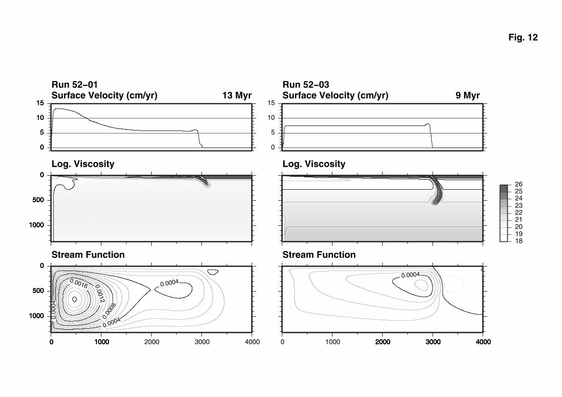
0

500

1000

0 1000

3000

0

500

1000

0 1000

3000

0

500

1000

0 1000

3000

0.00040.00

04

0.0004

0.00

08

0.0012

0.0016

0

500

1000

0 1000

3000

Stream Function0

500

1000

0 1000 2000 3000 4000

0

500

1000

0

500

1000

0

500

1000

0

500

1000

Log. Viscosity0

500

1000

0

5

10

15Surface Velocity (cm/yr)

0

5

10

1513 Myr

0

5

10

15

Run 52−01

0

5

10

15

2000 3000 4000

0

2000 3000 40002000 3000 4000

0

0.0004

2000 3000 4000

Stream Function

0 1000 2000 3000 4000

Log. Viscosity

Surface Velocity (cm/yr) 9 MyrRun 52−03

Fig. 12

0

5

10

15

181920212223242526

-0.4 0 0.4 0.8 1.2

0

200

400

600

800

1000

1200

1400

Relative horizontal velocity

Run 50-01 (30Myr, 2.3cm/yr)Run 50-01 (41 Myr, 4.1 cm/yr)Run 52-03 ( 5 Myr, 11.5 cm/yr)Run 52-03 (20 Myr, 3.8 cm/yr)

Velocity ratio

Dep

th (k

m)

Fig. 13

0

0.5

1

1.5

2

0 10 20 30 40 50

Mantle drag forces

DF+ Run 50-01DF- Run 50-01DF+ Run 52-03DF- Run 52-03

Forc

es (1

012 N

/m)

Time (Myr)

Fig. 14

0

2

4

6

8

10

0 50 100 150

Plate Velocity

100L-01 (VM-Ia, 300 MPa, 345)102L-01 (VM-IIIa, 300 MPa, 345)102L-02 (VM-IIIa, 300 MPa, 177)102L-03 (VM-IIIa, 600 MPa, 345)

Vel

ocity

(cm

/yr)

Time (Myr)

Fig. 16