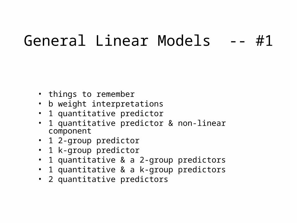
General Linear Models -- #1

• things to remember• b weight interpretations• 1 quantitative predictor• 1 quantitative predictor & non-linear component• 1 2-group predictor• 1 k-group predictor• 1 quantitative & a 2-group predictors • 1 quantitative & a k-group predictors• 2 quantitative predictors

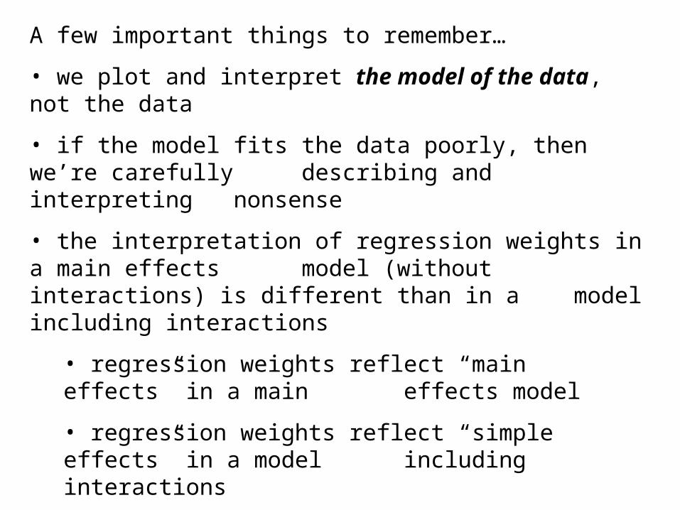
A few important things to remember…

• we plot and interpret the model of the data, not the data

• if the model fits the data poorly, then we’re carefully describing and interpreting nonsense

• the interpretation of regression weights in a main effects model (without interactions) is different than in a model including interactions

• regression weights reflect “main effects” in a maineffects model

• regression weights reflect “simple effects” in a modelincluding interactions

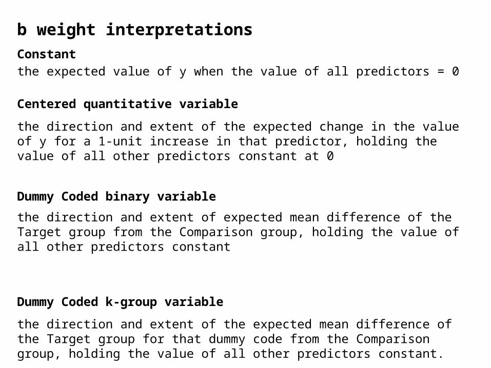
b weight interpretations

Constant

the expected value of y when the value of all predictors = 0

Centered quantitative variable

the direction and extent of the expected change in the value of y for a 1-unit increase in that predictor, holding the value of all other predictors constant at 0

Dummy Coded binary variable

the direction and extent of expected mean difference of the Target group from the Comparison group, holding the value of all other predictors constant

Dummy Coded k-group variable

the direction and extent of the expected mean difference of the Target group for that dummy code from the Comparison group, holding the value of all other predictors constant.

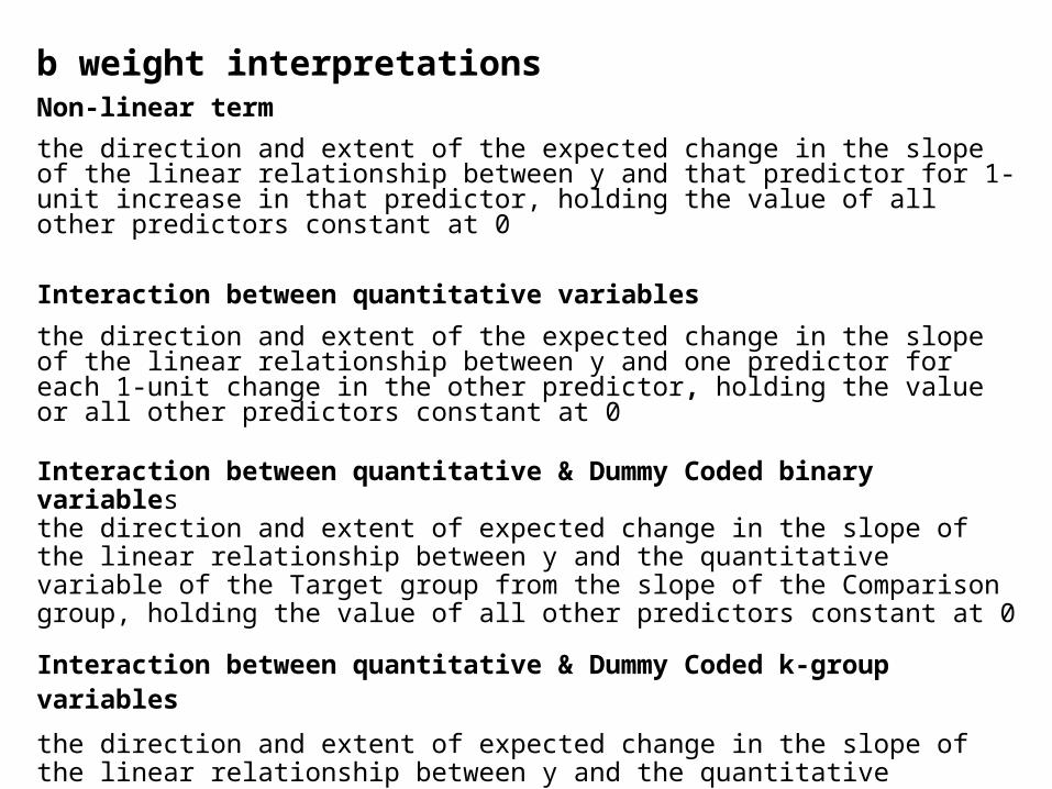
b weight interpretations Non-linear term

the direction and extent of the expected change in the slope of the linear relationship between y and that predictor for 1-unit increase in that predictor, holding the value of all other predictors constant at 0

Interaction between quantitative variables

the direction and extent of the expected change in the slope of the linear relationship between y and one predictor for each 1-unit change in the other predictor, holding the value or all other predictors constant at 0

Interaction between quantitative & Dummy Coded binary variablesthe direction and extent of expected change in the slope of the linear relationship between y and the quantitative variable of the Target group from the slope of the Comparison group, holding the value of all other predictors constant at 0

Interaction between quantitative & Dummy Coded k-group variables

the direction and extent of expected change in the slope of the linear relationship between y and the quantitative variable of the Target group for that dummy code from the slope of the Comparison group, holding the value of all other predictors constant at 0

0

10

20

30

4

0

50

60

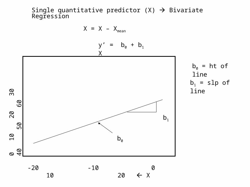
y’ = b0 + b1 X

b0

b1

-20 -10 0 10 20 X

b0 = ht of line

b1 = slp of line

X = X – Xmean

Single quantitative predictor (X) Bivariate Regression

0

10

20

30

4

0

50

60

y’ = b0 + b1 X

-20 -10 0 10 20 X

b0 = ht of line

b1 = slp of line

X = X – Xmean

Single quantitative predictor (X) Bivariate Regression

0

10

20

30

4

0

50

60

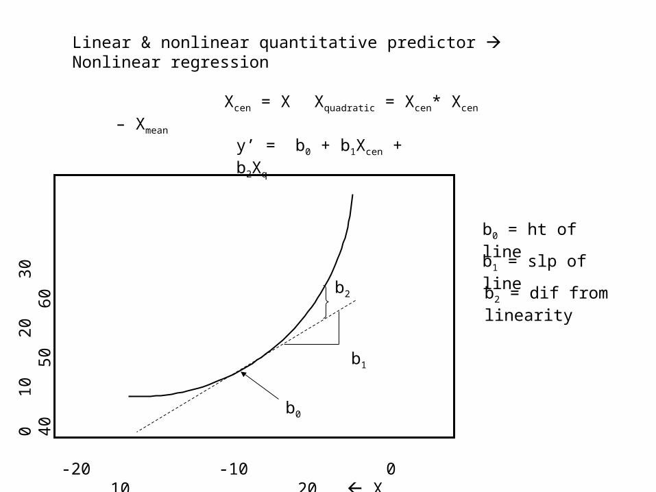
y’ = b0 + b1Xcen + b2Xq

b0

b1

Linear & nonlinear quantitative predictor Nonlinear regression

-20 -10 0 10 20 Xcen

Xquadratic = Xcen* Xcen

b2

Xcen = X – Xmean

b0 = ht of line

b1 = slp of line

b2 = dif from linearity

0

10

20

30

4

0

50

60

y’ = b0 + b1Xcen + b2Xq

Linear & nonlinear quantitative predictor Nonlinear regression

-20 -10 0 10 20 Xcen

Xquadratic = Xcen* Xcen Xcen = X – Xmean

b0 = ht of line

b1 = slp of line

b2 = dif from linearity

0

10

20

30

4

0

50

60

Cx

Tx

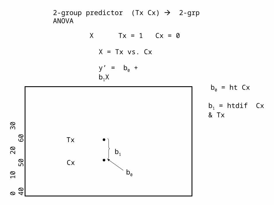
2-group predictor (Tx Cx) 2-grp ANOVA

b0 = ht Cx

b1 = htdif Cx & Tx

X Tx = 1 Cx = 0

X = Tx vs. Cx

b0

b1

y’ = b0 + b1X

0

10

20

30

4

0

50

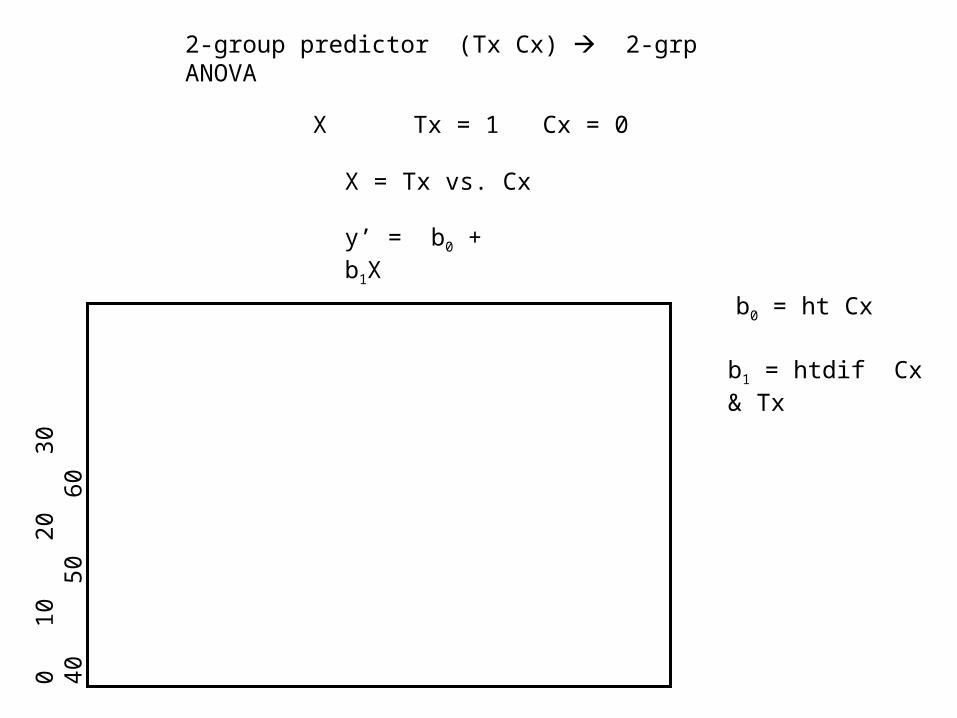
602-group predictor (Tx Cx) 2-grp ANOVA

b0 = ht Cx

b1 = htdif Cx & Tx

X Tx = 1 Cx = 0

X = Tx vs. Cx

y’ = b0 + b1X

0

10

20

30

4

0

50

60

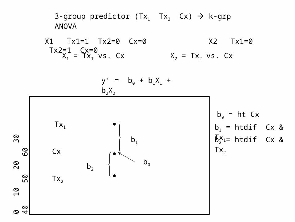
b2

Cx

Tx2

Tx1

b0 = ht Cx

b1 = htdif Cx & Tx1

b2 = htdif Cx & Tx2

3-group predictor (Tx1 Tx2 Cx) k-grp ANOVA

y’ = b0 + b1X1 + b2X2

X1 Tx1=1 Tx2=0 Cx=0 X2 Tx1=0 Tx2=1 Cx=0

X1 = Tx1 vs. Cx X2 = Tx2 vs. Cx

b0

b1

0

10

20

30

4

0

50

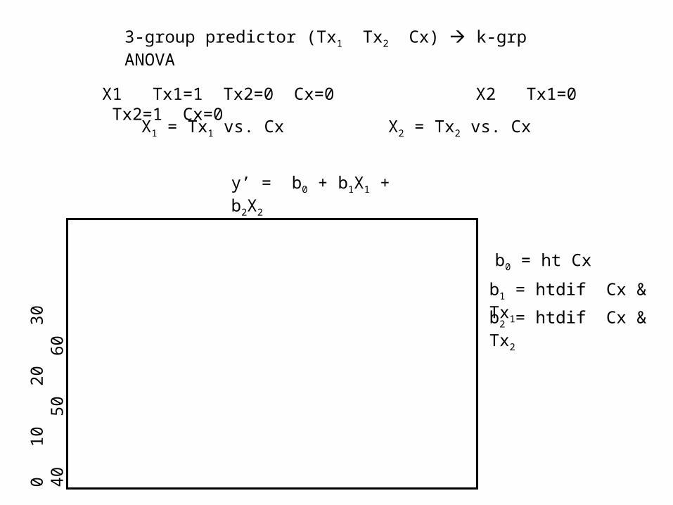
60 b0 = ht Cx

b1 = htdif Cx & Tx1

b2 = htdif Cx & Tx2

3-group predictor (Tx1 Tx2 Cx) k-grp ANOVA

y’ = b0 + b1X1 + b2X2

X1 Tx1=1 Tx2=0 Cx=0 X2 Tx1=0 Tx2=1 Cx=0

X1 = Tx1 vs. Cx X2 = Tx2 vs. Cx

0

10

20

30

4

0

50

60

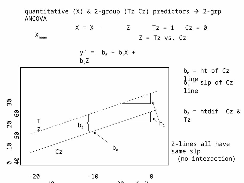
y’ = b0 + b1X + b2Z

b0

b1b2

Cz

Tz

quantitative (X) & 2-group (Tz Cz) predictors 2-grp ANCOVA

-20 -10 0 10 20 X

b0 = ht of Cz line

b1 = slp of Cz line

b2 = htdif Cz & Tz

X = X – Xmean Z Tz = 1 Cz = 0

Z = Tz vs. Cz

Z-lines all have same slp(no interaction)

0

10

20

30

4

0

50

60

y’ = b0 + b1X + b2Z

quantitative (X) & 2-group (Tz Cz) predictors 2-grp ANCOVA

-20 -10 0 10 20 X

b0 = ht of Cz line

b1 = slp of Cz line

b2 = htdif Cz & Tz

X = X – Xmean Z Tz = 1 Cz = 0

Z = Tz vs. Cz

Z-lines all have same slp(no interaction)

0

10

20

30

4

0

50

60

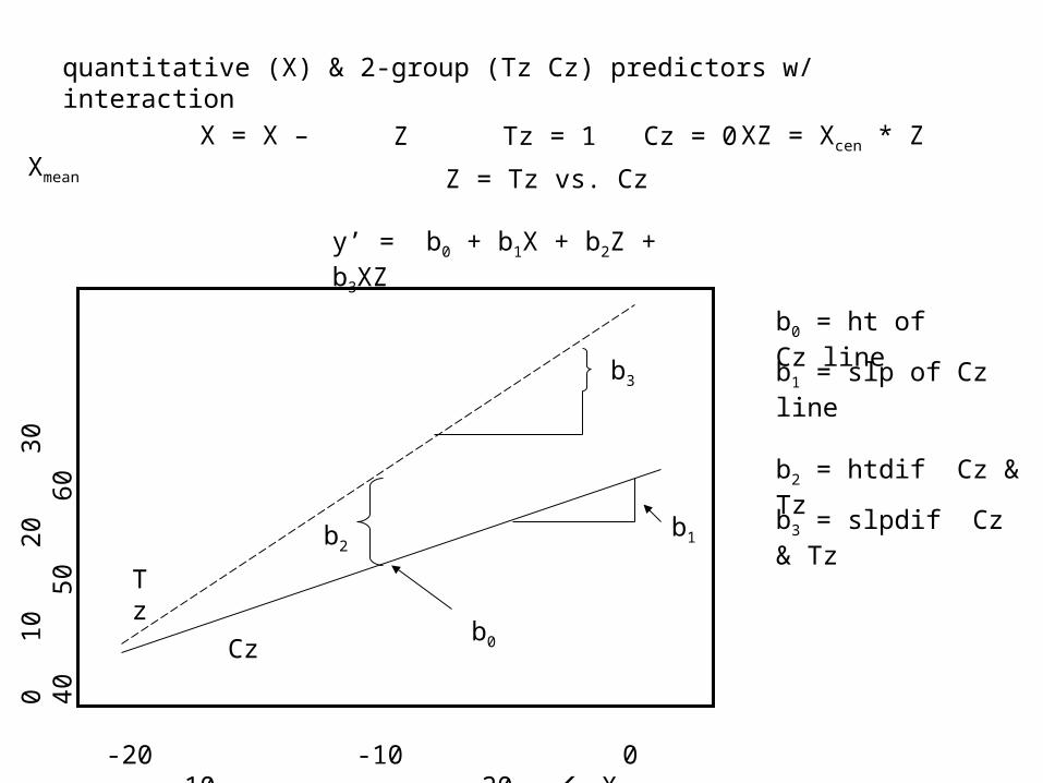
b0

b1b2

Cz

Tz

-20 -10 0 10 20 Xcen

XZ = Xcen * Z

b3

b0 = ht of Cz line

b1 = slp of Cz line

b2 = htdif Cz & Tz

b3 = slpdif Cz & Tz

quantitative (X) & 2-group (Tz Cz) predictors w/ interaction

y’ = b0 + b1X + b2Z + b3XZ

X = X – Xmean Z Tz = 1 Cz = 0

Z = Tz vs. Cz

0

10

20

30

4

0

50

60

-20 -10 0 10 20 Xcen

XZ = Xcen * Z

b0 = ht of Cz line

b1 = slp of Cz line

b2 = htdif Cz & Tz

b3 = slpdif Cz & Tz

quantitative (X) & 2-group (Tz Cz) predictors w/ interaction

y’ = b0 + b1X + b2Z + b3XZ

X = X – Xmean Z Tz = 1 Cz = 0

Z = Tz vs. Cz

0

10

20

30

4

0

50

60

b0

b1

b2

Cz

Tz2

Tz1

b3

-20 -10 0 10 20 X

b0 = ht of Cz line

b2 = htdif Cz & Tz1

b3 = htdif Cz & Tz2

b1 = slp of Cz line

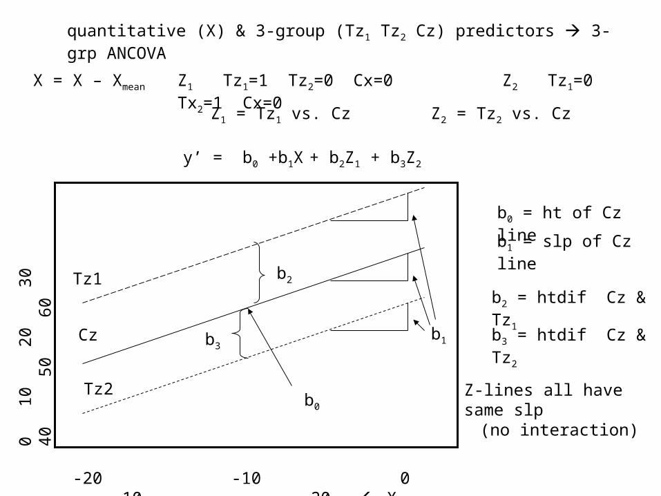
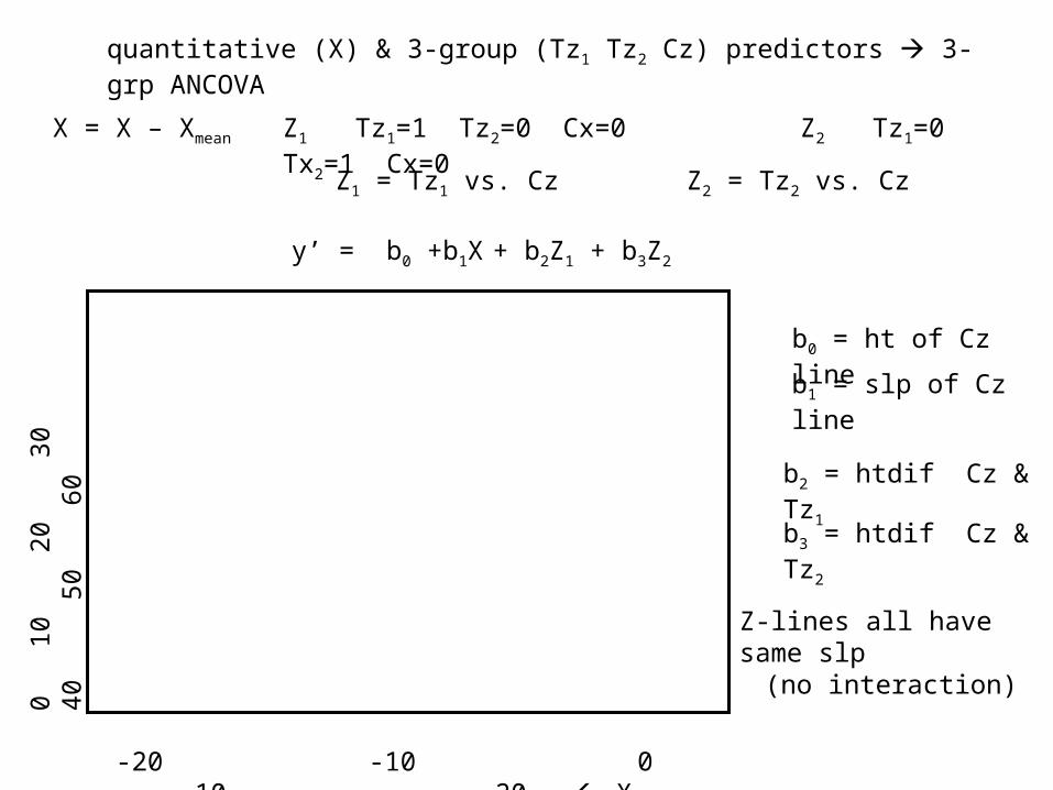
y’ = b0 +b1X + b2Z1 + b3Z2

Z1 = Tz1 vs. Cz Z2 = Tz2 vs. Cz

X = X – Xmean Z1 Tz1=1 Tz2=0 Cx=0 Z2 Tz1=0 Tx2=1 Cx=0

quantitative (X) & 3-group (Tz1 Tz2 Cz) predictors 3-grp ANCOVA

Z-lines all have same slp(no interaction)

0

10

20

30

4

0

50

60

-20 -10 0 10 20 X

b0 = ht of Cz line

b2 = htdif Cz & Tz1

b3 = htdif Cz & Tz2

b1 = slp of Cz line

y’ = b0 +b1X + b2Z1 + b3Z2

Z1 = Tz1 vs. Cz Z2 = Tz2 vs. Cz

X = X – Xmean Z1 Tz1=1 Tz2=0 Cx=0 Z2 Tz1=0 Tx2=1 Cx=0

quantitative (X) & 3-group (Tz1 Tz2 Cz) predictors 3-grp ANCOVA

Z-lines all have same slp(no interaction)

0

10

20

30

4

0

50

60

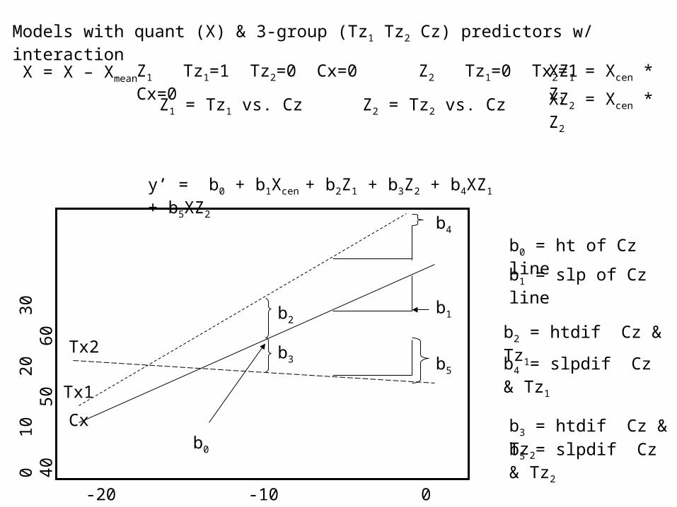
y’ = b0 + b1Xcen + b2Z1 + b3Z2 + b4XZ1 + b5XZ2

b0

b1b2

Cx

Tx1

Tx2 b3

-20 -10 0 10 20 Xcen

b0 = ht of Cz line

b2 = htdif Cz & Tz1

b3 = htdif Cz & Tz2

b1 = slp of Cz line

b4 = slpdif Cz & Tz1

b5 = slpdif Cz & Tz2

XZ1 = Xcen * Z1

XZ2 = Xcen * Z2

b4

b5

Models with quant (X) & 3-group (Tz1 Tz2 Cz) predictors w/ interaction

Z1 = Tz1 vs. Cz Z2 = Tz2 vs. Cz

X = X – Xmean Z1 Tz1=1 Tz2=0 Cx=0 Z2 Tz1=0 Tx2=1 Cx=0

0

10

20

30

4

0

50

60

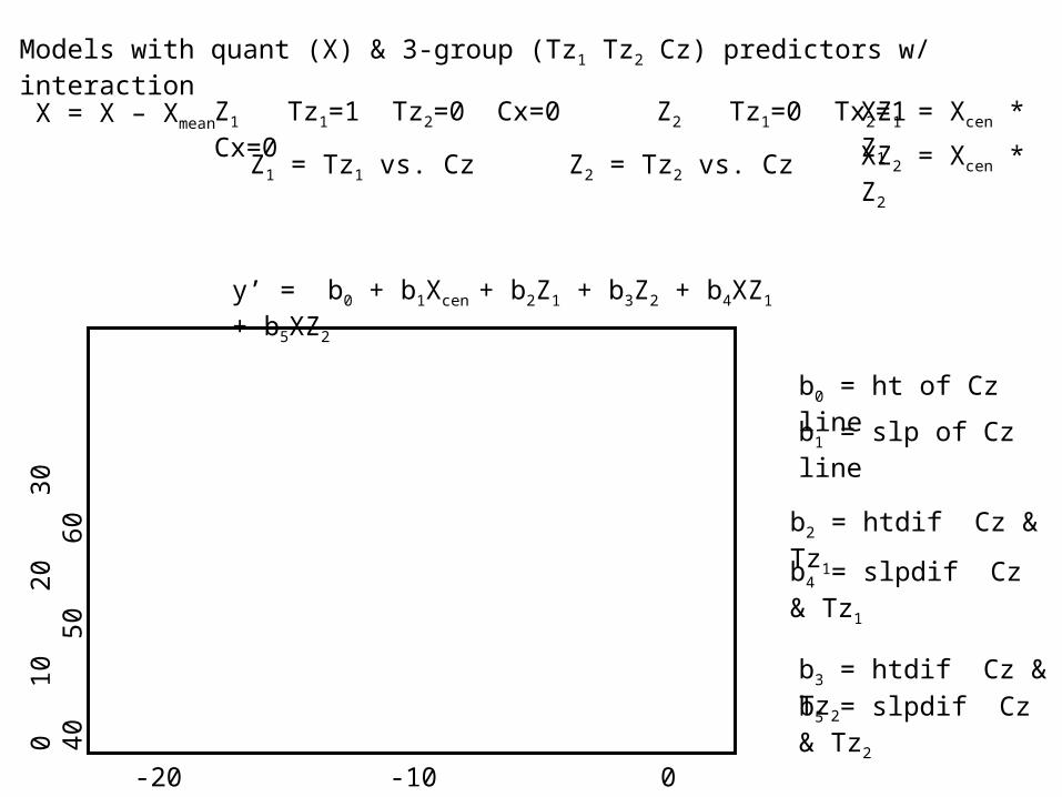
y’ = b0 + b1Xcen + b2Z1 + b3Z2 + b4XZ1 + b5XZ2

-20 -10 0 10 20 Xcen

b0 = ht of Cz line

b2 = htdif Cz & Tz1

b3 = htdif Cz & Tz2

b1 = slp of Cz line

b4 = slpdif Cz & Tz1

b5 = slpdif Cz & Tz2

XZ1 = Xcen * Z1

XZ2 = Xcen * Z2

Models with quant (X) & 3-group (Tz1 Tz2 Cz) predictors w/ interaction

Z1 = Tz1 vs. Cz Z2 = Tz2 vs. Cz

X = X – Xmean Z1 Tz1=1 Tz2=0 Cx=0 Z2 Tz1=0 Tx2=1 Cx=0

0

10

20

30

4

0

50

60

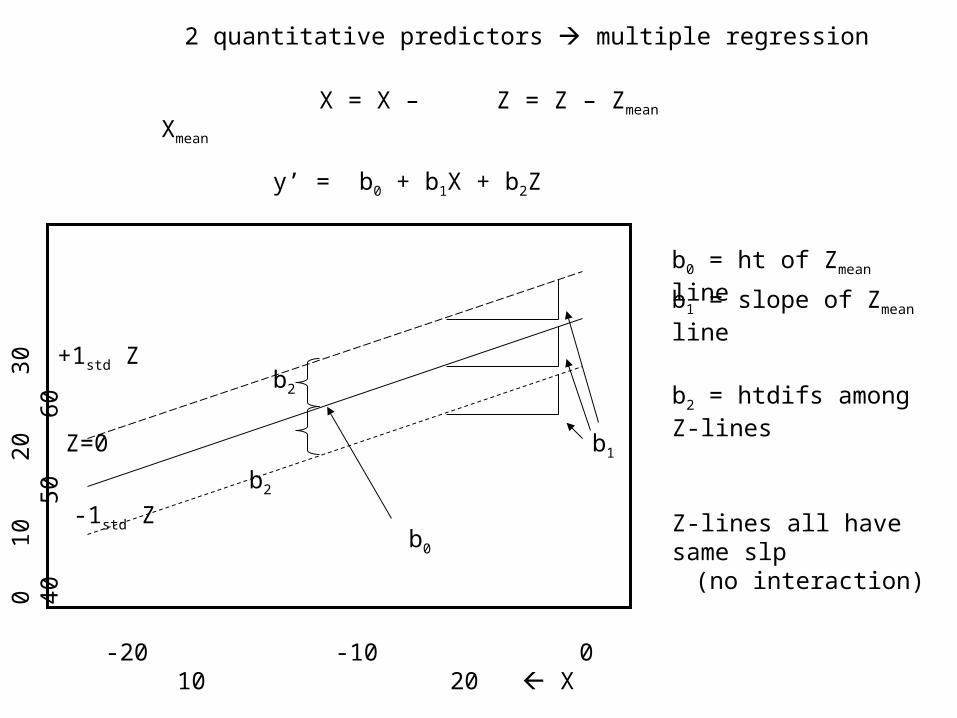
y’ = b0 + b1X + b2Z

b0

b1 b2Z=0

+1std Z

-1std Z

b2

Z = Z – Zmean

2 quantitative predictors multiple regression

-20 -10 0 10 20 X

b0 = ht of Zmean line

b1 = slope of Zmean line

b2 = htdifs among Z-lines

X = X – Xmean

Z-lines all have same slp(no interaction)

0

10

20

30

4

0

50

60

y’ = b0 + b1X + b2Z

Z = Z – Zmean

2 quantitative predictors multiple regression

-20 -10 0 10 20 X

b0 = ht of Zmean line

b1 = slope of Zmean line

b2 = htdifs among Z-lines

X = X – Xmean

Z-lines all have same slp(no interaction)

0

10

20

30

4

0

50

60

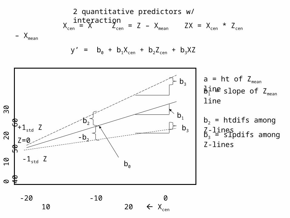
y’ = b0 + b1Xcen + b2Zcen + b3XZ

b0

b1

-b2Z=0

+1std Z

-1std Z

b2

Zcen = Z – Xmean

2 quantitative predictors w/ interaction

-20 -10 0 10 20 Xcen

a = ht of Zmean line

b1 = slope of Zmean line

b2 = htdifs among Z-lines

Xcen = X – Xmean ZX = Xcen * Zcen

b3

b3b3 = slpdifs among Z-lines

0

10

20

30

4

0

50

60

y’ = b0 + b1Xcen + b2Zcen + b3XZ

Zcen = Z – Xmean

2 quantitative predictors w/ interaction

-20 -10 0 10 20 Xcen

a = ht of Zmean line

b1 = slope of Zmean line

b2 = htdifs among Z-lines

Xcen = X – Xmean ZX = Xcen * Zcen

b3 = slpdifs among Z-lines

0

10

20

30

4

0

50

60

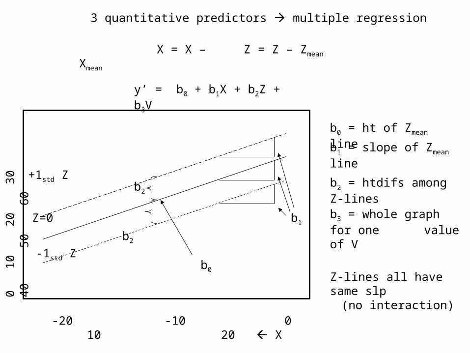
y’ = b0 + b1X + b2Z + b3V

b0

b1 b2Z=0

+1std Z

-1std Z

b2

Z = Z – Zmean

3 quantitative predictors multiple regression

-20 -10 0 10 20 X

b0 = ht of Zmean line

b1 = slope of Zmean line

b2 = htdifs among Z-lines

X = X – Xmean

Z-lines all have same slp(no interaction)

b3 = whole graph for one value of V