prediction model of air pollutant levels using linear ... · predictor variables to be imputed into...

Abstract—The prediction of each of air pollutants as

dependent variable was investigated using lag-1(30 minutes

before) values of air pollutants (nitrogen dioxide, NO2,

particulate matter 10um, PM10, and ozone, O3) and

meteorological factors and temporal variables as independent

variables by taking into account serial error correlations in the

predicted concentration. Alternative variables selection based

on independent component analysis (ICA) and principal

component analysis (PCA) were used to obtain subsets of the

predictor variables to be imputed into the linear model. The

data was taken from five monitoring stations in Surabaya City,

Indonesia with data period between March-April 2002. The

regression with variables extracted from ICA was the worst

model for all pollutants NO2, PM10, and O3 as their residual

errors were highest compared with other models. The

prediction of one-step ahead 30-mins interval of each pollutant

NO2, PM10, and O3 was best obtained by employing original

variables combination of air pollutants and meteorological

factors. Besides the importance of pollutants interaction and

meteorological aspects into the prediction, the addition spatial

source such as wind direction from each monitoring station has

significant contribution to the prediction as the emission

sources are different for each station.

Index Terms—Linear regression, principal component

regression, independent component regression, air quality

prediction, generalized least square.

I. INTRODUCTION

Air pollution prevention has been the leading concern of

citites in most developing countries, in particular in Surabaya

where the vehicle ownerships increase sharply every year. As

a result, the emission of traffic-related pollutants e.g., NO2,

PM10 increase. Furthermore, the reaction of NO2 with NO

will result in the ozone (O3) formation. Therefore, it is

mandatory to keep the concentration of these pollutants

below permissible level in which the concentration will not

affect humans health. High concentration of NO2 and PM10 is

known to affect human health, whereas O3 is responsible for

photochemical smog [1]. High concentration of PM10

increase the risk of cardiovascular and respiratory diseases

[2]. The prediction model is required to ensure these limits

are not surpassed, and if not, the information of the prediction

will be crucial for future environmental policies.

In recent time, there have been many attempt to analyze the

Manuscript received May 2, 2014; revised August 26, 2014. This work

was supported by the Global Environmental Leaders (GELs) Program of

Graduate Institute of International and Development, Hiroshima University

and Directorate of General Directorate of Higher Education, Ministry of

Education, Republic of Indonesia for providing full financial support during

research in the Hiroshima University.

The authors are with the Graduate School of International Development

and Cooperation, Hiroshima University, Japan (e-mail: d115407@

Hiroshima-u.ac.jp, [email protected], [email protected]).

concentration of air pollutants and explore them to build

short-term forecast of concentrations. Linear and non-linear

models were developed, however, there was no significance

difference noted between non-linear and linear models [3].

Reference [4] used a forecasting model called Bayesian

hierarchical technique to predict CO, NOx, and dust fall.

Reference [3] compared five linear models to predict daily

mean of PM10 concentrations in one site in Oporto

Metropolitan Area. However, spatial variability were not

concerned on that study and the regression with variables

obtained independent component analysis performed the

worse. Reference [5] employed Artificial Neural Network

(ANN) to predict CO, NO2, PM10 and O3 concentrations and

the performance was better compared with multiple linear

regression. On this research, wind direction was considered

as independent variables but they did not separate the effect

of wind direction to each prediction of pollutant, moreover,

serial error correlation due to time series model was not taken

into account which might cause result bias. Reference [6]

also used ANN to predict pollutants, but they noted less

accuracy for O3 prediction in Tehran, Iran.

The time series is an appropriate model which avoids the

problems of geographical aspects. However, the trends

observed in a pollution data presents serrial error

autocorrelation which generates problems in interpretation,

analysis, and prediction [7]. Many researchers have

performed the forecasting by regression technique but

unfortunately many authors did not account for serial error

autocorrelation.

Moreover, in a regression analysis, the correlation between

independent variables (multicollinearity) may pose a serious

difficulty in the interpretation of which predictors are the

most influential to the response variables [8]. One way to

remove such multicollinearity is using component analysis

method, in this case widely used a Principal Component

Analysis (PCA), and the newly emerged one Independent

Component Analysis (ICA). Even though these two methods

have their own approach, the goal is similar is to build

components that are statistically independent with each other.

In regression analysis, this is particularly very useful and

become good input as predictors in a regression model since

they optimize spatial patterns and remove complexity due to

multicollinearity [8], [9]. ICR and PCR have been widely

used in particular for plant study [9], dam deformation study

[10], air pollutants in subway [11], air quality management

[2], [3], [12], and O3 prediction [1].

In this paper, we will predict one-step (next 30mins) ahead

three pollutants, namely, NO2, PM10, and O3 concentrations

by including some spatial and temporal factors. Important

variables which are also included are six air pollutants (NO2,

NO, O3, SO2, CO, PM10, and meteorological factors (wind

speed, wind direction for each station, solar gradiation,

Prediction Model of Air Pollutant Levels Using Linear

Model with Component Analysis

Arie Dipareza Syafei, Akimasa Fujiwara, and Junyi Zhang

International Journal of Environmental Science and Development, Vol. 6, No. 7, July 2015

519DOI: 10.7763/IJESD.2015.V6.648

mailto:[email protected]

humidity, and temperatures). We employ a Generalized Least

Square (GLS) model with taking into concern the series of

error autocorrelation. As far as author concerns this study is

the first one applied in current city and country and its

ultimate benefit that we may be able to show the key factors

of a model which can be applied further into other areas and

regions, in particular within Indonesia.

II. MATERIALS AND DATA

We make use of 30-mins interval concentrations of NO,

NO2, O3, SO2, CO, and PM10 as well as meteorological

factors that consist of wind direction, wind speed (m/s), solar

gradiation (W/m2), humidity (%), and temperatures (oC).

These data were obtained from Air Quality Laboratory of

Environmental Agency in Surabaya City, recorded from five

monitoring stations installed. These five stations represent:

city center (Ketabang Kali – Station 1), trading zone (Perak –

Station 2), suburban (west side of Surabaya, Sukomanunggal

– Station 3), near highway zone (Gayungsari – Station 4), and

suburban (east side of Surabaya, Sukolilo – Station 5).

In the present study we attempt to predict NO2, PM10, and

O3 using GLS model using the data taken from March 2002 to

April 2002, with total 14635 observations (five stations), as

training set, whereas the test set, which is not used for

parameter estimation, was taken from May 2002. Missing

values were treated using Expectation Maximization based

algorithm by package Amelia run through R open source

program [13]. Table I shows each mean value, standard

deviation, and median of each pollutant concentrations (in

ug/m3) from five stations in Surabaya. It can be seen that

average emission that is related to traffic (NO2) was high in

city center and low in suburban2 on the east side of Surabaya.

With regards of PM10, high average concentration was found

on suburban1 on west side of Surabaya. Interestingly, mean

value of O3 concentration was high on highway zone

suggesting high reaction rate between NO and NO2 due to

traffic flow.

TABLE I: DESCRIPTIVE STATISTICS OF LEVELS OF POLLUTANTS IN SURABAYA FROM FIVE MONITORING STATIONS (UG/M3)

Description City Center Trading Suburban1 Near Highway Suburban2

NO2 Min 1.603 0.335 1.175 0.48 0.055

Max 12.309 11.577 10.013 16.024 8.538

Mean 5.487 4.745 4.85 5.266 4.151

Standard Deviation 1.518 1.703 1.503 1.758 1.62

PM10 Min 0.656 0.1 0.317 0.541 0.117

Max 17.38 48.799 17.689 48.99 14.979

Mean 7.137 7.673 7.857 7.488 6.79


O3 Min 1.558 0.042 0.01 0.042 0.174

Max 15.612 13.613 13.976 26.088 14.453

Mean 6.067 6.305 5.614 4.372 6.864


GLSs were then fitted, with square-root transformed of

each pollutant (NO2, O3, or PM10) as the dependent variable.

The explanatory variables were functions of lag-1 30-mins

interval of pollutant levels: NO2, NO, O3, SO2, CO, PM10,

wind speed, solar gradiation, humidity, temperatures, status

of day (weekends, workdays as base reference), peak time of

morning and afternoon session (non-peak time as base

reference with peak time morning is between 630am to 9am

and in the evening between 430pm to 7pm), holidays, spatial

covariates of zones: trading, suburban1, highway, suburban2,

with city center as base reference, and wind direction. For

wind direction we created eight variables representing

direction as dummy variables. They are north, northeast, east,

southeast, east, south, southwest, west, and northwest, with

north as base reference. These variable values are different

for each station, thus creating more 35 wind direction

variables for model input. All air pollutants and wind speed

were all square-root transformed as standard procedures to

stabilize the variance. Each dependent variable is predicted

by the interaction of other pollutants one-step backward (last

30-mins concentration). The three pollutants were considered

in three separate GLS models because of their substantial

correlation. On a second and third model, the variables of six

air pollutants and four meteorological factors were replaced

by components extracted from an ICA and PCA. Total there

were 10 ICs and 10 PCs were obtained and used as predictor

variabels along with other independent variables as described

above.

III. MODELS

A. Generalized Least Square

We employ a Generalized Least Squares (GLS) model to

formula the mixed linear effect of predictor variables towards

the concentration of pollutants, following the equation:

Xy (1)

where y is n × 1 response variable (pollutant) and X is an n × p

matrix, β is a p × 1 vector of estimated parameters, and ε is n

× 1 vector of errors. With the assumption that

nn IN 2,0~ , we can estimate ordinary least square

estimator of β:

yXXXOLS ''1

(2)

With covariance matrix

12 '

XXV OLS (3)


520

When the error covariance Σ positive-definite and

symmetric and its diagonal entries Σ correspond to

non-constant error variances, and nonzero off-diagonal

entries are associated with correlated errors, we can estimate

the log-likelihood of the model, given that Σ is known:

detlog2

ee

nLLog

XyXy '2

1 (4)

The function is maximized by the GLS estimator of β:

yXXXGLS111 '' (5)

With covariance matrix:

11' XXV GLS (6)

However, in the application, the matrix of Σ is not known

and therefore must be estimated from the data with the

regression coefficients, β.

In time series data, though, there is a concern of error

correlation. Assuming that all errors have same expectation

and same variance, the covariance of two errors depends on

their separation s in time:

ssttstt CC 2,, (7)

where s is the error autocorrelation at lag s. The

error-covariance matrix will become:

P

nnn

n

n

n

2

321

312

211

121

2

1

1

...1

1

(8)

For stationary time-series, we apply first-order

auto-regressive process, AR(1) for autocorrelated regression

errors:

ttt v 1 (9)

Under this model, the tv is assumed to be Gaussian white

noise, 11 t , ss , and 222 1 v , along

with the time run, the error autocorrelations s will decay

exponentially as s increases to 0. A GLS model is run through

a gls command under nlme library package within R open

source software.

B. Independent Component Analysis

In ICA, the input variables are regarded as linear

combinations of latent variables which are considered

independent and non-Gaussian. ICA establishes independent

components from original variables. The concept of ICA is

regarded to be able in explaining more for variable

relationship because independence is a high-order statistic

that is in favor over orthogonality [9]. The GLS regression

forms relationship between response variable (y) and the ICs

from ICA along with other explanatory variables (e.g., days

in week, season). A typical ICA model is expressed as:

X = SA (10)

X is observation matrix, derived through the mixing of an

n-dimensional source matrix, S = (s1, …, sn)T, with temporal

dimension of l, referred to ICs, with n is independent

components extracted. A is the mixing matrix of dimension n

× n or m × n where m ≤ n. The objective of ICA is to estimate

A and S, knowing only the observations matrix X. The present

study uses Fast ICA algorithm to estimate A and S from

observations X. The S components will be used as input

variables in the model. A fast ICA function within R program

was used to obtain ICs. For forecasting purpose, the

following formula is used to obtain ICs for input to the

prediction model:

XA-1 = S (11)

X is lag-1 independent variables whereas A is the inverse of

loading matrix obtained from training set data. There were 10

ICs obtained as input variables.

C. Principal Component Analysis

PCA creates principal components (PCs) that are

orthogonal and uncorrelated and linear combinations of the

original variables. The first PC is the one that has the largest

portion of original data variability. A varimax rotation is

commonly used to obtain rotated factor weight loadings that

represent effect of each each variable in one particular PC.

MPC regression examines a relationship between the output

variable (y) and the PCs obtained from explanatory variables

(air pollutants: NO, NO2, O3, SO2, CO, and PM10, and

meteorological factors: wind speed, solar gradiation,

humidity, and temperatures). The estimation procedure is

given in the following equations:

m

kkjikij xwPC

1 (12)

where PCij is the PC score for ith component and j-th object.

The loading weight is represented by wik for k-th variable

variable on the i-th component, and xkj is the standardized

value of k-th variable for the j-th observation [14]. A PCA is

run using prcomp function within R open source program. To

obtain PCs for prediction purposes, the xkj were simply lag-1

independent variables.

IV. MODEL TERMS, FORECASTING, AND PERFORMANCE

INDEXES

In the present study we define the term model as follow:

Model 1 is a Generalized Least Square (GLS) model with

original square-root transformed independent variables (air

pollutants and meteorological factors). Model 2 refers to that

predictor variables are replaced by components extracted

from ICA. Model 3 refers to a model with the predictor


521

variables are replaced by components obtained from PCA.

Forecasting of the model was done by comparing fitted

values and observation values in Station 1 (city center) and

Station 5 (suburban2). The three models were compared and

judged using these statistical performance index: mean error

(ME), mean absolute error (MAE), root mean square error

(RMSE), and R2, that are commonly used in many literatures.

ME is useful to obtain whether the fitted values overestimate

or underestimate. MAE and RMSE measure the magnitude of

difference between predicted values and observed values, the

lower the better. The R2 indicate percentage of which

variance can be explained by variables.

V. RESULTS AND DISCUSSIONS

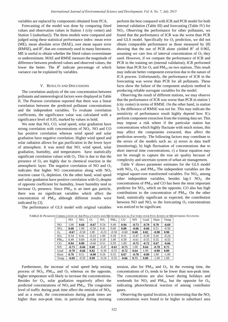
The correlation analysis of the raw concentration between

pollutants and meteorological factors were displayed in Table

II. The Pearson correlation reported that there was a linear

correlation between the predicted pollutant concentrations

and the independent variables. To evaluate correlation

coefficients, the significance value was calculated with a

significance level of 0.05, marked by values in bold.

We note that NO, CO, wind speed, solar gradiation have

strong correlation with concentrations of NO2. NO and CO

has positive correlation whereas wind speed and solar

gradiation have negative correlation. Higher wind speed and

solar radiation allows for gas purification in the lower layer

of atmosphere. It was noted that NO, wind speed, solar

gradiation, humidity, and temperatures have statistically

significant correlation values with O3. This is due to that the

presence of O3 are highly due to chemical reaction in the

atmospheric layer. The negative correlation of NO and O3

indicates that higher NO concentration along with NO2

reaction cause O3 depletion. On the other hand, wind speed

and solar gradiation have positive correlation with O3 despite

of opposite coefficient for humidity, lower humidity tend to

increase O3 presence. Since PM10 is an inert gas particle,

there was no significant variables which affect the

concentration of PM10 although different results were

indicated by [3].

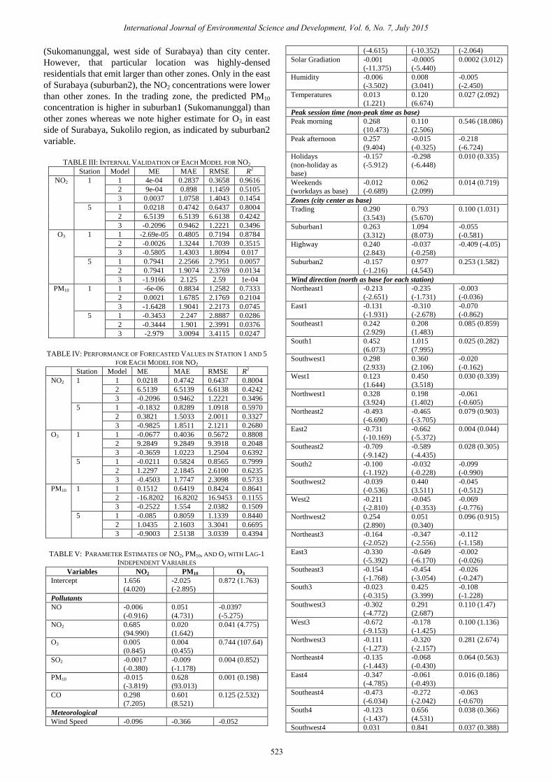
The performance of GLS model with original variables

perform the best compared with ICR and PCR model for both

internal validation (Table III) and forecasting (Table IV) for

NO2. Observing the performance for other pollutants, we

found that the performance of ICR was the worst than PCR

and GLS model. Specifically for O3 prediction, we did not

obtain comparable performance as those measured by [8]

showing that the use of PCR alone yielded R2 of 0.965,

assuming we care less of interval concentration of O3 they

used. However, if we compare the performance of ICR and

PCR in the training set (internal validation), ICR performed

better than PCR for O3 and PM10 on two stations. This result

may indicate better component extraction due to the nature of

ICA process. Unfortunately, the performance of ICR in the

forecasting was worse than PCR for all pollutants. These

facts show the failure of the component analysis method in

producing reliable surrogate variables for the model.

Observing the result of different stations, we may observe

that the performance of ICR was worse than PCR in station 1

(city center) in terms of RMSE. On the other hand, in station

5, the difference of RMSE was not far. This may indicate the

sensitivity of performance result highly depend how ICs

perform component extraction from the training data set. This

may impose a risk where if the particular station has

concentrations which highly fluctuate with much noises, this

may affect the components extracted, thus affect the

prediction severely. The following factors may contribute to

the errors of the models such as: a) errors in data itself

(monitoring), b) high fluctuation of concentrations due to

short interval time concentrations, c) a linear equation may

not be enough to capture the true air quality because of

complexity and uncertain system of urban air management.

Table V shows parameter estimates for the GLS model

with NO2, O3, and PM10 The independent variables are the

original square-root transformed variables. For NO2, among

other independent variables, besides lag-1 NO2, the

concentrations of PM10 and CO has been the most important

predictor for NO2, which on the opposite, CO also has high

contributions to the concentration of PM10. On the other

hand, statistically significant as expected, the contribution

between NO and NO2 to the forecasting O3 concentrations

was noticed to be significant.

TABLE II: PEARSON CORRELATION OF AIR POLLUTANTS AND METEOROLOGICAL FACTORS OVER FIVE ZONES OF MONITORING STATIONS

NO NO2 O3 SO2 PM10 CO WS Grad Hum Temp

NO 1.00 0.68 -0.67 0.54 0.49 0.94 -0.73 -0.70 0.70 -0.69

NO2 0.68 1.00 -0.50 0.41 0.60 0.80 -0.66 -0.66 0.51 -0.50

O3 -0.67 -0.50 1.00 -0.23 -0.50 -0.60 0.68 0.82 -0.90 0.90

SO2 0.54 0.41 -0.23 1.00 0.18 0.51 -0.47 -0.30 0.26 -0.24

PM10 0.49 0.60 -0.50 0.18 1.00 0.59 -0.61 -0.55 0.55 -0.55

CO 0.94 0.80 -0.60 0.51 0.59 1.00 -0.75 -0.72 0.67 -0.66

WS -0.73 -0.66 0.68 -0.47 -0.61 -0.75 1.00 0.64 -0.78 0.75

Grad -0.70 -0.66 0.82 -0.30 -0.55 -0.72 0.64 1.00 -0.89 0.89

Hum 0.70 0.51 -0.90 0.26 0.55 0.67 -0.78 -0.89 1.00 -1.00

Temp -0.69 -0.50 0.90 -0.24 -0.55 -0.66 0.75 0.89 -1.00 1.00

Furthermore, the increase of wind speed help mixing

process of NO2, PM10, and O3 whereas on the opposite,

higher temperature will likely to increase the concentrations.

Besides for O3, solar gradiation negatively affect the

predicted concentrations of NO2 and PM10. The congestion

level of traffic during peak time affect the emission of NO2,

and as a result, the concentrations during peak times are

higher than non-peak time, in particular during morning

session, also for PM10 and O3. In the evening time, the

concentrations of O3 tends to be lower than non-peak time.

The concentrations are also lower during holidays and

weekends for NO2 and PM10, but the opposite for O3,

indicating photochemical reaction of among contributor

gases.

Observing the spatial location, it is interesting that the NO2

concentrations were found to be higher in suburban1 area


522

(Sukomanunggal, west side of Surabaya) than city center.

However, that particular location was highly-densed

residentials that emit larger than other zones. Only in the east

of Surabaya (suburban2), the NO2 concentrations were lower

than other zones. In the trading zone, the predicted PM10

concentration is higher in suburban1 (Sukomanunggal) than

other zones whereas we note higher estimate for O3 in east

side of Surabaya, Sukolilo region, as indicated by suburban2

variable.

TABLE III: INTERNAL VALIDATION OF EACH MODEL FOR NO2

Station Model ME MAE RMSE R2

NO2 1 1 4e-04 0.2837 0.3658 0.9616

2 9e-04 0.898 1.1459 0.5105

3 0.0037 1.0758 1.4043 0.1454

5 1 0.0218 0.4742 0.6437 0.8004

2 6.5139 6.5139 6.6138 0.4242

3 -0.2096 0.9462 1.2221 0.3496

O3 1 1 -2.69e-05 0.4805 0.7194 0.8784

2 -0.0026 1.3244 1.7039 0.3515

3 -0.5805 1.4303 1.8094 0.017

5 1 0.7941 2.2566 2.7951 0.0057

2 0.7941 1.9074 2.3769 0.0134

3 -1.9166 2.125 2.59 1e-04

PM10 1 1 -6e-06 0.8834 1.2582 0.7333

2 0.0021 1.6785 2.1769 0.2104

3 -1.6428 1.9041 2.2173 0.0745

5 1 -0.3453 2.247 2.8887 0.0286

2 -0.3444 1.901 2.3991 0.0376

3 -2.979 3.0094 3.4115 0.0247

TABLE IV: PERFORMANCE OF FORECASTED VALUES IN STATION 1 AND 5

FOR EACH MODEL FOR NO2

Station Model ME MAE RMSE R2

NO2 1 1 0.0218 0.4742 0.6437 0.8004

2 6.5139 6.5139 6.6138 0.4242

3 -0.2096 0.9462 1.2221 0.3496

5 1 -0.1832 0.8289 1.0918 0.5970

2 0.3821 1.5033 2.0011 0.3327

3 -0.9825 1.8511 2.1211 0.2680

O3 1 1 -0.0677 0.4036 0.5672 0.8808

2 9.2849 9.2849 9.3918 0.2048

3 -0.3659 1.0223 1.2504 0.6392

5 1 -0.0211 0.5824 0.8565 0.7999

2 1.2297 2.1845 2.6100 0.6235

3 -0.4503 1.7747 2.3098 0.5733

PM10 1 1 0.1512 0.6419 0.8424 0.8641

2 -16.8202 16.8202 16.9453 0.1155

3 -0.2522 1.554 2.0382 0.1509

5 1 -0.085 0.8059 1.1339 0.8440

2 1.0435 2.1603 3.3041 0.6695

3 -0.9003 2.5138 3.0339 0.4394

TABLE V: PARAMETER ESTIMATES OF NO2, PM10, AND O3 WITH LAG-1

INDEPENDENT VARIABLES

Variables NO2 PM10 O3

Intercept 1.656

(4.020)

-2.025

(-2.895)

0.872 (1.763)

Pollutants

NO -0.006

(-0.916)

0.051

(4.731)

-0.0397

(-5.275)

NO2 0.685

(94.990)

0.020

(1.642)

0.041 (4.775)

O3 0.005

(0.845)

0.004

(0.455)

0.744 (107.64)

SO2 -0.0017

(-0.380)

-0.009

(-1.178)

0.004 (0.852)

PM10 -0.015

(-3.819)

0.628

(93.013)

0.001 (0.198)

CO 0.298

(7.205)

0.601

(8.521)

0.125 (2.532)

Meteorological

Wind Speed -0.096 -0.366 -0.052

(-4.615) (-10.352) (-2.064)

Solar Gradiation -0.001

(-11.375)

-0.0005

(-5.440)

0.0002 (3.012)

Humidity -0.006

(-3.502)

0.008

(3.041)

-0.005

(-2.450)

Temperatures 0.013

(1.221)

0.120

(6.674)

0.027 (2.092)

Peak session time (non-peak time as base)

Peak morning 0.268

(10.473)

0.110

(2.506)

0.546 (18.086)

Peak afternoon 0.257

(9.404)

-0.015

(-0.325)

-0.218

(-6.724)

Holidays

(non-holiday as

base)

-0.157

(-5.912)

-0.298

(-6.448)

0.010 (0.335)

Weekends

(workdays as base)

-0.012

(-0.689)

0.062

(2.099)

0.014 (0.719)

Zones (city center as base)

Trading 0.290

(3.543)

0.793

(5.670)

0.100 (1.031)

Suburban1 0.263

(3.312)

1.094

(8.073)

-0.055

(-0.581)

Highway 0.240

(2.843)

-0.037

(-0.258)

-0.409 (-4.05)

Suburban2 -0.157

(-1.216)

0.977

(4.543)

0.253 (1.582)

Wind direction (north as base for each station)

Northeast1 -0.213

(-2.651)

-0.235

(-1.731)

-0.003

(-0.036)

East1 -0.131

(-1.931)

-0.310

(-2.678)

-0.070

(-0.862)

Southeast1 0.242

(2.929)

0.208

(1.483)

0.085 (0.859)

South1 0.452

(6.073)

1.015

(7.995)

0.025 (0.282)

Southwest1 0.298

(2.933)

0.360

(2.106)

-0.020

(-0.162)

West1 0.123

(1.644)

0.450

(3.518)

0.030 (0.339)

Northwest1 0.328

(3.924)

0.198

(1.402)

-0.061

(-0.605)

Northeast2 -0.493

(-6.690)

-0.465

(-3.705)

0.079 (0.903)

East2 -0.731

(-10.169)

-0.662

(-5.372)

0.004 (0.044)

Southeast2 -0.709

(-9.142)

-0.589

(-4.435)

0.028 (0.305)

South2 -0.100

(-1.192)

-0.032

(-0.228)

-0.099

(-0.990)

Southwest2 -0.039

(-0.536)

0.440

(3.511)

-0.045

(-0.512)

West2 -0.211

(-2.810)

-0.045

(-0.353)

-0.069

(-0.776)

Northwest2 0.254

(2.890)

0.051

(0.340)

0.096 (0.915)

Northeast3 -0.164

(-2.052)

-0.347

(-2.556)

-0.112

(-1.158)

East3 -0.330

(-5.392)

-0.649

(-6.170)

-0.002

(-0.026)

Southeast3 -0.154

(-1.768)

-0.454

(-3.054)

-0.026

(-0.247)

South3 -0.023

(-0.315)

0.425

(3.399)

-0.108

(-1.228)

Southwest3 -0.302

(-4.772)

0.291

(2.687)

0.110 (1.47)

West3 -0.672

(-9.153)

-0.178

(-1.425)

0.100 (1.136)

Northwest3 -0.111

(-1.273)

-0.320

(-2.157)

0.281 (2.674)

Northeast4 -0.135

(-1.443)

-0.068

(-0.430)

0.064 (0.563)

East4 -0.347

(-4.785)

-0.061

(-0.493)

0.016 (0.186)

Southeast4 -0.473

(-6.034)

-0.272

(-2.042)

-0.063

(-0.670)

South4 -0.123

(-1.437)

0.656

(4.531)

0.038 (0.366)

Southwest4 0.031 0.841 0.037 (0.388)


523

(0.396) (6.257)

West4 -0.043

(-0.586)

1.121

(9.024)

0.002 (0.028)

Northwest4 -0.171

(-1.974)

0.162

(1.114)

0.077 (0.736)

Northeast5 -0.031

(-0.231)

-0.362

(-1.629)

-0.335

(-1.999)

East5 -0.034

(-0.282)

-0.217

(-1.075)

-0.042

(-0.275)

Southeast5 -0.012

(-0.098)

-0.307

(-1.546)

-0.031

(-0.203)

South5 0.126

(1.043)

-0.175

(-0.875)

0.108 (0.714)

Southwest5 0.023

(0.187)

-0.460

(-2.283)

0.202 (1.323)

West5 0.018

(0.145)

-0.165

(-0.796)

0.084 (0.536)

Northwest5 -0.042

(-0.298)

-0.556

(-2.427)

0.149 (0.853)

AR(1) parameter

estimates

-0.224 -0.140 -0.364

AIC 44441.81 58558.89 52075.29

BIC 44866.7 58983.79 52500.19

Log likelihood -22164.9 -29223.44 -25981.65

t-value is listed inside bracket

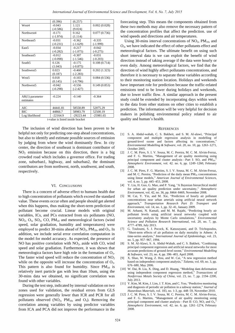
The inclusion of wind direction has been proven to be

helpful not only for predicting one-step ahead concentrations,

but also to identify and estimate possible sources of emission

by judging from where the wind dominantly flew. In city

center, the direction of southeast is dominant contributor of

NO2 emission because on this direction, there is a big

crowded road which includes a governor office. For trading

zone, suburban1, highway, and suburban2, the dominant

contributors are from northwest, north, southwest, and south,

respectively.

VI. CONCLUSIONS

There is a concern of adverse effect to humans health due

to high concentration of pollutants which exceed the standard

value. These events occur often and people should get alerted

when this happens, thus making the short-term prediction of

pollutant become crucial. Linear models with original

variables, ICs, and PCs extracted from six pollutants (NO,

NO2, O3, SO2, CO, PM10 and meteorological factors (wind

speed, solar gradiation, humidity and temperatures) were

employed to predict 30-mins ahead of NO2, PM10, and O3. In

addition, we include serial error correlation computation in

the model for model accuracy. As expected, the presence of

NO has positive correlation with NO2, aside with CO, wind

speed and solar gradiation. Furthermore, it was shown that

meteorologica factors have high role in the formation of O3.

The faster wind speed will reduce the concentration of NO2

while on the opposite will increase the concentration of O3.

This pattern is also found for humidity. Since PM10 is

relatively inert particle gas with less than 10um, using the

30-mins data we obtained, no significant correlation was

found with other variables.

During the test step, indicated by internal validation on two

zones used for validation, the residual errors from GLS

regression were generally lower than ICR and PCR for all

pollutants observed (NO2, PM10, and O3). Removing the

correlation among variables by using predictor variables

from ICA and PCA did not improve the performance in the

forecasting step. This means the components obtained from

these two methods may also remove the necessary pattern of

the concentration profiles that affect the prediction. use of

wind speeds and directions and air temperatures.

Using 30-mins interval concentrations of NO2, PM10, and

O3, we have indicated the effect of other pollutants effect and

meteorological factors. The ultimate benefit on using such

short interval data is we can exploit the benefit of wind

direction instead of taking average if the data were hourly or

even daily. Among meteorological factors, we find that the

direction of wind highly affect pollutants concentrations, and

therefore it is necessary to separate these variables according

to their monitoring station location. Holidays and weekends

have important role for prediction because the traffic-related

emissions tend to be lower during holidays and weekends,

due to lower traffic flow. A similar approach in the present

study could be extended by incorporating days within week

to the data from other stations on other cities to establish a

prediction. The information will be very helpful for decision

makers in polishing environmental policy related to air

quality and human’s health.

REFERENCES

[1] S. A. Abdul-wahab, C. S. Bakheit, and S. M. Al-alawi, ―Principal

component and multiple regression analysis in modelling of

ground-level ozone and factors affecting its concentrations,‖

Environmental Modelling & Software, vol. 20, no. 10, pp. 1263–1271,

October 2005.

[2] J. C. M. Pires, S. I. V. Sousa, M. C. Pereira, M. C. M. Alvim-Ferraz,

and F. G. Martins, ―Management of air quality monitoring using

principal component and cluster analysis—Part I: SO2 and PM10,‖

Atmospheric Environment, vol. 42. no. 6, pp. 1249–1260, February

2008.

[3] J. C. M. Pires, F. G. Martins, S. I. V. Sousa, M. C. M. Alvim-Ferraz,

and M. C. Pereira, ―Prediction of the daily mean PM10 concentrations

using linear models,‖ American Journal of Environmental Sciences,

vol. 4, no. 5, pp. 445–453, 2008.

[4] Y. Liu, H. Guo, G. Mao, and P. Yang, "A Bayesian hierarchical model

for urban air quality prediction under uncertainty,‖ Atmospheric

Environment, vol. 42, no. 36, pp. 8464–8469, November 2008.

[5] M. Cai, Y. Yin, and M. Xie, ―Prediction of hourly air pollutant

concentrations near urban arterials using artificial neural network

approach,‖ Transportation Research Part D: Transport and

Environment, vol. 14, no. 1, pp. 32–41, January 2009.

[6] M. Arhami, N. Kamali, and M. M. Rajabi, ―Predicting hourly air

pollutant levels using artificial neural networks coupled with

uncertainty analysis by Monte Carlo simulations,‖ Environmental

Science and Pollution Research International, vol. 20, no. 7, pp.

4777–4789, July 2013.

[7] G. Touloumi, S. J. Pocock, K. Katsouyanni, and D. Trichopoulos,

―Short-term effects of air pollution on daily mortality in Athens: A

time-series analysis,‖ International Journal of Epidemiology, vol. 23,

no. 5, pp. 957–967, 1994.

[8] S. M. Al-Alawi, S. A. Abdul-Wahab, and C. S. Bakheit, ―Combining

principal component regression and artificial neural networks for more

accurate predictions of ground-level ozone,‖ Environmental Modelling

& Software, vol. 23, no. 4, pp. 396–403, April 2008.

[9] X. Shao, W. Wang, Z. Hou, and W. Cai, ―A new regression method

based on independent component analysis,‖ Talanta, vol. 69, no. 3, pp.

676–680, May 2006.

[10] W. Dai, B. Liu, X. Ding, and D. Huang, ―Modeling dam deformation

using independent component regression method,‖ Transactions of

Nonferrous Metals Society of China, vol. 23, no. 7, pp. 2194–2200,

July 2013.

[11] Y. Kim, M. Kim, J. Lim, J. T. Kim, and C. Yoo, ―Predictive monitoring

and diagnosis of periodic air pollution in a subway station,‖ Journal of

Hazardous Materials, vol. 183, no. 1-3, pp. 448–59, November 2010.

[12] J. C. M. Pires, S. I. V. Sousa, M. C. Pereira, M. C. M. Alvim-Ferraz,

and F. G. Martins, ―Management of air quality monitoring using

principal component and cluster analysis—Part II: CO, NO2 and O3,‖

Atmospheric Environment, vol. 42, no. 6, pp. 1261–1274, February

2008.


524

[13] J. Honaker, G. King, and M. Blackwell, ―Amelia II: A program for

missing data,‖ Journal of Statistical Software, vol. 45, no. 7, pp. 1-47,

December 2011.

[14] J. Smeyers-Verbeke, J. C. Den Hartog, W. H. Dehker, D. Coomans, L.

Buydens, and D. L. Massart, ―The use of principal components

analysis for the investigation of an organic air pollutants data set,‖

Atmospheric Environment. vol. 18, no. 11, pp. 2471–2478, 1984.

Arie Dipareza Syafei was born in Surabaya on January

19, 1982. He obtained his bachelor degree at the

Department of Environmental Engineering, Institut

Teknologi Sepuluh Nopember, Surabaya, Indonesia. His

master degree was conferred by Graduate School of

Environmental Engineering, National Taiwan University,

Taiwan in 2007, specializing in environmental pollution,

in particular water treatment using membrane technology.

Now he is working and focusing on atmospheric purification and/or air

pollution area.

His current position is a faculty staff in Institut Teknologi Sepuluh

Nopember, Surabaya, Indonesia at the Department of Environmental

Engineering, since 2005. However, since 2011 until current, he has been a

PhD candidate in the Graduate School of International Development and

Cooperation (IDEC), Hiroshima University. His current and future research

is air pollution and air quality monitoring assessment. Furthermore, he would

incorporate the use of remote sensing to overcome spatial data limitation that

is often faced by policy makers in developing countries.


525

prediction model of air pollutant levels using linear ... · predictor variables to be imputed into...

Documents