Gender Roles and Technological Progress�

Stefania Albanesiyand Claudia Olivettiz

July 31, 2007

Abstract

Until the early decades of the 20th century, women spent more than 60% of their prime-age years either pregnant or nursing. Since then, improved medical knowledge and obstetricpractices reduced the time cost associated with women�s reproductive role. The introductionof infant formula also reduced women�s comparative advantage in infant care, by providing ane¤ective breast milk substitute. Our hypothesis is that these developments enabled marriedwomen to increase their participation in the labor force, thus providing the incentive to invest inmarket skills, potentially narrowing gender earnings di¤erentials. We document these changesand develop a quantitative model that aims to capture their impact. Our results suggest thatprogress in medical technologies related to motherhood was essential to generate the signi�cantrise in the participation of married women between 1920 and 1950, in particular those withchildren. By enabling women to reconcile work and motherhood, these medical advancementslaid the ground for the revolutionary change in women�s economic role.

1 Introduction

The dramatic rise in the labor force participation of married women is one of the most notableeconomic phenomena of the twentieth century. The trend is particularly prominent for those withyoung children and has led to a revolutionary change in women�s economic role. We examine thecontribution of progress in medical technologies related to motherhood to this process and �ndthat these advancements played a critical role.

Our point of departure is that women�s maternal role was associated with a considerable timecommitment until the early decades of the twentieth century. Consider a typical woman in 1920.Her life expectancy was 55 years at age 10. She married at age 21 and had on average more than3 children, with her �rst birth at age 23 and her last at age 33. Her total number of pregnancieswas higher than the number of births, given the high fetal mortality rate. In total, she would bepregnant for 34% of the time during her fertile years.

�For useful comments, we wish to thank Raquel Fernandez, Simon Gilchrist, Claudia Goldin, Jeremy Green-wood, John Knowles, Roberto Samaniego, Michele Tertilt, and participants at Boston University, Chicago Fed,LSE, UCLA, UT Austin, USC, the LAEF conference on "Gender, Households and Fertility" at UCSB, the NewYork/Philadelphia Workshop on Macroeconomics, the SED 2006 Annual Meeting, and the North American Econo-metric Society Meetings. We thank Natalie Bau, Jenya Kahn-Lang, Mikhail Pyatigorski, and Justin Svec forexcellent research assistance. This material is based upon work supported by the National Science Foundationunder Grant No. 0551511.

yColumbia University and NBER, sa2310@columbia.edu. Corresponding author.zBoston University, olivetti@bu.edu.

1

Health risks in connection to childbirth were severe. The pre- and post-partum phases, as wellas labor, were associated with considerable su¤ering that could lead to physical disability and, inthe extreme, death. One mother died for each 125 living births in 1920. The four main causesof death were septicemia, toxaemia, trauma and hemorrhages. At a rate of 3.6 pregnancies perwoman, the compounded risk of death was 2.9% or 1 in 34, a very considerable number. Add tothis that, for every maternal death, twenty times as many mothers su¤ered di¤erent degrees ofdisablement annually (Kerr, 1933). Indeed, infection, toxemia, and trauma were also the maincauses of maternal morbidity. The duration of the corresponding disablement ranged between 7months and 7 years. An additional factor to consider for the early decades of the 20th centuryis that most infants were breast fed in their �rst year of life. Women would then be nursing for33% of the time between age 23 and 33. Since the time required to breast-feed one child rangesbetween 14 and 17 hours per week for the �rst 12 months, this means that 35% to 43% of women�sworking time was devoted to nursing for a 40 hour workweek.

Not surprisingly, these biological demands signi�cantly hindered women�s ability to participatein the labor force and substantially weakened their incentives to invest in marketable skills. Only9% of married women were in the labor force in 1920, and only 3% among those with preschoolchildren. Starting in the 1930�s there were signi�cant advancements in medical �technologies�related to motherhood. We show that these developments were critical to the rise in marriedwomen�s labor force participation. We �rst provide evidence on progress in this area and arguethat it reduced the time spent by women in reproductive duties. We then develop a quantitativemodel that aims to capture their impact.

We consider two dimensions of medical progress. The �rst corresponds to scienti�c discov-eries that determined a substantial improvement in maternal health and a decline in the timecost associated with pregnancy, childbirth and recovery. Leading examples are the developmentof bacteriology and the introduction of sulfa drugs and antibiotics that dramatically decreasedmortality risk from sepsis, blood banking that reduced the risk from hemorrhages, and standard-ization of obstetric interventions that brought the incidence of trauma during labor to a minimum.These same advancements also contributed to a fall in stillbirths and miscarriages and the con-sequent decline in the number of pregnancies for given live births. The second dimension is thedevelopment and commercialization of infant formula, which, by providing an e¤ective breastmilk substitute, reduced women�s comparative advantage in infant feeding and degendered homeproduction. Advancements in both these areas were largely exhausted by the mid 1950�s.

We construct measures of this progress using a variety of data sources. For the �rst component,we derive an index of maternal health based on historical data on births, fetal and maternal deaths.We use this index to proxy the reduction in the time cost associated with pregnancy, childbirthand recovery. For the second component, we posit that the progress in infant feeding technologiesis embodied in baby formula and measure it with the time price of Similac, the earliest and mostpopular modern formula. We collect the data from advertisements in historical newspapers.

The model features overlapping generations of agents who are born single and then marry.When single, they can invest in market skills, which increases their wages in future periods. Inaddition to consumption and leisure, agents value two home goods. The general household goodcorresponds to activities such as meal preparation, cleaning, and other household chores. Bothspouses can contribute to the production of general household goods. The infant good representsthose activities strictly connected to the existence of infants in the household, that is pregnancy,childbirth and feeding. This home good is only valued in the fecund years of life, and onlywives can contribute to its production. Two technologies, old and new, can be adopted for the

2

production of each home good. Households must pay to adopt the new technologies, which areless labor intensive than the old. This cost re�ects the value of additional market goods requiredin production. If the new technology is adopted, infant feeding becomes a general household goodsince both spouses can now take on the task. Households decisions are Pareto e¢ cient and fertilityis exogenous. Both the division of labor within the household and gender di¤erences in wages areendogenous. The only exogenous gender asymmetry built into the model is the assumption thatonly the wives�time is required for the production of infant goods.

Progress in medical technologies that leads to a reduction in the time required from mothers�for infant care is a necessary condition for the rise in labor force participation of married womenat all ages in the model. A decline in time cost of pregnancy and the price of infant formulaincreases the labor force participation of women in the fecund period, which raises investment inmarket skills when single and reduces their earning di¤erential relative to men. This outcome alsoreduces women�s home hours and increases their participation beyond the fecund years of life.

Our quantitative analysis allows for four exogenous sources of technological progress. Thereduction in the time cost of pregnancy, childbirth and recovery, and the introduction and im-provement of infant formula have a direct impact on women only. The improvement in gen-eral household technologies, advocated by Greenwood, Seshadri and Yorugoklu (2005), and theeconomy-wide increase in real wages a¤ect the opportunity cost of home production for both gen-ders. To evaluate the role of these factors, we calibrate the model to 1920 and we feed into themodel measures of technological progress for the time period between 1920 and 1970 to examinethe properties of the transition and to evaluate the impact of each source of progress in isolation.Our results suggests that medical progress is indeed a powerful force. The reduction in the timecost of pregnancy, childbirth and recovery alone can account for the fourfold increase in the laborforce participation of married women with children between 1920 and 1960. Progress in homeappliances only plays an important role between 1950 and 1970.

Our simulations overpredict the labor force participation rate of married women and theclosing of the gender earnings gap. This is not surprising since technological progress is the onlyforce at work in our model. In reality, a variety of o¤setting factors were at work. Among those, avery important one until the 1950�s was the presence of �marriage bars,�consisting in the practiceof not hiring married women or dismissing female employees when they married. Marriage barswere prevalent and pervasive in teaching and clerical work, which accounted for half of singlewomen�s employment in that period (Goldin, 1991). Cultural forces and preference formation, asemphasized in Fernández, Fogli and Olivetti (2004) and Fernández and Fogli (2005), or statisticaldiscrimination driving gender earnings di¤erentials as in Albanesi and Olivetti (2006), may alsohave played an important role in slowing down the increase in women�s labor force participation.

We are the �rst to analyze the impact of progress in medical technologies related to motherhoodon married women�s labor force participation. Our contribution is to isolate and measure sourcesof technological change that are intrinsically gendered and directly a¤ect women, and to quantifytheir impact. Given that the public health considerations and general scienti�c discoveries thatled to these advancements date as far back as the mid 19th century and largely preceded thisphenomenon, they can be considered exogenous. By contrast, the di¤usion of modern homeappliances largely occurred after World War II and may well have been driven by rising demandfrom working women. Perhaps more importantly, these new technologies generated a tangiblee¤ect on women�s lives in the late 1920s and early 1930s, the years in which married women�sparticipation started to rise. By making it feasible for women to reconcile work and motherhoodthese technological advancements set forth the process of change that revolutionized women�s

3

economic role.The paper is organized as follows. Section 2 documents progress in medical technologies

related to motherhood and constructs measures of this progress. Section 3 describes our analyticalframework. Section 4 discusses our calibration strategy and presents the results of our quantitativeanalysis. Section 5 concludes.

2 Progress in medical technologies related to motherhood

This section documents two aspects of technological progress that contributed to reduce the timecommitment associated to women�s maternal role: the medical advancements that reduced thetime cost of pregnancy, childbirth and subsequent recovery, and the introduction and di¤usion of�humanized�infant formula.

2.1 Progress in Maternal Health

The risk of temporary or permanent disability, and potentially death, associated with labor,delivery and post-partum conditions substantially contributed to the cost of women�s maternalrole, as documented in Loudon (1992) and Leavitt (1986). The four main causes of maternaldeath were septicemia (40%), toxemia (27%), traumatic accidents of labor (10%) and hemorrhages(10%)1. Infection, toxaemia and trauma were also the main causes of maternal morbidity and gaverise to the most debilitating ailments associated with the child bearing process, such as puerperalfever, prolonged labor, vesico-vaginal �stula and other severe forms of perineal lacerations. Avariety of complications associated with the puerperium, due to pelvic deformation and lack ofstrength from poor nutrition, also contributed to imperil the health of the mother, as well as thatof the child.

It is hard to comprehensively assess the toll of childbearing on women�s health and productiv-ity given the great variety of possible debilitating conditions. Systematic data on the duration andintensity of the disablements are not available even for the most recent years.2 Yet, a few hospitalbased studies suggest that certain type of conditions can lead to very persistent disablement. Per-ineal lacerations are perhaps amongst the most debilitating traumatic consequences of childbirth.Kerr (1933) reports that the duration of complaints ranged from seven months for vesico-vaginal�stula to 3.5 years for perineal lacerations, and up to 7/13 years for incomplete/complete prolapseof the uterus.3

We focus on maternal mortality as an index of medical progress in maternal health, given thedi¢ culties in obtaining more comprehensive measures of disablement. As shown in �gure 1, therewere 60.8 maternal deaths per 10,000 live births in 1915. After a temporary rise due to the 1918in�uenza outbreak, the rate of maternal deaths averaged 68 per 10,000 live births in the 1920s.The decline in maternal mortality occurred gradually in the early 1930s and precipitously startingin 1936. The phase of sharply declining maternal mortality rates - from 56.8 deaths per 10,000

1Data from U.S. Department of Commerce, Bureau of the Census, Mortality Statistics, 1921. Cause-of-deathcodes prior to this date do not allow to identify deaths due to traumatic accidents of labor.

2The World Health Organization estimates that even today 42 percent of the women who give birth annuallyexperience at least mild complications during pregnancy. Despite the large numbers of women who are a¤ectedby such morbidity, especially in developing countries, little is known about how to measure it systematically andabout the social and economic consequences of di¤erent types of morbidities (Holly, Koblinsky and Mosley, 2000).

3This study is based on a sample of 2000 patients seeking treatment between 1928 and 1931 in Glasgow�s RoyalSamaritan Hospital, a facility devoted exclusively to gynecological cases.

4

0

10

20

30

40

50

60

70

80

90

100

1915 1918 1921 1924 1927 1930 1933 1936 1939 1942 1945 1948 1951 1954 1957 1960 1963 1966 1969

10,0

00 li

ve b

irths

Maternal Mortality Rate, 10,000 live births

Figure 1: Trends in maternal mortality.

5

0.00

5.00

10.00

15.00

20.00

25.00

30.00

1921

1923

1925

1927

1929

1931

1933

1935

1937

1939

1941

1943

1945

1947

1949

1951

1953

1955

1957

1959

1961

1963

1965

1967

1969

10,0

00 li

ve b

irths

Toxemias

Hemorrhage

Sepsis

Traumatic Accidents of Labor

Figure 2: Trends in causes of maternal deaths.

6

live births in 1936 to 4.7 in 1955, was associated with the surge in the rate of hospital birthsstarting in 1935.4 As shown in �gure 2, the most striking decline occurs for deaths due to sepsis,which drop from 27.5 in 1921 to less than 1 per 10,000 live births in 1955. All other factors ofmortality also precipitously decline in the same period. As shown in �gure 1, maternal mortalityrates continued to decline after 1955, but only gradually, reaching 2 deaths per 10,000 live birthsin 1970.5

What led to these dramatic improvements in maternal health? Table 1 lists the major medicaldiscoveries and innovations connected to pregnancy, labor and parturition between 1800 and 1940,which we discuss in detail in the Appendix.6 The improvements between 1936 and the mid 1950scan be attributed to the application of the new obstetric practices developed by trial and errorin the late 1800s and early 20th century that reduced the incidence of trauma during labor, aswell as to the general availability of antibiotics and penicillin to treat infection and sepsis, and oftransfusions to replace blood lost in hemorrhages. Improved pre-natal care determined a declinein the incidence of death by toxaemia.

Table 1: Timeline for Maternal Health

1843 Puerperal fever found contagious. Notion of prevention via hygienic measures introduced.1852 Methods for vesico-vaginal �stula repair �rst published. Additional progress in 1914 and 1928.1861 Findings on preventing post-partum infections in maternity wards �rst published in Vienna.1867 First published paper on surgical antisepsis, �rst clinical application of bacteriological principles.1879 Pasteur links puerperal fever to streptococcus.1898 X-ray pelvimetry �rst used for di¢ cult obstetric cases. Becomes routine in 1930s.1915 Low cervical cesarean section developed.1928 Penicillin discovered, becomes widely available at the end of WWII.1930 American Board of Obstetrics and Gynecology established.1935 Antibiotic action of sulfonamides discovered.1936 Hospital blood banks established. Aids with post-partum hemorrhages.

An additional consequence of poor maternal health was the high frequency of stillbirths andmiscarriages. Many stillbirths were the outcome of fetal asphyxia in the frequent cases of di¢ cultlabor. Both stillbirths and miscarriages were often due to bad health and poor nutrition of themother, as well as lack of prenatal monitoring (see O�Dowd and Phillipp, 1994). The evolutionof fetal mortality rates is similar to that of maternal mortality. Figure 3 plots the time series forfetal deaths starting in 1918.7 The fetal death rate is stationary around 4% between 1918 and1930. Between 1931 and 1953 it gradually declines to 2%, and remains at that level thereafter.

4 Information on maternal mortality by causes is from the U.S. Department of Commerce, Bureau of the Censusand U.S. Department of Health, Education and Welfare, several volumes. Maternal mortality rate from U.S. CensusBureau, Statistical Abstracts of the United States (2003).

5The gradual decline continued in the following decades down to a maternal mortality rate of 0.1 per 10,000 livebirths in 2001.

6See also Thomasson and Treber (2004) for an empirical analysis of the consequences of the hospitalization ofchildbirth on maternal mortality.

7Following the WHO standard, fetal deaths are de�ned as "death prior to the complete extraction or expulsionfrom its mother of a product of conception, irrespective of the duration of pregnancy." This measure includes bothstillbirths and miscarriages and abortions. The stillbirth rate only include fetal deaths in which the period ofgestation was 20 weeks or more.

7

0

5

10

15

20

25

30

35

40

45

1918 1921 1924 1927 1930 1933 1936 1939 1942 1945 1948 1951 1954 1957 1960 1963 1966 1969

Year

1,00

0 liv

e bi

rths

Fetal deaths per 1,000 live births

Figure 3: Trends in fetal deaths

This decline is driven by the same medical advancements that result in improved maternal health.Improved obstetric practices, see Table 1, reducing the incidence of di¢ cult labor were a maincontributor. The systematic e¤orts to provide prenatal monitoring beginning in the mid 1920salso played an important role.

2.1.1 Evolution of the Time Cost of Pregnancy, Childbirth and Recovery

The improvements in maternal health arguably led to a decline in the time cost of pregnancy,childbirth and recovery. We construct a measure of maternal mortality risk that compounds therisk of death for each pregnancy over the lifetime number of pregnancies and use it to proxy thisdecline.

The �rst step in this process is to derive a correct estimate of the number of pregnancies.Our measure of completed fertility is the Total Fertility Rate (TFR), that is based on live birthregistration data.8 To estimate the corresponding number of pregnancies , we use data on fetaldeaths.

The �rst adjustment we apply corrects for measurement error. As reported in Loudon (1992),

8See Jones Jones and Tertilt (2007) for an extensive discussion of fertility measures.

8

this was a serious issue in birth registration. There were two potential problems. Since noguidelines were available, children that had died by the time of registration were often registeredas stillbirths even if they were born alive. In addition, many births simply went unregistered.We adjust for measurement error using the stillbirth rate, which was equal to approximately 4%in 1920. According to Woodbury (1926), births fell short of their true value by 8.7%, so thisadjustment is quite conservative. With this adjustment, our measure of live births is TFR� =TFR � (1 + s) ; where s is the rate of stillbirth. We refer to TFR� as adjusted total fertility.

To calculate the number of pregnancies for given adjusted fertility, we treat the fetal deathrate as a measure of the incidence of unsuccessful pregnancies. Denoting with f the probabilityof a fetal death and using TFR� as the number of live births, the resulting number of pregnanciesamounts to P � = TFR�= (1� f) : The resulting adjustment is quite signi�cant. In 1920, whilethe TFR from registration data was 3.3, the number of pregnancies was equal to 3.6. By 1950,for a TFR of 3.03, the number of pregnancies totaled 3.17.

Our measure of maternal mortality risk is simply given by the product of the probability ofdeath per pregnancy, the maternal mortality rate, by the number of pregnancies P �: Improvementsin fetal and maternal mortality both contribute to the decline of this variable over the period ofinterest. This variable is plotted in �gure 6.

2.2 Progress in Infant Feeding

Until the early decades of the 20th century, cows�milk and hiring a wet nurse were the only twoalternatives to mother�s milk. In the last decades of the 19th century, both these alternativeswere proven inadequate.9 The new discoveries in physiology, bacteriology and nutritional sciencein the second half of the 19th century revealed the connection between infant mortality, poornutrition and tainted milk supplies (Mokyr, 2000). This led to a variety of initiatives to improvepublic health and develop e¤ective substitutes for mother�s milk.

Table 2 lists the main developments in the area of public health.10 Given the prevalence ofdiarrhea and dehydration as a major factor in infant mortality, initiatives were targeted to twomain concerns: water and sewage treatment, and the quality of milk supplies. The major urbanareas were at the forefront of this e¤ort, which was initially local in nature. Progress was slowand uneven. Various urban areas introduced milk certi�cation at the end of the 19th century.With the link between children�s health and environmental conditions �rmly established in thepublic debate, the �rst federal piece of legislation on the purity of food supplies was �nally passedin 1906. By the 1940s most major metropolitan areas had developed water treatment and sewagedisposal systems.

9After a failed attempt to medicalize the practice of wet nursing in the late 19th century, concerns abouttransmission of siphylis and other deseases led to its virtual disappearance by the mid-twentieth century. SeeGolden (1996) for more details.10Sources: http://www.sewerhistory.org/chronos/roots.htm and Wolfe (2001).

9

Table 2: Timeline in Public Health Initiatives

1838 First chemical analysis of human and cow�s milk.1854 Cholera �rst demonstrated to spread via water supplies in London.1892 First US city to treat sewage waters with chlorine.1893 Bureau of Milk Inspection established in Chicago.1906 First Federal Pure Food and Drug Act passed by Congress.1908 First Bureau of Child Hygiene established in New York City.1912 US Children�s Bureau established.1921 Sheppard-Towner Maternity and Infancy Protection act enacted by Congress.

The �rst breakthrough in infant nutrition was the realization that cow�s milk was a very pooralternative to mother�s milk.11 In 1838, the �rst chemical analysis showed that cow�s milk containsa much higher level of proteins and a lower amount of fat and carbohydrates than human milk.This discovery led to the �rst generation of cow�s milk modi�ers, such as Leibig�s, Nestle�s andMellin�s infant food, developed and introduced commercially between the 1870s and the 1890s.These powdered formulas contained a combination of malt, wheat �our and sugar to be mixedwith hot cow�s milk and diluted with water. Although better than cow�s milk, the resulting infantfood was still nutritionally inferior to maternal milk.12

Pediatricians strongly opposed these products and discouraged mothers from buying them.Infant feeding studies became the most important sub-�eld in pediatrics as doctors worked todevelop more scienti�c methodologies for modifying cow�s milk. The most successful method wasRotch�s �percentage method,� the medical gold standard for infant feeding between 1890 and1915. This formula had several drawbacks. It was still nutritionally inadequate and so complexthat it was mostly prepared in milk laboratories and distributed through pediatricians13.

The most important innovation in infant feeding occurred in the early 1920s when nutritionscientists succeeded in creating a so called �humanized�infant formula that exactly matched thecomposition of maternal milk in terms of its fat/proteins/carbohydrates content. The �rst twoformulas with this property, SMA (for �simulated milk adapter�) and Similac (for �similar tolactation�), were created in 1919/1920 and are still sold in stores today. These humanized formulaswere approved by the medical profession14 and pediatricians encouraged mothers to use them ifthey encountered problems breast-feeding.

The introduction of e¤ective and easy-to-prepare infant formulas, as well as improvements inbaby bottles, induced a dramatic shift from breast- to bottle-feeding between 1920 and the early1970s. To document this phenomenon, we rely on three sources: the studies by Hirschman andHendershot (1979) and Hirschman and Butler (1981) for children born between the early 1930sand the early 1970s, and Apple (1987) for the years before 1930.

Figure 4 displays the resulting trend in breast feeding rates. In 1920, the breast feeding ratewas 88% and it had declined to less than 25% by the early 1970s. This decline was very dramaticand sudden, and was particularly strong at longer breast feeding durations. While approximately11See Packard and Vernal (1982), Apple (1987) and Schuman (2003) for a more detailed account of the history

of infant formula in the United States.12See Table A2 in the appendix.13The formula could also be made at home through a complicated and time and labor intensive process. Newspa-

pers from the time include a very large number of classi�ed ads for nurses specialized in making formula accordingto Rotch�s percentage method.14The name Similac was proposed by Morris Fishbein, the editor of the Journal of the American Medical Asso-

ciation in the 1920s (Schuman, 2003).

10

50% of newborns were exclusively breast fed at 6 months in 1920, this number had fallen to 3%in 1970. Hirschman and Butler (1981) show that from 1950 to 1970 breast-feeding rates declinedboth for working and for non-working mothers, although non-working women were more likely tobreast feed for more than 3 months. The evidence on trends in the use of commercially preparedformulas is not systematic and is only available since the 1950s. The fraction of 2 to 3 month-oldinfants fed using commercially prepared formulas increased from 30% in 1955 to 70% in 1970(Fomon, 2001).

According to all records, the 1970s marked the lowest incidence of breast feeding of the entire20th century. Breast feeding rates have increased steadily since then, owing to new medical�ndings on the immunization properties of human milk. In 2003, approximately 63% of mothersbreast fed their baby at 1 week. While this rate is comparable to those observed in the 1920s, theduration of breast feeding is now much lower: only 14.2% of babies are exclusively breast fed at6 months.15

As the new medical discoveries increasingly pointed to the importance of mothers�milk forchildren�s development, the introduction of portable breast pumps allowed women to reconcilemarket work with breast feeding. Although rudimental breast pumps existed since the 16thcentury, the �rst successful mechanical pump for humans was created in 1956. The historicallyhigh rates of participation of women with young children likely spurred the development of lightand e¢ cient portable breast pumps, introduced in 1996.16

2.2.1 Price of Similac

We posit that progress in infant feeding technologies are embodied in infant formula. To measurethe advancement in this technology, we construct a time series for the price of infant formula.

We collect the data from advertisements from the Chicago Tribune, the Los Angeles Timesand the Washington Post.17 The historical ads provide information on price, quantity and typeof formula in drugstore chains such as Walgreens and Stineway. The price observations refer toitems on sale, hence, we interpret them as a lower bound for the price. For each year in thesample and for each city we have monthly observations that we use to construct our yearly series.To derive a measure of the opportunity cost of infant formula, we construct the series for its timeprice. This is obtained by de�ating the original price series by hourly wages in manufacturing.18

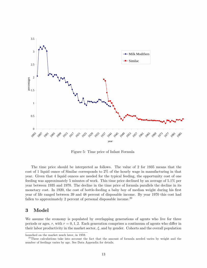
In Figure 5, we report the time price series for the �rst generation of milk modi�ers, Mellin�sand Nestle�s, in blue and the one for Similac in red. The �rst observation on Similac dates to 1935.While there was a large drop in the time price of the �rst generation of formulas before 1935, wefocus on Similac because it was the �rst commercially available formula to be deemed equivalentto mother�s milk and to became popular. In 1975, 52% of infants receiving commercially availablemilk-based formulas were fed Similac (see Table III in Fomon, 1975) and it remains very populartoday.19

15National Immunization Survey, CDC, 200316See http://www.slate.com/id/2138639/#ContinueArticle.17This information is available from ProQuest Historical Newspapers Chicago Tribune (1849-1985), Los Angeles

Times (1881-1985) and The Washington Post (1877 - 1990). We are grateful to Claudia Goldin for suggesting thisdata source. The details about the construction of the price series are discussed in the appendix.18Throughout the paper our measures of hourly wages is series Ba4361 from the Statistical Abstracts of the United

States: Bicentennial Edition (2006). Hourly wages (for full-time year-round workers) and prices are expressed in1982-1984 U.S. dollars (using the All Urban Consumers Consumer Price Index (CPI-U) as a de�ator.)19SMA did not achieve great popularity in the U.S, and in 1975 it accounted for less than 12% of the market

for commercially prepared formulas (Fomon, 1975). Alternative scienti�c infant formulas, such as Enfamil, were

11

0

10

20

30

40

50

60

70

80

90

100

1920 1925 1930 1935 1940 1945 1950 1955 1960 1965 1970

Year of Birth of Infant

Perc

enta

ge

Figure 4: Trends in breast-feeding

12

0

0.5

1

1.5

2

2.5

3

3.5

1893

1897

1901

1905

1909

1913

1917

1921

1925

1929

1933

1937

1941

1945

1949

1953

1957

1961

1965

1969

1973

1977

1981

1985

year

perc

enta

ges

Milk Modifiers

Similac

Figure 5: Time price of Infant Formula

The time price should be interpreted as follows. The value of 2 for 1935 means that thecost of 1 liquid ounce of Similac corresponds to 2% of the hourly wage in manufacturing in thatyear. Given that 4 liquid ounces are needed for the typical feeding, the opportunity cost of onefeeding was approximately 5 minutes of work. This time price declined by an average of 5.1% peryear between 1935 and 1970. The decline in the time price of formula parallels the decline in itsmonetary cost. In 1920, the cost of bottle-feeding a baby boy of median weight during his �rstyear of life ranged between 39 and 48 percent of disposable income. By year 1970 this cost hadfallen to approximately 2 percent of personal disposable income.20

3 Model

We assume the economy is populated by overlapping generations of agents who live for threeperiods or ages, r; with r = 0; 1; 2. Each generation comprises a continuum of agents who di¤er intheir labor productivity in the market sector, �; and by gender. Cohorts and the overall population

launched on the market much later, in 1959.20These calculations take into account the fact that the amount of formula needed varies by weight and the

number of feedings varies by age. See Data Appendix for details.

13

are split equally by gender and the distribution of labor market productivity is the same acrossgenders. In the �rst age of their life, all agents are single. They all marry in the second period oftheir life to an agent of di¤erent gender and with the same labor productivity and remain marriedin the third period. In each time period, t; a new generation of young agents is born, of the samesize. Hence, total population size is constant.

Agents value private consumption, c; and leisure, l; in all periods. Individual preferences canbe represented by the following lifetime utility function:

Xr=0;1;2

rYs=0

�s

!u (cr; lr) ;

where

u (c; l) =c1��

1� � + v (l) ;

and v (l) represents the sub-utility from leisure:

v (l) = 0l1�

1� ;

with �; 0; � 0. The parameters �r 2 (0; 1) represent the discount factor from age r to ager � 1: with �0 = 1: We allow for di¤erential discount factors to accommodate ages of di¤erentduration.

Leisure is de�ned as:l = T � h� p�n;

where T is the individual time endowment, p 2 [0; 1] denotes labor force participation, �n corre-sponds to the �xed number of work hours an employed individual works on the market, and hdenotes home hours.

Home hours are applied to the production of two home goods. The general household good,G; corresponds to activities such as meal preparation, cleaning, helping children with homework,vacation planning, yard work and other activities. This good must be produced at all ages of life.In the �rst period of marriage and only in that period, households must also produce the infantgood, I; which corresponds to activities deriving from the existence of infants in the household,such as pregnancy, childbirth and feeding. Hence, the �rst period of marriage can be interpretedas the fecund period of life:

The next section describes in detail the production technology for each home good.

3.1 Home Production

For each good, both time and market goods are inputs in production. The key assumption is thatwomen and men can equally contribute to the production of general household goods. Instead,only the wife�s time is used as an input in the production of infant goods. This asymmetry isclearly extreme, since the husbands�contribution to the production of infant goods is necessary,at least at conception. However, it provides a simple and realistic way of modelling women�scomparative advantage in the production of infant goods, based on the fact that only women cangive birth and breast feed.

The ratio of home hours to market goods in home production depends on technology. Thereare two technologies for the production of each home good, old and new. The new technologies are

14

less time intensive than the old. The old technologies are free, while there is a �xed cost to adoptthe new technologies expressed as a time price. This cost corresponds to the monetary value ofthe market goods associated with the new technologies translated into units of time. The timeprice of the new technologies can change over time. A decline in this price re�ects technologicalprogress embodied in the market goods used in production. Households choose which technologyto adopt for each home good in each period of their life.

3.1.1 Infant Goods

The infant goods are produced exclusively using the wife�s time. Their level of production isdenoted with I and does not vary with the technology, which only in�uences the time intensity ofproduction. Let hfI denotes the time required by the wife to produce I: Under the old technology:

I = minn�I�I ; h

fI (0)o; (1)

where hfI (0) = �I�I > 0: Under the new technology:

I = �1minn�I ; h

fI (1)o; (2)

with hfI (1) = �I > 0: The parameter �I > 1 represents the time saving associated with adoptionof the new technology, with hfI (0) = �I�I > hfI (1) = �I : The advantage of the new technologyis that it reduces the wife�s required time in the production of infant goods. The quantity �I�Iunder the new technology can be interpreted as the quantity of market goods associated withproduction, such as infant formula. The parameter �I corresponds to the time cost of pregnancy,childbirth and recovery and is present even if the new technology is adopted. The old technologyis free and we denote the price of the new technology with qI .

A few words of interpretation are in order here. The total time devoted by wives to infantgood production represents the sum of feeding time plus the time associated with pregnancy,childbirth and recovery. This is based on the notion that a pregnancy is associated with aphysical cost that reduces a woman�s ability to perform market work. The parameter �I measuresthis cost in equivalent time units. Based on the empirical evidence on the progress in medicineand obstetrics, most households were just confronted with �best� practices for behavior duringpregnancy, childbirth and recovery, while they chose how to feed their infants. Correspondingly,we treat the time cost of pregnancy, childbirth and recovery, �I ; as a parameter, and we modelbottle feeding as a choice. To incorporate the e¤ects of the reduction in the physical cost ofpregnancy over time re�ecting progress in medical knowledge and obstetric practices, as well aschanges in fertility, we will allow �I to vary over time with the measure of maternal mortality riskconstructed in section 2.

Under this interpretation, breast feeding is the only feeding method under the old technology,while under the new technology infants are fed formula with a bottle. Adoption of the newtechnology allows infant feeding, that under the old technology can solely be produced by themother, to become a general household good that could be produced by both spouses. Afterall, there is no di¤erence between bottle feeding an infant and general household goods, suchas helping children with homework or meal preparation, in terms of comparative advantage bygender. Hence, under the new I technology, the mother�s time required for infant feeding dropsto zero, a saving that corresponds to the parameter �I : On the other hand, the time requiredfor general good production rises by the amount �I (�I � 1) ; the time devoted to breast feeding.

15

Implicit in this treatment is the assumption that the time required for feeding does not dependon the method. Even under the new technology, the asymmetry in the spouses�contribution toinfant good production remains since mothers still have to bear the physical cost of pregnancy�I .

We now describe the production technology for general household goods.

3.1.2 General Household Goods

Our model for general household good production is similar to Greenwood, Seshadri, and Yoru-goklu (2005), henceforth GSY.

Let H��G�denote the contribution of home hours to production under technology �G = 0; 1;

where �G denotes whether the old (�G = 0) or the new (�G = 1) technology is used. Theproduction function for singles and old married households is:

G = min f�G�G;H (0)g ; (3)

G = �Gmin f�G;H (1)g :

The parameter �G > 1 denotes the time savings associated with the new G technology, so thatthe new technology requires fewer home hours, that is H (0) = �G�G > H (1) = �G: The quantity�G�G under the new technology can be interpreted as the quantity of market goods associatedwith the production of the general household good. We denote with qG the time price of the newhome durables technology, which re�ects the market value of the market goods associated withthe new G technology, such as home appliances, groceries etc. The old technology is free.

For married households, spouses contribute to the production of G according to:

H =

�0:5�hfG

��+ 0:5 (hm)�

�1=�; (4)

where the parameter � determines the substitutability of husbands�and wives�home hours in theproduction process. The spouses�contribution is symmetric; irrespective of the technology used.

For young married households, we incorporate the complementarity between infant and generalhousehold good production by letting the time requirement H vary with the technology adoptedfor producing the infant good, as described above. Speci�cally:

G�� I�= min

��G�G;H

�0; � I

�; (5)

G�� I�= �Gmin

��G;H

�1; � I

�;

where H�0; � I

�= �G�G+�

I�I (�I � 1) and H�1; � I

�= �G+�

I�I (�I � 1) ; and �I (�I � 1) is thetime required for infant feeding, an activity that becomes a general household good if the new Itechnology is adopted.21

We now describe the agents�optimization problems at each age in life.

21This is an analytically tractable way to model this complementarity, given our technological assumption. Ofcourse, since the choice of technology does not e¤ect the level of production or utility directly, many other strategieswould be equivalent.

16

3.2 Single Agents�Problem

Agents are born with no wealth and cannot borrow against future income. At age 0; they aresingle. They decide on whether to participate in the labor force in that period, on whether toacquire market skills, on how to produce the home good G and on how much to save. Theacquisition of market skills has a time cost of > 0 and a¤ects their labor market productivityat ages r = 1; 2; as follows:

�j = ��1 + "ej

�; (6)

where the parameter " represents the returns to skills and ej = 0 when no skills are acquired andej = 1 otherwise.

A single individual�s problem is:

�j0 (�) = maxaj1�0;p;e2f0;1g;�G

u�c; T � e � h

��G�� p�n

�+ �1�

j1

�aj1; e; �

�; (Problem S)

subject to (6), (3) and:c+ aj1 � w

��p� �GqG

�;

for j = f;m: Here, �j1�aj1; e; �

�denotes the maximized present discounted value of individual

lifetime utility at the beginning of period 1; which will be derived below. The variable w de-notes economy-wide real wages in e¢ ciency units of labor and may change over time, due toimprovements in the market production technology.22

3.3 Household Problem

We model married individuals according to Chiappori�s (1988, 1997) collective labor supply ap-proach. Under this paradigm, household decisions are Pareto e¢ cient. Households choose asequence of private consumption, participation, and home hours for each spouse, as well as tech-nologies for the production of the home goods, subject to an intertemporal budget constraint andto the technological and feasibility constraints.23

We �rst describe the optimal choice of home hours in each period, taking as given the pro-duction technology. This step amounts to solving the following cost minimization problem:

C��H; �hfI

�= min

hm2[0;�h];hfG2[0;�h�hfI ]��1 + "ef

�hf + � (1 + "em)hm

subject tohf = hfI + hfG;�

0:5 (hm)� + 0:5�hfG

���1=�� �H;

22We assume that progress in market technology is not gender biased and that the distribution of individual pro-ductivities, which is symmetric across genders, remains constant over time. For an analysis of skill bias technologicalchange and its e¤ects on female participation and fertility, see Galor and Weil (1996).23The Pareto problem can be decentralized by allowing each spouses to individually choose labor force participa-

tion and private consumption in each period. Households then jointly choose a rule for sharing household wealth,savings, the allocation of home hours and the technologies for producing the home goods. The fact that saving is ajoint household decision implies that individual problems are static. Moreover, the household is implicitely assumedto have commitment in the joint choices.

17

hfI � �hfI ;

for some �H = H��G; � I

�and �hfI = hfI

�� I�:

The �rst order necessary conditions for hfG and hm for interior solutions are:

��1 + "ef

�(hfG)

��1 =� (1 + "em)

(hm)��1; (7)

�0:5 (hm)� + 0:5

�hfG

���1=�= �H;

hfI = �hfI :

We will denote with hj��G; � I

�for j = f;m the policy functions for the cost minimization

problem. By (7), if ef = em, then, the solution is hfG = hm: If instead ef � em; then, the onlysolution has hfG > hm: Hence, the symmetry in the spousal allocation of home hours devote tothe production of G depends on the opportunity cost of home hours, that is potential wages, foreach spouse.

Let Zt denote total household expenditures net of total household income in period t: Then:

Z��G; � I ; qG; qI ; w

�=

Xj=f;m

�cj + �jlj

�+ w

hC�H��G�; hfI

�� I��+ qG�G + qI� I

i�Tw

Xj=f;m

�j :

Substituting in the expressions for the cost of production of the two public goods, we obtain:

Z��G; � I ; qG; qI ; w

�=Xj=f;m

cj + w�qG�G + qI� I

�� w

Xj=f;m

�jpj�n;

where w corresponds to the contemporaneous value of economy-wide real wages. Hence, thehousehold�s intertemporal budget constraint is given by:

Z1��G1 ; �

I1; q

G1 ; q

I1 ; w1

�+Z2��G2 ; �

I2; q

G2 ; q

I2 ; w2

�1 +R2

� a1; (8)

where a1 is household wealth at the beginning of age 124: The households initial wealth a1 is given

by the sum of the spouses�wealth at the beginning of age 1; a1 =�af1 + a

m1

�(1 +R1) ; where the

values of aj1 solve the spouses�individual optimization problem when single.The households�Pareto problem is given by:

max�I1;fcjr;pjr;�Gr gr=1;2;j=f;m

Xr=1;2

�r�12

Xj=f;m

�ju�cjr; T � hjr

��Gr ; �

Ir

�� pjr�n

�subject to (8) and (3), (1)-(2), (6), with ejr = 0 for r = 1; 2; h

fI2 = 0 and hf2 = hfG2 and where �j

j = f;m denote the spouses�Pareto weights.

24Here, the home goods are not marketable, so their production level does not enter in the household budgetconstraint. See Chiappori (1997) for a discussion.

18

Since at age 2 the infant good is not produced, and � I2 = 0 and hfI2 = 0; so that hf2 = hfG2 :

Given the lumpy nature of the choice of �Gr and �I1; and the fact that home hours are determined

by the cost minimization problem as a function of technology, the only �rst order necessaryconditions for the household problem are:

�jujc;1 � � = 0; for j = f;m; (9)

�j�2ujc;2 � � (1 +R2) = 0; for j = f;m; (10)

�jujl;1 � �w1e

j = 0; for j = f;m; (11)

�j�2ujl;2 � � (1 +R2)w2e

j = 0; for j = f;m; (12)

for given values of �Gr and �I1; as well as the intertemporal budget constraint (8). Here, � is the

multiplier on the intertemporal budget constraint:The intertemporal pattern of consumption is independent from the distribution of the Pareto

weights or the choice of technology and labor force participation patterns over time. Instead, thehigher the Pareto weight of a spouse, the higher the optimal level of consumption and leisure. Itfollows that pjr is decreasing in �j coeteris paribus, so that wives will participate more if theirPareto weight is lower.

The Euler equation for the individual saving choice at age 0 is:

�u0�pj0� � a

j1; T � e

j0 � p

j0�n�+ �1�

j1;a

�aj1; e; �

�� � 0;= 0 for aj1 > 0:

(13)

The envelope condition for this problem is:

�j1;a

�aj1; e; �

�=

�

�j; for j = f;m: (14)

Intuitively, a spouse with a higher Pareto weight will obtain a larger share of resources whenmarried and �nds it optimal to bring lower wealth levels into the marriage, other things equal.

Here, as previously noted, �j1�aj1; e; �

�is the maximized present discounted value of lifetime

utility at the beginning of period 1: Given that this corresponds to the individual value functionfor the household�s optimization problem, it is possible to incorporate the agent�s problem whensingle into the household problem, to simplify the derivation of lifetime consumption, home hoursand participation paths. We describe this strategy of solving the household problem in detail inthe Model Appendix.

3.4 Market Production and Equilibrium

A continuum of identical, perfectly competitive �rms in each period produce an undi¤erentiatedoutput using labor only, and then convert it into consumption goods and goods used in theproduction of general household and infant goods.

The representative �rm produces the undi¤erentiated output, Y; according to the productionfunction:

Y � �N; (15)

19

where the variable Y denotes per capita production of the undi¤erentiated good and N is percapita (average) labor input in e¢ ciency units, given by:

N =

Zip (i) �i (1 + ei) d� (i) ; (16)

where i indexes individuals in the population. Here, � corresponds to average labor productivity.� may grow over time to re�ect technological advancements in market production. Y can betransformed into home durables, D; commodities used in the production of infant goods K; andprivate consumption goods, C; according to the technology:

GD + IK + C � Y: (17)

Given that all technologies are constant returns to scale and that the production sector iscompetitive, w = � in equilibrium, so that wages will grow one to one with market productivity.In addition, competitive pricing pins down the equilibrium values of ql as a function of thetechnological marginal rates of transformation l; for l = G; I.

We describe the representative �rm�s problem and the derivation of the equilibrium in theModel Appendix.

4 Quantitative Analysis

We calibrate parameters to match the equilibrium of our model to a variety of data statistics in1920. We then simulate the transition between 1920 and 1970 predicted by the model, by feedingin measures of technological progress in general and infant good technologies, as well as the risein economywide real wages over this period. Finally, we run several experiments to gauge thecontribution of the introduction of each source of technological progress in isolation.

4.1 Calibration

We set �f = �m = 0:5 so that spouses have equal bargaining power: We �x � = 1 and = 1;so that utility is logarithmic in private and public consumption. This implies that wealth andsubstitution e¤ects of changing new technology prices and aggregate wages exactly cancel. Weinterpret the single period as covering ages 15-22, and the second period as covering ages 23-35.We consider the last period as corresponding to ages 36-60. We set the yearly interest rate at 5%,and �x �1 = exp(�0:05 � 7) and �2 = exp (�0:05 � 13) ; with Rr = 1=�r � 1 for r = 1; 2:

We calibrate the remaining parameters to match certain data statistics of interest in 1920.We parameterize the G technology as follows. Given our assumption that spouses have a

symmetric role in the production of G; we allow for high substitutability between home hours ofwives and husbands, and we set � = 0:9: This corresponds to an elasticity of substitution betweenhusbands�and wives�home hours in the production of G equal to 10:0. We set the parameters�G and �G based on the assumption that all households in which the wife participates in thelabor force adopt the new technologies in 1920. Using the value of home hours of married women,

20

conditional on participation in the labor force, and of married men in 1920, this delivers:

�G�G =

"0:5 �

�4

112

��+ 0:5

�51

112

��#1=�= 0:2346;

�G =

"0:5 �

�4

112

��+ 0:5

�25

112

��#1=�= 0:1256;

which implies �G = 1:87.For the infant good technology, recall that the parameter �I to corresponds to the time cost

of pregnancy, childbirth and recovery as a fraction of the time endowment, while the parameter�I to correspond to the time saving associated with bottle feeding relative to breast-feeding.

We use our estimate for the number of pregnancies, P �; based on the calculations describedin Section 2 to obtain a value for �I , under the assumption that for each pregnancy, womenexperience 4.5 unproductive months. Then, as a fraction of their time endowment during theyoung married period, this component of the cost is equal to:

�I (1920)=P �1920 � (4:5=12)

35� 23 :

To compute the time cost associated with infant feeding, we use infant feeding charts from theNational Association of Pediatrics, according to which the average time required to breast-feedone child for the �rst 12 months ranges between 14 and 17.30 hours per week 25 Given the adjustedcompleted fertility rate, TFR�, the fraction of the time endowment that women spent nursing isTFR�1920�(17=112)

35�23 : The total time commitment then adds to:

�I (1920) =�I (1920) + TFR

�1920 � (17=112) = (35� 23)�I (1920)

:

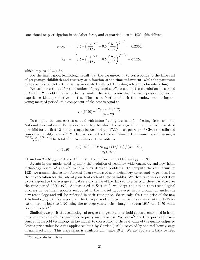
�Based on TFR�1920 = 3:4 and P� = 3:6; this implies �I = 0:1141 and �I = 1:35:

Agents in our model need to know the evolution of economy-wide wages, w; and new hometechnology prices, qI and qG; to solve their decision problems. To compute the equilibrium in1920, we assume that agents forecast future values of new technology prices and wages based ontheir expectation for the rate of growth of each of these variables. We then take this expectationto correspond to the average annual rate of change of the data counterparts of these variable overthe time period 1920-1970. As discussed in Section 2, we adopt the notion that technologicalprogress in the infant good is embodied in the market goods used in its production under thenew technology and will be re�ected in their time price. So we take the time price of the newI technology, qI ; to correspond to the time price of Similac. Since this series starts in 1935 weextrapolate it back to 1920 using the average yearly price change between 1935 and 1970 whichis equal to 5.08%.

Similarly, we posit that technological progress in general household goods is embodied in homedurables and we use their time price to proxy such progress. We take qG; the time price of the newgeneral household technology in the model, to correspond to the real value of the quality-adjustedDivisia price index for eight appliances built by Gordon (1990), rescaled by the real hourly wagein manufacturing. This price series is available only since 1947. We extrapolate it back to 1920

25See appendix for details.

21

applying to home durables the methodology developed by Cummins and Violante (2002).26 Theaverage yearly rate of decline in this variable is 4.6%.

We calibrate the relative price of the new home technologies, the ratio qI=qG; using informationon the monetary cost of formula and on historical prices for home appliances 1920. We assumethat a household who adopts the new G technology purchases a refrigerator, a washer and avacuum cleaner and that the appliances need to be replaced every 5 years. Thus, a householdmust replace them twice in the young married period. The replacement cost corresponds totheir price in the year of replacement, computed using the series for the price of home durables.Similarly, we convert the cost of feeding one child with infant formula to 1920 dollars. The ratioof the cost of feeding one child with infant formula and the cost of buying the three major homeappliances in 1920 is 0:084: We then multiply this ratio by the total fertility rate in 1920, whichis equal to 3:26: This delivers: qI=qG = 0:27:

We assume the distribution of � is log-normal, with mean �� and standard deviation ��. Thisleaves six remaining parameters: qG; "; ; 0; �� and ��: which we calibrate to match the value in1920 of the following population statistics: home hours of married women who participate in thelabor force, home hours of married women who do not participate in the labor force, home hoursof men, the average rate of adoption of new general household technologies, the average rate ofbottle feeding, and labor force participation of married women by cohort as a ratio to the laborforce participation of men. Speci�cally, our target for the labor force participation of old marriedwomen in our model is the labor force participation rate in 1920 of white married women bornbetween 1866 and 1885 over the labor force participation of men in 1920. Our target for the laborforce participation of young married women in our model corresponds to the participation rate in1920 of white married women born between 1886 and 1895 over the labor force participation ofmen in 1920. We select the parameterization that minimizes the sum of squares of the distance ofthe values predicted by our model for those parameters and the corresponding data statistic. Thepopulation statistics and the corresponding model values are listed in Table 3. The calibratedparameters are reported in Table 4.

Table 3: Calibration Targets

Population Statistic Value in 1920 Model ValueHome hours of married women who do not participate in the labor force 51 49Home hours of married women who participate in the labor force 25 22Male home hours 4 7Average adoption of new general household technology 7% 8%Average adoption of bottle feeding technology 15% 15%Labor force participation of young married women 9% 9%Labor force participation of old married women 6.5% 6.5%

The data on labor force participation of married women by cohort in 1920 is reported inGoldin (1990). The 1920 targets for home hours by gender and employment status of wives aredescribed in the Data Appendix. In order to obtain the targets in model units, we simply dividethe 1930s statistics for home hours per week by 112, the non-sleeping hours per week. We rescalethe home hours targets in model units, based on 112 non-sleeping hours per week and a 40 hour

26Details about the construction of the price series for home durables are in the appendix.

22

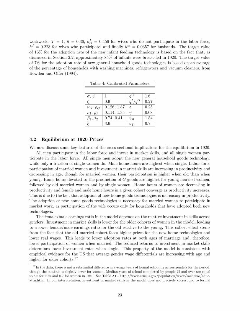
workweek: T = 1; �n = 0:36; hfG = 0:456 for wives who do not participate in the labor force,hf = 0:223 for wives who participate, and �nally hm = 0:0357 for husbands. The target valueof 15% for the adoption rate of the new infant feeding technology is based on the fact that, asdiscussed in Section 2.2, approximately 85% of infants were breast-fed in 1920. The target valueof 7% for the adoption rate of new general household goods technologies is based on an averageof the percentage of households with washing machines, refrigerators and vacuum cleaners, fromBowden and O¤er (1994).

Table 4: Calibrated Parameters

�; 1 qG 1.6� 0.9 qI=qG 0.27�G; �G 0.126, 1.87 " 0.25�I ; �I 0.114, 1.35 0.08�1; �2 0.74, 0.41 0 1.54�� 3:6 �� 0:7

4.2 Equilibrium at 1920 Prices

We now discuss some key features of the cross-sectional implications for the equilibrium in 1920.All men participate in the labor force and invest in market skills, and all single women par-

ticipate in the labor force. All single men adopt the new general household goods technology,while only a fraction of single women do. Male home hours are highest when single. Labor forceparticipation of married women and investment in market skills are increasing in productivity anddecreasing in age, though for married women, their participation is higher when old than whenyoung. Home hours devoted to the production of G goods are highest for young married women,followed by old married women and by single women. Home hours of women are decreasing inproductivity and female and male home hours in a given cohort converge as productivity increases.This is due to the fact that adoption of new home goods technologies is increasing in productivity.The adoption of new home goods technologies is necessary for married women to participate inmarket work, as participation of the wife occurs only for households that have adopted both newtechnologies.

The female/male earnings ratio in the model depends on the relative investment in skills acrossgenders. Investment in market skills is lower for the older cohorts of women in the model, leadingto a lower female/male earnings ratio for the old relative to the young. This cohort e¤ect stemsfrom the fact that the old married cohort faces higher prices for the new home technologies andlower real wages. This leads to lower adoption rates at both ages of marriage and, therefore,lower participation of women when married. The reduced returns to investment in market skillsdetermines lower investment rates when single. This property of the model is consistent withempirical evidence for the US that average gender wage di¤erentials are increasing with age andhigher for older cohorts.27

27 In the data, there is not a substantial di¤erence in average years of formal schooling across genders for the period,though the statistic is slightly lower for women. Median years of school completed by people 25 and over are equalto 8.6 for men and 8.7 for women in 1940. See Table A1 - http://www.census.gov/population/www/socdemo/educ-attn.html. In our interpretation, investment in market skills in the model does not precisely correspond to formal

23

The model predicts higher home hours for men with working wives relative to the data. Thisis due to the fact that more married women who participate in the labor force in the model haveinvested in market skills than in data. Since they have the same wage as their husbands, theallocation of home hours is symmetric in those households in the old period.

4.3 Transition

Our model features four exogenous sources of technological change. The �rst is the increase ineconomy wide labor productivity, due to technological progress in market good production, re-�ected in the average real wage. The second is the improvement in general household technologiesas re�ected in the decline in the time price of these technologies. These factors in�uence the op-portunity cost of home production for both genders. Third, the introduction of time-saving infantfeeding technologies and their improvement over time, re�ected in the decline in the time priceof breast-milk substitutes. Lastly, a reduction in the time cost of pregnancy driven by improvedmedical practices and knowledge leading to lower maternal mortality rates, as well as by changesin fertility. The third and fourth factor have a direct impact on women only.

To evaluate the role of these factors, we use measures of these variables for the time period andfeed them into the model to examine the properties of the transition between 1920 and 1970. Foreconomy wide labor productivity we use real wages. For the new general household technology weuse Gordon�s Divisia price index as described in Section 4.1. For the new infant good technologywe use the time price of Similac. Finally, we estimate the variation over time in the time cost ofpregnancy and in the time savings associated with formula feeding following the strategy describedin Section 2.

We use the maternal risk as a proxy for the decline in the time cost of pregnancy, childbirthand recovery associated with the medical advancements we discussed in section 2. We set:

�I (t) =M ~Mt � �I (1920) ;

�I (t) = 1 +TFR�t � (17=112)(33� 23) �I (t)

;

where M ~Mt = MatMortt=MatMort1920; and MatMortt is the maternal mortality rate at timet: We index of technological progress then corresponds to the variable M ~Mt.

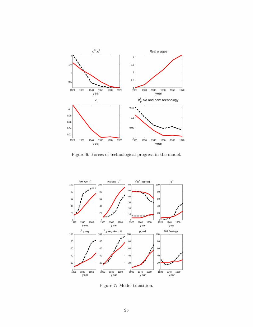
Figure 6 plots the transitional forces at work in our model over the period of interest. Wesimulate the transition in our model and run several experiments to evaluate the impact of eachforce in isolation. Consistent with our calibration strategy, we assume that agents forecast thechange in new technology prices and real wages over their lifetime using the yearly average changeover the period of interest. Our results for the transition are displayed in �gure 7, where the solidred lines correspond to data and the dashed black lines correspond to model predictions.

The model over predicts the rise in the labor force participation of young married women andin the adoption of the new infant good technology. By 1970, 83% of all young married womenparticipate in the labor force when young (dashed-line in panel 5), and 90% of young marriedhouseholds adopt the new infant good technology (panel 1), whereas in the data only 47% of

schooling, but to e¤ort exerted in early labor market experiences that may in�uence future carrier paths and earningpotential.

24

1920 1930 1940 1950 1960 1970

0.5

1

1.5

2

year

qG,qI

1920 1930 1940 1950 1960 19701

1.5

2

2.5

3

year

Real w ages

1920 1930 1940 1950 1960 1970

0.02

0.04

0.06

0.08

0.1

year

νI

1920 1930 1940 1950 1960 19700

0.05

0.1

0.15

year

hfI, old and new  technology

Figure 6: Forces of technological progress in the model.

1920 1940 19600

20

40

60

80

100

y ear

Average τI

1920 1940 19600

20

40

60

80

100

y ear

Average τG

1920 1940 19600

10

20

30

40

50

60

y ear

hf,hm, married

1920 1940 19600

20

40

60

80

100

y ear

ef

1920 1940 19600

20

40

60

80

100

y ear

pf, young

1920 1940 19600

20

40

60

80

100

y ear

pf, young when old

1920 1940 19600

20

40

60

80

100

y ear

pf, old

1920 1940 19600

20

40

60

80

100

y ear

F/M Earnings

Figure 7: Model transition.

25

young married women participate and the formula feeding rate is 75%.28 This outcome is due tothe fact that the decline in qI is very rapid between 1920 and 1950. The adoption of the new Gtechnology is slightly slower than in the data. The slow adoption of the new general householdtechnologies in the model re�ects that fact that until 1940 there is no signi�cant reduction in itstime price. Households in the model substitute by increasing the adoption of new infant goodtechnologies at a very fast rate.

The ability to invest in market skills ampli�es the e¤ect of the new home technologies onwomen�s labor force participation and accelerates the transition in the model. We plot the fractionof married women that have invested in market skills in each year in panel 4. In 1920, this fractionis equal to 3%, it then declines to 1% in 1930, re�ecting the higher fertility rates single womenin that cohort, and it takes o¤ in 1940 rising to 45% in 1970. We interpret this variable broadly,re�ecting not only years of formal education but also additional time invested in their careers thatworkers can only pursue early in their employment history. This implies that there is no singlesummary measure of this variable that we can use to compare the model�s prediction with the dataalong this dimension. In �gure 7, we compare women�s investment in market skills in the modelwith the percentage of white women graduating from college by cohort29. The college graduationrates average 6% in 1920 and rise to 25% in 1970. Interestingly, the take o¤ for women�s collegegraduation rates in the data occurs in 1940, as predicted by our model.

We report the female/male ratio of average labor earnings in panel 8 (dashed line) and wecompare it to the ratio of wage income for the white married population from the Census. Themodel predicted value of 20% for 1920 is very close the its empirical counterpart, equal to 21%.The earnings ratio drops in the model in 1930 and 1940, to 13 and 14%, respectively. This ismainly a compositional e¤ect, due to the entry of unskilled married women in the labor force inthat time period, which determines a decline of average wage income of women, conditional onparticipation. The earnings ratio rises steadily from 1950 onward in the model, reaching 50% in1970, whereas in the data it is only 28% at the same date.

Labor force participation of married women increases with age in the model, consistent withthe data. This can be seen from panels 5 and 6, where the dashed-dotted line corresponds tothe labor force participation rate of young married women when old. The value predicted by ourmodel is quite close to the data until 1940 after which it rises at a faster rate than in the data.This outcome is driven by the acceleration in women�s investment in market skills in 1940, whichis more intense in the model than in the data, as well as by the fast adoption of new infant goodtechnologies in 1930.

The rates of participation for old married women is very close to the data. In all years, young

28We compute period average by cohort in the model simulations. This is required since the young married periodlasts 11 years, the old married period lasts 27 years, which is longer than the 10 year time interval we adopt for oursimulations. Hence, when we compute the transition, 1/11 agents that were young in 1920 will still be young in1930. Similarly, 7/27 agents that were old married in 1920 will still be old married in 1940, 10/27 will still be oldmarried in 1930. To take this into account in the transition, we treat 1920 as if everybody is a new single agent, anew young married agent and a new old agent, consistent with our calibration. In 1930 we compute all the decisionsfor the new single, young married and old married agents. The population statistics on the young married and oldmarried that we report for 1930 re�ect the fact that 10/11 young marrieds in 1930 are new young marrieds and1/11 young marrieds made their decisions in 1920 and behave accordingly. Similarly for the old married agents andfor all successive years.This treatment is consistent with the maintained assumption that at each stage in life agents make all their

decision at the beginning of the period based on the current prices/wages and expected future prices.29Source: U.S. Bureau of the Census, Current Population Reports, Series P-20, Educational Attainment in the

United States.

26

married women (dashed line in panel 5) exhibit higher participation rates than old married women(panel 7). This cohort e¤ect, which is also present in the data, is due to the fact that old marriedwomen face lower lifetime earnings due to rising real wages and higher new home technologyprices. This reduces their incentive to invest in market skills and their opportunity cost of homeproduction relative to men.

Finally, home hours of married women decline signi�cantly, while male home hours increaseover time. This outcome is mostly driven by the rising rates of women�s investment in marketskills at all ages, which induces greater symmetry in the household allocation of home hours. Totalleisure for married men then decreases substantially relative to total leisure of married womenwho participate in the labor force. Home and market work for participating married women,excluding the time devoted to the production of infant goods, totals to 65 hours in 1920, and fallsto 54 hours in 1970. For married men, total work amounts to 48 hours in 1920 and rises to 53hours in 1970 in the model.

This prediction is consistent with empirical evidence for the US, on the decline in leisuretime for men married to women who participate in the labor force relative to their wives. Thisphenomenon is discussed by Knowles (2005), who focusses on the time period 1965-2003. Forour period of interest, it is not possible to measure home hours of husbands conditional on theparticipation status of their wife. However, the downward trend in married men�s leisure relativeto their wife is clearly present. Knowles (2005) argues that the decline in married men�s relativeleisure is due to an increase of wives� bargaining power within the household. In our model,this outcome stems from the fact that women�s lower comparative advantage in home productionincreases wives�earning potential on the labor market and induces a more equal distribution ofhome hours.

4.3.1 Discussion

How do we interpret the fact that the model largely overpredicts the labor force participationof young married women and the rate of adoption of new infant good technologies relative tothe data? The evolution of household technologies and labor productivity is the only force thatin�uences female labor force participation and gender earnings di¤erentials in the model, whileother factors may also play a role and dampen the e¤ect of improving technologies in practice.

One very important factor which we abstract from is the presence of �marriage bars� forwomen until the 1950�s. Marriage bars consisted in the practice of not hiring married women ordismissing female employees when they married. Marriage bars were prevalent in teaching andclerical work, which accounted for approximately 50% of single women�s employment between 1920and 1950. Goldin (1991) extensively documents the pervasiveness of these practices for di¤erentschool districts and for �rms hiring o¢ ce workers. The probability of not retaining single femaleworker upon marriage ranged between 47.5% to 58.4% for school districts between 1928 and 1942,and between 25% and 46% for �rms hiring o¢ ce workers between 1931 and 1940. The probabilityof not hiring a married woman ranged between 62% and 78% for school districts and between39% and 61% for �rms hiring o¢ ce workers over the same periods.

Conditional on employment, di¤erences in wages across genders are purely driven by di¤er-ences in investment in market skills in our model. We do not allow for statistical or taste baseddiscrimination. Yet, even in current years approximately 10% of the gender di¤erences in earningscannot be accounted for by observable di¤erences in characteristics that are related to produc-tivity (O�Neill, 2000). Albanesi and Olivetti (2006) argue that this unexplained gender earnings

27

di¤erential could be due to statistical discrimination. Gender discrimination would greatly reducewomen�s incentive to invest in market skills and participate in the labor force in our model.30

Cultural factors may also have played an important role in slowing down the increase inwomen�s labor force participation. Fernández and Fogli (2005) document the strong role ofcountry of origin, a proxy for cultural di¤erences in attitudes with respect to women�s work,in second-generation American women�s labor force participation behavior. Based on survey ev-idence reported in Fogli and Veldkamp (2007) and Fernández (2007), only 20% of respondentsbelieved that a married woman should work in the period between 1935 and 1945. By 1970, thisnumber went up to 55%, a very signi�cant rise to a level that still suggests a signi�cant culturalbarrier to women�s employment.31

We also assume that the distribution of bargaining power in the household is exogenous, con-stant over time and equal across spouses. Empirical evidence32 suggests that the distribution ofbargaining power across spouses depends on relative wages. Based on this, the assumption thatspouses have symmetric bargaining power in the 1920�s seems unrealistic since married women hadlower earning potential. Institutional factors, such as divorce laws, lack of political representationand marriage bars in the labor market may also have contributed to reduce women�s bargainingpower in the household. The gradual lifting of these constraints over the course of the twentiethcentury can be represented as an increase of the wives�Pareto weight in the household problemin the context of our model. Knowles (2005) argues that the reduction in female/male earningsdi¤erential indeed increased the bargaining power of women and led to a decline in gender di¤er-entials in home hours. In our model, a rising Pareto weight for married women would lead to aslower increase in their participation, since this is inversely related to their Pareto weight in thehousehold problem.

Lastly, we assume that the only cost associated to the adoption of new infant good technology isthe monetary cost and that infant formula was readily available in all locations after its commercialintroduction. In practice, there could be additional learning costs associated with the use of infantformula that slow down its di¤usion in the population or uncertainty about the e¤ectiveness offormula as a substitute for mother�s milk. For example, formula was initially not available in alllocations. In the 1920s and early 1930s, di¤usion of knowledge on infant formula mainly occurredvia women giving birth in hospitals. For this period, the rate of hospital birth can in fact beconsidered an upper bound on the possible rate of di¤usion of infant formula. In addition, asdiscussed in Section 2, in the early 1970s, new scienti�c discoveries regarding the positive e¤ect ofmother�s milk on the immune status of the baby and on the child�s resistance to infections broughtabout a resurgence in breast feeding. The inclusion of additional adoption costs for infant formula,as well as constraints on di¤usion, would dampen the adoption rate of infant formula in the modeland slow down the rise in married women�s labor force participation.33

30Numerical experiments suggest that di¤erential returns to work or skill investment by gender do not signi�cantlya¤ect the transition. This is due to the fact that the conventional measures of these gender di¤erentials do not varymuch over this time period.31Fogli and Veldkamp (2007) and Fernández (2007) point to uncertainty about the e¤ect of mother�s work on the

welfare of young children as an important determinant of these attitudes.32See Browning, Bourguignon, Chiappori, and Lechene (1994) and Mazzocco (2007).33The new discoveries on the immunization properties of mother�s milk could be modelled as a negative shock to

the productivity of the new infant good technology. That is, adopting the new technology, would still save time butdeliver a lower quantity of infant good. If preferences were de�ned over the quantity of infant goods, this wouldlead, other things equal, to higher breast feeding rates.

28

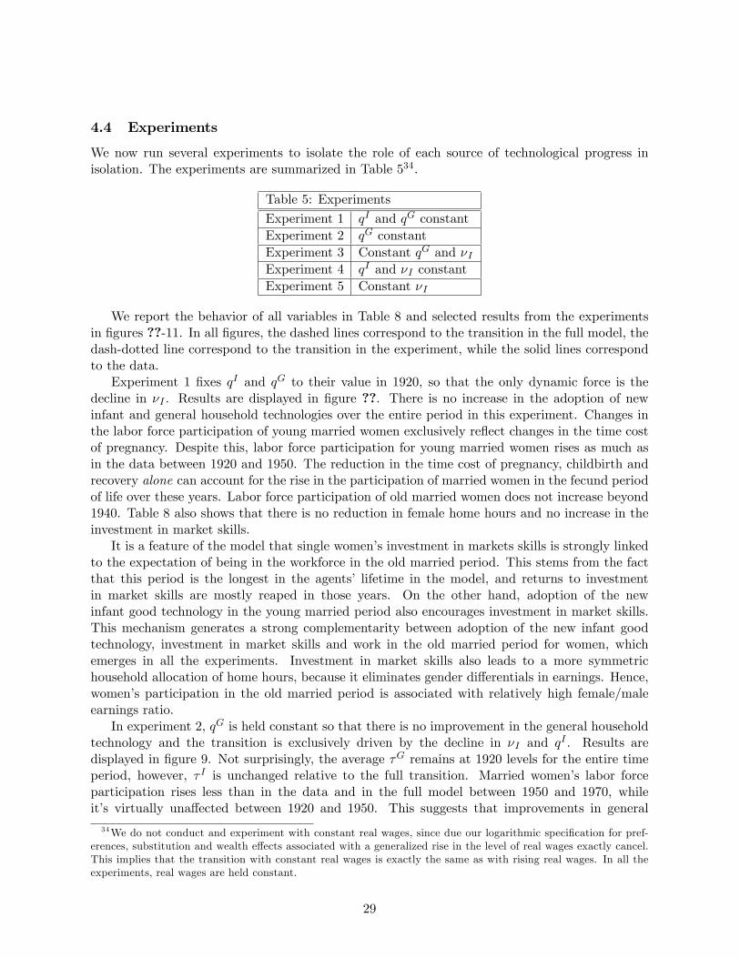
4.4 Experiments

We now run several experiments to isolate the role of each source of technological progress inisolation. The experiments are summarized in Table 534.

Table 5: Experiments

Experiment 1 qI and qG constantExperiment 2 qG constantExperiment 3 Constant qG and �IExperiment 4 qI and �I constantExperiment 5 Constant �I

We report the behavior of all variables in Table 8 and selected results from the experimentsin �gures ??-11. In all �gures, the dashed lines correspond to the transition in the full model, thedash-dotted line correspond to the transition in the experiment, while the solid lines correspondto the data.

Experiment 1 �xes qI and qG to their value in 1920, so that the only dynamic force is thedecline in �I . Results are displayed in �gure ??. There is no increase in the adoption of newinfant and general household technologies over the entire period in this experiment. Changes inthe labor force participation of young married women exclusively re�ect changes in the time costof pregnancy. Despite this, labor force participation for young married women rises as much asin the data between 1920 and 1950. The reduction in the time cost of pregnancy, childbirth andrecovery alone can account for the rise in the participation of married women in the fecund periodof life over these years. Labor force participation of old married women does not increase beyond1940. Table 8 also shows that there is no reduction in female home hours and no increase in theinvestment in market skills.

It is a feature of the model that single women�s investment in markets skills is strongly linkedto the expectation of being in the workforce in the old married period. This stems from the factthat this period is the longest in the agents� lifetime in the model, and returns to investmentin market skills are mostly reaped in those years. On the other hand, adoption of the newinfant good technology in the young married period also encourages investment in market skills.This mechanism generates a strong complementarity between adoption of the new infant goodtechnology, investment in market skills and work in the old married period for women, whichemerges in all the experiments. Investment in market skills also leads to a more symmetrichousehold allocation of home hours, because it eliminates gender di¤erentials in earnings. Hence,women�s participation in the old married period is associated with relatively high female/maleearnings ratio.

In experiment 2, qG is held constant so that there is no improvement in the general householdtechnology and the transition is exclusively driven by the decline in �I and qI . Results aredisplayed in �gure 9. Not surprisingly, the average �G remains at 1920 levels for the entire timeperiod, however, � I is unchanged relative to the full transition. Married women�s labor forceparticipation rises less than in the data and in the full model between 1950 and 1970, whileit�s virtually una¤ected between 1920 and 1950. This suggests that improvements in general

34We do not conduct and experiment with constant real wages, since due our logarithmic speci�cation for pref-erences, substitution and wealth e¤ects associated with a generalized rise in the level of real wages exactly cancel.This implies that the transition with constant real wages is exactly the same as with rising real wages. In all theexperiments, real wages are held constant.

29

1920 1930 1940 1950 1960 19700

20

40

60

80

100

y ear

Av erage τI

1920 1930 1940 1950 1960 19700

20

40

60

80

100

y ear

Av erage τG

1920 1930 1940 1950 1960 19700

20

40

60

80

100

y ear

LFP, old married women

1920 1930 1940 1950 1960 19700

20

40

60

80

100

y ear

LFP, y oung married women

Figure 8: Experiment 1

household technologies play a strong role in the later time period. In the early period, risingfemale participation rates are mostly driven by young married women entering the labor forceas �I declines and households adopt the new infant good technology, and this pattern is mostlyuna¤ected by the constant value of qG: The high value of qG has a direct negative e¤ect onparticipation of old married women. This discourages investment in market skills and indirectlyalso a¤ects young married women�s participation in the labor force between 1950 and 1970, despitethe high rates of adoption of new infant good technologies.

We report the results for experiment 3 in Table 8. This experiment isolates the e¤ect of adecline in qI since both �I and qG are constant. Labor force participation of young marriedwomen rises from 9% in 1920 to 20% in 1970. This suggests that the declining cost of infantformula alone can account for only a small fraction of the rise in participation of young marriedwomen, and the decline in the time cost of pregnancy, childbirth and recovery instead has a muchstronger impact over those years.

Experiment 4 isolates the e¤ect of the decline in qG: The results are displayed in �gure 10.With qI and �I constant, � I is also constant. The labor force participation of young marriedwomen is lower than in the full transition and much lower than in the data between 1920 and1950. Absent any decline in qI or �I ; young married women�s labor force participation is 9%lower than in the data in 1930, 13% lower in 1940, 3% lower in 1950. This suggests that in themodel the rise in the labor force participation of young married women is strongly driven byprogress in medical technologies. By contrast, old married women�s labor force participation andthe adoption of new general household technologies are virtually una¤ected with respect to themodel with all sources of technological progress. As reported in Table 8, investment in marketskills is lower in 1960 and 1970, which depresses the F/M earnings ratio for that period.

30

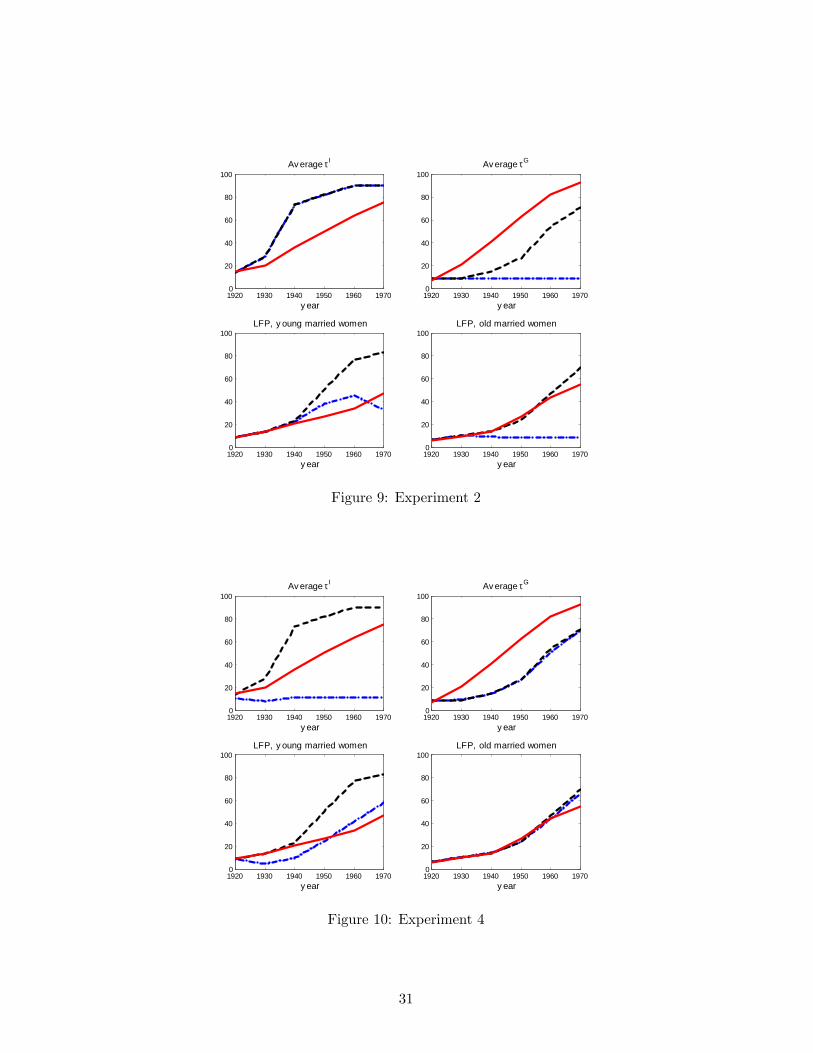
1920 1930 1940 1950 1960 19700

20

40

60

80

100

y ear

Av erage τI

1920 1930 1940 1950 1960 19700

20

40

60

80

100

y ear

Av erage τG

1920 1930 1940 1950 1960 19700

20

40

60

80

100

y ear

LFP, old married women

1920 1930 1940 1950 1960 19700

20

40

60

80

100

y ear

LFP, y oung married women

Figure 9: Experiment 2

1920 1930 1940 1950 1960 19700

20

40

60

80

100

y ear

Av erage τI

1920 1930 1940 1950 1960 19700

20

40

60

80

100

y ear

Av erage τG

1920 1930 1940 1950 1960 19700

20

40

60

80

100

y ear

LFP, old married women

1920 1930 1940 1950 1960 19700

20

40

60

80

100

y ear

LFP, y oung married women

Figure 10: Experiment 4

31

1920 1930 1940 1950 1960 19700

20

40

60

80

100

y ear

Av erage τI

1920 1930 1940 1950 1960 19700

20

40

60

80

100

y ear

Av erage τG

1920 1930 1940 1950 1960 19700

20

40

60

80

100

y ear

LFP, old married women

1920 1930 1940 1950 1960 19700

20

40

60

80

100

y ear

LFP, y oung married women

Figure 11: Experiment 5

Results for experiment 5, in which �I is kept constant at the 1920 level are reported in �gure11. The transition is only driven by the decline in price of the new infant and general householdtechnologies in this experiment. The lack of progress in medical technologies mostly e¤ects theparticipation of young married women,.which is approximately 10% lower in all years relative tothe full version of the model and approximately 5% lower than in the data in 1930 and 1940.Once again, the decline in the time cost of pregnancy emerges as the essential factor for the risein participation of young married women before 1950.

We also conducted an experiment to evaluate the role of fertility, by allowing all sources ofprogress and �xing fertility at the 1920 level. The transition is virtually unchanged relative tothe full model. This suggests that high fertility is not in itself detrimental to rising participationof married women if the time cost of pregnancy is declining and households can adopt the newhome technologies.

Summing up, the reduction in the time cost of pregnancy, childbirth and recovery appears tobe the most important force behind the rise in the participation of married women with childrenbetween 1920 and 1960. Its impact is stronger than the decline in the price of infant formulaover that period. Improvements in medical technologies alone can fully account for the rise inthe participation of young married women between 1920 and 1950. Improvements in generalhousehold technologies mostly a¤ect labor force participation of young and old married womenbetween 1950 and 1970. The ability to adopt both the new infant good technology and the newgeneral household technology are essential for the rise in labor force participation of old marriedwomen between 1950 and 1970.

32

5 Concluding Remarks

Our results suggest that the advancements in medical technologies that reduced the time cost ofpregnancy, childbirth and recovery played were essential for the rise in labor force participation ofyoung married women with children between 1920 and 1960. The introduction of infant formulaplayed a smaller role over that time period. The introduction and improvement in home appliancesplays an important role in accounting for the rise in female labor force participation between 1950and 1970.

We concentrate on the years before 1970 since we are interested in medical advancementsthat occurred (and plateaued) before 1970. As discussed in the literature, after 1970 additionalfactors such as the availability of oral contraception and the change in divorce laws played arole in explaining the increase in women�s investment in education, labor force participation andwages. Goldin and Katz (2002) show that the availability of oral contraceptives starting in thelate 1960�s contributed to the increase in the number of college graduated women into professionalprograms and to the decline in the age at �rst marriage. Bailey (2006) shows that legal access tothe pill before age 21 signi�cantly reduced the likelihood of having a �rst birth before age 22 andincreased the number of women in the paid labor force.

We focus on the time intensive nature of the commitments associated with motherhood. Anadditional factor to consider is that for professional women the career clock and the biologicalclock almost exactly coincide. This is a recent phenomenon, connected to the shift from "jobsto careers" in women�s work choices which was, as argued by Goldin (2006), in part inducedby the availability of oral contraceptives. This concurrence may account for the high drop outrates of highly educated women, as well as for their under-representation in executive positions inmany professions. Albanesi and Olivetti (2007) argue that the greater cost associated with careerinvestment for women may explain the di¤erences in the level and structure of compensation bygender for top executives.

One important property of our model is that, by considering medical advancements related tomotherhood, it can generate the contemporaneous rise in fertility35 and in labor force participationof married women with young children that took place in the US in the late 1930s. Our currentanalysis, however, abstracts from fertility decisions. A version of our model with fertility choicehas the potential to endogenously generate the rise in fertility, as well as account for the dynamicsof labor force participation. While this is beyond the scope of this paper, we plan to explore therole of fertility decisions in future work.

References

[1] Albanesi, Stefania and Claudia Olivetti. 2006. Home Production, Market Production, andthe Gender Wage Gap: Incentives and Expectations. NBER WP 12212.

[2] Albanesi, Stefania and Claudia Olivetti. 2007. Gender and Dynamic Agency: Theory andEvidence on the Compensation of Female Top Executives. Manuscript, Boston University.

[3] Apple, Rima. 1987. Mothers and Medicine: A Social History of Infant Feeding, 1890-1950.University of Wisconsin Press.

35See Greenwood, Seshadri and Vanderbroucke (2005).

33

[4] Bailey, Martha J. 2006. More power to the pill: The impact of contraceptive freedom onwomen�s lifecycle labor supply. Quarterly Journal of Economics, 121: 289-320.

[5] Becker, Gary S. 1985. Human Capital, E¤ort and the Sexual Division of Labor. Journal ofLabor Economics 3: 33-58.

[6] Blundell, Richard, Pierre-Andre Chiappori, Costas Meghir. 2005. Collective Labor Supplywith Children, Journal of Political Economy 113: 1277-1306.

[7] Browning, Martin, Francois Bourguignon, Pierre-Andre Chiappori, and Valery Lechene. 1994.Income and Outcomes: A Structural Model of Intrahousehold Allocation. Journal of PoliticalEconomy 102: 1067-1096.

[8] Bryant, W. Keith. 1996. A Comparison of the Household Work of Married Females: TheMid-1920s and the Late 1960s, Family and Consumer Sciences Research Journal, 24 (4):358-384.

[9] Chiappori, Pierre-Andre. 1988. Rational Household Labor Supply. Econometrica 56: 63-90.

[10] Chiappori, Pierre-Andre. 1997. Introducing Household Production in Collective Models ofLabor Supply. The Journal of Political Economy 105: 191-209.

[11] Cowan, Ruth Schwartz. 1979. From Virginia Dare to Virginia Slims: Women and Technologyin American Life. Technology and Culture 20: 51-63.

[12] Cowan, Ruth Schwartz. 1983. More Work for Mother. New York: Basic Books.

[13] Cummins, Jason G. and Giovanni L. Violante, 2002, Investment-Speci�c Technical Change inthe US (1947-2000): Measurement and Macroeconomic Consequences, Review of EconomicDynamics, 5(2): 243-284.

[14] Fernández, Raquel, Fogli, Alessandra and Claudia Olivetti. 2004. Mothers and Sons: Prefer-ence Development and Female Labor Force Dynamics. Quarterly Journal of Economics 119,no. 4: 1249-1299.

[15] Fernández, Raquel and Alessandra Fogli. 2005. Culture: An Empirical Investigation of Beliefs,Work and Fertility. NBER Working Paper.

[16] Fernández, Raquel. 2007. Culture as Learning: The Evolution of Female Labor Force Partic-ipation over a Century. Manuscript, New York University.

[17] Fogli, Alessandra and Laura Veldkamp. 2007. Nature or Nurture? Learning and FemaleLabor Force Participation. Federal Reserve Bank of Minneapolis, Research Department Sta¤Report 386.

[18] Fomon Samuel J. 1975. What are infants fed in the United States? Pediatrics 56: 350-355.

[19] Fomon, Samuel J. 2001. Infant Feeding in the 20th Century: Formula and Beikost. Journalof Nutrition: 131: 409S-420S.

[20] Galor, Oded and David N. Weil. 1996. The Gender Gap, Fertility and Growth. AmericanEconomic Review, Vol. 86, 374-387.

34

[21] Glick, Paul C. 1977. Updating the Life Cycle of the Family. Journal of Marriage and theFamily 39 (1): 5-13.

[22] Golden, Janet. 1996. A Social History of Wet Nursing in America: From Breast to Bottle.Cambridge History of Medicine. Cambridge: Cambridge University Press.

[23] Goldin, Claudia. 1990. Understanding the Gender Wage Gap: An Economic History of Amer-ican Women. Oxford University Press.

[24] Goldin, Claudia. 1991. Marriage Bars: Discrimination Against Married Women Workers,1920 to 1950. In Favorites of Fortune: Technology, Growth and Economic Development Sincethe Industrial Revolution, ed. H. Rosovsky, D. Landes, P. Higgonet. Cambridge, MA: HarvardUniversity Press.

[25] Goldin, Claudia. 2006. The Quiet Revolution That Transformed Women�s Employment, Ed-ucation, and Family. American Economic Review, Papers and Proceedings, (Ely Lecture), 96(May): 1-21.

[26] Goldin, Claudia and Lawrence Katz. 2002. The Power of the Pill: Oral Contraceptives andWomen�s Career and Marriage Decisions. Journal of Political Economy 100, 730-770.

[27] Greenwood, Jeremy, Ananth Seshadri, and Guillaume Vandenbroucke. 2005. The Baby Boomand Baby Bust. The American Economic Review. 95 (March): 183-207.

[28] Greenwood, Jeremy, Ananth Seshadri, and Mehmet Yorugoklu. 2005. Engines of Liberation.The Review of Economic Studies 72: 109-133.

[29] Haines, Michael R., and Richard Sutch. 2006. Population, by marital status, sex, and race:1880�1990. Table Aa614-683 in Historical Statistics of the United States, Earliest Times tothe Present: Millennial Edition, edited by Susan B. Carter, Scott Sigmund Gartner, MichaelR. Haines, Alan L. Olmstead, Richard Sutch, and Gavin Wright. New York: CambridgeUniversity Press.

[30] Hambraeus, L. 1977. Proprietary milk versus human breast milk in human feeding. PediatricClinics of North America 24: 17-36

[31] Hanes, Christopher. 1996. Changes in the Cyclical Behavior of Real Wage Rates 1870�1990,�Journal of Economic History 56: 856�7, December.

[32] Hauser, Robert. 1976. Fertility Tables for Birth Cohorts by Color: United States 1901-1973.Rockville, MD: National Center for Health Statistics.

[33] Hirschman, Charles and Marilyn Butler. 1981. Trends and Di¤erentials in Breast Feeding:An Update. Demography 18(February):39-54.

[34] Hirschman, Charles and Gerry E. Hendershot. 1979. Trends in breast feeding among Ameri-can mothers. Vital Health Statistics 23 3:1-46. National Center for Health Statistics.

[35] Holly E. Reed, Marjorie A. Koblinsky, and W. Henry Mosley. 2000. The Consequences of Ma-ternal Morbidity and Maternal Mortality: Report of a Workshop. National Research Council(U.S.), Committee on Population. Washington, DC: National Academy Press.

35

[36] Jones, Larry E. and Michele Tertilt. 2007. An Economic History of the Relationship betweenFertility and Occupation. Working Paper, University of Minnesota and Stanford University.

[37] Kerr, J.M. Munro. 1933. Maternal Mortality and Morbidity. Edinburgh

[38] Knowles, John. 1999. Parental Decisions and Equilibrium Inequality. Ph.D. Dissertation.University of Rochester.

[39] Knowles, John. 2005. Why Are Married Men Working So Much? Manuscript, University ofPennsylvania.

[40] Leavitt, Judith W. 1988. Brought to Bed: Childbearing in America, 1750-1950. OxfordUniversity Press.

[41] Loudon, Irvine 1992. Death in Childbirth: An International Study of Maternal Care andMaternal Mortality 1800-1950. Oxford University Press.

[42] Margo, Robert A. 2006a Hourly and weekly earnings of production workers in manufacturing:1909�1995. Table Ba4361-4366 in Historical Statistics of the United States, Earliest Times tothe Present: Millennial Edition, edited by Susan B. Carter, Scott Sigmund Gartner, MichaelR. Haines, Alan L. Olmstead, Richard Sutch, and Gavin Wright. New York: CambridgeUniversity Press.

[43] Margo, Robert A. 2006b Hourly and weekly earnings of production workers in manufacturing,by sex and degree of skill: 1914�1948.� Table Ba4381-4390 in Historical Statistics of theUnited States, Earliest Times to the Present: Millennial Edition, edited by Susan B. Carter,Scott Sigmund Gartner, Michael R. Haines, Alan L. Olmstead, Richard Sutch, and GavinWright. New York: Cambridge University Press.

[44] Martinez, Gilbert A. and John P. Nalezienski. 1979. The Recent Trend in Breastfeeding.Pediatrics 64: 686-692, November.

[45] Mazzocco, Maurizio. 2007. Household Intertemporal Behavior: a Collective Characterizationand a Test of Commitment. Forthcoming, The Review of Economic Studies.

[46] Mokyr, Joel. 2000. Why �More Work for Mother?�Knowledge and Household behavior 1870-1945. Journal of Economic History 60: 1-41.

[47] National Center for Health Statistics. 2000. Infant Growth Charts from the Center for DiseaseControl of the National Center of Health Statistics. http://www.cdc.gov/growthcharts/

[48] O�Dowd, M.J. and E.E. Philipp. 1994. The History of Obstetrics and Gynaecology. InformaHealthcare.

[49] O�Neill, June. 2003. The Gender Wage Gap in Wages, circa 2000. The American EconomicReview, Papers and Proceedings 93 (2): 309-314.

[50] Packard A. and S. Vernal. 1982. Human Milk and Infant Formula. Academic Press, Inc., NewYork, NY.

[51] Ramey, Valerie A. and Francis Neville. 2006. A Century of Work and Leisure. NBERWorkingPapers 12264, National Bureau of Economic Research, Inc.

36

[52] Rios-Rull, Victor. 1993. Working in the Market, Working at Home, and the Acquisition ofSkills: A General equilibrium Approach. The American Economic Review 83: 893-907.

[53] Robinson, John P., 1985. Changes in Time Use: an Historical Overview. In Juster F. Thomasand Frank P. Sta¤ord eds. Time Goods and Well-Being, Institute for Social Research, TheUniversity of Michigan.

[54] ProQuest Historical Newspapers Chicago Tribune (1849-1985), Los Angeles Times (1881-1985) and The Washington Post (1877 - 1990).

[55] Schuman, Andrew J., 2003. A Concise History of Infant Formulas (twists and turns included),Contemporary Pedriatics, February.

[56] Thomasson, Melissa A. and Jaret Treber. 2004. From Home to Hospital: The Evolution ofChildbirth in the United States, 1927-1940. NBER Working Papers 10873.

[57] U.S. Census Bureau. 1975. Historical Statistics of the United States, Colonial Times to 1970,Bicentennial Edition.

[58] U.S. Census Bureau, Statistical Abstracts of the United States, 2003. Mini-Historical Statis-tics, Tables HS-13 and HS-30.

[59] U.S. Department of Commerce, Bureau of the Census, Mortality Statistics. 1920 to 1937.

[60] U.S. Department of Commerce, Bureau of the Census, Birth, Stillbirths and Infant MortalityStatistics. 1931 to 1936.

[61] U.S. Department of Commerce, Bureau of the Census, Vital Statistics of the United States,Part I, Natality and Mortality Data for the United States. 1938 to 1944.

[62] U.S. Department of Health, Education and Welfare, Vital Statistics of the United States,Volume II, Mortality Data. 1950 to 1959.

[63] U.S. Public Health Service, Federal Security Agency, Vital Statistics of the United States,Part I, Natality and Mortality Data for the United States. 1945 to 1949.

[64] U.S. Department of Health, Education and Welfare, Vital Statistics of the United States,Volume II, Mortality, Part A. 1960 to 1970.

[65] Vanek, Joanna. 1973. Keeping Busy: Time Spent in Housework, United States, 1920-1970.Unpublished doctoral dissertation, University of Michigan.

[66] Vital Statistics of the United States, 1960 to 1970. Volume II, Mortality, Part A.

[67] Wolfe, Jacqueline. 2001. Don�t Kill Your Baby: Public Health and the Decline of Breast-feeding in the nineteen and tewntieth centuries. Ohio State University Press, Columbus,OH.

37

6 Model Appendix

6.1 Household Problem

Given that individuals are born without any initial wealth, they will all participate in the laborforce when single. Then, we can write a uni�ed intertemporal budget constraint, valued in termsof age 1 consumption goods, given by:

Z1 +Z2

1 +R2�

242� � Xj=f;m

�cj0 � w0�p

j0

�35 (1 +R1) : (18)

The households�uni�ed Pareto problem is:

maxej0;�

I1;ncjr;p

jr;�

G(j)r

or=0;1;2;j=f;m

0:5Xj=f;m

u�cj0; T � e

j0 � h

j0

��G0 ; �

I0

�� pj0�n

�+ g0

�Gj0

��Gj0

��

+�1

24Xr=1;2

�r�12

Xj=f;m

�ju�cjr; T � hjr

��Gr ; �

Ir

�� pjr�n

�+ g1

�G1��G1�; I1�� I1��+ �2g2

�G2��G2��35

subject to (18) and (3), (1)-(2), (6), hfI2 = 0 and hf2 = hfG2 : Here, the Pareto weights over age 0utility are symmetric, consistent with the fact that agents choose the age 0 allocation individually.

Combining (9) and (13):

cj0 = cj1

��1 (1 +R1)

�j

0:5

��1=�; for j = f;m: (19)

Similarly, combining (9) and (10):

cj2 = cj1 [�2 (1 +R2)]1=� ; for j = f;m: (20)

Using (9) for f and m :

cm1 = cf1

��m�f

�1=�: (21)

Equations (18)-(21), jointly with (9), give rise to a system of six equations in the six unknownscjr for j = f;m and r = 0; 1; 2:

6.2 Market Production and Equilibrium

The problem for the representative �rm is given by:

maxd;k;c

�y � wN

subject to (15) and (17), where w is corresponds to economy wide labor productivity in the currentperiod. Hence, in equilibrium, w will be equal to � at each date.

The resource constraint is:

0 =Xr=1;2

n (r)

�qGZj�Gr (j) d

�Gr (j)r dj

�+ qIn (r)

Zj� I1 (j) k

�I1(j)dj

+Xr=1;2

n (r)Cr +1

3a01 +

Zi

�a00 (i) + � (1 + ei) p (i)

�di� Y �

Xr=1;2

n (r) ar (1 +R) ;

38

where j indexes households in the population, n (r) denotes the fraction of agents of age r in thepopulation and:

Cr =

Zi(sr (i) + � (i) (1 + ei) pr (i)) di;

Y =X

r=0;1;2

n (r)

Zipr (i) � � (i) (1 + ei) di;

where i indexes individuals in the population and capital letters denote aggregate values.Integrating budget constraints over all households in the population:

A (1 +R) +

Zi�p (i) di = C + qG

Zj�G (j) dj + qI

Zj� I (j) kI

�I

(j) dj �A0;

where i indexes all living individuals and j all living households.Since Y =

Rp (i) � � (i) di =

Rj �

G (j) d�G(j) dj +

Rj �

I (j) k�I(j) dj +C +A0 �A (1 +R) from

the resource constraint, then:Zj�G (j) d�

G(j) dj +

Zj� I (j) k�

I(j) dj = qG

Zj�G (j) dj + qI

Zj� I (j) (j) dj; (22)

where market clearing requiresRj �

I (j) k�I(j) dj = K and

Rj �

G (j) d�G(j) dj = D: Then, under

competitive pricing, (22) pins down the equilibrium values of ql as a function of the technologicalmarginal rates of transformation l; for l = G; I.

7 Data Appendix

7.1 Demographics

Data on the total fertility rate and on the number live births are from Hauser (1976). Data formedian age at �rst marriage correspond to Series A 158-159 in Historical Statistics of the UnitedStates (1975). Data for median age at �rst birth are obtained by using information on �rst birth byage of mother from the National Center of Health Statistics (http://www.cdc.gov/nchs/data/statab/t991x02.pdf).First-birth rates correspond to �rst live births per 1,000 women in �ve-year age groups rangingfrom 10-14 to 45-49 years old. We use Series A 119-134 in Historical Statistics of the United States(1975) in order to weight these statistics by the size of the female population in each age group.The median age at �rst birth in 1920 thus obtained is consistent with the statistics reported inGlick (1977, Table 1). We take the statistic for median age at last birth from this study.

7.2 Wages and Prices

7.2.1 Prices

Nominal prices are de�ated by using the U.S. Bureau of Labor Statistics All Urban ConsumersConsumer Price Index (CPI-U) with base 1982-1984. This index is an average of prices for allitems in the CPI and across all major U.S. cities. We de�ate monthly and yearly data by usingthe corresponding (monthly or early) CPI-U index.

39

7.2.2 Real Wages

The historical real wage series that is most commonly used in the literature is the series discussedin Hanes (1996). However, the series starts in 1923 and has a break during WWII (1941 to 1946).Given that we focus on the 1920-1970 period, we use the wage series from Margo (2006a) as ameasure of real hourly wages in manufacturing (for full-time year-round workers). This series isavailable for every year between 1909 and 1995. The two series move very closely although forevery year real wages from Hanes�series are larger than in Margo�s.

7.2.3 Wage Rates by Gender

We use the 1920-1948 series on hourly wages of production workers in manufacturing by genderfrom Margo (2006b.) This series is based on aggregate payroll data collected by the NationalIndustrial Conference Board (NICB.) Unfortunately, information on wage rates by gender is notreadily available after 1948. Hence we use data from the Handbook of Labor Statistics, 1970,Table 109 (Number and Average Straight-Time Hourly Earnings of Production Workers in Se-lected Manufacturing Industries, 1967-69) to compute the male and female hourly wage in 1968.Unfortunately this data is only available for selected industries. Therefore, we scale the wagesupwards to match (1967-69 average of) series Ba4361 (the aggregate hourly wages based on theNICB sample). We use simple linear interpolation to �ll in the missing data between 1948 and1968.

7.2.4 Female/Male Earnings Ratios

Data on the female/male earnings ratio are from Goldin (1990, Table 3.1). This is the standardseries used in the literature and it provides information on the gender gap for full-time year-roundworkers. We also use Census data to construct a measure of the average gender earnings ratio forthe overall population. In this case we use the IPUMS Census 1% samples from 1940 to 1970 (for1970, we use the 1% State sample). Our sample includes white men and women, aged 16 through64, living in non-farm households. We further restrict the sample to observations with groupquarters status equal 1, �Households under 1970 de�nition.�We use the information on wage andsalary income (INCWAGE). For all years N/A code (999999) is treated as missing data. Sincethe information on income in the 1940 and 1950 Censuses is only available for sample-line personsthe statistics by gender are obtained as weighted averages using sample-line weights (SLWT). For1960 and 1970 sample-line weights coincide with person weights (PERWT).

7.3 Trends in Labor Force Participation of Married Women

7.3.1 By age and cohort

We use data from Goldin (1990, Table 2.2). These data report comparable historical informationon labor force participation (LFP) rates of currently married white women from 1890 to 1980.The data are disaggregated into �ve age groups: 15-24, 25-34, 35-44, 45-54, 55-64. We use thisdata to construct labor force participation rates by cohorts. Since data are not available for 1910we obtain the LFP by age for this decade by linear interpolation of the appropriate statisticsbetween 1890 and 1920. In the calibration we construct LFP statistics for "young" (23 to 35)and "old" (34 to 60) married women in 1920 according to the following calculations. LFP of�young�married women correspond to the LFP of women belonging to the 1886-1895 cohort (or,

40

alternatively, to the LFP of 25 to 34 year old married women in 1920). The LFP of �old�marriedwomen can be obtained in two ways. First, by averaging the LFP of married women aged 35-44,45-54 and 55-64 in 1920 (with the appropriate population weight obtained from Haines and Sutch(2006)). Second, by averaging the LFP for the 35-64 age group across three cohorts: 1856-1865,1866-1875 and 1876-1885.

7.3.2 By number of children

We use 1920 to 1970 IPUMS Census data to compute LFP by number of children. Our sampleincludes white women ages 16 through 64 living in non-farm households. Once again we onlyconsider observations with group quarters status equal 1. For 1970, we use the 1% State sample.

We count individuals whose imputed labor status is "employed" or "unemployed" (variableEMPSTAT, codes 1 and 2) as participating in the labor force. (See IPUMS documentation forinformation on consistency of this variable across time and comparability to other measures ofparticipation.) Because employment status information is not available in 1920, we use occupa-tion data for that year instead. Using the 1950-standardized variable (OCC1950), we count allindividuals with an "occupational response" (codes 0 through 970) as participating in the laborforce. Observations with a "non-occupational response," unknown occupation or no data are,therefore, counted as non-participants. We report LFP by presence of children within variousage categories, as well as for women with no children. These statistics are obtained by usinginformation on the total number of children living in the household (variable NCHILD), the totalnumber of children less than 5 years old (NCHLT5) and on the age of the youngest child (variableYNGCH). Averages are weighted using person weights (variable PERWT). Table A1 presents thedata on LFP by presence of children for married and never married women age 23 to 35 (period1 in our model).

Table A1: Female LFP by marital status and presence of children (percentages)Married Never Married

no children children �12 no children children �121920 15 4 80 631930 27 6 83 621940 38 10 86 611950 54 14 86 621960 66 22 86 631970 74 32 86 64

1920-1950 262 242 9 -11920-1960 342 443 8 01950-1970 37 129 -1 21960-1970 12 44 0.3 1

Based on IPUMS data. LFP based on EMPSTAT (code = 1-2) in years 1930 to 1970. LFP based on OCC1950 (code = 0-970) in 1920.

Children variab les based on NCHILD , NCHLT5, and YNGCH. Restricted to GQ=1, weights=PERWT. Age 25-35.

7.4 Home Hours

The statistics on home hours for married men are from Table 11.1 in Robinson (1985), they referto a 1931-33 study. The numbers reported in Robinson (1985) show that men only spent 4 hours

41

per week in family care activities. A reported in Vanek (1973), housewives spent 51 hours perweek attending to household chores. For employed married women, de�ned as working for paymore than 15 hours per week, Vanek (1973, page 194) reports 26.8 hours per weeks for ruralemployed women and 23.6 hours per week for urban employed women. Following Ramey andFrancis (2006) we take the average of these two statistics (25 hours per week). The numbersthat we use for home hours are consensus estimates. Vanek (1973) reports information from acompilation of time-use studies conducted by the Bureau of Nutrition and the Bureau of HomeEconomics between 1924 and 1928. In all of the studies home hours by housewives range from 50hours per week to 60 hours per week. The few studies that report home hours for men show thatmen spent on average between 3 and 5 hours per week in home activities. See also Ramey andFrancis (2006) and Bryant (1996).

7.5 Progress in Maternal Health

We can identify three phases in the history of childbirth in the US.36 Until 1850s, only womenwere admitted in the birthroom and deliveries were assisted exclusively by midwives. Between1850 and 1935, physicians gradually entered the birthroom. After 1935, births rapidly shifted tothe hospital. While rates of maternal mortality only declined substantially starting in the lastphase, the changes to the birthing process that led to this outcome began in the second part ofthe 19th century. In the �rst phase, midwives, despite their extensive experience did not havesu¢ cient medical knowledge to deal with the potential complications associated with parturitionand physicians were not trained to deal with women�s health. In the late 18th century, a­ uentfamilies in the North-East started to invite male physicians to assist with deliveries. Physiciansused drugs to alleviate pain during labor and hasten delivery, and often resorted to bloodlettingand forceps. This practice steadily grew in the second half of the 19th century. In 1900, 50% ofall births were assisted by midwives and the rest by physicians.

The presence of formally trained physicians was instrumental in preventing maternal andneonatal deaths in many instances. However, the initial lack of experience and the practice ofavoiding visual examination of female patients undermined their ability to intervene e¤ectivelyduring parturition. Experimentation and excessive operative interventions, such as aggressive useof forceps, were common. In addition, physicians�exposure to other patients with communicablediseases actually increased the risk and incidence of post-partum infections before germ theorywas widely accepted and antibiotics were available.

Even if initially the intervention of physicians did not contribute to a substantial reductionin maternal mortality, it led to the introduction of new procedures that laid the ground for animprovement in obstetric practices that substantially reduced the risk of maternal disability anddeath during the �rst half of the twentieth century. The most notable developments were surgicalprocedures to correct perineal lacerations, and the adoption of new hygiene standards followingthe discoveries in bacteriology of the late 1800s.

The perceived iatrogenic nature of women�s birthing and post-partum conditions in the earlypart of the 20th century led to the move from home to hospital. This shift was part of a broadere¤ort in the medical profession to standardize and monitor obstetric practices. While until themid 1920s, only poor women gave birth in hospitals, starting in the 1930s, with the advent ofelectronic imaging and advanced neonatal therapies that could only be administered in a hospital

36See Loudon (1992) and Leavitt (1986) for further details.

42

0

20

40

60

80

100

120

1935 1940 1945 1950 1955 1960 1965 1970 1975

Year of Birth of Child

Perc

enta

ge

in hospital not in hosp.­ physicians not in hosp. ­ midwife

Figure 12: Percentage of live births in hospital by place of delivery and type of attendant.

43

setting, wealthy women also started giving birth in hospitals. As shown in Figure 12, 36.9% ofall births took place in hospitals in 1935. By 1955, 94.4% of all births took place in hospitals.

7.6 Physical and monetary cost of exclusively breast-feeding an infant

We base our estimates of the total time and monetary cost of exclusively breast feeding an in-fant by using information from the National Association of Pediatrics, Pediatric Advisor (2005)(http://www.med.umich.edu/1libr/pa/pa_formula_hhg.htm). According to this source, the num-ber of feedings per day varies by the infant�s age. That is, an infant should be fed 6 to 8 formulafeedings per day for the �rst month, 5 to 6 formula feedings per day from 1 to 3 months, 4 to 5formula feedings per day from 3 to 7 months, 3 to 4 formula feedings per day from 7 to 12 months.The number of feedings decreases with the age of the child as solid food is introduced in the laterperiod.

7.6.1 Physical cost

It is reasonable to think that the time spent for each feeding (time for the actual feeding andcleaning up) ranges from 20 to 30 minutes. Combining this information with the number of dailyfeedings by age of the infant we can obtain rough estimates of the weekly time cost of feedingan infant (on average) during his/her �rst year of life. We �nd that on average a mother wouldspend 700 to 900 hours breast feeding a baby during his �rst 12 months of life. This calculationimplies that she would spend on average 13.6 to 17.3 hours per week breast-feeding the infant.

7.6.2 Monetary cost

In order to compute this cost we start by using the information from the National Associationof Pediatrics. According to this source, the amount of formula needed for a baby varies by theinfant�s weight. Newborns usually start with 1 ounce per feeding, but by 7 days they can take 3ounces. The amount of formula that most babies take per feeding (in ounces) can be calculated bydividing the baby�s weight (in pounds) in half. We use this information as well as the 2000 InfantGrowth Charts from the Center for Disease Control of the National Center of Health Statistics(available at: http://www.cdc.gov/growthcharts/) to obtain the estimates of the average dailyintake of infant formula (in liquid ounces) for a baby of median weight for the �rst month, months1 to 3, 3 to 7 and 7 to 12 of his life. Given our estimates of the price per �ready-to-feed�liquidounce of Similac we can obtain the average daily cost of exclusively breast-feeding an infant withSimilac that we report in Section 2.3. We use the 2000 CDC infant growth chart because it canbe used to assess the growth of exclusively breast-fed infants, a reasonable assumption for themid 1930s. This is because the mode of infant feeding in�uences the pattern of infant growth.In general, exclusively breast-fed infants tend to gain weight more rapidly in the �rst 2 to 3months. From 6 to 12 months breast-fed infants tend to weight less than formula-fed infants. The2000 CDC Growth Chart reference population includes data for both formula-fed and breast-fedinfants, proportional to the distribution of breast- and formula-fed infants in the population. Alsoavailable are the 1977 growth charts for babies under 2 years old, which are still used by manydoctors. The 1977 growth charts are based on a study conducted in Ohio from 1929 to 1975.The babies in this study were primarily fed formula or a combination of breast milk and formulaand often started solids before 4 months. As a result, the 1977 growth charts are not a reliable

44

indicator of the growth of children who are mostly breast-fed and delay solids until around sixmonths, as it was the case in the 1930s.

7.7 Infant Formula

The table below reports di¤erences in the composition of di¤erent types of milk and of �rst andsecond generation infant formulas. Data on nutritional content of human and cow milk and of theearlier formulas are from Packard and Vernal (1982, page 140). Data for Nestle are from Apple(1987). Data on the more contemporary formula are from Hambraeus (1977). The percentagevalue refer to grams of fatnproteinsncarbohydrates per 1,000 grams or per 5 liquid ounces ofmilk/formula. We use data on the composition of SMA for the 1920s since we could not �ndinformation for Similac. However, as shown in the last two columns, in 1977 the nutritionalcontent of the two types of formulas is basically identical. We assume that this was also the casein the early 1920s. The information on the label of a can of Similac Advance currently sold instores show that its composition is identical to the one of its 1977 version. Note that in the 1970snutritional scientists realized that it was wrong to design the formula to exactly match humanmilk. Current FDA regulation prescribes that the protein content of infant formula should rangebetween a minimum of 1.2% and a maximum of 3%. The fat content should range between 2.2%and 3.9%.

Table A2: Percentage composition of di¤erent types of milk

Human Milk Cow�s Milk Nestle SMA SMA SimilacnEnfamil1929 1920s 1977 1977

Proteins 0.9% 3.4% 2.3% 0.9% 1.5% 1.5%Fat 4.4% 3.6% 2.3% 4.6% 3.5% 3.6%Carbs 6.6% 4.8% 5.7% 6.5% 7% 6.8%

7.7.1 Humanized Infant Formula: Similac

The infant formula that became known as Similac was developed in the early 1920s by two Bostonbased scientists, Alfred W. Bosworth, a milk chemist, and Henry Bodwidtch, a pediatrician. Theformula, marketed by the Moores and Ross Milk Company in 1924, was initially sold only throughphysicians, who would place their own label on the plain cans. By 1926, it was commercializedunder the name Similac (see Schuman, 2003.)

As discussed in Section 2, we measure technological progress embedded in infant formula basedon a time series for the real price of Similac constructed from historical ads from the ChicagoTribune, the Los Angeles Times and the Washington Post. For each year between the mid 1930sand the mid 1980s we have monthly information on price, quantity and type (powder, concentratedliquid, ready-to-feed) of Similac items on sale in drugstore chains in these three cities.

Since there are very few observations on ready-to-feed Similac we construct our series basedon the prices of powder and concentrated liquid formula alone. These two types of Similac didnot di¤er in terms of their chemical composition. The only di¤erences among the two types offormula were (and still are) in the proportions of water that needs to be added in order to obtainone ready-to-feed liquid ounce of infant formula and in the di¤erential amount of time requiredto e¤ectively mix powder or concentrated liquid with water. Hence, the di¤erence in the quality

45

of the two types of products seems to be quite negligible. In order to average the prices of thetwo types of product, we compute the price of one ready-to-feed liquid ounce of formula for eachof the two product types. We use the following conversion rules. According to the instructionsreported on the current Similac labels, 25.6 ounces of powder can make approximately 196 �uidounces of formula whereas 13 ounces of concentrated liquid Similac can make 26 �uid ounces offormula. In order to obtain the price of one unit (i.e. one liquid ounce) of formula in real termswe simply divide the (real) price of the can by the quantity of formula (in liquid ounces) that canbe obtained by using the content of the can.

Figure 11 shows monthly data for the price of one ready to feed liquid ounce of Similacdisaggregated by city. Interestingly, there is little variation in the price of Similac across thedi¤erent cities before 1970. As it is clear from the �gure we do not have information for eachmonth/year. If the information for one year is missing we interpolate prices across the two adjacentyears. There is no record on the price of Similac in the Los Angeles Times from July 1936 toMarch 1948 and in the Washington Post from October 1942 to May 1948. Hence, for some of theearly years our series is based on the price of Similac for the Chicago area. For some years wealso have information on the regular (non sale) price of the product. However, this informationis very limited and cannot be used to obtain a consistent time series of prices. However, it isinteresting to note that in the ads the 16 ounces can of powder Similac was often referred to asthe $1.25 worth Similac and not by the weight of the can�s content. This seems to suggest thatthe non-sale price of a can of powder Similac was $1.25 for a long time (from 1935 to the late1940s/early 1950s). Over time we �nd more and more ads of the $1.25 can of Similac at discountprices suggesting that the price of the formula was closer to its sale price in the early 1950s thanit was in the mid 1930s.

Over time the nutritional content of Similac improved with the introduction of iron-forti�edformulas in 1959. Since we are using prices of items on sales we actually have very few priceobservations for the iron-forti�ed Similac. We have excluded them from the current analysis inorder to reduce the quality-bias in our series. Similarly for the ready-to-feed version of the productthat became available in the 1970s. We have also collected data for Enfamil, another humanizedformula that became available in the late 1950s/early 1960s. However, data on Enfamil are onlyavailable since 1961 and only for very few years. Adding the price for Enfamil to our data doesnot change the time series for the price of infant formulas hence we have excluded the priceobservation for Enfamil from our analysis.

7.7.2 Milk Modi�ers: Nestle�s and Mellin�s

We have also extended the price series backward by collecting the prices of the �rst-generation ofmilk-based formulas (Mellin�s and Nestle�s) that were commercially introduced in the late 19thcentury. These formulas were milk modi�ers, that is, they were mixed in given proportions tocow milk in order to obtain the actual formula to be fed to the baby. Data, once again, arefrom ads from the Chicago Tribune, the Los Angeles Times and the Washington Post for theperiod. The information collected from the ads, however, did not include quantities only prices.We obtain estimates for the quantities by using a variety of sources including some �gures fromApple (1987) and historical ads, labels and bottles sold on Ebay, etc.37. Below we report howthe sizes of Mellin�s and Nestle�s (both available in di¤erent sizes) were computed. Also, for both

37See for example: http://americanhistory.si.edu/collections/object.cfm?key=35&objkey=110,http://cgi.ebay.com/MELLINS-INFANT-FOOD-MELLINS-FREE-SAMPLE-AND-LARGE_W0QQitemZ140042472041QQihZ004QQcategoryZ893QQssPageNameZWDVWQQrdZ1QQcmdZViewItem

46

$0.00

$0.01

$0.02

$0.03

$0.04

$0.05

$0.06

$0.07

$0.08

$0.09

$0.10

Jan

­35

Jan

­39

Jan­

43

Jan­

47

Jan

­51

Jan

­55

Jan

­59

Jan

­63

Jan

­67

Jan­

71

Jan­

75

Jan­

79

Jan

­83

LA

Washington

Chicago

Figure 13: Average Monthly Price of Similac

47

products the powdered formula had to be mixed with milk (and water) in given proportions.Hence, in order to compute the price of Mellin�s and Nestle�s per liquid ounce of �ready-to-feed�formula we had to also obtain the price series for cow milk (we do not have this problem withSimilac and Enfamil because they only required water). For milk we use the series of retail price of�delivered��uid milk (series 195 from the Statistical Abstract of the United States: BicentennialEdition). The price reported in this series is an order of magnitude higher than the one reportedin the wholesale price series from the NBER. However, the retail price is reasonable when com-pared with a more recent series on retail price of milk sold in stores (and not �delivered�milk)available from the University of Wisconsin Dairy Marketing and Risk Management Program(http://future.aae.wisc.edu/data/monthly_values/by_area/307?tab=prices&grid=true) for theperiod 1980-1997. Below we report the calculations that we used to obtain the price of oneliquid ounce of �ready to feed�formula.

Nestle�s SizesNestle�s infant food came in di¤erent sizes:

1. The size sold at $0.5 at regular price would correspond to 1lb of powder formula. We �ndthis information from historical ads that we found on ebay.

2. The �hospital size�can of powder Nestle�s weighted 4.5lb. This information is reported inFigure 3.3, Apple (1987).

3. There seem to be also additional, unknown, sizes of the Nestle�s cans. Since we do not havethis information we drop this price observations from our sample.

Size and type may have changed in the 1920s. Therefore, non-hospital size packages soldat a regular price of more than $0.5 (essentially all non-hospital packages after about 1919) areexcluded from the series.

Conversion factorWe use the following calculations in order to obtain the price of one liquid ounce of �ready

to feed�formula: 6 table spoons + 20 oz of cow�s milk + 15 oz water = 38oz of liquid (where 2table spoons are equal to 1 liquid oz). This information is taken from page 12 in the August 1929issue of the Journal of the American Economic Association. The calculation above assumes that1 table spoon of powder is equal to 9 gr of powder, based on current package descriptions (where,generally, 1 scoop = 9 gr, approximately). The conversion factor that we use to go from tablespoons to liquid oz is as follows: 1oz = 28.3495231 grams = 3.149947011 tbsp = 0.524991169servings of 6 tbsp.

Mellin�s SizesThere were only two sizes of Mellin�s �small and large bottles. The large bottle had a net

weight of 10oz (Figure 5.6, Apple (1987)), an approximate volume of 16oz (authors communicationwith ebay seller), and approximate dimension of 6� to 6 3

4�height and 3�diameter. The smallbottle�s approximate dimensions are 5 1

2�height and 212�diameter (authors communication with

ebay seller). Based on dimensions, we can estimate that the small bottle should contain 60% to64% as much formula as the large bottle. If we use 60%, it�s net weight is 6oz and it�s volume is9.6oz.

Type

48

Data for Mellin�s do not report whether the product was sold in powdered or liquid form.The mixing directions for Mellin�s formula call for use of �level tablespoons.� Combined withinformation on types of formula generally available in the relevant time period, we assume thatMellin sold only powder formula.

Conversion factorWe use the following calculations in order to obtain the price of 1 liquid oz of �ready to feed�

formula (assuming that the large size corresponds to a 16oz bottle and the small one correspondsto a 9.6oz bottle): 6tbsp + 16oz cow�s milk + 12oz water = 31oz of liquid. This information istaken from Figure 5.4 in Apple (1987). Since 6tbsp = 3 oz, by volume this implies that 1oz ofpowder = 31/3 liquid oz of usable ready to use formula.

7.7.3 Additional information on changes in breast-feeding patterns

Our data on changes in breast-feeding practices for children born between the early 1930s andthe early 1970s are from the 1965 National Fertility Study and the 1973 National Survey ofFamily Growth (Cycle I) conducted by the National Center of Health Statistics (as reported inHirschman and Hendershot (1979) and Hirschman and Butler (1981).) The evidence on breast-and bottle-feeding rates before 1930 is based on a series of studies conducted by the ChildrenBureau for di¤erent geographical areas during the period 1917-1919 (see Apple, 1987, Table 9.1).The evidence on trends in the use of commercially prepared formulas is mainly based on theRoss Mother�s Survey that was conducted by Ross Laboratories in Ohio, the current producer ofSimilac, from 1955 to the late 1980s.38

The data used to document changes in breast feeding practices are based on retrospectivesurveys. This might pose problems related to the precision of the information especially forolder cohorts of women. However, the numbers that we report are consistent with evidence fromhospital discharge records and, at least to our knowledge, represents the most accurate descriptionof trends in breast feeding over this period. The sporadic evidence from alternative records(hospital discharge records and the Ross Mother�s) is not extensive but it consistently shows thatby the early 1970s less than 25% of newborn babies were breast fed at hospital discharge or at 1week.

The study by Hirschman and Hendershot (1979) also present interesting evidence on howbreast feeding rates vary with indicators of social status over this period. They show that, for allcohorts, college educated women are more likely to breast feed than women with lower levels ofeducational attainment. However, statistically signi�cant di¤erentials in breast feeding incidenceby education do not extend to the duration of breast feeding. The relation between the incidenceof breast-feeding and education changes over time. For births occurring in 1950 or earlier, thevariation in breast-feeding rates by education was small. In the late 1950s, a U-shape relationshipemerged, with breast feeding more likely among women with the least or most years of education.By the 1970s, breast feeding was least common among women with the lowest levels of education,a pattern that persists to the year 2000. Finally, the study also show that professional women,living in the Western regions of the United States and white women are more likely to breast feed.

38See Martinez and Nalezienski (1979).

49

7.8 Household Appliances

We use Gordon�s quality-adjusted Divisia price index for household appliances (Gordon, 1990)rescaled by real wages as a measure of the time price of new general household technologies.This price series is available from 1947 to 1984. In order to obtain a series starting in 1920 weextrapolate the quality-adjusted price index backward by applying to home durables the proceduredeveloped by Cummins and Violante (2002) to construct a quality-adjusted post-1984 price indexfor the capital goods that make up equipment and software. Their procedure is based on theassumption that the speed of technological change for capital goods in equipment and softwarecan be measured as the di¤erence between the growth rate of constant-quality consumption andthe growth rate of the good�s quality-adjusted price index. Since NIPA data on household durablesare not disaggregated by type of appliance we cannot perform the full-�edged adjustment proposedin Violante and Cummins but simply apply the relevant part of their procedure to our aggregateseries for household appliances.

In our application we use the NIPA price index for kitchen and other household appliances(NIPA Table 2.5.4, row 30) and Gordon�s Divisia price index for eight household appliances(without further adjustments for reduced repair and energy costs since for most of the appliancesthe reduction in energy and repair costs occurs outside the period of interest.) Both series areavailable for the period 1947-1984. Following Cummins and Violante we use the pairs of priceindexes over the entire period to estimate an econometric model of Gordon�s quality adjusted priceindex (in logs) as function of a time trend, the current value of the NIPA price index (in logs) andthe growth rate of lagged GDP (from NIPA). The estimated quality bias implicit in the NIPAseries is the coe¢ cient on the NIPA log price. We then extrapolate the Gordon�s quality-adjustedprice index backward by using the NIPA price series for the pre-1947 period and our estimateof the quality bias. In our exercise we use the Gordon�s quality-adjusted price index that doesnot include further �adjustments�for energy e¢ ciency or repair costs since these changes occurredpost 1970.

We estimate a quality-adjustment of -3.04% per year between the two series over the 1947-1984period. The �rst available year for the NIPA series is 1929. The NIPA price index for kitchenand household appliances increased by 0.98% per year between 1929 and 1947. By combining thisinformation with the estimated quality adjustment we obtain an (estimated) exponential decline inthe quality-adjusted price index for household durables of 2.06% (0.98%-3.04%) per year between1947 and 1929. Since we need to obtain a price series starting in 1920 we extrapolate this adjustedprice index backward by assuming that the rate of NIPA price change between 1920 and 1929 isthe same as the one observed between 1929 and 1947.

The appliance prices that we use for our calibration are as follows. From Cowan (1983) andGeneral Electric Catalogues, the cheapest model or refrigerators sold at $450 dollars in 1924,whereas the latest model Frigidaire refrigerator sold for 714$ in 1922. The price of the mostrecent model of Maytag electric washing machine was 165$ in 1922. The �rst information of theprice of a vacuum cleaner dates to 1947 when the most recent Hoover model sold for 249.50$.To estimate qI=qG; for each appliance, we convert the �rst available price to 1920 dollars and wede�ate it back to 1920 using the average rate of growth for the time price of home durables.

50

year Data Model Experiment 1 Experiment 2 Experiment 3 Experiment 4 Experiment 5 Data Model Experiment 1 Experiment 2 Experiment 3 Experiment 4 Experiment 51920 9% 9% 9% 9% 9% 9% 9% 14% 16% 16% 16% 16% 16% 16%1930 14% 14% 14% 14% 7% 5% 7% 26% 20% 14% 11% 11% 20% 21%1940 21% 23% 22% 22% 11% 10% 15% 42% 37% 11% 10% 11% 37% 42%1950 27% 51% 25% 38% 18% 24% 37% 52% 63% 15% 10% 10% 64% 64%1960 34% 77% 30% 45% 23% 42% 61% 63% 87% 16% 10% 10% 82% 82%1970 47% 83% 29% 33% 20% 58% 75% 77% 94% 14% 10% 10% 91% 93%

year Data Model Experiment 1 Experiment 2 Experiment 3 Experiment 4 Experiment 5 Data Model Experiment 1 Experiment 2 Experiment 3 Experiment 4 Experiment 51920 6% 7% 7% 7% 7% 7% 7% 6 4% 4% 4% 4% 4% 4%1930 10% 11% 11% 11% 11% 11% 11% 7 2% 2% 2% 2% 2% 2%1940 14% 14% 11% 9% 9% 14% 15% 8 5% 1% 1% 1% 5% 5%1950 27% 24% 9% 8% 9% 24% 27% 11 13% 4% 4% 4% 14% 11%1960 44% 47% 11% 8% 13% 44% 44% 17 37% 4% 4% 7% 20% 20%1970 55% 70% 12% 8% 8% 66% 68% 25 47% 2% 2% 4% 36% 51%

year Data Model Experiment 1 Experiment 2 Experiment 3 Experiment 4 Experiment 5 Data Model Experiment 1 Experiment 2 Experiment 3 Experiment 4 Experiment 51920 15 14% 14% 14% 10% 10% 14% 7 9% 9% 9% 9% 9% 9%1930 20 28% 8% 28% 28% 8% 16% 21 9% 9% 9% 9% 9% 9%1940 36 73% 8% 73% 69% 11% 62% 41 15% 9% 9% 9% 15% 15%1950 50 82% 8% 82% 82% 11% 80% 63 27% 9% 9% 9% 27% 27%1960 64 90% 8% 90% 90% 11% 90% 82 54% 9% 9% 9% 51% 51%1970 75 90% 5% 90% 90% 11% 87% 93 71% 9% 9% 9% 70% 71%

year Data Model Experiment 1 Experiment 2 Experiment 3 Experiment 4 Experiment 5 Data Model Experiment 1 Experiment 2 Experiment 3 Experiment 4 Experiment 51920 49 47 47 47 47 47 47 4 7 7 7 7 7 71930 48 49 48 49 49 48 48 4 7 7 7 7 7 71940 48 48 49 49 47 46 46 4 7 7 7 7 7 71950 47 43 49 48 48 43 44 6 7 7 7 7 8 71960 44 33 49 47 46 41 39 9 8 7 7 8 8 71970 37 29 49 49 47 33 29 10 9 7 7 7 9 9

year Data Model Experiment 1 Experiment 2 Experiment 3 Experiment 4 Experiment 51920 21% 30% 30% 30% 30% 30% 30%1930 21% 15% 25% 15% 15% 22% 19%1940 21% 15% 16% 11% 11% 35% 19%1950 25% 23% 14% 16% 11% 32% 21%1960 24% 38% 13% 17% 13% 30% 31%1970 28% 50% 13% 12% 13% 42% 47%

Table 8: Transition and experiments

Adoption of new infant good technology

Married Women's Home Hours

F/M Earnings

Adoption of new general household technology

Men's Home Hours

LFP of Young Married Women when "Old"

Women's Investment in Market Skills

LFP of Young Married Women

LFP of Old Married Women