IPCC Chapter 5: Informations from paleoclimate archives

3

GEF4400 “The Earth System” – Autumn 2015 18.11.2015

Masson-Delmotte, V., et al., 2013: Information from Paleoclimate Archives. In: Climate Change 2013: The Physical Science Basis. Contribution of Working Group I to the Fifth Assessment Report of the Intergovernmental Panel on Climate Change. Cambridge University Press.

• Introduction (Section 5.1)

• Pre-industrial perspective on radiative forcing factors (Section 5.2)

• Earth System Responses and Feedbacks (Section 5.3)

• Executive summary (Ch. 5)

Chapter 5 - Topic presentations

• Volcanic Eruptions and Climate – cause for the litte Ice Age? Malte

• Polar amplification in the past (IPCC chapter 5, updated papers) Christine

4

Q: Why is stronger pH decrease

over the Arctic?

5

“An exception is the Arctic Ocean where reductions in pH

and CaCO3 saturation states are projected to be

exacerbated by effects from increased freshwater input

due to sea ice melt, more precipitation, and greater air–

sea CO2 fluxes due to less sea ice cover (Steinacher et

al., 2009; Yamamoto et al., 2012).”

Background Informations

-Proxies

-Reconstructions

-Models

6

Can we quantify past climate change? high resolution climate archives with annual layering

Tree rings

Lake sediments

Speleothems

Corals

Ice cores

Cooler climate reduces tree growth, causing thinner tree rings (frost rings).

7

Ice Cores as Climate Archives

young

old

snow

firn

ice

Marine sediment cores as climate archives up to 180 Mio years back in time

9

RV Chikyu

Core Lab Work

cut split label log describe

Climate archives

11

Source Time (years) Climate variable

1. Instruments 250 temperature, pressure, wind, precipitation

2. Historical documents 1000 temperature, precipitation floods, strong winters, crop failure, wine quality, corn prices, coastal ice, etc.

3. Paleoclimate data

tree rings 10000 temperature, precipitation

varves 10000 temperature, precipitation

ice cores (d18O) 100000 temperature

pollen 100000 temperature, precipitation

marine sediments 1000000

fauna temperature, sea-ice coverage

d18O continental ice volume

dust (grain size) wind speed and direction

Isotopes

12

CO2 proxies

13

Marine proxies from ocean sediments: -Alkenone (phyto- plankton marker) -Boron isotopes in foraminifera Terrestrial proxies from soil (paleosols) and fossils: -Carbon isotopes in soil carbonate and organic matter -Stomata in fossil plant leaves -Nahcolite (baking soda) a mineral -Liverwort (plant)

Temp recon- structions:

14

Based on proxy

data:

-Tree rings

-Ice cores

-Lake and ocean

sediments

-Glacier records

-Boreholes

-Pollens

-Corals

Model data:

15

-AOGCM: Atmosphere Ocean Generel Circulation Model -ESM: Earth System Model Simulations in red

were excluded from Figs 5.8, 5.9 and 5.12

• Background

• Types

• Development

• Spatial resolution

• Model runs and experiments

• Model forcing and response

16

Climate models 18.11.2015

NOAA

Climate models

What is an atmospheric model?

• An atmospheric model is a physical model solving the primitive dynamical equations to simulate atmospheric motions.

• It can supplement these equations with parameterizations* for turbulent diffusion, radiation, moist processes (clouds and precipitation), convection, gravity waves etc.

• Atmospheric models are solved numerically, i.e. they discretize equations of motion.

• It can predict microscale, sub-microscale, as well as synoptic and global flows.

• The horizontal domain of a model is either global, covering the entire Earth, or regional covering only parts of the Earth.

*Parameterization refers to a method of replacing processes that are

too small-scale or complex to be physically resolved in the model.

What type of numerical models exists?

Weather predictions:

Numerical Weather Prediction (NWP) models: global and regional models

Climate projections:

• General Circulation Model (GCM):

- Atmosphere GCM (AGCM)

- Ocean GCM (OGCM)

• Climate models:

- AOGCM

- CMIP3 models: Climate Model Intercomparison Project 3 for IPCC AR4 (most were low top models with model lid @10 hPa)

- CMIP5 models: IPCC AR5 (low and high top models (model lid >60 km r >0.1hPa)

- PMIP3 models: Paleo Model Intercomparison Project models for IPCC AR4

What types of numerical models exist? Earth System studies:

• ESM: Earth System Models

- Complex fully coupled atmosphere ocean/sea ice, carbon cycle, biogeochemistry,

vegetation models; also with full atmospheric chemistry and land ice

- partly used in CMIP5

• EMIC: Earth System Model of Intermediate Complexity

- Limited physical processes included

- 2D or 3D

- Long transient runs

Paleo climate studies:

• PMIP: Paleo Model Intercomparison Project models:

-coupled climate models (low top AOGCMs)

- limited spatial resolution enables long transient runs

• EMIC: as above

Ch. 1 IPCC, 2013

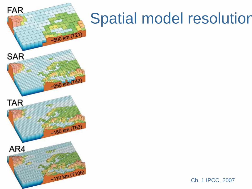
Spatial model resolution

Ch. 1 IPCC, 2007

Model runs and model experiments

Model runs:

• Control run (CTR): e.g. present-day climatology

• Experiment (EXP): - Transient runs (historical runs, RCP future runs, hindcast runs)

- Time slice runs (e.g. 2000 state runs)

- Perpetual runs (e.g. perpetual January runs)

Model experiment: a scientific question or model experiment should be

anwsered by implementing a model forcing to the model

- What is the effect of Arctic sea ice loss?

- What is the effect of greenhouse gas increase?

- What is the effect of ENSO on the atmosphere?

Model forcing – model response

• For a model experiment a forcing is prescribed: e.g. RCP8.5 scenario, volcanic and solar forcing, Arctic sea ice loss…

• Radiative forcing (IPCC Chapter 8): resulting radiative response to implemented model forcing

• Radiative (model) response -∆Rad= Rad(EXP)-Rad(CTR)

• Climate (model) response -e.g. ∆SAT=SAT(EXP)-SAT(CTR)

-e.g. ∆SST= SST(El Nino yrs)-SST(no ENSO yrs)

Main drivers of climate change

24

Chapter 1 IPCC (2013)

Pre-industrial perspective on radiative forcing factors (Section 5.2)

25

Radiative forcing factors

External forcing:

• Volcanic Forcing

• Solar Forcing

• Orbital Forcing

Greenhouse gases, aerosols, and dust:

• CO2, CH4, N2O, dust and aerosols

26

Last Millennium 1 ka- Reconstructed Volcanic forcing

based on ice core records

27

─Crowley and Unterman (2013) ─GRA: Gao, Robock and Ammann (2008 & 2012)

Stratospheric origin: ▀Greenland, ▄Antarctica

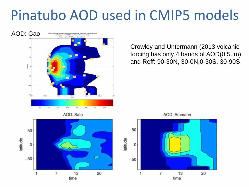
Pinatubo AOD used in CMIP5 models

28

Crowley and Untermann (2013 volcanic

forcing has only 4 bands of AOD(0.5um)

and Reff: 90-30N, 30-0N,0-30S, 30-90S

AOD: Gao

Continuous Flow Analysis of Ice Cores using CFA-BC-TE-GAS

Ultra Trace Chemistry Lab at DRI

By using black carbon measurements and many other parameters from new, real-time, high-resolution measurement techniques for annual layer dating, we could develop a history of sulfate deposition for Antarctica for the past 2,500 years.

3 cm 3 cm

slide provided by Michael Sigl

3) Volcanoes - ice cores

Volcanic ice-core synchronization

Sigl et al. 2014, Nature Clim. Change

Annual sulphur concentrations

With 12 records covering the past 1,500 years, we can reconstruct robust estimates of sulfate deposition on larger spatial scales.

531 UE ice cores vs 45Mt SO2 model r=0.48 b=4.1

Ice cores

o WAIS Divide chronology

3) Volcanoes - ice cores

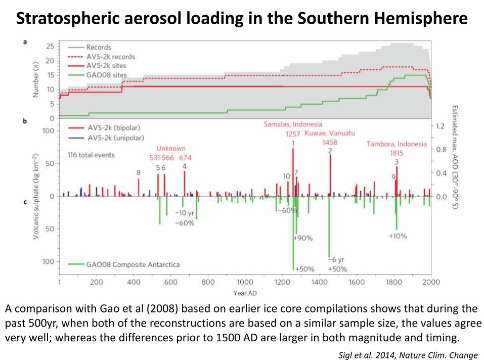
Stratospheric aerosol loading in the Southern Hemisphere

Sigl et al. 2014, Nature Clim. Change

A comparison with Gao et al (2008) based on earlier ice core compilations shows that during the past 500yr, when both of the reconstructions are based on a similar sample size, the values agree very well; whereas the differences prior to 1500 AD are larger in both magnitude and timing.

New bipolar ice core chronologies

1

Biomass Burning

Sea Salt

Marine Biogenic Emissions.

Dust

2

3 “StratiCounter”

10Be

14C

Revision of ice core chronologies in Greenland and Antarctica up to 10 years during 1st Millennium by: 1) using a fixed age marker in 775 CE, 2) constrained annual layer dating using multi-parameter aerosol records, 3) applying an objective algorithm.

Mekhaldi et al. in review

Ice cores

Tree rings

775 CE

slide provided by Michael Sigl

3) Volcanoes - ice cores

Post-volcanic cooling during the past 2,500 years

Sigl et al. 2015 Nature

1

0.5

0

-0.5

-1

-1.5

3) Volcanoes - ice cores

Last Millennium 1 ka

Reconstructed solar forcing

35 IPCC Chapter 5 (2013)

Solar activity proxy: sunspots and 10Be All reconstructions have been used for PIMP3/CMIP5 simulations expect Lean et al 1995b (LBB), which has been widely used before that.

Maunder Minimum 1645-1715

Temporal variations of the solar insolation

• The solar constant is not constant

• ~27-day rotation cycle of the sun

• ~11-year sunspot cycle

• Centennial scales

• Milankowich (1941): influence of the earth orbit parameter on the ice age cycles was confirmed by Hays et al. (1976).

37

The 11-year solar cycle

38

http://www.pmodwrc.ch/pmod.php?topic=tsi/composite/SolarConstant

Note new TSI value of ~1361 W/m2

taken from IPCC 2013 Chapter 8

ACRIM: Active Cavity Radiometer Irradiance Monitor TIM: Total Irradiance Monitor RMIB: Royal Meteorological Institute of Belgium PMOD: Physikalisch Meteorologisches Observatorium Davos

39

Kopp and Lean (2011)

TSI: Total Solar Irradiance

Historical reconstructions of TSI

TSI: Total Solar Irradiance 40

Ch

apte

r 8

IPC

C (

20

13

)

-Reconstructions are based on physical modeling of the evolution of solar surface magnetic flux... -All reconstructions rely on indirect proxies that inherently do not give consistent results. -Large discrepancies among the models.

43

Orbital Forcing

External climate factors Orbital parameters: 1. Eccentricity

Time in 1,000 yrs before today 0 200 400 600 800 1,000

0.06

0

100,000 years, 400,000 years

44

External climate factors Orbital parameters: 2. Obliquity of earth’s axis

Time in 1,000 yrs before today 0 200 400 600 800 1,000

0.06

0

24°

22°

Quelle: Ruddiman 2001

41,000 years

45

External climate factors Orbital parameters: 3. Precession

Time in 1,000 yrs before today 0 200 400 600 800 1,000

0.06

0

24°

22°

sin

-0.04

0.04

21,000 years

46

External climate factors Orbital parameters

Time in 1,000 years before today 0 200 400 600 800 1,000

0.06

0

Solar radiation in NH summer at 65°N

24°

22°

sin

-0.04

0.04

550

450

W/m2

47

Milankovitch theory orbital pacemaker for ice ages

W m-2

future time kyr BP past

65°N summer insolation

Eemian

interglacial

Last glacial

maximum … next ice age???

48

IPCC (2007) • “The Milankovitch, or ‘orbital’ theory of the ice ages is now well developed.

• Ice ages are generally triggered by minima in high-latitude NH summer insolation, enabling winter snowfall to persist through the year and therefore accumulate to build NH glacial ice sheets.

• Similarly, times with especially intense high-latitude NH summer insolation, determined by orbital changes, are thought to trigger rapid deglaciations, associated climate change and sea level rise.

• These orbital forcings determine the pacing of climatic changes, while the large responses appear to be determined by strong feedback processes that amplify the orbital forcing.

• Over multi-millennial time scales, orbital forcing also exerts a major influence on key climate systems such as the Earth’s major monsoons, global ocean circulation and the greenhouse gas content of the atmosphere.

• Available evidence indicates that the current warming will not be mitigated by a natural cooling trend towards glacial conditions.

• Understanding of the Earth’s response to orbital forcing indicates that the Earth would not naturally enter another ice age for at least 30,000 years. “

48

Past 3.5 Ma – Climate Changes

50 MPWP: Mid Pliocene Warm Period (3.3 to 3 Ma)

─ice cores │+/-2σ

Past 65 Ma - Atmospheric CO2

51 +/- 1σ uncertainty │+/- 2σ

Earth System Responses and Feedbacks (Section 5.3)

53

Past 800 ka

56

LIG: Last Interglacial H: Holocene

58

59

60

Reconstructions

64

----Reconstructions ▬ Instrumental period

NH

SH Global

NH surface temperature changes

66

MCA: Medieval Climate Anomaly LIA: Little Ice Age 20C: 20th Century

Models: -Strong solar variability sims -Weak solar variability sims ▬multi-model mean ─ multi-model 90% range

IPCC Chapter 5: Informations from paleoclimate archives

67

GEF4400 “The Earth System” – Autumn 2015 23.11.2015

Masson-Delmotte, V., et al., 2013: Information from Paleoclimate Archives. In: Climate Change 2013: The Physical Science Basis. Contribution of Working Group I to the Fifth Assessment Report of the Intergovernmental Panel on Climate Change. Cambridge University Press.

• Introduction (Section 5.1)

• Pre-industrial perspective on radiative forcing factors (Section 5.2)

• Earth System Responses and Feedbacks (Section 5.3)

• Executive summary (Ch. 5)

NH surface temperature changes

68

MCA: Medieval Climate Anomaly LIA: Little Ice Age 20C: 20th Century

Models: -Strong solar variability sims -Weak solar variability sims ▬multi-model mean ─ multi-model 90% range

Recap

Volcanic vs solar forcing and climate response

69

Cold-Warm Period: NH temp

MCA-LIA and 20C-LIA

70

MCA: Medieval Climate Anomaly LIA: Little Ice Age 20C: 20th Century

Executive Summary

86

Excecutive Summary -I

Greenhouse-Gas Variations and Past Climate Responses

• It is a fact that present-day (2011) concentrations of the atmospheric greenhouse gases (GHGs) carbon dioxide (CO2), methane (CH4) and nitrous oxide (N2O) exceed the range of concentrations recorded in ice cores during the past 800,000 years.

• With very high confidence, the current rates of CO2, CH4 and N2O rise in atmospheric concentrations and the associated radiative forcing are unprecedented with respect to the highest resolution ice core records of the last 22,000 years.

• There is high confidence that changes in atmospheric CO2 concentration play an important role in glacial–interglacial cycles. Although the primary driver of glacial–interglacial cycles lies in the seasonal and latitudinal distribution of incoming solar energy driven by changes in the geometry of the Earth’s orbit around the Sun (“orbital forcing”), reconstructions and simulations together show that the full magnitude of glacial–interglacial temperature and ice volume changes cannot be explained without accounting for changes in atmospheric CO2 content and the associated climate feedbacks.

87

With medium confidence, global mean surface temperature was significantly above pre-industrial levels during several past periods characterised by high atmospheric CO2 concentrations.

• During the mid-Pliocene (3.3 to 3.0 million years ago), atmospheric CO2 concentrations between 350 ppm and 450 ppm (medium confidence) occurred when global mean surface temperatures were 1.9°C to 3.6°C (medium confidence) higher than for pre-industrial climate.

• During the Early Eocene (52 to 48 million years ago), atmospheric CO2 concentrations exceeded ~1000 ppm (medium confidence) when global mean surface temperatures were 9°C to 14°C (medium confidence) higher than for pre-industrial conditions.

• New temperature reconstructions and simulations of the warmest millennia of the last interglacial period (129,000 to 116,000 years ago) show with medium confidence that global mean annual surface temperatures were never more than 2°C higher than pre-industrial.

88

Excecutive Summary - II

• There is high confidence that annual mean surface warming since the 20th century has reversed long-term cooling trends of the past 5000 years in mid-to-high latitudes of the Northern Hemisphere (NH). New continental- and hemispheric-scale annual surface temperature reconstructions reveal multi-millennial cooling trends throughout the past 5000 years. The last mid-to-high latitude cooling trend persisted until the 19th century, and can be attributed with high confidence to orbital forcing, according to climate model simulations. {5.5.1}

89

Excecutive Summary - III